15.4 Kronig Penney modelbingweb.binghamton.edu/.../15-4_Kronig_Penney_model.pdf · 2019-09-12 · 1...
17
1 Kronig Penney model Masatsugu Sei Suzuki Department of Physics, SUNY at Binghamton Binghamton, NY 13902-6000 (Date: March 23, 2018) _____________________________________________________________________________ Ralph Kronig was a German-American physicist (March 10, 1904 – November 16, 1995). He is noted for the discovery of particle spin and for his theory of x-ray absorption spectroscopy. His theories include the Kronig–Penney model, the Coster–Kronig transition and the Kramers–Kronig relation. http://en.wikipedia.org/wiki/Ralph_Kronig ______________________________________________________________________________ William George Penney, Baron Penney (24 June 1909– 3 March 1991), was an English mathematician and professor of mathematical physics at the Imperial College London as well as the rector of the imperial college. He is widely held responsible for his leading and integral role in the development of Britain's nuclear program, a clandestine programme started following the World war II and the success of Soviet nuclear program.
Transcript of 15.4 Kronig Penney modelbingweb.binghamton.edu/.../15-4_Kronig_Penney_model.pdf · 2019-09-12 · 1...

1
Kronig Penney model
Masatsugu Sei Suzuki
Department of Physics, SUNY at Binghamton
Binghamton, NY 13902-6000
(Date: March 23, 2018)
_____________________________________________________________________________
Ralph Kronig was a German-American physicist (March 10, 1904 – November 16, 1995). He is
noted for the discovery of particle spin and for his theory of x-ray absorption spectroscopy. His
theories include the Kronig–Penney model, the Coster–Kronig transition and the Kramers–Kronig
relation.
http://en.wikipedia.org/wiki/Ralph_Kronig
______________________________________________________________________________
William George Penney, Baron Penney (24 June 1909– 3 March 1991), was an English
mathematician and professor of mathematical physics at the Imperial College London as well as
the rector of the imperial college. He is widely held responsible for his leading and integral role in
the development of Britain's nuclear program, a clandestine programme started following the
World war II and the success of Soviet nuclear program.

2
http://en.wikipedia.org/wiki/William_Penney,_Baron_Penney
1. Kronig-Penney model
The essential features of the behavior of electrons in a periodic potential may be explained by
a relatively simple 1D model which was first discussed by Kronig and Penney. We assume that
the potential energy of an electron has the form of a periodic array of square wells.
Fig. Periodic potential in the Kronig-Penney model
We now consider a Schrödinger equation,
)()()()(2 2
22
xExxVxdx
d
m
ℏ,
where is the energy eigenvalue.
(i) V(x) = 0 for 0≤x≤a
iKxiKx BeAex )(1 , )(/)(1
iKxiKx BeAeiKdxxd ,
with mKE 2/22ℏ .
(ii) V(x) = U for -b≤x≤0
QxQx
DeCex)(2 , )(/)(2
QxQx DeCeQdxxd ,
with
-b 0 a a+bx
U
VHxL
3
mQEU 2/22ℏ .
The Bloch theorem can be applied to the wave function
)()( )( xebax baik ,
where k is the wave number. The constants A, B, C, and D are chosen so that and d/dx are
continuous at x = 0 and x = a.
(a) At x = 0,
DCBA ,
)()( DCQBAiK .
Thanks to the Bloch theorem, the boundary condition of the wave function at x b is related to
that at x a . In other words, we have only to know the knowledge of the wave function in a unit
cell (the period is a b ).
(b) At x = -b,
)()( )( bea baik , or )()( 2)(
1 bea baik ,
)(')(' )( bea baik , or )(')(' 2)(
1 bea baik ,
or
)()( QbQbbaikiKaiKa DeCeeBeAe ,
)()( )( QbQbbaikiKaiKa DeCeQeBeAeiK .
The above four equations for A, B, C, and D have a solution only if det[M]=0, where the matrix
M is given by

4
)()(
)()(
1111
baikQbbaikQbiKaiKa
baikQbbaikQbiKaiKa
QeQeiKeiKe
eeee
QQiKiKM .
The condition of det[M] = 0 leads to
)sinh()sin(2
)()cosh()cos()](cos[
22
QbKaKQ
KQQbKabak
.
where
mQEU 2/22ℏ , mKE 2/22
ℏ
or
)(2
222
QKm
U ℏ
.
The energy dispersion relation (E vs k) can be derived from this equation.
2. Numerical claculation
The essential features of the behavior of electrons in a periodic potential may be explained by
a relatively simple 1D model which was first discussed by Kronig and Penney. We assume that
the potential energy of an electron has the form of a periodic array of square wells.
Here we show only the result of the Kronig-Penny model:
((Mathematica))
Using the Mathematica, one can derive the fundamentak equation for the energy diagram in the
Kronig-Penney model.
5
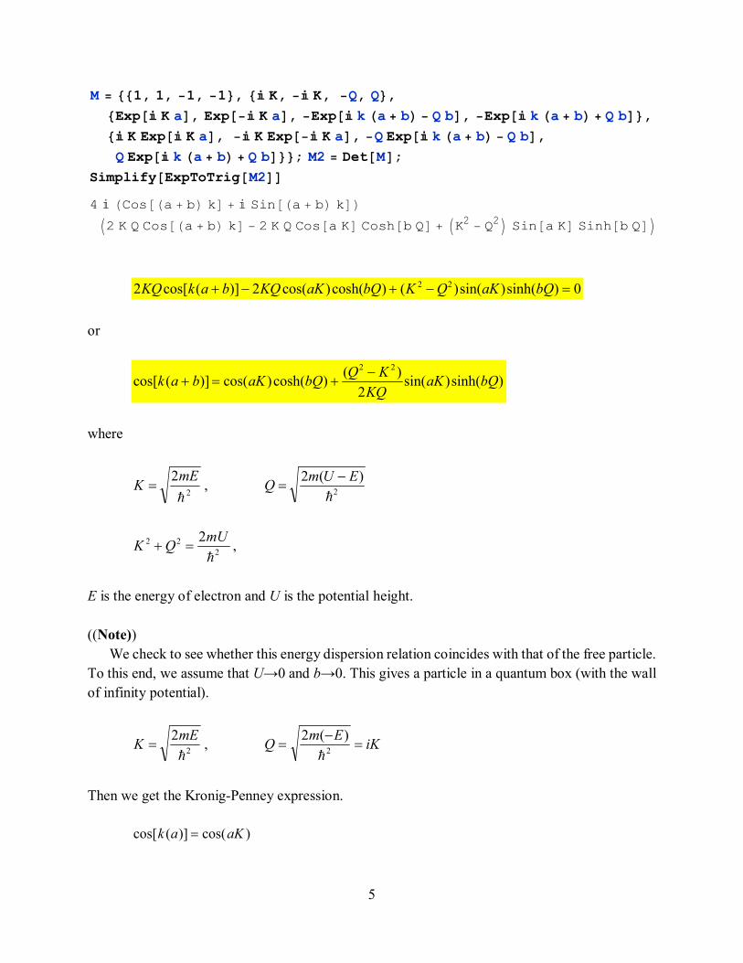
0)sinh()sin()()cosh()cos(2)](cos[2 22 bQaKQKbQaKKQbakKQ
or
)sinh()sin(2
)()cosh()cos()](cos[
22
bQaKKQ
KQbQaKbak
where
2
2
ℏ
mEK ,
2
)(2
ℏ
EUmQ
222 2
ℏ
mUQK ,
E is the energy of electron and U is the potential height.
((Note))
We check to see whether this energy dispersion relation coincides with that of the free particle.
To this end, we assume that U→0 and b→0. This gives a particle in a quantum box (with the wall
of infinity potential).
2
2
ℏ
mEK , iK
EmQ
2
)(2
ℏ
Then we get the Kronig-Penney expression.
)cos()](cos[ aKak
M = 881, 1, −1, −1<, 8� K, −� K, −Q, Q<,8Exp@� K aD, Exp@−� K aD, −Exp@� k Ha + bL − Q bD, −Exp@� k Ha + bL + Q bD<,8� K Exp@� K aD, −� K Exp@−� K aD, −Q Exp@� k Ha + bL − Q bD,Q Exp@� k Ha + bL + Q bD<<; M2 = Det@MD;
Simplify@ExpToTrig@M2DD4 � HCos@Ha + bL kD + � Sin@Ha + bL kDLI2 K Q Cos@Ha + bL kD − 2 K Q Cos@a KD Cosh@b QD + IK2 − Q2M Sin@a KD Sinh@b QDM
6
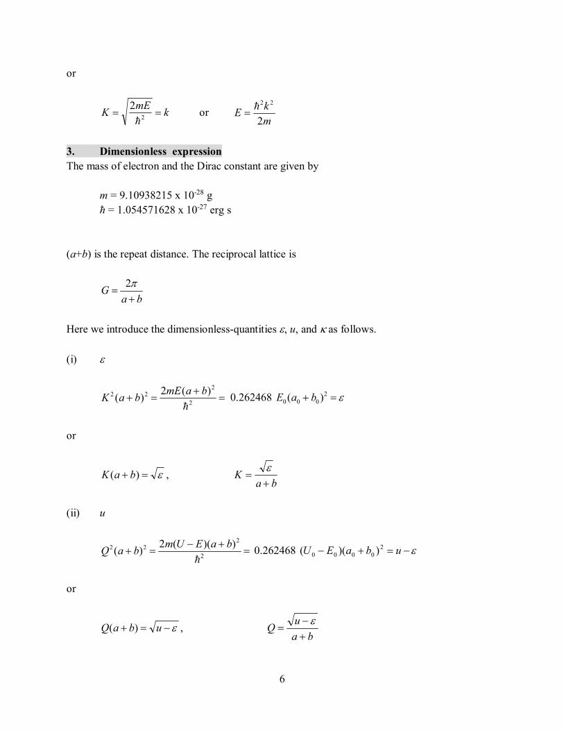
or
kmE
K 2
2
ℏ or
m
kE
2
22ℏ
3. Dimensionless expression
The mass of electron and the Dirac constant are given by
m = 9.10938215 x 10⁻²⁸ g
ħ = 1.054571628 x 10⁻²⁷ erg s
(a+b) is the repeat distance. The reciprocal lattice is
baG
2
Here we introduce the dimensionless-quantities , u, and as follows.
(i)
2
222 )(2
)(ℏ
bamEbaK 0.262468 2
000 )( baE
or
)( baK , ba
K
(ii) u
2
222 ))((2
)(ℏ
baEUmbaQ 0.262468 ubaEU 2
0000 ))((
or
ubaQ )( , ba
uQ

7
where
2
2)(2
ℏ
bamU 0.262468 ubaU 2
000 )(
(iii)
)()( 000 bakbak ba
k
((Note)) That a and b are in the units of Å, k is in the unit of Å-1, and E and U is the unit of eV.
In other words, a0, b0, k0, E0, and U0 are dimensionless.
0aa (Å), 0bb (Å), 0kk (Å-1),
0EE (eV), and 0UU (eV),
Then we get
1
1
ba
aaK
uu
ba
bbQ
1
)( bak
where
0
0
a
b
a
b .
Using the above parameters, the Kronig-Penney expression can be rewritten as
]1
sinh[)1
sin()2(
]1
cosh(]1
cos[2]cos[2
uu
uuu

8
or
]1
sinh[)1
sin(2
)2(]
1cosh(]
1cos[]cos[
u
u
uu
which means that the energy dispersion relation is dependent only on the values of and u.
4. Energy gap regions
Here we put the right hand side of the above equation as H(),
]1
sinh[)1
sin(2
)2(]
1cosh(]
1cos[)(
u
u
uuH
The left-hand side )cos( oscillates between -1 and 1. We make a plot of H() as a function of ,
where u is given as a parameter. The energy gap occurs in the energy range where |H()|>1.
Fig. The right hand side of the Kronig-Penney expression, H() as a function of , where
u = 100. = b/a = 0.1/3. The energy gap exists in the green zone where |H()|>1. = (9.87507 - 15.4575). = (39.5002 - 45.6691), = (88.8754 - 95.1686), and =
(158.0 - 164.288). The energy gap width () is the same
5. Energy dispersion relation (numerical calculation)

9
The energy dispersion relation ( vs k) can be determined the ContourPlot of the
Mathematica, where u and are given as parameters.
((Parameters))
u 0.262468 2
00aU
0
0
a
b
a
b
(i) units of horizontal and vertical axes for the energy dispersion relation
00
0ba
k
(given in the unit of Å-1)
2
0
0262468.0 a
E
(given in the unit of eV)
Note that k0 and E0 are dimension-less.
(ii) Brillouin zone boundary of the first Brillouin zone
B.
(iii) Empty lattice approximation: Free electron model
2)2( Bn
where n = 0, ±1, ±2, ......
((Example))
b/a = 0.1/3. u = 100.

10
Fig. Kronig-Penney energy band in the extended zone scheme. b/a = 0.1/3. u = 100.
When a0 = 5 (Å), E0 = /6.5617 (eV). It means that E0 = 15.24 eV for = 100.

11
Fig. Kronig-Penney energy band in the reduced zone scheme. b/a = 0.1/3. u = 100.
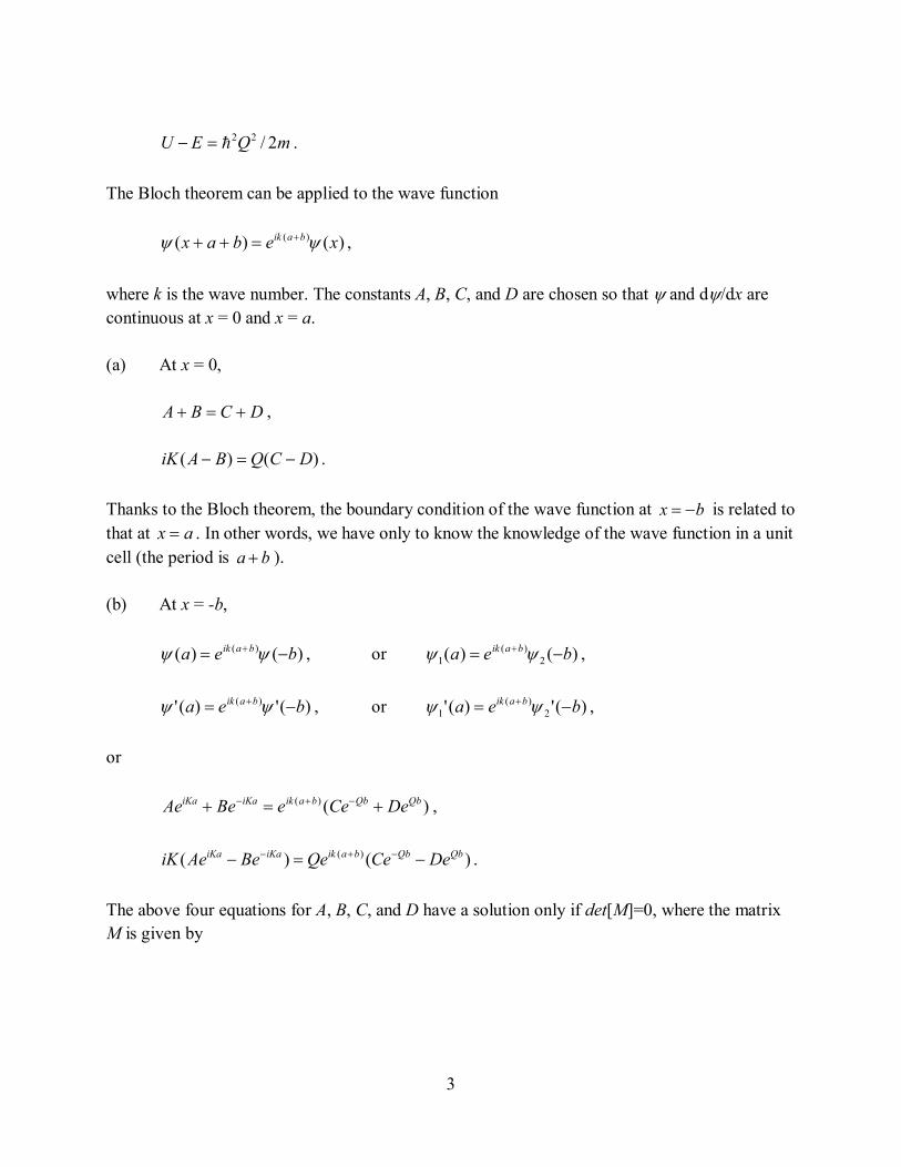
5. Dirac delta function
The Result of Kronig-Penney can be simplified if we represent the potential by the periodic
delta function.
We start with the equation given by
)sinh()sin(2
)()cosh()cos()](cos[
22
bQaKKQ
KQbQaKbak
We assume the limit b = 0 and U = ∞ such a way that
1Ub .

12
In this limit,
KQ and Qb<<1.
We note that
1)cosh( bQ
Ka
Pab
Ka
QbQ
KQ
QbQ
KQ
KQ
22
)sinh(2
)( 2222
Fig. Dirac-comb type potential energy with the separation distance a.
Then we have
aK
aKPaKka
)sin()cos()cos(
with
2
2abQP
where P remains constant as a fixed parameter.
x
VHxL
a 2a 3a-a-2a-3a 0
13
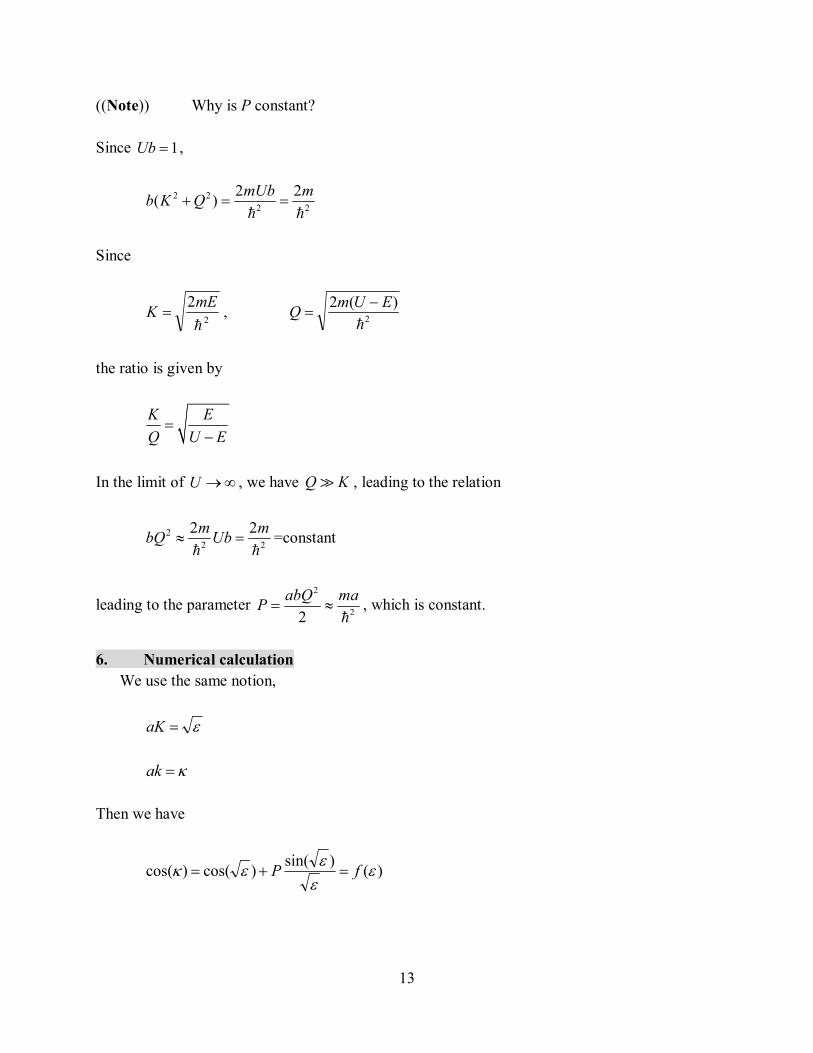
((Note)) Why is P constant?
Since 1Ub ,
2 2
2 2
2 2( )
mUb mb K Q
ℏ ℏ
Since
2
2
ℏ
mEK ,
2
)(2
ℏ
EUmQ
the ratio is given by
K E
Q U E
In the limit of U , we have Q K≫ , leading to the relation
2
2 2
2 2m mbQ Ub
ℏ ℏ=constant
leading to the parameter 2
22
abQ maP
ℏ, which is constant.
6. Numerical calculation
We use the same notion,
aK
ak
Then we have
)()sin(
)cos()cos(
fP

14
We make a plot of f() as a function of . P is a parameter. When )sin( =0 ( , 2, 3),
the value of f() is independent of P.
Fig. Plot of f() as a function of , where P is changed as a parameter. P = /2 (red),
(orange), 3/2 (green), 2 (dark green), and 5/2 (blue). Allowed state in the region
where |f()|<1 (the purple zone). The forbidden states in the region where |f()|>1.
The energy gap increases with increasing P.
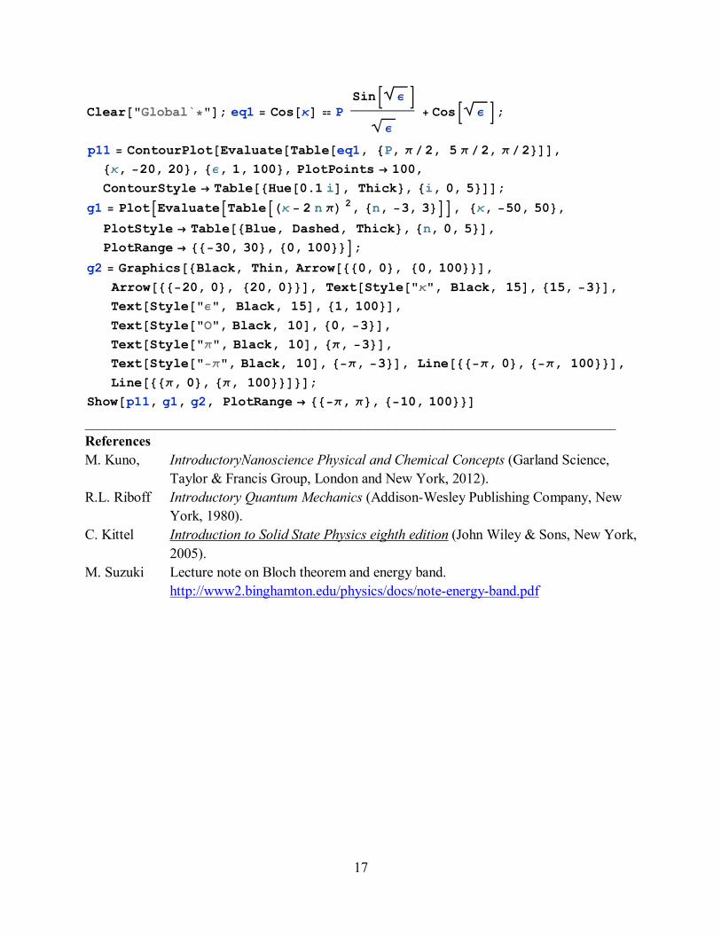
Using the ContourPlot of the Mathematica, we can draw the vs diagram for each P.

15
Fig. Energy band in the expended Brillouin zone. P = /2 (red), , 3 /2, 2, 5 /2 (green).
The dashed lines (blue) are described by (- 2n)2.
k
e
O p-p
-20 -10 0 10 20
0
20
40
60
80
100

16
Fig. Energy band in the reduced Brillouin zone. 8. Summary
The following interesting conclusions may be derived from the above figures. (a) The energy spectrum of the electrons consists of a number of allowed energy bands separated
by energy gaps. (b) The discontinuities in the energy spectrum, occur for the zone boundaries.
APPENDIX
Mathematica program for the Kronig-Penney model with Dirac-comb type potential
e
O p-p
-3 -2 -1 0 1 2 3
0
20
40
60
80
100
17
___________________________________________________________________________ References
M. Kuno, IntroductoryNanoscience Physical and Chemical Concepts (Garland Science, Taylor & Francis Group, London and New York, 2012).
R.L. Riboff Introductory Quantum Mechanics (Addison-Wesley Publishing Company, New York, 1980).
C. Kittel Introduction to Solid State Physics eighth edition (John Wiley & Sons, New York,
2005). M. Suzuki Lecture note on Bloch theorem and energy band.
http://www2.binghamton.edu/physics/docs/note-energy-band.pdf
Clear@"Global`∗"D; eq1 = Cos@κD � P
SinB ε F
ε
+ CosB ε F;
p11 = ContourPlot@Evaluate@Table@eq1, 8P, π ê2, 5 π ê2, π ê2<DD,8κ, −20, 20<, 8ε, 1, 100<, PlotPoints → 100,
ContourStyle → Table@[email protected] iD, Thick<, 8i, 0, 5<DD;g1 = PlotAEvaluateATableAHκ − 2 n πL 2, 8n, −3, 3<EE, 8κ, −50, 50<,
PlotStyle → Table@8Blue, Dashed, Thick<, 8n, 0, 5<D,PlotRange → 88−30, 30<, 80, 100<<E;
g2 = Graphics@8Black, Thin, Arrow@880, 0<, 80, 100<<D,Arrow@88−20, 0<, 820, 0<<D, Text@Style@"κ", Black, 15D, 815, −3<D,Text@Style@"ε", Black, 15D, 81, 100<D,Text@Style@"O", Black, 10D, 80, −3<D,Text@Style@"π", Black, 10D, 8π, −3<D,Text@Style@"−π", Black, 10D, 8−π, −3<D, Line@88−π, 0<, 8−π, 100<<D,Line@88π, 0<, 8π, 100<<D<D;
Show@p11, g1, g2, PlotRange → 88−π, π<, 8−10, 100<<D