IWAA08, G. Moss

113.02.2008

WarsawUniversity

LiCAS

Linear Collider Alignment & Survey

The LiCAS LSM SystemFirst measurements from the Laser Straightness Monitor

of the LiCAS Rapid Tunnel Reference Surveyor.

13.02.2008

IWAA08, G. Moss

2

Contents LiCAS Overview Straightness Monitor

Basics Produced system Beam Fitting Stability The Ray tracer Reconstruction Calibration Autocalibration Conclusions

13.02.2008

IWAA08, G. Moss

3

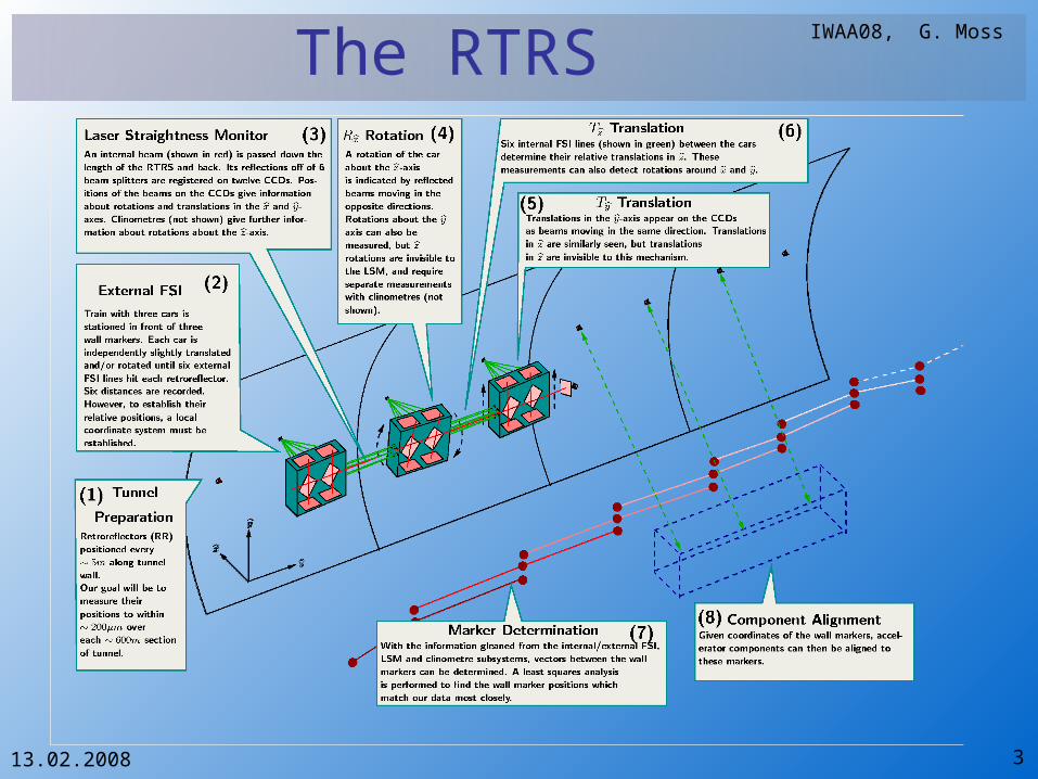
The RTRS

13.02.2008

IWAA08, G. Moss

4

Sensitivity of Internal Components

Component

TrX TrY TrZ RotX RotY

RotZ

LSM √ √ √ √

FSI ± ± √ ± ±

Inclinometer

√(not used)

√

13.02.2008

IWAA08, G. Moss

5

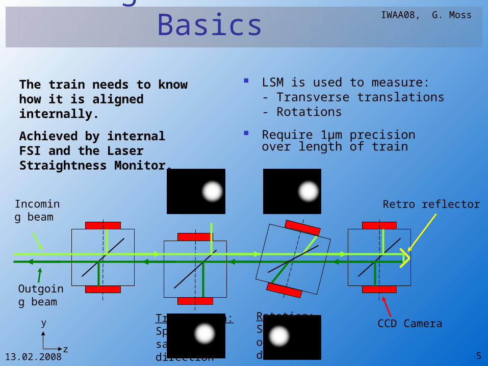
Straightness Monitor Basics

LSM is used to measure:- Transverse translations- Rotations

Require 1µm precision over length of train

z

y Translation:Spots move same direction

Rotation:Spots move opposite directions

CCD Camera

Retro reflectorIncoming beam

Outgoing beam

The train needs to know how it is aligned internally.

Achieved by internal FSI and the Laser Straightness Monitor.

13.02.2008

IWAA08, G. Moss

6

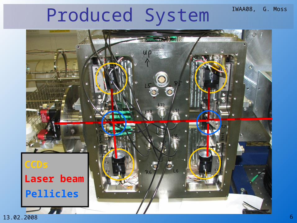
Produced System

CCDsLaser beamPellicles

13.02.2008

IWAA08, G. Moss

7

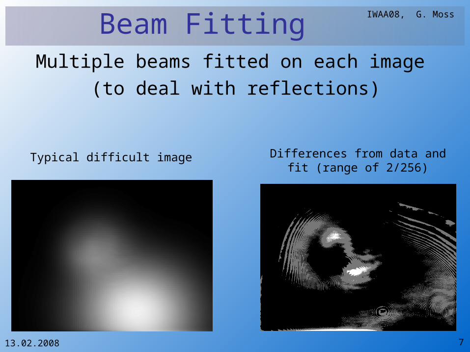
Beam FittingMultiple beams fitted on each image

(to deal with reflections)

Typical difficult image Differences from data and fit (range of 2/256)

13.02.2008

IWAA08, G. Moss

8

Beam Fitting Real life beams fitted over 40 hours to: 1.28μm horizontally 0.54μm vertically Difference not understood – possibly

beam jitter

13.02.2008

IWAA08, G. Moss

9

Stability Large amount of data taken with no

planned movement

2 x 10 images every 10 minutes Data taken for 4 days

13.02.2008

IWAA08, G. Moss

10

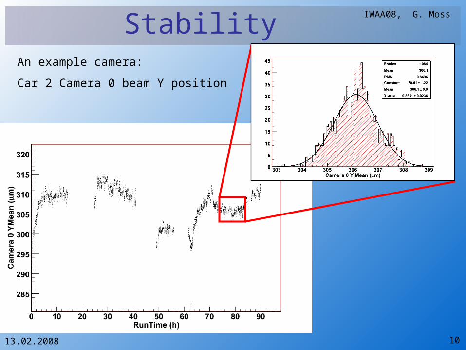
StabilityAn example camera:

Car 2 Camera 0 beam Y position

13.02.2008

IWAA08, G. Moss

11

Stability

Laser power increased here

0.78μm Standard deviation

0.55μm Standard deviation per camera. (Same as earlier)

Camera 2Camera 0 + Camera 2Camera 0 + Camera 2 added

13.02.2008

IWAA08, G. Moss

12

Stability

Launch/car1 are unstable to the order of 4 micro-radians over 4 days.

Motion of ~35μm on car3 (9.2m away)

Motion of ~15μm on car2 (4.7m away)

Motion of ~1μm on car1 (0.2m away & attached)

13.02.2008

IWAA08, G. Moss

13

The LSM

CCDsLaser beamPellicles

13.02.2008

IWAA08, G. Moss

14

Ray Tracer•Ray tracer used to calculate spot positions

•Highly flexible

•Agrees with completely independent Simulgeo simulation

13.02.2008

IWAA08, G. Moss

15

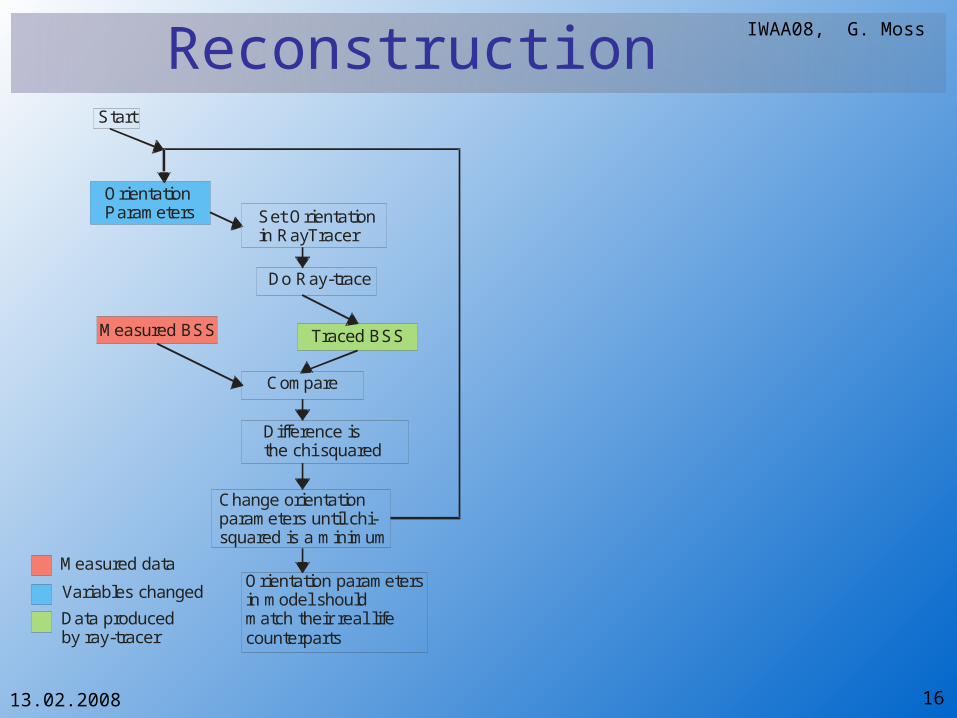
ReconstructionRay tracer is used as a part of a fit function for

the Minuit fitting package

Position & orientation of each LSM unit used as the fit parameters

CCD spots fitted by Chi-squared Minimisation Precise to ~0.5xSpot uncertainty for translations

~0.3 microns Precise to ~5xSpot uncertainty for rotations

~3 microradians Easy to take many images, average, then fit or fit

then average.

13.02.2008

IWAA08, G. Moss

16

Reconstruction

Orientation Parameters

Do Ray-trace

Traced BSSMeasured BSS

Compare

Difference isthe chi squared

Set Orientationin RayTracer

Change orientationparameters until chi-squared is a minimum

Orientation parametersin model should match their real life counterparts

Measured data

Variables changed

Data produced by ray-tracer

Start

13.02.2008

IWAA08, G. Moss

17

Internal Geometry

Model used needs correct geometry Camera positions & orientations Pellicle positions & orientations

These are the calibration constants Measured to 5-10 microns with CMM Need to know some better

13.02.2008

IWAA08, G. Moss

18

Constant ImportanceFractional Effect of Calibration Constant Errors

on X Reconstruction

-1.92E -05

-2.44E -05

-8.62E -05

-3.46E -05

0.0137672

0.0242108

0.00922344

0.00674144

-0.0137672

0.00236188

-0.00638842

0.00330743

0.00901177

-0.0179043

-0.00471597

-0.00426068

0.247563

-0.00162873

-0.00285011

-0.00681383

0.000784621

0.00940945

0.25524

-0.000568239

0.00261698

0.00384359

-4.70E -06

0.249913

0.00137205

0.00175043

0.0206908

-0.00990215

0.00122841

0.248757

-0.00119316

0.00416492

0.00387589

0.00299668

-0.0164883

0.00380746

-0.30 -0.20 -0.10 0.00 0.10 0.20 0.30

Ca

lib

rati

on

Co

ns

tan

t

Fractional Effect

Fractional Effect of Calibration Constant Errors on Y Reconstruction

0.000232296

7.54E -05

-3.61E -05

1.16E -04

-0.0393707

0.542851

0.510581

-0.0186342

0.0354872

0.0321918

0.017355

0.51903

0.519738

0.0298428

0.00218116

-0.016493

-0.0112241

-0.0227298

-0.237067

-0.0186867

0.0091897

0.00853597

0.00627214

0.00698782

-0.233642

-0.0124712

0.0349322

0.0315577

-0.032755

-0.237208

-0.000936036

-0.0289897

0.00751996

0.0611489

-0.00809303

-0.245866

0.0279941

-0.0152319

0.0284279

0.0282809

-0.60 -0.40 -0.20 0.00 0.20 0.40 0.60

Ca

lib

rati

on

Co

ns

tan

t

Fractional Effect

Fractional Effect of Calibration Constant Errors on X Rotation Reconstruction

0.00148791

0.00170907

0.000508503

0.000896225

-0.142667

2.40725

2.52964

0.524659

-0.0344198

0.0575502

-0.173775

-2.44857

-2.43335

0.393972

0.0327378

-0.0911257

0.0690915

-0.0982474

-0.0549693

-0.36683

-0.0802124

0.0984274

0.102507

-0.0780714

-2.63525

0.162835

-0.00473015

0.101802

0.0347473

2.47235

0.265889

0.174575

-0.150524

-0.0888212

-0.101556

0.187312

0.0177157

-0.00983479

-0.0433176

0.0211725

-3.00 -2.00 -1.00 0.00 1.00 2.00 3.00

Ca

lib

rati

on

Co

ns

tan

t

Fractional Effect

Fractional Effect of Calibration Constant Errors on Y Rotation Reconstruction

-0.000338973

-0.000396597

-0.000436897

-1.22E -05

-0.069971

0.0331497

0.0226464

0.0808236

0.18408

-0.249641

-0.120422

0.0440838

0.0320906

0.0664203

0.255743

-0.233498

0.0151639

0.0233963

-0.0565556

0.0145145

-0.0210639

-0.0481545

-2.43072

0.00614492

0.0153731

0.0758632

-0.162739

2.42701

-0.103565

0.00711689

-0.0102406

-0.0353695

-0.055106

-0.0834477

0.0763176

0.0233914

0.0407057

-0.0744809

-0.0576272

-0.027149

-3.00 -2.00 -1.00 0.00 1.00 2.00 3.00

Ca

lib

rati

on

Co

ns

tan

t

Fractional Effect

Important Constants

CCD Y positions

CCD Z positions

Pellicle Y positions

Pellicle Z positions

1 micron error in parameter gives 0.25 – 0.5 micron / 2.5 – 5.0 microradian error in reconstructed parameter

13.02.2008

IWAA08, G. Moss

19

Classical Calibration

•This method compares spot positions generated using a set of calibration constants, to the measured values (knowing the correct orientation).

•Many orientations are used

•It changes the calibration constants until the difference between the measured spots is minimised.

•Complements linear algebra method (see presentation by A. Reichold.)

True Orientation (measured by laser tracker)

Setup RayTracer

Calibration Constants

Do Ray-trace

Traced BSSMeasured BSS(taken by cameras)

Compare

Add difference tototal chi squared

Set Correct Orientation

For n Orientations

Change calibration constants until chi-squared is a minimum

Calibration constantsin model should match their real life counterparts

Measured data

Variables changed

Data produced by ray-tracer

Start

13.02.2008

IWAA08, G. Moss

20

Classical Calibration Simulation run with typical values:

1μm camera resolution 3μm/10μradian observation error 80 orientations used 1mm component uncertainty

Important constants found to < 1 μm Other constants found to <100 μm (not

that useful)

13.02.2008

IWAA08, G. Moss

21

Classical Calibration Now USE the fitted constants Reconstruct many times and compare to the truth Mean residual gives systematic error of that system Standard Deviation is dominated by camera resolution – gives

statistical error of that system

Offset: 0.18μm

Offset: 0.69μ radians

Offset: -0.36μm

Offset: 2.80μ radians

Example run shown on right.

However – this is only one example. Would like to know what to expect in general.

13.02.2008

IWAA08, G. Moss

22

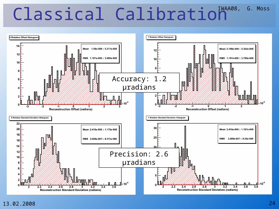
Classical Calibration Run simulation many times (with 0.1

mm component uncertainty) Collect the mean and standard

deviation values of the histograms produced

Create a histogram of these values For the mean histogram the standard

deviation gives the accuracy For the standard deviation histogram

the mean gives the precision

13.02.2008

IWAA08, G. Moss

23

Classical Calibration

Accuracy: 0.3 μm

Precision: 0.5 μm

13.02.2008

IWAA08, G. Moss

24

Classical Calibration

Precision: 2.6 μradians

Accuracy: 1.2 μradians

13.02.2008

IWAA08, G. Moss

25

Auto-Calibration

E = External unknowns (reconstructed variables) I = Internal unknowns (calibration constants) M = Measurements

M = F(E,I) Eg for a single LSM reading

8 measurements (CCD spot positions) 4 external unknowns 18 internal constant unknowns

(this is underconstrained) For 10 readings

80 measurements 40 external unknowns 18 internal constant unknowns

(This is overconstrained by 22 DoF)

We use the large overconstraint found with many readings to determine the calibration constants.

Complements both classical calibration methods Can be used with much more data and can show how constants change.

13.02.2008

IWAA08, G. Moss

26

Auto-Calibration

This method incorporates the calibration constants as part of the fitting process

Many runs are fitted en-masse and the individual chi-squareds summed

The constants that give the lowest total chi-squared are chosen.

S etup R ayTracer

C a lib ra tion C ons tan ts

M easured B S S(taken by cam eras)

R econstruc t

A dd to to ta l ch i squa red

F or n se ts o f beam spots

C hange ca lib ra tion cons tan ts un til to ta l ch i-squa red is a m in im um

C a lib ra tion constantsin m ode l shou ld m atch the ir rea l life coun terpa rts

M easured da ta

Variab les changedD a ta p roducedby reconstructo r

S ta rt

R econstruc tedO rien ta tion

D isca rdedC h i-S quared from fit

13.02.2008

IWAA08, G. Moss

27

Auto-Calibration Simulations have been performed using

typical uncertainties 40 runs 1μm camera resolution 0.1mm constant uncertainty

Find most important constants to <0.3μm (after corrections)

Problems (as expected) with scaling & offsets

Still a useful addition to calibration

13.02.2008

IWAA08, G. Moss

28

Conclusions Working LSM system Beam fitting now mature Stability under investigation Ray tracer well developed Reconstruction effective Calibration predicted to work well Autocalibration predicted to

compliment well