Mech 311 Lecture 1 1

Lecture 1

Introduction

Credits: 3.75 Session: Fall

Time: _ _ W _ F 13:15 - 14:30

MECH 311 Manufacturing Processes

–Section X

Instructor: Sivakumar Narayanswamy

Objective of the course

To provide the basic understanding of

• Measurements,

• Tolerancing and

• Design and understanding of different manufacturing methods ( Conventional and non-conventional).

• Feel for manufacturing:

– What machine at what situation?

– What is possible by existing manufacturing methods?

– Cost effective routes!

– Feel for numbers!

How to Ensure?

what we produce is what we want.

Inspection

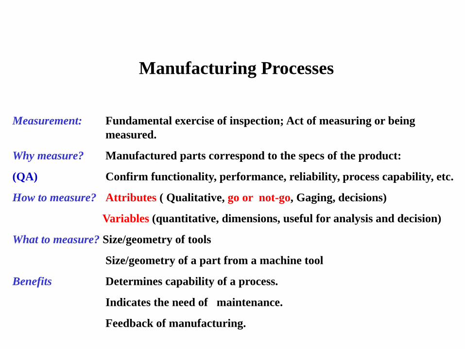
Manufacturing Processes

Measurement: Fundamental exercise of inspection; Act of measuring or being

measured.

Why measure? Manufactured parts correspond to the specs of the product:

(QA) Confirm functionality, performance, reliability, process capability, etc.

How to measure? Attributes ( Qualitative, go or not-go, Gaging, decisions)

Variables (quantitative, dimensions, useful for analysis and decision)

What to measure? Size/geometry of tools

Size/geometry of a part from a machine tool

Benefits Determines capability of a process.

Indicates the need of maintenance.

Feedback of manufacturing.

Attribute Vs Dimensional

• Qualitative

• Fast and economical

• Pass or fail

• Mostly for standard and

less severe applications

(Automobile)

• Useful after process

development

• Large production volume

• Quantitative

• Slow and expensive

• Exact dimension is needed

• Useful for highly reliable

applications (Aircrafts)

• Needed for development

• Small production volume

Standard Measurements:

Issues Units are different => Conversion scales

Linear Standards

Metric Systems ANSI System

1in ~ 41,929.399 wavelengths related to human body

sizes Of orange-red light Kr86

Standard set of rectangular gage blocks with ±0.000050-in.

Wrung-together gage blocks

in a special holder, used with

a dial gage to form an

accurate comparator.

Screw gage blocks wrung together to build

up a desired dimension.

Length Standards: Gage blocks or slip gages (Alloy

steel with Rc65)

Standard gages of meter – exist in any workshop ( standard blocks); need to calibrate

every specific period ( various precision).

Calibrated at 20°C

Accuracy Vs. Precision

Accuracy: ability to reach the aimed size

Precision: repeatability of accuracy

(Left):Accuracy versus precision. Dots in targets represent location of shots.

Cross (X) represents the location of the average position of all shots.

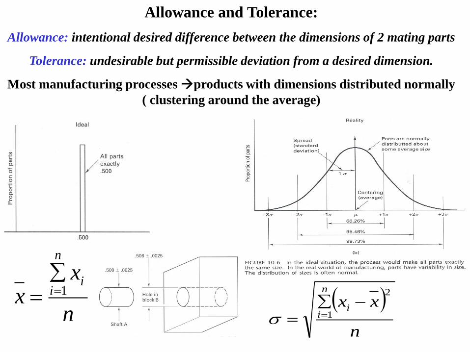
Allowance and Tolerance:

Allowance: intentional desired difference between the dimensions of 2 mating parts

Tolerance: undesirable but permissible deviation from a desired dimension.

Most manufacturing processes products with dimensions distributed normally

( clustering around the average)

n

xx

i

n

i 1

n

xxi

n

i

2

1

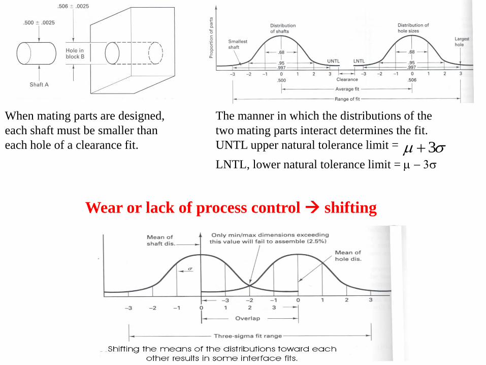
The manner in which the distributions of the

two mating parts interact determines the fit.

UNTL upper natural tolerance limit = 3LNTL, lower natural tolerance limit = 3

When mating parts are designed,

each shaft must be smaller than

each hole of a clearance fit.

Wear or lack of process control shifting

Clearance?

Range of Fit?

MMC?

LMC?

Bilateral?

Unilateral?

Limits

How to Specify Tolerances?

ANSI – 8 classes of fits

•Class 1. Loose fit: large allowance. Accuracy is not essential.

•Class 2. Free fit: Liberal allowance. For running fits where speeds are above 600 rpm and

pressures are 600 psi ( 4.1 MPa) or above

•Class 3. Medium Fit: Medium allowance. For running fits below 600 rpm and pressure below

600 psi ( 4.1 MPa) and for sliding fits.

•Class 4. Snug Fit: Zero allowance. No movement under load is intended, and no shaking is

wanted. This is the tightest fit that can be assembled by hand

•Class 5. Wringing fit: zero to negative allowance. Assemblies are selective and not

interchangeable.

•Class 6. Tight fit: slight negative allowance. An interface fit for parts that must not come

apart in service and are not to be disassembled or are to be disassembled only seldom. Light

pressure is required for assembly. Not to be used to with stand other than very light loads.

•Class 7. Medium force fit: an interference fit requiring considerable pressure to assemble;

ordinarily assembled by heating the external member or cooling the internal member to provide

expansion or shrinkage. Used for fastening wheels, crank disks, and the like to shafting. The

tightest fit that should be used on cast iron external members.

•Class8. Heavy force and Shrink fits: considerable negative allowance. Used for permanentshrink on steel members.

ISO System of Limits and Fits• Clearance fits

• Transition fits/ Location fits/ Assembly fits

• Interference fits

Shaft-basis and hole-basis system for specifying fits in the ISO system

What is Hole based or Shaft based system?

WHY?

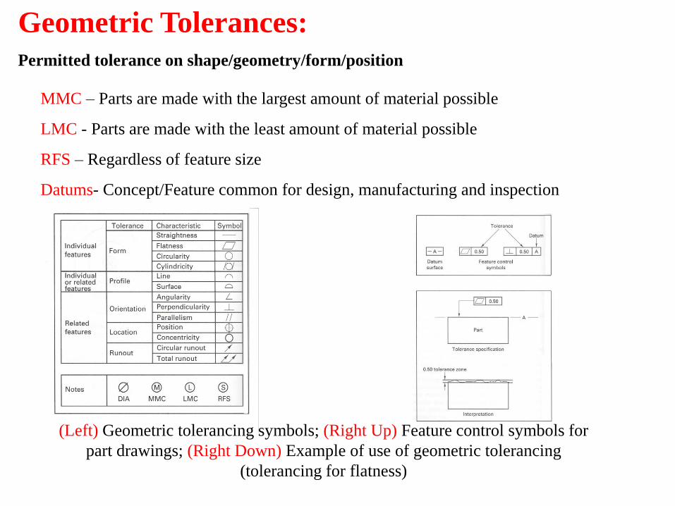
Geometric Tolerances:Permitted tolerance on shape/geometry/form/position

(Left) Geometric tolerancing symbols; (Right Up) Feature control symbols for

part drawings; (Right Down) Example of use of geometric tolerancing

(tolerancing for flatness)

MMC – Parts are made with the largest amount of material possible

LMC - Parts are made with the least amount of material possible

RFS – Regardless of feature size

Datums- Concept/Feature common for design, manufacturing and inspection

Inspection methods for measurement

Metrology: measurement laboratory selected according to certain criteria:

• Gage capability ( rule of 10)

Measuring device has to be 10times more precise than the tolerance measured:

Eg. +/-0.001 +/-0.0001 +/-0.00001

•Linearity

Linear working range (Input Vs Output)

•Repeat accuracy

Repeatability of the measurement

•Stability

Retaining calibration over time, no-drift

•Magnification

Amplification of the output portion of the device, bigger dials.

•Resolution

Sensitivity; smallest input value that can be detected or measured

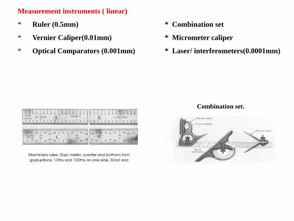
Measurement instruments ( linear)

* Ruler (0.5mm) * Combination set

* Vernier Caliper(0.01mm) * Micrometer caliper

* Optical Comparators (0.001mm) * Laser/ interferometers(0.0001mm)

Combination set.

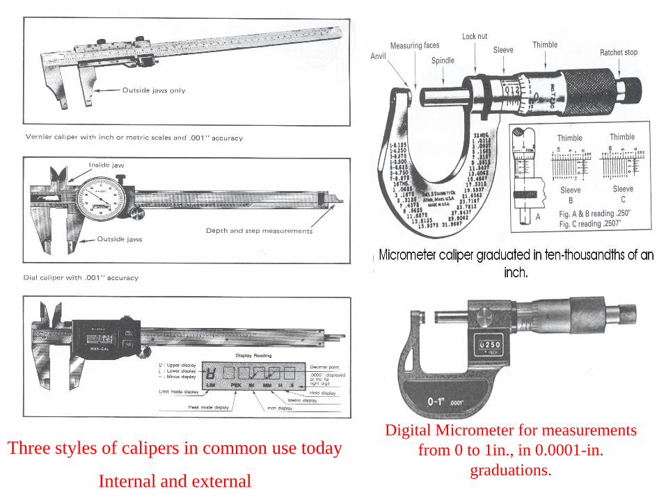
Three styles of calipers in common use today

Internal and external

Digital Micrometer for measurements

from 0 to 1in., in 0.0001-in.

graduations.

Vision Systems of measurement

Optical Comparator,

measuring the contour on a

workpiece. Digital indicators

with in/.mm conversions add

to the utility of optical

comparators.

Coordinate measuring

machine with inset showing

probe and a part being

measured.

Coordinate Measuring Machines

(CMM)

Interference bands can be used to measure the size of objects to great accuracy

a a)(bottom left) Calibrating the X-axis linear table displacement of a vertical

spindle milling machine; b) ( top right) Schematic of optical setup ; c) ( bottom

right) Schematic of components of a two frequency laser interferometer.Resolution ~ 10nm

The principle of the optical flat

Angle Measurement

• Sine Bar: 1sec of arc

Setup to measure an angle on a part using a

sine bar. The dial indicator is used to

determine when the part surface X is parallel

to the surface plate

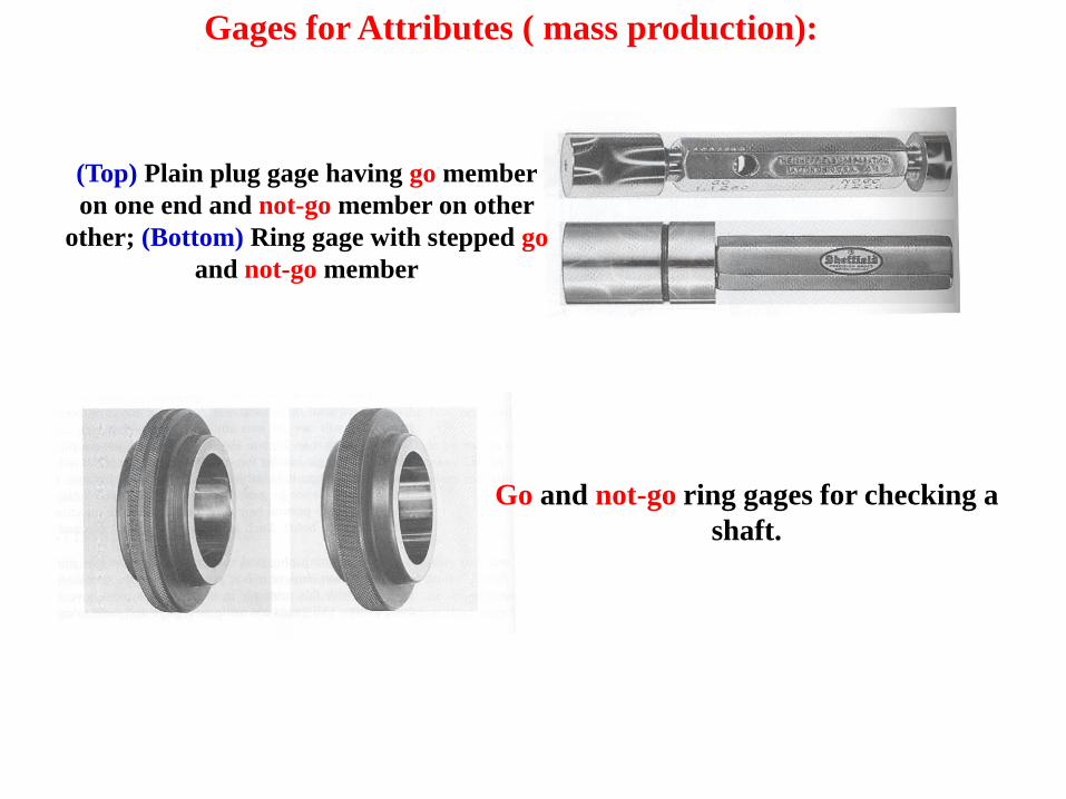
(Top) Plain plug gage having go member

on one end and not-go member on other

other; (Bottom) Ring gage with stepped go

and not-go member

Go and not-go ring gages for checking a

shaft.

Gages for Attributes ( mass production):

Ring Gage

GO

Ring gage

No GO

100+/- 0.1

Shaft

100.1 99.9

Plug gage

GO

Plug gage

NO GO

100+/- 0.1

Hole

99.9 100.1

Top) Microtopographer, a stylus profile device used to measure

and depict surface roughness and character (surface profile);

Bottom) Typical surface-roughness profiles.

Schematic of surface profile as produced

by stylus device showing some typical y

values with respect to the center line.

Schematic of stylus profile device for measuring

surface roughness and surface profile with two

readout devices shown: a meter for AA or rms

values and a strip-chart recorder for surface

profile.

Surface Roughness Measurement Instruments:

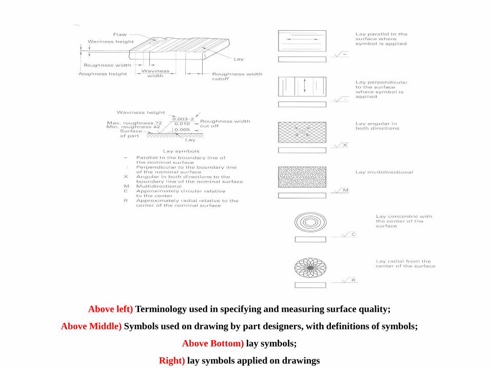
Above left) Terminology used in specifying and measuring surface quality;

Above Middle) Symbols used on drawing by part designers, with definitions of symbols;

Above Bottom) lay symbols;

Right) lay symbols applied on drawings

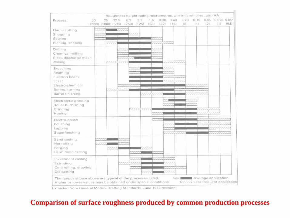
Comparison of surface roughness produced by common production processes

• Tolerance, Roughness and process are

interconnected.

• Selection of one determines the other.

• Eg: +/-0.5mm, Ra=0.1um no sense

+/- 0.01mm, Ra=25um no sense

Nondestructive Inspection and Testing:Ex: Strength of a part

Destructive Non-Destructive

Quantitative results Qualitative results

Do not require

interpretation

Skilled interpretation of

results

Restricted for costly

measurements

Low material cost

High cost equipment Low cost equipment

Consistent results More subjective results

Visual Inspection the first inspection method

Liquid (Dye)-penetrant inspection (LPI or DPI)

To be done prior to surface finishing or surface modifying operations,

like, shot peeing, polishing, etc.

Magnetic particle inspection (MPI)

•Only for Ferromagnetic Materials (Fe, Ni, Co

Alloys)

•Surface and sub surface flaws

•Orientation dependent, Perpendicular to the lines

•Parallel defects will not be detected

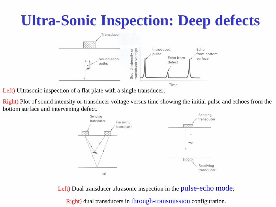
Left) Ultrasonic inspection of a flat plate with a single transducer;

Right) Plot of sound intensity or transducer voltage versus time showing the initial pulse and echoes from the

bottom surface and intervening defect.

Left) Dual transducer ultrasonic inspection in the pulse-echo mode;

Right) dual transducers in through-transmission configuration.

Ultra-Sonic Inspection: Deep defects

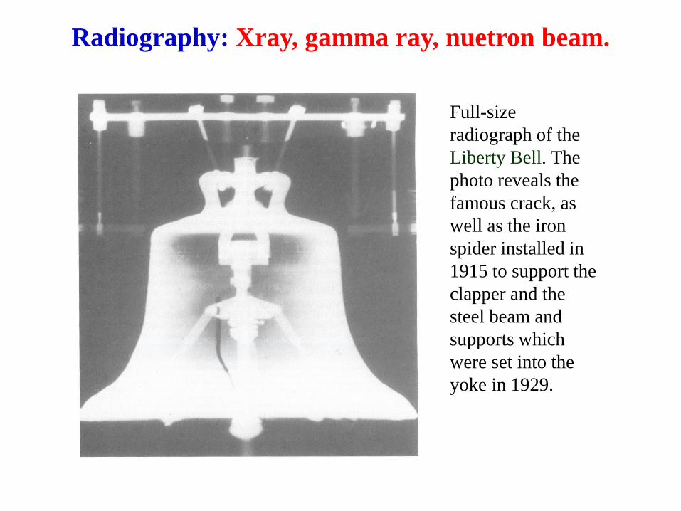
Radiography: Xray, gamma ray, nuetron beam.

Full-size

radiograph of the

Liberty Bell. The

photo reveals the

famous crack, as

well as the iron

spider installed in

1915 to support the

clapper and the

steel beam and

supports which

were set into the

yoke in 1929.

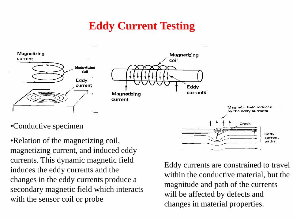
•Conductive specimen

•Relation of the magnetizing coil,

magnetizing current, and induced eddy

currents. This dynamic magnetic field

induces the eddy currents and the

changes in the eddy currents produce a

secondary magnetic field which interacts

with the sensor coil or probe

Eddy currents are constrained to travel

within the conductive material, but the

magnitude and path of the currents

will be affected by defects and

changes in material properties.

Eddy Current Testing

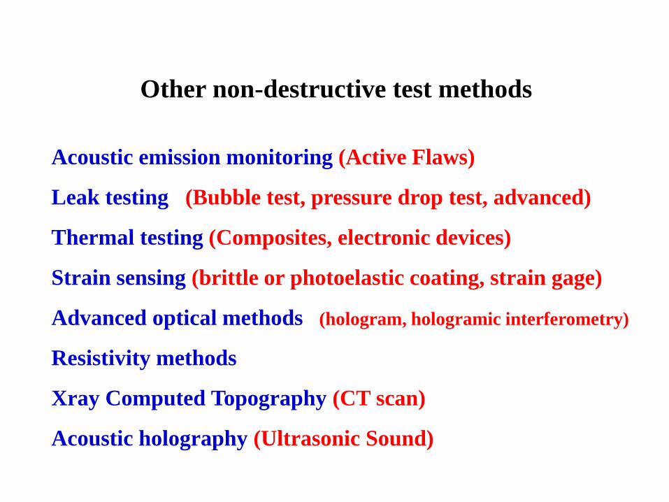
Acoustic emission monitoring (Active Flaws)

Leak testing (Bubble test, pressure drop test, advanced)

Thermal testing (Composites, electronic devices)

Strain sensing (brittle or photoelastic coating, strain gage)

Advanced optical methods (hologram, hologramic interferometry)

Resistivity methods

Xray Computed Topography (CT scan)

Acoustic holography (Ultrasonic Sound)

Other non-destructive test methods

Process Capability and Quality

Control

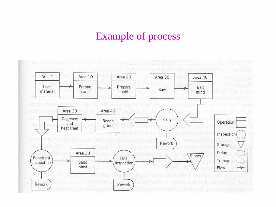
Example of process

Process Capability and Quality Control

Any process exhibit a level of inherent variability

inherent capability

Process Capability : Ability of the process to yield consistently

the aimed output.

How to measure/quantify the Process Capability (PC)?

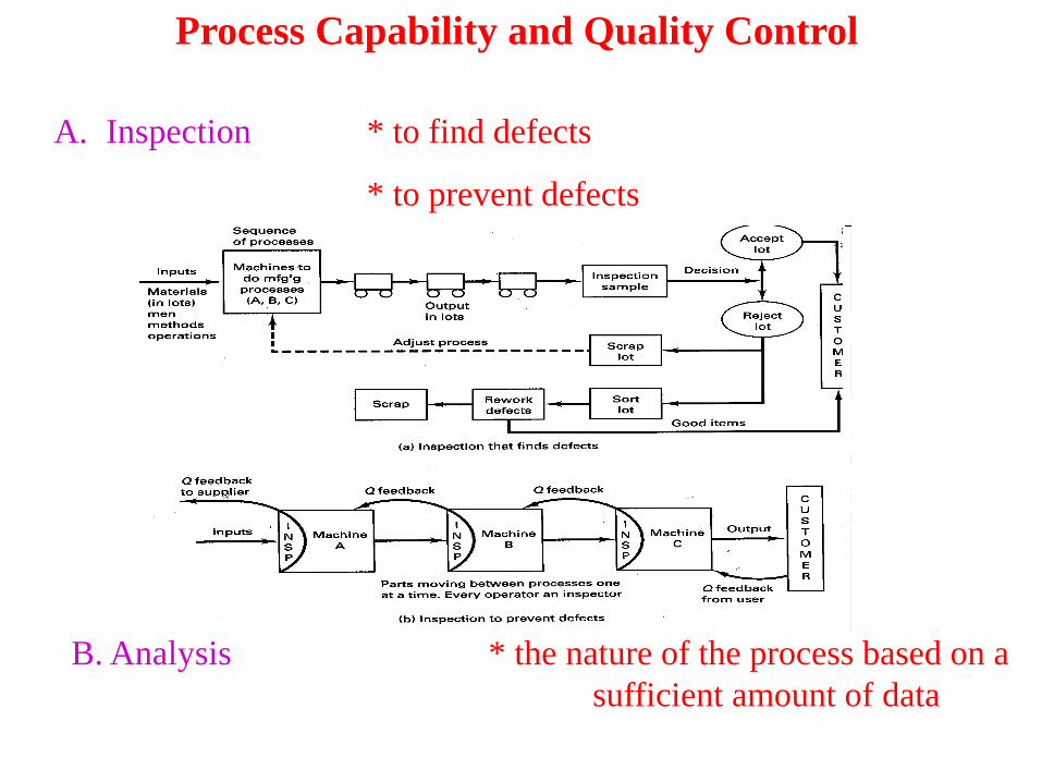
Process Capability and Quality Control

A. Inspection * to find defects

* to prevent defects

B. Analysis * the nature of the process based on a

sufficient amount of data

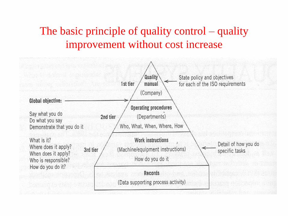
The basic principle of quality control – quality

improvement without cost increase

Steps to take:

1) Design an experiment ( machine, setting, speeds,

cutting rates, feed, material etc.)

2) Define the inspection method

3) Define the sample size

4) Separate parameters from noise

5) Take measurements

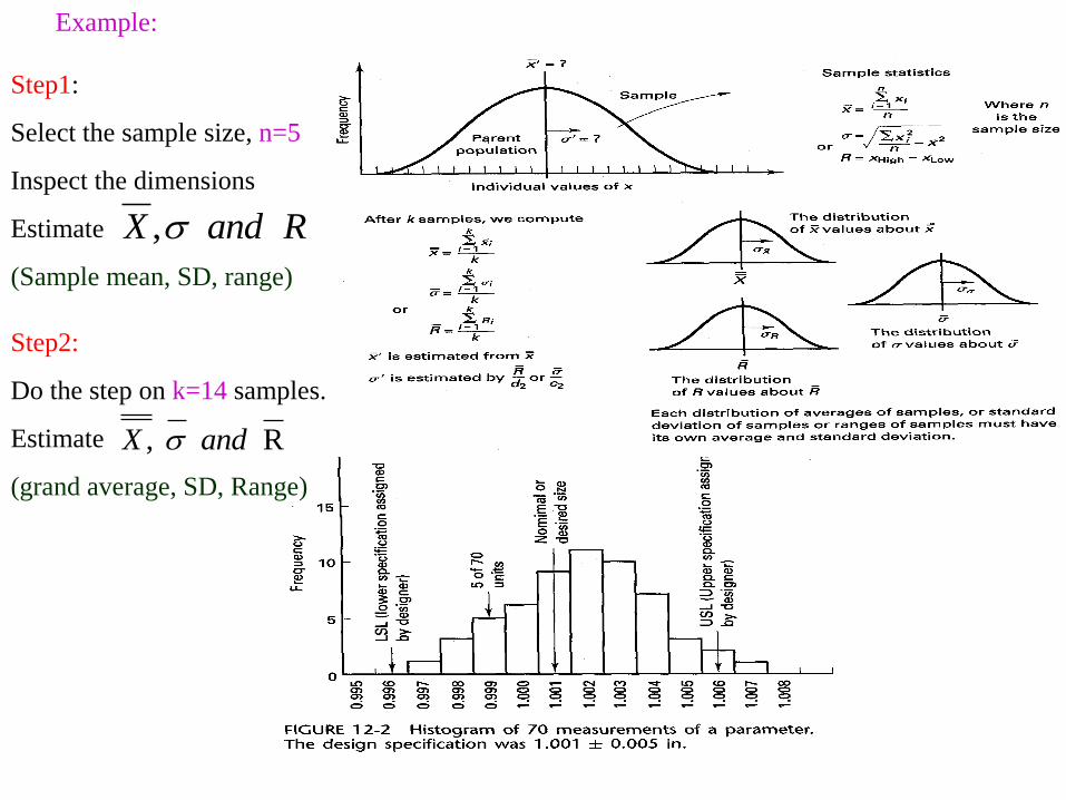
Example:

Step1:

Select the sample size, n=5

Inspect the dimensions

Estimate

(Sample mean, SD, range)

RandX ,

Step2:

Do the step on k=14 samples.

Estimate

(grand average, SD, Range)

R , andX

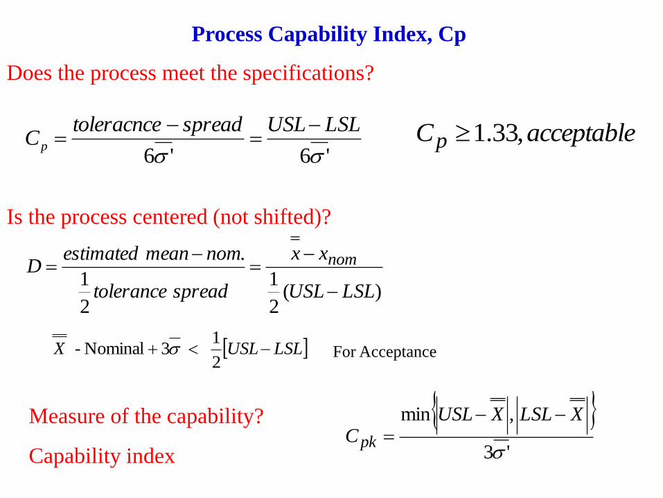
Does the process meet the specifications?

'6'6

LSLUSLspreadtoleracnceCp

acceptableCp ,33.1

Is the process centered (not shifted)?

)(2

1

2

1

.

LSLUSL

xx

spreadtolerance

nommeanestimatedD nom

Measure of the capability?

Capability index

'3

,min

XLSLXUSLCpk

Process Capability Index, Cp

LSLUSLX 2

1 3 Nominal - For Acceptance

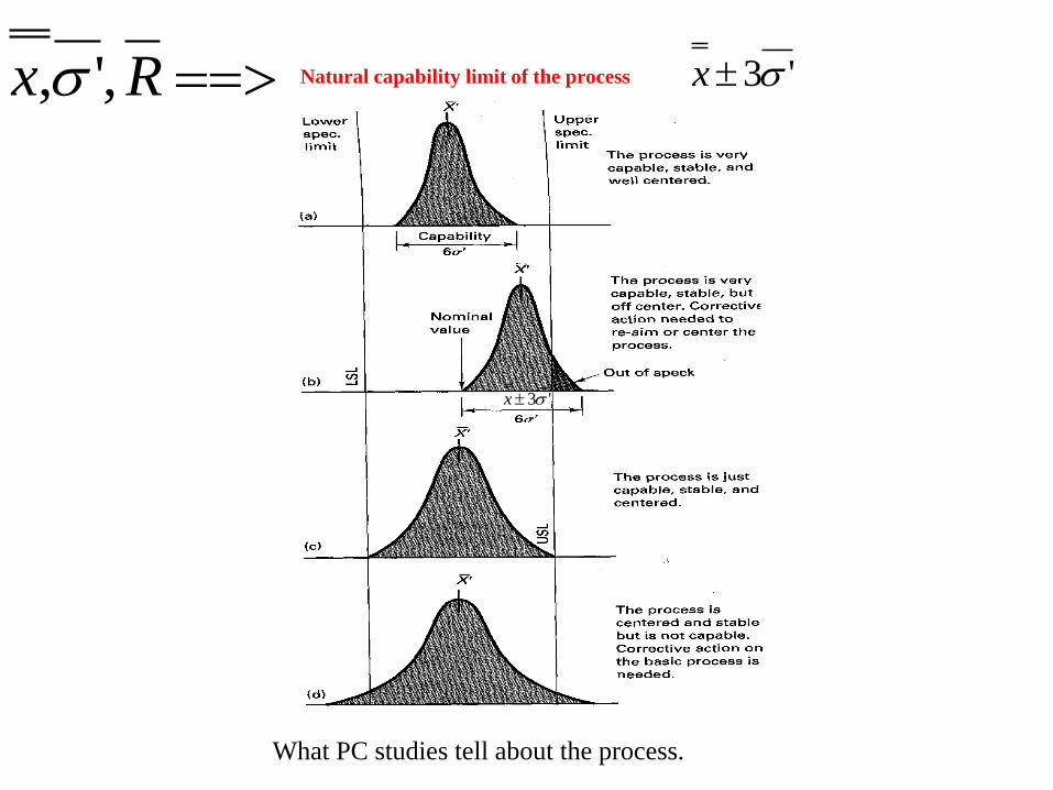
'3x

Rx ,', Natural capability limit of the process '3x

What PC studies tell about the process.

2

'

c

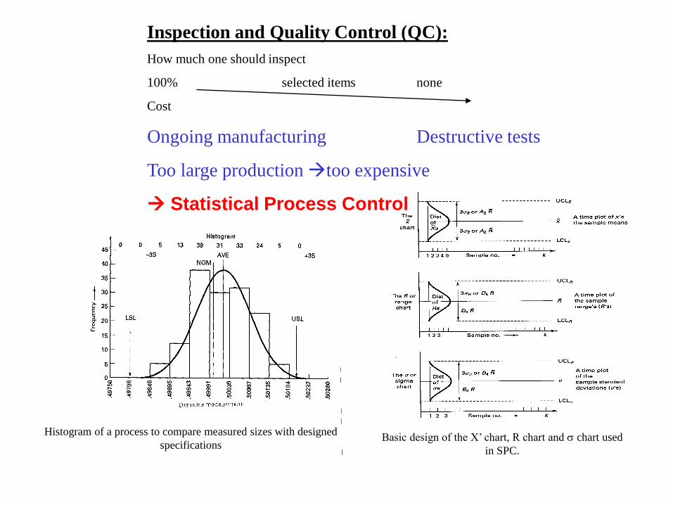
Inspection and Quality Control (QC):

How much one should inspect

100% selected items none

Cost

Ongoing manufacturing Destructive tests

Too large production too expensive

Statistical Process Control

Histogram of a process to compare measured sizes with designed

specificationsBasic design of the X’ chart, R chart and chart used

in SPC.

Six Sigma Model

USL-LSL 12

'6x

68.26%

2 95.46%

3 99.73% 7 out of 10,000

6 99.9999 3.4 ppm

How a process can get out of control?1. Wear

2. Inherent errors

3. Heating

4. Vibrations

5. Fault measurement/settings

Solutions:

Shift the job

Relax the specs

Sort the products

Improve precision:

switch the cutting tool switch the work holding device

change the material overhaul the process

find (eliminate cause of variability)

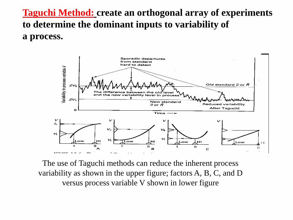
Taguchi Method: create an orthogonal array of experiments

to determine the dominant inputs to variability of

a process.

The use of Taguchi methods can reduce the inherent process

variability as shown in the upper figure; factors A, B, C, and D

versus process variable V shown in lower figure

Quality Control Charts:

Statistical quality control charts

for 12.700mm (0.5000-in.)-

diameter pins. Note the trend in

the X’ curve before the tool

change, indicating that the

mean was shifting due to tool

wear.

UCL- upper control limit

LCL-lower control limit RAxxx 2'3

RAxxx 2'3

Samples of Chart Patterns

Examples of X’ control charts

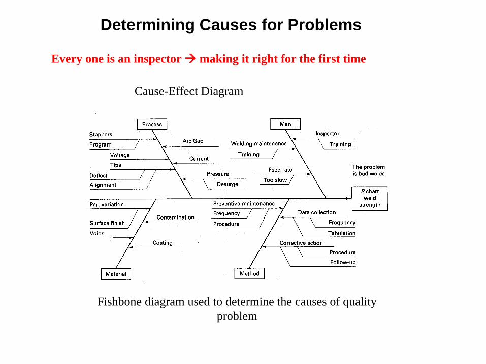
Fishbone diagram used to determine the causes of quality

problem

Determining Causes for Problems

Cause-Effect Diagram

Every one is an inspector making it right for the first time

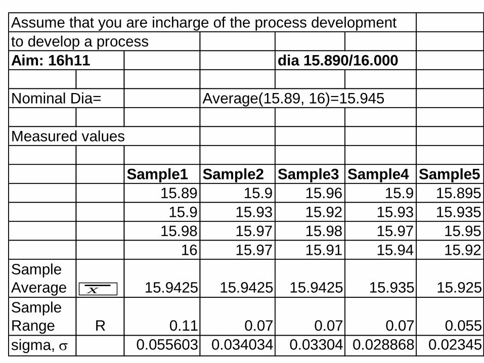
Assume that you are incharge of the process development

to develop a process

Aim: 16h11 dia 15.890/16.000

Nominal Dia= Average(15.89, 16)=15.945

Measured values

Sample1 Sample2 Sample3 Sample4 Sample5

15.89 15.9 15.96 15.9 15.895

15.9 15.93 15.92 15.93 15.935

15.98 15.97 15.98 15.97 15.95

16 15.97 15.91 15.94 15.92

Sample

Average 15.9425 15.9425 15.9425 15.935 15.925

Sample

Range R 0.11 0.07 0.07 0.07 0.055

sigma, 0.055603 0.034034 0.03304 0.028868 0.02345

X

15.9375

0.075

0.034999

4

XX

4 R

R

Fig.12.13in given are A2 and d2

5n

0548.0075.0*73.03 3

2

2

where

d

RRA

n

x

883.15055.0938.153

993.15055.0938.153

x

x

XLCLx

XUCLx

0075.0*0

171.0075.0*28.2

3

4

RDLCL

RDUCL

R

R

4

4 8.02 0438.08.0

035.0

2 '

nforcasc

USL= 16.000

LSL= 15.890

0.418569

0.361491629

'6

Cp

LSLUSL

034.0)89.1516(2

9375.15945.15

)(2D

LSLUSL

XXnom

'3

,min

XLSLXUSLCpk

Is the process ACCEPTABLE?

X Bar Variation

15.86

15.88

15.9

15.92

15.94

15.96

15.98

16

16.02

0 1 2 3 4 5 6

Sample #

X B

ar

UCLx

LCLx

Actual Mean

Nominal

LSL

USL

R Variation

0

0.02

0.04

0.06

0.08

0.1

0.12

0.14

0.16

0.18

0 1 2 3 4 5 6

Sample #

R

LCLR

Grand R

Sample R

LCLR

Find Cp, D and Cpk