Download - 3. VEHICLE-MOUNTED GPR SYSTEM FOR LANDMINE DETECTIONmagnet.cneas.tohoku.ac.jp/satolab/theses/kazunoriPhDThesis/Chapt… · 3. VEHICLE-MOUNTED GPR SYSTEM FOR LANDMINE DETECTION 3.1

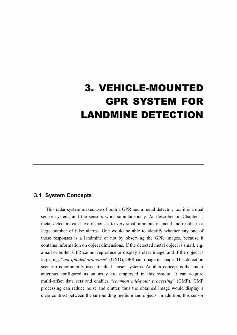
3. VEHICLE-MOUNTED GPR SYSTEM FOR

LANDMINE DETECTION

3.1 System Concepts

This radar system makes use of both a GPR and a metal detector, i.e., it is a dual sensor system, and the sensors work simultaneously. As described in Chapter 1, metal detectors can have responses to very small amounts of metal and results in a large number of false alarms. One would be able to identify whether any one of those responses is a landmine or not by observing the GPR images, because it contains information on object dimensions. If the detected metal object is small, e.g. a nail or bullet, GPR cannot reproduce or display a clear image, and if the object is large, e.g. “unexploded ordinance” (UXO), GPR can image its shape. This detection scenario is commonly used for dual sensor systems. Another concept is that radar antennas configured as an array are employed in this system. It can acquire multi-offset data sets and enables “common mid-point processing” (CMP). CMP processing can reduce noise and clutter, thus the obtained image would display a clear contrast between the surrounding medium and objects. In addition, this sensor

28 3. Vehicle-Mounted GPR System for Landmine Detection

is scanned by a robot arm mechanically. Hence, data quality would be stable, and the sensor can be scanned automatically resulting in the system to become of high efficiency. The goal is for the surveying time including data acquisition, processing, and interpretation to be within 10 minutes for 1 sq. m.

The image reconstruction uses synthetic aperture radar (SAR) technology, thus the system is named SAR-GPR. The development of SAR-GPR is under a program “Research and Development of Sensing Technology, Access and Control Technology to Support Humanitarian Demining of Antipersonnel Mines” founded by Japanese Science and Technology Agency (JST), which the competent authority is Ministry of Education, Culture, Sports, Science and Technology (MEXT).

3.2 Development of the System

3.2.1 Hardware configuration

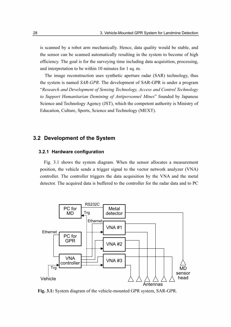
Fig. 3.1 shows the system diagram. When the sensor allocates a measurement position, the vehicle sends a trigger signal to the vector network analyzer (VNA) controller. The controller triggers the data acquisition by the VNA and the metal detector. The acquired data is buffered to the controller for the radar data and to PC

VNA #1

VNA #2

VNA #3VNAcontroller

PC forGPR

PC forMD

MetaldetectorTrg

Ethernet

Vehicle

Ethernet

RS232C

Trg

Antennas

MDsensorhead

Fig. 3.1: System diagram of the vehicle-mounted GPR system, SAR-GPR.

3.2 Development of the System 29

for the metal detector data. The system is a vector network analyzer based radar system, i.e., it is a stepped-frequency radar system. The reason why this type of radar system is employed is that the most critical parameter to investigate subsurface object is the operating frequency range, and it can easily be changed in a stepped-frequency radar system.

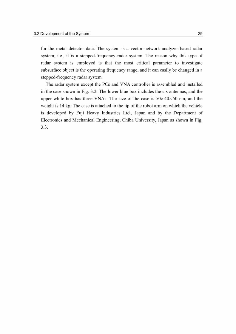
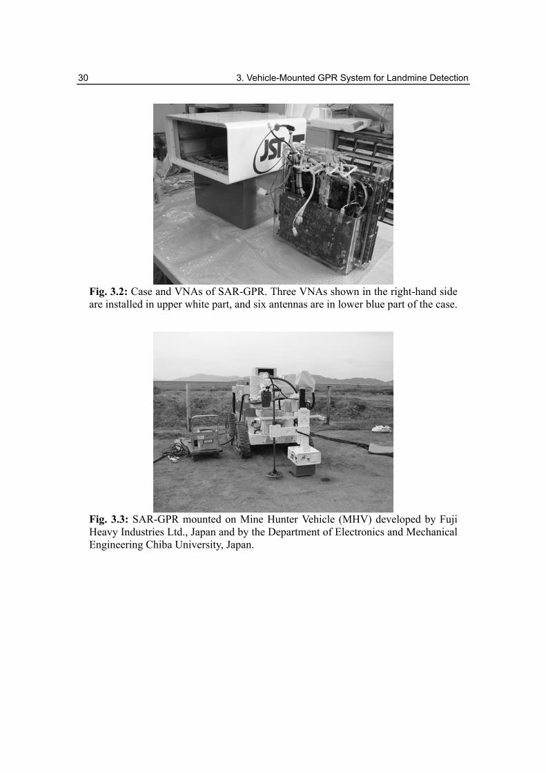
The radar system except the PCs and VNA controller is assembled and installed in the case shown in Fig. 3.2. The lower blue box includes the six antennas, and the upper white box has three VNAs. The size of the case is 50×40×50 cm, and the weight is 14 kg. The case is attached to the tip of the robot arm on which the vehicle is developed by Fuji Heavy Industries Ltd., Japan and by the Department of Electronics and Mechanical Engineering, Chiba University, Japan as shown in Fig. 3.3.


Fig. 3.2: Case and VNAs of SAR-GPR. Three VNAs shown in the right-hand side are installed in upper white part, and six antennas are in lower blue part of the case.

Fig. 3.3: SAR-GPR mounted on Mine Hunter Vehicle (MHV) developed by Fuji Heavy Industries Ltd., Japan and by the Department of Electronics and Mechanical Engineering Chiba University, Japan.


3.2.2 Use of three VNAs

In this system, three pairs of antennas are used to acquire multi-offset data. In general GPR measurements of geological surveys, the data acquisition is done over and over again with changing the separation of antennas or with switching the signal using array antennas. However, the acquisition must be done three times for one position and the goal cannot be accomplished by using these methods. Our solution is simultaneous usage of three vector network analyzers. This manner can ideally reduce the acquisition time by 1/3 compared to the case of using only one VNA.

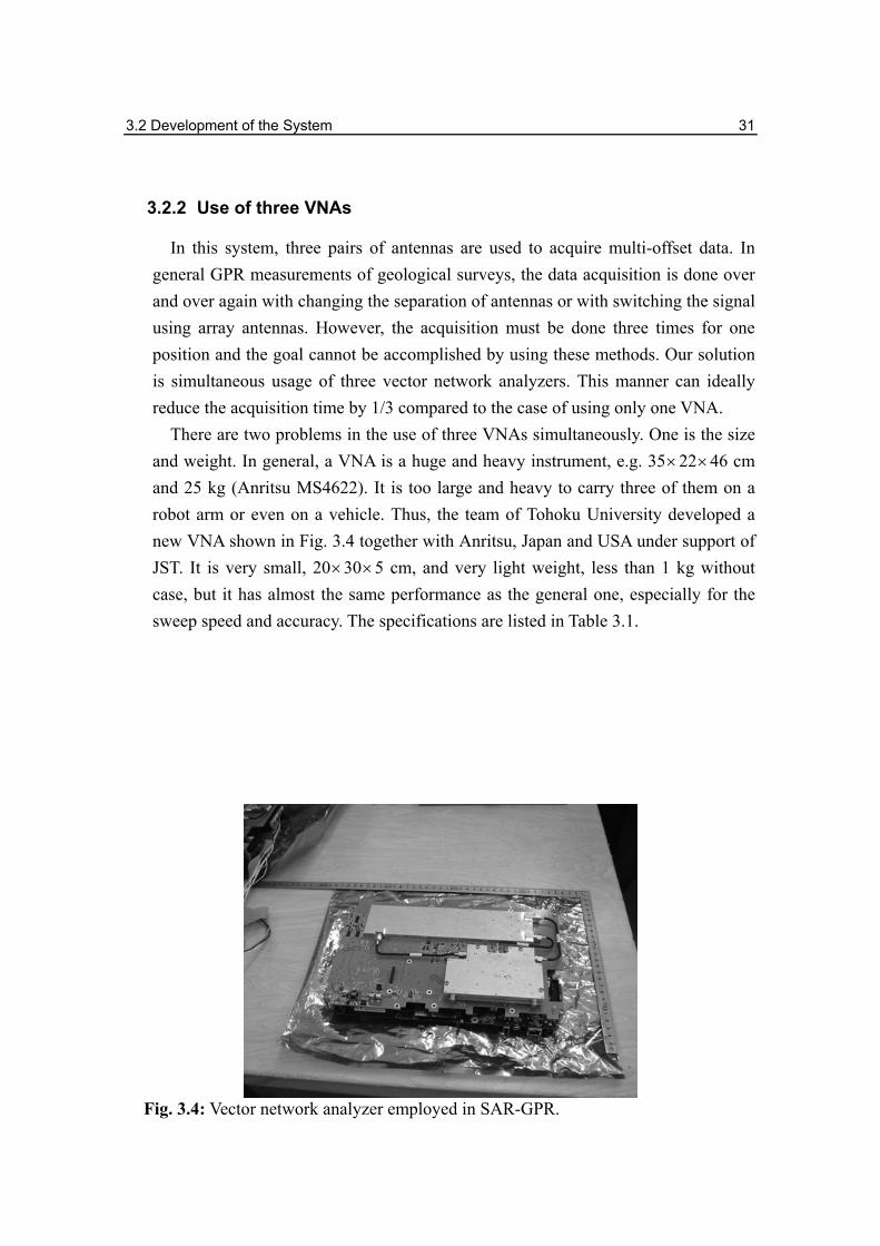
There are two problems in the use of three VNAs simultaneously. One is the size and weight. In general, a VNA is a huge and heavy instrument, e.g. 35×22×46 cm and 25 kg (Anritsu MS4622). It is too large and heavy to carry three of them on a robot arm or even on a vehicle. Thus, the team of Tohoku University developed a new VNA shown in Fig. 3.4 together with Anritsu, Japan and USA under support of JST. It is very small, 20×30×5 cm, and very light weight, less than 1 kg without case, but it has almost the same performance as the general one, especially for the sweep speed and accuracy. The specifications are listed in Table 3.1.

Fig. 3.4: Vector network analyzer employed in SAR-GPR.


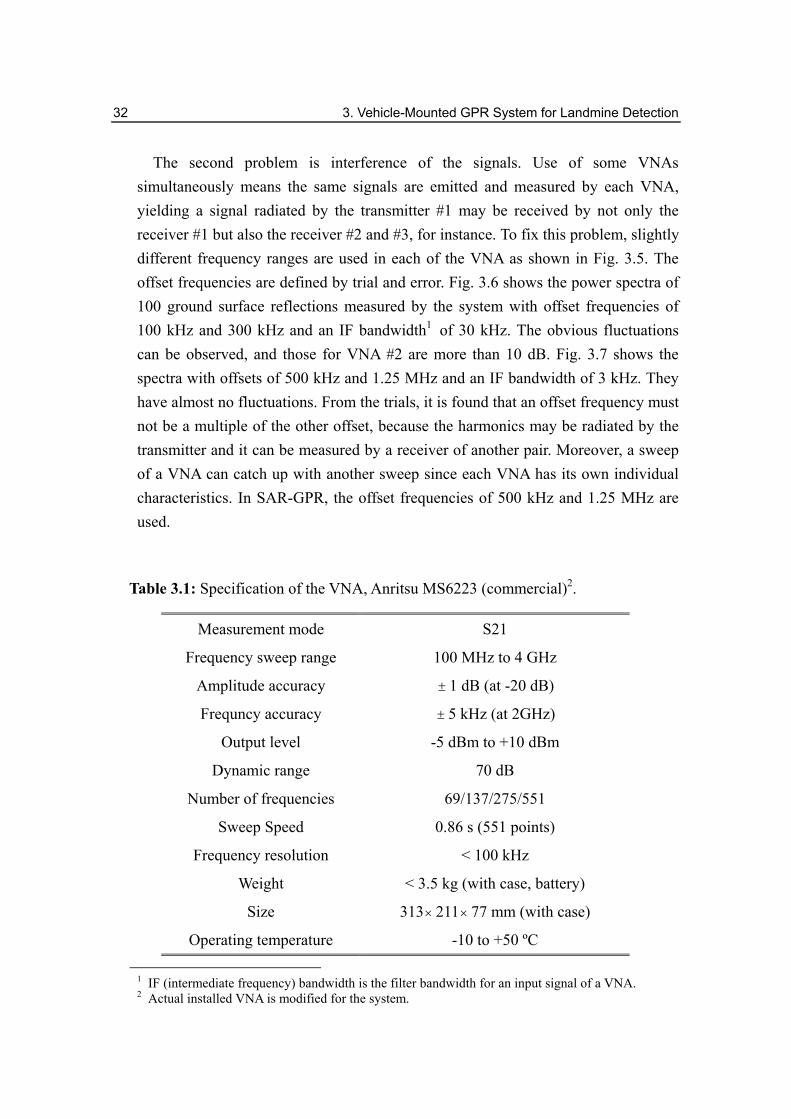
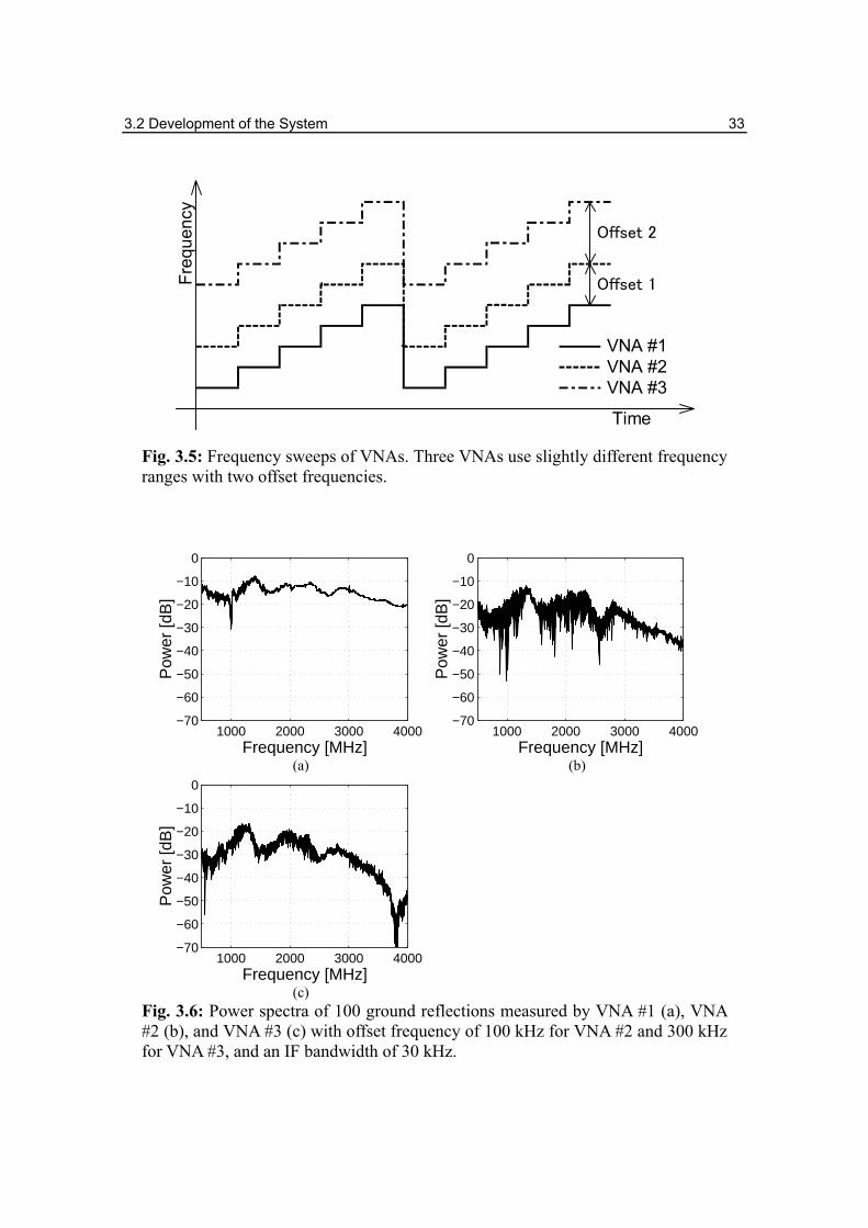
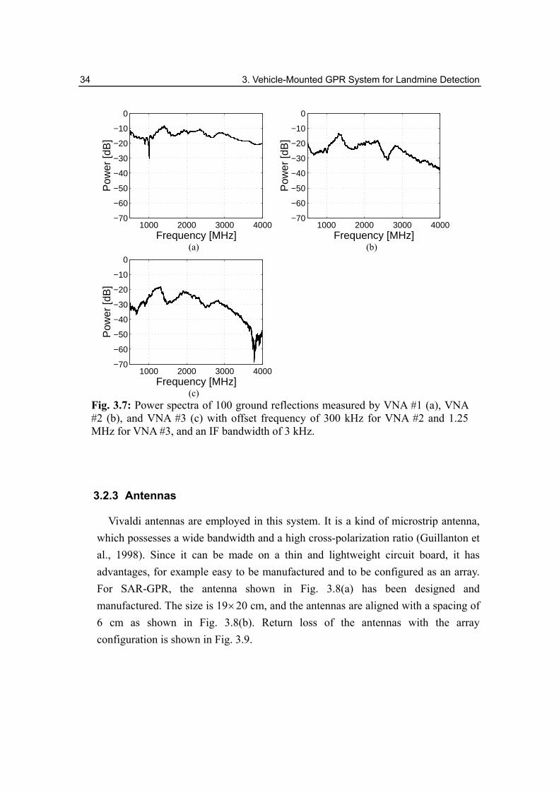
The second problem is interference of the signals. Use of some VNAs simultaneously means the same signals are emitted and measured by each VNA, yielding a signal radiated by the transmitter #1 may be received by not only the receiver #1 but also the receiver #2 and #3, for instance. To fix this problem, slightly different frequency ranges are used in each of the VNA as shown in Fig. 3.5. The offset frequencies are defined by trial and error. Fig. 3.6 shows the power spectra of 100 ground surface reflections measured by the system with offset frequencies of 100 kHz and 300 kHz and an IF bandwidth1 of 30 kHz. The obvious fluctuations can be observed, and those for VNA #2 are more than 10 dB. Fig. 3.7 shows the spectra with offsets of 500 kHz and 1.25 MHz and an IF bandwidth of 3 kHz. They have almost no fluctuations. From the trials, it is found that an offset frequency must not be a multiple of the other offset, because the harmonics may be radiated by the transmitter and it can be measured by a receiver of another pair. Moreover, a sweep of a VNA can catch up with another sweep since each VNA has its own individual characteristics. In SAR-GPR, the offset frequencies of 500 kHz and 1.25 MHz are used.

Table 3.1: Specification of the VNA, Anritsu MS6223 (commercial)2.

Measurement mode S21

Frequency sweep range 100 MHz to 4 GHz

Amplitude accuracy ± 1 dB (at -20 dB)

Frequncy accuracy ± 5 kHz (at 2GHz)

Output level -5 dBm to +10 dBm

Dynamic range 70 dB

Number of frequencies 69/137/275/551

Sweep Speed 0.86 s (551 points)

Frequency resolution < 100 kHz

Weight < 3.5 kg (with case, battery)

Size 313× 211× 77 mm (with case)

Operating temperature -10 to +50 ºC

1 IF (intermediate frequency) bandwidth is the filter bandwidth for an input signal of a VNA. 2 Actual installed VNA is modified for the system.


Time

Freq

uenc

y

VNA #1VNA #2VNA #3

Offset 1

Offset 2

Fig. 3.5: Frequency sweeps of VNAs. Three VNAs use slightly different frequency ranges with two offset frequencies.

1000 2000 3000 4000−70

−60

−50

−40

−30

−20

−10

0

Frequency [MHz]

Pow

er [d

B]

1000 2000 3000 4000

−70

−60

−50

−40

−30

−20

−10

0

Frequency [MHz]

Pow

er [d

B]

(a) (b)

1000 2000 3000 4000−70

−60

−50

−40

−30

−20

−10

0

Frequency [MHz]

Pow

er [d

B]

(c)

Fig. 3.6: Power spectra of 100 ground reflections measured by VNA #1 (a), VNA #2 (b), and VNA #3 (c) with offset frequency of 100 kHz for VNA #2 and 300 kHz for VNA #3, and an IF bandwidth of 30 kHz.


1000 2000 3000 4000−70

−60

−50

−40

−30

−20

−10

0

Frequency [MHz]

Pow

er [d

B]

1000 2000 3000 4000

−70

−60

−50

−40

−30

−20

−10

0

Frequency [MHz]

Pow

er [d

B]

(a) (b)

1000 2000 3000 4000−70

−60

−50

−40

−30

−20

−10

0

Frequency [MHz]

Pow

er [d

B]

(c)

Fig. 3.7: Power spectra of 100 ground reflections measured by VNA #1 (a), VNA #2 (b), and VNA #3 (c) with offset frequency of 300 kHz for VNA #2 and 1.25 MHz for VNA #3, and an IF bandwidth of 3 kHz.

3.2.3 Antennas

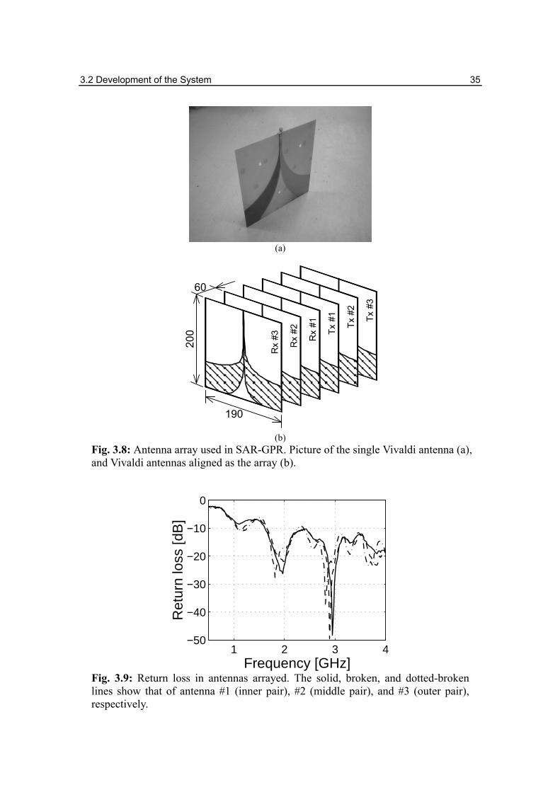
Vivaldi antennas are employed in this system. It is a kind of microstrip antenna, which possesses a wide bandwidth and a high cross-polarization ratio (Guillanton et al., 1998). Since it can be made on a thin and lightweight circuit board, it has advantages, for example easy to be manufactured and to be configured as an array. For SAR-GPR, the antenna shown in Fig. 3.8(a) has been designed and manufactured. The size is 19×20 cm, and the antennas are aligned with a spacing of 6 cm as shown in Fig. 3.8(b). Return loss of the antennas with the array configuration is shown in Fig. 3.9.


(a)

200

60

190

Rx

#1

Tx #

1

Tx #

2

Tx #

3

Rx

#2

Rx

#3

(b)

Fig. 3.8: Antenna array used in SAR-GPR. Picture of the single Vivaldi antenna (a), and Vivaldi antennas aligned as the array (b).

1 2 3 4−50

−40

−30

−20

−10

0

Frequency [GHz]

Ret

urn

loss

[dB

]

Fig. 3.9: Return loss in antennas arrayed. The solid, broken, and dotted-broken lines show that of antenna #1 (inner pair), #2 (middle pair), and #3 (outer pair), respectively.


3.3 Image Reconstruction

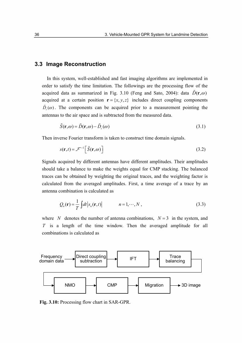
In this system, well-established and fast imaging algorithms are implemented in order to satisfy the time limitation. The followings are the processing flow of the acquired data as summarized in Fig. 3.10 (Feng and Sato, 2004): data ( , )D ωr acquired at a certain position { , , }x y z=r includes direct coupling components

( )cD ω . The components can be acquired prior to a measurement pointing the antennas to the air space and is subtracted from the measured data.

( , ) ( , ) ( )cS D Dω ω ω= −r r (3.1)

Then inverse Fourier transform is taken to construct time domain signals.

1( , ) ( , )s t S ω− = r rF (3.2)

Signals acquired by different antennas have different amplitudes. Their amplitudes should take a balance to make the weights equal for CMP stacking. The balanced traces can be obtained by weighting the original traces, and the weighting factor is calculated from the averaged amplitudes. First, a time average of a trace by an antenna combination is calculated as

1( ) ( , ) 1, ,n nQ dt s t n NT

= =∫r r , (3.3)

where N denotes the number of antenna combinations, 3N = in the system, and T is a length of the time window. Then the averaged amplitude for all combinations is calculated as

Direct couplingsubtraction

NMO CMP

Frequencydomain data IFT

Migration 3D image

Tracebalancing

Fig. 3.10: Processing flow chart in SAR-GPR.

3.3 Image Reconstruction 37

1

1( ) ( )N

nn

Q QN =

= ∑r r . (3.4)

According to Eqs. (3.3) and (3.4), the weighting factor is defined as the ratio

( )( )( )n

n

QWQ

=rrr

(3.5)

With the weighting factor, the balanced traces ˆ( , )s tr are calculated as

ˆ ( , ) ( , ) ( )n n ns t s t W= ⋅r r r . (3.6)

Next, these traces for each antenna combination are stacked to reduce incoherent clutter and noise. Since these traces have different offset (antenna separation), their time axes are not the same. To compensate the axes, normal move out (NMO) is performed, and then the traces are stacked.

1

ˆ( , ) ( , )N

CMP n nn

s t s τ=

=∑r r , (3.7a)

where

21

air soiln n

nL Lc

τε

= +

, (3.7b)

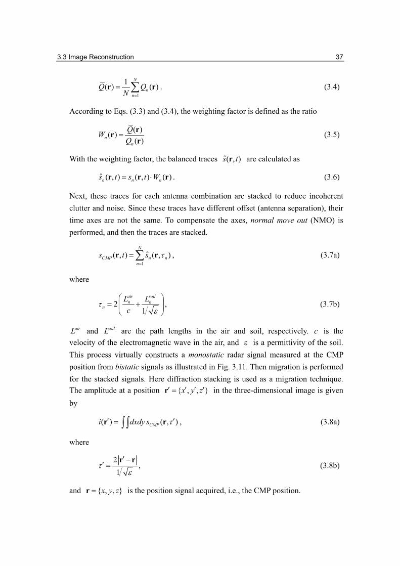
airL and soilL are the path lengths in the air and soil, respectively. c is the velocity of the electromagnetic wave in the air, and ε is a permittivity of the soil. This process virtually constructs a monostatic radar signal measured at the CMP position from bistatic signals as illustrated in Fig. 3.11. Then migration is performed for the stacked signals. Here diffraction stacking is used as a migration technique. The amplitude at a position { , , }x y z′ ′ ′ ′=r in the three-dimensional image is given by

( ) ( , )CMPi dxdy s τ′ ′= ∫ ∫r r , (3.8a)

where

21

τε

′ −′ =

r r, (3.8b)

and { , , }x y z=r is the position signal acquired, i.e., the CMP position.


Tx1TxN Rx1 RxNCMP

Lair

Lsoil

Fig. 3.11: Concept of CMP stacking. It constructs a virtual monostatic radar signal measured at the CMP point.

3.4 Quick Detection Algorithm

In general, landmines are found out from the GPR images by carefully checking the slices with changing the depths. It requires knowledge and experiences and is time consuming. Since actual demining operations will be done by non-specialists of GPR, the interpretation must not be complicated. Here a quick detection algorithm for landmines from GPR image is proposed. The algorithm is designed for the quick operation, and it permits that some number of false alarms may occur.

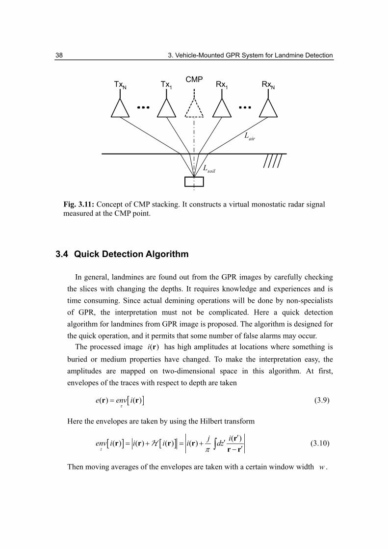
The processed image ( )i r has high amplitudes at locations where something is buried or medium properties have changed. To make the interpretation easy, the amplitudes are mapped on two-dimensional space in this algorithm. At first, envelopes of the traces with respect to depth are taken

[ ]( ) ( )z

e env i=r r (3.9)

Here the envelopes are taken by using the Hilbert transform

[ ] [ ] ( )( ) ( ) ( ) ( )z

j ienv i i i i dzπ

′′= + = +

′−∫rr r r r

r rH (3.10)

Then moving averages of the envelopes are taken with a certain window width w .

3.4 Quick Detection Algorithm 39

2

2

1( ) ( )z w

z we dz e

w′+

′−′ = ∫r r (3.11)

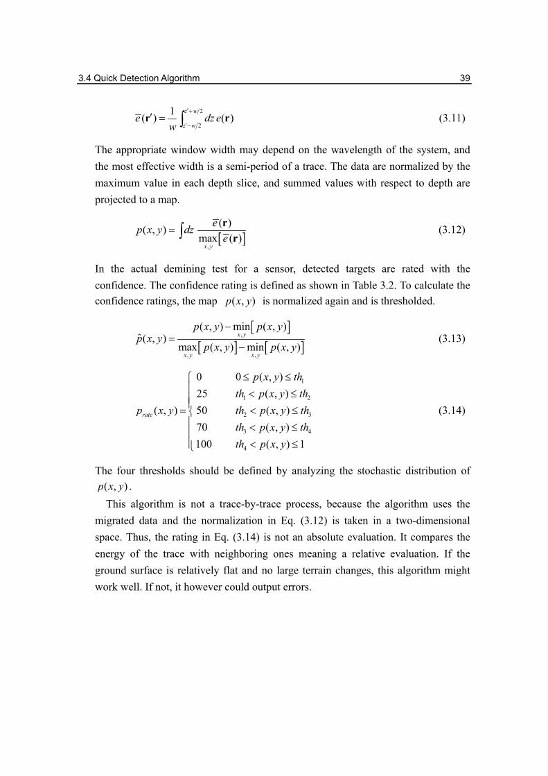
The appropriate window width may depend on the wavelength of the system, and the most effective width is a semi-period of a trace. The data are normalized by the maximum value in each depth slice, and summed values with respect to depth are projected to a map.

[ ],

( )( , )max ( )

x y

ep x y dze

= ∫r

r (3.12)

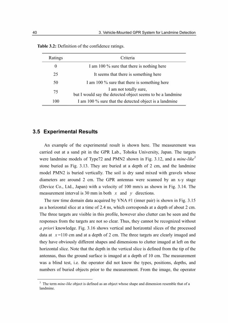
In the actual demining test for a sensor, detected targets are rated with the confidence. The confidence rating is defined as shown in Table 3.2. To calculate the confidence ratings, the map ( , )p x y is normalized again and is thresholded.

[ ][ ] [ ]

,

,,

( , ) min ( , )ˆ ( , )

max ( , ) min ( , )x y

x yx y

p x y p x yp x y

p x y p x y

−=

− (3.13)

1

1 2

2 3

3 4

4

0 0 ( , )25 ( , )

( , ) 50 ( , )70 ( , )100 ( , ) 1

rate

p x y thth p x y th

p x y th p x y thth p x y thth p x y

≤ ≤ < ≤= < ≤ < ≤ < ≤

(3.14)

The four thresholds should be defined by analyzing the stochastic distribution of ( , )p x y . This algorithm is not a trace-by-trace process, because the algorithm uses the

migrated data and the normalization in Eq. (3.12) is taken in a two-dimensional space. Thus, the rating in Eq. (3.14) is not an absolute evaluation. It compares the energy of the trace with neighboring ones meaning a relative evaluation. If the ground surface is relatively flat and no large terrain changes, this algorithm might work well. If not, it however could output errors.


Table 3.2: Definition of the confidence ratings.

Ratings Criteria

0 I am 100 % sure that there is nothing here

25 It seems that there is something here

50 I am 100 % sure that there is something here

75 I am not totally sure, but I would say the detected object seems to be a landmine

100 I am 100 % sure that the detected object is a landmine

3.5 Experimental Results

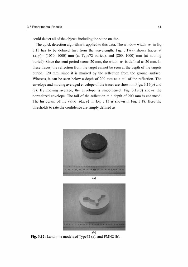
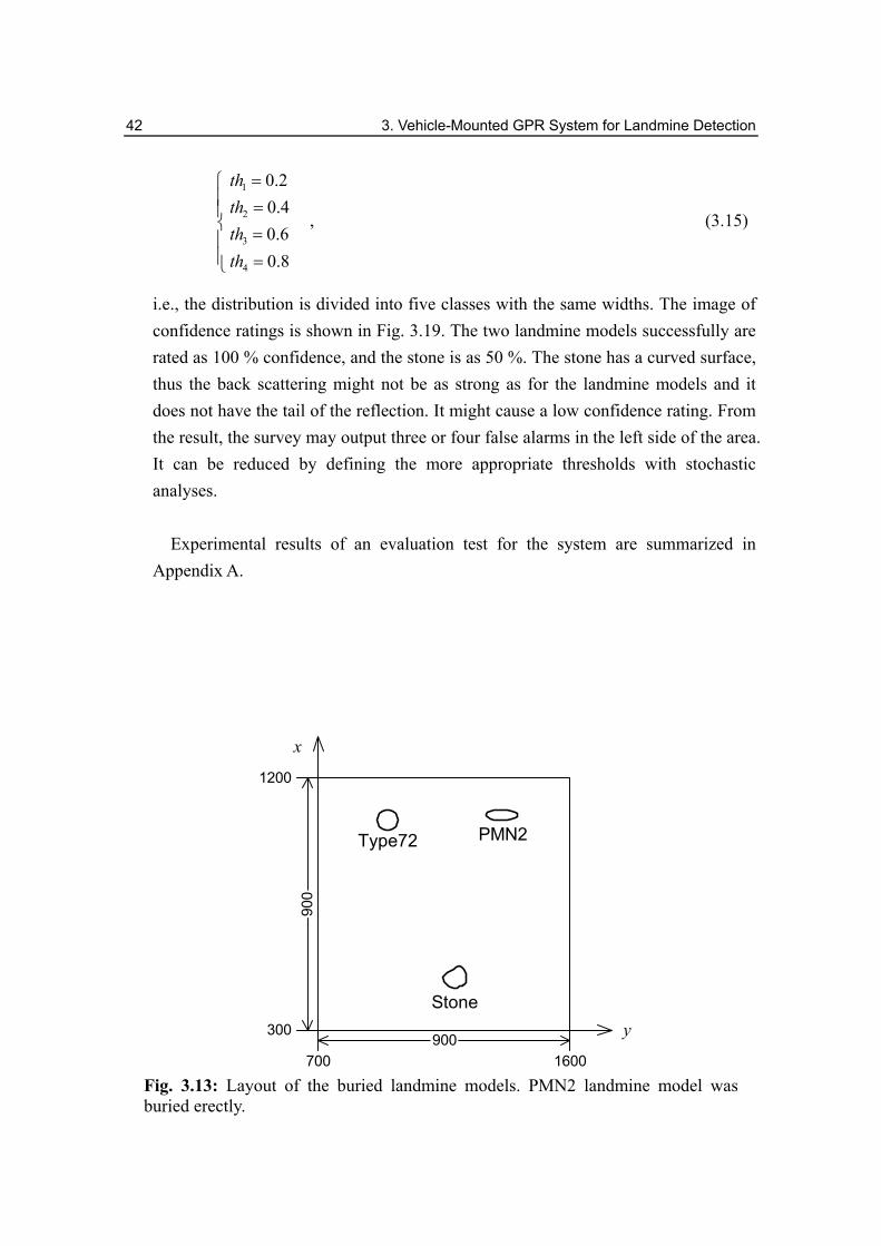
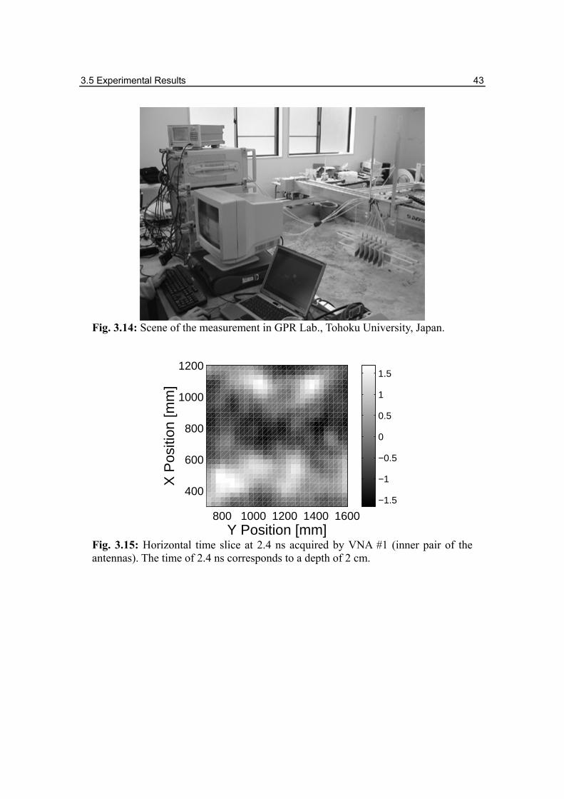
An example of the experimental result is shown here. The measurement was carried out at a sand pit in the GPR Lab., Tohoku University, Japan. The targets were landmine models of Type72 and PMN2 shown in Fig. 3.12, and a mine-like3 stone buried as Fig. 3.13. They are buried at a depth of 2 cm, and the landmine model PMN2 is buried vertically. The soil is dry sand mixed with gravels whose diameters are around 2 cm. The GPR antennas were scanned by an x-y stage (Device Co., Ltd., Japan) with a velocity of 100 mm/s as shown in Fig. 3.14. The measurement interval is 30 mm in both x and y directions.

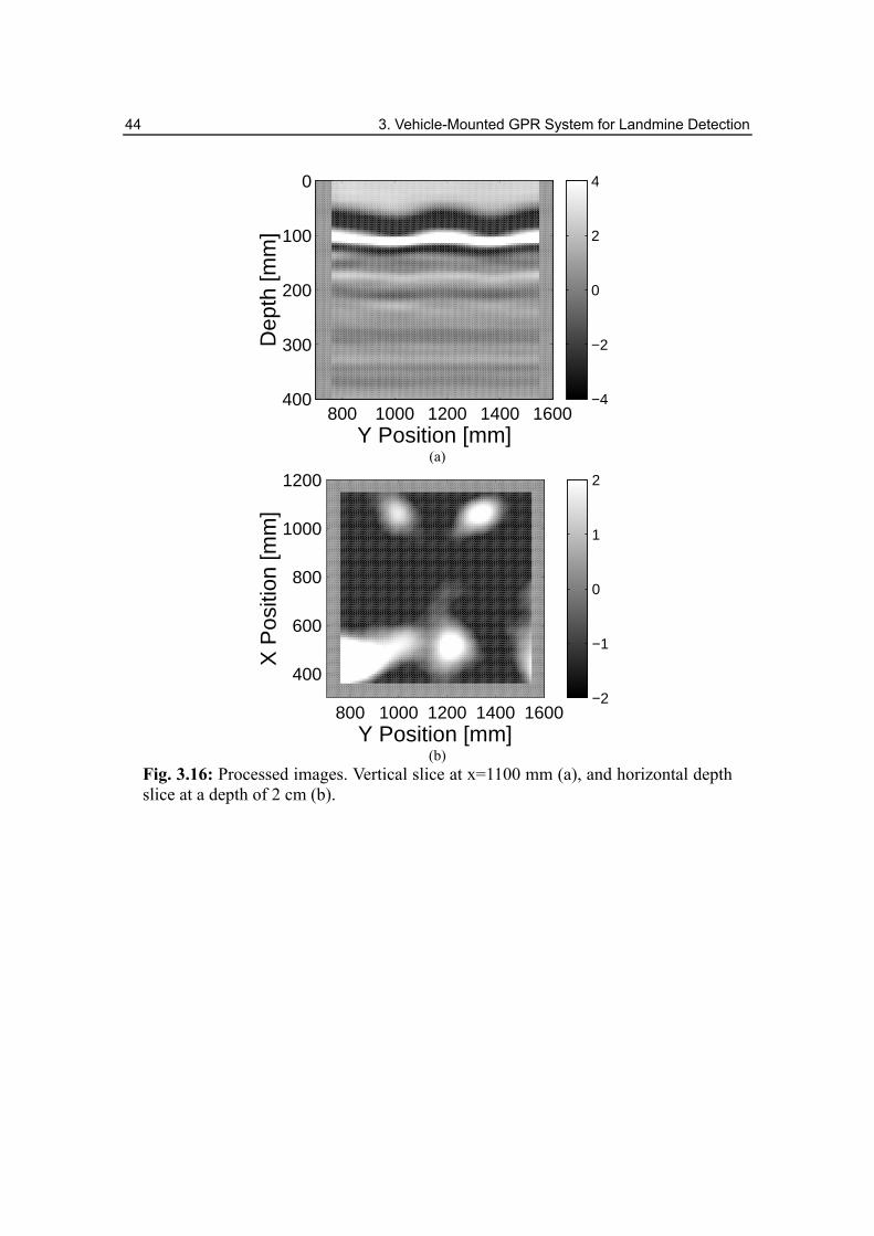
The raw time domain data acquired by VNA #1 (inner pair) is shown in Fig. 3.15 as a horizontal slice at a time of 2.4 ns, which corresponds at a depth of about 2 cm. The three targets are visible in this profile, however also clutter can be seen and the responses from the targets are not so clear. Thus, they cannot be recognized without a priori knowledge. Fig. 3.16 shows vertical and horizontal slices of the processed data at x =110 cm and at a depth of 2 cm. The three targets are clearly imaged and they have obviously different shapes and dimensions to clutter imaged at left on the horizontal slice. Note that the depth in the vertical slice is defined from the tip of the antennas, thus the ground surface is imaged at a depth of 10 cm. The measurement was a blind test, i.e. the operator did not know the types, positions, depths, and numbers of buried objects prior to the measurement. From the image, the operator

3 The term mine-like object is defined as an object whose shape and dimension resemble that of a landmine.

3.5 Experimental Results 41

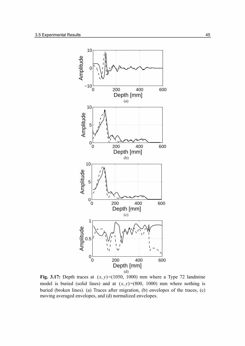
could detect all of the objects including the stone on site. The quick detection algorithm is applied to this data. The window width w in Eq.

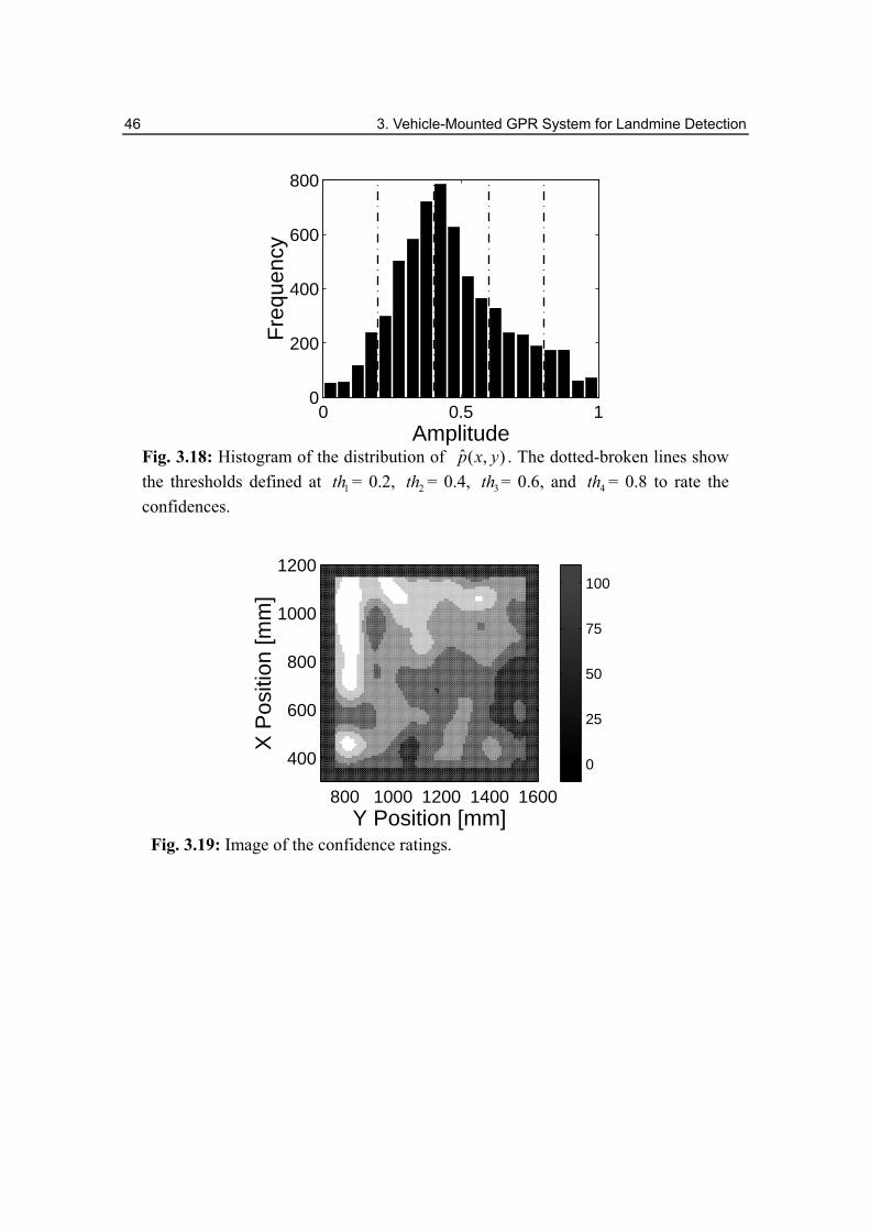
3.11 has to be defined first from the wavelength. Fig. 3.17(a) shows traces at ( , )x y = (1050, 1000) mm (at Type72 buried), and (800, 1000) mm (at nothing buried). Since the semi-period seems 20 mm, the width w is defined as 20 mm. In these traces, the reflection from the target cannot be seen at the depth of the targets buried, 120 mm, since it is masked by the reflection from the ground surface. Whereas, it can be seen below a depth of 200 mm as a tail of the reflection. The envelope and moving averaged envelope of the traces are shown in Figs. 3.17(b) and (c). By moving average, the envelope is smoothened. Fig. 3.17(d) shows the normalized envelope. The tail of the reflection at a depth of 200 mm is enhanced. The histogram of the value ˆ ( , )p x y in Eq. 3.13 is shown in Fig. 3.18. Here the thresholds to rate the confidence are simply defined as

(a)

(b)

Fig. 3.12: Landmine models of Type72 (a), and PMN2 (b).


1

2

3

4

0.20.40.60.8

thththth

= = = =

, (3.15)

i.e., the distribution is divided into five classes with the same widths. The image of confidence ratings is shown in Fig. 3.19. The two landmine models successfully are rated as 100 % confidence, and the stone is as 50 %. The stone has a curved surface, thus the back scattering might not be as strong as for the landmine models and it does not have the tail of the reflection. It might cause a low confidence rating. From the result, the survey may output three or four false alarms in the left side of the area. It can be reduced by defining the more appropriate thresholds with stochastic analyses.

Experimental results of an evaluation test for the system are summarized in Appendix A.

x

y

Type72 PMN2

Stone

900

900

700 1600

300

1200

Fig. 3.13: Layout of the buried landmine models. PMN2 landmine model was buried erectly.


Fig. 3.14: Scene of the measurement in GPR Lab., Tohoku University, Japan.

800 1000 1200 1400 1600

400

600

800

1000

1200

Y Position [mm]

X P

ositi

on [m

m]

−1.5

−1

−0.5

0

0.5

1

1.5

Fig. 3.15: Horizontal time slice at 2.4 ns acquired by VNA #1 (inner pair of the antennas). The time of 2.4 ns corresponds to a depth of 2 cm.


800 1000 1200 1400 1600

0

100

200

300

400

Y Position [mm]

Dep

th [m

m]

−4

−2

0

2

4

(a)

800 1000 1200 1400 1600

400

600

800

1000

1200

Y Position [mm]

X P

ositi

on [m

m]

−2

−1

0

1

2

(b)

Fig. 3.16: Processed images. Vertical slice at x=1100 mm (a), and horizontal depth slice at a depth of 2 cm (b).


0 200 400 600−10

0

10

Depth [mm]

Am

plitu

de

(a)

0 200 400 6000

5

10

Depth [mm]

Am

plitu

de

(b)

0 200 400 6000

5

10

Depth [mm]

Am

plitu

de

(c)

0 200 400 6000

0.5

1

Depth [mm]

Am

plitu

de

(d)

Fig. 3.17: Depth traces at ( , )x y =(1050, 1000) mm where a Type 72 landmine model is buried (solid lines) and at ( , )x y =(800, 1000) mm where nothing is buried (broken lines). (a) Traces after migration, (b) envelopes of the traces, (c) moving averaged envelopes, and (d) normalized envelopes.


0 0.5 10

200

400

600

800

Amplitude

Fre

quen

cy

Fig. 3.18: Histogram of the distribution of ˆ ( , )p x y . The dotted-broken lines show the thresholds defined at 1th = 0.2, 2th = 0.4, 3th = 0.6, and 4th = 0.8 to rate the confidences.

800 1000 1200 1400 1600

400

600

800

1000

1200

Y Position [mm]

X P

ositi

on [m

m]

0

25

50

75

100

Fig. 3.19: Image of the confidence ratings.