A functorial extension of the Magnus representationto the category of three-dimensional cobordisms

Vincent Florens Gwénaël Massuyeau Juan Serrano de Rodrigo

July 25, 2017

Abstract

Let R be an integral domain and G be a subgroup of its group of units. We considerthe category CobG of 3-dimensional cobordisms between oriented surfaces with connectedboundary, equipped with a representation of their fundamental group in G. Under somemild conditions on R, we construct a monoidal functor from CobG to the category pLagrRconsisting of “pointed Lagrangian relations” between skew-Hermitian R-modules. We call itthe “Magnus functor” since it contains the Magnus representation of mapping class groupsas a special case. Our construction is inspired from the work of Cimasoni and Turaev on theextension of the Burau representation of braid groups to the category of tangles. It can alsobe regarded as a G-equivariant version of a TQFT-like functor that has been described byDonaldson. The study and computation of the Magnus functor is carried out using classicaltechniques of low-dimensional topology. When G is a free abelian group and R = Z[G] is thegroup ring of G, we relate the Magnus functor to the “Alexander functor” (which has beenintroduced in a prior work using Alexander-type invariants), and we deduce a factorizationformula for the latter.

1 Introduction

Let Σ be a compact connected oriented surface with ∂Σ 6= ∅, and let π := π1(Σ, ?) be itsfundamental group based at a point ? ∈ ∂Σ. The mapping class group MCG(Σ) consists ofthe isotopy classes of (orientation-preserving) self-homeomorphisms of Σ fixing the boundarypointwise. “Magnus representations” usually refer to those “representations” of subgroups ofMCG(Σ) that are defined by assigning to an f ∈ MCG(Σ) the matrix with entries in Z[π]consisting of Fox’s free derivatives of f∗ : π → π with respect to a fixed basis of π. Thus theyhave a group-theoretical definition, which goes through the automorphism group of π.

Birman coined the terminology “Magnus representations” in the third chapter of her book [Bir74],where it is observed that these kinds of “representations” arise from matrix representations offree groups dating back to Magnus [Mag39]. Birman gave there an algebraic exposition andsurvey of these “representations”, explaining for instance how far they are from being grouphomomorphisms, or analyzing their kernels and images. One of her motivations was to give aunified treatment of the Burau representation of the braid group and the Gassner representationof the pure braid group. These correspond to the case where the surface Σ is a disk with markedpoints or holes, and are defined from the “Magnus representations” by reducing the coefficientsin Z[π] to some appropriate commutative rings.

1

arX

iv:1

604.

0690

5v4

[m

ath.

GT

] 2

4 Ju

l 201

7

The Gassner representation of the pure braid group was later extended to string links (also called“pure tangles”) by Le Dimet [LD92]. Kirk, Livingston and Wang [KLW01] gave a topologicalinterpretation of this extension and a simple proof of its invariance under concordance. Theirapproach is based on a natural action of the monoid of string links on the twisted homologyof a punctured disk, and relies on the topological interpretation of Fox’s free derivatives interms of universal covers. In these works, the study of the Burau and Gassner representationsis partly motivated by their tight connections with the Alexander polynomial of links. Morerecently, Cimasoni and Turaev [CT05, CT06] extended these representations to arbitrary tangles.Their invariant is defined as a functor from the category of (colored) tangles to the category of“Lagrangian relations” between skew-Hermitian modules.

In the case of a surface Σ of positive genus, Magnus representations have been used and studiedby Morita [Mor93], Suzuki [Suz03] and Perron [Per06] among others. In this case too, there is agroup-theoretical definition in terms of Fox’s free derivatives as well as a topological definitionusing twisted homology (see [Suz05]). Furthermore, the Magnus representation is extended in[Sak08] to the monoid of homology cobordisms (also called “homology cylinders”), which arehigher-genus versions of string links. In these works, the study of the Magnus representationis driven by its relations to the Alexander polynomial and Reidemeister torsions of closed 3-manifolds, and by its role in the study of the “Johnson homomorphisms”. We refer to Sakasai[Sak12] for an overview of these topics. In this paper, inspired by the above-mentioned work ofCimasoni and Turaev, we construct a functorial extension of the Magnus representations to acertain category of 3-dimensional cobordisms.

To be more specific, our framework is the category Cob of 3-dimensional cobordisms introducedby Crane and Yetter [CY99]. The objects of this category are compact connected orientedsurfaces Fg of arbitrary genus g ≥ 0, with exactly one boundary component, and the morphismsare 3-dimensional cobordisms with corners between such surfaces. The category Cob originatesfrom the study of 3-dimensional Topological Quantum Field Theories (TQFT’s). We considerhere the refinement CobG of this category where the surfaces and 3-manifolds are equipped witha representation of their fundamental group in a fixed group G.

Specifically, we assume that G is a subgroup of the group of units of an integral domain R, andthat R has an involutive ring endomorphism which extends the map of G given by g 7→ g−1.Recall from [CT05] that the category LagrR of Lagrangian relations is defined as follows: objectsare finitely generated R-modules H equipped with a non-degenerate skew-Hermitian form ρ,and morphisms (H1, ρ1) → (H2, ρ2) are Lagrangian submodules of

(H1 ⊕H2, (−ρ1)⊕ ρ2

). The

following construction can be regarded as a TQFT-like extension of the Magnus representations.

Theorem I. There exists a functor Mag := MagR,G : CobG → LagrR which is defined as follows.At the level of objects, Mag assigns to any pair

(Fg, ϕ : π1(Fg, ?) → G

)the skew-Hermitian

R-module (Hϕ

1 (Fg, ?), 〈·, ·〉s)

where ? ∈ ∂Fg and 〈·, ·〉s : Hϕ1 (Fg, ?)×Hϕ

1 (Fg, ?)→ R is a version of the equivariant intersectionform with coefficients in R twisted by ϕ. At the level of morphisms, Mag assigns to any cobordism(M,ϕ) between (Fg− , ϕ−) and (Fg+ , ϕ+) the (closure of) the kernel of the R-linear map

(−m−)⊕m+ : Hϕ−1 (Fg− , ?)⊕H

ϕ+

1 (Fg+ , ?) −→ Hϕ1 (M,?)

induced by the inclusions m± : Fg± → ∂M ⊂M .

2

One difficulty to adapt the work of Cimasoni and Turaev from tangles to cobordisms lies inthe construction of a skew-Hermitian form on Hϕ

1 (Fg, ?): here the form 〈·, ·〉s is derived fromthe homotopy intersection pairing that Turaev introduced in [Tur78]. The main advantageof considering the twisted homology of Fg relative to a base point ? (instead of the absolutetwisted homology as in [CT05]) is that the module associated to the surface Fg is always freeof rank 2g, regardless of the way coefficients are twisted by ϕ. Another difference with theirwork is that we will deal with monoidality. Indeed, the boundary-connected sums of surfacesand 3-manifolds induce a monoidal structure on the category CobG. We introduce the categorypLagrR of pointed Lagrangian relations where each skew-Hermitian R-module is endowed witha distinguished element of its rationalization. This refinement of the category LagrR has amonoidal structure defined by a skew version of the direct sum, and the above functor Magcan be refined to preserve these monoidal structures. (See Theorem 4.1 and Proposition 4.7 forprecise statements.) Apart for the aforesaid differences, the proof of Theorem I follows essentiallythe same lines as the construction of Cimasoni and Turaev.

There is a relation of 4-dimensional homology cobordism between 3-dimensional cobordisms. Wedenote this by ∼H and call it the relation of homology concordance, since it is an analogue ofthe concordance relation for tangles. As one may expect, the Magnus functor descends to thequotient category CobG/∼H (see Proposition 4.5). For instance, when G = {1} and R = R, thefunctorMag provides a functor from the quotient category Cob/∼H to the category of Lagrangianrelations between symplectic R-modules. This is essentially the TQFT-like functor introducedby Donaldson [Don99] as a tool to re-prove the surgery formulas for the Casson invariant and 3-dimensional Seiberg–Witten invariants. Under some homological assumptions on the cobordisms,this “TQFT” is also equivalent to a construction of Frohman and Nicas [FN91] which involvesmoduli spaces of flat U(1)-connections.

In the recent literature, the equivalence relation∼H has been mainly studied on the monoid C(Fg)of homology cobordisms over the surface Fg: see for instance [GL05, Mor08, CFK11, CST16]. Weconsider here the submonoid Cϕ(Fg) of C(Fg) consisting of those homology cobordisms that arecompatible with a fixed representation ϕ : π1(Fg, ?)→ G. Since it can be viewed as a submonoidof the monoid of endomorphisms of the object (Fg, ϕ) in CobG, we consider the restriction ofMag to Cϕ(Fg) and we find that it is equivalent to the Magnus representation

rϕ : Cϕ(Fg)/∼H → AutQ(Q⊗R Hϕ

1 (Fg, ?))

where Q := Q(R) is the field of fractions of R (see Proposition 5.1). Here, following [CT05]again, we regard unitary isomorphisms between skew-Hermitian R-modules as morphisms in thecategory LagrR by considering their set-theoretical graphs.

In particular, we obtain that the representations of MCG(Fg) arising from the functor Magcoincide with the usual Magnus representations, so that they can be computed very easily usingFox’s free differential calculus. More generally, we explain in Section 5.2 how to compute Mag onan arbitrary cobordism which is presented by a Heegaard splitting. For instance, these techniquesmay be applied to compute Mag on the generators of the monoidal category CobG that arise fromthe generating system of Cob given in [Ker03b]. According to [CY99], the monoidal categoryCob is braided and the object F1 therein is a “braided Hopf algebra”: since the functor Mag ismonoidal, this rich algebraic structure reflects in the monoidal category pLagrR.

Finally, we apply the Magnus functor Mag to the study of the Alexander functor A introducedin [FM15], which provides a kind of TQFT for the Alexander polynomial of knots in homology3-spheres. This functor is defined on CobG too, but takes values in the category grModR,±G ofgraded R-modules and R-linear maps which are only defined up to multiplication by an element

3

of ±G ⊂ R, and which may shift the degree. It can be constructed using either the Alexanderfunction introduced by Lescop [Les98] for 3-manifolds with boundary, or using the theory of Rei-demeister torsions. The functor A assigns to any pair (Fg, ϕ) the graded R-module ΛHϕ

1 (Fg, ?),and it assigns to any cobordism (M,ϕ) between (Fg− , ϕ−) and (Fg+ , ϕ+) an R-linear map of de-gree g+− g−. Our second main result is the following (see Theorem 6.3 for a precise statement).

Theorem II. For any cobordism (M,ϕ) from (Fg− , ϕ−) to (Fg+ , ϕ+), the R-module Mag(M,ϕ)is tantamount to an R-linear map of degree g+ − g−

MagW (M,ϕ) : ΛHϕ−1 (Fg− , ?) −→ ΛH

ϕ+

1 (Fg+ , ?)

which is defined up to multiplication by an element of ±G and satisfies

A(M,ϕ) = ∆(M,W ) ·MagW (M,ϕ),

where ∆(M,W ) ∈ R/±G is a kind of “relative” Alexander polynomial for the 3-manifold M .

The above factorization formula for A(M,ϕ) depends on the choice of a free submodule W ofHϕ−1 (Fg− , ?) ⊕ H

ϕ+

1 (Fg+ , ?) of rank g− + g+, which is rationally (i.e. after taking coefficientsin Q) a supplementary subspace of Mag(M,ϕ). In addition to giving an “operator” viewpointon the Magnus functor, Theorem II fully computes the Alexander functor by showing thatA(M,ϕ) splits into two parts: an “operator” part — namely MagW (M,ϕ) — which is invariantunder homology concordance ∼H , and a “scalar” part — namely ∆(M,W ) — which does nothave such property. This generalizes a phenomenon that has been observed in the special case ofhomology cobordisms [FM15]: see Remark 6.4. We conclude by mentioning that the proof of thisformula can be adapted to the situation of tangles, which implies a similar relationship betweenthe Alexander representation of tangles constructed in [BCF15] (see also [Arc10], [DF16]) andthe functor of Cimasoni and Turaev.

The paper is organized as follows. In Section 2, we introduce the monoidal categories CobG andpLagrR. Section 3 is devoted to equivariant intersection forms for compact oriented surfaces.The functor Mag is constructed in Section 4, where we also prove its monoidality and invarianceunder homology concordance. In Section 5, we give some examples and recipes for computations.Finally, Section 6 is devoted to the relation with the Alexander functor A. The paper ends withan appendix which briefly recalls the terminology of monoidal categories.

Conventions. Let X be a topological space with base point ?. The maximal abelian cover ofX based at ? is denoted by pX : X → X, and the preferred lift of ? is denoted by ?. (Herewe assume the appropriate conditions on X to have a universal cover.) For any oriented loopα in X based at ?, the unique lift of α to X starting at ? is denoted by α. If X is an orientedmanifold, we denote by −X the same manifold with the opposite orientation.

Unless otherwise specified, (co)homology groups are taken with coefficients in the ring of inte-gers Z; (co)homology classes are denoted with square brackets [−]. For any subspace Y ⊂ Xsuch that ? ∈ Y and any ring homomorphism ϕ : Z[H1(X)] → R, we denote by Hϕ(X,Y ) theϕ-twisted homology of the pair (X,Y ), namely

Hϕ(X,Y ) := H(Cϕ(X,Y )) where Cϕ(X,Y ) := R⊗Z[H1(X)] C(X, p−1

X (Y )).

If (X ′, Y ′) is another topological pair and f : (X ′, Y ′)→ (X,Y ) is continuous, the correspondinghomomorphism H(X ′) → H(X) is still denoted by f . If a base point ?′ ∈ Y ′ is given andf(?′) = ?, the R-linear map Hϕf (X ′, Y ′)→ Hϕ(X,Y ) induced by f is also denoted by f .

4

2 The categories of cobordisms and Lagrangian relations

In this section, we introduce two categories which will be respectively the source and the targetof the Magnus functor to be constructed in Section 4.

2.1 The category Cob

We first recall the definition of the category Cob of 3-dimensional cobordisms introduced by Craneand Yetter [CY99]. The objects of Cob are non-negative integers g ≥ 0: the object g refers to acompact, connected, oriented surface Fg of genus g with one boundary component. The surfaceFg is fixed and will play the role of “model” surface. Furthermore, we assume that the boundarycomponent ∂Fg is identified with S1 and a base point ? ∈ S1 = ∂Fg is fixed.

For any integers g+, g− ≥ 0, a morphism g− → g+ in Cob is a cobordism from the surfaceFg− to the surface Fg+ : specifically, this is an equivalence class of pairs (M,m) consisting ofa compact, connected, oriented 3-manifold M and an orientation-preserving homeomorphismm : F (g−, g+)→ ∂M , where

F (g−, g+) := −Fg− ∪S1×{−1}(S1 × [−1, 1]

)∪S1×{1} Fg+ ;

here two cobordisms (M,m) and (M ′,m′) are said to be equivalent if there exists a homeomor-phism f : M →M ′ such that m′ = f |∂M ◦m. Let m± : Fg± →M be the composition of m|Fg±with the inclusion of ∂M into M , and set ∂±M := m±(Fg±):

∂+M

∂−M

M

m+

m−

Fg+

Fg−

In the sequel, we will denote a cobordism simply by an upper-case letter M,N, . . . meaning thatthe boundary-parametrization is denoted by the corresponding lower-case letter m,n, . . . Thecomposition N ◦M of two cobordisms M ∈ Cob(g−, g+) and N ∈ Cob(h−, h+) is defined wheng+ = h− by gluing N “on the top of” M , i.e. ∂+M is identified with ∂−N using the boundaryparametrizations m+ and n−:

N

n+

n−

Fh+

Fh−

◦ M

m+

m−

Fg+

Fg−

:=

Fh+

Fg−

N

M

m−

n+

For any integer k ≥ 0, the identity of the object k in Cob is the cylinder Fk × [−1, 1] with theboundary-parametrization defined by the identity maps.

The category Cob can be enriched with a strict monoidal structure [CY99]. (See Appendix A fora brief review of the terminology of monoidal categories.) We assume that, for any integer g ≥ 1,

5

the model surface Fg is constructed by doing the iterated boundary-connected sum of g copies ofthe model surface F1 in genus 1. Thus, for any g, k ≥ 0, the boundary-connected sum Fg ]∂ Fkis identified with Fg+k. The tensor product in the category Cob is defined by g � k := g + k atthe level of objects, and it is defined by M �N := M]∂N at the level of morphisms:

M

m+

m−

Fg+

Fg−

� N

n+

n−

Fh+

Fh−

:= M N

m+]∂n+

m−]∂n−Fg−+h−

Fg++h+

The unit object of the monoidal category Cob is the integer 0.

2.2 The category CobG

Let G be an abelian group. We now define the category CobG of 3-dimensional cobordismswith G-representations following [FM15]. The objects of CobG are pairs (g, ϕ) consisting ofan integer g ≥ 0 and a group homomorphism ϕ : H1(Fg) → G. A morphism (g−, ϕ−) →(g+, ϕ+) in CobG is a pair (M,ϕ) consisting of a cobordism M ∈ Cob(g−, g+) and a grouphomomorphism ϕ : H1(M) → G such that ϕ ◦m± = ϕ±. The composition of two morphisms(M,ϕ) ∈ CobG((g−, ϕ−), (g+, ϕ+)) and (N,ψ) ∈ CobG((h−, ψ−), (h+, ψ+)) such that (g+, ϕ+) =(h−, ψ−), is defined by

(N,ψ) ◦ (M,ϕ) := (N ◦M,ψ + ϕ)

where N ◦M is the composition in Cob and ψ + ϕ : H1(N ◦M) → G is defined from ϕ and ψby using the Mayer–Vietoris theorem.

The strict monoidal structure of Cob extends to CobG in the following way. The tensor product ofobjects is defined by (g, ϕ)� (h, ψ) := (g+h, ϕ⊕ψ) where H1(Fg+h) = H1(Fg]∂Fh) is identifiedwith H1(Fg) ⊕ H1(Fh) using the Mayer–Vietoris theorem; the tensor product of morphisms isdefined by (M,ϕ)�(N,ψ) := (M]∂N,ϕ⊕ψ) whereH1(M]∂N) is identified withH1(M)⊕H1(N)using the Mayer–Vietoris theorem again. The unit object of the monoidal category CobG is thepair consisting of the integer 0 and the trivial group homomorphism H1(F0)→ G.

2.3 The category LagrR

We review the category of Lagrangian relations introduced by Cimasoni and Turaev in [CT05].We first recall from [CT05, Section 2.1] some basic terminology. Let R be a commutativering without zero-divisors, and let R → R, r 7→ r be an involutive ring homomorphism. Askew-Hermitian form on a R-module H is a map ρ : H × H → R which is sesquilinear andskew-symmetric in the sense that

(i) ρ(rx+ r′x′, y) = r ρ(x, y) + r′ ρ(x′, y)

(i′) ρ(y, rx+ r′x′) = r ρ(y, x) + r′ ρ(y, x′)

(ii) ρ(x, y) = −ρ(y, x)

for all x, x′, y ∈ H and for all r, r′ ∈ R. Such a form ρ is non-degenerate if the adjoint mapH → HomR(H,R) defined by x 7→ ρ(x, ·) is injective. A skew-Hermitian R-module is a finitely

6

generated R-module H equipped with a non-degenerate skew-Hermitian form ρ. (In particular,the R-module H has no torsion.) Given a submodule A of H, one can consider its annihilatorwith respect to ρ

Ann(A) := {x ∈ H : ρ(x,A) = 0}

and its closurecl(A) := {x ∈ H : ∃r ∈ R \ {0}, rx ∈ A}.

A submodule A of H is said to be Lagrangian if A = Ann(A).

We now recall some material from [CT05, Section 2.3]. Let (H1, ρ1) and (H2, ρ2) be skew-Hermitian R-modules. A Lagrangian relation between (H1, ρ1) and (H2, ρ2) is a submodule N ofH1 ⊕H2 which is Lagrangian with respect to the skew-Hermitian form (−ρ1)⊕ ρ2; in this case,we denote N : (H1, ρ1)⇒ (H2, ρ2). According to [CT05, Theorem 2.7], there is a category LagrRwhose objects are skew-Hermitian R-modules, and whose morphisms are Lagrangian relationsand are composed in the following way. The composition N2 ◦ N1 of two Lagrangian relationsN1 : (H1, ρ1)⇒ (H2, ρ2) and N2 : (H2, ρ2)⇒ (H3, ρ3) is the closure cl(N2◦N1) of the followingsubmodule of H1 ⊕H3:

N2◦N1 :={

(h1, h3) ∈ H1 ⊕H3 : ∃h2 ∈ H2, (h1, h2) ∈ N1 and (h2, h3) ∈ N2

}(2.1)

Note that, for any skew-Hermitian R-module (H, ρ), the diagonal{

(h, h) ∈ H ⊕H∣∣h ∈ H

}is

a Lagrangian relation (H, ρ) ⇒ (H, ρ), and constitutes the identity of the object (H, ρ) in thecategory LagrR.

We finally outline the relationship between Lagrangian submodules and graphs of unitary iso-morphisms following [CT05, Section 2.4]. Let Q := Q(R) be the field of fractions of R: thereis a unique way to extend the involution r 7→ r of R to a ring homomorphism of Q. For anyskew-Hermitian R-module (H, ρ), consider the rationalization HQ := Q ⊗R H of H: note that,since H is torsion-free, it embeds into HQ by the map h 7→ 1⊗ h. Let ρ : HQ ×HQ → Q be theextension of ρ defined by

ρ(q ⊗ x, q′ ⊗ x′) := q q′ ρ(x, x′)

for any x, x′ ∈ H and q, q′ ∈ Q.

A unitary Q-isomorphism (respectively, unitary R-isomorphism) between two skew-HermitianR-modules (H1, ρ1) and (H2, ρ2) is a Q-linear isomorphism ψ : (H1)Q → (H2)Q (respectively,a R-linear isomorphism ψ : H1 → H2) such that ρ2 ◦ (ψ × ψ) = ρ1. Let Ur

Q (respectively, UR)be the category whose objects are skew-Hermitian R-modules and whose morphisms are unitaryQ-isomorphisms (respectively, unitary R-isomorphisms). According to [CT05, Theorem 2.9],there are embeddings of categories UR ↪→ Ur

Q, UR ↪→ LagrR and UrQ ↪→ LagrR which fit in the

commutative diagram

UR UrQ

LagrR

and which are defined by ψ 7→ IdQ ⊗R ψ, ψ 7→ Γψ and ψ 7→ Γrψ, respectively. Here Γψ denotes

the set-theoretical graph of a R-linear isomorphism ψ : H1 → H2 defined by

Γψ :={

(h1, h2) ∈ H1 ⊕H2 : h2 = ψ(h1)},

7

while Γrψ denotes the restricted graph of a Q-linear isomorphism ψ : (H1)Q → (H2)Q and is

defined similarly byΓrψ :=

{(h1, h2) ∈ H1 ⊕H2 : h2 = ψ(h1)

}.

2.4 The category pLagrR

Let R be a commutative ring without zero-divisors, and let R→ R, r 7→ r be an involutive ringhomomorphism. We introduce a refinement of the category LagrR, which seems to be new.

A pointed skew-Hermitian R-module is a skew-Hermitian R-module (H, ρ) equipped with a distin-guished element s ∈ HQ = Q⊗RH of its rationalization, satisfying ρ(s, s) = 0 and ρ(s,H) ⊂ R,where ρ : HQ×HQ → Q denotes here the extension of ρ toHQ. Let (H1, ρ1, s1) and (H2, ρ2, s2) bepointed skew-Hermitian modules: a pointed Lagrangian relation N : (H1, ρ1, s1) ⇒ (H2, ρ2, s2)is a Lagrangian submodule N of (H1 ⊕H2, (−ρ1)⊕ ρ2) such that

(s1, s2) ∈ NQ := Q⊗R N ⊂ (H1)Q ⊕ (H2)Q.

The composition of Lagrangian relations induces a composition rule for pointed Lagrangianrelations. Thus we get the category pLagrR of pointed Lagrangian relations. Similarly, we candefine some refinements pUR and pUr

Q of the categories UR and UrQ, respectively, by requiring

that (the extensions of) the unitary R-isomorphisms and the unitary Q-isomorphims preservethe distinguished elements. All these categories fit together into the commutative diagram

UR UrQ

pUR pUrQ LagrR

pLagrR

where the arrows pLagrR → LagrR, pUR → UR, pUrQ → Ur

Q denote the forgetful functors.

We now enrich the category pLagrR with a monoidal structure. (See Appendix A for a briefreview of the terminology of monoidal categories.) For any pointed skew-Hermitian modules(H, ρ, s) and (H ′, ρ′, s′), let ρ s⊕s′ρ′ : (H ⊕H ′)× (H ⊕H ′)→ R be defined by

(ρ s⊕s′ρ′)(h1 + h′1, h2 + h′2) := ρ(h1, h2) + ρ′(h′1, h′2) + ρ(h1, s) ρ

′(s′, h′2)− ρ(s, h2) ρ′(h′1, s′)

for any h1, h2 ∈ H and h′1, h′2 ∈ H ′.

Lemma 2.1. For any objects (H, ρ, s), (H ′, ρ′, s′) in pLagrR, the triple (H ⊕H ′, ρ s⊕s′ρ′, s+ s′)defines another object in pLagrR.

Proof. The fact that ρ s⊕s′ρ′ is sesquilinear and skew-symmetric follows easily from the sameproperties for ρ and ρ′. To prove its non-degeneracy, assume that m h1 ∈ H and h′1 ∈ H ′ satisfy

∀h2 ∈ H, ∀h′2 ∈ H ′, ρ(h1, h2) + ρ′(h′1, h′2) + ρ(h1, s) ρ

′(s′, h′2)− ρ(s, h2) ρ′(h′1, s′) = 0. (2.2)

Taking h2 = s and h′2 = 0 in (2.2), we obtain ρ(h1, s) = 0. Next, taking h2 = 0 in (2.2), weobtain ρ′(h′1, h

′2) = 0 for any h′2 ∈ H ′; it follows that h′1 = 0. Similarly, we obtain h1 = 0.

This shows that (H ⊕H ′, ρ s⊕s′ρ′) is a skew-Hermitian R-module. That it can be upgraded toa pointed skew-Hermitian R-module by adjoining the element s+ s′ is easily verified.

8

Lemma 2.2. For any two morphisms N : (H, ρ, s)⇒ (K, τ, t) and N ′ : (H ′, ρ′, s′)⇒ (K ′, τ ′, t′)in pLagrR, the submodule

N ⊕N ′ ⊂ (H ⊕K)⊕ (H ′ ⊕K ′) ' (H ⊕H ′)⊕ (K ⊕K ′)

is a morphism from (H ⊕H ′, ρ s⊕s′ρ′, s+ s′) to (K ⊕K ′, τ t⊕t′τ ′, t+ t′) in pLagrR.

Proof. Clearly (s+ s′) + (t+ t′) = (s+ t) + (s′+ t′) belongs to NQ⊕N ′Q, and it remains to verifythat N ⊕N ′ is Lagrangian with respect to the skew-Hermitian form

κ := −(ρ s⊕s′ρ′)⊕ (τ t⊕t′τ ′) : (H ⊕H ′ ⊕K ⊕K ′)× (H ⊕H ′ ⊕K ⊕K ′) −→ R.

For any h1, h2 ∈ H, h′1, h′2 ∈ H ′, k1, k2 ∈ K, k′1, k′2 ∈ K ′, we have

κ(h1 + h′1 + k1 + k′1, h2 + h′2 + k2 + k′2) (2.3)= −ρ(h1, h2)− ρ′(h′1, h′2)− ρ(h1, s) ρ

′(s′, h′2) + ρ(s, h2) ρ′(h′1, s′)

+τ(k1, k2) + τ ′(k′1, k′2) + τ(k1, t) τ

′(t′, k′2)− τ(t, k2) τ ′(k′1, t′).

To prove that N ⊕N ′ ⊂ Ann(N ⊕N ′), consider some arbitrary elements

(h1 + k1) + (h′1 + k′1) ∈ N ⊕N ′ ⊂ (H ⊕K)⊕ (H ′ ⊕K ′)

and(h2 + k2) + (h′2 + k′2) ∈ N ⊕N ′ ⊂ (H ⊕K)⊕ (H ′ ⊕K ′).

Then it can be verified that the eight summands in (2.3) cancel pairwisely: for instance, thefacts that h1 + k1, s + t ∈ NQ and s′ + t′, h′2 + k′2 ∈ N ′Q imply that ρ(h1, s) = τ(k1, t) andρ′(s′, h′2) = τ ′(t′, k′2), respectively, so that ρ(h1, s) ρ

′(s′, h′2) = τ(k1, t) τ′(t′, k′2). We conclude

that κ(h1 + h′1 + k1 + k′1, h2 + h′2 + k2 + k′2) = 0.

To prove now that Ann(N ⊕N ′) ⊂ N ⊕N ′, consider an arbitrary element

(h2 + k2) + (h′2 + k′2) ∈ Ann(N ⊕N ′) ⊂ (H ⊕K)⊕ (H ′ ⊕K ′).

Using (2.3), we obtain the following:

∀h1 + k1 ∈ NQ, −ρ(h1, h2)− ρ(h1, s) ρ′(s′, h′2) + τ(k1, k2) + τ(k1, t) τ

′(t′, k′2) = 0, (2.4)

∀h′1 + k′1 ∈ N ′Q, −ρ′(h′1, h′2) + ρ(s, h2) ρ′(h′1, s′) + τ ′(k′1, k

′2)− τ(t, k2) τ ′(k′1, t

′) = 0. (2.5)

Applying (2.4) to h1 + k1 = s + t gives τ(t, k2) = ρ(s, h2) and, since h′1 + k′1, s′ + t′ ∈ N ′Q,

we also have ρ′(h′1, s′) = τ ′(k′1, t′). Hence (2.5) now gives −ρ′(h′1, h′2) + τ ′(k′1, k

′2) = 0 for all

h′1 + k′1 ∈ N ′, and it follows that h′2 + k′2 ∈ Ann(N ′) ⊂ N ′. We obtain in a similar way thath2 + k2 ∈ Ann(N) ⊂ N and we conclude that (h2 + k2) + (h′2 + k′2) ∈ N ⊕N ′.

Proposition 2.3. There exists a monoidal structure on the category pLagrR whose tensor productis defined by

(H, ρ, s) � (H ′, ρ′, s′) := (H ⊕H ′, ρ s⊕s′ρ′, s+ s′) (2.6)

for any objects (H, ρ, s), (H ′, ρ′, s′) in pLagrR, and by

N �N ′ := N ⊕N ′ (2.7)

for any morphisms N : (H, ρ, s)⇒ (K, τ, t) and N ′ : (H ′, ρ′, s′)⇒ (K ′, τ ′, t′) in pLagrR.

9

Proof. Using Lemma 2.1 and Lemma 2.2, we first verify that (2.6) and (2.7) define a bifunctor� : pLagrR × pLagrR → pLagrR. That � maps the identities to the identities is clear, and weonly need to check that � preserves the compositions. Consider some morphisms in pLagrR

H1N1=⇒ H2

N2=⇒ H3 and H′1N ′1=⇒ H′2

N ′2=⇒ H′3

where Hi := (Hi, ρi, si) and H′i := (H ′i, ρ′i, s′i) for each i ∈ {1, 2, 3}. The submodule (N2 ◦N1) �

(N ′2 ◦N ′1) consists of those elements (h1 + h′1) + (h3 + h′3) of (H1 ⊕H ′1)⊕ (H3 ⊕H ′3) such thath1 + h3 ∈ cl(N2◦N1) and h′1 + h′3 ∈ cl(N ′2◦N ′1) or, equivalently, such that

∃r ∈ R\{0}, ∃h2 ∈ H2,

{rh1 + h2 ∈ N1

h2 + rh3 ∈ N2and ∃r′ ∈ R\{0}, ∃h′2 ∈ H ′2,

{r′h′1 + h′2 ∈ N ′1h′2 + r′h′3 ∈ N ′2

;

on the other hand, the submodule (N2 �N ′2) ◦ (N1 �N ′1) consists of those elements (h1 + h′1) +(h3 + h′3) of (H1 ⊕H ′1)⊕ (H3 ⊕H ′3) such that

∃r ∈ R \ {0}, ∃(h2 + h′2) ∈ (H2 ⊕H ′2),

{r(h1 + h′1) + (h2 + h′2) ∈ N1 �N ′1(h2 + h′2) + r(h3 + h′3) ∈ N2 �N ′2

or, equivalently, such that

∃r ∈ R \ {0}, ∃(h2 + h′2) ∈ (H2 ⊕H ′2),

{rh1 + h2 ∈ N1, rh

′1 + h′2 ∈ N ′1

h2 + rh3 ∈ N2, h′2 + rh′3 ∈ N ′2

;

it follows that (N2 ◦N1) � (N ′2 ◦N ′1) = (N2 �N ′2) ◦ (N1 �N ′1).

The trivial pointed skew-Hermitian module, namely I := ({0}, 0, 0), will be the unit objectin pLagrR. For any pointed skew-Hermitian module H := (H, ρ, s), the obvious isomorphisms{0} ⊕H → H and H ⊕ {0} → H define some isomorphisms

LH : I �H −→ H and RH : H� I −→ H

in the category pUR. By applying the “graph” functor pUR → pLagrR, we obtain some iso-morphisms LH, RH in pLagrR which are natural in H. They will be the unit constraints inpLagrR.

To define the associativity constraints in pLagrR, consider some pointed skew-Hermitian modulesH := (H, ρ, s), H′ := (H ′, ρ′, s′) and H′′ := (H ′′, ρ′′, s′′). We claim that the obvious isomorphismof R-modules (H ⊕H ′)⊕H ′′ → H ⊕ (H ′ ⊕H ′′) defines an isomorphism

AH,H′,H′′ :(H�H′

)�H′′ −→ H�

(H′ �H′′

)

in the category pUR. Indeed, for all h1, h2 ∈ H, h′1, h′2 ∈ H ′ and h′′1, h′′2 ∈ H ′′, we have(ρ s⊕s′+s′′(ρ′s′⊕s′′ρ′′)

)(h1 + h′1 + h′′1, h2 + h′2 + h′′2)

= ρ(h1, h2) + (ρ′s′⊕s′′ρ′′)(h′1 + h′′1, h′2 + h′′2) + ρ(h1, s) (ρ′s′⊕s′′ρ′′)(s′ + s′′, h′2 + h′′2)

−ρ(s, h2) (ρ′s′⊕s′′ρ′′)(h′1 + h′′1, s′ + s′′)

= ρ(h1, h2) + ρ′(h′1, h′2) + ρ′′(h′′1, h

′′2) + ρ′(h′1, s

′)ρ′′(s′′, h′′2)− ρ′(s′, h′2)ρ′′(h′′1, s′′)

+ρ(h1, s)(ρ′(s′, h′2) + ρ′′(s′′, h′′2)

)− ρ(s, h2)

(ρ′(h′1, s

′) + ρ′′(h′′1, s′′))

(2.8)

where the last equality uses the fact that ρ′(s′, s′) = ρ′′(s′′, s′′) = 0; on the other hand, we have((ρ s⊕s′ρ′) s+s′⊕s′′ ρ′′

)(h1 + h′1 + h′′1, h2 + h′2 + h′′2)

10

= (ρ s⊕s′ρ′)(h1 + h′1, h2 + h′2) + ρ′′(h′′1, h′′2) + (ρ s⊕s′ρ′)(h1 + h′1, s+ s′) ρ′′(s′′, h′′2)

−(ρ s⊕s′ρ′)(s+ s′, h2 + h′2) ρ′′(h′′1, s′′)

= ρ(h1, h2) + ρ′(h′1, h′2) + ρ(h1, s) ρ

′(s′, h′2)− ρ(s, h2) ρ′(h′1, s′) + ρ′′(h′′1, h

′′2)

+(ρ(h1, s) + ρ′(h′1, s

′))ρ′′(s′′, h′′2)−

(ρ(s, h2) + ρ′(s′, h′2)

)ρ′′(h′′1, s

′′) (2.9)

where the last equality uses the fact that ρ(s, s) = ρ′(s′, s′) = 0. Expanding (2.8) and (2.9),we obtain that ρ s⊕s′+s′′(ρ′s′⊕s′′ρ′′) = (ρs⊕s′ρ′) s+s′⊕s′′ ρ′′ and our claim follows. By applyingthe “graph” functor pUR → pLagrR, we obtain an isomorphism AH,H′,H′′ in pLagrR which isnatural in H,H′,H′′. That the associativity constraints A and the unit constraints L,R satisfythe coherence conditions of a monoidal category is clear, since they are obviously satisfied in thecategory pUR.

Remark 2.4. Formally speaking, the monoidal category pLagrR is not strict. But, since itsassociativity and unit constraints arise from canonical bijections in set theory, we will assume inthe sequel that pLagrR is strict monoidal.

Remark 2.5. The category LagrR itself has a strict monoidal structure, whose tensor product isdefined by (H, ρ)� (H ′, ρ′) := (H ⊕H ′, ρ⊕ ρ′) at the level of objects and by N �N ′ := N ⊕N ′at the level of morphisms. The embedding of categories LagrR → pLagrR that is defined by(H, ρ) 7→ (H, ρ, 0) at the level of objects, and that is the identity at the level of morphisms, is astrict monoidal functor.

3 Intersection forms with twisted coefficients

Let g ≥ 0 be an integer and consider the compact, connected, oriented surface Fg of genus g withone boundary component. In this section, we review Turaev’s “homotopy intersection pairing”on Fg, which is a non-commutative version of Reidemeister’s “equivariant intersection forms”.An advantage of the former with respect to the latter is a simpler definition, avoiding the use ofcovering spaces and allowing for a straightforward verification of the main properties.

3.1 The homotopy intersection pairing λ

Set π := π1(Fg, ?) where ? ∈ ∂Fg. We denote by Z[π] the group ring of π and we denote bya 7→ a the antipode of Z[π], which is the anti-homomorphism of rings defined by x = x−1 for anyx ∈ π. The homotopy intersection pairing of Fg is the pairing

λ : Z[π]× Z[π] −→ Z[π]

introduced by Turaev in [Tur78]. Recall that the map λ is Z-bilinear and λ(a, b) ∈ Z[π] is definedas follows for any a, b ∈ π. Let ν be the oriented boundary curve of Fg. Let l, r ∈ ∂Fg be someadditional points such that l < ? < r along ν. Given an oriented path γ in Fg and two simplepoints p < q along γ, we denote by γpq the arc in γ connecting p to q, while the same arc with theopposite orientation is denoted by γqp. Let α be a loop based at l such that ν?lανl? representsa and let β be a loop based at r such that ν?rβνr? represents b; we assume that these loops are

11

in transverse position and that α ∩ β only consists of simple points of α and β:

l r

α β

p

Fg

?

ν

Thenλ(a, b) :=

∑

p∈α∩βεp(α, β) ν?lαlpβprνr? (3.1)

where the sign εp(α, β) = ±1 is equal to +1 if, and only if, a unit tangent vector of α followedby a unit tangent vector of β gives a positively-oriented frame of the oriented surface Fg. Thepairing λ is implicit in Papakyriakopoulos’ work [Pap75]; see also [Per06].

The pairing λ has the following properties. First of all, λ(Z1,Z[π]) = λ(Z[π],Z1) = 0: hence λis determined by its restriction to the augmentation ideal I(Z[π]) of the group ring Z[π]. It iseasily checked that the restriction λ : I(Z[π])× I(Z[π])→ Z[π] satisfies

λ(ax+ a′x′, y) = aλ(x, y) + a′λ(x′, y), (3.2)

λ(y, ax+ a′x′) = λ(y, x)a+ λ(y, x′)a′, (3.3)

λ(x, y) = −λ(y, x) + x y, (3.4)λ(x, ν − 1) = −x (3.5)

for any a, a′ ∈ Z[π] and x, x′, y ∈ I(Z[π]). The first three properties are reformulations of [Tur78,(3),(4),(5)], and the last one is observed in [Tur78, Theorem I.(i)]. Note that, since π is a freegroup of rank 2g, I(Z[π]) is a free left Z[π]-module of rank 2g. Furthermore, I(Z[π]) can beidentified with H1(Fg, ? ; Z[π]) since it corresponds to the image of the connecting homomor-phism

∂∗ : H1(Fg, ? ; Z[π]) −→ H0(?;Z[π]),

in the long exact sequence of the pair (Fg, ?), through the isomorphism H0(?;Z[π]) ' Z[π].

3.2 The twisted intersection form 〈·, ·〉s

Assume now the following:

R is a commutative ring without zero-divisors such that 2 6= 0 ∈ R;G ⊂ R× is a multiplicative subgroup of the group of units of R;R has an involutive ring endomorphism r 7→ r satisfying x = x−1 for all x ∈ G.

(3.6)

Any group homomorphism ϕ : H1(Fg) → G induces a group homomorphism π → G, whichextends to a ring homomorphism ϕ : Z[π]→ R and gives R the structure of a right Z[π]-module.Thus we can consider the twisted homology group Hϕ

1 (Fg, ?) which, as an R-module, can beidentified with

R⊗Z[π] H1(Fg, ? ; Z[π]) ' R⊗Z[π] I(Z[π]).

Using this identification, we define a pairing 〈·, ·〉 : Hϕ1 (Fg, ?)×Hϕ

1 (Fg, ?)→ R by setting

∀r, r′ ∈ R, ∀x, x′ ∈ I(Z[π]), 〈r ⊗ x, r′ ⊗ x′〉 := rr′ ϕ(λ(x, x′)

). (3.7)

12

By (3.2) and (3.3), this pairing is well-defined and sesquilinear; but it is not quite skew-symmetric since (3.4) implies that 〈x, y〉 = −〈y, x〉+ ∂∗(x) ∂∗(y) for any x, y ∈ Hϕ

1 (Fg, ?), where∂∗ : Hϕ

1 (Fg, ?) → R is the connecting homomorphism in the long exact sequence of the pair(Fg, ?). Therefore, we will prefer to 〈·, ·〉 the skew-Hermitian form

〈·, ·〉s : Hϕ1 (Fg, ?)×Hϕ

1 (Fg, ?) −→ R

defined by〈x, y〉s := 2〈x, y〉 − ∂∗(x) ∂∗(y) (3.8)

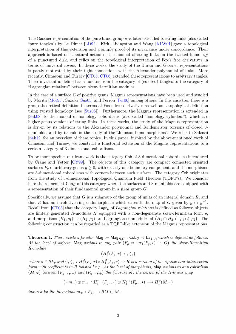
and which will be referred to as the ϕ-twisted intersection form of Fg. The following lemma,which gives a matrix presentation of 〈·, ·〉s, is obtained by straightforward computations.

Figure 3.1. The system of meridians and parallels (α, β) on the surface Fg.

Lemma 3.1. Let (α, β) := (α1, . . . , αg, β1, . . . , βg) be a “system of meridians and parallels” inthe oriented surface Fg as shown in Figure 3.1, and let (aϕ, bϕ) := (aϕ1 , . . . , a

ϕg , b

ϕ1 , . . . , b

ϕg ) be the

basis of the free R-module Hϕ1 (Fg, ?) defined by the homology classes

∀i = 1, . . . , g, aϕi :=[1⊗ αi

], bϕi :=

[1⊗ βi

]. (3.9)

The matrix of 〈·, ·〉s in the basis (aϕ, bϕ) is the skew-Hermitian matrix of size 2g

Sϕ :=

(Sϕaa Sϕab

Sϕba Sϕbb

)(3.10)

where

Sϕaa :=

ϕ(α1)− ϕ(α1) −Pϕ(α1, α2) · · · · · · −Pϕ(α1, αg)

Pϕ(α2, α1) ϕ(α2)− ϕ(α2) · · · · · · −Pϕ(α2, αg)

......

. . ....

...... ϕ(αg−1)− ϕ(αg−1) −Pϕ(αg−1, αg)

Pϕ(αg , α1) Pϕ(αg , α2) · · · Pϕ(αg , αg−1) ϕ(αg)− ϕ(αg)

Sϕab :=

Qϕ(α1, β1) −Pϕ(α1, β2) · · · · · · −Pϕ(α1, βg)

Pϕ(α2, β1) Qϕ(α2, β2) · · · · · · −Pϕ(α2, βg)

......

. . ....

...... Qϕ(αg−1, βg−1) −Pϕ(αg−1, βg)

Pϕ(αg , β1) Pϕ(αg , β2) · · · Pϕ(αg , βg−1) Qϕ(αg , βg)

= −

(Sϕba)t

13

Sϕbb :=

ϕ(β1)− ϕ(β1) −Pϕ(β1, β2) · · · · · · −Pϕ(β1, βg)

Pϕ(β2, β1) ϕ(β2)− ϕ(β2) · · · · · · −Pϕ(β2, βg)

......

. . ....

...... ϕ(βg−1)− ϕ(βg−1) −Pϕ(βg−1, βg)

Pϕ(βg , β1) Pϕ(βg , β2) · · · Pϕ(βg , βg−1) ϕ(βg)− ϕ(βg)

with Pϕ(x, y) := (1−ϕ(x))(1−ϕ(y)), Qϕ(x, y) := (ϕ(x)+1)(ϕ(y)+1)−2 for any x, y ∈ H1(Fg).

It can be verified that the determinant of the matrix Sϕ given by Lemma 3.1 is 4g: therefore theform 〈·, ·〉s is non-degenerate. Moreover, (3.5) shows that

∀x ∈ Hϕ1 (Fg, ?), 〈x, ν〉s = 2 ∂∗(x). (3.11)

(Here, by a slight abuse of notation, we simply denote by ν ∈ Hϕ1 (Fg, ?) the homology class

[1⊗ ν], where ν ⊂ Fg is the lift of the oriented curve ν to the maximal abelian cover that startsat the preferred lift ? of the base-point ?.) Let Q(R) be the field of fractions of R and set

ν/2 := (1/2)⊗ ν ∈ Q(R)⊗R Hϕ1 (Fg, ?).

It follows from (3.11) that the triple(Hϕ

1 (Fg, ?), 〈·, ·〉s, ν/2)is a pointed skew-Hermitian R-

module in the sense of Section 2.4.

3.3 The equivariant intersection form S

We now recall a few facts about Reidemeister’s equivariant intersection forms [Rei39]. Let N bea piecewise-linear compact connected oriented n-manifold, and let J, J ′ be two disjoint subsetsof ∂N . (We possibly have J = ∅ or J ′ = ∅, or even ∂N = ∅.) We assume that N is endowedwith a triangulation T , such that J is a subcomplex of T and J ′ is a subcomplex of the dualcellular decomposition T ∗.

Fix a ring R and a multiplicative subgroup G ⊂ R× as in (3.6), and let ϕ : H1(N) → G be agroup homomorphism. The equivariant intersection form of N (with coefficients in R twisted byϕ, relative to J t J ′) is the sesquilinear map

SN := SN,ϕ,JtJ ′ : Hϕq (N, J)×Hϕ

n−q(N, J′) −→ R

defined for any q ∈ {0, . . . , n} by

SN

([∑

i

ri ⊗ xi],[∑

i′

r′i′ ⊗ x′i′])

:=∑

i,i′

∑

h∈H1(N)

(hxi • x′i′)ϕ(h−1) ri r′i′

where∑

i ri ⊗ xi ∈ Cϕq (T, J) and

∑i′ r′i′ ⊗ x′i′ ∈ C

ϕn−q(T

∗, J ′) are arbitrary cellular cycles. Hereri, r

′i′ are elements of R, xi ⊂ N is a lift of an oriented q-simplex of T not included in J , hxi

is the image of xi under the deck transformation of N corresponding to h ∈ H1(N), x′i′ ⊂ N isa lift of an oriented (n − q)-cell of T ∗ not included in J ′, and (hxi • x′i′) ∈ {−1, 0,+1} denotesthe intersection number. We recall Blanchfield’s duality theorem in the following form, which isadapted to our setting and can be easily deduced from [Bla57, Theorem 2.6].

Theorem 3.2 (Blanchfield). The left and right annihilators of SN are the torsion submodulesof Hϕ

q (N, J) and Hϕn−q(N, J

′), respectively.

14

Assume now that N := Fg. Let l, r ∈ ∂Fg be some points such that l < ? < r if we follow∂Fg in the positive direction. Then the arc joining l to ? in ∂Fg \ {r} induces an isomorphismHϕ

1 (Fg, ?)'Hϕ1 (Fg, l) and, similarly, the arc joining ? to r in ∂Fg \ {l} induces an isomorphism

Hϕ1 (Fg, ?)'Hϕ

1 (Fg, r). It is easily deduced from the definitions that the diagram

Hϕ1 (Fg, l)×Hϕ

1 (Fg, r)S // R

Hϕ1 (Fg, ?)×Hϕ

1 (Fg, ?) 〈·,·〉//

'OO

R

(3.12)

is commutative, where we denote S := SFg ,ϕ,{l}t{r} and 〈·, ·〉 is the pairing defined by (3.7).Since the form S is non-degenerate by Theorem 3.2, we recover from (3.8) and (3.11) the factthat 〈·, ·〉s is non-degenerate.

4 The Magnus functor

In this section, we construct the Magnus functor and prove some of its properties. We fix aring R and a multiplicative subgroup G ⊂ R× as in (3.6).

4.1 The functor Mag

Here is the main result of this section.

Theorem 4.1. There is a functor Mag := MagR,G : CobG → pLagrR defined by

Mag(g, ϕ) :=(Hϕ

1 (Fg, ?), 〈·, ·〉s, ν/2)

for any object (g, ϕ) of CobG, and by

Mag(M,ϕ) := cl(

ker((−m−)⊕m+ : H

ϕ−1 (Fg− , ?)⊕H

ϕ+

1 (Fg+ , ?)→ Hϕ1 (M, ?)

))

for any morphism (M,ϕ) : (g−, ϕ−)→ (g+, ϕ+) in CobG.

This is an analogue of [CT05, Theorem 3.5] and [CT05, Theorem 6.1] for cobordisms. The proofis done in the next subsection.

4.2 Proof of Theorem 4.1

We will use the same strategy of proof as in [CT05, Section 4]. It suffices to prove the followingtwo lemmas.

Lemma 4.2. Let (M,ϕ) ∈ CobG((g−, ϕ−), (g+, ϕ+)). Then the closure of

ker((−m−)⊕m+ : H

ϕ−1 (Fg− , ?)⊕H

ϕ+

1 (Fg+ , ?) −→ Hϕ1 (M, ?)

)

is a Lagrangian submodule of Hϕ−1 (Fg− , ?) ⊕ H

ϕ+

1 (Fg+ , ?). Furthermore, it contains (ν−, ν+)where ν± := [1⊗ ν] denotes the “boundary” element of Hϕ±

1 (Fg± , ?).

15

Lemma 4.3. Let (M,ϕ) ∈ CobG((g−, ϕ−), (g+, ϕ+)) and (N,ψ) ∈ CobG((h−, ψ−), (h+, ψ+)) besuch that (g+, ϕ+) = (h−, ψ−). Then Mag(N ◦M,ψ + ϕ) = Mag(N,ψ) ◦Mag(M,ϕ).

Let (M,ϕ) ∈ CobG((g−, ϕ−), (g+, ϕ+)). Observe that the “vertical” boundary m(S1 × [−1, 1])of the cobordism M can be collapsed onto the circle m(S1 × {0}) without changing the home-omorphism type of M . Thus we can assume that m+(∂Fg+) = m−(∂Fg−) ⊂ ∂M , so that the“bottom boundary” ∂−M = m−(Fg−) and the “top boundary” ∂+M = m+(Fg+) share the samebase point ? ∈ ∂M . Let

µ : Hϕ−1 (Fg− , ?)⊕H

ϕ+

1 (Fg+ , ?) −→ Hϕ1 (∂M, ?) (4.1)

be the direct sum of the opposite of the homomorphism induced by m− : Fg− → ∂M with thehomomorphism induced by m+ : Fg+ → ∂M . The long exact sequence for the pair (∂M, ?)shows that Hϕ

1 (∂M) can be regarded as a submodule of Hϕ1 (∂M, ?). The following lemma is

needed for the proof of Lemma 4.2.

Lemma 4.4. If a, b ∈ Hϕ−1 (Fg− , ?)⊕H

ϕ+

1 (Fg+ , ?) are such that µ(a), µ(b) ∈ Hϕ1 (∂M), then

〈a, b〉s = 2S∂M(µ(a), µ(b)

)

where 〈·, ·〉s denotes the skew-Hermitian form (−〈·, ·〉s) ⊕ 〈·, ·〉s on Hϕ−1 (Fg− , ?) ⊕ H

ϕ+

1 (Fg+ , ?),and S∂M : Hϕ

1 (∂M)×Hϕ1 (∂M)→ R is the equivariant intersection form of ∂M .

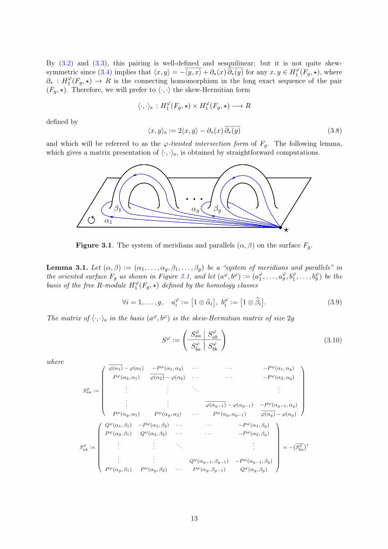
Proof. We first describe how the maximal abelian cover ∂M of ∂M can be constructed from themaximal abelian covers Fg− and Fg+ of Fg− and Fg+ , respectively. Consider a copy y · Fg− ofFg− for every y ∈ H1(Fg+) and, similarly, consider a copy x·Fg+ of Fg+ for every x ∈ H1(Fg−).In the sequel, the abelian group H1(Fg±) is denoted multiplicatively. The copy 1· Fg± indexedby the identity element 1 ∈ H1(Fg∓) is simply denoted by Fg± , and its preferred based point issimply denoted by ?. Let ν± ⊂ Fg± be the unique lift of the circle ν± := ∂Fg± that containsthe base-point ?: the preimage of ν± in Fg± consists of all the circles z · ν± obtained from ν±

by the deck transformations z ∈ H1(Fg±). Then ∂M is the connected surface obtained from thedisjoint union ( ⊔

y∈H1(Fg+ )

y ·Fg−)t( ⊔

x∈H1(Fg− )

x·Fg+)

by connecting with a tube the circle y·(x·ν−) in the copy y·Fg− to the circle x·(y·ν+) in the copyx ·Fg+ , for any x ∈ H1(Fg−) and y ∈ H1(Fg+). The action of H1(∂M) ' H1(Fg−) ⊕ H1(Fg+)

by deck transformations on ∂M is the obvious action that is suggested by our notations: seeFigure 4.1.

Let l, r ∈ ∂Fg± be some points such that l < ? < r if we follow ∂Fg± in the positive direction.Let ν?l be the oriented arc joining ? to l in ∂Fg± \ {r}, and let ν?r be the oriented arc joining? to r in ∂Fg± \ {l}: the endpoints of the lifts of ν?l and ν?r to Fg± that start at ? are denotedby l and r respectively. Consider now some elements r−,k, r+,k ∈ R (where k ranges over a finiteset) and some loops α−,k in Fg− and α+,k in Fg+ based at l, such that

∑

k

r−,k(ϕ−([α−,k])− 1

)=∑

k

r+,k

(ϕ+([α+,k])− 1

)∈ R. (4.2)

16

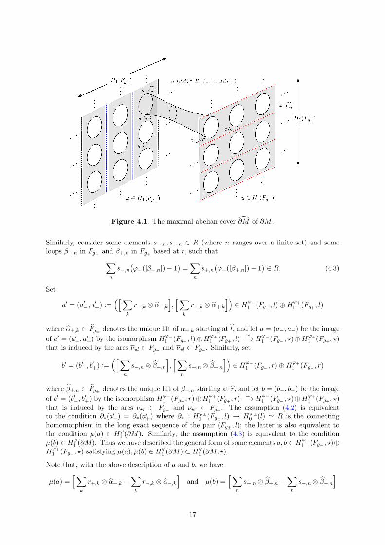
Figure 4.1. The maximal abelian cover ∂M of ∂M .

Similarly, consider some elements s−,n, s+,n ∈ R (where n ranges over a finite set) and someloops β−,n in Fg− and β+,n in Fg+ based at r, such that

∑

n

s−,n(ϕ−([β−,n])− 1

)=∑

n

s+,n

(ϕ+([β+,n])− 1

)∈ R. (4.3)

Set

a′ = (a′−, a′+) :=

([∑

k

r−,k ⊗ α−,k],[∑

k

r+,k ⊗ α+,k

])∈ Hϕ−

1 (Fg− , l)⊕Hϕ+

1 (Fg+ , l)

where α±,k ⊂ Fg± denotes the unique lift of α±,k starting at l, and let a = (a−, a+) be the imageof a′ = (a′−, a

′+) by the isomorphism H

ϕ−1 (Fg− , l)⊕H

ϕ+

1 (Fg+ , l)'−→ H

ϕ−1 (Fg− , ?)⊕H

ϕ+

1 (Fg+ , ?)that is induced by the arcs ν?l ⊂ Fg− and ν?l ⊂ Fg+ . Similarly, set

b′ = (b′−, b′+) :=

([∑

n

s−,n ⊗ β−,n],[∑

n

s+,n ⊗ β+,n

])∈ Hϕ−

1 (Fg− , r)⊕Hϕ+

1 (Fg+ , r)

where β±,n ⊂ Fg± denotes the unique lift of β±,n starting at r, and let b = (b−, b+) be the imageof b′ = (b′−, b

′+) by the isomorphism H

ϕ−1 (Fg− , r)⊕H

ϕ+

1 (Fg+ , r)'−→ H

ϕ−1 (Fg− , ?)⊕H

ϕ+

1 (Fg+ , ?)that is induced by the arcs ν?r ⊂ Fg− and ν?r ⊂ Fg+ . The assumption (4.2) is equivalentto the condition ∂∗(a

′−) = ∂∗(a

′+) where ∂∗ : H

ϕ±1 (Fg± , l) → H

ϕ±0 (l) ' R is the connecting

homomorphism in the long exact sequence of the pair (Fg± , l); the latter is also equivalent tothe condition µ(a) ∈ Hϕ

1 (∂M). Similarly, the assumption (4.3) is equivalent to the conditionµ(b) ∈ Hϕ

1 (∂M). Thus we have described the general form of some elements a, b ∈ Hϕ−1 (Fg− , ?)⊕

Hϕ+

1 (Fg+ , ?) satisfying µ(a), µ(b) ∈ Hϕ1 (∂M) ⊂ Hϕ

1 (∂M, ?).

Note that, with the above description of a and b, we have

µ(a) =[∑

k

r+,k ⊗ α+,k −∑

k

r−,k ⊗ α−,k]

and µ(b) =[∑

n

s+,n ⊗ β+,n −∑

n

s−,n ⊗ β−,n]

17

where α±,k and β±,n are now regarded as 1-chains in ∂M thanks to the inclusion Fg± ⊂ ∂M .(It follows from (4.2) and (4.3) that the above 1-chains are indeed 1-cycles in Cϕ(∂M) =

R⊗Z[H1(∂M)] C(∂M).) We deduce that

S∂M (µ(a), µ(b)) = S(Fg+ )

([∑

k

r+,k ⊗ α+,k

],[∑

n

s+,n ⊗ β+,n

])

+S(−Fg− )

([∑

k

r−,k ⊗ α−,k],[∑

n

s−,n ⊗ β−,n])

= S(Fg+ )

(a′+, b

′+

)− S(Fg− )

(a′−, b

′−) (3.12)

= 〈a+, b+〉 − 〈a−, b−〉

where S(Fg± ) := SFg± ,ϕ±,{l}t{r} is the equivariant intersection form of Fg± . Furthermore, wehave ∂∗(a+) = ∂∗(a−) and ∂∗(b+) = ∂∗(b−) by (4.2) and (4.3), respectively. We conclude that

2S∂M (µ(a), µ(b)) = 2〈a+, b+〉 − 2〈a−, b−〉(3.8)= 〈a+, b+〉s + ∂∗(a+)∂∗(b+)− 〈a−, b−〉s − ∂∗(a−)∂∗(b−)

= 〈a+, b+〉s − 〈a−, b−〉s = 〈a, b〉s.

The rest of this subsection is devoted to the proofs of Lemma 4.2 and Lemma 4.3.

Proof of Lemma 4.2. The arguments below follow the same lines as [CT05, Lemma 3.3], but thereare also some technical complications due to the peculiarities of the twisted intersection form〈·, ·〉s. We start with a preliminary observation. Denote by j : ∂M →M and by j? : (∂M, ?)→(M,?) the inclusions, and consider the following commutative diagram:

0 Hϕ1 (∂M) Hϕ

1 (∂M, ?) ∂∗(Hϕ

1 (∂M, ?))

0

0 Hϕ1 (M) Hϕ

1 (M, ?) ∂∗(Hϕ

1 (M,?))

0

∂∗

∂∗

j j?

Here the rows are extracted from the long exact sequences of the pairs (∂M, ?) and (M, ?),∂∗(Hϕ

1 (∂M, ?))is the submodule of Hϕ

0 (?) ' R generated by the ϕj(h)− 1 for all h ∈ H1(∂M),∂∗(Hϕ

1 (M,?))is the submodule generated by the ϕ(h) − 1 for all h ∈ H1(M), and the map

∂∗(Hϕ

1 (∂M, ?))→ ∂∗

(Hϕ

1 (M,?))is the inclusion. It follows from the “ker-coker” lemma that

ker j = ker j?: in other words, if we continue to regard Hϕ1 (∂M) as a submodule of Hϕ

1 (∂M, ?),then our observation is that K := ker j? is contained in Hϕ

1 (∂M).

The above being taken into account, we now have to prove that the closure cl(L) of

L := ker(

(−m−)⊕m+ : Hϕ−1 (Fg− , ?)⊕H

ϕ+

1 (Fg+ , ?) −→ Hϕ1 (M, ?)

)

in Hϕ−1 (Fg− , ?)⊕H

ϕ+

1 (Fg+ , ?) is a Lagrangian submodule. We first claim the following:

(i) The annihilator Ann(K) of K with respect to S∂M : Hϕ1 (∂M)×Hϕ

1 (∂M) → R coincideswith the closure cl(K) of K in Hϕ

1 (∂M).

(ii) We have µ(L) = K where µ is the homomorphism (4.1); in particular, µ(L) ⊂ Hϕ1 (∂M).

18

To prove claim (i), we consider the equivariant intersection form of M

SM := SM,ϕ,∅t∂M : Hϕ1 (M)×Hϕ

2 (M,∂M) −→ R,

which is related to the form S∂M through the following identity:

∀x ∈ Hϕ1 (∂M), ∀y ∈ Hϕ

2 (M,∂M), S∂M (x, ∂∗(y)) = ε SM (j(x), y);

here ε is a constant sign which we do not need to specify. It follows that

Ann(K) = {x ∈ Hϕ1 (∂M) : S∂M (x, ker j) = 0}

= {x ∈ Hϕ1 (∂M) : S∂M (x, ∂∗H

ϕ2 (M,∂M)) = 0}

= {x ∈ H1(∂M) : SM (j(x), Hϕ2 (M,∂M)) = 0} = j−1

(TorsR Hϕ

1 (M))

= cl(K),

where the penultimate identity follows from Blanchfield’s duality theorem (see Theorem 3.2).

We now prove claim (ii). The inclusion µ(L) ⊂ K follows immediately from the facts thatL = ker(j? ◦ µ) and K = ker j?. The converse inclusion follows by the same argument from thesurjectivity of the map µ. (This surjectivity is a consequence of the Mayer–Vietoris theorem andthe fact that Hϕ

0 (ν, ?) = 0 where ν denotes the circle m+(Fg+) ∩m−(Fg−) in ∂M .)

To proceed, we observe that the closure cl(K) of K in Hϕ1 (∂M) coincides with the closure of K

in Hϕ1 (∂M, ?), since Hϕ

1 (∂M) is the kernel of ∂∗ : Hϕ1 (∂M, ?)→ Hϕ

0 (?) ' R and R has no zero-divisor. Using (ii), it follows that cl(L) ⊂ µ−1(cl(K)) and, in particular, µ(cl(L)) is containedin Hϕ

1 (∂M). The converse inclusion µ−1(cl(K)) ⊂ cl(L) is also true: for any a ∈ µ−1(cl(K)), wehave rµ(a) ∈ K for some r ∈ R \ {0}; hence 0 = j?(rµ(a)) = (j? ◦ µ)(ra), which implies thatra ∈ L so that a ∈ cl(L). Thus, we obtain

cl(L) = µ−1(cl(K))(i)= µ−1(Ann(K))

(ii)= µ−1(Ann(µ(L))) (4.4)

where Ann(µ(L)) denotes the annihilator of µ(L) with respect to S∂M .

We can now prove that cl(L) ⊂ Ann(cl(L)). Since R has no zero-divisors, we have Ann(cl(L)) =Ann(L) so that it is enough to prove that cl(L) ⊂ Ann(L). Let a ∈ cl(L): using Lemma 4.4, weobtain

∀b ∈ L, 〈a, b〉s = 2S∂M (µ(a), µ(b))(4.4)= 0

which shows that a ∈ Ann(L) as desired.

To conclude that cl(L) is Lagrangian, it remains to show that Ann(L) ⊂ cl(L). Consider anyelement a ∈ Ann(L) ∩ µ−1(Hϕ

1 (∂M)): using Lemma 4.4, we obtain

∀b ∈ L, 2S∂M (µ(a), µ(b)) = 〈a, b〉s = 0

and it follows that µ(a) ∈ Ann(µ(L)); we deduce from (4.4) that a ∈ cl(L). Therefore weare reduced to proving that µ(Ann(L)) ⊂ Hϕ

1 (∂M). Since ker(µ) ⊂ L, we have Ann(L) ⊂Ann(ker(µ)) and it is enough to show that

µ(

Ann(ker(µ)))⊂ Hϕ

1 (∂M). (4.5)

Let a = (a−, a+) ∈ Hϕ−1 (Fg− , ?)⊕H

ϕ+

1 (Fg+ , ?) be an arbitrary element of Ann(ker(µ)). Considerthe distinguished element (ν−, ν+) ∈ Hϕ−

1 (Fg− , ?)⊕Hϕ+

1 (Fg+ , ?) defined by ν± := [1⊗ν]. Clearlyµ(ν−, ν+) = 0 (so that, in particular, (ν−, ν+) belongs to L). Therefore

0 = 〈a, (ν−, ν+)〉s = 〈a+, ν+〉s − 〈a−, ν−〉s(3.11)

= 2 ∂∗(a+)− 2 ∂∗(a−)

which implies that µ(a) ∈ Hϕ1 (∂M). This proves (4.5) and concludes the proof of the lemma.

19

Proof of Lemma 4.3. The arguments below follow very closely those of [CT05, Lemma 3.4]. Con-sider the composition of two morphisms in the category CobG

(g−, ϕ−)(M,ϕ)−→ (g+, ϕ+) = (h−, ψ−)

(N,ψ)−→ (h+, ψ+)

and recall that, after collapsing the vertical boundary ofM onto the “middle” circle m(S1×{0}),we can assume that m−(Fg−) and m+(Fg+) share the same base point ? ∈ ∂M . The sameconsideration holds for n−(Fh−) and n+(Fh+) in ∂N . Thus we have only one base point ? inwhat follows. Recall now the homomorphisms

M := (−m−)⊕m+ : Hϕ−1 (Fg− , ?)⊕H

ϕ+

1 (Fg+ , ?) −→ Hϕ1 (M, ?),

N := (−n−)⊕ n+ : Hψ−1 (Fh− , ?)⊕H

ψ+

1 (Fh+ , ?) −→ Hψ1 (N, ?),

R := (−m−)⊕ n+ : Hϕ−1 (Fg− , ?)⊕H

ψ+

1 (Fh+ , ?) −→ Hψ+ϕ1 (N ◦M, ?)

used in the definition of the Lagrangian submodules Mag(M,ϕ), Mag(N,ψ), Mag(N ◦M,ψ+ϕ)respectively. It is sufficient to prove that

ker(R) = ker(N) ◦ ker(M), (4.6)

where we use the notation (2.1). Indeed this claim implies that

Mag(N ◦M,ψ + ϕ) = cl(

ker(R))

= cl(

ker(N) ◦ ker(M))

= cl(

cl(

ker(N))◦ cl(

ker(M)))

= cl(Mag(N,ψ) ◦ Mag(M,ϕ)

)= Mag(N,ψ) ◦Mag(M,ϕ)

where the third equality holds by [CT05, Lemma 2.6].

The construction of N ◦M by identifying ∂+M and ∂−N using the boundary-parametrizationsleads to the following Mayer–Vietoris exact sequence of R-modules:

Hϕ+

1 (Fg+ , ?)ι−→ Hϕ

1 (M,?)⊕Hψ1 (N, ?)

$−→ Hψ+ϕ1 (N ◦M,?) −→ 0

Here ι := (m+,−n−) and $ is the sum of the homomorphisms induced by the inclusions of Mand N in N ◦M . Consider the commutative diagram

0 Hϕ+g+ H

ϕ−g− ⊕H

ϕ+g+ ⊕H

ψ+

h+Hϕ−g− ⊕H

ψ+

h+0

0 ker($) Hϕ1 (M,?)⊕Hψ

1 (N, ?) Hψ+ϕ1 (N ◦M,?) 0

i p

$

ι γ R

where the symbol Hρn denotes a twisted homology group Hρ

1 (Fn, ?), the homomorphism i isthe natural inclusion, p is the natural projection and the map γ is defined by γ(x, x′, x′′) :=(M(x, x′),N(x′, x′′)). On the one hand, we have

p(

ker(γ))

={

(x, x′′) ∈ Hϕ−g− ⊕H

ψ+

h+: M(x, x′) = 0 and N(x′, x′′) = 0 for some x′ ∈ Hϕ+

g+

}

= ker(N)◦ ker(M).

On the other hand, the “ker-coker” lemma applied to the above diagram shows that p(ker(γ)) =ker(R) since ι is surjective. This proves the claim (4.6).

20

4.3 Properties of the functor Mag

We show two fundamental properties of the Magnus functor. The first one involves the followingrelation among cobordisms. Two cobordisms (M1, ϕ1), (M2, ϕ2) ∈ CobG((g−, ϕ−), (g+, ϕ+)) arehomology concordant if there exists a compact connected oriented 4-manifold W with

∂W = M1 ∪m1◦m−12

(−M2)

such that the inclusion maps i1 : M1 ↪→ W and i2 : M2 ↪→ W induce isomorphisms at thelevel of H(·;Z) and satisfy ϕ1 ◦ (i1)−1 = ϕ2 ◦ (i2)−1 : H1(W ) → G. In such a situation, wewrite (M1, ϕ1) ∼H (M2, ϕ2). It is easily verified that ∼H is an equivalence relation on the setCobG((g−, ϕ−), (g+, ϕ+)) for any objects (g−, ϕ−), (g+, ϕ+), and that ∼H defines a congruencerelation on the category CobG. Besides, the monoidal structure of CobG induces a strict monoidalstructure on the quotient category CobG/∼H .

In addition to the hypothesis (3.6) on the ring R and the multiplicative subgroup G ⊂ R×,consider the following condition:

R is equipped with a ring homomorphism εR : R→ Z such that εR(G) = {1}. (4.7)

Proposition 4.5. Under the assumption (4.7), the functor Mag : CobG → pLagrR descends tothe quotient CobG/∼H .

Proof. Let (M1, ϕ1), (M2, ϕ2) ∈ CobG((g−, ϕ−), (g+, ϕ+)) be such that (M1, ϕ1) ∼H (M2, ϕ2).Let j ∈ {1, 2}. By Lemma 4.6 below, the fact that the map ij : Mj ↪→W induces an isomorphismin ordinary homology implies that

ij : Q(R)⊗R Hϕj1 (Mj , ?) ' H

ϕj,Q1 (Mj , ?) −→ H

ϕQ1 (W, ?) ' Q(R)⊗R Hχ

1 (W, ?)

is an isomorphism where χ := ϕ1i−11 = ϕ2i

−12 . Thus we get the following commutative diagram:

Q(R)⊗R Hϕ11 (M1, ?)

i1' ,,

Q(R)⊗R Hϕ±1 (Fg± , ?)

m1,± 22

m2,± ,,

Q(R)⊗R Hχ1 (W, ?)

Q(R)⊗R Hϕ21 (M2, ?)

i2

' 22

It follows from this diagram that

ker((−m1,−)⊕m1,+

)⊂((−m2,−)⊕m2,+

)−1(TorsRH

ϕ21 (M2, ?))

and ker((−m2,−)⊕m2,+

)⊂((−m1,−)⊕m1,+

)−1(TorsRH

ϕ11 (M1, ?)),

which immediately implies that

ker((−m1,−)⊕m1,+

)⊂ cl

(ker((−m2,−)⊕m2,+

))

and ker((−m2,−)⊕m2,+

)⊂ cl

(ker((−m1,−)⊕m1,+

)).

We conclude that Mag(M1, ϕ1) = Mag(M2, ϕ2).

Lemma 4.6. Assume (4.7). Let (X,Y ) be a pair of CW-complexes such that the inclusion mapi : Y → X induces an isomorphism at the level of H(· ;Z). For any group homomorphismϕ : H1(X)→ G, we have HϕQ(X,Y ) = 0 where ϕQ : Z[H1(X)]→ Q(R) is the ring homomor-phism induced by ϕ.

21

Proof. We closely follow the arguments of [KLW01, Proposition 2.1]. Since the cell chain complexC(X,Y ) with coefficients in Z is acyclic and free, we can find a chain contraction δ : C(X,Y )→C(X,Y ), i.e. a degree 1 map of graded Z-modules satisfying δ∂+∂δ = Id. Let pX : X → X be themaximal abelian cover of X and choose, for every relative cell of (X,Y ), an orientation and a liftto X. We also order the relative cells of (X,Y ) in an arbitrary way. All those choices define a Z-basis of C(X,Y ) and a Z[H1(X)]-basis of C(X, p−1

X (Y )), and there is a one-to-one correspondencebetween these two basis: thus we can identify C(X, p−1

X (Y )) with Z[H1(X)]⊗Z C(X,Y ). So, δextends to a Z[H1(X)]-linear map δ : C(X, p−1

X (Y ))→ C(X, p−1X (Y )) of degree 1. The map

N := Q(R)⊗Z[H1(X)]

(δ∂ + ∂δ

): CϕQ(X,Y ) −→ CϕQ(X,Y )

is clearly a chain map, which induces the null map at the level of homology. On the other hand,we have

εR det(R⊗Z[H1(X)] (δ∂ + ∂δ)

)= εR ϕdet

(δ∂ + ∂δ

)= εdet

(δ∂ + ∂δ

)= 1

where ε : Z[H1(X)] → Z denotes the augmentation of the group ring Z[H1(X)]. The aboveidentity implies that det(N) 6= 0. We conclude that N is an isomorphism of chain complexesand that CϕQ(X,Y ) is acyclic.

The second property of the Magnus functor to be shown is the monoidality.

Proposition 4.7. Mag : CobG → pLagrR is a strong monoidal functor.

Proof. Recall that CobG and pLagrR are viewed as strict monoidal categories (see Remark 2.4).We first define a natural transformation T between the functors Mag(·)�Mag(·) and Mag(·� ·).For any object (k, κ) of the category CobG, we denote Mag(k, κ) =

(Hκ

1 (Fk, ?), 〈·, ·〉(k)s , ν(k)/2

).

Thus, for any objects (g, ϕ) and (h, ψ) of the category CobG, we have

Mag(g, ϕ) �Mag(h, ψ) =(Hϕ

1 (Fg, ?)⊕Hψ1 (Fh, ?) , 〈·, ·〉(g)s ν(g)/2⊕ν(h)/2 〈·, ·〉

(h)s , ν(g)/2 + ν(h)/2

)

andMag

((g, ϕ) � (h, ψ)

)=(Hϕ⊕ψ

1 (Fg+h, ?), 〈·, ·〉(g+h)s , ν(g+h)/2

).

We claim that the R-linear map Hϕ1 (Fg, ?)⊕Hψ

1 (Fh, ?)→ Hϕ⊕ψ1 (Fg+h, ?) induced by the inclu-

sions of Fg and Fh in Fg]∂Fh = Fg+h defines an isomorphism

T(g,ϕ),(h,ψ) : Mag(g, ϕ) �Mag(h, ψ) −→ Mag((g, ϕ) � (h, ψ)

)

in the category pUR. Clearly, T(g,ϕ),(h,ψ) maps ν(g)/2 + ν(h)/2 to ν(g+h)/2 since the boundarycurve of Fg]∂Fh is the connected sum of the boundary curves of Fg and Fh. Thus the claimreduces to proving that T(g,ϕ),(h,ψ) is unitary. Let x, y ∈ Hϕ

1 (Fg, ?) and z, t ∈ Hψ1 (Fh, ?), and

denote by x′, y′, z′, t′ their images in Hϕ⊕ψ1 (Fg+h, ?): we have

(〈·, ·〉(g)s ν(g)/2⊕ν(h)/2〈·, ·〉

(h)s

)(x+ z, y + t)

= 〈x, y〉(g)s + 〈z, t〉(h)s + 〈x, ν(g)/2〉(g)s 〈ν(h)/2, t〉(h)

s − 〈ν(g)/2, y〉(g)s 〈z, ν(h)/2〉(h)s

(3.11)= 〈x, y〉(g)s + 〈z, t〉(h)

s − ∂∗(x) ∂∗(t) + ∂∗(y) ∂∗(z)

22

and

〈x′ + z′, y′ + t′〉(g+h)s

= 〈x, y〉(g)s + 〈z, t〉(h)s + 〈x′, t′〉(g+h)

s − 〈y′, z′〉(g+h)s

(3.8)= 〈x, y〉(g)s + 〈z, t〉(h)

s +(2〈x′, t′〉(g+h) − ∂∗(x′) ∂∗(t′)

)−(2〈y′, z′〉(g+h) − ∂∗(y′) ∂∗(z′)

)

= 〈x, y〉(g)s + 〈z, t〉(h)s − ∂∗(x)∂∗(t) + ∂∗(y)∂∗(z)

which proves our claim about T(g,ϕ),(h,ψ). By applying the “graph” functor pUR → pLagrR, weobtain an isomorphism T(g,ϕ),(h,ψ) : Mag(g, ϕ)�Mag(h, ψ)→ Mag

((g, ϕ)�(h, ψ)

)in the category

pLagr. This isomorphism is natural since, for any

(M,ϕ) ∈ CobG((g−, ϕ−), (g+, ϕ+)

)and (N,ψ) ∈ CobG

((h−, ψ−), (h+, ψ+)

),

we have

T−1(g+,ϕ+),(h+,ψ+) ◦Mag

((M,ϕ) � (N,ψ)

)◦ T(g−,ϕ−),(h−,ψ−)

= cl(ker((−m− ⊕−n−)⊕ (m+ ⊕ n+)

))

' cl(ker((−m− ⊕m+)⊕ (−n− ⊕ n+)

))

= cl(

ker(−m− ⊕m+)⊕ ker(−n− ⊕ n+))

= cl(

ker(−m− ⊕m+))⊕ cl

(ker(−n− ⊕ n+)

)= Mag(M,ϕ) �Mag(N,ψ).

Recall that the unit object of CobG is the pair I consisting of the integer 0 and the trivialgroup homomorphism H1(F0)→ G, and that the unit object of pLagrR is I := ({0}, 0, 0). Thuswe have Mag(I) = (H1(F0, ?), 0, 0) = I, and we define U : I → Mag(I) to be the identity.It is immediately checked that the morphism U and the natural transformation T satisfy thecoherence conditions that make Mag into a strong monoidal functor.

Remark 4.8. Proposition 4.5 is the analogue of the invariance under concordance of tangles whichCimasoni and Turaev mentioned for their functor [CT05, end of §3.3]. The tangle analogue ofProposition 4.7 does not seem to have been addressed in [CT05].

5 Examples and computations

We give examples and explain how to compute the Magnus functor using Heegaard splittings.

5.1 The Magnus representation

Fix an integer g ≥ 1. A homology cobordism over Fg is a morphism M ∈ Cob(g, g) such thatm± : H1(Fg)→ H1(M) are isomorphisms. The set of equivalence classes of homology cobordismsdefines a submonoid C(Fg) ⊂ Cob(g, g).

Let G be an abelian group and fix a group homomorphism ϕ : H1(Fg)→ G. Here we will onlyconsider those M ∈ C(Fg) such that the composition

H1(Fg)m−−→'H1(M)

m−1+−→'H1(Fg)

ϕ−→ G

23

coincides with ϕ. By equipping any such cobordism M with the group homomorphism ϕ :=ϕm−1

+ = ϕm−1− , we define a submonoid Cϕ(Fg) ⊂ CobG

((g, ϕ), (g, ϕ)

).

Assume now that G is a multiplicative subgroup of a commutative ring R, satisfying (3.6)and (4.7). Let Q := Q(R) be the field of fractions of R, and denote by ϕQ : Z[H1(Fg)] → Qthe ring homomorphism induced by ϕ : H1(Fg) → G. For any M ∈ Cϕ(Fg), the fact thatm± : H1(Fg) → H1(M) is an isomorphism of abelian groups implies that m± : H

ϕQ1 (Fg, ?) →

HϕQ1 (M,?) is an isomorphism ofQ-vector spaces (see Lemma 4.6). Thus, rϕ(M) := (m+)−1 ◦ m−

is an automorphism ofHϕQ1 (Fg, ?). TheMagnus representation is the monoid homomorphism

rϕ : Cϕ(Fg) −→ AutQ(HϕQ1 (Fg, ?)

).

The reader is referred to [Sak12] for a survey of this invariant of homology cobordisms.

We now describe the group of units of the monoid Cϕ(Fg). Let MCG(Fg) be the mapping classgroup of the surface Fg, which consists of the isotopy classes of self-homeomorphisms of Fg fixing∂Fg pointwise. Themapping cylinder construction, which associates to any such homeomorphismf the cobordism

c(f) :=(Fg × [−1, 1], (f × {−1}) ∪ (∂Fg × Id) ∪ (Id×{1})

)

defines a monoid homomorphism c : MCG(Fg) → C(Fg). It is well-known that c is injectiveand that its image is the group of units of C(Fg): see [HM12, §2.2], for instance. Thus thesubgroup

MCGϕ(Fg) :={f ∈ MCG(Fg) : ϕf = ϕ ∈ Hom(H1(Fg), G)

}

of the mapping class group is mapped by c isomorphically onto the group of units of Cϕ(Fg).Classically, the Magnus representation refers to the group homomorphism

rϕ : MCGϕ(Fg) −→ AutR(Hϕ

1 (Fg, ?))

which maps any f ∈ MCGϕ(Fg) to the isomorphism of R-modules f : Hϕ1 (Fg, ?) → Hϕ

1 (Fg, ?).Thus we have the following commutative diagram:

Cϕ(Fg) AutQ(H

ϕQ

1 (Fg, ?))

MCGϕ(Fg) AutR(Hϕ

1 (Fg, ?))

rϕ

c

rϕ

IdQ ⊗R(·)

The next proposition says that the restriction of the functor Mag := MagR,G to the submonoidCϕ(Fg) of homology cobordisms is equivalent to the Magnus representation rϕ.

Proposition 5.1. Let g ≥ 1 be an integer and let ϕ : H1(Fg) → G be a group homomorphism.Under the assumptions (3.6) and (4.7) on R and G, we have the commutative diagram

CobG((g, ϕ), (g, ϕ)

)pLagrR

(Mag(g, ϕ),Mag(g, ϕ)

)

Cϕ(Fg) pUrQ

(Mag(g, ϕ),Mag(g, ϕ)

)

Mag

rϕ

where Mag(g, ϕ) is the pointed skew-Hermitian R-module(Hϕ

1 (Fg, ?), 〈·, ·〉s, ν/2).

24

Proof. For later use, we will prove a slightly more general result. We consider some grouphomomorphisms ϕ± : H1(Fg) → G and assume that M ∈ C(Fg) is a cobordism such thatϕ− ◦m−1

− = ϕ+ ◦m−1+ : H1(M)→ G. We claim that

Mag(M,ϕ) = Γrρ (5.1)

where ϕ := ϕ± ◦m−1± and Γr

ρ is the restricted graph of the Q-linear isomorphism

ρ :=((m+)−1 ◦m− : H

ϕ−,Q1 (Fg, ?) −→ H

ϕ+,Q

1 (Fg, ?)).

The special case where ϕ− = ϕ+ implies the proposition. To prove (5.1), we consider thehomomorphisms

M := (−m−)⊕m+ : Hϕ−1 (Fg, ?)⊕Hϕ+

1 (Fg, ?) −→ Hϕ1 (M,?)

andMQ := (−m−)⊕m+ : H

ϕ−,Q1 (Fg, ?)⊕H

ϕ+,Q

1 (Fg, ?) −→ HϕQ1 (M,?).

Since the torsion submodule of Hϕ1 (M,?) is the kernel of the canonical homomorphism from

Hϕ1 (M,?) to Q⊗R Hϕ

1 (M,?) ' HϕQ1 (M,?), we have

Mag(M,ϕ) = cl(

kerM)

= M−1(

TorsRHϕ1 (M,?)

)

= (kerMQ) ∩(Hϕ−1 (Fg, ?)⊕Hϕ+

1 (Fg, ?))

= Γρ ∩(Hϕ−1 (Fg, ?)⊕Hϕ+

1 (Fg, ?))

= Γrρ.

Remark 5.2. Proposition 5.1 implies that rϕ(M) is unitary with respect to the skew-Hermitianform 〈·, ·〉s on H

ϕQ1 (Fg, ?). This is well-known: see [Sak07, Theorem 2.4] for an equivalent result.

5.2 Computations with Heegaard splittings

For any g ≥ 0, let (α1, . . . , αg, β1, . . . , βg) be the system of “meridians and parallels” in thesurface Fg shown in Figure 3.1. We denote by Cg0 ∈ Cob(0, g) the cobordism obtained fromFg × [−1, 1] by attaching g 2-handles along the curves α1 × {−1}, . . . , αg × {−1}. Similarly, letC0g ∈ Cob(g, 0) be the cobordism obtained from Fg × [−1, 1] by attaching g 2-handles along the

curves β1×{1}, . . . , βg ×{1}. Note that both C0g and Cg0 are handlebodies of genus g, which we

call upper handlebody and lower handlebody, respectively.

A Heegaard splitting of a cobordismM ∈ Cob(g−, g+) is a decomposition in the monoidal categoryCob of the form

M =(C0r+ � Idg+

)◦ c(f) ◦

(Cr−0 � Idg−

)(5.2)

where r−, r+ are some non-negative integers such that g+ +r+ = g−+r− and f ∈ MCG(Fg±+r±).Such a decomposition of M always exists: see [Ker03b, Theorem 5], for instance.

Assume now given a ring R and a multiplicative subgroup G ⊂ R× satisfying (3.6). Let (M,ϕ) ∈CobG((g−, ϕ−), (g+, ϕ+)) for which we wish to compute the Magnus functor. Any Heegaardsplitting (5.2) of M induces a decomposition

Mag(M,ϕ) =(Mag

(C0r+ , ϕ

)� IdMag(g+,ϕ+)

)◦Mag

(c(f), ϕ

)◦(Mag

(Cr−0 , ϕ

)� IdMag(g−,ϕ−)

)

(5.3)

25

in the monoidal category pLagrR where, for any submanifold S of M , the map ϕ : H1(S) → Gdenotes the group homomorphism induced by ϕ through the inclusion S ↪→ M . Recall thatthe identity of Mag(g±, ϕ±) =

(Hϕ±1 (Fg± , ?), 〈·, ·〉s, ν/2

)in pLagrR is simply the diagonal of

Hϕ±1 (Fg± , ?). Thus the computation of the functor Mag can be reduced to its evaluations on

upper handlebodies, lower handlebodies and mapping cylinders, which we determine below.

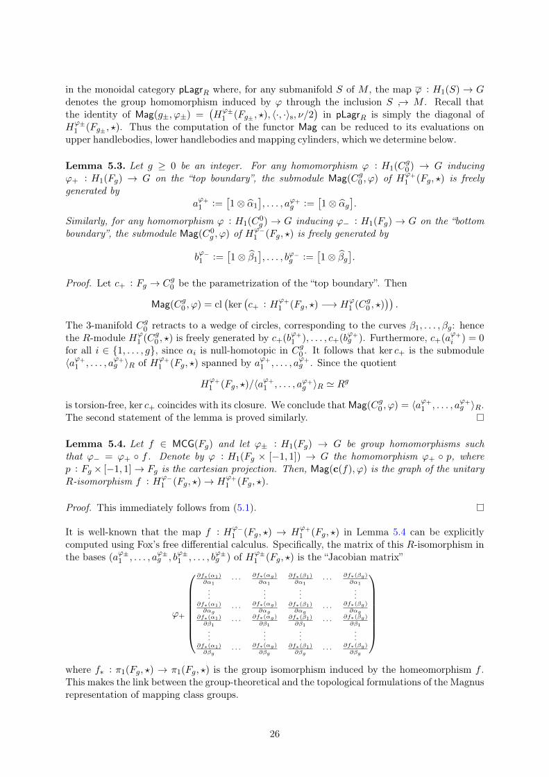
Lemma 5.3. Let g ≥ 0 be an integer. For any homomorphism ϕ : H1(Cg0 ) → G inducingϕ+ : H1(Fg) → G on the “top boundary”, the submodule Mag(Cg0 , ϕ) of Hϕ+

1 (Fg, ?) is freelygenerated by

aϕ+

1 :=[1⊗ α1

], . . . , aϕ+

g :=[1⊗ αg

].

Similarly, for any homomorphism ϕ : H1(C0g ) → G inducing ϕ− : H1(Fg) → G on the “bottom

boundary”, the submodule Mag(C0g , ϕ) of Hϕ−

1 (Fg, ?) is freely generated by

bϕ−1 :=

[1⊗ β1

], . . . , bϕ−g :=

[1⊗ βg

].

Proof. Let c+ : Fg → Cg0 be the parametrization of the “top boundary”. Then

Mag(Cg0 , ϕ) = cl(ker(c+ : H

ϕ+

1 (Fg, ?) −→ Hϕ1 (Cg0 , ?)

)).

The 3-manifold Cg0 retracts to a wedge of circles, corresponding to the curves β1, . . . , βg: hencethe R-module Hϕ

1 (Cg0 , ?) is freely generated by c+(bϕ+

1 ), . . . , c+(bϕ+g ). Furthermore, c+(a

ϕ+

i ) = 0for all i ∈ {1, . . . , g}, since αi is null-homotopic in Cg0 . It follows that ker c+ is the submodule〈aϕ+

1 , . . . , aϕ+g 〉R of Hϕ+

1 (Fg, ?) spanned by aϕ+

1 , . . . , aϕ+g . Since the quotient

Hϕ+

1 (Fg, ?)/〈aϕ+

1 , . . . , aϕ+g 〉R ' Rg

is torsion-free, ker c+ coincides with its closure. We conclude thatMag(Cg0 , ϕ) = 〈aϕ+

1 , . . . , aϕ+g 〉R.

The second statement of the lemma is proved similarly.

Lemma 5.4. Let f ∈ MCG(Fg) and let ϕ± : H1(Fg) → G be group homomorphisms suchthat ϕ− = ϕ+ ◦ f . Denote by ϕ : H1(Fg × [−1, 1]) → G the homomorphism ϕ+ ◦ p, wherep : Fg × [−1, 1]→ Fg is the cartesian projection. Then, Mag(c(f), ϕ) is the graph of the unitaryR-isomorphism f : H

ϕ−1 (Fg, ?)→ H

ϕ+

1 (Fg, ?).

Proof. This immediately follows from (5.1).

It is well-known that the map f : Hϕ−1 (Fg, ?) → H

ϕ+

1 (Fg, ?) in Lemma 5.4 can be explicitlycomputed using Fox’s free differential calculus. Specifically, the matrix of this R-isomorphism inthe bases (a

ϕ±1 , . . . , a

ϕ±g , b

ϕ±1 , . . . , b

ϕ±g ) of Hϕ±

1 (Fg, ?) is the “Jacobian matrix”

ϕ+

∂f∗(α1)∂α1

· · · ∂f∗(αg)

∂α1

∂f∗(β1)∂α1

· · · ∂f∗(βg)∂α1

......

......

∂f∗(α1)∂αg

· · · ∂f∗(αg)

∂αg

∂f∗(β1)∂αg

· · · ∂f∗(βg)∂αg

∂f∗(α1)∂β1

· · · ∂f∗(αg)

∂β1

∂f∗(β1)∂β1

· · · ∂f∗(βg)∂β1

......

......

∂f∗(α1)∂βg

· · · ∂f∗(αg)

∂βg

∂f∗(β1)∂βg

· · · ∂f∗(βg)∂βg

where f∗ : π1(Fg, ?) → π1(Fg, ?) is the group isomorphism induced by the homeomorphism f .This makes the link between the group-theoretical and the topological formulations of the Magnusrepresentation of mapping class groups.

26

5.3 The case of trivial coefficients

Consider the simplest case where G := {1}, R := Z and the involution r 7→ r of R is the identity.Then, the Magnus functor Mag := MagR,G provides a strong monoidal functor

Mag : Cob/∼H −→ LagrZ

where LagrZ denotes the category of Lagrangian relations between symplectic Z-modules. Specif-ically, the functor Mag assigns to any object g the symplectic Z-module

Mag(g) =(H1(Fg), 〈·, ·〉

), (5.4)

where H1(Fg) = H1(Fg;Z) is the ordinary homology and 〈·, ·〉 is the usual homology intersectionform, and it assigns to any morphism M ∈ Cob(g−, g+) the Lagrangian submodule

Mag(M) = cl(

ker((−m−)⊕m+ : H1(Fg−)⊕H1(Fg+) −→ H1(M)

)), (5.5)

which is a free direct summand of H1(Fg−)⊕H1(Fg+) of rank g−+g+. Note that, with respect tothe general definition of Mag provided by Theorem 4.1, we have done two simplifications whichare only possible for trivial coefficients:

� we have multiplied the intersection forms by 1/2 in (3.8), so that the symplectic formsunder consideration are non-singular (and not only non-degenerate);

� we have ignored the “distinguished” element 0 ∈ H1(Fg) so that Mag takes values in themonoidal category LagrZ (instead of pLagrZ — see Remark 2.5).

If we now take coefficients in R := R and we still assume that G = {1}, then the same definitionsapply and provide a strong monoidal functor Mag : Cob/∼H→ LagrR. (Of course, the closure in(5.5) then becomes needless.) In this case, the functor Mag is essentially the “TQFT” introducedby Donaldson in [Don99]. (See also [HLW15].) However, our context is slightly different sinceDonaldson’s functor applies to cobordisms between closed surfaces, and those cobordisms Mare assumed to satisfy the following: the linear map H1(∂M ;R) → H1(M ;R) induced by theinclusion is surjective. This homological assumption is used in [Don99] to give an alternativedefinition in terms of moduli spaces of flat U(1)-connections, which recovers the construction ofFrohman and Nicas [FN91, FN94]. (See also [Ker03a].)

6 Relation with the Alexander functor

We relate the Magnus functor to the Alexander functor, which has been introduced in [FM15].In this section, G is a finitely-generated free abelian group, R := Z[G] is the group ring of G andQ := Q(R) is the field of fractions of R. For any R-module N , we denote NQ := Q ⊗R N and,when N is torsion-free, N is viewed as a submodule of NQ via the canonical map n 7→ 1 ⊗ n.For any R-linear map f : N → N ′, the map IdQ ⊗R f is denoted fQ : NQ → N ′Q.

6.1 Review of the Alexander function

The construction of the Alexander functor is based on the notion of “Alexander function” for 3-manifolds with boundary, which is due to Lescop [Les98]. We start by recalling this notion.

27

Let M be a compact connected orientable 3-manifold with non-empty connected boundary.We fix a base point ? ∈ ∂M and a group homomorphism ϕ : H1(M) → G. Using a handledecomposition of M , it is easily seen that the R-module H := Hϕ

1 (M,?) has a presentation ofdeficiency g := 1− χ(M): see [FM15, Lemma 2.1]. We choose such a presentation:

H =⟨γ1, . . . , γg+r | ρ1, . . . , ρr

⟩. (6.1)

Let Γ be the R-module freely generated by the symbols γ1, . . . , γg+r, and regard ρ1, . . . , ρr aselements of Γ. Then the Alexander function of M with coefficients twisted by ϕ is the R-linearmap AϕM : ΛgH → R defined by

AϕM (u1 ∧ · · · ∧ ug) · γ1 ∧ · · · ∧ γg+r = ρ1 ∧ · · · ∧ ρr ∧ u1 ∧ · · · ∧ ug ∈ Λg+rΓ

for any u1, . . . , ug ∈ H, which we lift to some u1, . . . , ug ∈ Γ in an arbitrary way. Due to thechoice of the presentation (6.1), the map AϕM is only defined up to multiplication by an elementof ±G.

6.2 A formula for the Alexander function

We now give a general formula for the map AϕM , keeping the notations of Section 6.1. Considerthe R-linear map

j? : H∂ := Hϕ1 (∂M, ?) −→ Hϕ

1 (M,?) = H

induced by the inclusion j? : (∂M, ?) → (M,?), and consider the same map j?Q : H∂Q → HQ

with coefficients in the field Q.

Lemma 6.1. The following three conditions are equivalent:

(1) AϕM 6= 0;

(2) dimHQ = g;

(3) j?Q is surjective.

Assume this and choose some elements w1, . . . , wg ∈ H∂ such that j?Q(w1), . . . , j?Q(wg) generatethe vector space HQ. Then, for any y1, . . . , yg ∈ H, we have

AϕM(y1 ∧ · · · ∧ yg

)= ord(H/j?(W )) · det

(matrix of

(q(y1), . . . , q(yg)

)in

the basis(j?Q(w1), . . . , j?Q(wg)

))

(6.2)

where q : H → HQ is the canonical map, W is the R-submodule of H∂ generated by w1, . . . , wg,and ord(·) ∈ R/±G denotes the order of a finitely-generated R-module.

Proof. The equivalence between (1) and (2) is implicit in [Les98] and proved in [FM15, Lemma 2.3].We now prove that (2) is equivalent to (3). Let ϕQ : Z[H1(M)]→ Q be the ring homomorphisminduced by ϕ : H1(M) → G, and consider the same commutative diagram as the one at thebeginning of the proof of Lemma 4.2:

0 HϕQ1 (∂M) H

ϕQ1 (∂M, ?) ∂∗

(HϕQ1 (∂M, ?)

)0

0 HϕQ1 (M) H

ϕQ1 (M, ?) ∂∗

(HϕQ1 (M,?)

)0

∂∗

∂∗

jQ j?Q

28

It follows from the “ker-coker” lemma that

dim(coker j?Q) = dim(coker jQ) + dim ∂∗(HϕQ1 (M,?)

)− dim ∂∗

(HϕQ1 (∂M, ?)

). (6.3)

According to the statement (i) in the proof of Lemma 4.2, ker jQ is a Lagrangian subspace ofthe Q-vector space HϕQ

1 (∂M) equipped with the equivariant intersection form. Since the surface∂M has genus g, we deduce that

dim(ker jQ) = dim(HϕQ1 (∂M)

)/2 =

{g if ϕj(H1(∂M)) = 1g − 1 otherwise

= g − dim ∂∗(HϕQ1 (∂M, ?)

).

Hence

dim(coker jQ) = dimHϕQ1 (M)− dimH

ϕQ1 (∂M) + dim(ker jQ)

= dimHϕQ1 (M)− dim(ker jQ)

= dimHϕQ1 (M)− g + dim ∂∗

(HϕQ1 (∂M, ?)

)

= dimHϕQ1 (M,?)− dim ∂∗

(HϕQ1 (M,?)

)− g + dim ∂∗

(HϕQ1 (∂M, ?)

).

By comparing this identity with (6.3), we deduce that

dimHϕQ1 (M,?) = dim(coker j?Q) + g

which proves the equivalence between conditions (2) and (3).

We now prove the second part of the lemma. Conditions (2) and (3) imply the existence ofsome elements w1, . . . , wg ∈ H∂

Q whose images by j?Q generate HQ. After multiplication by someelement of R \ {0}, we can assume that w1, . . . , wg ∈ H∂ ⊂ H∂

Q. Set w′1 := j?(w1), . . . , w′g :=j?(wg) ∈ H. We can derive from any presentation of H of deficiency g another presentation ofthe following form:

H =⟨u1, . . . , ur, w

′1, . . . , w

′g | δ1, . . . , δr

⟩. (6.4)

Let x1, . . . , xg ∈ H∂ and set x′1 := j?(x1), . . . , x′g := j?(xg) ∈ H. Then, we can derive from (6.4)another presentation of H of the form

H =⟨u1, . . . , ur, w

′1, . . . , w

′g, x′1, . . . , x

′g | δ1, . . . , δr, θ1, . . . , θg

⟩(6.5)

where, for each i ∈ {1, . . . , g}, the relation θi writes x′i as an R-linear combination of u1, . . . , ur,w′1, . . . , w

′g. We denote by Γ the R-module freely generated by the symbols u1, . . . , ur, w

′1 . . . , w

′g,

x′1, . . . , x′g, and we regard the relations δ1, . . . , δr, θ1, . . . , θg as elements of Γ.

We now analyse the relations of the presentation (6.5). For each i ∈ {1, . . . , r}, δi ∈ Γ can bedecomposed as δi(u) + δi(w

′), where δi(u) belongs to the submodule of Γ freely generated byu1, . . . , ur and δi(w′) belongs to the submodule of Γ freely generated by w′1, . . . , w′g. Besides, foreach j ∈ {1, . . . , r}, we can find a zj ∈ R \ {0} such that zjuj ∈ H is an R-linear combinationof w′1, . . . , w′g ∈ H: consider the product z := z1 · · · zr ∈ R \ {0}. Using (6.4), we deduce thatzuj ∈ Γ can be written as an R-linear combination of w′1, . . . , w′g and δ1, . . . , δr. Therefore, foreach i ∈ {1, . . . , g}, there exist an R-linear combination Di ∈ Γ of δ1, . . . , δr and an R-linearcombination W ′i ∈ Γ of w′1, . . . , w′g such that

zθi +Di = zx′i −W ′i ∈ Γ. (6.6)

29

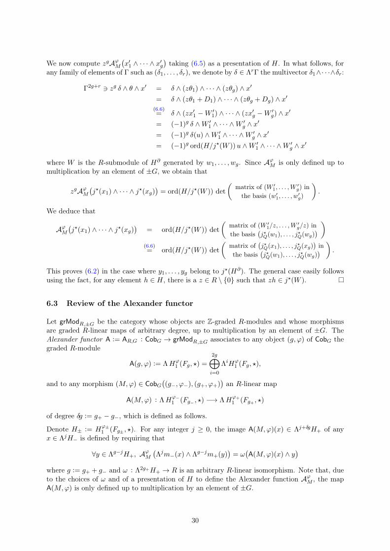
We now compute zgAϕM(x′1 ∧ · · · ∧ x′g

)taking (6.5) as a presentation of H. In what follows, for

any family of elements of Γ such as (δ1, . . . , δr), we denote by δ ∈ ΛrΓ the multivector δ1∧· · ·∧δr:

Γ2g+r 3 zg δ ∧ θ ∧ x′ = δ ∧ (zθ1) ∧ · · · ∧ (zθg) ∧ x′

= δ ∧ (zθ1 +D1) ∧ · · · ∧ (zθg +Dg) ∧ x′

(6.6)= δ ∧ (zx′1 −W ′1) ∧ · · · ∧ (zx′g −W ′g) ∧ x′

= (−1)g δ ∧W ′1 ∧ · · · ∧W ′g ∧ x′

= (−1)g δ(u) ∧W ′1 ∧ · · · ∧W ′g ∧ x′

= (−1)g ord(H/j?(W ))u ∧W ′1 ∧ · · · ∧W ′g ∧ x′

where W is the R-submodule of H∂ generated by w1, . . . , wg. Since AϕM is only defined up tomultiplication by an element of ±G, we obtain that

zgAϕM(j?(x1) ∧ · · · ∧ j?(xg)

)= ord(H/j?(W )) det

(matrix of (W ′1, . . . ,W

′g) in

the basis (w′1, . . . , w′g)

).

We deduce that

AϕM(j?(x1) ∧ · · · ∧ j?(xg)

)= ord(H/j?(W )) det

(matrix of (W ′1/z, . . . ,W

′g/z) in

the basis(j?Q(w1), . . . , j?Q(wg)

))

(6.6)= ord(H/j?(W )) det

(matrix of

(j?Q(x1), . . . , j?Q(xg)

)in

the basis(j?Q(w1), . . . , j?Q(wg)

)).

This proves (6.2) in the case where y1, . . . , yg belong to j?(H∂). The general case easily followsusing the fact, for any element h ∈ H, there is a z ∈ R \ {0} such that zh ∈ j?(W ).

6.3 Review of the Alexander functor

Let grModR,±G be the category whose objects are Z-graded R-modules and whose morphismsare graded R-linear maps of arbitrary degree, up to multiplication by an element of ±G. TheAlexander functor A := AR,G : CobG → grModR,±G associates to any object (g, ϕ) of CobG thegraded R-module

A(g, ϕ) := ΛHϕ1 (Fg, ?) =

2g⊕

i=0

ΛiHϕ1 (Fg, ?),

and to any morphism (M,ϕ) ∈ CobG((g−, ϕ−), (g+, ϕ+)

)an R-linear map

A(M,ϕ) : ΛHϕ−1 (Fg− , ?) −→ ΛH

ϕ+

1 (Fg+ , ?)

of degree δg := g+ − g−, which is defined as follows.

Denote H± := Hϕ±1 (Fg± , ?). For any integer j ≥ 0, the image A(M,ϕ)(x) ∈ Λj+δgH+ of any

x ∈ ΛjH− is defined by requiring that

∀y ∈ Λg−jH+, AϕM(Λjm−(x) ∧ Λg−jm+(y)

)= ω

(A(M,ϕ)(x) ∧ y

)

where g := g+ + g− and ω : Λ2g+H+ → R is an arbitrary R-linear isomorphism. Note that, dueto the choices of ω and of a presentation of H to define the Alexander function AϕM , the mapA(M,ϕ) is only defined up to multiplication by an element of ±G.

30

6.4 Computation of the Alexander functor

Let (M,ϕ) ∈ CobG((g−, ϕ−), (g+, ϕ+)) and keep the notations of Section 6.3. Recall that theMagnus functor assigns to the morphism (M,ϕ) the Lagrangian submodule

Mag(M,ϕ) = cl(kerM) ⊂ H− ⊕H+

where M := (−m−)⊕m+ : H− ⊕H+ → H is induced by the parametrizations m± : Fg± →Mof the top/bottom boundary of M . We also set P := (H− ⊕ H+)/cl(kerM) and denote byp : H− ⊕H+ → P the canonical projection. Since Q⊗R cl(kerM) is a Lagrangian subspace ofH−,Q ⊕ H+,Q, the Q-vector space PQ has dimension g = g− + g+. A transversal of (M,ϕ) isa free submodule W ⊂ H− ⊕ H+ of rank g such that p(W ) ⊂ P generates PQ. Clearly, therealways exists such a W and the R-module p(W ) is free of rank g.

Given a transversal W of (M,ϕ), we can do the following construction. Choose an R-linearisomorphism ω : Λ2g+H+ → R, which induces a Q-linear isomorphism ωQ : Λ2g+H+,Q → Q.Consider the Q-linear map

MagW (M,ϕ) : ΛH−,Q −→ ΛH+,Q

of degree δg = g+ − g− that assigns to any x := x1 ∧ · · · ∧ xj ∈ ΛjH−,Q the multivectorMagW (M,ϕ)(x) ∈ Λj+δgH+,Q defined by the identity

ωQ(MagW (M,ϕ)(x) ∧ y

)= det

(matrix of

(pQ(x1), . . . , pQ(xj), pQ(y1), . . . , pQ(yg−j)

)in

a Q-basis of PQ arising from an arbitrary R-basis of p(W )

)

for any y1, · · · , yg−j ∈ H+,Q. Observe the following:

(i) MagW (M,ϕ) is well-defined up to a multiplication by an element of ±G;

(ii) if W ′ is another transversal of (M,ϕ), then MagW ′(M,ϕ) = dW ′,W MagW (M,ϕ) wheredW ′,W ∈ Q \ {0} is the determinant of a matrix of change of Q-bases of PQ: from anarbitrary R-basis of p(W ) to an arbitrary R-basis of p(W ′).

The next lemma shows that the operator MagW (M,ϕ) carries the same information as thesubmodule Mag(M,ϕ).

Lemma 6.2. Let (M,ϕ), (M ′, ϕ′) ∈ CobG((g−, ϕ−), (g+, ϕ+)). We have Mag(M,ϕ) = Mag(M ′, ϕ′)if, and only if, there exist transversals W,W ′ ⊂ H− ⊕H+ of (M,ϕ), (M ′, ϕ′), respectively, suchthat MagW (M,ϕ) = MagW ′(M

′, ϕ′).

Proof. Assume that Mag(M,ϕ) = Mag(M ′, ϕ). Let W be a transversal of (M,ϕ): then W isalso a transversal of (M ′, ϕ′) and we clearly have MagW (M,ϕ) = MagW (M ′, ϕ).

Conversely, assume thatMagW (M,ϕ) = MagW ′(M′, ϕ′) for some transversalsW,W ′. The canon-

ical isomorphismg⊕

j=0

ΛjH−,Q ⊗Q Λg−jH+,Q'−→ Λg(H−,Q ⊕H+,Q)

can be used to assemble the Q-linear maps

ΛjH−,Q ⊗Q Λg−jH+,Q −→ Q, x⊗ y 7−→ ωQ(MagW (M,ϕ)(x) ∧ y

)

31

defined for all j ∈ {0, . . . , g}, into a single Q-linear map f : Λg(H−,Q ⊕H+,Q)→ Q. This map,which is defined up to multiplication by an element of ±G, satisfies

f(z1 ∧ · · · ∧ zg) = det

(matrix of

(pQ(z1), . . . , pQ(zg)

)in a Q-basis of PQ

arising from an arbitrary R-basis of p(W )

)

for any z1, . . . , zg ∈ H−,Q ⊕H+,Q. It follows that

ker pQ ={z ∈ H−,Q ⊕H+,Q : f(z ∧ ·) = 0 ∈ HomQ

(Λg−1(H−,Q ⊕H+,Q), Q

)}.

Similarly, we have

ker p′Q ={z ∈ H−,Q ⊕H+,Q : f ′(z ∧ ·) = 0 ∈ HomQ

(Λg−1(H−,Q ⊕H+,Q), Q

)}

where p′ : H−⊕H+ → P ′ := (H−⊕H+)/Mag(M ′, ϕ′) is the canonical projection and f ′ is definedfrom MagW ′(M

′, ϕ′) in the same way as f is defined from MagW (M,ϕ). Thus the assumptionMagW (M,ϕ) = MagW ′(M

′, ϕ′) implies that f = f ′, and we conclude that

Mag(M,ϕ) = (ker pQ) ∩ (H− ⊕H+) = (ker p′Q) ∩ (H− ⊕H+) = Mag(M ′, ϕ′).

We now give the main result of this section, showing that the Alexander functor can be factorizedinto two parts. One part is scalar and is a kind of relative Alexander polynomial, while theother part is the operator version of the Magnus functor and, so, is invariant under homologyconcordance (Proposition 4.5).

Theorem 6.3. Let (M,ϕ) ∈ CobG((g−, ϕ−), (g+, ϕ+)) with transversal W . Then

A(M,ϕ) = ord(H/M(W )

)·MagW (M,ϕ)

∣∣ΛH−

where H = Hϕ1 (M,?), H± = H

ϕ±1 (Fg± , ?) and M = (−m−)⊕m+ : H− ⊕H+ → H.

Proof. Two cases have to be distinguished. If MQ : H−,Q ⊕H+,Q → HQ is not surjective, thenthe map j?Q : Q⊗R Hϕ

1 (∂M, ?)→ HQ induced by the inclusion is not surjective; it follows fromthe first part of Lemma 6.1 that AϕM = 0, which implies that A(M,ϕ) = 0, and it also follows thatdimHQ > g; but dim(Q ⊗R M(W )) ≤ dimWQ = g, and we deduce that ord

(H/M(W )

)= 0.

If MQ : H−,Q ⊕ H+,Q → HQ is surjective, then the result follows from the second part ofLemma 6.1.

Remark 6.4. Consider the monoid of homology cobordisms Cϕ(Fg) introduced in Section 5.1.Here g ≥ 1 and ϕ : H1(Fg) → G is a group homomorphism. It follows from Lemma 4.6 thatW± := H± is a transversal of (M,ϕ) for any M ∈ Cϕ(Fg). On the one hand, we have

ord(H/M(W±)

)= ord

(H/m±(H±)

)= ord Hϕ

1 (M,∂±M) ∈ (R \ {0})/±G

which we denote by ∆(M,∂±M) and view as a relative version of the Alexander polynomial. Onthe other hand, it follows from the definitions that

MagW+(M,ϕ) = Λ

(rϕ(M)

)and MagW−(M,ϕ) = det(rϕ(M)

)−1 · Λ(rϕ(M)

)

where rϕ(M) ∈ AutQ(HQ) is the Magnus representation of M . By Theorem 6.3, we get

A(M,ϕ) = ∆(M,∂+M) · Λ(rϕ(M)

)= ∆(M,∂−M) det(rϕ(M)

)−1 · Λ(rϕ(M)

)

which is already proved in [FM15, Proposition 7.3 & Example 9.6] using the theory of Reide-meister torsions. This example shows that the “non-Magnus” part of A(M,ϕ) in the factorizationformula of Theorem 6.3 is not invariant under homology concordance. (See [FM15, Remark 7.5].)

32

6.5 The free case

We keep the notations of Section 6.4, which we specialize to the case where the R-moduleP = (H− ⊕H+)/cl(kerM) is free. (For instance, this condition is certainly satisfied if G = {1}and R = Z.) Then a natural choice of transversal for (M,ϕ) is the image of an arbitrary sections : P → H− ⊕ H+ of the projection p. Since p(s(P )) = P , the map Mags(P )(M,ϕ) does notdepend on the choice of s, and it can be described as follows. Because Mag(M,ϕ) = cl(kerM)is then a direct summand of the free R-module H− ⊕ H+, it is a finitely-generated projectivemodule so that, by a classical result of Quillen and Suslin, it is free. Thus, by Plücker embedding,we can consider instead the multivector

Pl(Mag(M,ϕ)) := e1 ∧ · · · ∧ eg ∈ Λg(H− ⊕H+)/±G

where (e1, . . . , eg) is an arbitrary basis ofMag(M,ϕ). Through the sequence of isomorphisms

Λg(H− ⊕H+) 'g⊕

k=0

ΛkH− ⊗ Λg−kH+ 'g⊕

k=0

Hom(Λ2g−−kH−, R

)⊗ Λg−kH+

'g⊕

k=0

Hom(Λ2g−−kH−,Λ

g−kH+

)

(whose second one is determined by the choice of an isomorphism Λ2g−H− ' R), the multivectorPl(Mag(M,ϕ)) can be viewed as an R-linear map Pl(Mag(M,ϕ)) : ΛH− → ΛH+ which is well-defined up to multiplication by an element of ±G. It can be verified that (for an appropriatechoice of signs in the above sequence of isomorphisms)

Mags(P )(M,ϕ) = Q⊗R Pl(Mag(M,ϕ)

)

and we deduce the following from Theorem 6.3.

Corollary 6.5. Let (M,ϕ) ∈ CobG((g−, ϕ−), (g+, ϕ+)) be such that P = (H− ⊕H+)/cl(kerM)is free, where H = Hϕ

1 (M,?), H± = Hϕ±1 (Fg± , ?) and M = (−m−)⊕m+ : H−⊕H+ → H. Then

A(M,ϕ) = ord(H/M(W )

)· Pl(Mag(M,ϕ)

)

where W ⊂ H− ⊕H+ is an arbitrary free submodule of rank g which projects onto P .

Remark 6.6. The use of the Plücker embedding to transform submodules into linear operatorsalready appears in [Don99] for G := {1} and R := R. (See Section 5.3 in this connection.)

A Glossary

A monoidal category is a category C with a monoidal structure, which consists of

� a bifunctor � : C× C→ C, called the tensor product,

� an object I of C, called the unit object,

� a natural isomorphism AX ,Y,Z : (X � Y) � Z → X � (Y � Z), called the associativityconstraint, for any objects X ,Y,Z of C,

33

� a natural isomorphism LX : I � X → X (respectively, RX : X � I → X ), called the left(respectively, right) unit constraint, for any object X of C,

satisfying two kinds of coherence conditions: see [ML98, §VII.1]. If all the natural isomorphismsAX ,Y,Z , LX , and RX are identities, the monoidal category C is said to be strict.

Let (C,�, I, A, L,R) and (C′,�′, I ′, A′, L′, R′) be monoidal categories. A monoidal functor fromC to C′ is a functor F : C→ C′ coming with

� a natural transformation TX ,Y : F (X ) �′ F (Y)→ F (X � Y), for any objects X ,Y of C,

� a morphism U : I ′ → F (I) in C′,

satisfying three kinds of coherence conditions which involve the associativity/unit constraints ofC and C′: see [ML98, §XI.2]. If U is an isomorphism (respectively, the identity) and if TX ,Y isa natural isomorphism (respectively, the identity), then the monoidal functor F is said to bestrong (respectively, strict).

Acknowledgements. The authors would like to thank the referee for helpful comments and sug-gestions. The third author is partially supported by the Spanish Ministry of Education (grantsMTM2013-45710-C2-1-P and MTM2016-76868-C2-2-P), by the “Grupo de Geometría del Go-bierno de Aragón” and by the European Social Fund.

References

[Arc10] Jana Archibald, The Multivariable Alexander Polynomial on Tangles, ProQuest LLC, AnnArbor, MI, 2010, Thesis (Ph.D.)–University of Toronto (Canada).

[BCF15] Stephen Bigelow, Alessia Cattabriga, and Vincent Florens, Alexander representation of tangles,Acta Math. Vietnam. 40 (2015), no. 2, 339–352.

[Bir74] Joan S. Birman, Braids, links, and mapping class groups, Princeton University Press, Princeton,N.J.; University of Tokyo Press, Tokyo, 1974, Annals of Mathematics Studies, No. 82.

[Bla57] Richard C. Blanchfield, Intersection theory of manifolds with operators with applications toknot theory, Ann. of Math. (2) 65 (1957), 340–356.

[CFK11] Jae Choon Cha, Stefan Friedl, and Taehee Kim, The cobordism group of homology cylinders,Compos. Math. 147 (2011), no. 3, 914–942. MR 2801405

[CST16] James Conant, Robert Schneiderman, and Peter Teichner, Geometric filtrations of string linksand homology cylinders, Quantum Topol. 7 (2016), no. 2, 281–328. MR 3459962

[CT05] David Cimasoni and Vladimir Turaev, A Lagrangian representation of tangles, Topology 44(2005), no. 4, 747–767.

[CT06] , A Lagrangian representation of tangles. II, Fund. Math. 190 (2006), 11–27.

[CY99] Louis Crane and David Yetter, On algebraic structures implicit in topological quantum fieldtheories, J. Knot Theory Ramifications 8 (1999), no. 2, 125–163.

[DF16] Celeste Damiani and Vincent Florens, Alexander ivariants of ribbon tangles and planar algebras,arXiv:1602.06191 (2016).

[Don99] S. K. Donaldson, Topological field theories and formulae of Casson and Meng-Taubes, Proceed-ings of the Kirbyfest (Berkeley, CA, 1998), Geom. Topol. Monogr., vol. 2, Geom. Topol. Publ.,Coventry, 1999, pp. 87–102.

34

[FM15] Vincent Florens and Gwénaël Massuyeau, A functorial extension of the abelian Reidemeistertorsions of three-manifolds, Enseign. Math. 61 (2015), no. 1, 161–210.

[FN91] Charles Frohman and Andrew Nicas, The Alexander polynomial via topological quantum fieldtheory, Differential geometry, global analysis, and topology (Halifax, NS, 1990), CMS Conf.Proc., vol. 12, Amer. Math. Soc., Providence, RI, 1991, pp. 27–40.

[FN94] , An intersection homology invariant for knots in a rational homology 3-sphere, Topology33 (1994), no. 1, 123–158.

[GL05] Stavros Garoufalidis and Jerome Levine, Tree-level invariants of three-manifolds, Massey prod-ucts and the Johnson homomorphism, Graphs and patterns in mathematics and theoreticalphysics, Proc. Sympos. Pure Math., vol. 73, Amer. Math. Soc., Providence, RI, 2005, pp. 173–203. MR 2131016

[HLW15] Jennifer Hom, Tye Lindman, and Liam Watson, The Alexander module, Seifert forms andcategorification, arXiv:1501.04866 (2015).

[HM12] Kazuo Habiro and Gwénaël Massuyeau, From mapping class groups to monoids of homologycobordisms: a survey, Handbook of Teichmüller theory. Volume III, IRMA Lect. Math. Theor.Phys., vol. 17, Eur. Math. Soc., Zürich, 2012, pp. 465–529.

[Ker03a] Thomas Kerler, Homology TQFT’s and the Alexander-Reidemeister invariant of 3-manifoldsvia Hopf algebras and skein theory, Canad. J. Math. 55 (2003), no. 4, 766–821.

[Ker03b] , Towards an algebraic characterization of 3-dimensional cobordisms, Diagrammaticmorphisms and applications (San Francisco, CA, 2000), Contemp. Math., vol. 318, Amer.Math. Soc., Providence, RI, 2003, pp. 141–173.

[KLW01] Paul Kirk, Charles Livingston, and Zhenghan Wang, The Gassner representation for stringlinks, Commun. Contemp. Math. 3 (2001), no. 1, 87–136.

[LD92] J.-Y. Le Dimet, Enlacements d’intervalles et représentation de Gassner, Comment. Math. Helv.67 (1992), no. 2, 306–315.

[Les98] Christine Lescop, A sum formula for the Casson-Walker invariant, Invent. Math. 133 (1998),no. 3, 613–681.

[Mag39] Wilhelm Magnus, On a theorem of Marshall Hall, Ann. of Math. (2) 40 (1939), 764–768.

[ML98] Saunders Mac Lane, Categories for the working mathematician, second ed., Graduate Texts inMathematics, vol. 5, Springer-Verlag, New York, 1998. MR 1712872

[Mor93] Shigeyuki Morita, Abelian quotients of subgroups of the mapping class group of surfaces, DukeMath. J. 70 (1993), no. 3, 699–726.

[Mor08] , Symplectic automorphism groups of nilpotent quotients of fundamental groups of sur-faces, Groups of diffeomorphisms, Adv. Stud. Pure Math., vol. 52, Math. Soc. Japan, Tokyo,2008, pp. 443–468. MR 2509720

[Pap75] C. D. Papakyriakopoulos, Planar regular coverings of orientable closed surfaces, Knots, groups,and 3-manifolds (Papers dedicated to the memory of R. H. Fox), Princeton Univ. Press, Prince-ton, N.J., 1975, pp. 261–292. Ann. of Math. Studies, No. 84.

[Per06] Bernard Perron, A homotopic intersection theory on surfaces: applications to mapping classgroup and braids, Enseign. Math. (2) 52 (2006), no. 1-2, 159–186.

[Rei39] Kurt Reidemeister, Durchschnitt und Schnitt von Homotopieketten, Monatsh. Math. Phys. 48(1939), 226–239.

[Sak07] Takuya Sakasai, The symplecticity of the Magnus representation for homology cobordisms ofsurfaces, Bull. Austral. Math. Soc. 76 (2007), no. 3, 421–431.

[Sak08] , The Magnus representation and higher-order Alexander invariants for homology cobor-disms of surfaces, Algebr. Geom. Topol. 8 (2008), no. 2, 803–848.

35

[Sak12] , A survey of Magnus representations for mapping class groups and homology cobordismsof surfaces, Handbook of Teichmüller theory. Volume III, IRMA Lect. Math. Theor. Phys.,vol. 17, Eur. Math. Soc., Zürich, 2012, pp. 531–594.

[Suz03] Masaaki Suzuki, On the Magnus representation of the mapping class group, Proceedings ofthe Winter Workshop of Topology/Workshop of Topology and Computer (Sendai, 2002/Nara,2001), vol. 9, 2003, pp. 77–80.

[Suz05] , Geometric interpretation of the Magnus representation of the mapping class group,Kobe J. Math. 22 (2005), no. 1-2, 39–47.

[Tur78] V. G. Turaev, Intersections of loops in two-dimensional manifolds, Mat. Sb. 106(148) (1978),no. 4, 566–588.

Vincent FlorensLMA, Université de Pau & CNRSAvenue de l’Université64000 Pau, Francevincent.florens@univ-pau.fr

Gwénaël MassuyeauIRMA, Université de Strasbourg & CNRS and IMB, Université de Bourgogne & CNRS7 rue René Descartes 9 avenue Alain Savary67084 Strasbourg, France 21000 Dijon, Francemassuyeau@math.unistra.fr

Juan Serrano de RodrigoDpto. de Matemáticas, Universidad de ZaragozaCalle Pedro Cerbuna 1250009 Zaragoza, Spainserrano.de.rodrigo@gmail.com

36