Using Self-Organizing Maps to infill missing data in hydro...
19
This is a repository copy of Using Self-Organizing Maps to infill missing data in hydro-meteorological time series from the Logone catchment, Lake Chad basin . White Rose Research Online URL for this paper: http://eprints.whiterose.ac.uk/100773/ Version: Accepted Version Article: Nkiaka, E, Nawaz, NR and Lovett, JC (2016) Using Self-Organizing Maps to infill missing data in hydro-meteorological time series from the Logone catchment, Lake Chad basin. Environmental Monitoring and Assessment, 188. 400. ISSN 0167-6369 https://doi.org/10.1007/s10661-016-5385-1 (c) 2016, Springer International Publishing Switzerland. This is an author produced version of a paper published in Environmental Monitoring and Assessment. Uploaded in accordance with the publisher's self-archiving policy. The final publication is available at Springer via: http://dx.doi.org/10.1007/s10661-016-5385-1 [email protected] https://eprints.whiterose.ac.uk/ Reuse Unless indicated otherwise, fulltext items are protected by copyright with all rights reserved. The copyright exception in section 29 of the Copyright, Designs and Patents Act 1988 allows the making of a single copy solely for the purpose of non-commercial research or private study within the limits of fair dealing. The publisher or other rights-holder may allow further reproduction and re-use of this version - refer to the White Rose Research Online record for this item. Where records identify the publisher as the copyright holder, users can verify any specific terms of use on the publisher’s website. Takedown If you consider content in White Rose Research Online to be in breach of UK law, please notify us by emailing [email protected] including the URL of the record and the reason for the withdrawal request.
Transcript of Using Self-Organizing Maps to infill missing data in hydro...

This is a repository copy of Using Self-Organizing Maps to infill missing data in hydro-meteorological time series from the Logone catchment, Lake Chad basin.
White Rose Research Online URL for this paper:http://eprints.whiterose.ac.uk/100773/
Version: Accepted Version
Article:
Nkiaka, E, Nawaz, NR and Lovett, JC (2016) Using Self-Organizing Maps to infill missing data in hydro-meteorological time series from the Logone catchment, Lake Chad basin. Environmental Monitoring and Assessment, 188. 400. ISSN 0167-6369
https://doi.org/10.1007/s10661-016-5385-1
(c) 2016, Springer International Publishing Switzerland. This is an author produced versionof a paper published in Environmental Monitoring and Assessment. Uploaded in accordance with the publisher's self-archiving policy. The final publication is available at Springer via: http://dx.doi.org/10.1007/s10661-016-5385-1
[email protected]://eprints.whiterose.ac.uk/
Reuse
Unless indicated otherwise, fulltext items are protected by copyright with all rights reserved. The copyright exception in section 29 of the Copyright, Designs and Patents Act 1988 allows the making of a single copy solely for the purpose of non-commercial research or private study within the limits of fair dealing. The publisher or other rights-holder may allow further reproduction and re-use of this version - refer to the White Rose Research Online record for this item. Where records identify the publisher as the copyright holder, users can verify any specific terms of use on the publisher’s website.
Takedown
If you consider content in White Rose Research Online to be in breach of UK law, please notify us by emailing [email protected] including the URL of the record and the reason for the withdrawal request.

1
Nkiaka, E., Nawaz, N.R. & Lovett, J.C. 2016. Using self-organizing maps to infill missing 1
data in hydro-meteorological time series from the Logone catchment, Lake Chad basin. 2
Environmental Monitoring and Assessment. 3
DOI 10.1007/s10661-016-5385-1 4
5
Using Self-Organizing Maps to infill missing data in hydro-meteorological time series from 6
the Logone catchment, Lake Chad basin 7
8
E. Nkiaka1, N.R. Nawaz1 and J.C. Lovett1 9
1School of Geography, University of Leeds: 10
Correspondence to: E. Nkiaka ([email protected]) 11
12
Abstract 13
Hydro-meteorological data is an important asset that can enhance management of water resources. 14
But existing data often contains gaps, leading to uncertainties and so compromising their use. 15
Although many methods exist for infilling data gaps in hydro-meteorological time series, many of 16
these methods require inputs from neighbouring stations, which are often not available, while other 17
methods are computationally demanding. Computing techniques such Artificial Intelligence can 18
be used to address this challenge. Self-Organizing Maps (SOMs), which are a type of Artificial 19
Neural Network, was used for infilling gaps in a hydro-meteorological time series in a Sudano-20
Sahel catchment. The coefficients of determination obtained were all above 0.75 and 0.65 while 21
the average topographic error was 0.008 and 0.02 for rainfall and river discharge time series 22
respectively. These results further indicate that SOMs are a robust and efficient method for infilling 23
missing gaps in hydro-meteorological time series. 24
25
Keywords: Artificial Neural Networks, hydro-meteorological data, infilling missing data, Logone 26
catchment, Self-Organizing Maps, 27
28
1) Introduction 29
Economic progress, rising standard of living, growing populations and expansion of 30
commercial agriculture in developing countries is putting increasing pressure on fresh water 31
resources (WWAP, 2015). At the same time climate extremes such as droughts and floods are 32
becoming more frequent (Coumou & Rahmstorf, 2012). Better informed water resource 33
management is needed to respond to demand and climate variability. A major requirement for 34
planning is the availability of good quality and long term hydro-meteorological data. This data 35
provides indicators of past hydro-climatic behaviour of a region/catchment and is fundamental to 36
the development of models for prediction of system behaviour (Harvey et al., 2012). 37
Existing hydro-meteorological time series used for planning and management decisions 38
often contains missing observations, particularly in developing countries. The gaps are caused by 39
many reasons, including equipment failure, destruction of equipment by natural catastrophes such 40
as floods, war and civil unrest, mishandling of observed records by personnel or loss of files 41
containing the data in a computer system (Elshorbagy et al., 2000). The presence of gaps, even if 42
there are very short, in a hydro-meteorological time series can hinder calculation of important 43
statistical parameters as data patterns maybe hidden. This can compromise their use for water 44

2
resources planning as it increases the level of uncertainty in the datasets (Ng and Panu, 2010; 45
Campozano et al., 2014). This problem is particularly acute in the Sudano-Sahel region where 46
rainfall is highly variable in both space and time, meteorological and flow gauging stations are 47
scarce and the available datasets are riddled with gaps. 48
Several methods exist for infilling gaps in hydro-meteorological time series. However, the 49
application of each method depends on a range of factors including the information available for 50
that station; additional datasets from neighbouring stations; the percentage of gaps present within 51
the time series to be infilled; the season within which the gaps are present; the length of the existing 52
data series; and the type of application that the infilled series will be used for (Mwale et al., 2012). 53
These infilling methods range from simple techniques such as linear interpolation, Inverse Distance 54
Weighting (IDW) and Thiessen polygons; to more complicated advanced techniques such as time 55
series models, Markov models, Global Imputation, Multiple Regression models, Artificial 56
Intelligence (Kalteh & Hjorth, 2009; Presti et al., 2010; Ismail et al., 2012; Mwale et al., 2012; 57
Campozano et al., 2014). 58
Most of the methods, require additional input data from neighbouring stations in order to 59
produce reliable results and these additional inputs are often not available. Furthermore, some of 60
the methods are time consuming and demand subtantial computer power for simulation because of 61
the complicated algorithms involved (Presti et al., 2010). Some methods also require that the time 62
series be split into different seasons to obtain reliable results. Although these challenges could be 63
overcome by using numerical models (e.g. hydrological models); models also demand high data 64
inputs and cannot be applied to many stations at the same time due to parameter calibration 65
requirements which are site specific and consequently results cannot be transferred to other stations 66
even within the same catchment (Harvey et al., 2012). 67
Some of these challenges can be overcome by using computing techniques such as Artificial 68
Intelligence (AI) (Daniel et al., 2011). In this class of technique, the most promising approaches 69
include Artificial Neural Networks (ANN), Fuzzy Logic (FL) and Genetic Algorithms (GA). The 70
application of Artificial Intelligence in hydrology and water resources management is well 71
established (ASCE 2000; Kingston et al., 2008a, 2008b; Daniel et al., 2011). Among the AI class 72
of models, ANNs are probably the most popular as these use available data to learn about the 73
behaviour of a time series. In addition, they possess capabilities for modelling complex nonlinear 74
systems; do not require prior knowledge of the system process(s) under study and are robust even 75
in the presence of missing observations in the time series (Mwale et al., 2012). The main advantage 76
of ANNs over conventional methods is their ability to model physical processes without the need 77
for detailed information of the system (Daniel et al., 2011); and they have often been used for 78
infilling gaps in hydro-meteorological time series (Kalteh & Hjorth, 2009; Dastorani et al., 2010; 79
Adeloye et al., 2012; Ismail et al., 2012; Mwale et al., 2012; Mwale et al., 2014; Kim et al., 2015). 80
Within the ANN family, the Multilayer Perceptron (MLP) is one of the most widely used 81
for infilling gaps in hydro-meteorological time series (Kalteh & Hjorth, 2009; Dastorani et al., 82
2010; Mwale et al., 2012; Mwale et al., 2014; Kim et al., 2015). Although MLP is robust for 83
performing this task, it usually demands a long time series for training; and if part of the data to be 84
used for training is missing, additional pre-processing of the time series will have to be carried out 85
to provide estimates in the input space before the training can begin (Rustum & Adeloye, 2007; 86
Mwale et al., 2012). This therefore limits application in situations where significant portions of the 87
time series to be used for training have incomplete data; or for short time series as the data may 88
3
not be sufficient for training. It is also computationally intensive and needs additional storage 89
memory (Kalteh et al., 2008). 90
Another member of the class of ANNs known as Self-Organizing Maps (SOMs), which is 91
a competitive and unsupervised ANN, is becoming popular for infilling gaps in hydro-92
meteorological times series and has been shown to outperform ANNs-MLP (Kalteh & Hjorth, 93
2009; Mwale et al., 2014; Kim et al., 2015). Many studies have successfully applied SOMs for 94
infilling gaps in hydro-meteorological time series with satisfactory results (Kalteh & Hjorth, 2009; 95
Rustum & Adeloye, 2011; Adeloye et al., 2012; Mwale et al., 2012; Mwale et al., 2014; Kim et 96
al., 2015). 97
Self-Organizing Maps (SOMs) were first introduced by Kohonen, (1995, 1997). The 98
success of their application in other research disciplines led to their wide application in water 99
resources processes and systems research especially for data mining, infilling of missing data, 100
estimation and flow forecasting, clustering etc. (Kalteh et al., 2008). This is due to their ability to 101
convert nonlinear statistical relationships between high dimensional data onto a low dimensional 102
display (Ismail et al., 2012). Data points that show similar characteristics are placed closed to each 103
other or clustered together in the output space. This mapping approach does a quasi-preservation 104
of the most important topological and metric relationship of the original data (Rustum & Adeloye, 105
2007). Adeloye et al. (2012) asserted that, the ability of SOMs to cluster data together makes them 106
robust for data mining and infilling datasets with gaps and outliers as the gaps/outliers are replaced 107
by their features in the map. The SOMs algorithm generally executes assigned tasks using an 108
unsupervised and competitive learning approach to discover patterns in the data (Kalteh & 109
Berndtsson, 2007) thus, the whole process in entirely data driven. A SOM is made up of two layers: 110
a multi-dimensional input layer and an output layer. Both layers are fully connected by adjustable 111
weights and the output layer is made up of neurons arranged in a two dimensional grid of nodes 112
(Figure 1). Each neuron in the output layer of the SOM contains exactly the same set of variables 113
contained in the input vectors. Despite its wide application for infilling missing data in many 114
studies around the world, it has rarely been used Africa in general and the Sudano-Sahel region in 115
particular. 116
A Self-Organizing Maps approach was applied to infill missing data in monthly rainfall and 117
daily river discharge time series from January 1950 to December 2007 in the Logone river 118
catchment covering Cameroon, the Central Africa Republic and Chad. Infilling of missing gaps in 119
hydro-meteorological time series usually precedes most hydro-climatic studies (Kashani & 120
Dinpashoh, 2012), and this work is part of an on-going research project to assess the vulnerability 121
of this catchment to drought and flood events under anticipated increased climate variability. 122
The paper is structured as follows: Section 2 describes the data and methodology used in 123
the study. In Section 3 the results obtained are presented and discussed. Section 4 gives a general 124
summary and conclusion of the study. 125
126
2) Methodology 127
2.1) Study area 128
The Logone catchment is part of the greater Lake Chad basin. It lies between latitude 6˚-12˚N 129
and longitude 13˚-16˚E and is a transboundary catchment in the Sudano-Sahel transitional zone in 130
Central Africa with an estimated catchment area of 86,500 km2 (Figure 1). 131

4
The Logone River has its source in Cameroon through the Mbere and Vina Rivers, which flow 132
from the northeastern slopes of the Adamawa plateau. It is joined in Lai by the Pende River from 133
the Central Africa Republic and flows from south to north to join the Chari River in Ndjamena 134
(Chad) and continue flowing in a northward direction before finally emptying into Lake Chad. The 135
climate in the catchment is characterized by high spatial variability and is dominated by seasonal 136
changes in the tropical continental air mass (the Harmattan) and the marine equatorial air mass 137
(monsoon) (Candela et al., 2014). 138
139
2.2) Data Sources 140
Monthly gauge rainfall was obtained from SIEREM (Boyer et al., 2006) available for 18 141
stations covering the period 1950-2000 while daily river discharge data was obtained from the 142
Lake Chad Basin Commission (LCBC). Discharge time series are available for the stations of Lai, 143
Bongor, Katoa and Logone Gana covering the period 1973-1998 for Lai and 1983-2007 for the 144
rest of the stations. 145
146
2.3) Implementation of the SOM Algorithm 147
A SOM algorithm is implemented in a series of steps. 148
The multi-dimensional input data is first standardized to make sure that very high or low 149
value variables do not dominate the map. Since SOMs use Euclidian metrics to measure distances 150
between vectors, standardization gives equal weight to all the input variables (Vesanto et al., 2000). 151
In this analysis, data was not standardized because rainfall and river discharge time series were 152
trained separately. 153
The input vector is then chosen at random and presented to each of the individual neurons for 154
comparison with their weight vectors in order to identify the weight vector most similar to the 155
presented input vector. The identification uses the Euclidian distance defined as: 156
157
経沈 噺 彪布 兼珍岫捲珍 伐 拳沈珍岻態津珍退怠 ┹ 件 噺 な┸ に┸ ぬ ┼ ┻ 警 岫な岻 158
159
Where: 160
Di = Euclidian distance between the input vector and the weight vector i; xj = j element of the 161
current vector; wij = j element of the weight vector I; n = the dimension of the input vector; mj = 162
“mask”. 163
When the input vector contains missing elements, the mask is set to zero for such elements and 164
because of this, the SOM algorithm can conveniently handle missing elements in the input vector. 165
The neuron whose vector closely matches the input vector (i.e. with Di minimum) is chosen as the 166
winning node or best matching unit (BMU). 167
After finding the BMU, the weight vector of the winner neuron is adjusted so that the BMU and 168
its adjacent neurons move closer to the input vectors in the input space, thereby increasing the 169
agreement between the input vector and the weight vector. This adjustment is carried out using the 170
following equation: 171
172 拳痛岫建 髪 な岻 噺 拳痛岫建岻 髪 糠岫建岻月頂沈岷捲岫建岻 伐 拳痛岫建岻峅 岫に岻 173
174

5
Where: wt = element of the weight vector; t = time; Į(t) = learning rate at time t; hci(t) = 175
neighbourhood function centred in the winner unit c at time t. 176
From here, each node in the map develops the ability to recognize input vectors that are similar to 177
itself. This ability is referred to as self-organizing as no external information is added for this 178
process to take place. The learning procedure continues until the SOM algorithm converges. 179
Generally, the learning rate decreases monotonically as the number of iterations increase as shown 180
by the following equation: 181
182
糠岫建岻 噺 糠待岫待┻待待泰底轍 岻禰畷 岫ぬ岻 183
184
Where: Į(t)= learning rate; Į0 = initial learning rate; T = training length 185
The neighbourhood function used is in this analysis is Gaussian centred in the winner unit c, 186
calculated as: 187
188 月頂沈岫建岻 噺 exp 班伐 弁】堅頂 伐 堅沈】弁態岷に購態岫建岻峅 藩 岫ね岻 189
190
Where: 191
hci(t) = neighbourhood function centred in the winner unit c at time t; rc and ri = positions of nodes 192
c and i on the SOM grid; ı(t) = neighbourhood radius which also decreases monotonically as the 193
number of iterations increases. 194
The quality of the trained SOM is measured by the total average quantization error and total 195
topographic error. The average quantization error is a measure of how good the map fits the input 196
data (it measures the average distance between each data vector and its Best Matching Unit 197
(BMU)). The smaller the quantization error, the smaller the average of the distance from the vector 198
data to the prototypes, meaning that the data vectors are closer to its prototypes; it is a positive real 199
number with a value close to zero indicating a good fit between the input and the map. The 200
quantization error is calculated as: 201
202 圏勅 噺 な軽 布押隙沈 伐 激沈頂押朝沈退怠 岫の岻 203
Where: qe = quantization error; N = number of input vectors used to train the map; Xi = ith data 204
sample or vector; Wc =prototype vector of the best matching unit for X; ||.|| = denotes the Euclidian 205
distance. 206
Topographic error measures how well the topology of the data is preserved by the map by 207
considering the map structure. The lower the topographic error, the better the SOM preserves the 208
topology of the data. It is a positive real number between 0 and 1 with a value close to 0 indicating 209
good quality. It is calculated as: 210 建勅 噺 な軽 布 憲岫隙沈岻 岫は岻朝沈退怠 211
Where: te = topographic error; N = number of input vectors used to train the map; 212
ui = binary integer such that it is equal to 1 if the first and second BMU for Xi are not adjacent 213
units; otherwise it is zero. 214

6
Since there is always a trade-off between which of the two can be minimized at the expense of the 215
other, in this study, effort was focused on reducing the topographic error to ensure that the infilled 216
values reflect the seasonal trend of the different time series. The coefficient of determination (R2) 217
was used to check the quality of the newly generated time series. R2 gives the proportion of the 218
variance of one variable that is predictable from the other variable and varies between 0 and 1. R2 219
is calculated as: 220
221 迎態 噺 デ 岷岫捲沈 伐 捲違岻岫検沈 伐 検博岻津沈退怠 峅デ 岷岫捲沈 伐 捲違岻態峅 デ 岷岫検沈 伐 捲違岻態峅津沈退怠 津沈退怠 岫ば岻 222
223
Where: xi = the ith observed value; yi = the ith trained value; 捲違= the mean of observed value; 検博 224
= the mean of the trained value; n = the number of observations. 225
226
2.4) Setting of SOM algorithm parameters 227
According to Gabrielsson & Gabrielsson, (2006), the radius of the SOM should be chosen 228
wide enough at the beginning of the learning process so that the map can be ordered globally as 229
the radius decreases monotonically with time. To determine the optimum number of neurons, if M 230
is the total number of input elements, Garcia and Gonzalez (2004), propose that the number of 231
neurons in the output can be calculated as: 232
233 軽 噺 のヂ警 岫ぱ岻 234
Where: M = total number of samples and N = the number of neurons. 235
Once N is known, Garcia and Gonzalez, (2004) further propose that the number of rows and 236
columns of N can be calculated by: 237
238 健怠健態 噺 俵結な結に 岫ひ岻 239
240
Where l1 and l2 are the number of rows and columns respectively, e1 is the biggest eigenvalue of 241
the training data set and e2 is the second biggest eigenvalue. 242
In the initialization phase of the algorithm, since the learning process involve in the 243
computation of a feature map is a stochastic process, according to Gabrielsson & Gabrielsson, 244
(2006) the accuracy of the map depends on the number of iterations executed by the SOM 245
algorithm. These authors recommend that for good statistical accuracy, the number of iterations 246
should be at least 500 times the number of network nodes. In this study, the random initialization 247
option was used as it is recommended for hydrological applications e.g. (Kalteh et al., 2008), while 248
the default parameters set by the SOM software for map size and lattice (rows and columns) were 249
adopted that were exactly the same as using equations (8) and (9). 250
251
The basic steps required to complete the infilling process consists of the following: 252
1) Data gathering and normalization: The data to be infilled (e.g. rainfall and discharge time 253
series) is assembled together and standardized; these are the depleted input vectors; 254
2) Training: The depleted input vector (data matrix) is introduced to the iterative training 255
procedure to form the SOM. At the beginning of the training, weight vectors must be 256
initialized by using either a random or a linear initialization method. The process of 257

7
comparison and adjustment continues until the optimal number of iteration is reached or 258
the specified error criteria are attained. 259
3) Extracting information from the trained SOM: Check all the minimum Euclidian distances 260
and isolate the SOM’s BMU for the depleted input vector (i.e. with missing values). The 261
BMU identified in this step is a node of trained SOM and thus has the full complement of 262
the missing values; 263
4) Replacement of missing values: Replace the missing values of the input depleted vector by 264
their corresponding values in BMU identified in step 3 above. 265
266
2.5) Application of SOM 267
For the application of the SOM algorithm for infilling of missing data in this analysis, a 268
SOM toolbox developed at Helsinki University of Technology Finland 269
(www.cis.hut.fi/projects/somtoolbox/) was used in the Matlab® 2014b environment and a batch 270
training algorithm was adopted. Due to the fact both datasets (rainfall and river discharge) had 271
different time-steps, each of the datasets were trained separately. The data was presented in 272
columns with each column representing measurements from each station. The entries without data 273
were recorded as NaN (Not a Number) to meet Matlab® data entry requirements. To train all the 274
data together in a single simulation, the data entries should overlap such that there is no single 275
day/month for all the stations with no data entry. 276
The stations with the longest period of continuous missing observation were Katoa with 277
1418 consecutive days (01/04/1997-18/025/2001) approximately 4 years and Lai with 1200 278
consecutive days (31/01/1979-15/05/1982), approximately 3 years. Donomanga had the longest 279
period of missing monthly rainfall observations. 280
281
3) Results and Discussion 282
Initial simulation results using discharge time series produced an average topographic error 283
of 0.04 and a visual inspection of the time series was carried out to check the seasonal trends. 284
Sporadic cases of numerical instability were noticed especially in portions of the time series with 285
extensive gaps where infilling was done. In some cases, high flow values were observed in the dry 286
season and low flow values observed in the rainy season. This was not logical as periods of high 287
flows could not be followed by a single day of abrupt low flow and vice versa. These values were 288
manually deleted for all the stations and a second simulation was performed using the same initial 289
parameters. After this second simulation, these abnormalities disappeared and the average 290
topographic error reduced to 0.02. Results of the overall performance of the model are shown in 291
Table 1. 292
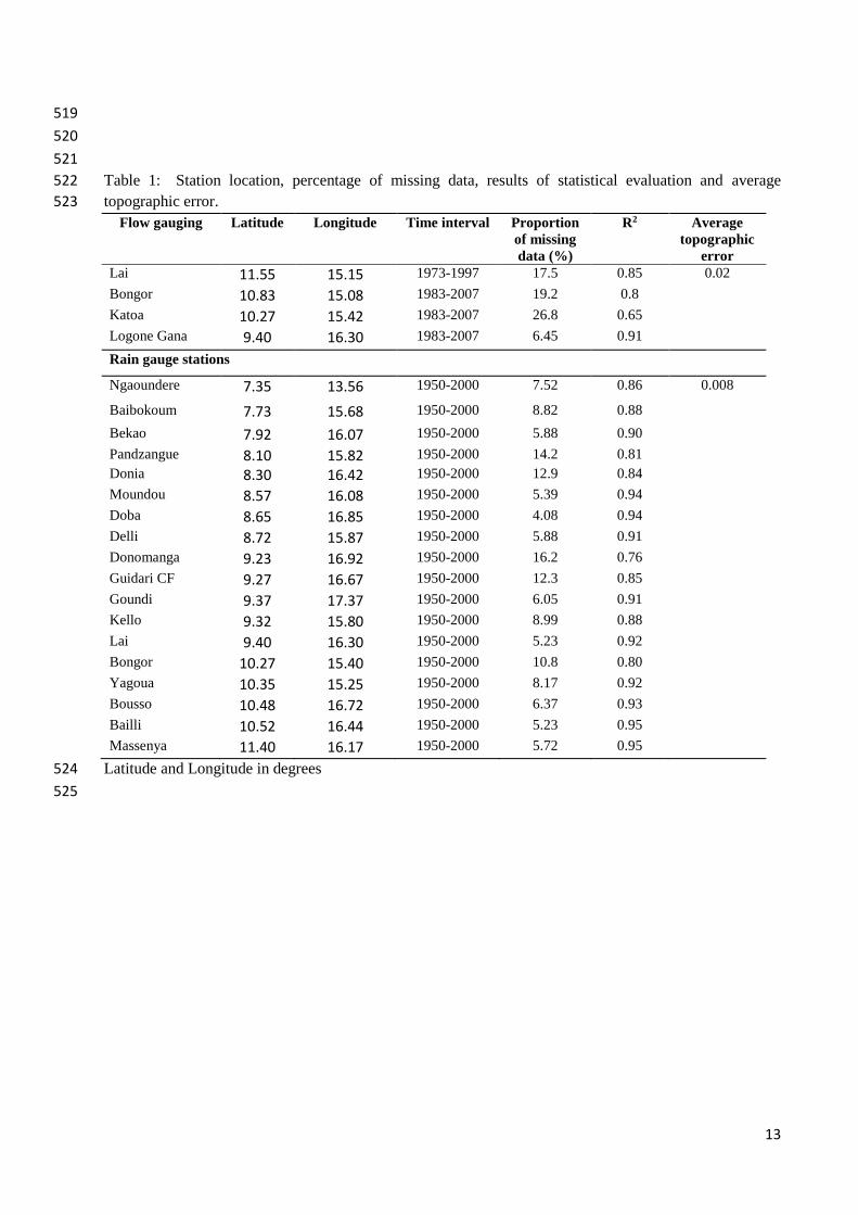
The results indicate that after the second simulation, the model was able to replicate with 293
high accuracy the trends and flow magnitudes (high and low) in the respective seasons as shown 294
in Figures 3 to 6. This justifies the low value of average topographic error 0.02 and the high values 295
of R2. From these results, the newly trained time series were used to infill missing gaps in the 296
different time series in the Logone catchment. The preservation of topology, especially for 297
discharge time series is important because seasonal variation causes high and low flows. The 298
results obtained indicate that this seasonal variation was well preserved across all the gauging 299
stations during the infilling process. In this research more emphasis was put on reducing the 300
topographic error to ensure that the infilled values reflect the seasonal variation of the time series. 301

8
However, a visual observation of flow hydrographs (Figures 3-6) indicate that, the possibility of 302
errors in the original river discharge time series may not be discounted especially for the Bongor 303
station, and this may have a negative impact on the overall performance of the SOM algorithm in 304
this study. 305
The results obtained for rainfall observations were similar to those obtained for discharge 306
with the lowest R2 value of 0.76 and average topographic error of 0.008. Although some authors 307
(Kalteh & Berndtsson, 2007; Mwale et al., 2012) have proposed that to the rainfall time series 308
should be trained together according to spatial location to improve the results, this method was not 309
applied in this study because results obtained were judged to be satisfactory. Of the 18 rainfall 310
stations, 10 had R2 values of 0.90 and above while 7 stations had R2 values of 0.80 and above with 311
only one station (Donomanga) which has the highest percentage of missing observations having a 312
value of 0.76. However, it was noticed that the performance of the model reflected the spatial 313
location of the stations. For example, apart from Bongor CF with a R2 of 0.80, all stations located 314
above 10°N had R2 values above 0.90 while most stations located below this latitude had R2 values 315
between 0.80-0.90. Since the graphs of the all the 18 rain gauge stations cannot be shown, (Figures 316
7 & 8) are used for illustration. Furthermore, it was observed that the SOM algorithm was able to 317
preserve seasonal variation when infilling missing data in rainfall time series just as it did for 318
discharge. 319
The results also indicate that, although this method is quite robust for infilling gaps in 320
hydro-meteorological time series, it cannot be used for infilling gaps in time series with extended 321
periods of missing observations as model performance starts diminishing. This is logical as in such 322
situations the model does not have sufficient data to learn from, thus cannot correctly replicate the 323
pattern in the data. For example time series of measured discharge at Katoa had 1200 consecutive 324
days of missing observations, which represent 13% of the total data entries, produced an R2 of 0.65 325
compared to Logone Gana with 97 consecutive days of missing observations with an R2 of 0.91. 326
This implies that time series with extended periods of missing observations should not be used as 327
the model may infill the missing observations but still fail to replicate the pattern in the data. 328
Although, as shown by Kalteh et al. (2007) and Mwale et al. (2012) this issue can be resolved for 329
rainfall time series by training such time series with data from the same spatial zone, this cannot 330
apply for discharge time series as it is influenced by other catchment characteristics and the river 331
morphology which vary along the river channel. 332
Nevertheless results obtained suggest that SOMs are suitable for infilling gaps in hydro-333
meteorological time series in Sudano-Sahel catchments. Results obtained from this study are 334
comparable to those obtained by Mwale et al. (2012, 2014) in the Lower Shire Floodplain in 335
Malawi, Kang & Yusuf (2012) in the Kelantan and Damansara river basins in Malaysia and Kim 336
et al. (2015) in the Taehwa watershed in Korea 337
The relationship between discharges measured at various stations along the Logone River 338
is shown in Figure 9. The Unified distance matrix (U-matrix) is a graphical display used to illustrate 339
the clustering of the reference vectors in the SOM, it shows the distance between neighbouring 340
map units. The U-matrix can be seen as several component planes which are stacked together one 341
on top of the other. Component planes can either be coloured or grey shaded in a two dimensional 342
lattice. Light colours indicate areas in which the variables are close to each other in the input space, 343
while dark colours illustrate large distances between variables in the input space. Dark colours can 344
be seen as cluster separators while light colours are clusters themselves. Component planes are 345

9
therefore, mostly used for visualizing the correlation between the various variables in the SOM 346
since they can give information concerning the spread of values in each component (Gabrielsson 347
& Gabrielsson, 2006). 348
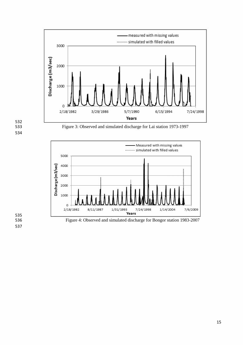
From Figure 9, the relationship between the discharges measured at Bongor, Katoa and 349
Logone Gana is not very discernible. To illustrate that there is no relationship between the 350
discharge time series, Figure 10 shows that the discharges measured at Katoa and Logone Gana 351
gauging stations, which are located downstream of Bongor, are paradoxically lower than discharge 352
measured at Bongor station upstream. This can partly be explained by the fact that during the rainy 353
season when the river overflows its banks, immediately after Bongor station, part of the flow is 354
diverted to fill the Maga dam and part is lost to the floodplains. During the dry season, water is 355
withdrawn from the river without control for various purposes by the inhabitants thus reducing the 356
quantity that eventually reaches Logone Gana station located downstream. This can also be 357
attributed to transmission losses as a result of infiltration to the aquifer through channel bed. Seeber 358
(2013) observed that the discharge recorded at Ndjamena flow gauging station located downstream 359
was lower than that recorded upstream at the Logone Gana station. Candela et al. (2014) reported 360
that a significant proportion of groundwater in the Lake Chad aquifer system was from the Logone 361
River through river and aquifer interactions. 362
363
4) Conclusion 364
The main objective of this study was to use Self-Organizing Maps (SOMs) to infill missing 365
gaps in hydro-meteorological time series in the Logone catchment using data from four river 366
discharge and 18 rain gauge stations riddled with gaps 367
The combination of artificial intelligence and human intelligence (to be able to distinguish 368
the seasonal discharge trends, patterns and magnitudes) greatly improved the overall performance 369
of the SOM algorithm in handling missing data. Other advantages of SOMs include: (i) it does not 370
require input data from neighbouring stations; (ii) unlike other ANN methodologies it does not 371
require extra datasets to train the time series; (iii) it is not computationally intensive; and (iv) it 372
does not require extra storage capacity. 373
Results obtained from this study indicate that, the SOMs algorithm is quite robust for infilling 374
gaps in hydro-meteorological time series, though it is not suitable for infilling gaps in time series 375
with extended periods of missing observations as model performance starts diminishing. This 376
methodology can be used by practitioners to enhance the planning and management of water 377
resources in areas where available records are infested with missing observations. Preservation of 378
topology through a good replication of trends and discharge magnitudes in the time series obtained 379
in this study will reduce the data input uncertainty in our future modelling studies in the catchment. 380
381
Acknowledgements 382
This research was supported by a Commonwealth Scholarship award to the first author. We 383
are grateful to SIEREM and the Lake Chad Basin Commission for providing the data used in this 384
research. 385
386
References 387
Adeloye, A. J., Rustum, R., & Kariyama, I. D. (2012). Neural computing modelling of the reference 388
crop evapotranspiration. Environmental Modelling & Software, 29, 61-63. 389

10
390
Alhoniemi, E., Himberg, J., Parhankangas, J. & Vesanto, J. (2002). SOM Toolbox - Online 391
Documentation. 392
393
ASCE Task Committee on Application of Artificial Neural Networks in Hydrology (2000). 394
Artificial Neural Networks in Hydrology. II: Hydrologic Applications. Journal of Hydrologic 395
Engineering, 5:2(124), 124-137. 396
397
Boyer, J., Dieulin C., Rouche, N., Cres, A., Servat, E, & Paturel, J. (2006). SIEREM: An 398
Environmental Information System for Water Resources, Vol. IAHS Publication 308. IAHS Press: 399
Wallingford, United Kingdom. 400
401
Campozano, L., Sanchez, E., Aviles, A., & Samaniego, E. (2012). Evaluation of infilling methods 402
for time series of daily precipitation and temperature: The case of the Ecuadorian Andes. Maskana, 403
5(1), 99-115. 404
405
Candela, L., Elorza, F. J., Tamoh, K., Jiménez-Martínez, J., & Aureli, A. (2014). Groundwater 406
modelling with limited data sets: the Chari– Logone area (Lake Chad Basin, Chad). Hydrological 407
Processes, 28, 3714-3727. 408
409
Coumou, D. & Rahmstorf, S. (2012). A decade of weather extremes. Nature Climate Change, 2, 410
491-496. 411
412
Daniel, E. B., Camp, J. V., LeBoeuf, E. J., Penrod, J. R., Dobbins, J. P. & Abkowitz, M. D. (2011). 413
Watershed modelling and its applications: A state-of-the-art review. The Open Hydrology 414
Journal, 5, 26-50. 415
416
Dastorani, M. T., Moghadamnia, A., Piri, J. & Ramirez, M. R. (2010). Application of ANN and 417
ANFIS models for reconstructing missing flow data. Environmental Monitoring and Assessment, 418
166(1-4), 421-34. 419
420
Elshorbagy, A. A., Panu, U. S. & Simonovic, S. P. (2000). Group-based estimation of missing 421
hydrological data: Approach and general methodology. Hydrological Sciences Journal, 45(6), 422
849-866. 423
424
Gabrielsson, S., & Gabrielsson, S. (2006). The use of Self-Organizing Maps in Recommender 425
Systems: A survey of the Recommender Systems field and a presentation of a State of the Art 426
Highly Interactive Visual Movie Recommender System. Master Thesis, Uppsala University. 427
428
Garcia, H., & Gonzalez, L. (2004). Self-organizing map and clustering for wastewater treatment 429
monitoring. Engineering Applications of Artificial Intelligence. 17(3), 215–225. 430
431

11
Harvey, C. L., Dixon, H. & Hannaford, F. (2012). An appraisal of the performance of data-infilling 432
methods for application to daily mean river flow records in the UK. Hydrology Research, 433
43(5) 618-636. DOI: 10.2166/nh.2012.110. 434
435
Ismail, S., Shabri, A., & Samsudin, R. A. (2012). Hybrid model of self-organizing maps and least 436
square support vector machine for river flow forecasting. Hydrology and Earth System Sciences, 437
16, 4417-4433. 438
439
Kagoda, P. A., Ndiritu, J., Ntuli, C., & Mwaka, B. (2010). Application of radial basis function 440
neural networks to short-term streamflow forecasting, Physics and Chemistry of the Earth, 35, 571-441
581. 442
443
Kalteh, A. M. & Hjorth, P. (2009). Imputation of missing values in a precipitation–runoff process 444
database. Hydrology Research, 40(4), 420-432. 445
446
Kalteh A. M., Hjorth, P., & Berndtsson R. (2008). Review of the self-organizing map (SOM) 447
approach in water resources: Analysis, modelling and application. Environmental Modelling & 448
Software, 23, 835, – 845. 449
450
Kalteh, A. M., & Berndtsson, R. (2007). Interpolating monthly precipitation by self-organizing 451
map (SOM) and multilayer perceptron (MLP), Hydrological Sciences Journal, 2(2), 305-317. 452
453
Kang, H. M., & Yusof, F. (2012). Application of Self-Organizing Map (SOM) in Missing Daily 454
Rainfall Data in Malaysia. International Journal of Computer Applications, 48(5). 455
456
Kashani, M. H., & Dinpashoh, Y. (2012). Evaluation of efficiency of different estimation methods 457
for missing climatological data. Stochastic Environmental Research and Risk Assessment, 26, 59–458
71. 459
460
Kim, M., Baek, S., Ligaray, M., Pyo, J., Park, M., & Cho, K. H. (2015). Comparative Studies of 461
Different Imputation Methods for Recovering Streamflow Observation. Water, 7, 6847–6860. 462
463
Kingston, G. B., Dandy, G. C. & Maier, H. R. (2008a). AI Techniques for Hydrological Modelling 464
and Water Resources Management. Part 2 - Optimization, in L. N. Robinson (editor). Water 465
Resources Research Progress, Nova Science Publishers, pp. 67-99. 466
467
Kingston, G. B., Dandy, G. C., & Maier, H. R. (2008b). AI Techniques for Hydrological Modelling 468
and Water Resources Management. Part 1 - Simulation, in L. N. Robinson (editor). Water 469
Resources Research Progress, Nova Science Publishers, pp. 15-65. 470
471
Kohonen, T. Self-Organizing Maps, Springer Series in Information Sciences, vol. 30, Springer, 472
Heidelberg, 1st ed., 1995; 2nd ed., 1997. 473
474

12
Mwale, F. D., Adeloye A. J., & Rustum R. (2014). Application of self-organising maps and multi-475
layer perceptron-artificial neural networks for streamflow and water level forecasting in data-poor 476
catchments: the case of the Lower Shire floodplain, Malawi. Hydrology Research, 45(6), 838-854. 477
478
Mwale, F. D., Adeloye, A. J., & Rustum R. (2012). Infilling of missing rainfall and streamflow 479
data in the Shire River basin, Malawi – A self-organizing map approach. Physics and Chemistry 480
of the Earth, 50-52, 34-43. 481
482
Ng, W. W., & Panu, U. S. (2010). Infilling missing daily precipitation data at multiple sites using 483
the multivariate truncated normal distribution model for weather generation. Water, 8 pp. 484
485
Presti, R. L., Barca, E. & Passarella, G. A. (2010). Methodology for treating missing data applied 486
to daily rainfall data in the Candelaro River Basin (Italy). Environmental Monitoring and 487
Assessment, 160, 1-22. 488
489
Rustum, R., & Adeloye, A. J. (2007). Replacing Outliers and Missing Values from Activated 490
Sludge Data Using Kohonen Self-Organizing Map. Journal of Environmental Engineering, 133(9), 491
909-916. 492
493
Seeber, K. (2013). Consultation of the Lake Chad Basin Commission on Groundwater 494
Management. Project: Sustainable Management of the Lake Chad Basin, BGR No:05-2355. 495
496
Vesantu, J., Himberg, J., Alhoniemi, E & Parhankangas, J. (2000). SOM Toolbox for Matlab 5. 497
Report A57. Helsinki University of Technology, Helsinki, Finland. 498
499
WWAP (United Nations World Water Assessment Programme). 2015. The United Nations World 500
Water Development Report 2015: Water for a Sustainable World. Paris, UNESCO 501
502
503
504
505
506
507
508
509
510
511
512
513
514
515
516
517
518
13
519
520
521
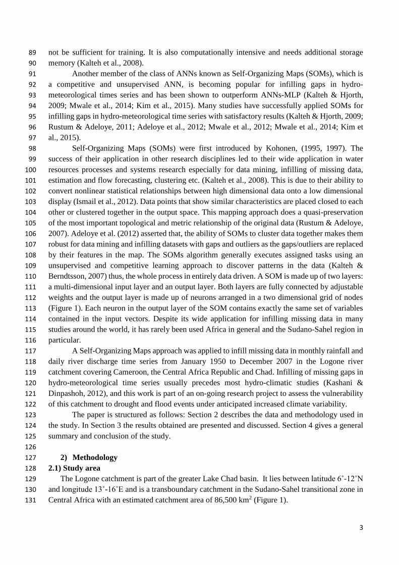
Table 1: Station location, percentage of missing data, results of statistical evaluation and average 522
topographic error. 523
Flow gauging Latitude Longitude Time interval Proportion of missing data (%)
R2 Average topographic
error Lai 11.55 15.15 1973-1997 17.5 0.85 0.02
Bongor 10.83 15.08 1983-2007 19.2 0.8
Katoa 10.27 15.42 1983-2007 26.8 0.65
Logone Gana 9.40 16.30 1983-2007 6.45 0.91
Rain gauge stations
Ngaoundere 7.35 13.56 1950-2000 7.52 0.86 0.008
Baibokoum 7.73 15.68 1950-2000 8.82 0.88
Bekao 7.92 16.07 1950-2000 5.88 0.90
Pandzangue 8.10 15.82 1950-2000 14.2 0.81 Donia 8.30 16.42 1950-2000 12.9 0.84
Moundou 8.57 16.08 1950-2000 5.39 0.94
Doba 8.65 16.85 1950-2000 4.08 0.94
Delli 8.72 15.87 1950-2000 5.88 0.91
Donomanga 9.23 16.92 1950-2000 16.2 0.76
Guidari CF 9.27 16.67 1950-2000 12.3 0.85
Goundi 9.37 17.37 1950-2000 6.05 0.91
Kello 9.32 15.80 1950-2000 8.99 0.88
Lai 9.40 16.30 1950-2000 5.23 0.92
Bongor 10.27 15.40 1950-2000 10.8 0.80
Yagoua 10.35 15.25 1950-2000 8.17 0.92
Bousso 10.48 16.72 1950-2000 6.37 0.93
Bailli 10.52 16.44 1950-2000 5.23 0.95
Massenya 11.40 16.17 1950-2000 5.72 0.95
Latitude and Longitude in degrees 524
525

14
526
Figure 1: Architecture of an SOM (Adapted from Kagoda et al., 2010) 527
528
529
Figure 2: Map of study area showing rain and flow gauging stations 530
531
15
532
Figure 3: Observed and simulated discharge for Lai station 1973-1997 533
534
535
Figure 4: Observed and simulated discharge for Bongor station 1983-2007 536
537

16
538
Figure 5: Observed and simulated discharge for Katoa station 1983-2007 539
540
541
Figure 6: Observed and simulated discharge for Logone Gana station 1983-2007 542
543
544
Figure 7: Observed and simulated rainfall for Ngaoundere (1950-1960) 545

17
546
547
Figure 8: Observed and simulated rainfall for Kello (1990-2000) 548
549
550
Figure 9: Component planes for discharge at all the stations 551
18
552
Figure 10: Discharge at Bongor, Katoa and Logone Gana 1983-2007 553
554