e.

USING CORIOLIS FORCE TO FACILITATE MOLECULAR

TRANSPORTATION AND FLUID MIXING IN CD MICROFLUIDICS

PLATFORM

_______________

A Thesis

Presented to the

Faculty of

San Diego State University

_______________

In Partial Fulfillment

of the Requirements for the Degree

Master of Science

in

Aerospace Engineering

_______________

by

Dhruv Bharatkumar Patel

Fall 2012

iii

Copyright © 2012

by

Dhruv Bharatkumar Patel

All Rights Reserved

iv

DEDICATION

This Thesis is dedicated to my Mom and Dad.

v

ABSTRACT OF THE THESIS

Using Coriolis Force to Facilitate Molecular Transportation and Fluid Mixing in CD Microfluidics Platform

by Dhruv Bharatkumar Patel

Master of Science in Aerospace Engineering San Diego State University, 2012

This study investigates the influence of Coriolis force on transport and hybridization of DNA molecules and Fluid mixing in compact disk (CD) microfluidic platform where centrifugal force is used as the driving force. While the effect of Coriolis force on fluid flow in CD microfluidic channels has been studied experimentally and numerically only recently, its influence on DNA molecule migration and hybridization and on fluid mixing has not been investigated so far. This study addresses this phenomenon through numerical simulation and demonstrates that for most practical geometrical configurations and angular velocity ranges reported in the literature, the Coriolis force introduces significant qualitative and quantitative spatial variations in the hybridization of DNA molecules, particularly at locations near the periphery. In a particular example investigated here, hybridization was observed to reach steady-state at some locations in about half the time required in the absence of Coriolis force. However, our results further indicate that the time frame for hybridization is so fast (< 1 sec) that the effect due to Coriolis force on the location of hybridization is more important than time of hybridization. Our results indicate that for low viscosity fluids, angular velocities as low as 25 rad/sec could introduce Coriolis force that is as high as at least 25% of the main driving centrifugal force. As for the fluid mixing under microchannel with and without obstacles significant amount of fluid mixing efficiency is observed for both kind of channel, the results demonstrates that at higher omega for channel with obstacle has more mixing efficiency then without obstacles.

vi

TABLE OF CONTENTS

PAGE

ABSTRACT ...............................................................................................................................v

LIST OF TABLES .................................................................................................................. vii

LIST OF FIGURES ............................................................................................................... viii

ACKNOWLEDGEMENTS .......................................................................................................x

CHAPTER

1 INTRODUCTION .........................................................................................................1

1.1 What is Microfluidics? .......................................................................................1

1.2 Basic Principle of Microfluidics ........................................................................2

1.3 Modeling Diffusion ............................................................................................2

1.4 CD Microfluidics ...............................................................................................4

1.5 Coriolis Effect ....................................................................................................6

2 LITERATURE SURVEY ..............................................................................................7

3 MULTIPHYSICS MODEL DEVELOPMENT ...........................................................12

3.1 Fluid Dynamics System ...................................................................................13

3.2 Migration of DNA Molecules ..........................................................................13

3.3 DNA Hybridization Kinetics ...........................................................................13

4 SOLUTION OF NUMERICAL MODEL ...................................................................17

5 NUMERICAL RESULTS AND DISCUSSION FOR MOLECULAR TRANSPORTATION ..................................................................................................20

6 NUMERICAL RESULTS AND DISCUSSION FOR FLUID MIXING ....................29

6.1 Velocity Distribution in Microchannel ............................................................31

6.2 Concentration Plots ..........................................................................................31

6.3 Mixing Efficiency ............................................................................................35

7 CONCLUSION ............................................................................................................38

BIBLIOGRAPHY ....................................................................................................................40

APPENDIX

MESHED GEMETRY FOR STRAIGHT CHANNELS .............................................43

vii

LIST OF TABLES

PAGE

Table 2.1. Summary of Recent Results in Flow Rate and Velocity in CD Microfluidic Platform Reported in the Literature .............................................................................10

Table 4.1. Summary of the Boundary Conditions and Constants Used in the Numerical Model for DNA Hybridization in Straight Channel ...................................19

Table 5.1 Summary of the Effect of Angular Velocity on the Coriolis Force Induced Velocity Pattern. Width = 360µm ................................................................................21

Table 6.1. Summary of the Boundary Conditions and Constants Used in the Numerical Model for Fluid Mixing in Straight Channel .............................................31

Table 6.2. Velocity Distributions for Different Omega ...........................................................32

Table 6.3. Rate of Change of Concentration with Time ..........................................................33

viii

LIST OF FIGURES

PAGE

Figure 1.1. Size characterizations of microfluidics devices. .....................................................1

Figure 1.2. Parabolic velocity profile in microchannel. .............................................................3

Figure 1.3. Velocity profile in open channel through electro-osmotic pumping. ......................3

Figure 1.4. Velocity profile in closed channel through electro-osmotic pumping. ...................4

Figure 1.5. Schematic of the CD based microchannel. ..............................................................5

Figure 1.6. Coriolis force on the earth surface...........................................................................6

Figure 2.1. Typical configuration of a CD microfluidic platform. r - radius, ω - angular velocity, u – velocity. FCorilois represents Coriolis force while the centrifugal force is represented as FCen. .........................................................................8

Figure 2.2. The ratio of Coriolis to centrifugal force for various widths of channel (FCoriolis/FCentrifugal = ρb2ω/4). For a case of ν= 1e-3 Pa-s and ρ = 1000Kg/m3, FCoriolis/FCentrifugal = 2.5e5 b2ω. .........................................................................................9

Figure 2.3. Effect of width and angular velocity on the dominance of Coriolis force. .............9

Figure 3.1. DNA hybridization model. ....................................................................................15

Figure 3.2. Cylindrical co-ordinate system. .............................................................................16

Figure 4.1. Illustration of a typical micro channel in a CD microfluidic platform. .................18

Figure 5.1. Effect of angular velocity on the Coriolis force and the ratio of the maximum velocity to the mean velocity of flow. ........................................................21

Figure 5.2. Geometry of a microchannel in a CD platform considered in this study. There are five hybridization sites of 360 µm width and 500 µm length along the length of the channel. These probe sites are placed at a spacing of 1 mm (clear span). L = 10.1 mm length and 360µm width and 125µm depth. .....................23

Figure 5.3. (a) Transient variation of hybridized DNA (dsDNA) at various locations in microchannel under ω = 100 rad/sec., (b) effect of angular velocity on transient variation of hybridized DNA (dsDNA) at various locations in microchannel, and (c) effect of angular velocity on transient variation of hybridized DNA (dsDNA) at various locations in microchannel for ω = 100 rad/sec and ω = 25 rad/sec for non-specific and specific hybridization. .....................24

Figure 5.4. (a) Effect of channel width on transient variation of hybridized DNA (dsDNA) at various locations in microchannel, and (b) effect of channel width on transient variation of hybridized DNA (dsDNA) at Point 'C" for ω = 50 rad/sec for non-specific and specific hybridization. ....................................................27

ix

Figure 5.5. Accumulation ratios at the different capture probe locations as a function of the angular velocity. ................................................................................................28

Figure 6.1. Microchannel without obstacles. ...........................................................................30

Figure 6.2. Microchannel with obstacles. ................................................................................30

Figure 6.3. Change of concentration at different angular velocity for microchannel without obstacles. .........................................................................................................34

Figure 6.4. Change of concentration at different angular velocity for microchannel with obstacles. ..............................................................................................................34

Figure 6.5. Mixing efficiency of microchannel without obstacles. .........................................35

Figure 6.6. Mixing efficiency of microchannel with obstacles. ..............................................36

Figure 6.7. Mixing efficiency plot of microchannel without obstacles. ..................................36

Figure 6.8. Mixing efficiency plot of microchannel with obstacles. .......................................37

Figure A.1. Straight channel ~10mm length. ...........................................................................44

Figure A.2. Straight channel ~5mm length. .............................................................................45

Figure A.3. Straight channel with obstacles. ...........................................................................46

x

ACKNOWLEDGEMENTS

I would like to acknowledge my heartily thanks for this thesis work to my advisor Dr.

Sam Kassegne, who has shown support throughout my research work and helped me

understand the basic knowledge of engineering.

I would also like to thanks my other professor Dr. Satchi Venkataraman and Dr.

Luciano Demasi for being there for me when I needed them the most.

I also thank my Lab mates and friends for helping me to understand the things

especially which were related to bioengineering.

1

CHAPTER 1

INTRODUCTION

1.1 WHAT IS MICROFLUIDICS? Microelectronics was the most significant enabling technology of the last century.

With integrated circuits and progress in information, microelectronic has changed the way

we work,discover and invent. From its inception through late 1990’s miniaturization in

microelectronics followed Moore’s Law doubling the integration density every 18 months.

Presently poised at the limit of photolithography technology this pace will slow down to

doubling integration density every 24 months.

In late 1970s the silicon technology was extended to machining mechanical

microdevices, which later came to know as MEMS (Microelectronics and Mechanical

System). With fluidics and optical in microdevices, Microsystem Technology (MST) is a

more accurate description. The Development of microflow sensor, micropumps and

microvalves in early 1980s dominated the early stages of microfluidics. Several competing

term such as ‘Microfluidics’, ‘MEMS- fluidics’, ‘Bio- MEMS’ appeared for the research

discipline which was dealing with the transport phenomena and fluid devices at microscopic

level. (See Figure 1.1 [28]).

Figure 1.1. Size characterizations of microfluidics devices. Source: Nguyen, Nam-Trung, and Steven. T. Wereley. Fundamentals and Application of Microfluidics. Boston: Artech House, 2002.

2

Microfluidics Devices need not to be silicon-based fabricated using silicon based

machining technology. The main advantage of the microfluidics is to use scaling law for

better performance and this can be derived by microscopic amount of fluid which a

microfluidics device can handle. Regardless of the material and instrument used for

machining the micro-device only the part where fluid is processed need to be miniaturized.

Handling the fluid is the main key aspect of the microfluidics, miniaturizing the

whole system is often beneficial but is not a requirement of the microfluidics devices. The

term microfluidics does not necessarily means its fluid mechanics system but it rather refers

to as the small scale causing change in the fluid behavior [28].

1.2 BASIC PRINCIPLE OF MICROFLUIDICS There are two common methods by which fluid actuation through microchannel can

be achieved:

a. Pressure Driven Flow: In pressure driven flow, in which the fluid is pumped through the device via positive displacement pumps, such as syringe pumps. One of the basic laws of fluid mechanics for pressure driven laminar flow, the so-called no-slip boundary condition, states that the fluid velocity at the walls must be zero. This produces parabolic velocity profile within the channel [33] (as shown in Figure 1.2 [33]).

The parabolic velocity profile has significant implications for the distribution of molecules transported within a channel. Pressure driven flow can be a relative inexpensive and quite reproducible approach to pumping fluids through microdevices [33].

b. Electrokinetic Flow: Another common method for transferring fluid in microchannel is through electro-osmotic pumping in open microchannel. In such channel if the walls of the channel as the electric charge as most surface do then on applying the electric field the ion moves towards the electrodes of the opposite polarity in the open channel. This will create the motion of the fluid via viscous force into convective motion of the fluid in the channel; if the channel is open the velocity profile remains uniform along the width of the channel [33]. (See Figure 1.3 [33]).

If the channel is closed or back pressure exist in the channel the recirculation will appear in the channel causing the velocity profile at the center of the channel to move on the opposite direction to that of the flow [33]. (See Figure 1.4 [33]).

1.3 MODELING DIFFUSION The diffusion process can be described as in terms of Fick’s first law and second law:

a. Fick’s First Law: Fick’s postulated that diffusion in one direction, the flow; J of a substance through a plane perpendicular to the direction of the diffusion is directly

3

Figure 1.2. Parabolic velocity profile in microchannel. Source: Schilling, Eric. “Basic Microfluidic Concepts.” September 7, 2001. http://faculty.washington. edu/yagerp/microfluidicstutorial/basicconcepts/basicconcepts.htm.

Figure 1.3. Velocity profile in open channel through electro-osmotic pumping. Source: Schilling, Eric. “Basic Microfluidic Concepts.” September 7, 2001. http://faculty. washington.edu/yagerp/microfluidicstutorial/basicconcepts/basicconcepts.htm.

4

Figure 1.4. Velocity profile in closed channel through electro-osmotic pumping. Source: Schilling, Eric. “Basic Microfluidic Concepts.” September 7, 2001. http://faculty.washington.edu/yagerp/microfluidicstutorial/basicconcepts/basicconcepts.htm.

proportional to the rate of change of concentration with distance , the concentration gradient and the equation is given as follows;

J = -D (1.1)

Where; J is the flux (the rate of mass flow rate per unit area in direction x in g mol/cm2 /s), D is the diffusion coefficient in cm2/s and C is the concentration of the solute in g mol/cm3 [1].

b. Fick’s Second Law: For solving most of the diffusion cases the first law is insufficient because usually the diffusion value is unknown, and this can be better handled by the Fick’s second law, given as;

= D (1.2)

Where; C is the concentration and t is the time.

According to the equation the time rate of change of concentration is equal to the spatial rate of change of direction of the concentration gradient. When both flow and diffusion occurs the time rate of change of concentration can be given as following equation;

= D = -v (1.3)

Where, v is the velocity of the flow in x direction [1].

1.4 CD MICROFLUIDICS Microflow can be actuated by rotational (Centrifugal and Coriolis force) forces by

spinning the microfluidic network on the Compact Disk. Such type of flow actuation is

known as CD Microfluidics. CD Microfluidics has gained considerable attention owing to

5

biomedical application. Its prime advantages lies in handling large varieties of sample liquid,

ability to gate the flow of the liquid, simple rotational motor requirement and large range of

the flow rates can be attained. For low rotational speed (ignoring Coriolis force) the

governing equation for the rotating frame can be described by using the pressure gradient [6].

(1.4)

Where; is angular velocity of rotation and x is the distance from the center of the rotation,

although the force is function of radial coordinate, the flow attains the fully developed

condition and the parabolic velocity profile is attained. The discharge rate (Q) is obtained by

integrating velocity profile over the cross-section area (A) [6].

(1.5)

Where, Dh is the hydraulic diameter of the channel, is the distance from the center

of the CD, is the radial extent of the fluid, L is the length of the liquid in the liquid

channel, is the density of the liquid and is the dynamic viscosity of the liquid [6]. (See

Figure 1.5 [6]).

Figure 1.5. Schematic of the CD based microchannel. Source: Chakraborty, Suman, ed. Microfluidics and Microfabrications. New York: Springer, 2010.

6

1.5 CORIOLIS EFFECT Coriolis force is felt by an observer who is on rotating frame of reference and moves

inward or outward from its position or axis. It acts perpendicular to the motion of the

observer or to that of rotating axis. In vector notation the Coriolis force can be determined as

(1.6)

If body on the earth moves northern hemisphere then due to Coriolis force it drives

toward the east and for southern hemisphere to moves toward west. The reason for the

contrary deflection is the body moving towards the north always falls ahead of the earth

circumferential velocity and body travelling towards the south fall behind the earth

circumferential velocity [2]. (See Figure 1.6 [2]).

Figure 1.6. Coriolis force on the earth surface. Source: Benenson, Walter, John. W. Harris, Horst Stocker, and Holger Lutz, eds. Handbook of Physics. New York: Springer, 2002.

7

CHAPTER 2

LITERATURE SURVEY

Over the past several years, research and commercial development interest in CD

microfluidic platforms has experienced a significant increase [13, 20, 24, 25, 27, 34]. Further,

there has been a noticeable expansion of the reported application of such platforms to new

areas such as complete sample-to-answer systems in molecular clinical diagnostics, blood

separation, gene sequencing and gene profiling systems [20, 23, 26, 32]. The most important

driving force for this increased interest in the platform is the absence of moving parts that

simplify fabrication as well as operation of devices. The physics of fluid flow in such

platforms through centrifugal force that provides the driving pressure gradient has been

studied extensively through experiments and numerical models by several researchers [20,

24, 34]. However, it was only recently that the effect of Coriolis force on fluid flow was

demonstrated and quantitatively determined by Brenner, Zengerle, and Ducrée [5] and

Ducrée et al. [12] who used a rotating frame of reference for a CD platform rotated by an

angular velocity. The work of Brenner, Zengerle, and Ducrée [5] as well as Ducrée et al. [12]

showed that Coriolis force introduces a significant change in fluid velocity which is

conveniently adopted as a fluid flow switch [5] and mixer [12].

Figure 2.1 illustrates typical geometry parameters and forces acting on a CD

microfluidic platform. Centrifugal force creates an artificial gravity - and hence a pressure

gradient - pointing in the radial direction of the channels. This force scales with the square of

the frequency of the angular velocity at which the channel is rotated. Coriolis force, on the

other hand, is induced when the resulting fluid flow is observed from a rotating non-inertial

reference frame. This apparent force acts perpendicular to the plane of the flow channel and

the angular velocity. As a result, the fluid experiences pumping in a radial direction due to

centrifugal force but its direction and magnitude are further modified by the radial and

tangential components of Coriolis force. As will be shown later in section 2, Coriolis force

depends linearly on the angular velocity (ω) and varies with the square of the channel width.

For a fluid of dynamic viscosity ‘η’ and density ‘ρ’ flowing in a channel of width ‘b’ on a

8

Figure 2.1. Typical configuration of a CD microfluidic platform. r - radius, ω - angular velocity, u – velocity. FCorilois represents Coriolis force while the centrifugal force is represented as FCen.

CD platform rotating at angular velocity of 'ω', it can be shown that the ratio of Coriolis force

to centrifugal force can be approximated as FCoriolis/FCentrifugal = ρb2ω/4h [12].

This ratio is an important indicator of the potential effect Coriolis force has on fluid

flow in a CD platform (see Figure 2.2 [12]). Figure 2.3 presents a family of curves

corresponding to different angular velocities demonstrating the effect of channel width on

Coriolis force. Figure 2.2 [12] demonstrates that even at lower angular velocities in the range

of 25 rad/sec, Coriolis force could be significant (25% of the centrifugal force) if the channel

widths are moderately wide (in the range of 200 microns).

To provide a perspective to the range of dimensions used in recently published works

in CD microfluidic platforms, Table 2.1 summarizes some of the typical CD microchannel

configurations reported along with angular velocities. The width of channels varies from

20µm [4] to 500µm [22, 25] whereas the depth of channels varies from 34µm [27] to

1000µm [31]. The variation of lengths is from 8.4mm [10] to 21 mm [4, 11]. Angular

velocity variations from 40 rad/sec (~400 rpm) [25] to 950 rad/sec (9500 rpm) [10] have

been reported. Table 2.1 suggests that the variations in dimensions of microchannels,

particularly width and depth, used by different researchers are in the order of 25 times or

more. This, in turn, translates to substantial variations in fluid velocities. Figure 2.2 plots

these results reported in the literature on a graph of angular velocity vs. width and depicts

which results fall in a region where Coriolis force exceeds the driving centrifugal force (i.e.

region A). Ranges where the Coriolis force is more than 50% and 25% of the main driving

FCoriolis = 2ρωu

FCentrifugal = ρω2r

Z

Y X

9

Figure 2.2. The ratio of Coriolis to centrifugal force for various widths of channel (FCoriolis/FCentrifugal = ρb2ω/4). For a case of ν= 1e-3 Pa-s and ρ = 1000Kg/m3, FCoriolis/FCentrifugal = 2.5e5 b2ω. Source: Ducrée, Jens, Thilo Brener, Thomas Glatzel, and Roland Zengerle. “Coriolis-Induced Switching and Mixing of Laminar Flows in Rotating Microchannels.” Paper presented at the Proceedings of Micro Technology, Munich, Germany, October 2003.

Figure 2.3. Effect of width and angular velocity on the dominance of Coriolis force.

10

Table 2.1. Summary of Recent Results in Flow Rate and Velocity in CD Microfluidic Platform Reported in the Literature Authors Width

(µm) Depth (µm)

Length (mm)

Ang. Velocity (rpm)

Ang. Velocity (ω) – rad/sec

Madou et al. [27] 150 34 -- 524 – 1126 50 -100

Madou et al. [25] 20-500 16-340 -- 400-1600 40-160

Kim et al. [23] 50 40 --- 500 50

Brenner, Zengerle, and Ducrée [5]

360 125 10.1 3500 350

Ducree et al. [12] --- --- --- 1000 100

Kim et al. [22] 500 50, 18 or 8 15 --- fixed velocity of 0.67 mm/s

Kim et al. [21] 215 80 13 --- 80

Riegger et al. [31] 30 1000 10 6300 – 9500 630-950

Ducrée et al. [10] 250 150 8.4 3000 300

Brenner, Zengerle, and Ducrée [5]

360 125 10.1 750 and 3500 75 and 350

Ducree et al. [11] 320 65 21 3000 300

Zhang et al. [35] 60 40 2.5 1550 155

Riegger et al. [30] --- 400,800 25 6000 600

Jia et al. [17] 200-1000 25-250 25 300-700 30-70

Haeberle et al. [15] 300 85 32 2500 250

Brenner et al. [3] 300 25 50 10000 1000

Cho et al. [7] 127-762 60-800 60 600-1500 60-150

11

force of centrifugal force are indicated as region B and C, respectively. It is instructive to

note that a significant number of results reported in the literature fall in regions A, B, and C

suggesting that their corresponding Coriolis forces are 25% - 100% of the centrifugal force.

As this CD fluidics platform is finding increasing research and commercial interests

in molecular clinical diagnostics, an accurate understanding of the hybridization of single-

stranded DNA molecules (ssDNA) as affected by all the body forces acting on the fluid

medium such as Coriolis force becomes more important. There are currently several research

publications that model the hybridization of ssDNA molecules in microarray format [8, 9, 19,

22]. However, research in the modeling of DNA hybridization phenomenon in CD

microfluidic platform is extremely rare.

Further, to the best of our knowledge, the influence of Coriolis force on the migration

and hybridization phenomenon of DNA molecules, particularly on the distribution of

hybridization region, has not been reported in the literature yet. In this paper, therefore, we

present a numerical model for the transport and hybridization of DNA in CD microfluidic

platform. We demonstrate that as the angular rotation of the CD platform increases, the rate

of hybridization experiences a qualitative as well as a quantitative change resulting in

increased hybridization at the peripheries. This has implications in the design of the location

of the probes as well as the detection system. The paper is arranged in the following fashion:

section 1 presents introduction; section 2 presents the numerical model development; section

3 covers the solution of the developed model; section 4 presents numerical results and their

discussion followed by section 5 which presents experimental results and section 6 which

outlines concluding remarks.

Results reported in the literature are indicated in Figure 2.3 with their position on the

graph corresponding to their respective angular velocity and channel width. Three different

scenarios corresponding to cut-off values of 25, 50, and 100% are considered for

FCoriolis/FCentrifugal ratio to demonstrate where Coriolis force is significant enough to affect flow

patterns in published results. Region C represents the range where Coriolis force is between

25%-50% of centrifugal force. Region B indicates the ranges where the Coriolis force is

between 50% and 100% of centrifugal force, while Region A represents the region where the

Coriolis force is more than 100% of centrifugal force.

12

CHAPTER 3

MULTIPHYSICS MODEL DEVELOPMENT

The modeling of migration and hybridization of single-stranded DNA molecules in

CD microfluidic platform requires the consideration of multi-physics phenomenon. To

illustrate our discussion, we consider a generic CD microfluidic platform shown in Figure

1.1.

The first physics is that of fluid flow that is described by the continuity equations and

Navier-Stokes equation for incompressible flow (Eq. 3.1.a-b). However, the body force term

in the conventional Navier-Stokes equation includes the centrifugal as well as the Coriolis

forces as shown in Eq. 3.1.c and 3.1.d. The second physics involves the advective transport

of DNA molecules through microchannels as described by Nernst-Planck equation (Eq. 3.2).

The transport is enabled by Brownian diffusion and convective fluid flow. The third set of

equations consists of hybridization model for ssDNA (single-stranded DNA) that in turn

includes equilibrium equation of DNA association and dissociation and the transient first-

order heterogeneous hybridization reaction rate equation (Eq. 3.1.a – b). To keep track of the

concentration of hybridized double-stranded DNA (dsDNA) that accumulates on the capture

surfaces, a diffusion-only model is added (Eq. 3.1.c) [18].

For clarity, the physics and chemical equilibrium reactions considered in this study

are grouped below under three classifications, namely, (i) fluid dynamic system, (ii) DNA

migration physics, and (iii) DNA hybridization physics. Taken together, these equations

developed below describe DNA molecule transport and hybridization processes that occur in

CD microfluidic platforms under the combined effects of centrifugal and Coriolis forces. The

model assumes 3-dimensional formulations as the capture probes in typical hybridization

channels are placed on the bottom floor of the channel in a 2-dimensional plane with fluid

flow passing over them in a 3-D fashion. Further, assumptions of 2-dimension are invalid as

the Coriolis force is a function of two of the planar coordinates only whereas the fluid flow is

3-dimensional. Note that Coriolis force exists only in the plane of angular rotation. Here, as

13

can be seen clearly from Eqs. (3.1.c) and (3.1.d), centrifugal force scales with the square of

the angular velocity while Coriolis force is a linear function of the angular velocity.

3.1 FLUID DYNAMICS SYSTEM The Navier–Stoke’s equations which are defined here to include the continuity

equation and equation of momentum conservation are given as

0. =∇ U (Continuity Equation) (3.1.a)

(Momentum Equation) (3.1.b)

Centrifugal and Coriolis forces given by )( r×× ϖϖρ and U×ϖρ

2 , respectively, from

the total body forces on the bulk fluid, these forces can further be broken down to their x-, y-,

and z-components.

(3.1.c)

(3.1.d)

(3.1.e)

Where,

p – fluid pressure, t – time, U – velocity field, μ- viscosity, ρ – density of fluid, u – velocity

in the x-direction, v – velocity in the y-direction, and ω= angular velocity in the x-y plane.

3.2 MIGRATION OF DNA MOLECULES The movement of ssDNA molecules in the domain is governed by convective-

diffusive transport equation that accounts for diffusion and convection and is given as:

DNADNA

DNA cuRcDt

cDNA ∇⋅−=∇−•∇+

∂

∂)( (Nernst-Planck Equation) (3.2)

Where CDNA is concentration of ssDNA molecules in the microarray and DDNA is

diffusion rate of DNA molecules. R is reaction term representing ssDNA species generated in

the domain due to reaction (it is zero in this case).

3.3 DNA HYBRIDIZATION KINETICS DNA hybridization kinetics:

a. The Non-specific Hybridization (also known as Non-specific binding or Non-specific absorption) takes place between the low affinity target and probe which does not have exact complementary sequence and this can lead to false signal on DNA array. But

14

still this non-specific absorption is very important as far as numerical modeling is concerned because DNA hybridization on the probe sites will be combination of specific and non–specific hybridization (Eq. 3.3.b and Eq. 3.3.c) (see Figure 3.1 [14]).

b. Hybridization of ssDNA Molecules: The binding of oligonucleotides (DNA, in our case) is governed by a chemical equilibrium reaction equation. The rate of this hybridization reaction is a function of all the concentrations of all species present in the overall chemical reaction at any given time and is given by the rate law (Eq. 3.3.a) [14]. Target ssDNA molecules from the sample immediately above the capture probe elements may hybridize with the immobilized DNA molecule directly [22] or may first be adsorbed onto the solid surface followed by diffusion over the surface and hybridization [14]. Taking into account only the direct DNA hybridization, the DNA heterogeneous hybridization reaction can be described by considering the chemical reaction given by Eq. 3.3.a. In this equation, the symbol CDNA,Probes represents single stranded DNA molecules immobilized on the solid surface that are available for hybridization (Figure 1.4). The target DNA molecules in the sample above the capture probes (represented by CDNA) bind specifically to the DNA capture probes and form hybridized double-stranded DNA molecules (whose concentration is represented by CDNA, Hybridized) on the surface of the capture elements [19].

HybridizedDNAK

K

DNAobesDNA cccDNAb

DNAa

,Pr, ,

,

← →+

(3.3.a)

Where Ka,DNA is the forward reaction rate constant which governs the hybridization reaction rate and Kb,DNA is the reverse reaction rate constant that determines the disassociation reaction rate.

The temporal variation of the concentration of hybridized double-stranded DNA molecules is given by a transient first-order reaction rate equation as shown below:

(3.3.b)

The term CDNA,Initial represents the initial concentration of the capture probes before hybridization.

Finally, a diffusion-only model is required to keep track of the hybridized double-stranded DNA (dsDNA) that accumulates on the capture surfaces as given in Eq. 3.3.c.

(3.3.c)

Where and represents the specific and non-specific rate of change of concentration with time, DDNA,Hybridized is the diffusion constant of hybridized double-stranded DNA (dsDNA) molecule and RDNA represents the reaction rate producing the hybridized double-stranded DNA molecule on this capture surface.

15

Figure 3.1. DNA hybridization model. Source: Erickson, David, Dongqing Li, and Ulrich J. Krull. “Modelling of DNA Hybridization Kinetics for Spatially Resolved Biochips.” Analytical Biochemistry 317, no. 2 (2003): 186-200.

c. Introducing Dimensionless Variable [29]: The Chemical equilibrium equation is as follows:

HybridizedDNAK

K

DNAobesDNA cccDNAb

DNAa

,Pr, ,

,

← →+

The Rate of Change of Concentration can be given as:

Nernst Plank Equation:

DNADNA

DNA cuRcDt

cDNA ∇⋅−=∇−•∇+

∂

∂)(

If the rate of reaction R=0 and there is no convective flow, the change in concentration in cylindrical co-ordinate can be given as (see Figure 3.2 [29]);

Where; D = diffusion constant; r= radial distance, d= thickness of the cylindrical co-ordinate and a =hybridized spot radius.

16

Figure 3.2. Cylindrical co-ordinate system. Source: Pappaert, Kris, and Gert Desmet. “A Dimensionless Number Analysis of the Hybridization Process in Diffusion- and Convection-Driven DNA Microarray Systems.” Journal of Biotechnology 123, no. 4 (2006): 381-96.

Let’s introduce the dimensionless parameter;

So it become the following equation

If

Therefore; the rate of change of concentration can be given as;

Where; , , ,

17

CHAPTER 4

SOLUTION OF NUMERICAL MODEL

The 3-dimensional generalized equations developed here (i.e., Eqns. 3.1.a-e, 3.2,

3.3.a-c) for this numerical framework of DNA molecule hybridization in the presence of

centrifugal and Coriolis forces are conveniently solved using any finite element discretization

approach. FEMLAB (COMSOL, 2010) multi-physics FEA modeling software is used here

for the solution of these equations (see Figure 4.1 [22]). The mesh sizes differ depending on

the geometry under consideration; however quadratic 3D elements are used with enough

refinement for convergence. Most of the runs involved a mesh of approximately 62168

elements (see Figure A.1 in Appendix). Due to the coupling between these sets of equations,

a nonlinear solution approach is used. The main coupling is between the equations for DNA

molecule transport and its absorption reaction at the surface of the channel. The coupling

between DNA molecule transport and fluid flow is weak and, therefore, neglected in this

study. This suggests that the Navier-Stokes equations can be solved independently for

nonlinear steady-state conditions under the body forces due to centrifugal and Coriolis

forces. It is to be noted, however, that the Navier-Stokes equations have to be solved

nonlinearly since the Coriolis forces are a function of the velocity terms which are

themselves the primary unknowns. Once the flow velocities are determined, the transient

DNA transport and hybridization phenomenon represented by the nonlinear equations, Eqns

3.2 and 3.3.a-c, respectively are solved simultaneously.

Boundary conditions for all the equation systems as well as the most important

constants used in the numerical model are summarized in Table 4.1. The reaction term ‘R’

that defines the coupling of generation and consumption of DNA molecules is also given in

Table 4.1.

18

Figure 4.1. Illustration of a typical micro channel in a CD microfluidic platform. Source: Kim, Joshua Hyong-Seok, Alia Marafie, Xi-Yu Jia, Jim V. Zoval, and Marc J. Madou. “Characterization of DNA Hybridization Kinetics in a Microfluidic Flow Channel.” Sensors and Actuators B: Chemical 113, no. 1 (January 2006): 281-89.

19

Table 4.1. Summary of the Boundary Conditions and Constants Used in the Numerical Model for DNA Hybridization in Straight Channel

Physics Bound. Cond. R (Reaction Term) Constants

Fluid Flow (Navier- Stokes Equation)

(Eq. 3.a-e)

No slip at all walls.

Inlet

P = 0

Outlet

P = 0

Body force = FCentrifugal + FCoriolis

----- ⍴ = 1030 kg/m3

η = 6x10-4 Ns/m2

Migration of ssDNA Molecules

(Eq. 3.3.b)

@ walls

Insulated (zero flux).

@ all domain

constant CDNA (50mM) injected at entrance

@ Probes

Specific Inward flux (N) =

Non-Specific Inward flux (N) =

(This couples the migration and hybridization equations, Eq. 3.3.b and 3.3.c)

D DNA = 6.8e-11 m2/s [19]

=18 m3 / moles.sec

=10 m3 / (moles.sec)

= 6x10-2 /sec

= 1x10-1 /sec

Hybridization of ssDNA Molecules

(Eq. 3.1.a-c)

@ walls

Insulated (zero flux).

@ probes

RDNA,s=

RDNA,NS=

Everywhere else

RDNA = 0

DDNA,Hybridized =

0.0 m2/s

20

CHAPTER 5

NUMERICAL RESULTS AND DISCUSSION FOR

MOLECULAR TRANSPORTATION

To validate and establish the accuracy of the numerical framework developed here for

transport and hybridization of DNA molecules in a CD microfluidic platform, we analyze a

number of models of microfluidic channels under centrifugal and Coriolis forces.

a. Example from Ducree et al. [10-12]. The first problem solved here to establish the accuracy of the equations is an example taken from Ducrée et al. [10-12] where the length of the channel is 10.1mm, its depth 125µm, and width 360µm. An angular velocity of 350 rad/sec is applied. The center of rotation of the channel is assumed to be 3.5cm away from the entrance of the channel. For this problem and all other numerical solutions reported here, the following properties are used for a low conductivity fluid (1M NaCl): density (ρ) = 1030 kg/m3 and dynamic viscosity (η) = 6x10-4Ns/m2. A maximum velocity of 10 m/s is determined by the current study whereas Ducrée et al. [10-12] report a maximum calculated velocity of 10 m/s.

b. Rectangular 3-Dimensional Channel: The second set of models consists of a rectangular 3-dimensional channel of 10.1mm length and 360µm width and 125µm depth. This is a slightly modified version of Ducrée et al. reported in [10-12]. The angular velocity (ω) varies from 25 rad/sec to 350 rad/sec applied in clockwise direction. Velocities are noted at two important locations, i.e. at the center of the channel at mid-span (point A in Table 5.1) and at the exit (point B) and then compared. The ratios of these linear velocities corresponding to various angular velocities are also noted.

The results are summarized in Table 5.1; the first part of the results highlights the distribution of the centrifugal and Coriolis forces along the length of the channel indicating the region where centrifugal force and Coriolis forces dominate, respectively. It is noted that, the flow patterns are affected at the entrance and exit of the channels when the angular velocity is faster than 50 rad/second. The velocities turn to curl away from the direction of the angular velocity direction mostly at the entrance and exit. A family of curves representing the increase in velocity at the end of the channels for different channel widths and angular velocities are given in Figure 5.1. It is interesting to note that the overall velocity increases due to Coriolis force are significantly lower than the ratio of Coriolis force to centrifugal force given by Ducrée et al. [12] and summarized here in Table 5.1. The reason for this is that the relationship given by Ducrée et al. [12] is approximate and is valid only for the maximum Coriolis force that exists at the end of the channel.

21

Table 5.1 Summary of the Effect of Angular Velocity on the Coriolis Force Induced Velocity Pattern. Width = 360µm

Omega

(ω)

(rad/s)

FCoriolis/

FCentrifugal

Flow Pattern Ave. Vel.

(m/s)

Max.

Vel.

(m/s)

Vmax/Vave

25 15.6

0.085 0.085 1.00

50 31.2

0.32 0.33 1.01

100 62.5

1.20 1.23 1.02

150 93.7

2.45 2.60 1.08

200 125

3.94 4.44 1.12

250 156.2

5.59 6.41 1.14

300 187.5

7.35 8.51 1.15

350 218.7

9.18 10.69 1.16

Figure 5.1. Effect of angular velocity on the Coriolis force and the ratio of the maximum velocity to the mean velocity of flow.

A B

22

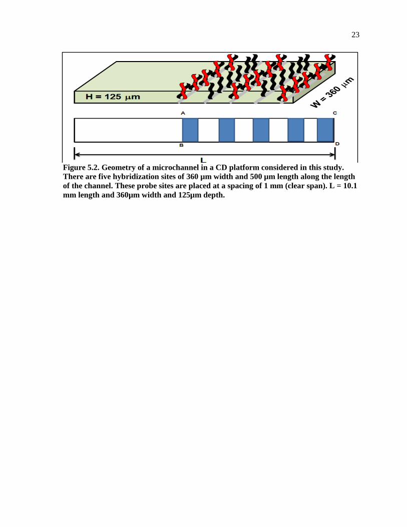
c. 3-D Channel under Various Rotational Speeds: In the third set of examples, we consider the same microchannel described (see Figure 5.2). The 3D microchannel is subjected to a series of angular velocities ω of magnitudes 25, 100, 150, 300, and 350 rad/sec. DNA of 50mM concentration is injected at the channel entrance continuously. There are five hybridization sites of 500µm width and 500µm depth along the length of the channel. These probe sites are placed at a spacing of 1mm. The results of DNA hybridization are shown in Figures 5.3-5.5. In Figure 5.3.a, we show the transient variation of hybridized DNA (dsDNA) at various locations in microchannel under ω = 300 rad/sec. It is clearly shown that for point ‘C’ which is nearer the location of the maximum velocity (as affected by Coriolis force), dsDNA accumulates relatively faster, particularly for the first 0.4 seconds. Once equilibrium is reached, however, accumulations in all the four corner points seem to be approximately the same. Figure 5.3.b shows the effects of the magnitude of angular velocity on dsDNA accumulation on probe sites. As expected, there is a noticeable time lag of about 2 seconds in reaching equilibrium between higher angular velocities (300 rad/sec, for example) and angular velocity of 25 rad/sec.

The effect of channel width on hybridization is summarized in Figure 5.4. The maximum difference is about 10-15% between channels of widths of 500µm and 100µm. In general, the centrifugal force is dominant until the angular velocity reachesa value of 200 rad/sec after which its influence on hybridization is observed. The velocity patterns in most parts of the microchannel - particularly in the middle - do not seem to be affected by Coriolis force. However, at probe sites near to the exit of the microchannel a significant variation in hybridization is observed. For CD platform being rotated in a clockwise direction, the maximum hybridizations are located at the top of the probe sites nearer to the exit. This is expected as the velocities are higher at these regions as shown in the earlier examples.

Whereas, Figure 5.5 shows accumulation of the dsDNA on the zone 1 and zone 5 of the probe sites and from bar chart shows that as the ssDNA goes from zone 1 to zone 5 the accumulation of the dsDNA increases for the different omega ranging from 50 rad/sec to 350 rad/sec.

23

Figure 5.2. Geometry of a microchannel in a CD platform considered in this study. There are five hybridization sites of 360 µm width and 500 µm length along the length of the channel. These probe sites are placed at a spacing of 1 mm (clear span). L = 10.1 mm length and 360µm width and 125µm depth.

24

Figure 5.3. (a) Transient variation of hybridized DNA (dsDNA) at various locations in microchannel under ω = 100 rad/sec., (b) effect of angular velocity on transient variation of hybridized DNA (dsDNA) at various locations in microchannel, and (c) effect of angular velocity on transient variation of hybridized DNA (dsDNA) at various locations in microchannel for ω = 100 rad/sec and ω = 25 rad/sec for non-specific and specific hybridization.

25

a.

b.

26

c.

27

Figure 5.4. (a) Effect of channel width on transient variation of hybridized DNA (dsDNA) at various locations in microchannel, and (b) effect of channel width on transient variation of hybridized DNA (dsDNA) at Point 'C" for ω = 50 rad/sec for non-specific and specific hybridization.

a.

b.

28

Figure 5.5. Accumulation ratios at the different capture probe locations as a function of the angular velocity.

29

CHAPTER 6

NUMERICAL RESULTS AND DISCUSSION FOR

FLUID MIXING

The mixing dynamics in the microchannel is simulated using the commercial finite

element code, Comsol Multiphysics where the laminar Navier-Stoke’s equation is coupled

with convection-diffusion equation for getting the transport of diluted species along the

channel. We consider the two phase flow of NaCl with different concentration of 1 molar and

0 molar in one of the each channel. There are two different types of microchannel are used

one with obstacles and one without obstacles, and the mixing efficiency is measured for each

of the microchannel. The mixing patterns are visualized by the distribution of mixture

fraction at various locations along the microchannel.

The velocity field and the pressure field in the microchannel are governed by the

incompressible Navier-Stoke’s equation.

0. =∇ U (Continuity Equation) (6.1.a)

(Momentum Equation) (6.1.b)

Where, ⍴ is the density of the NaCl is 1030 kg/m3, U is the velocity of the liquid, µ is

the dynamic viscosity of the liquid 6*10-4 and ⍵ is the angular velocity with which the

microchannel is rotated.

Transportation of the molecular species in the microchannel is governed by the Fick’s

second Law, assuming that there is no chemical reaction in the mixture.

(6.2)

Where Ci is the concentration of the species and D is the diffusion coefficient of the liquid.

The schematics of the microchannel with obstacles and without obstacles are shown

in the Figures 6.1 and 6.2 which carries the NaCl solution in one of the each channel having

⍴ of 1030 kg/m3 and η = 6*10-4, the boundary condition are show Table 6.1 and the number

of mesh elements which are used for microchannel without obstacles are 10551 tetrahedral

element

30

Figure 6.1. Microchannel without obstacles.

Figure 6.2. Microchannel with obstacles.

300µm

5 mm

150 µm

300 µm

20µmф

5 mm

150µm

1 mm

31

Table 6.1. Summary of the Boundary Conditions and Constants Used in the Numerical Model for Fluid Mixing in Straight Channel

and microchannel with obstacles have 21439 tetrahedral element (see Figures A.2 and A.3 in

the Appendix). In the simulation the microchannel is rotated at angular velocity of ⍵ = 50

rad/s up to ⍵ = 200 rad/s.

6.1 VELOCITY DISTRIBUTION IN MICROCHANNEL The Velocity in microchannel with and without obstacles is show in Table 6.2 with

maximum velocity for different angular velocity varying from ⍵ = 50 rad/s to ⍵ 200 rad/s.

6.2 CONCENTRATION PLOTS The rate of change in the concentration with respect to time from 0 to 1 sec for

microchannel with and without obstacles for angular velocity of 50 rad/s is show in Table

6.3.

As the angular velocity increase so as the mixing of the two fluid increase the only

difference is that the mixing in the microchannel with obstacles will have faster rate of

change of concentration in compare to the microchannel without any obstacles, and also this

change depends on the speed of rotation which here varies from 50 rad/s to 200 rad/s and is

shown in Figure 6.3 and Figure 6.4 respectively.

Physics Bound. Cond. R (Reaction Term) Constants Fluid Flow (Navier- Stokes Equation)

(Eq. 6.1.a-b)

No slip at all walls.

Inlet

P = 0

Outlet

P = Neutral

Body force = FCentrifugal + FCoriolis

__________________ = 1030 kg/m3

η = 6x10-4 Ns/m2

Convection-Diffusion Equation.

(Eq. 6.2)

@ walls

Insulated (zero flux).

@ outlet

Convective Flux

@ Inlet 1

Concentration (c) = 1.0 molar

@ Inlet 2

Concentration (c) = 0.0 molar

D DNA = 6.8e-11 m2/s [19]

R= 0

U = u m/s

V= v m/s

W= w m/s

32

Table 6.2. Velocity Distributions for Different Omega Angular Velocity (rad/s)

Microchannel with obstacles velocity distribution(v1)

Microchannel with obstacles velocity distribution(v2)

Maximum Velocity(m/s)

⍵ = 200

v1 = 0.426

v2 = 0.405

⍵ = 150

v1 = 0.243

v2 = 0.241

⍵ = 125

v1 = 0.174

v2 = 0.169

⍵ = 100

v1 = 0.114

v2 = 0.112

⍵ = 75

v1 = 0.0652

v2 = 0.0657

⍵ = 50

v1 = 0.0291

v2 = 0.0300

33

Table 6.3. Rate of Change of Concentration with Time

Microchannel withoutObstacles Microchannel with obstacles

t = 0.1 sec t = 0.1 sec

t = 0.2 sec t = 0.2 sec

t = 0.4 sec t = 0.4 sec

t = 0.6 sec t = 0.6 sec

t = 0.8 sec t = 0.8 sec

t = 1 sec t = 1 sec

34

Figure 6.3. Change of concentration at different angular velocity for microchannel without obstacles.

Figure 6.4. Change of concentration at different angular velocity for microchannel with obstacles.

35

6.3 MIXING EFFICIENCY Based on the visualization of the results from simulation here the mixing efficiency is

calculated for both the microchannel at four different location from the entrance of the fluid

which at 1mm, 2mm, 3mm and 4mm distance from the entrance of the channel having length

of 5mm in x-direction using the below equation [16].

(6.3)

Where, Meff is the mixing efficiency of the two fluids, C is the mass concentration of

the two fluids at outlet, C is the concentration of complete mixing and C0 is the initial

distribution of the concentration of the liquid [16] (see Figure 6.5).

Figure 6.5. Mixing efficiency of microchannel without obstacles.

The below plots show the mixing of the two fluid at different location for angular

velocity changing from 50 rad/sec to 200 rad/sec and as the results shows, as the speed

increase so as the mixing of the two fluid due to Coriolis force but in case of microchannel

with obstacles the mixing efficiency is higher than one without the obstacles because in this

even the obstacles also influence the mixing rate of the two fluid [16] (see Figure 6.6, 6.7 and

6.8).

5 mm

36

Figure 6.6. Mixing efficiency of microchannel with obstacles.

Figure 6.7. Mixing efficiency plot of microchannel without obstacles.

37

Figure 6.8. Mixing efficiency plot of microchannel with obstacles.

38

CHAPTER 7

CONCLUSION

In our first study we investigates, through numerical modeling, the influence of

Coriolis forces on the transport and hybridization of DNA in CD microfluidic chips where

centrifugal force is used as the driving force. While the effect of Coriolis force on the fluid

flow in CD microfluidic channels has been studied experimentally and numerically only

recently, its influence on DNA hybridization has not been investigated so far. This study

addresses, therefore, this phenomenon through numerical simulation and demonstrates that

for most practical geometrical configurations and angular velocity ranges reported in the

literature, the Coriolis force introduces significant qualitative and quantitative variations in

DNA hybridization, particularly at locations near the periphery.

In general, the following conclusions are made based on results from this study:

1. This effect is observed to be significantly influenced by channel width and length and angular rotations larger than 100 revolutions per minute. Further, the velocity patterns in the most part of the microchannel, particularly in the middle, do not seem to be affected by Coriolis force.

2. However, at probe sites near to the exit of the microchannel a significant spatial variation in hybridization is observed.

3. For CD platform bring rotated in a clockwise direction, the maximum hybridizations are located at the bottom of the probe sites nearer to the exit.

4. Our results further indicate that the time frame for hybridization is so fast that the effect due to Coriolis force on the location of hybridization is more important than time of hybridization.

5. Our results indicate that for low viscosity fluids, angular velocities as low as 25 rad/sec could introduce Coriolis force that is as high as at least 25% of the main driving centrifugal force. If the channel widths are moderately wide (in the range of 200 microns).

Whereas in our second study for the influence of the Coriolis force on the mixing of

two fluid for microchannel with obstacles and without obstacle shows significant amount of

mixing taking place in microchannel with obstacle in compare to microchannel without

obstacles because over here obstacle also influences the mixing along with the Coriolis force

and centrifugal force. As the speed at which the microchannel is rotated is increased the

mixing taking place between two liquids also increases. By the results obtain one can clearly

39

see the amount of mixing efficiency obtain at the higher speed then at lower speed even

though the obstacles in the microchannel will have different effect on the system.

40

BIBLIOGRAPHY

[1] Ahuja, Satinder. Chromatography and Separation Science. San Diego: Academic Press, 2003.

[2] Benenson, Walter, John. W. Harris, Horst Stocker, and Holger Lutz, eds. Handbook of Physics. New York: Springer, 2002.

[3] Brenner, Thilo, Markus Grumann, Christian Beer, Roland Zengerle, and Jens Ducrée. “Microscopic Characterization of Flow Patterns in Rotating Microchannels.” Paper presented at the Proceedings of MICRO.Tec, Munich, Germany, October 2003.

[4] Brenner, Thilo. “Polymer Fabrication and Microfluidic Unit Operations for Medical Diagnostics on a Rotating Disk.” PhD diss., University of Freiburg, 2005. http:// www.freidok.uni-freiburg.de/volltexte/2306/pdf/Diss_Brenner.pdf

[5] Brenner, Thilo, Roland Zengerle, and Jens Ducrée. “A Flow-Switch Based on Coriolis Force.” Paper presented at the 7th International Conference on Miniaturized Chemical and Biochemical Analysis Systems, Squaw Valley, CA, October 2003.

[6] Chakraborty, Suman, ed. Microfluidics and Microfabrications. New York: Springer, 2010.

[7] Cho, Yoon-Kyoung, Jeong-Gun Lee, Jong-Myeon Park, Beom-Seok Lee, Youngsun Lee, and Christopher Ko. “One-Step Pathogen Specific DNA Extraction from Whole Blood on a Centrifugal Microfluidic Device.” Lab on a Chip 7, no. 5 (2007): 565-73.

[8] Das, Siddhartha, and Suman Chakraborty. “Transverse Electrodes for Improved DNA Hybridization in Microchannels.” AIChE Journal 53, no. 5 (2007): 1086-99.

[9] Das, Siddhartha, Tamal Das, and Suman Chakraborty. “Analytical Solutions for the Rate of DNA Hybridization in a Microchannel in the Presence of Pressure-Driven and Electroosmotic Flows.” Sensors and Actuators B: Chemical 114, no. 2 (April 2006): 957-63.

[10] Ducrée, Jens, Thilo Brenner, Stefan Haeberle, Thomas Glatzel, and Roland Zengerle. “Multilamination of Flows in Planar Networks of Rotating Microchannels.” Journal of Microfluidics and Nanofluidics 2, no. 1 (2006): 78-84.

[11] Ducrée, Jens, Thilo Brenner, Stefan Haeberle, Thomas Glatzel, and Roland Zengerle. “Patterning of Flow and Mixing in Rotating Radial Microchannels.” Microfluidics & Nanofluidics 2, no. 2 (2005): 97-105.

[12] Ducrée, Jens, Thilo Brener, Thomas Glatzel, and Roland Zengerle. “Coriolis-Induced Switching and Mixing of Laminar Flows in Rotating Microchannels.” Paper presented at the Proceedings of Micro Technology, Munich, Germany, October 2003.

[13] Duffy, David C., Heather L. Gills, Joe Lin, Norman F. Sheppard, and Gregory J. Kellogg. “Microfabicated Centrifugal Microfluidic Systems: Characterization and Multiple Enzymatic Assays.” Analytical Chemistry 71, no. 20 (1999): 4669–78.

41

[14] Erickson, David, Dongqing Li, and Ulrich J. Krull. “Modelling of DNA Hybridization Kinetics for Spatially Resolved Biochips.” Analytical Biochemistry 317, no. 2 (2003): 186-200.

[15] Haeberle, Stefan, Thilo Brenner, Roland Zengerle, and Jens Ducrée. “Centrifugal Extraction of Plasma from Whole Blood on a Rotating Disk.” Lab on a Chip 6, no. 1 (2006): 776-81.

[16] Hsieh, Shou-Shing, and Yi-Cheng Huang. “Passive Mixing in Microchannel with Geometric Variation Through µPIV and µLIF Measurement.” Journal of Mechanical and Microengineeing 18, no. 6 (2008): 65017.

[17] Jia, Guangyao, Kuo-Sheng Ma, Jitae Kim, Jim V. Zoval, Regis Peytavi, Michel G. Bergeron, and Marc J. Madou. “Dynamic Automated DNA Hybridization on a CD (Compact Disc) Fluidic Platform.” Sensors and Actuators B: Chemical 114, no. 1 (2006): 173-81.

[18] Kassegne, Sam, Bhuvnesh Arya, and Neeraj Yadav. “Numerical Modeling of the Effect of Histidine Protonation on DNA Hybridization and pH Distribution in Electronically Active Microarrays.” Sensors and Actuators B 143, no. 2 (2010): 470-81.

[19] Kassegne, Samuel K., Howard Reese, Dalibor Hodko, Joon M. Yang, Kamal Sarkar, Dan Smolko, Paul Swanson, Daniel E. Raymond, Michael J. Heller, and Marc J. Madou. “Numerical Modeling of Transport and Accumulation of DNA on Electronically Active Biochips.” Journal of Sensors and Actuators B: Chemical 94, no. 1 (2003) 81–98.

[20] Kellogg, Gregory J., Todd E. Arnold, Bruce L. Carvalho, David C. Duffy, and Norman F. Sheppard. “Centrifugal Microfluidics: Applications.” In Micro Total Analysis Systems 2000, edited by Albert van den Berg, Wouter Olthuis, and Piet Bergveld, 239-42. Amsterdam: Kluwer Academic, 2000.

[21] Kim, Jitae, Horacio Kido, Roger H. Rangel, and Marc J. Madou. “Passive Flow Switching Valves on a Centrifugal Microfluidic Platform.” Sensors & Actuators: B. Chemical 128, no. 2 (January 2008): 613-21.

[22] Kim, Joshua Hyong-Seok, Alia Marafie, Xi-Yu Jia, Jim V. Zoval, and Marc J. Madou. “Characterization of DNA Hybridization Kinetics in a Microfluidic Flow Channel.” Sensors and Actuators B: Chemical 113, no. 1 (January 2006): 281-89.

[23] Kim, Nahui, Catherine M. Dempsey, Jim V. Zoval, Ji-Ying Sze, and Marc J. Madou. “Automated Microfluidic Compact Disc (CD) Cultivation System of Caenorhabditis Elegans.” Sensors and Actuators B: Chemical 122, no. 2 (March 2007): 511-18.

[24] Madou, Marc, and Gregory J. Kellogg. “LabCD: A Centrifuge-Based Microfluidic Platform for Diagnostics.” In Systems and Technologies for Clinical Diagnostics and Drug Discovery, edited by Gerald E. Cohn, 80-93. San Jose: SPIE, 1998.

[25] Madou, Marc, Jim Zoval, Guangyao Jia, Horacio Kido, Jitae Kim, and Nahui Kim. “Lab on a Disc, Annual Review of Biomedical Engineering.” Annual Review of Biomedical Engineering 8, no. 1 (August 2006): 601-28.

42

[26] Madou, Marc, L. James Lee, Sylvia Daunert, Siyi Lai, and Chih-Hsin Shih. “Design and Fabrication of CD-Like Microfluidic Platforms for Diagnostics: Microfluidic Functions.” Biomedical Microdevices 3, no. 3 (2001): 245-54.

[27] Madou, Marc, Y. Lu, S. Lai, J. Lee, and S. Daunert. “A Centrifugal Microfluidic Platform: A Comparison.” In Micro Total Analysis Systems 2000, edited by Albert van den Berg, Wouter Olthuis, and Piet Bergveld, 565-70. Amsterdam: Kluwer Academic, 2000.

[28] Nguyen, Nam-Trung, and Steven. T. Wereley. Fundamentals and Application of Microfluidics. Boston: Artech House, 2002.

[29] Pappaert, Kris, and Gert Desmet. “A Dimensionless Number Analysis of the Hybridization Process in Diffusion- and Convection-Driven DNA Microarray Systems.” Journal of Biotechnology 123, no. 4 (2006): 381-96.

[30] Riegger, Lutz, Markus Grumann, J. Steigert, Sascha Lutz, C. P. Steinert, C. Meuller, J. Viertel, Oswald Prucker, J. Ruhe, Roland Zengerle, and Jens Ducrée. “Single-Step Centrifugal Hematocrit Determination on a 10-$ Processing Device.” Biomedical Microdevices 9, no. 6 (2007): 795-99.

[31] Riegger, Lutz, Markus Grumann, Thomas Nann, Jurgen Riegler, Oliver Ehlert, K. Mittenbühler, G. Urban, Lars Pastewka, Thilo Brenner, Roland Zengerle, and Jens Ducrée. “Readout Concept for Multiplexed Bead-Based Fluorescence Immunoassays on Centrifugal Microfluidic Platforms.” Sensors and Actuators A: Physical 126, no. 2 (2006): 455-62.

[32] Rothert, Anna, Lori Millner, Libby G. Puckett, Sapna K. Deo, Marc J. Madou, and Sylvia Daunert, “Whole Cell Reporter Gene-Based Biosensing Systems on a Compact Disc Microfluidics Platform.” Analytical Biochemistry 342, no. 1 (2005): 11-19.

[33] Schilling, Eric. “Basic Microfluidic Concepts.” September 7, 2001. http://faculty. washington.edu/yagerp/microfluidicstutorial/basicconcepts/basicconcepts.htm.

[34] Zeng, Jun, Deb Banerjee, Manish Deshpande, John R. Gilbert, David C. Duffy, and Gregory J. Kellogg. “Design Analysis of Capillary Burst Valves in Centrifugal Microfluidics.” In Micro Total Analysis Systems 2000, edited by Albert van den Berg, Wouter Olthuis, and Piet Bergveld, 579–82. Amsterdam: Kluwer Academic, 2000.

[35] Zhang, Jinlong, Qiuquan Guo, Mei Liu, and Jun Yang. “A Lab-On-CD Prototype for High-Speed Blood Separation.” Journal of Micromechanics and Microengineering 18, no. 12 (2008): 125025.

43

APPENDIX

MESHED GEMETRY FOR STRAIGHT

CHANNELS

44

A.1 CORIOLIS INDUCED HYBRIDIZATION

Figure A.1. Straight channel ~10mm length.

Grid of DNA Hybridization in straight channel

View- Isometric view of straight channel of 125µm height with grids

Grid Size- 62158 tetrahedral elements

Solver- Direct (UMFPACK)

45

A.2 CORIOLIS INDUCED MIXING IN STRAIGHT CHANNEL WITHOUT OBSTACLES

Figure A.2. Straight channel ~5mm length.

Grid view of straight channel without obstacles

View- Isometric view of straight channel without obstacle of 150µm height with grids

Grid Size- 10551 tetrahedral elements

Solver- Direct (UMFPACK)

46

A.3 CORIOLIS INDUCED MIXING IN STRAIGHT CHANNEL WITH OBSTACLES

Figure A.3. Straight channel with obstacles.

Grid view of straight channel with obstacles

View- Isometric view of straight channel with obstacle of 150µm height with grids

Grid Size- 21439 tetrahedral elements

Solver- Direct (PARDISO)