UNT Ionospheric radars development - Earth-prints
155
UNT Ionospheric radars development The following slides were presented during the lectures of the course “Desarrollo de radares ionosféricos” held within the post graduate course on “Geofísica espacial” organised by the Universidad Nacional de Tucumán - Facultad de Ciencias Exactas y Tecnología - Departamento de Posgrado in Tucumán on 4 – 7 October 2010. Enrico Zuccheretti, Umberto Sciacca [email protected] - [email protected] Istituto Nazionale di Geofisica e Vulcanologia - Rome, Italy
Transcript of UNT Ionospheric radars development - Earth-prints
UNT
Ionospheric radars development
The following slides were presented during the lectures of the course
“Desarrollo de radares ionosféricos” held within the post graduate
course on “Geofísica espacial” organised by the Universidad
Nacional de Tucumán - Facultad de Ciencias Exactas y Tecnología -
Departamento de Posgrado in Tucumán on 4 – 7 October 2010.
Enrico Zuccheretti, Umberto Sciacca
[email protected] - [email protected]
Istituto Nazionale di Geofisica e Vulcanologia - Rome, Italy
UNT
Module 1
Basics of radar theory
and design elements
UNT
•The ionosphere is no exception: the most common way to study its behaviour is to emit radio wave pulses into the ionosphere and to study the backscattered echo.
•The echo signal contains information about the layers in which it may be refracted, reflected or absorbed.
•Also signals coming from satellites (NNSS, GPS) or from terrestrial emitting station (VLF emitters) can be used. They do not exploit the radar technique but their properties are affected by the medium they pass through.
•Amongst the big variety of techniques used to study the geophysical environment, methods using electromagnetic waves occupy a very prominent position.
•These techniques exploit radio waves modifications when they interact with the medium they pass through.
Introduction
UNT
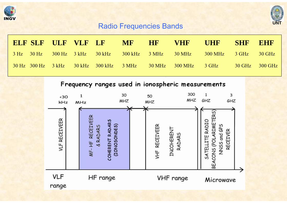
ELF3 Hz
30 Hz
SLF30 Hz
300 Hz
ULF300 Hz
3 kHz
VLF3 kHz
30 kHz
LF30 kHz
300 kHz
MF300 kHz
3 MHz
HF3 MHz
30 MHz
VHF30 MHz
300 MHz
UHF300 MHz
3 GHz
SHF3 GHz
30 GHz
EHF30 GHz
300 GHz
Radio Frequencies Bands
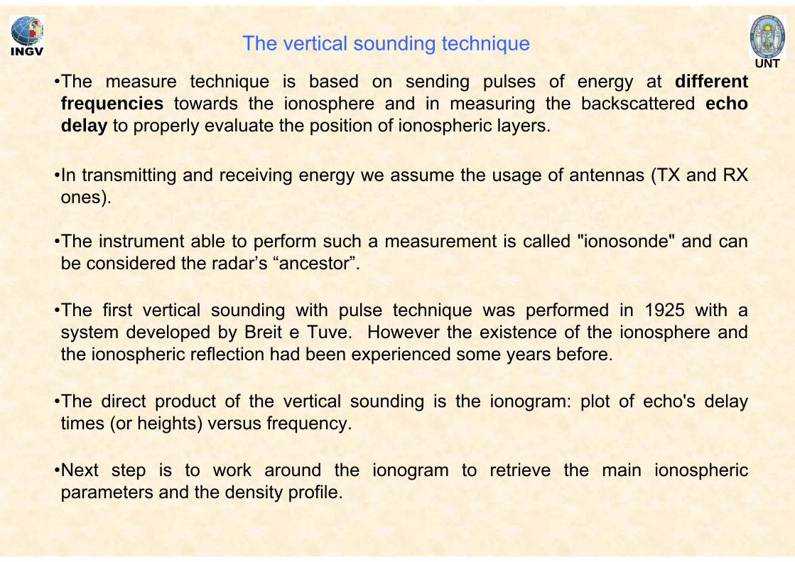
UNT•The measure technique is based on sending pulses of energy at different frequencies towards the ionosphere and in measuring the backscattered echo delay to properly evaluate the position of ionospheric layers.
The vertical sounding technique
•In transmitting and receiving energy we assume the usage of antennas (TX and RX ones).
•The instrument able to perform such a measurement is called "ionosonde" and can be considered the radar’s “ancestor”.
•The first vertical sounding with pulse technique was performed in 1925 with a system developed by Breit e Tuve. However the existence of the ionosphere and the ionospheric reflection had been experienced some years before.
•The direct product of the vertical sounding is the ionogram: plot of echo's delay times (or heights) versus frequency.
•Next step is to work around the ionogram to retrieve the main ionospheric parameters and the density profile.
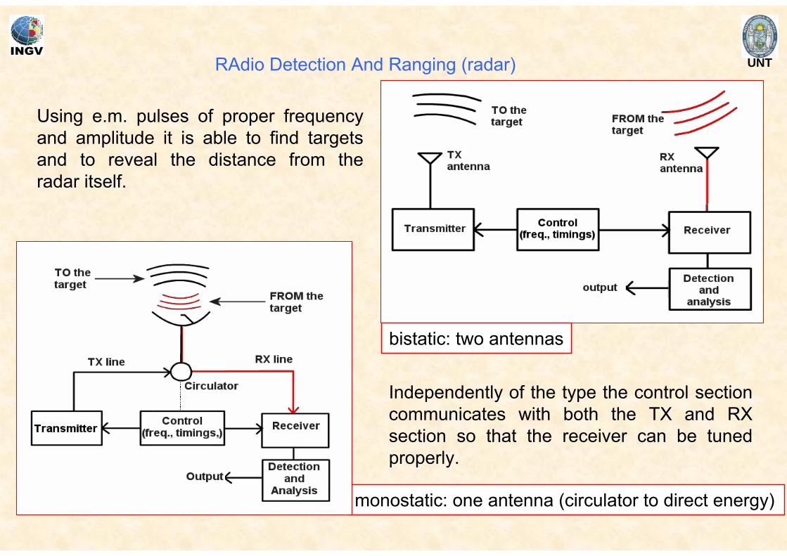
UNTRAdio Detection And Ranging (radar)
Independently of the type the control section communicates with both the TX and RX section so that the receiver can be tuned properly.
Using e.m. pulses of proper frequency and amplitude it is able to find targets and to reveal the distance from the radar itself.
monostatic: one antenna (circulator to direct energy)
bistatic: two antennas
UNT
43
2
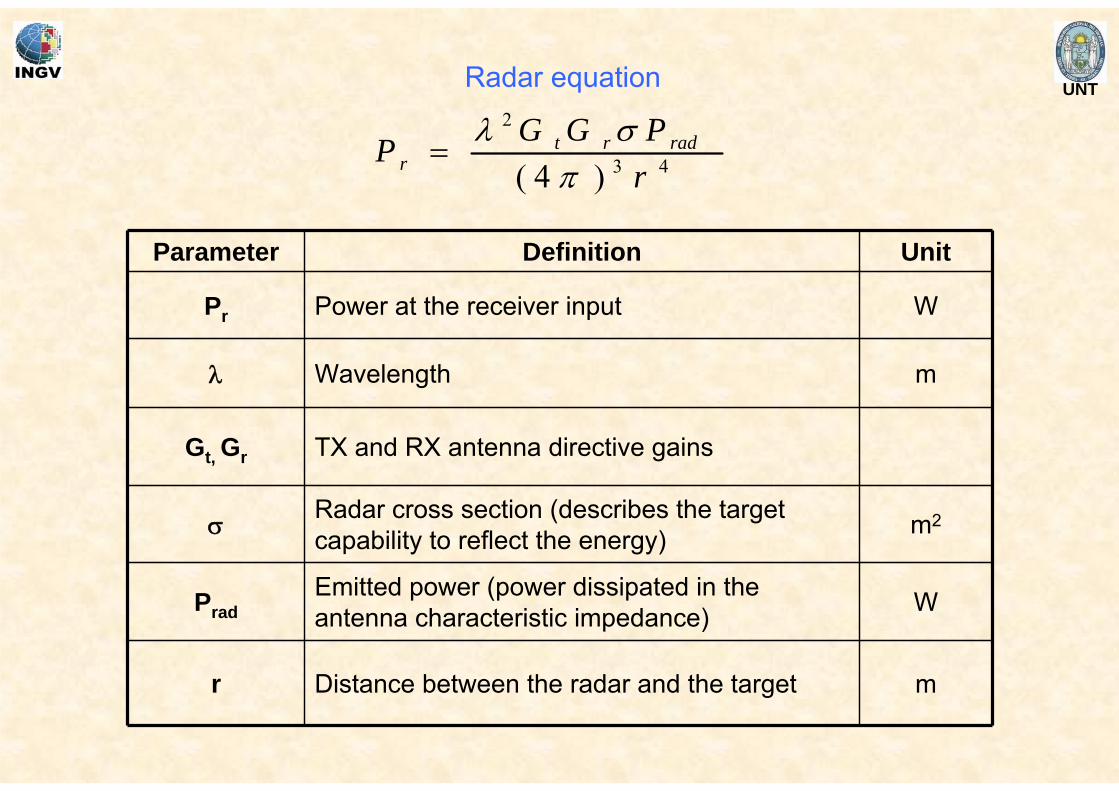
)4( rPGGP radrt
r πσλ
=
Parameter Definition Unit
Pr Power at the receiver input W
λ Wavelength m
Gt, Gr TX and RX antenna directive gains
σ Radar cross section (describes the target capability to reflect the energy) m2
PradEmitted power (power dissipated in the antenna characteristic impedance) W
r Distance between the radar and the target m
Radar equation
UNT
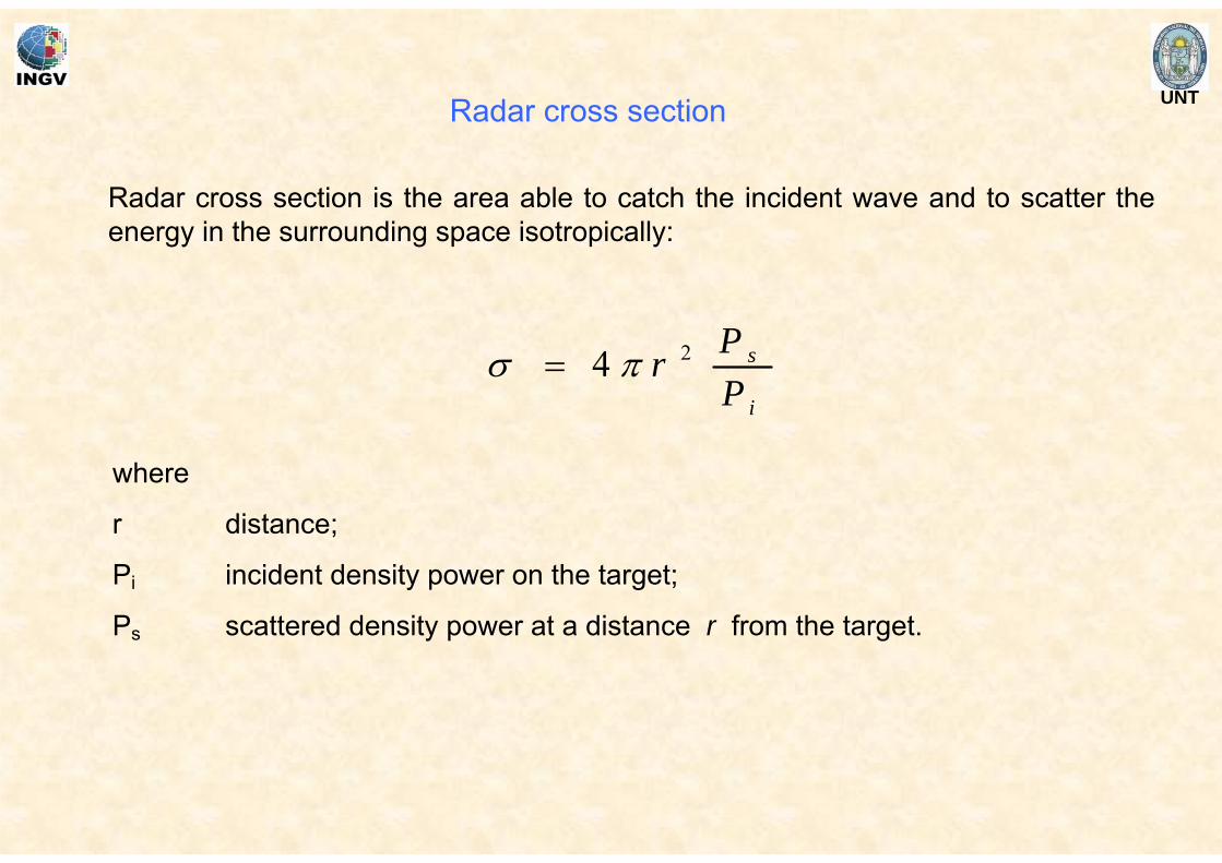
Radar cross section is the area able to catch the incident wave and to scatter the energy in the surrounding space isotropically:
i
s
PPr 24 πσ =
where
r distance;
Pi incident density power on the target;
Ps scattered density power at a distance r from the target.
Radar cross section
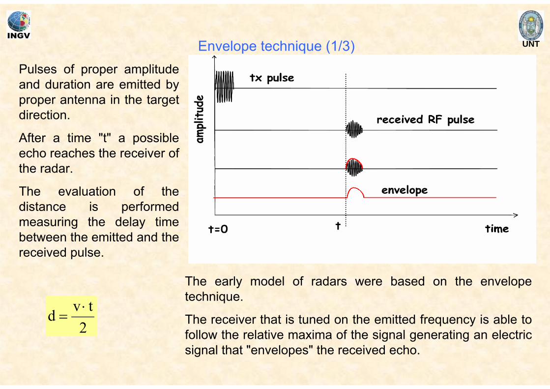
UNTEnvelope technique (1/3)
The early model of radars were based on the envelope technique.
The receiver that is tuned on the emitted frequency is able to follow the relative maxima of the signal generating an electric signal that "envelopes" the received echo.
Pulses of proper amplitude and duration are emitted by proper antenna in the target direction.
After a time "t" a possible echo reaches the receiver of the radar.
The evaluation of the distance is performed measuring the delay time between the emitted and the received pulse.
2tvd ⋅
=
UNT
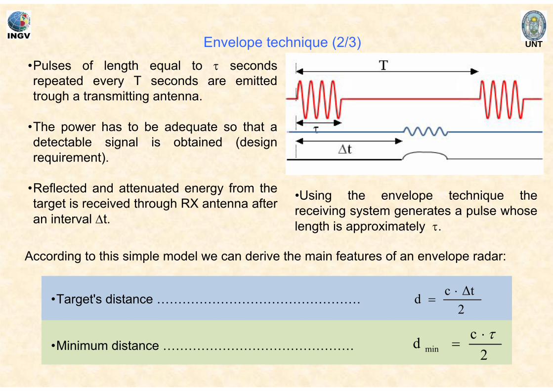
•Pulses of length equal to τ seconds repeated every T seconds are emitted trough a transmitting antenna.
•The power has to be adequate so that a detectable signal is obtained (design requirement).
•Reflected and attenuated energy from the target is received through RX antenna after an interval Δt.
•Using the envelope technique the receiving system generates a pulse whose length is approximately τ.
2Δtcd ⋅
=•Target's distance …………………………………………
2cd min
τ⋅=•Minimum distance ………………………………………
According to this simple model we can derive the main features of an envelope radar:
Envelope technique (2/3)
UNT
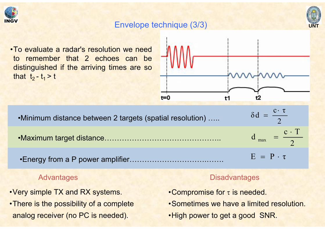
Advantages Disadvantages
•Compromise for τ is needed.•Sometimes we have a limited resolution.•High power to get a good SNR.
•Very simple TX and RX systems.•There is the possibility of a complete analog receiver (no PC is needed).
•To evaluate a radar's resolution we need to remember that 2 echoes can be distinguished if the arriving times are so that t2 - t1 > t
2τcdδ ⋅
=•Minimum distance between 2 targets (spatial resolution) …..
τPE ⋅=•Energy from a P power amplifier………………………….…….
2Tcd max
⋅=•Maximum target distance………………………………………..
Envelope technique (3/3)
UNT
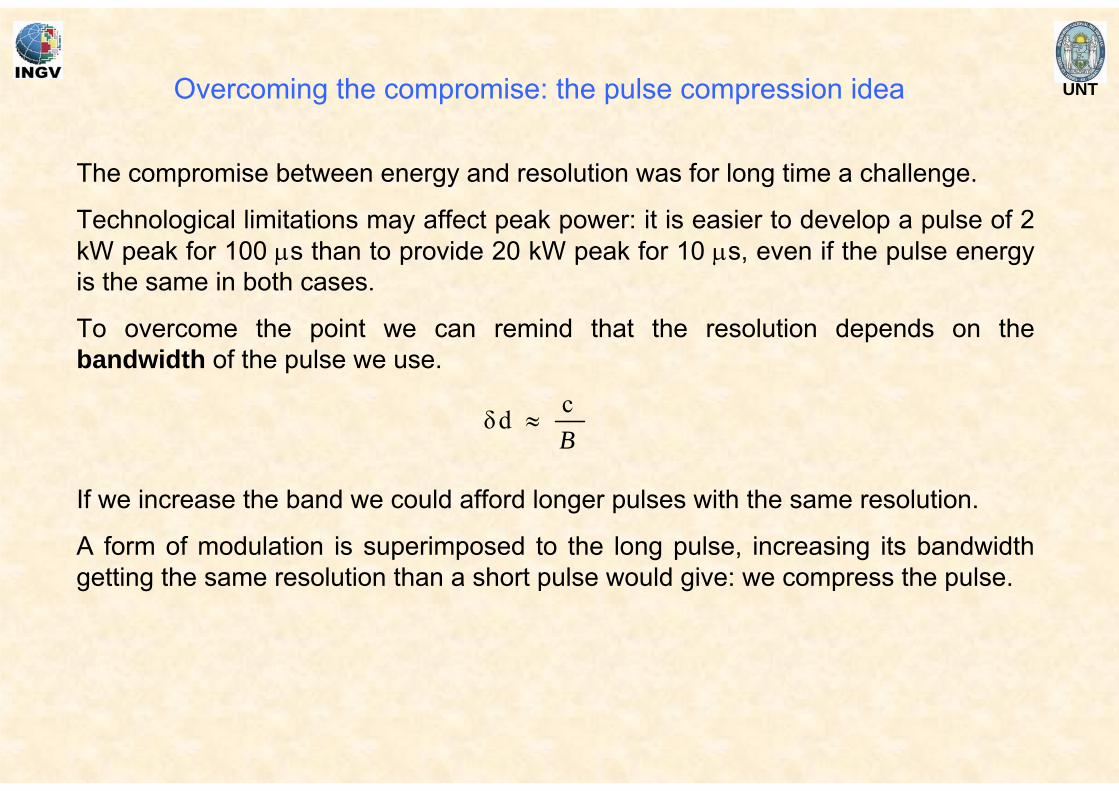
The compromise between energy and resolution was for long time a challenge.
Technological limitations may affect peak power: it is easier to develop a pulse of 2 kW peak for 100 μs than to provide 20 kW peak for 10 μs, even if the pulse energy is the same in both cases.
To overcome the point we can remind that the resolution depends on the bandwidth of the pulse we use.
If we increase the band we could afford longer pulses with the same resolution.
A form of modulation is superimposed to the long pulse, increasing its bandwidth getting the same resolution than a short pulse would give: we compress the pulse.
Bcdδ ≈
Overcoming the compromise: the pulse compression idea
UNT
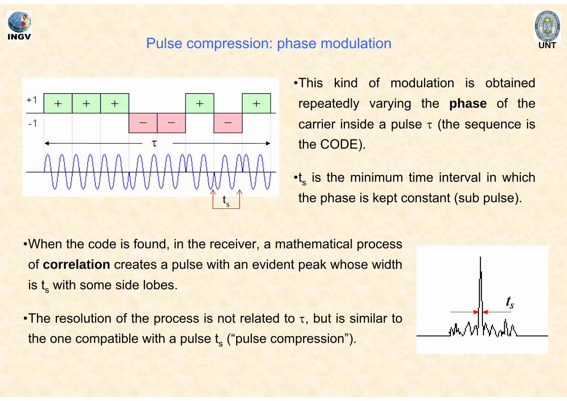
•This kind of modulation is obtained repeatedly varying the phase of the carrier inside a pulse τ (the sequence is the CODE).
•ts is the minimum time interval in which the phase is kept constant (sub pulse).
•When the code is found, in the receiver, a mathematical process of correlation creates a pulse with an evident peak whose width is ts with some side lobes.
•The resolution of the process is not related to τ, but is similar to the one compatible with a pulse ts (“pulse compression”).
ts
τ
Pulse compression: phase modulation
UNT
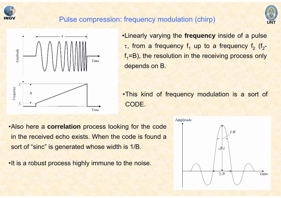
•Linearly varying the frequency inside of a pulse τ, from a frequency f1 up to a frequency f2 (f2-f1=B), the resolution in the receiving process only depends on B.
•Also here a correlation process looking for the code in the received echo exists. When the code is found a sort of “sinc” is generated whose width is 1/B.
•It is a robust process highly immune to the noise.
Pulse compression: frequency modulation (chirp)
•This kind of frequency modulation is a sort of CODE.
UNT
τ
Δt
TTτ
Δt
ts
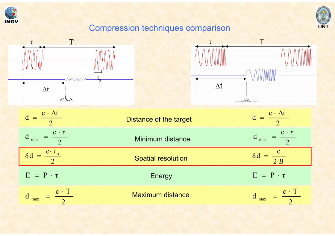
Spatial resolution
Distance of the target
Minimum distance
Maximum distance
Energy
2cd min
τ⋅=
τPE ⋅=
2Tcd max
⋅=
B2cdδ =
2Δtcd ⋅
=
2cd min
τ⋅=
τPE ⋅=
2Tcd max
⋅=
2cdδ st⋅
=
2Δtcd ⋅
=
Compression techniques comparison
UNT
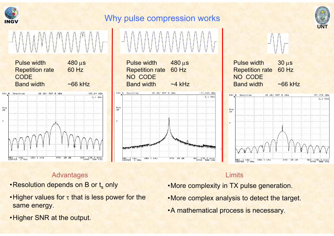
Pulse width 480 μs Repetition rate 60 HzCODEBand width ~66 kHz
Pulse width 480 μs Repetition rate 60 HzNO CODEBand width ~4 kHz
Pulse width 30 μs Repetition rate 60 HzNO CODEBand width ~66 kHz
Why pulse compression works
Advantages Limits•Resolution depends on B or ts only
•Higher values for τ that is less power for the same energy.
•Higher SNR at the output.
•More complexity in TX pulse generation.
•More complex analysis to detect the target.
•A mathematical process is necessary.
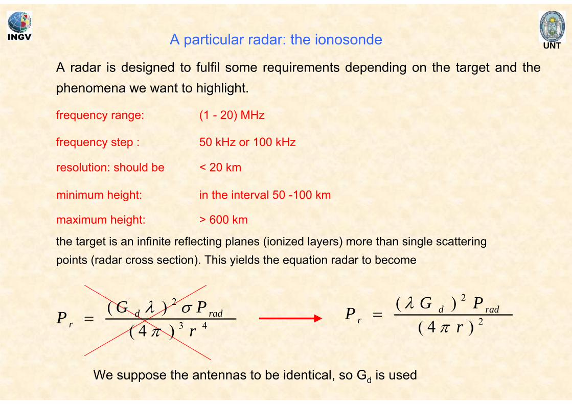
UNTA particular radar: the ionosonde
A radar is designed to fulfil some requirements depending on the target and the phenomena we want to highlight.
frequency range: (1 - 20) MHz
resolution: should be < 20 km
minimum height: in the interval 50 -100 km
maximum height: > 600 km
the target is an infinite reflecting planes (ionized layers) more than single scatteringpoints (radar cross section). This yields the equation radar to become
We suppose the antennas to be identical, so Gd is used
2
2
)4()(r
PGP raddr π
λ=
43
2
)4()(
rPGP radd
r πσλ
=
frequency step : 50 kHz or 100 kHz
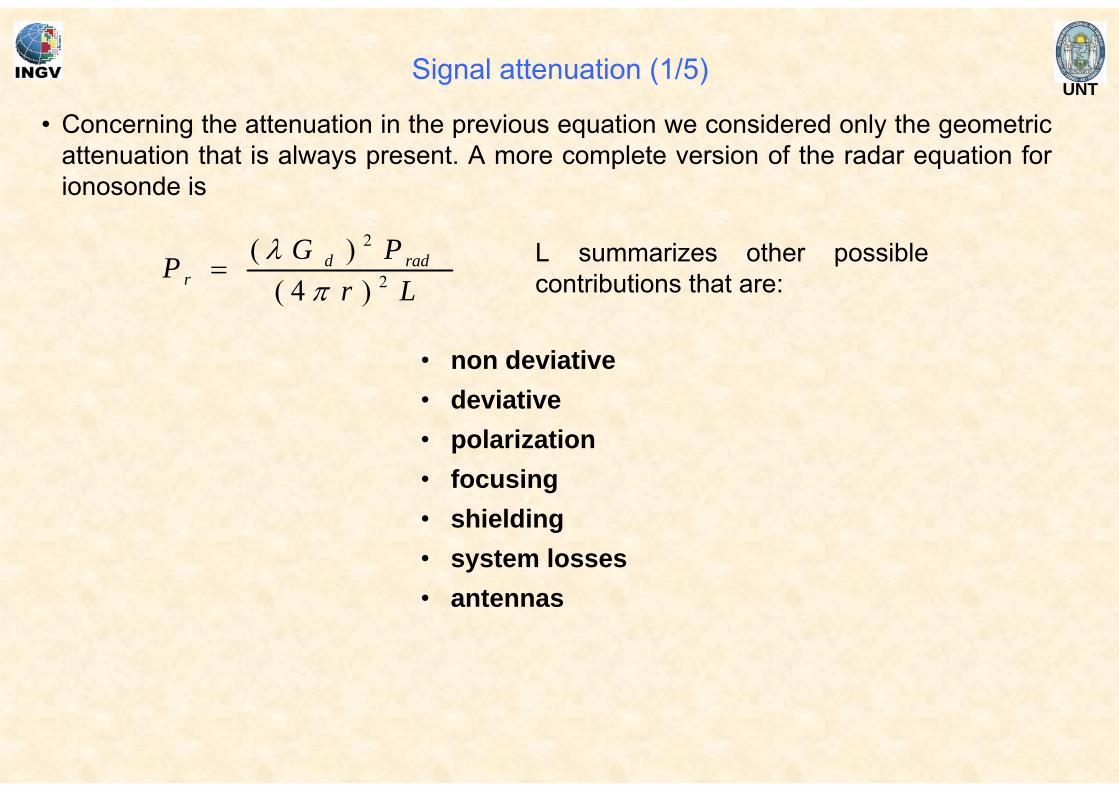
UNTSignal attenuation (1/5)
• Concerning the attenuation in the previous equation we considered only the geometric attenuation that is always present. A more complete version of the radar equation for ionosonde is
LrPGP radd
r 2
2
)4()(
πλ
= L summarizes other possible contributions that are:
• non deviative• deviative• polarization• focusing• shielding• system losses• antennas
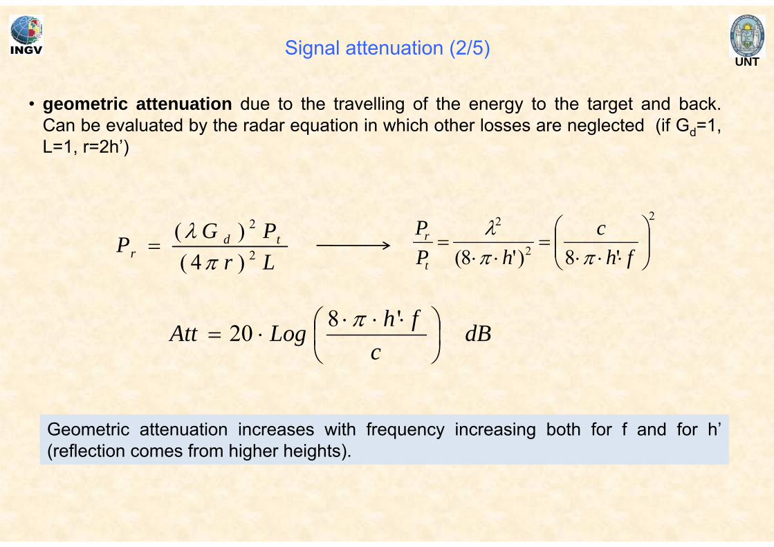
UNT
• geometric attenuation due to the travelling of the energy to the target and back. Can be evaluated by the radar equation in which other losses are neglected (if Gd=1, L=1, r=2h’)
LrPGP td
r 2
2
)4()(
πλ
=
dBc
fhLogAtt ⎟⎠⎞
⎜⎝⎛ ⋅⋅⋅
⋅='820 π
2
2
2
'8)'8( ⎟⎟⎠
⎞⎜⎜⎝
⎛⋅⋅⋅
=⋅⋅
=fh
chP
P
t
r
ππλ
Geometric attenuation increases with frequency increasing both for f and for h’(reflection comes from higher heights).
Signal attenuation (2/5)
UNT
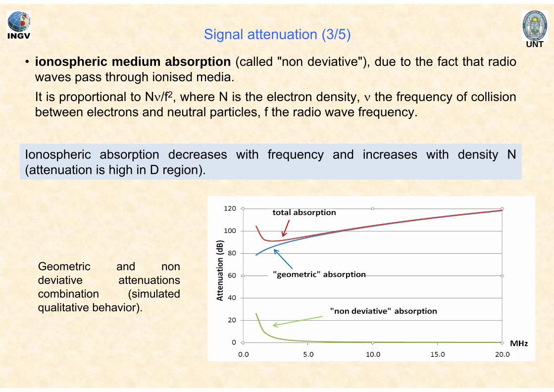
Geometric and non deviative attenuations combination (simulated qualitative behavior).
• ionospheric medium absorption (called "non deviative"), due to the fact that radio waves pass through ionised media.It is proportional to Nν/f2, where N is the electron density, ν the frequency of collision between electrons and neutral particles, f the radio wave frequency.
Ionospheric absorption decreases with frequency and increases with density N (attenuation is high in D region).
Signal attenuation (3/5)
UNT
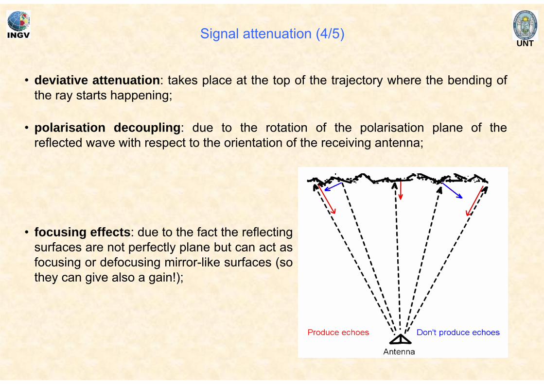
• focusing effects: due to the fact the reflecting surfaces are not perfectly plane but can act as focusing or defocusing mirror-like surfaces (so they can give also a gain!);
• polarisation decoupling: due to the rotation of the polarisation plane of the reflected wave with respect to the orientation of the receiving antenna;
• deviative attenuation: takes place at the top of the trajectory where the bending of the ray starts happening;
Signal attenuation (4/5)
UNT
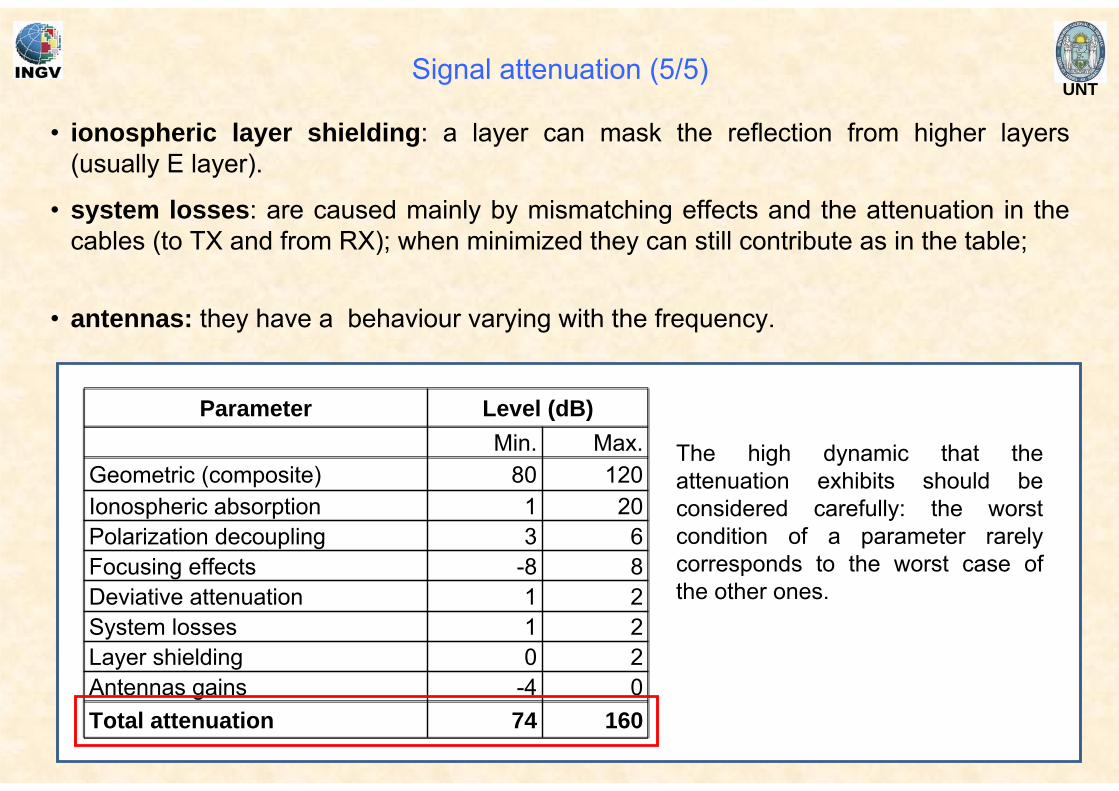
Parameter Level (dB)Min. Max.
Geometric (composite) 80 120Ionospheric absorption 1 20Polarization decoupling 3 6Focusing effects -8 8Deviative attenuation 1 2System losses 1 2Layer shielding 0 2Antennas gains -4 0Total attenuation 74 160
• antennas: they have a behaviour varying with the frequency.
• system losses: are caused mainly by mismatching effects and the attenuation in the cables (to TX and from RX); when minimized they can still contribute as in the table;
The high dynamic that the attenuation exhibits should be considered carefully: the worst condition of a parameter rarely corresponds to the worst case of the other ones.
• ionospheric layer shielding: a layer can mask the reflection from higher layers (usually E layer).
Signal attenuation (5/5)
UNT
• Noise is any cause of degradation of the useful signal due to other signals, coming from various sources.
Noise sources (1/4)
• We can distinguish between internal sources (generated inside the system) and external source (natural and interferences).
• Usually the term is used only referring to signals with a stochastic nature, i.e. not deterministic; we shall use the term in the more general sense, including also the deterministic signals coming from transmitters, other than the ionosonde.
UNT
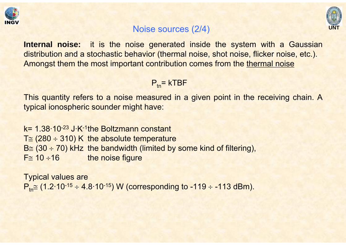
Internal noise: it is the noise generated inside the system with a Gaussian distribution and a stochastic behavior (thermal noise, shot noise, flicker noise, etc.).Amongst them the most important contribution comes from the thermal noise
Ptn= kTBF
This quantity refers to a noise measured in a given point in the receiving chain. A typical ionospheric sounder might have:
k= 1.38·10-23 J·K-1the Boltzmann constantT≅ (280 ÷ 310) K the absolute temperatureB≅ (30 ÷ 70) kHz the bandwidth (limited by some kind of filtering),F≅ 10 ÷16 the noise figure
Typical values are Ptn≅ (1.2·10-15 ÷ 4.8·10-15) W (corresponding to -119 ÷ -113 dBm).
Noise sources (2/4)
UNT
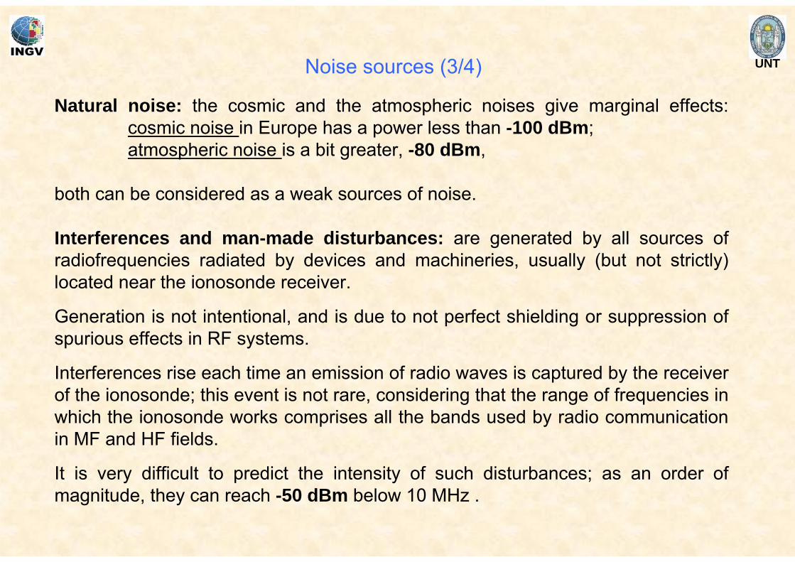
Interferences and man-made disturbances: are generated by all sources of radiofrequencies radiated by devices and machineries, usually (but not strictly) located near the ionosonde receiver.
Generation is not intentional, and is due to not perfect shielding or suppression of spurious effects in RF systems.
Interferences rise each time an emission of radio waves is captured by the receiver of the ionosonde; this event is not rare, considering that the range of frequencies in which the ionosonde works comprises all the bands used by radio communication in MF and HF fields.
It is very difficult to predict the intensity of such disturbances; as an order of magnitude, they can reach -50 dBm below 10 MHz .
Natural noise: the cosmic and the atmospheric noises give marginal effects: cosmic noise in Europe has a power less than -100 dBm;atmospheric noise is a bit greater, -80 dBm,
both can be considered as a weak sources of noise.
Noise sources (3/4)
UNT
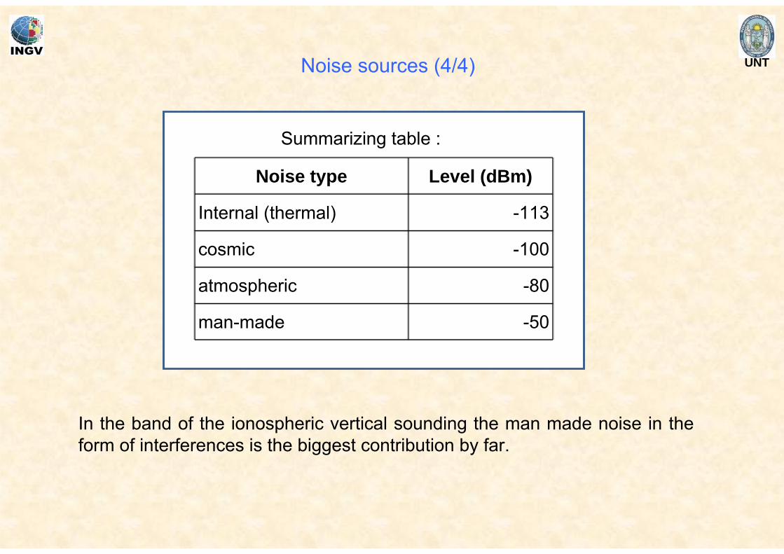
Summarizing table :
Noise type Level (dBm)
Internal (thermal) -113
cosmic -100
atmospheric -80
man-made -50
In the band of the ionospheric vertical sounding the man made noise in the form of interferences is the biggest contribution by far.
Noise sources (4/4)
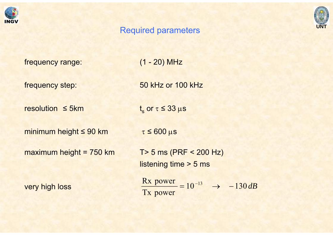
UNTRequired parameters
frequency step: 50 kHz or 100 kHz
resolution ≤ 5km ts or τ ≤ 33 μs
minimum height ≤ 90 km τ ≤ 600 μs
maximum height = 750 km T> 5 ms (PRF < 200 Hz)listening time > 5 ms
dB13010powerTx powerRx 13 −→= −very high loss
frequency range: (1 - 20) MHz
UNT
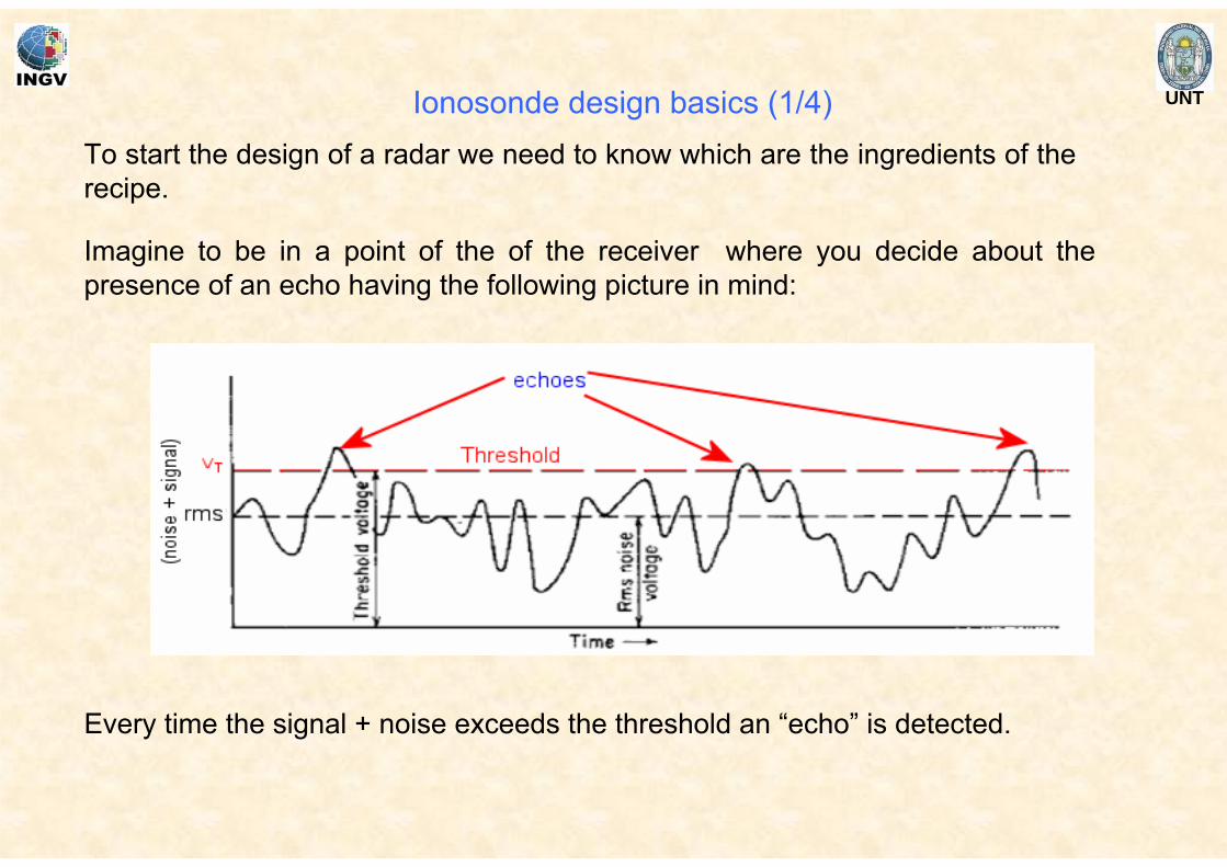
Every time the signal + noise exceeds the threshold an “echo” is detected.
To start the design of a radar we need to know which are the ingredients of the recipe.
Imagine to be in a point of the of the receiver where you decide about the presence of an echo having the following picture in mind:
Ionosonde design basics (1/4)

UNT
The idea of probability comes from the fact that the radar signal process detection is basically statistical in nature due to the nature of the noise voltage that is always present in the receiver circuit.
We can definePd probability of detection: probability of that an echo is detected, when
presentPfa probability of false alarm: probability that a noise fluctuation is mistaken for a
signal.
Pd and Pfa are both functions of VT, signal and noise
targets in the realitytargets’ detection present absentpresent ok (Pd) no (Pfa)absent no (1-Pd) ok (1-Pfa)
We want to have high Pd and low Pfa
This two parameters are enough to describe all possible cases.
Ionosonde design basics (2/4)
UNT
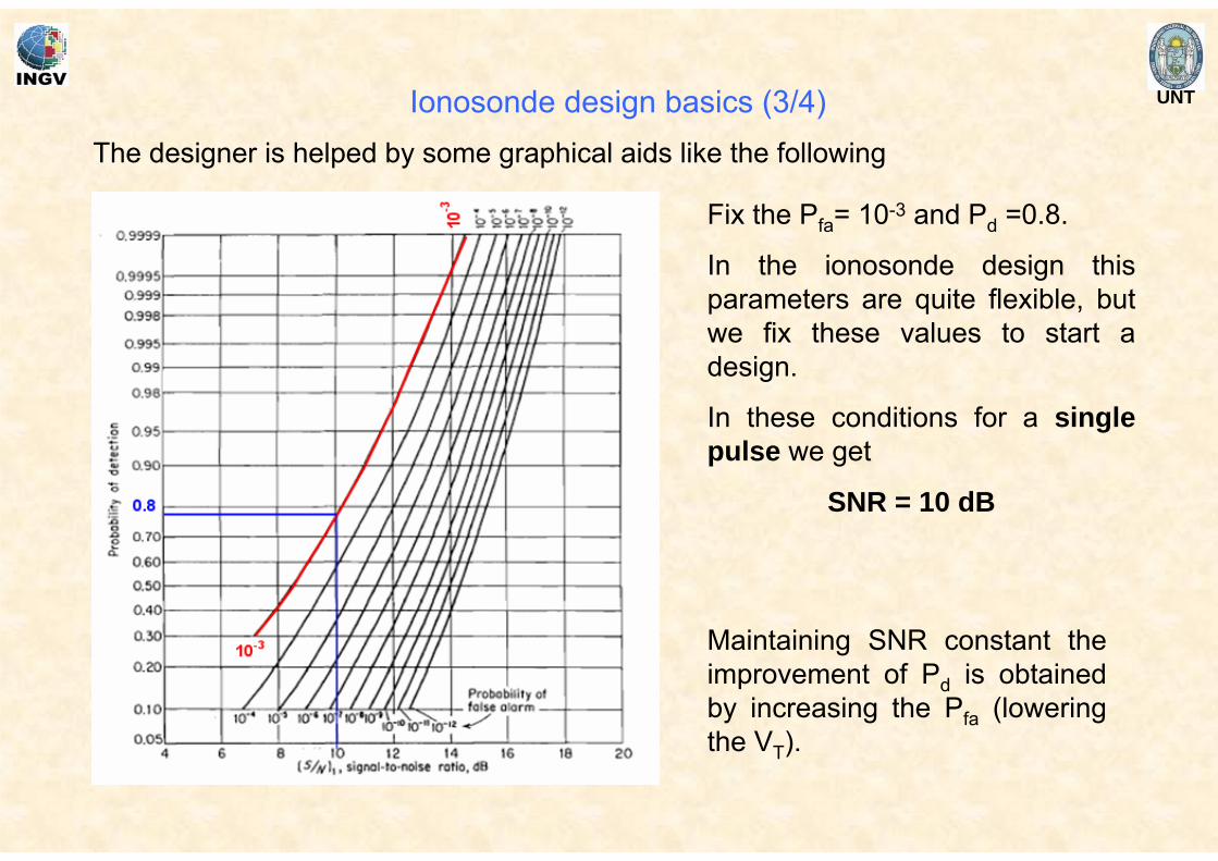
The designer is helped by some graphical aids like the following
Fix the Pfa= 10-3 and Pd =0.8.
In the ionosonde design this parameters are quite flexible, but we fix these values to start a design.
In these conditions for a single pulse we get
SNR = 10 dB
Maintaining SNR constant the improvement of Pd is obtained by increasing the Pfa (lowering the VT).
Ionosonde design basics (3/4)
UNT
We suppose to set our design at SNR=10 dB.
We also fix a noise level reference of -70 dBm.
So we suppose to want Pr = -60 dBm that is Pr = 1 nW.
Now the first step is to calculate the required TX power to get the desired SNR.
Two examples are partially developed: envelope radar or pulse compression radar.
Ionosonde design basics (4/4)
UNTEnvelope radar parameter choice
sskm
km μτ 33/103
528 ≅
⋅⋅
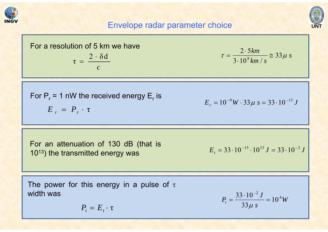
=For a resolution of 5 km we have
cdδ2τ ⋅
=
For an attenuation of 130 dB (that is 1013) the transmitted energy was JJEt
21315 1033101033 −− ⋅=⋅⋅=
JsWEr159 10333310 −− ⋅=⋅= μ
For Pr = 1 nW the received energy Er is
τ⋅= rr PE
Ws
JPt4
2
1033
1033=
⋅=
−
μ
The power for this energy in a pulse of τwidth was
τ⋅= tt EP
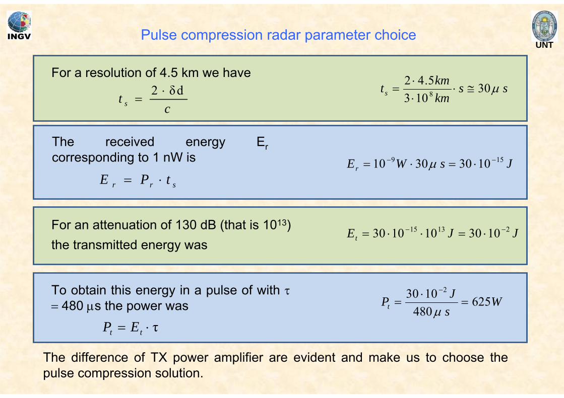
UNTPulse compression radar parameter choice
srr tPE ⋅=
The received energy Ercorresponding to 1 nW is JsWEr
159 10303010 −− ⋅=⋅= μ
For an attenuation of 130 dB (that is 1013) the transmitted energy was
JJEt21315 1030101030 −− ⋅=⋅⋅=
The difference of TX power amplifier are evident and make us to choose the pulse compression solution.
For a resolution of 4.5 km we havess
kmkmts μ30
1035.428 ≅⋅
⋅⋅
=
ct s
dδ2 ⋅=
To obtain this energy in a pulse of with τ = 480 μs the power was W
sJPt 625
4801030 2
=⋅
=−
μτ⋅= tt EP
UNT
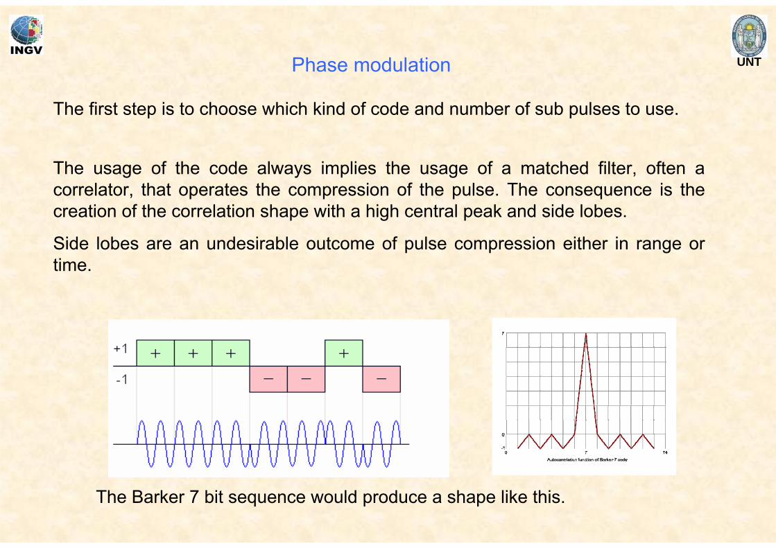
The first step is to choose which kind of code and number of sub pulses to use.
The usage of the code always implies the usage of a matched filter, often a correlator, that operates the compression of the pulse. The consequence is the creation of the correlation shape with a high central peak and side lobes.
Side lobes are an undesirable outcome of pulse compression either in range or time.
Phase modulation
The Barker 7 bit sequence would produce a shape like this.
UNT
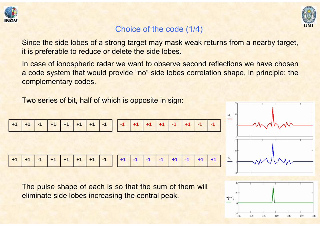
In case of ionospheric radar we want to observe second reflections we have chosen a code system that would provide “no” side lobes correlation shape, in principle: the complementary codes.
Since the side lobes of a strong target may mask weak returns from a nearby target, it is preferable to reduce or delete the side lobes.
Choice of the code (1/4)
+1 +1 -1 +1 +1 +1 +1 -1
+1 +1 -1 +1 +1 +1 +1 -1
-1 +1 +1 +1 -1 +1 -1 -1
+1 -1 -1 -1 +1 -1 +1 +1
Two series of bit, half of which is opposite in sign:
The pulse shape of each is so that the sum of them will eliminate side lobes increasing the central peak.
UNT
Considering that the targets are ionospheric layers and that can be considered steady the use of complementary codes is possible.
The complementary codes give the maximum effect of cancelling the side lobes when the phases of the echo are constant: they need to be referred to the same target.
The usage of such a solution would have been forbidden for airborne radars (for instance for glaciers survey).
Choice of the code (2/4)
UNT
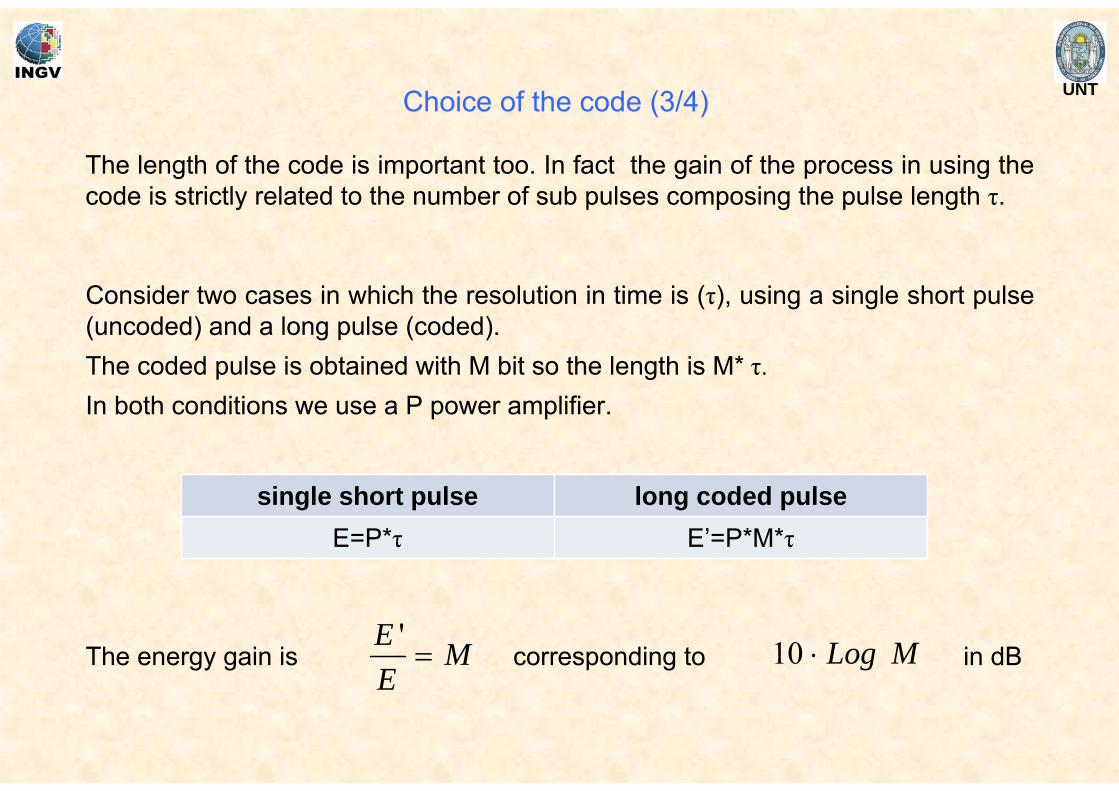
The length of the code is important too. In fact the gain of the process in using the code is strictly related to the number of sub pulses composing the pulse length τ.
Consider two cases in which the resolution in time is (τ), using a single short pulse (uncoded) and a long pulse (coded).The coded pulse is obtained with M bit so the length is M* τ.In both conditions we use a P power amplifier.
single short pulse long coded pulseE=P*τ E’=P*M*τ
The energy gain is MEE
=' MLog⋅10corresponding to in dB
Choice of the code (3/4)
UNT
According to Golay’s theory complementary couples of all length are possible but:short sequences give less gain but are fast to be processed;long sequences give high gain at the price of long processing time
Long sequences are not suitable for fast varying targets; in the ionospheric radars a frequent choice is to use 16 sub pulses complementary couple.
Choice of the code (4/4)
UNT
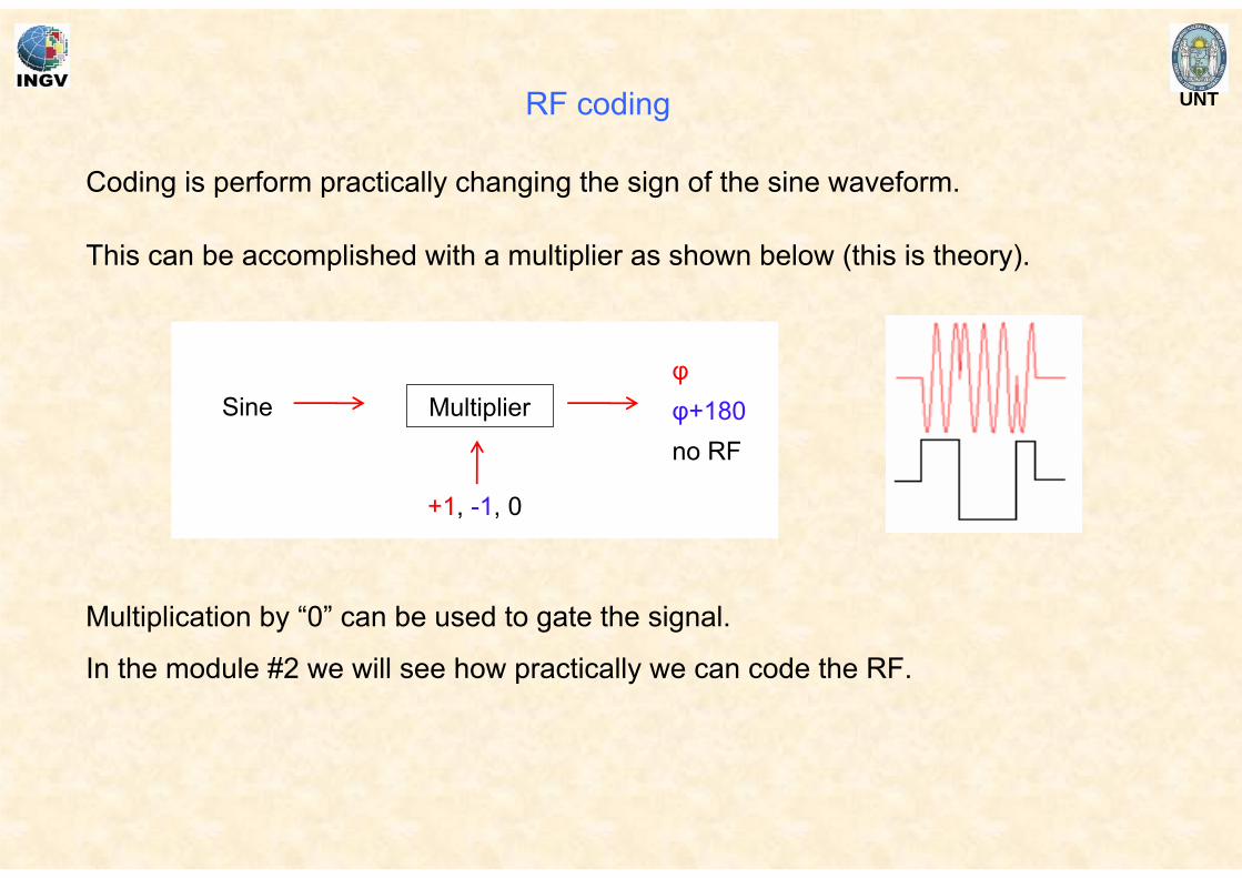
Coding is perform practically changing the sign of the sine waveform.
Multiplication by “0” can be used to gate the signal.
In the module #2 we will see how practically we can code the RF.
RF coding
This can be accomplished with a multiplier as shown below (this is theory).
Sine
+1, -1, 0
φφ+180no RF
Multiplier
UNT
The band pass of the signal is about 66 kHz useful to design the receiving stages.
Remembering that:the TX pulse width τ has to be < 600 μs (due to minimum distance); that ts should be around 33 μs (due to resolution);the complementary code 16 sub pulses is requested;the listening time is about 5 ms;
our final choice is ts =30 μs,number of bit=16τ = 480 μs (16 * ts)T < 200 Hz
Final choices
UNT
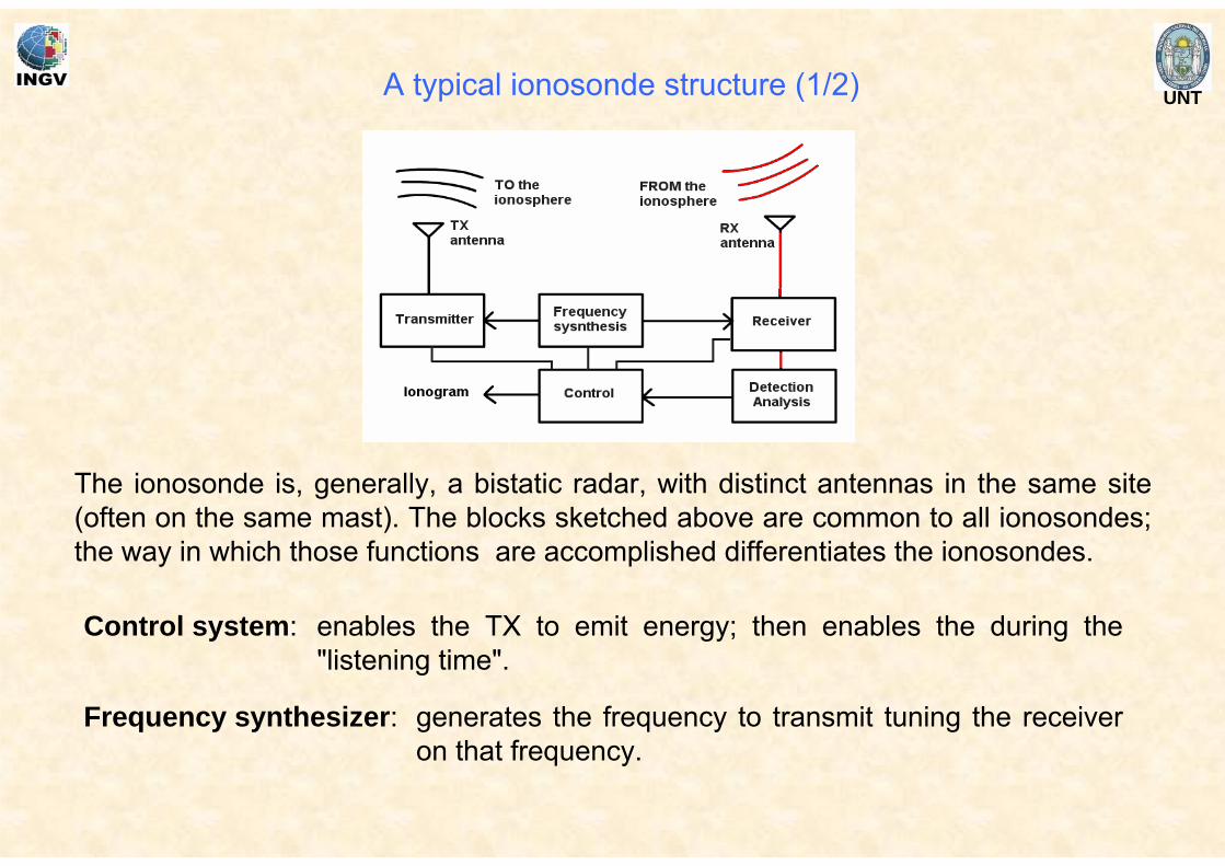
The ionosonde is, generally, a bistatic radar, with distinct antennas in the same site (often on the same mast). The blocks sketched above are common to all ionosondes; the way in which those functions are accomplished differentiates the ionosondes.
A typical ionosonde structure (1/2)
Control system: enables the TX to emit energy; then enables the during the "listening time".
Frequency synthesizer: generates the frequency to transmit tuning the receiver on that frequency.
UNT
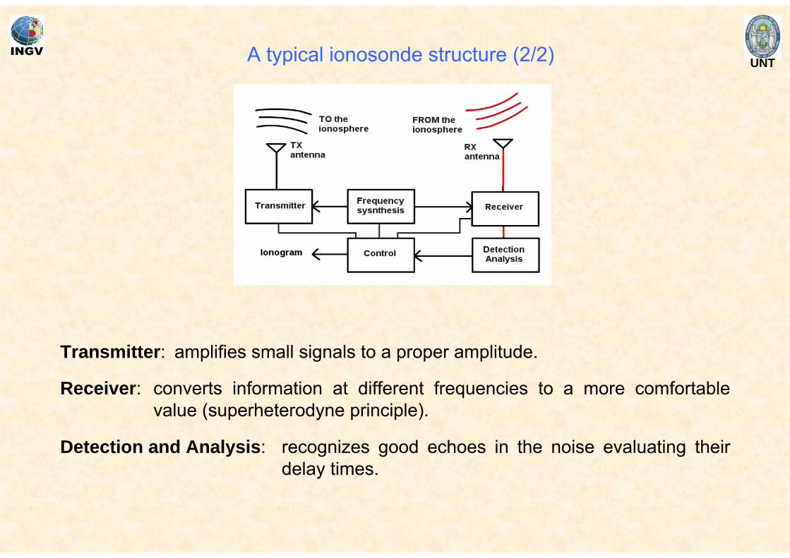
Transmitter: amplifies small signals to a proper amplitude.
Receiver: converts information at different frequencies to a more comfortable value (superheterodyne principle).
Detection and Analysis: recognizes good echoes in the noise evaluating their delay times.
A typical ionosonde structure (2/2)
UNT
2N steps
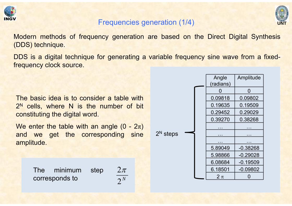
Frequencies generation (1/4)
Angle(radians)
Amplitude
0 00.09818 0.098020.19635 0.195090.29452 0.290290.39270 0.38268
… …… …… …
5.89049 -0.382685.98866 -0.290286.08684 -0.195096.18501 -0.09802
2 π 0
Modern methods of frequency generation are based on the Direct Digital Synthesis (DDS) technique.
DDS is a digital technique for generating a variable frequency sine wave from a fixed-frequency clock source.
The basic idea is to consider a table with 2N cells, where N is the number of bit constituting the digital word.
We enter the table with an angle (0 - 2π) and we get the corresponding sine amplitude.
The minimum step corresponds to N2
2π
UNT
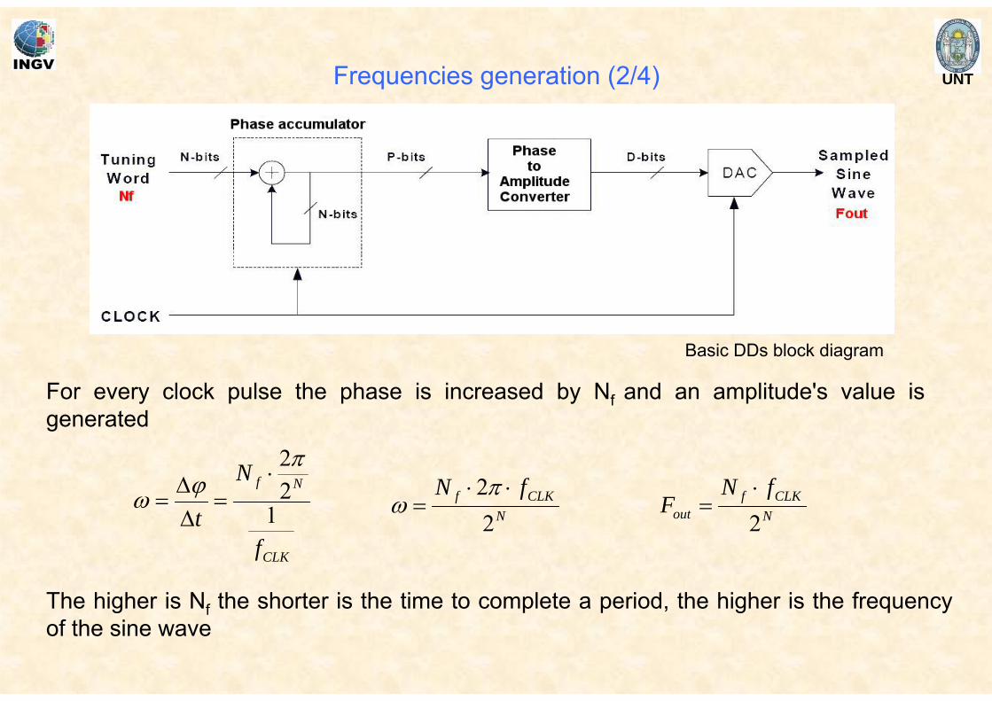
For every clock pulse the phase is increased by Nf and an amplitude's value is generated
Basic DDs block diagram
CLK
Nf
f
N
t 122π
ϕω⋅
=ΔΔ
=
The higher is Nf the shorter is the time to complete a period, the higher is the frequency of the sine wave
NCLKf fN
22 ⋅⋅
=π
ω NCLKf
out
fNF
2⋅
=
Frequencies generation (2/4)
UNT
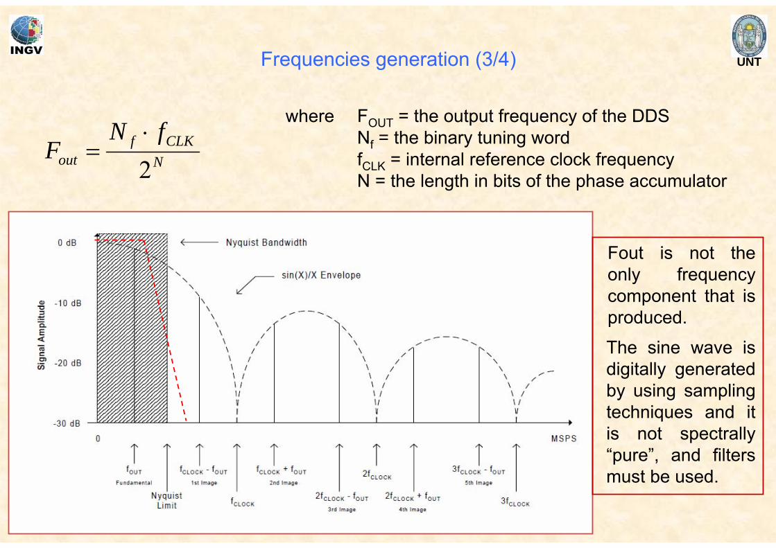
where FOUT = the output frequency of the DDSNf = the binary tuning wordfCLK = internal reference clock frequencyN = the length in bits of the phase accumulator
NCLKf
out
fNF
2⋅
=
Fout is not the only frequency component that is produced.
The sine wave is digitally generated by using sampling techniques and it is not spectrally “pure”, and filters must be used.
Frequencies generation (3/4)
UNT
FREQUENCY digitally tunable (typically with sub-Hertz resolution).
PHASE is digitally adjustable, as well,
NO ERRORS from drift due to temperature or aging of components.
Two generators from the same clock will have phase locked frequency.
FREQUENCY must be less than or equal to 1/2 the clock source frequency.
The sine wave AMPLITUDE is generally fixed.
The sine wave is not spectrally “pure”, and filters must be used.
DDS advantages
DDS restrictions
Frequencies generation (4/4)
UNTFrequency conversion
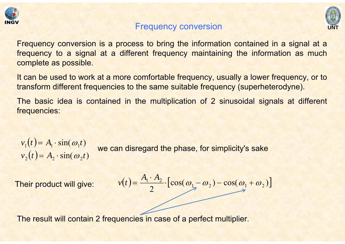
Frequency conversion is a process to bring the information contained in a signal at a frequency to a signal at a different frequency maintaining the information as much complete as possible.
It can be used to work at a more comfortable frequency, usually a lower frequency, or to transform different frequencies to the same suitable frequency (superheterodyne).
The basic idea is contained in the multiplication of 2 sinusoidal signals at different frequencies:
we can disregard the phase, for simplicity's sake ( )( ) )sin(
)sin(
222
111
tAtvtAtv
ωω
⋅=⋅=
Their product will give: ( ) [ ])cos()cos(2 2121
21 ωωωω +−−⋅⋅
=AAtv
The result will contain 2 frequencies in case of a perfect multiplier.
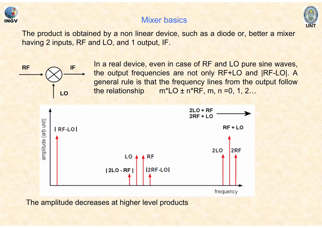
UNTThe product is obtained by a non linear device, such as a diode or, better a mixer having 2 inputs, RF and LO, and 1 output, IF.
In a real device, even in case of RF and LO pure sine waves, the output frequencies are not only RF+LO and |RF-LO|. A general rule is that the frequency lines from the output follow the relationship m*LO ± n*RF, m, n =0, 1, 2…
RF IF
LO
The amplitude decreases at higher level products
Mixer basics
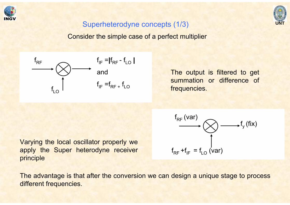
UNT
fRF
fLO
fIF =|fRF - fLO |
and
fIF =fRF + fLO
The output is filtered to get summation or difference of frequencies.
fRF (var)
fRF +fIF = fLO (var)
fy (fix)
Varying the local oscillator properly we apply the Super heterodyne receiver principle
Superheterodyne concepts (1/3)
The advantage is that after the conversion we can design a unique stage to process different frequencies.
Consider the simple case of a perfect multiplier
UNT
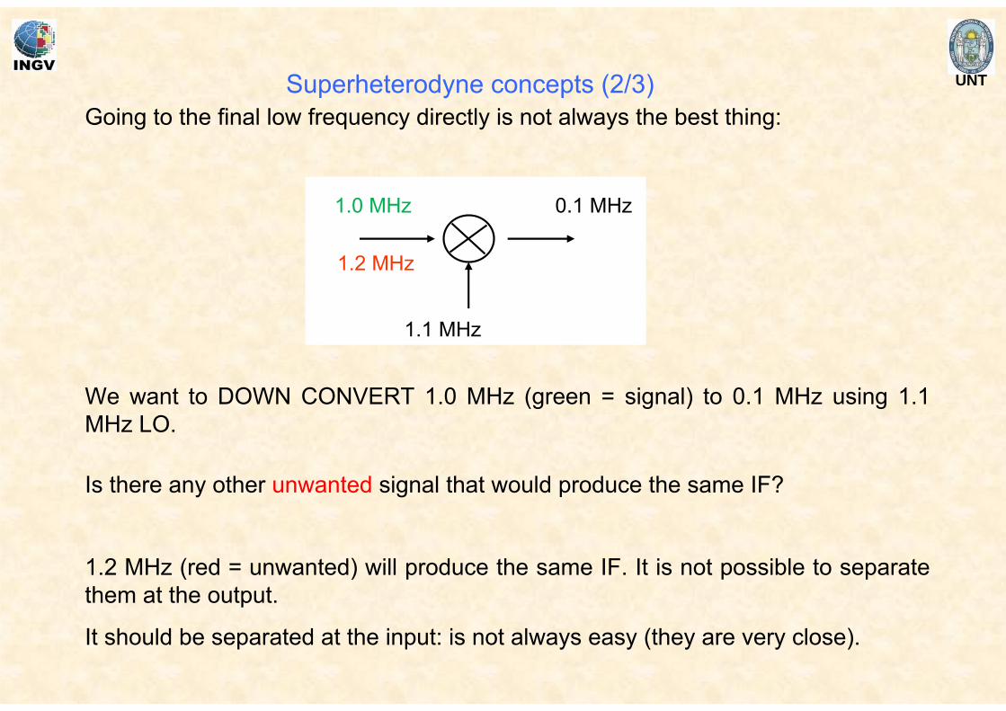
Going to the final low frequency directly is not always the best thing:
1.0 MHz
1.1 MHz
0.1 MHz
We want to DOWN CONVERT 1.0 MHz (green = signal) to 0.1 MHz using 1.1 MHz LO.
Is there any other unwanted signal that would produce the same IF?
1.2 MHz (red = unwanted) will produce the same IF. It is not possible to separate them at the output.
It should be separated at the input: is not always easy (they are very close).
?1.2 MHz
Superheterodyne concepts (2/3)
UNT
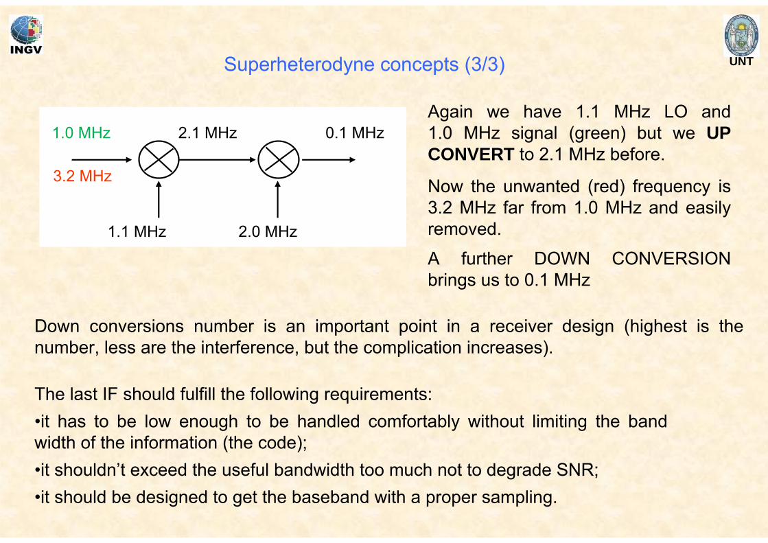
Down conversions number is an important point in a receiver design (highest is the number, less are the interference, but the complication increases).
Again we have 1.1 MHz LO and 1.0 MHz signal (green) but we UP CONVERT to 2.1 MHz before.
Now the unwanted (red) frequency is 3.2 MHz far from 1.0 MHz and easily removed.
1.0 MHz
1.1 MHz
2.1 MHz
3.2 MHz
2.0 MHz
0.1 MHz
A further DOWN CONVERSION brings us to 0.1 MHz
The last IF should fulfill the following requirements:•it has to be low enough to be handled comfortably without limiting the band width of the information (the code);•it shouldn’t exceed the useful bandwidth too much not to degrade SNR;•it should be designed to get the baseband with a proper sampling.
Superheterodyne concepts (3/3)
UNT
Antennas for vertical ionospheric sounding are a crucial element in the general design.
The following requirements should be satisfied for both TX and RX antennas:
• they have to be wide band to accept the wide frequency range (a simple dipole is
not allowed due to its resonance);
• the main radiation lobe needs to be directed upwards;
• they need to have a good gain because the ionospheric attenuation and the
geometrical loss reduce greatly the signal amplitude.
Antennas for vertical ionospheric sounding
UNT
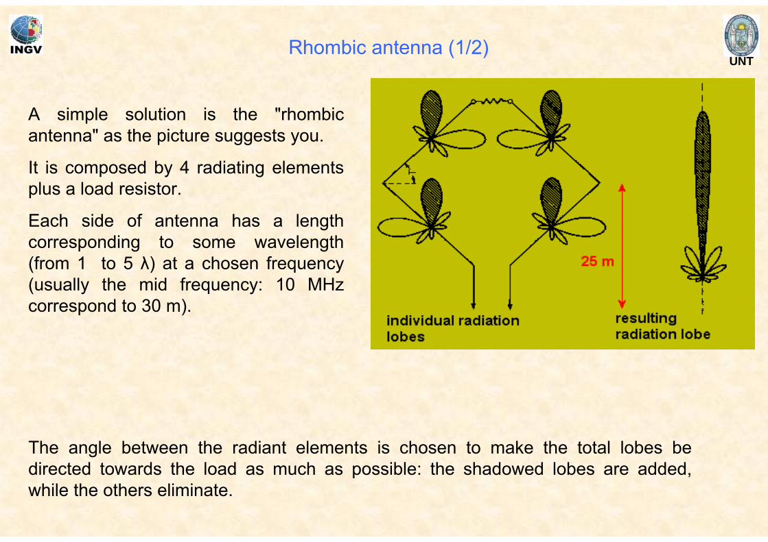
A simple solution is the "rhombic antenna" as the picture suggests you.
It is composed by 4 radiating elements plus a load resistor.
Each side of antenna has a length corresponding to some wavelength (from 1 to 5 λ) at a chosen frequency (usually the mid frequency: 10 MHz correspond to 30 m).
The angle between the radiant elements is chosen to make the total lobes be directed towards the load as much as possible: the shadowed lobes are added, while the others eliminate.
Rhombic antenna (1/2)
UNT
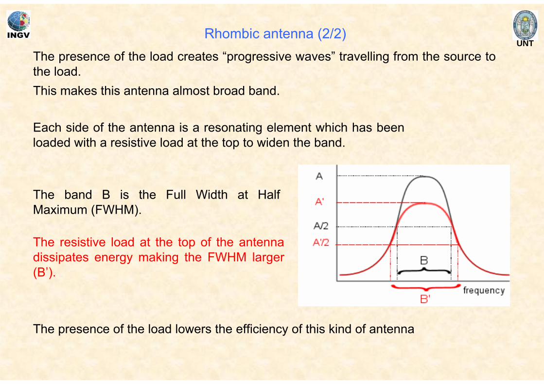
Each side of the antenna is a resonating element which has been loaded with a resistive load at the top to widen the band.
The band B is the Full Width at Half Maximum (FWHM).
The resistive load at the top of the antenna dissipates energy making the FWHM larger (B’).
The presence of the load creates “progressive waves” travelling from the source to the load.This makes this antenna almost broad band.
The presence of the load lowers the efficiency of this kind of antenna
Rhombic antenna (2/2)
UNTDelta antenna (1/2)
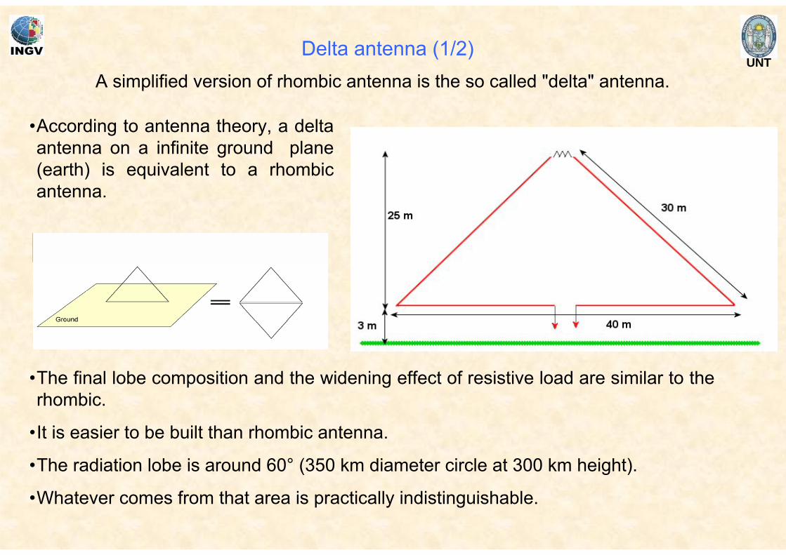
A simplified version of rhombic antenna is the so called "delta" antenna.
•According to antenna theory, a delta antenna on a infinite ground plane (earth) is equivalent to a rhombic antenna.
•The final lobe composition and the widening effect of resistive load are similar to the rhombic.
•It is easier to be built than rhombic antenna.
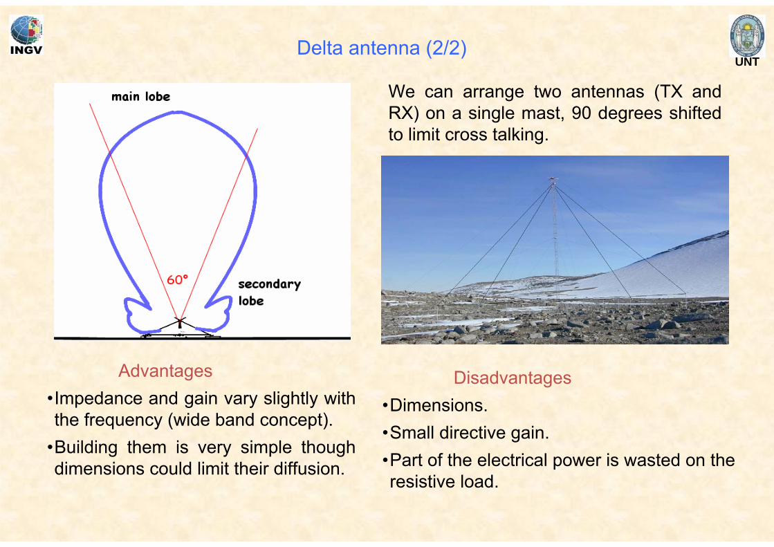
•The radiation lobe is around 60° (350 km diameter circle at 300 km height).
•Whatever comes from that area is practically indistinguishable.
UNT
Advantages•Impedance and gain vary slightly with the frequency (wide band concept).
•Building them is very simple though dimensions could limit their diffusion.
Disadvantages•Dimensions.•Small directive gain.•Part of the electrical power is wasted on the resistive load.
We can arrange two antennas (TX and RX) on a single mast, 90 degrees shifted to limit cross talking.
Delta antenna (2/2)
UNTBalun (1/3)
In rhombic antenna or in delta one we have to transfer energy from and to antenna
facing two problems:
•to go from unbalanced signal (ground referenced) to symmetric lines (balanced);
•to transfer energy between two objects with different impedances.
Matching of the impedance is important to optimize the energy transfer without
damaging the amplifier in TX line, and not to waste the very few energy in RX
chain.
This double task is realized with special transformers called balun. Baluns are
devices connecting BALanced terminals to UNbalanced ones.
UNT
Matching of the impedance cannot be realized exactly for all frequency range (we
are dealing with real devices!!!) but it is possible to reach good compromises.
p
s
p
s
RR
NN
=⎟⎟⎠
⎞⎜⎜⎝
⎛2
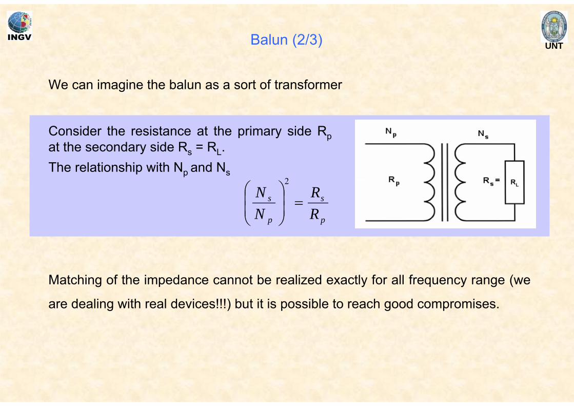
Consider the resistance at the primary side Rpat the secondary side Rs = RL.The relationship with Np and Ns
We can imagine the balun as a sort of transformer
Balun (2/3)
UNT
There are a lot of possible schemes that can be applied (it is a sort of art) depending on the antenna type and the particular application.Considering the frequencies at which we work the material we use is another important detail.
Very high magnetic permeability gives high efficiency in energy transfer.
Considering the very few losses we desire, toroids of high permeability alloys are used, like permalloy.
Balun (3/3)

UNTSignal processing: introduction
We can assume that the signal processing starts after the last IF. The following operations are aimed to keep the information as much complete as possible and are:
•to sample IF during the listening time usually getting phase and quadrature channels. The amplitude is the amplitude of the phasor (kind of vector);
•to apply the proper procedures to find the code (use of matched filter);
•to use proper algorithms to increase SNR to make the detection safer (filtering, integration);
•to give to the targets a spatial position related to the delay of the echoes.
In analog old ionosondes most of the previous operations are performed in a hardware mode (matched filters, integrations) but in modern digital system all of them are accomplished in a numerical way.
UNTADC sampling
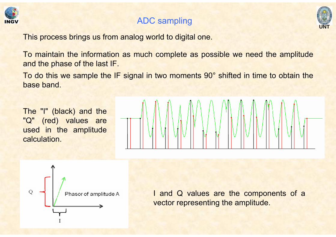
This process brings us from analog world to digital one.
To maintain the information as much complete as possible we need the amplitude and the phase of the last IF.To do this we sample the IF signal in two moments 90° shifted in time to obtain the base band.
The "I" (black) and the "Q" (red) values are used in the amplitude calculation.
I and Q values are the components of a vector representing the amplitude.
UNT
I
Q
A
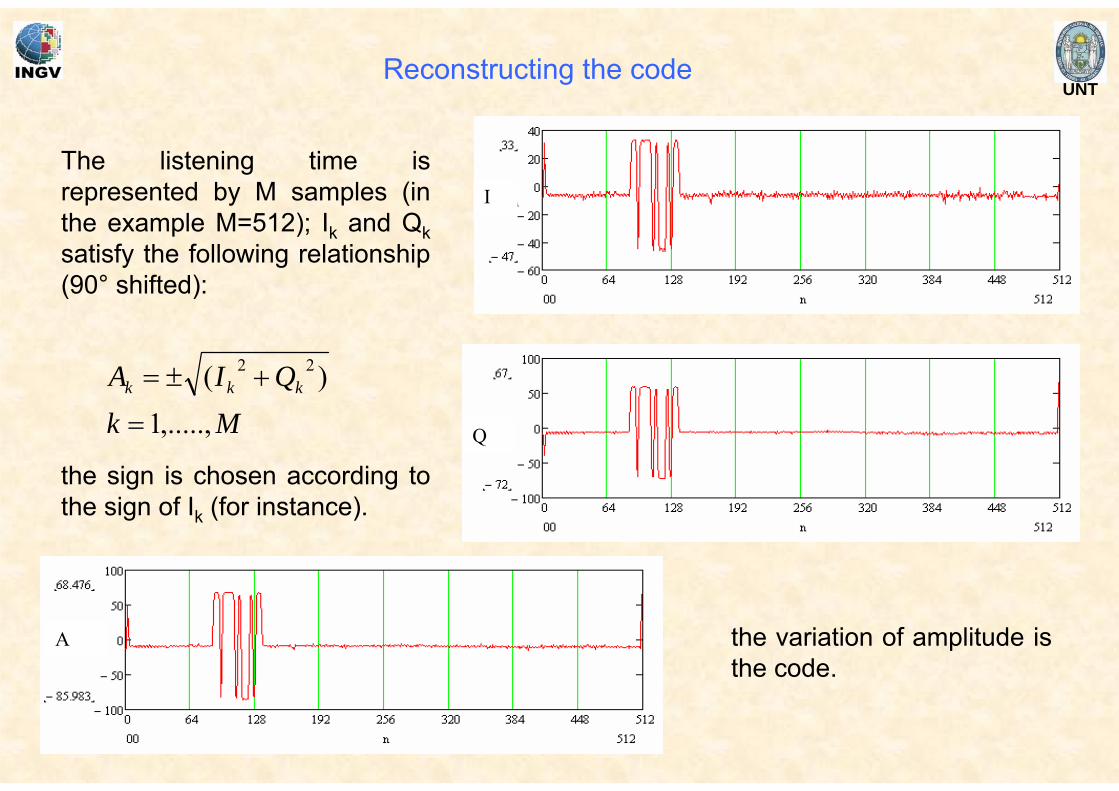
The listening time is represented by M samples (in the example M=512); Ik and Qksatisfy the following relationship (90° shifted):
MkQIA kkk
,.....,1)( 22
=
+±=
the variation of amplitude is the code.
the sign is chosen according to the sign of Ik (for instance).
Reconstructing the code
UNTMatched filter (1/2)
The previous example showed a quasi ideal case, in which noise is almost zero
and the code is easily visible.
In the general case we need a method to detect the presence of the code and to
evaluate the delay time.
This subject can be considered as a special case of filter and convolution theory:
the problem of finding a short template signal inside a long time series.
The idea is to use a filter that is able to maximize SNR when the template is
detected; such a filter is called a matched filter.
UNT
The matched filter is the optimal linear filter for maximizing SNR in the presence
of additive stochastic noise. It works convolving the unknown signal (received
signal) with a conjugated time-reversed version of the template (CODE).
Practically this is equivalent to correlate the template, with the unknown signal to
detect the presence of the code.
The correlation operation can be executed both in time domain and in frequency
domain, where the operation is simpler, because it is achieved by simply
multiplying the spectra. In the following we will discuss only the time domain
operations.
Matched filter (2/2)
UNTCorrelation
⊗
=
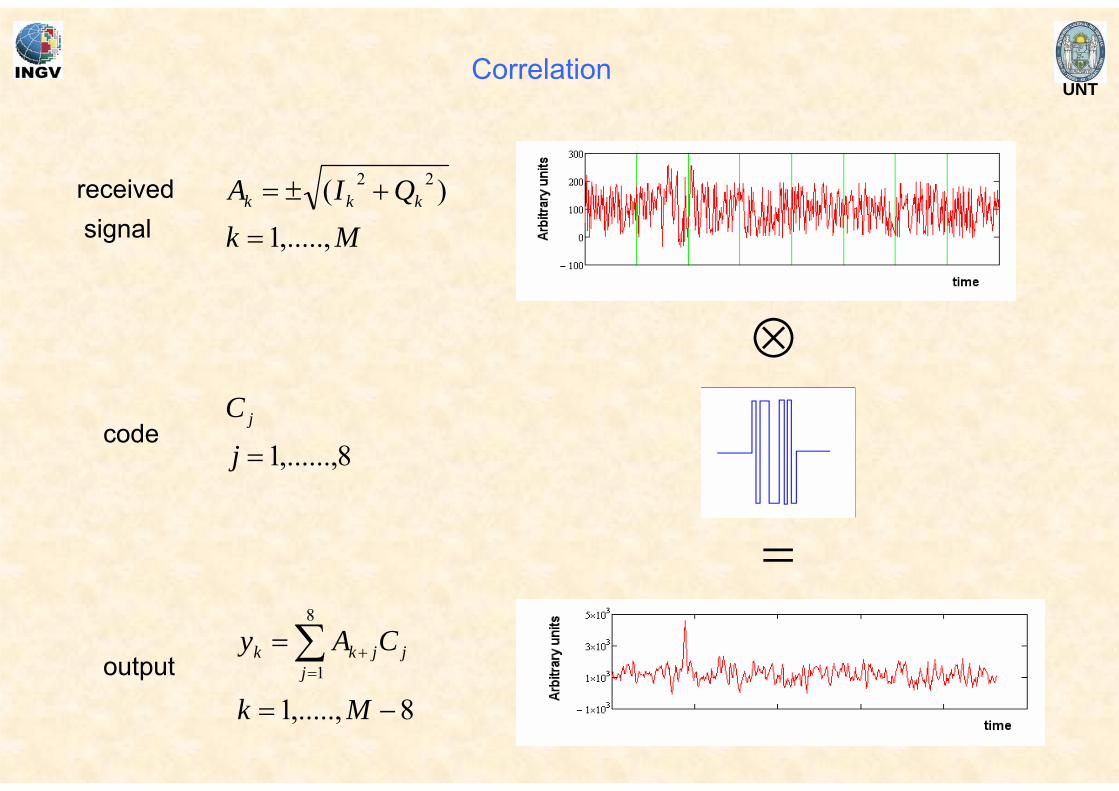
receivedsignal
code
output
MkQIA kkk
,.....,1)( 22
=
+±=
8,.....,1
8
1
−=
= ∑=
+
Mk
CAyj
jjkk
8,......,1=j
C j
UNT
In the radar technique we can distinguish between COHERENT and
INCOHERENT integration related to the moment at which we perform the
summation of the pulses contribution:
COHERENT we integrate before the detection, that is when the
phase of each pulse is still available and usable;
NON COHERENT the integration is performed after the detection.
Integration
Except very rare case of a extremely good SNR a single pulse is not enough to
allow the proper and safe detection of a target.
So we usually use the integration technique to increase the SNR and to get a
good Pd.
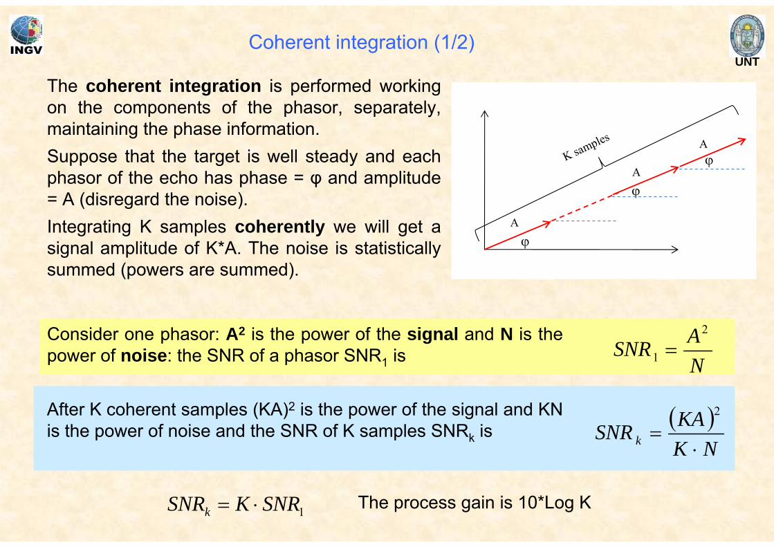
UNTCoherent integration (1/2)
The coherent integration is performed working on the components of the phasor, separately, maintaining the phase information.Suppose that the target is well steady and each phasor of the echo has phase = φ and amplitude = A (disregard the noise).Integrating K samples coherently we will get a signal amplitude of K*A. The noise is statistically summed (powers are summed).
ϕ
ϕ
ϕK samples
A
A
A
The process gain is 10*Log K
NASNR
2
1 =Consider one phasor: A2 is the power of the signal and N is the power of noise: the SNR of a phasor SNR1 is
( )NK
KASNR k ⋅=
2After K coherent samples (KA)2 is the power of the signal and KN is the power of noise and the SNR of K samples SNRk is
1SNRKSNRk ⋅=
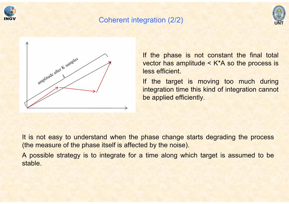
UNT
If the phase is not constant the final total vector has amplitude < K*A so the process is less efficient.If the target is moving too much during integration time this kind of integration cannot be applied efficiently.
It is not easy to understand when the phase change starts degrading the process (the measure of the phase itself is affected by the noise).A possible strategy is to integrate for a time along which target is assumed to be stable.
amplitude after K
samples
Coherent integration (2/2)
UNT
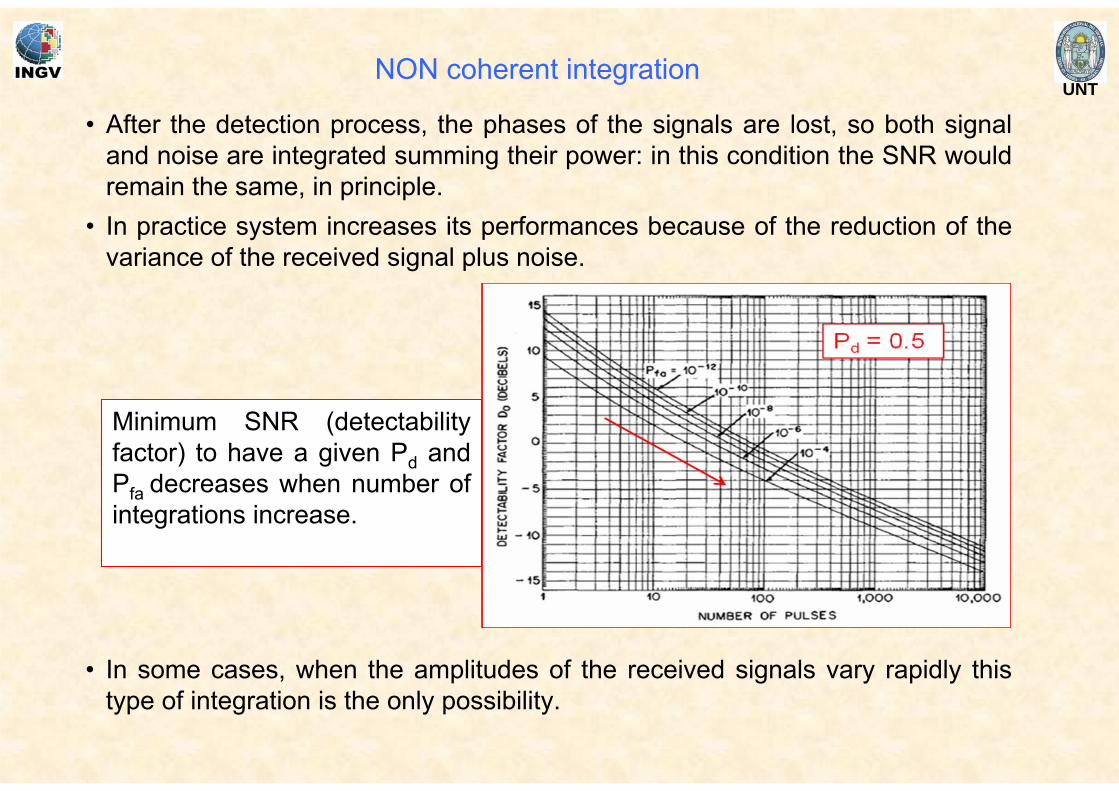
• After the detection process, the phases of the signals are lost, so both signal and noise are integrated summing their power: in this condition the SNR would remain the same, in principle.
• In practice system increases its performances because of the reduction of the variance of the received signal plus noise.
NON coherent integration
• In some cases, when the amplitudes of the received signals vary rapidly this type of integration is the only possibility.
Minimum SNR (detectabilityfactor) to have a given Pd and Pfa decreases when number of integrations increase.
UNTDetection
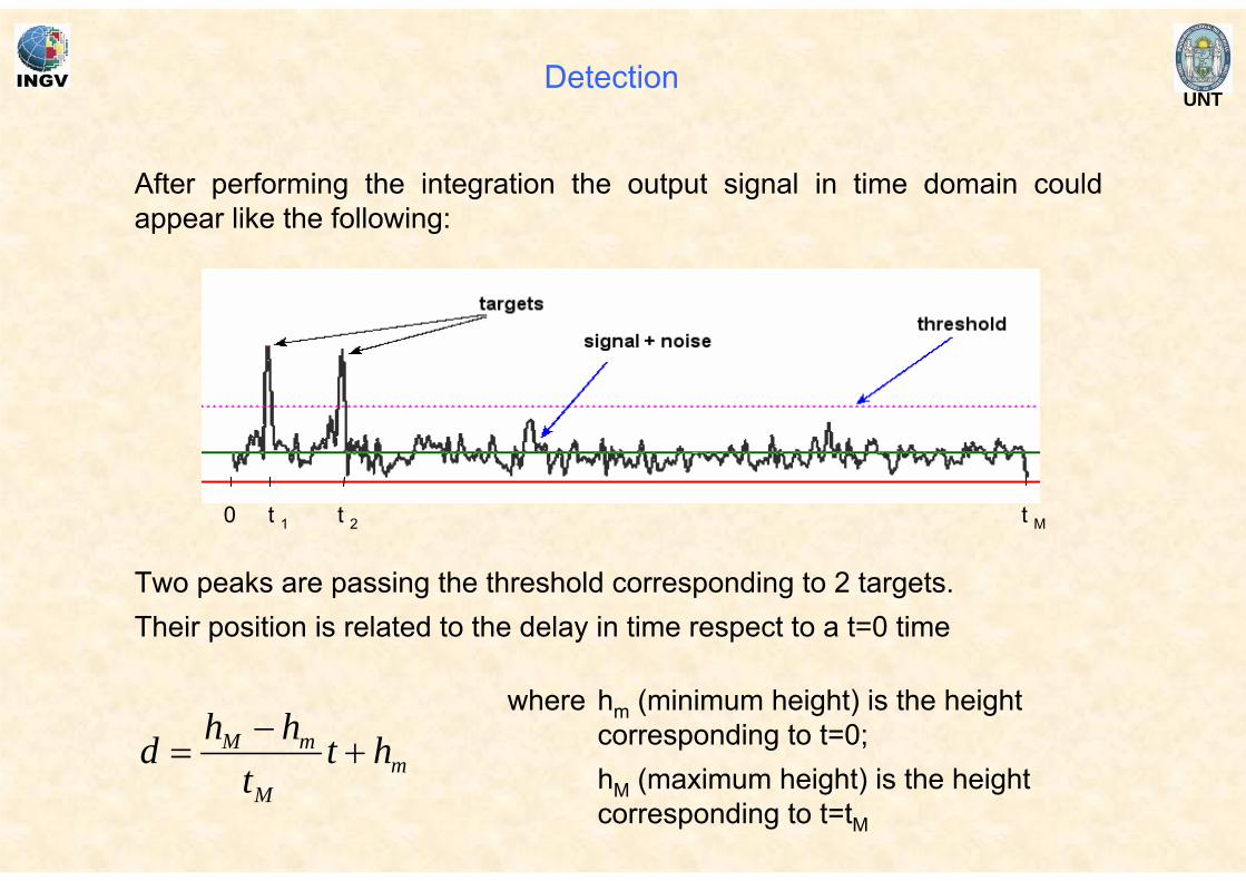
After performing the integration the output signal in time domain could appear like the following:
Two peaks are passing the threshold corresponding to 2 targets.Their position is related to the delay in time respect to a t=0 time
0 t 1 t 2 t M
mM
mM htt
hhd +−
=where hm (minimum height) is the height
corresponding to t=0;hM (maximum height) is the height corresponding to t=tM
UNT
After the modulus calculation we have to determine the cited threshold,
exceeding which any return can be considered to probably originate from a layer.
Threshold low: more targets will be detected, increasing numbers of
false alarms too.
Threshold high: fewer targets will be detected, and the number of
false alarms will also be small.
We cannot use a fixed threshold because the noise level changes in time during
the sounding. A changing threshold can be used, where the threshold level is
raised and lowered to maintain a constant probability of false alarm. This is
known as constant false alarm rate (CFAR) detection.
Determining the threshold
UNT
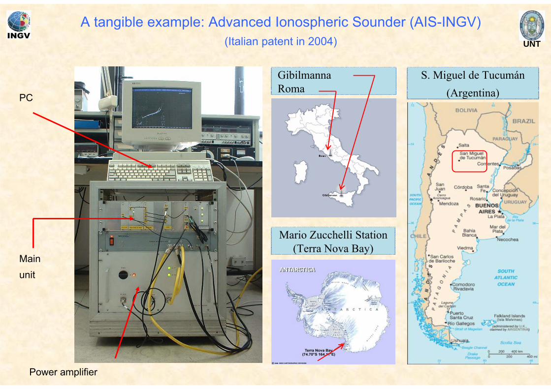
A tangible example: Advanced Ionospheric Sounder (AIS-INGV)(Italian patent in 2004)
GibilmannaRoma
Mario Zucchelli Station (Terra Nova Bay)
S. Miguel de Tucumán(Argentina)
Mainunit
Power amplifier
PC
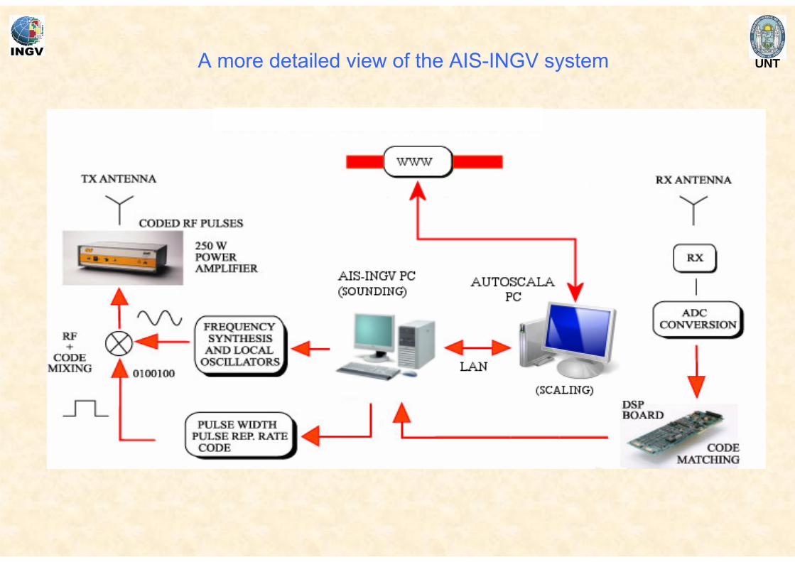
UNTA more detailed view of the AIS-INGV system
UNT
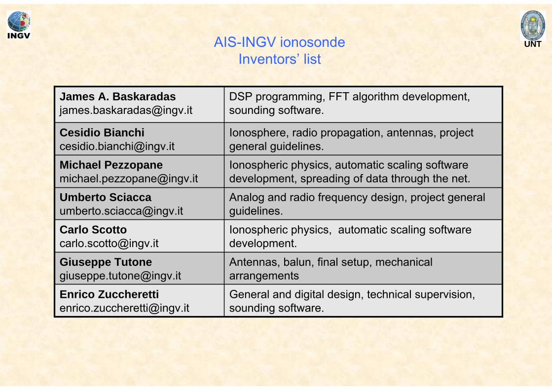
General and digital design, technical supervision, sounding software.
Enrico [email protected]
Antennas, balun, final setup, mechanical arrangements
Giuseppe [email protected]
Ionospheric physics, automatic scaling software development.
Carlo [email protected]
Analog and radio frequency design, project general guidelines.
Umberto [email protected]
Ionospheric physics, automatic scaling software development, spreading of data through the net.
Michael [email protected]
Ionosphere, radio propagation, antennas, project general guidelines.
Cesidio [email protected]
DSP programming, FFT algorithm development, sounding software.
James A. [email protected]
AIS-INGV ionosondeInventors’ list
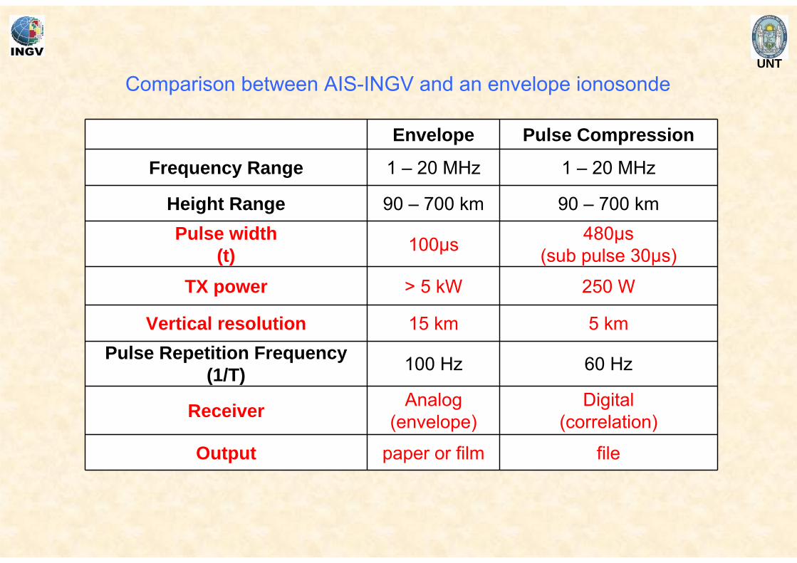
UNT
Envelope Pulse Compression
Frequency Range 1 – 20 MHz 1 – 20 MHz
Height Range 90 – 700 km 90 – 700 kmPulse width
(t) 100μs 480μs(sub pulse 30μs)
TX power > 5 kW 250 W
Vertical resolution 15 km 5 kmPulse Repetition Frequency
(1/T) 100 Hz 60 Hz
Receiver Analog(envelope)
Digital(correlation)
Output paper or film file
Comparison between AIS-INGV and an envelope ionosonde
UNT
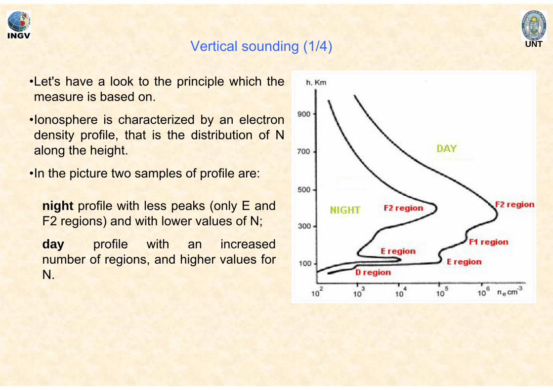
•Let's have a look to the principle which the measure is based on.
•Ionosphere is characterized by an electron density profile, that is the distribution of N along the height.
•In the picture two samples of profile are:
Vertical sounding (1/4)
night profile with less peaks (only E and F2 regions) and with lower values of N;
day profile with an increased number of regions, and higher values for N.
UNT
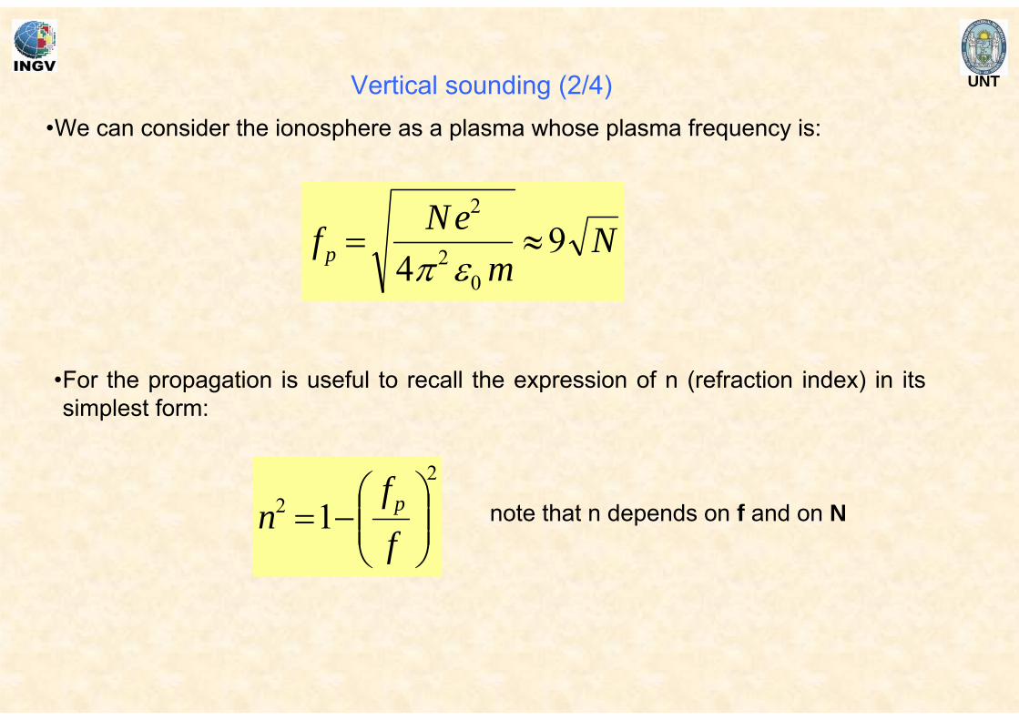
•We can consider the ionosphere as a plasma whose plasma frequency is:
Nm
eNfp 94 0
2
2
≈=επ
•For the propagation is useful to recall the expression of n (refraction index) in its simplest form:
22 1 ⎟⎟
⎠
⎞⎜⎜⎝
⎛−=
ff
n p note that n depends on f and on N
Vertical sounding (2/4)
UNT
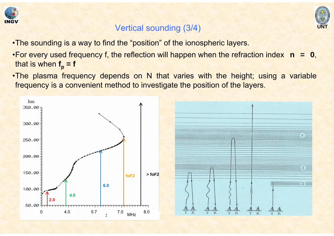
•The sounding is a way to find the “position” of the ionospheric layers.•For every used frequency f, the reflection will happen when the refraction index n = 0, that is when fp = f
•The plasma frequency depends on N that varies with the height; using a variable frequency is a convenient method to investigate the position of the layers.
1011 electrons / m3MHz0 4.0 5.7 7.0 8.0
2.04.0
6.0
foF2 > foF2
Vertical sounding (3/4)
UNT
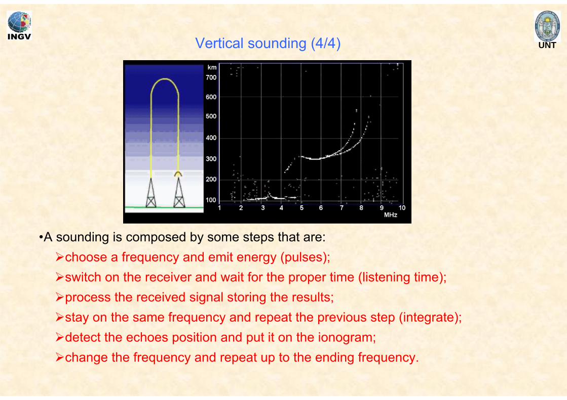
•A sounding is composed by some steps that are:choose a frequency and emit energy (pulses);switch on the receiver and wait for the proper time (listening time);process the received signal storing the results;stay on the same frequency and repeat the previous step (integrate);detect the echoes position and put it on the ionogram;change the frequency and repeat up to the ending frequency.
Vertical sounding (4/4)
UNT
Frequency limits: fmin ≥ 1.5 MHz (broad casting, anthropic noise)fmax depends on the site, the season, the solar cycle.
Frequency step: from 50 kHz to 100 kHz (rarely 25 kHz).(frequency resolution)
Time integration: from fractions of seconds up to few seconds.
Sounding duration: can last from few seconds to 2 - 3 minutes .
Soundings scheduling: depends on sounding application; routine manually scaled every hour;routine automatically scaled every 15 min;special campaign every 5 min.
Planning a sounding
Whatever ionosonde is used some parameters need to be decided to plan a sounding
UNT
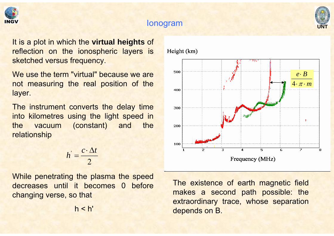
It is a plot in which the virtual heights of reflection on the ionospheric layers is sketched versus frequency.
We use the term "virtual" because we are not measuring the real position of the layer.
The instrument converts the delay time into kilometres using the light speed in the vacuum (constant) and the relationship
While penetrating the plasma the speed decreases until it becomes 0 before changing verse, so that
h < h'
The existence of earth magnetic field makes a second path possible: the extraordinary trace, whose separation depends on B.
Ionogram
2' tch Δ⋅=
mBe⋅⋅
⋅π4
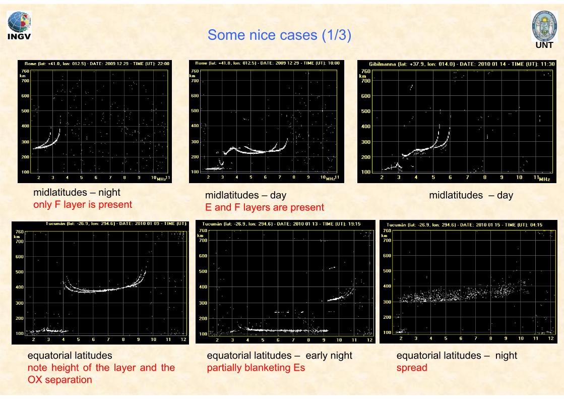
UNTSome nice cases (1/3)
midlatitudes – nightonly F layer is present
midlatitudes – daymidlatitudes – dayE and F layers are present
equatorial latitudes – nightspread
equatorial latitudes – early nightpartially blanketing Es
equatorial latitudesnote height of the layer and the OX separation
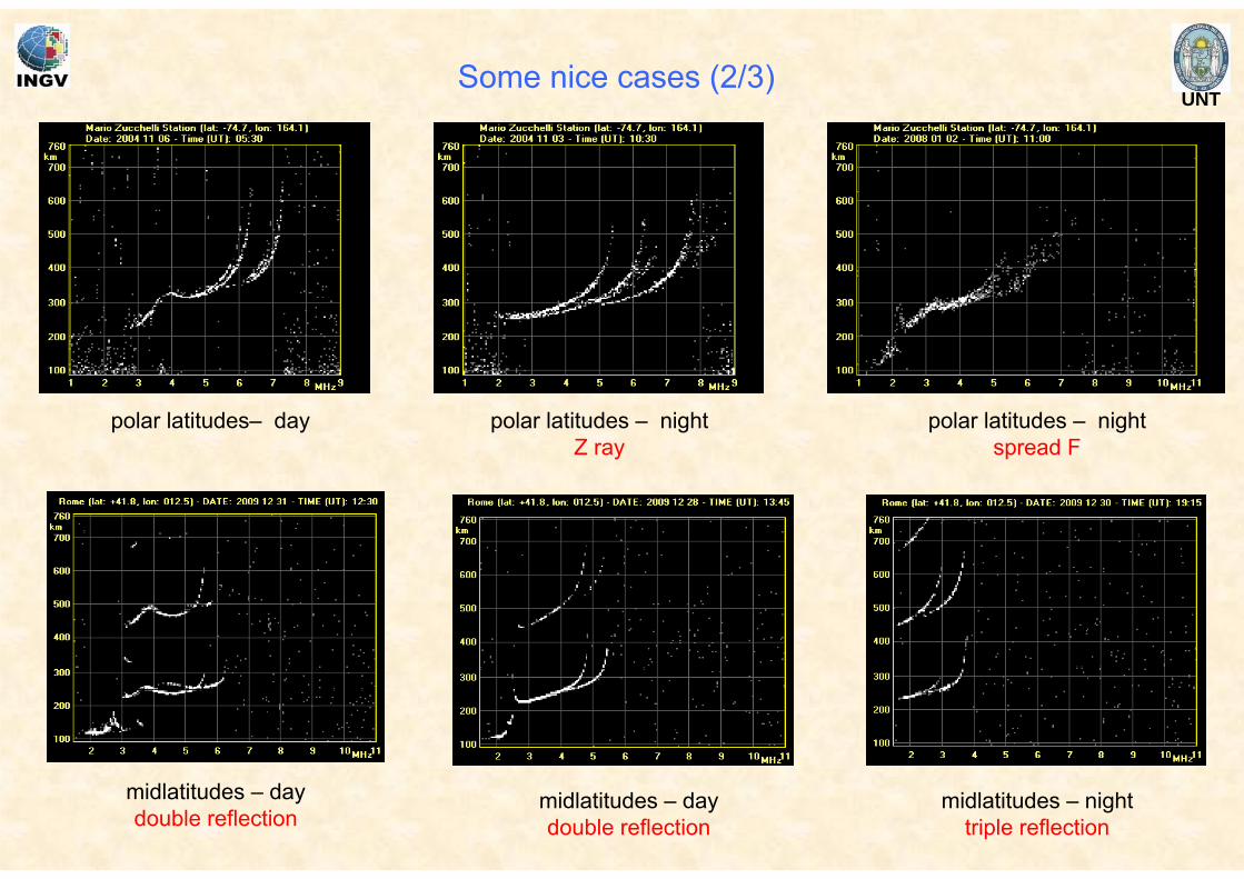
UNT
midlatitudes – daydouble reflection
midlatitudes – nighttriple reflection
midlatitudes – daydouble reflection
polar latitudes– day polar latitudes – nightZ ray
polar latitudes – nightspread F
Some nice cases (2/3)
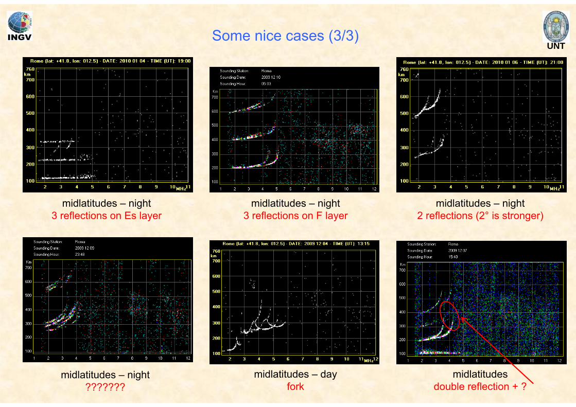
UNT
midlatitudes – night3 reflections on Es layer
midlatitudes – night3 reflections on F layer
midlatitudes – night2 reflections (2° is stronger)
midlatitudes – dayfork
midlatitudes – night???????
midlatitudesdouble reflection + ?
Some nice cases (3/3)
UNT
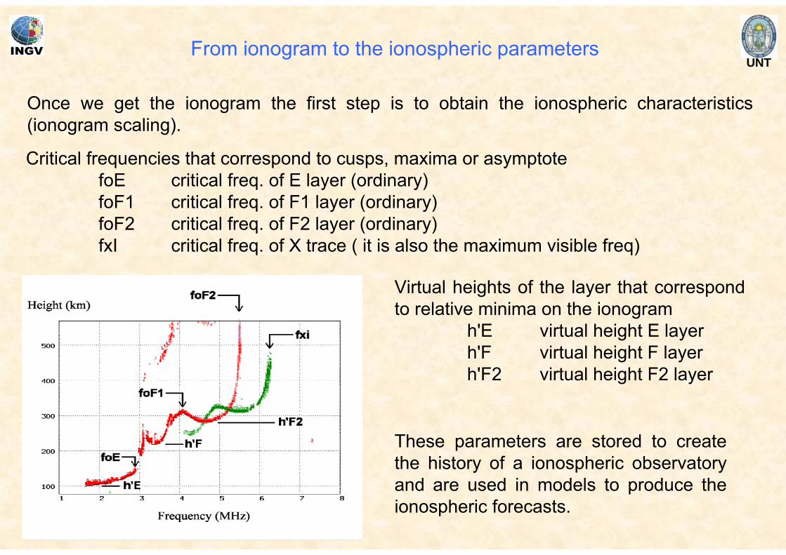
Once we get the ionogram the first step is to obtain the ionospheric characteristics (ionogram scaling).
Critical frequencies that correspond to cusps, maxima or asymptotefoE critical freq. of E layer (ordinary)foF1 critical freq. of F1 layer (ordinary)foF2 critical freq. of F2 layer (ordinary)fxI critical freq. of X trace ( it is also the maximum visible freq)
These parameters are stored to create the history of a ionospheric observatory and are used in models to produce the ionospheric forecasts.
From ionogram to the ionospheric parameters
Virtual heights of the layer that correspond to relative minima on the ionogram
h'E virtual height E layerh'F virtual height F layerh'F2 virtual height F2 layer
UNTFrom ionogram to the density profile
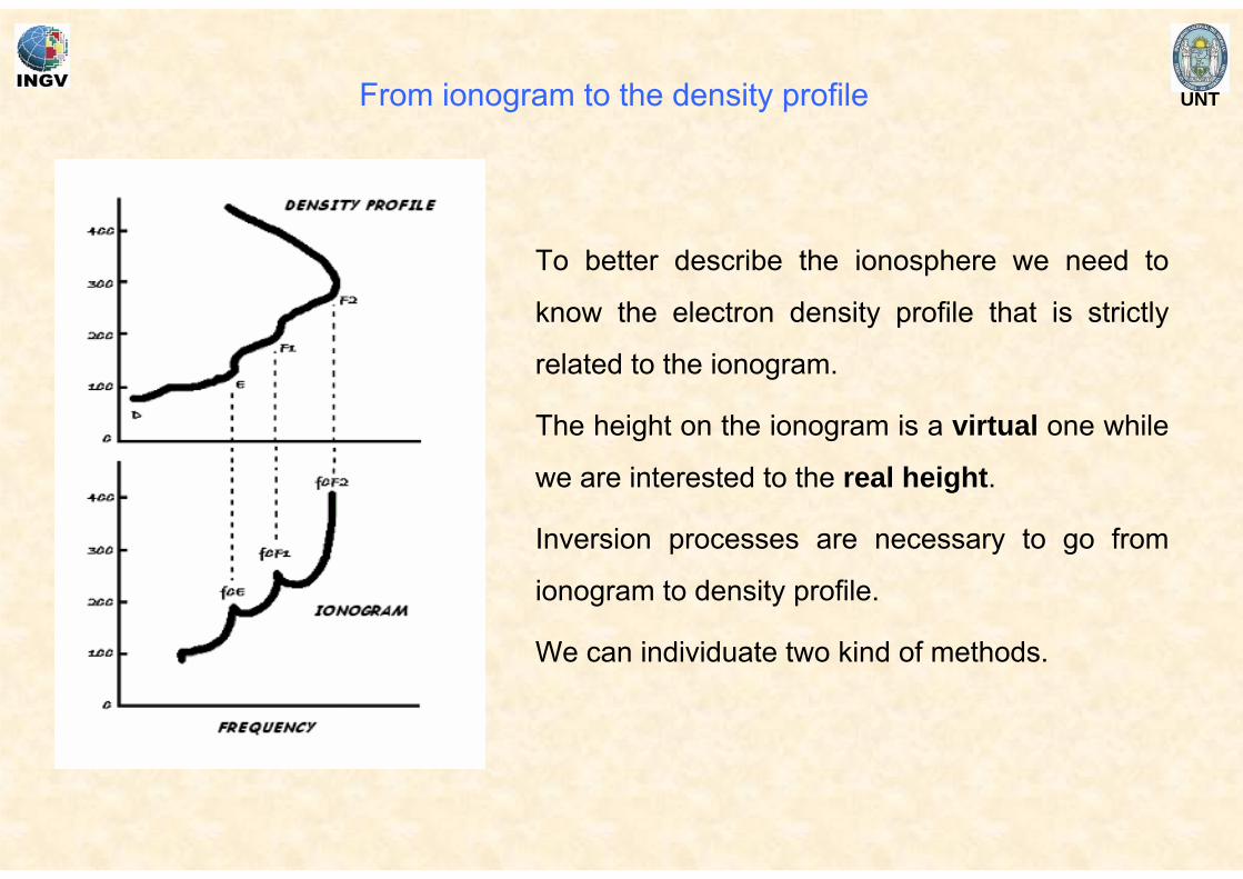
To better describe the ionosphere we need to
know the electron density profile that is strictly
related to the ionogram.
The height on the ionogram is a virtual one while
we are interested to the real height.
Inversion processes are necessary to go from
ionogram to density profile.
We can individuate two kind of methods.
UNT
• We generate a starting density profile and a corresponding synthetic ionogram;• a comparison between it and the measured ionogram is performed;• the profile is varied in some convenient way producing another synthetic
ionogram to compare;• when the synthetic ionogram is similar (some criteria) to the measured one the
process ends giving the density profile.• This is a convenient method executable after a sounding.
Polynomial inversion method
• We start from the digitized ionogram considering it as (f, h’)couples. • There are models partially empirical able to describe analytically the different
ionospheric regions from helio - geophysical and ionospheric quantities (POLAN by Titheridge).
Successive approximation method
Possible methods
UNT
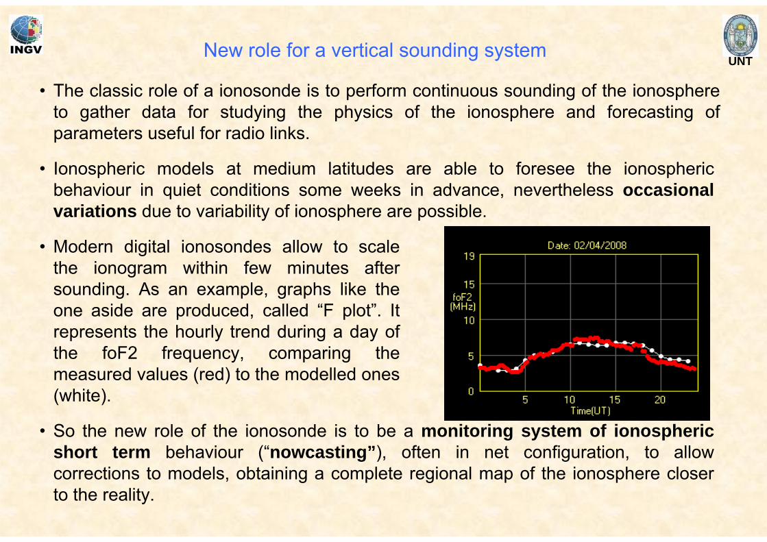
• The classic role of a ionosonde is to perform continuous sounding of the ionosphere to gather data for studying the physics of the ionosphere and forecasting of parameters useful for radio links.
New role for a vertical sounding system
• Ionospheric models at medium latitudes are able to foresee the ionospheric behaviour in quiet conditions some weeks in advance, nevertheless occasional variations due to variability of ionosphere are possible.
• So the new role of the ionosonde is to be a monitoring system of ionospheric short term behaviour (“nowcasting”), often in net configuration, to allow corrections to models, obtaining a complete regional map of the ionosphere closer to the reality.
• Modern digital ionosondes allow to scale the ionogram within few minutes after sounding. As an example, graphs like the one aside are produced, called “F plot”. It represents the hourly trend during a day of the foF2 frequency, comparing the measured values (red) to the modelled ones (white).
UNTHalloween storm at Gibilmanna (1/2)
2
4
6
8
10
12
14
16
0 1 2 3 4 5 6 7 8 9 10 11 12 13 14 15 16 17 18 19 20 21 22 23
long term valuesmeasured
2003 October 25
2
4
6
8
10
12
14
16
0 1 2 3 4 5 6 7 8 9 10 11 12 13 14 15 16 17 18 19 20 21 22 23
long term valuesmeasured
2003 October 26
2
4
6
8
10
12
14
16
0 1 2 3 4 5 6 7 8 9 10 11 12 13 14 15 16 17 18 19 20 21 22 23
long term valuesmeasured
2003 October 27
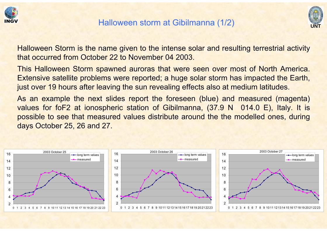
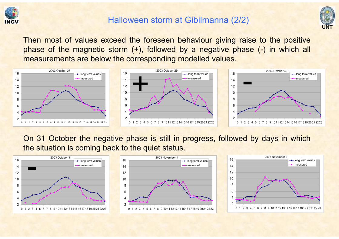
Halloween Storm is the name given to the intense solar and resulting terrestrial activity that occurred from October 22 to November 04 2003.This Halloween Storm spawned auroras that were seen over most of North America. Extensive satellite problems were reported; a huge solar storm has impacted the Earth, just over 19 hours after leaving the sun revealing effects also at medium latitudes.As an example the next slides report the foreseen (blue) and measured (magenta) values for foF2 at ionospheric station of Gibilmanna, (37.9 N 014.0 E), Italy. It is possible to see that measured values distribute around the the modelled ones, during days October 25, 26 and 27.
UNT
2
4
6
8
10
12
14
16
0 1 2 3 4 5 6 7 8 9 10 11 12 13 14 15 16 17 18 19 20 21 22 23
long term valuesmeasured
2003 October 28
2
4
6
8
10
12
14
16
0 1 2 3 4 5 6 7 8 9 10 11 12 13 14 15 16 17 18 19 20 21 22 23
long term valuesmeasured
2003 October 29
+2
4
6
8
10
12
14
16
0 1 2 3 4 5 6 7 8 9 10 11 12 13 14 15 16 17 18 19 20 21 22 23
long term valuesmeasured
2003 October 30-Then most of values exceed the foreseen behaviour giving raise to the positive phase of the magnetic storm (+), followed by a negative phase (-) in which all measurements are below the corresponding modelled values.
Halloween storm at Gibilmanna (2/2)
On 31 October the negative phase is still in progress, followed by days in which the situation is coming back to the quiet status.
2
4
6
8
10
12
14
16
0 1 2 3 4 5 6 7 8 9 10 11 12 13 14 15 16 17 18 19 20 21 22 23
long term valuesmeasured
2003 November 1
2
4
6
8
10
12
14
16
0 1 2 3 4 5 6 7 8 9 10 11 12 13 14 15 16 17 18 19 20 21 22 23
long term valuesmeasured
2003 November 2
2
4
6
8
10
12
14
16
0 1 2 3 4 5 6 7 8 9 10 11 12 13 14 15 16 17 18 19 20 21 22 23
long term valuesmeasured
2003 October 31-
UNT
•Barton D. K., Leonov S. A. (editors), Radar Technology Encyclopedia, Artech House Inc., 1998.
•Budden K.G., Radio wave in the ionosphere, Cambridge Univ. Press UK, 1966.
•Davies K., Ionospheric Radio, published as IEE Electromagnetic Waves Series No, 31 Peter Peregrinus Ltd London, UK, 1990.
•McNamara L. F., The ionosphere: communications, surveillance and direction finding, Krieger Publishing Company, 1991.
•Hunsucker R. D., Radio techniques for probing the terrestrial ionosphere, Springer-Verlag, 1991.
•Skolnik M., Radar handbook, Mc Graw Hill, 1990.
Bibliography
UNT
Module 2
The AIS-INGV and
Tucumán system
UNT
Mainunit
Power amplifier
PC
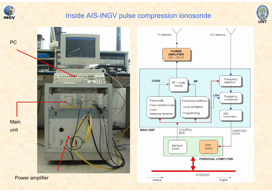
Inside AIS-INGV pulse compression ionosonde
UNT
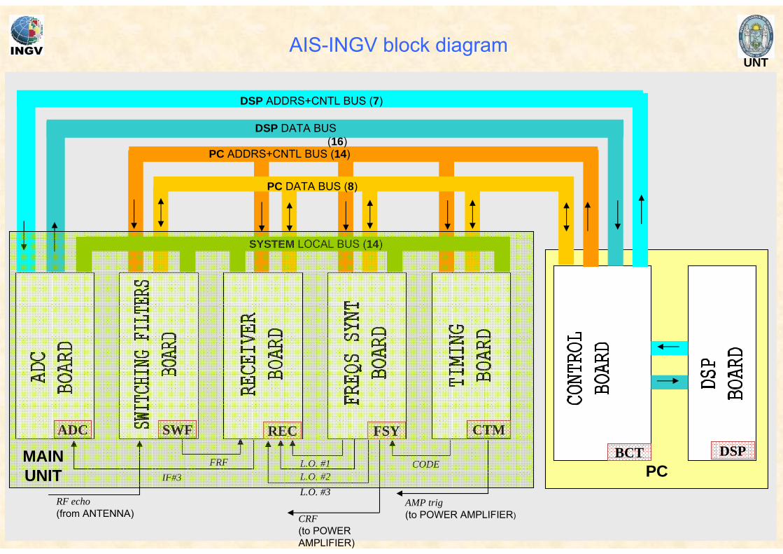
DSP ADDRS+CNTL BUS (7)
DSP DATA BUS(16)
PC ADDRS+CNTL BUS (14)
SYSTEM LOCAL BUS (14)
PC DATA BUS (8)
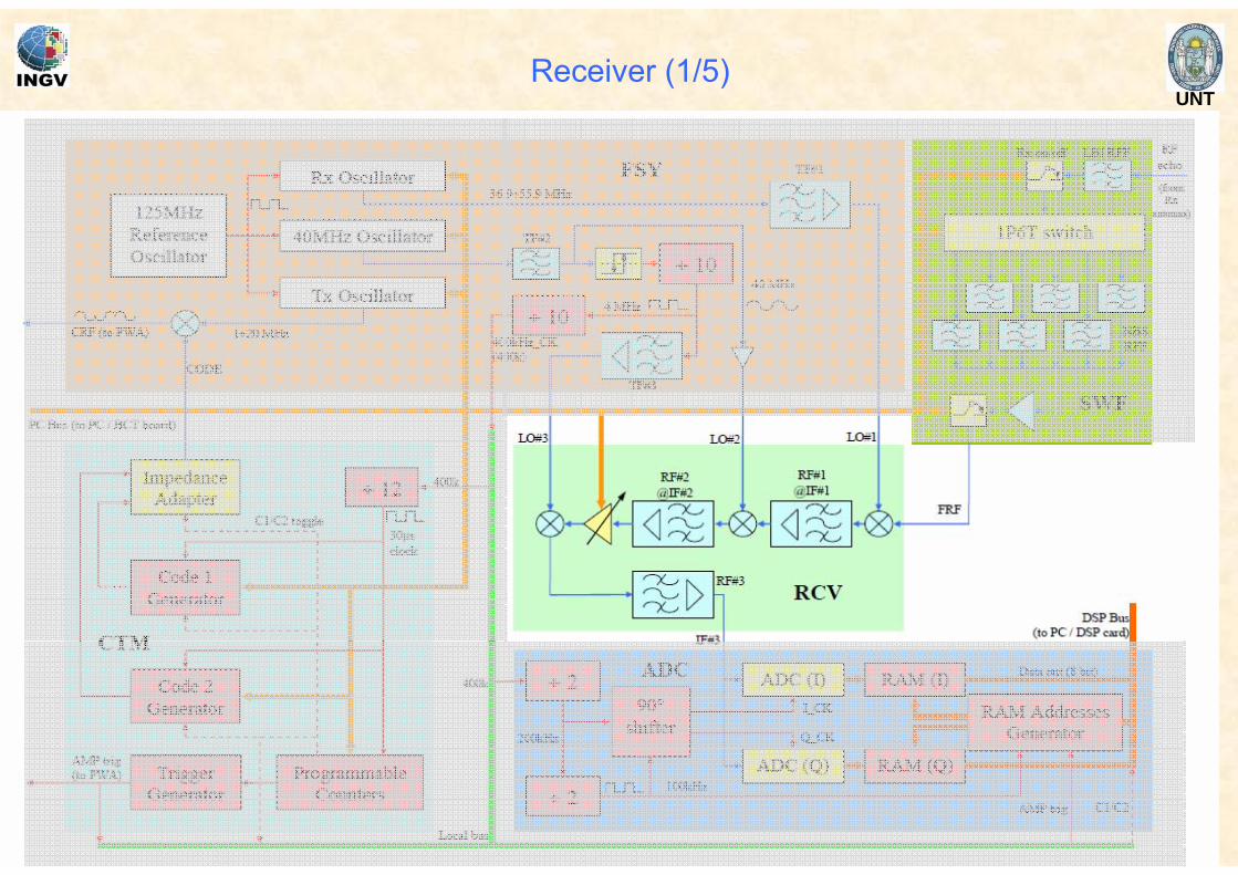
PCL.O. #1L.O. #2L.O. #3
CODEIF#3
RF echo(from ANTENNA) CRF
(to POWER AMPLIFIER)
AMP trig(to POWER AMPLIFIER)
FRF
FSY CTMRECSWFADCDSPBCT
AIS-INGV block diagram
MAIN UNIT
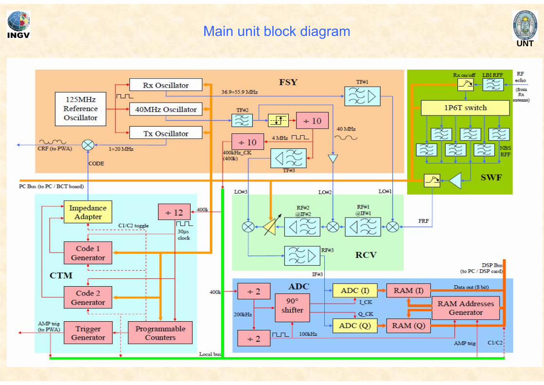
UNTMain unit block diagram
UNT
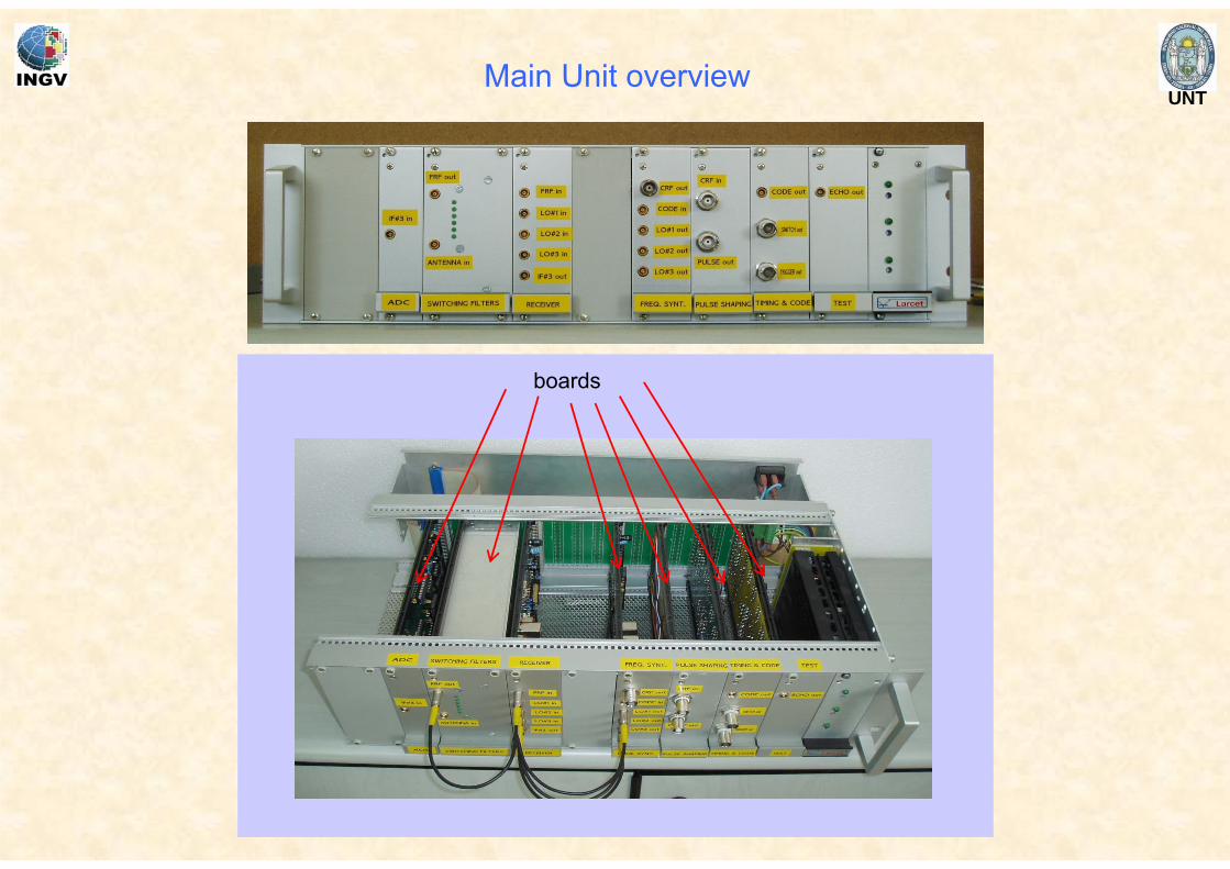
boards
Main Unit overview
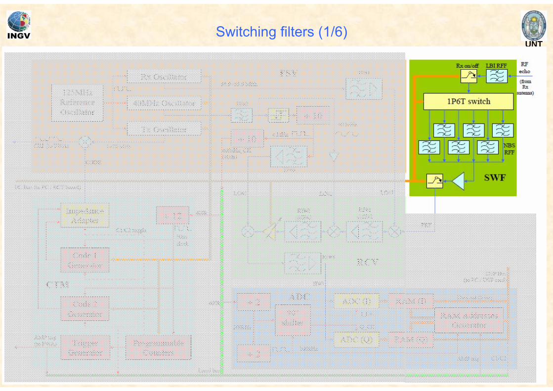
UNTSwitching filters (1/6)
UNT
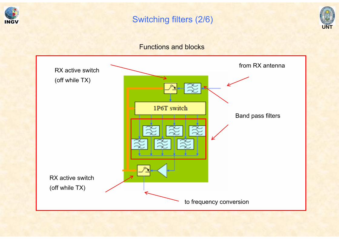
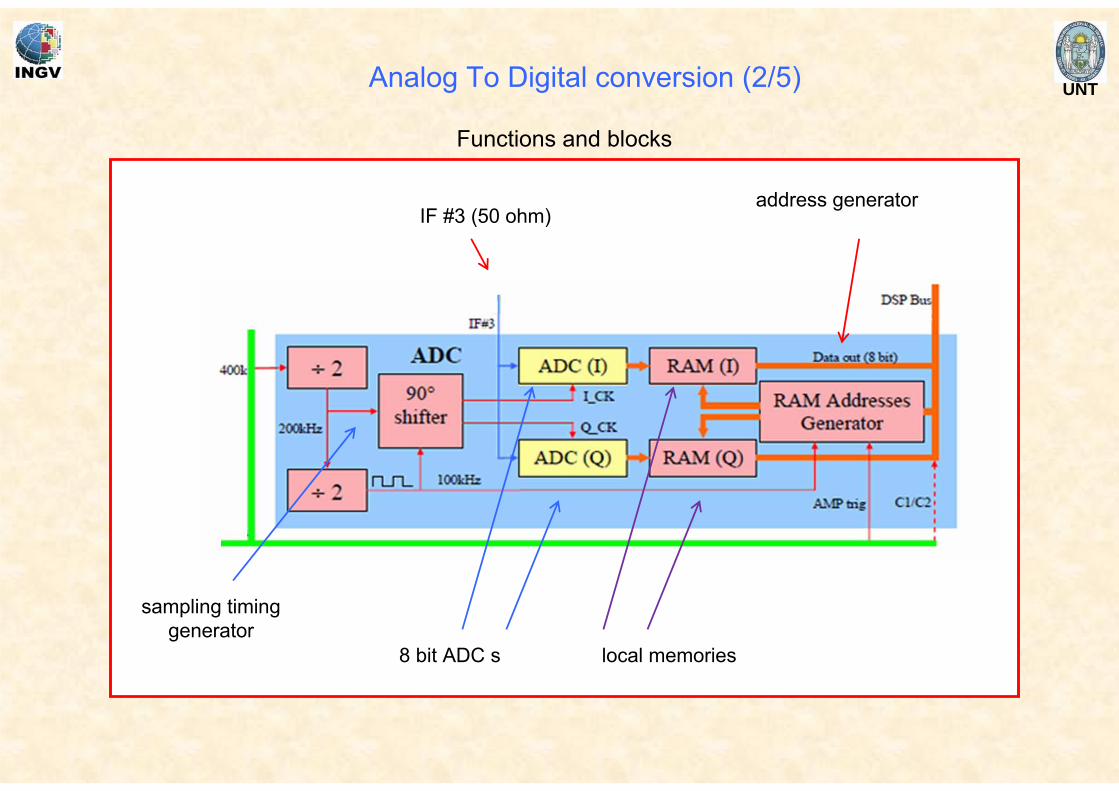
Functions and blocks
Band pass filters
RX active switch(off while TX)
RX active switch(off while TX)
from RX antenna
to frequency conversion
Switching filters (2/6)
UNT
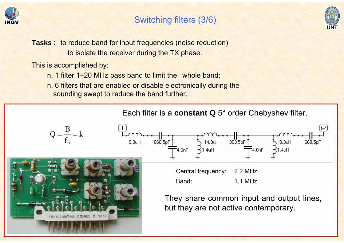
kfBQ
0
==
Central frequency: 2.2 MHz Band: 1.1 MHz
Each filter is a constant Q 5° order Chebyshev filter.
They share common input and output lines, but they are not active contemporary.
Tasks : to reduce band for input frequencies (noise reduction)to isolate the receiver during the TX phase.
This is accomplished by:n. 1 filter 1÷20 MHz pass band to limit the whole band;n. 6 filters that are enabled or disable electronically during the
sounding swept to reduce the band further.
Switching filters (3/6)
UNT
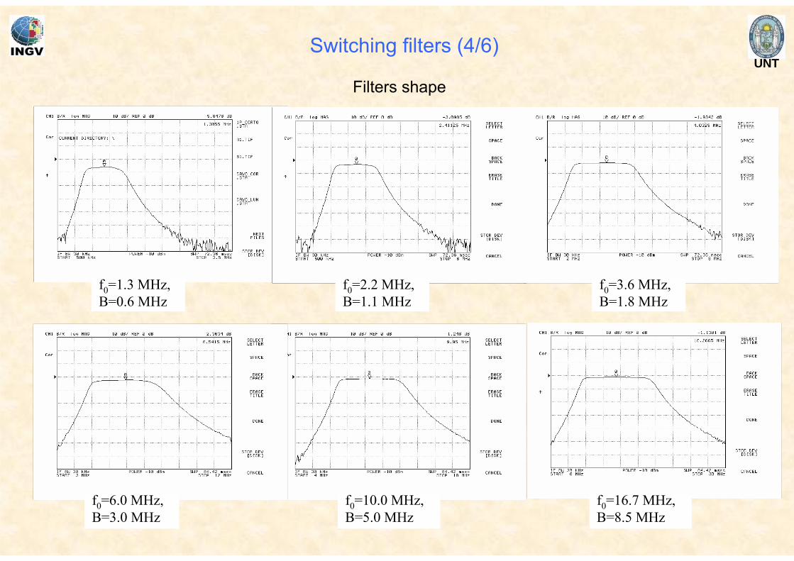
f0=1.3 MHz,B=0.6 MHz
f0=2.2 MHz,B=1.1 MHz
f0=3.6 MHz,B=1.8 MHz
f0=16.7 MHz,B=8.5 MHz
f0=10.0 MHz,B=5.0 MHz
f0=6.0 MHz,B=3.0 MHz
Filters shape
Switching filters (4/6)
UNT
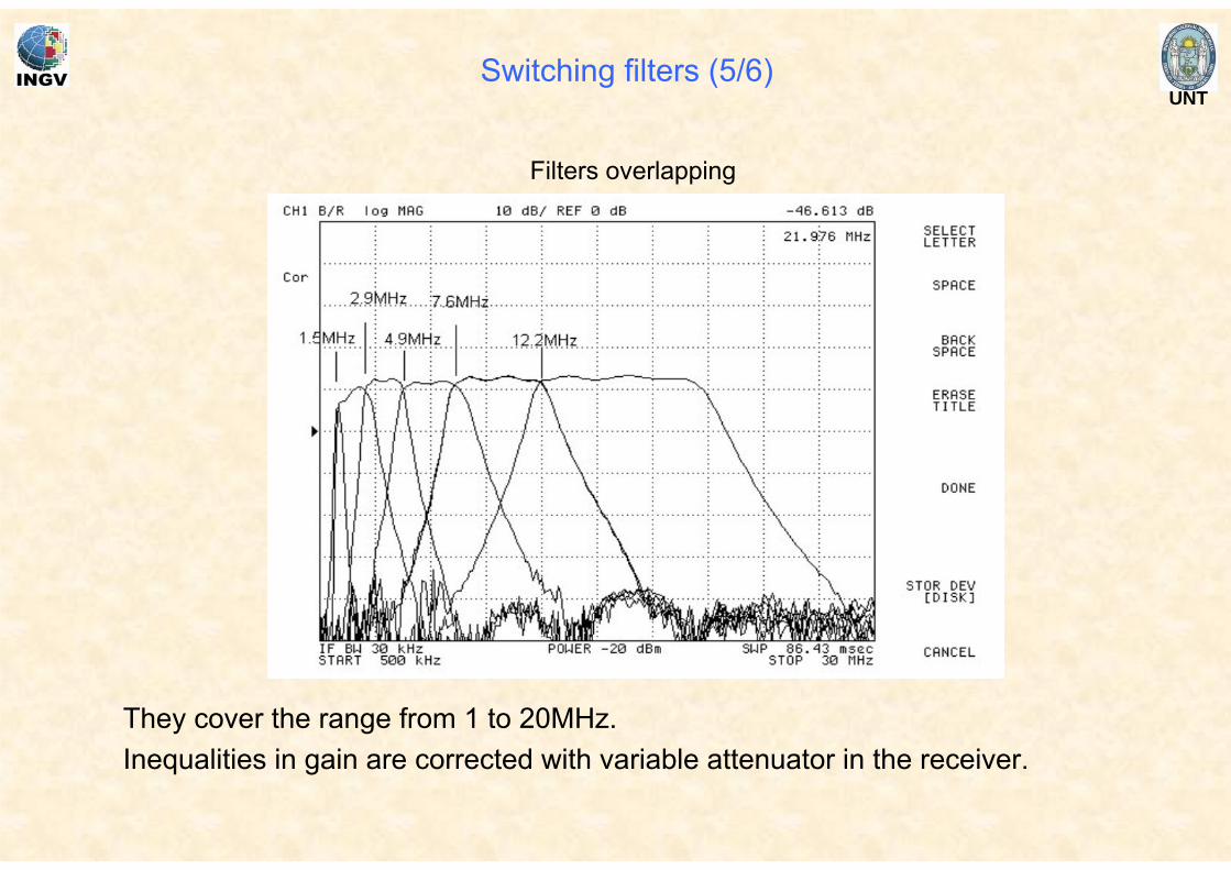
They cover the range from 1 to 20MHz.Inequalities in gain are corrected with variable attenuator in the receiver.
Filters overlapping
Switching filters (5/6)
UNT
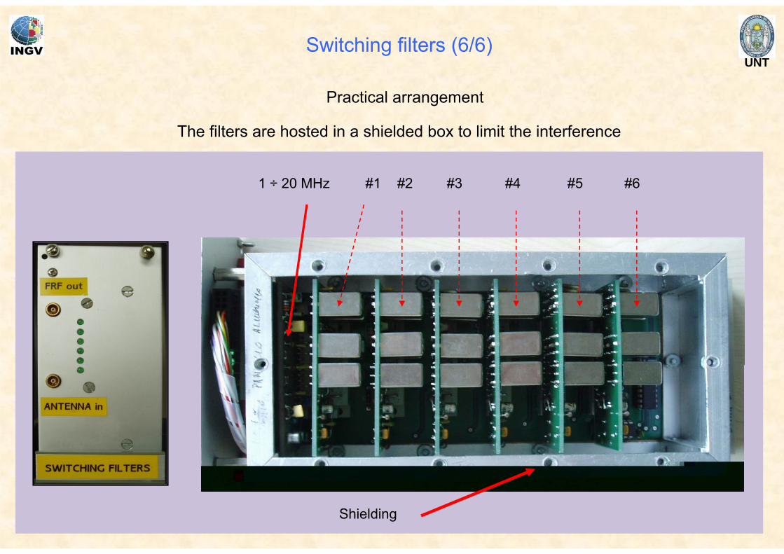
The filters are hosted in a shielded box to limit the interference
1 ÷ 20 MHz #1 #2 #3 #4 #5 #6
Shielding
Practical arrangement
Switching filters (6/6)
UNTReceiver (1/5)
UNT
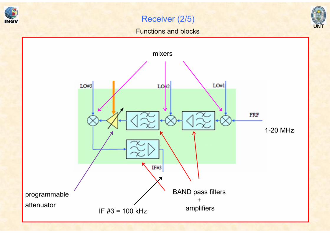
BAND pass filters +
amplifiers
mixers
programmableattenuator
1-20 MHz
IF #3 = 100 kHz
Functions and blocks
Receiver (2/5)
UNT
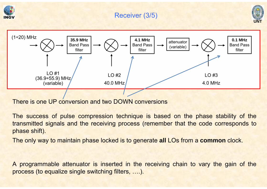
The success of pulse compression technique is based on the phase stability of the transmitted signals and the receiving process (remember that the code corresponds to phase shift).The only way to maintain phase locked is to generate all LOs from a common clock.
A programmable attenuator is inserted in the receiving chain to vary the gain of the process (to equalize single switching filters, ….).
(1÷20) MHz
LO #240.0 MHz
LO #34.0 MHz
35.9 MHzBand Pass
filter
4.1 MHzBand Pass
filter
0.1 MHzBand Pass
filter
LO #1(36.9÷55.9) MHz
(variable)
attenuator(variable)
There is one UP conversion and two DOWN conversions
Receiver (3/5)
UNT
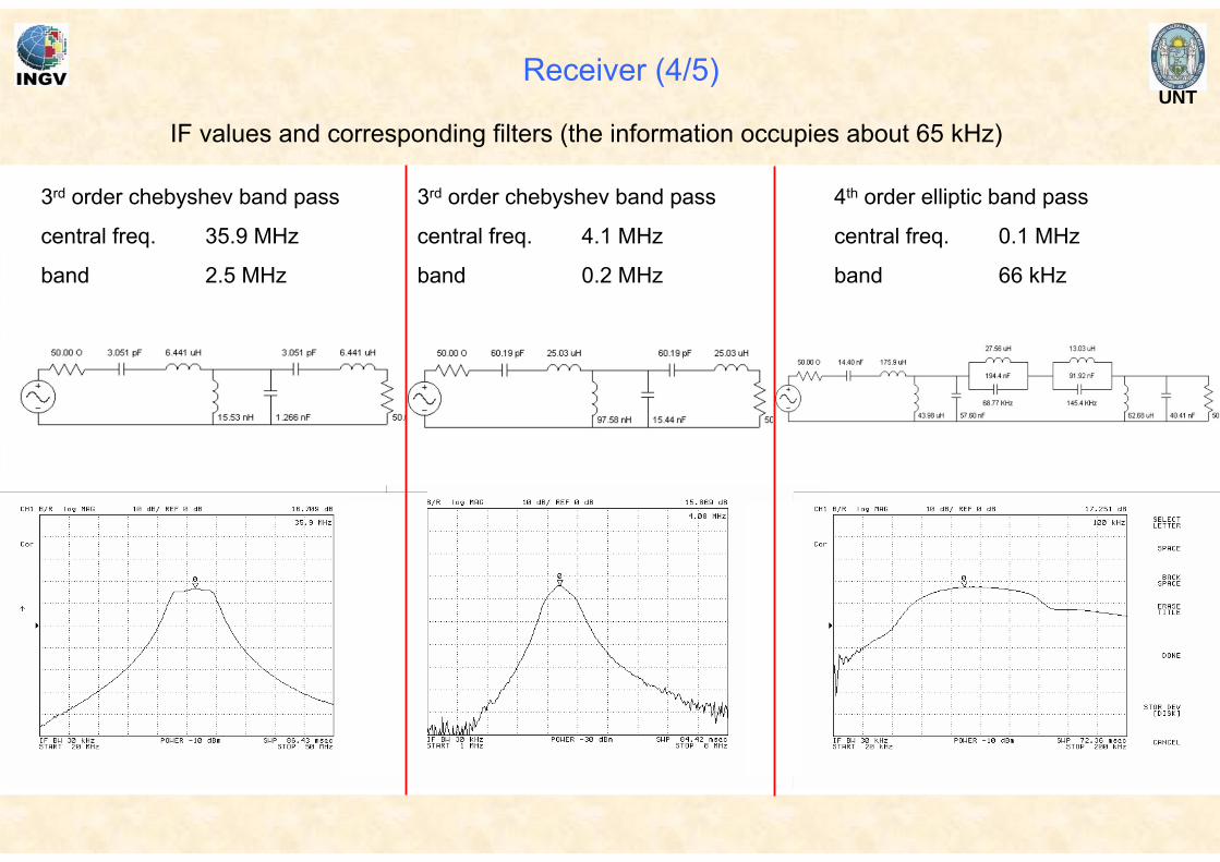
IF values and corresponding filters (the information occupies about 65 kHz)
3rd order chebyshev band pass
central freq. 35.9 MHz
band 2.5 MHz
3rd order chebyshev band pass
central freq. 4.1 MHz
band 0.2 MHz
4th order elliptic band pass
central freq. 0.1 MHz
band 66 kHz
Receiver (4/5)
UNT
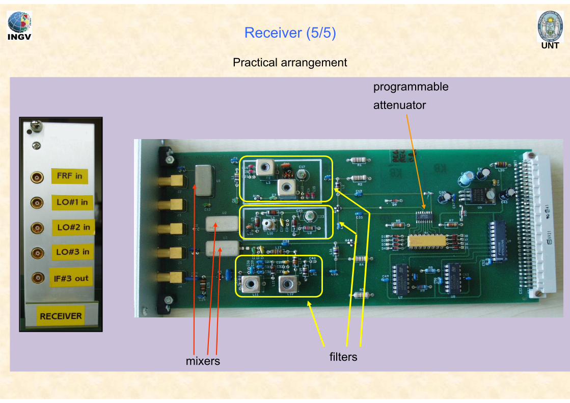
mixers
programmableattenuator
filters
Practical arrangement
Receiver (5/5)
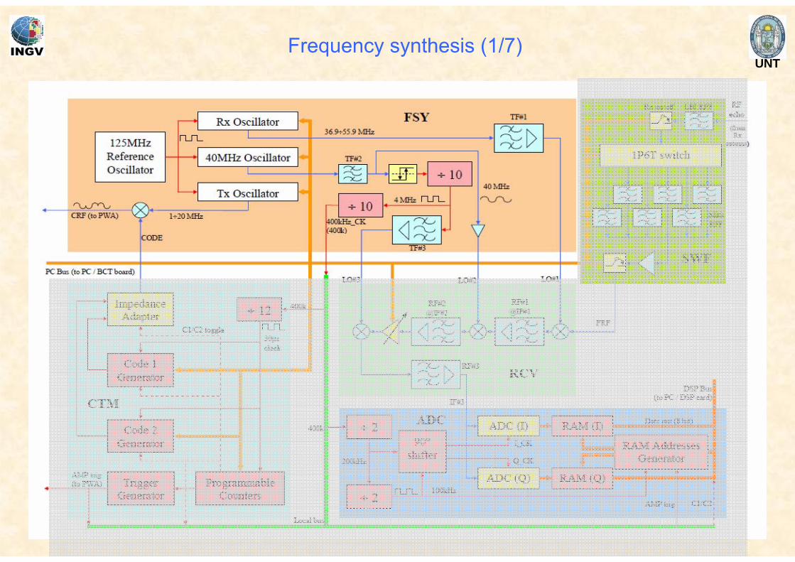
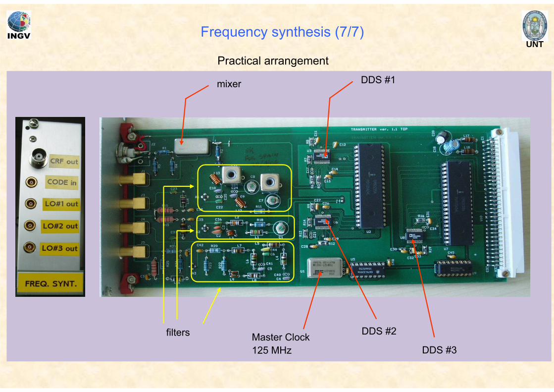
UNTFrequency synthesis (1/7)
UNT
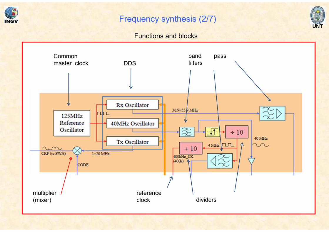
Functions and blocks
DDSCommonmaster clock
band pass filters
multiplier(mixer) dividers
reference clock
Frequency synthesis (2/7)
UNT
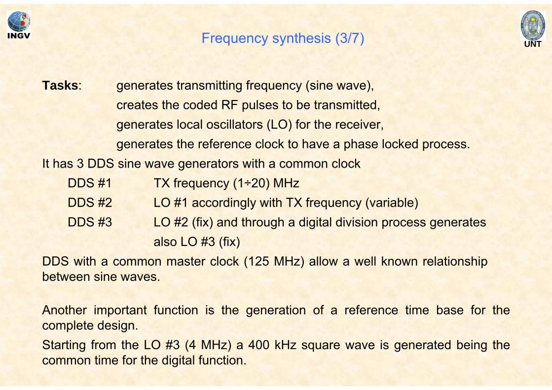
Tasks: generates transmitting frequency (sine wave),creates the coded RF pulses to be transmitted,generates local oscillators (LO) for the receiver,generates the reference clock to have a phase locked process.
It has 3 DDS sine wave generators with a common clockDDS #1 TX frequency (1÷20) MHzDDS #2 LO #1 accordingly with TX frequency (variable)DDS #3 LO #2 (fix) and through a digital division process generates
also LO #3 (fix)DDS with a common master clock (125 MHz) allow a well known relationship between sine waves.
Another important function is the generation of a reference time base for the complete design.Starting from the LO #3 (4 MHz) a 400 kHz square wave is generated being the common time for the digital function.
Frequency synthesis (3/7)
UNT
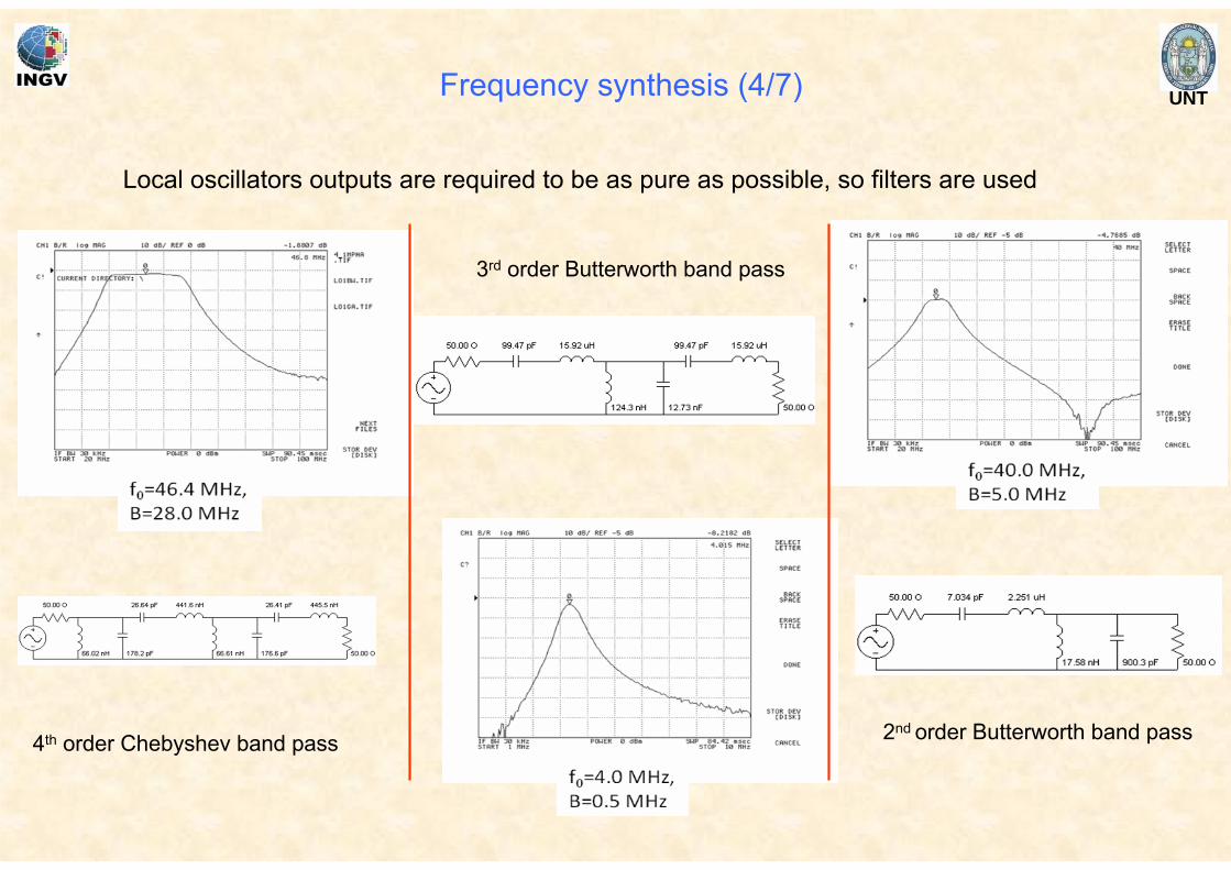
Local oscillators outputs are required to be as pure as possible, so filters are used
2nd order Butterworth band pass
3rd order Butterworth band pass
4th order Chebyshev band pass
Frequency synthesis (4/7)
UNT
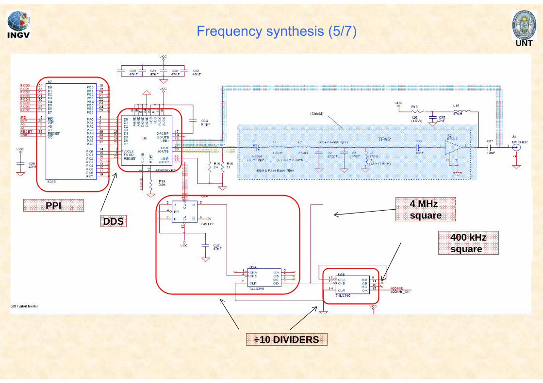
÷10 DIVIDERS
PPIDDS
4 MHzsquare
400 kHzsquare
Frequency synthesis (5/7)
UNT
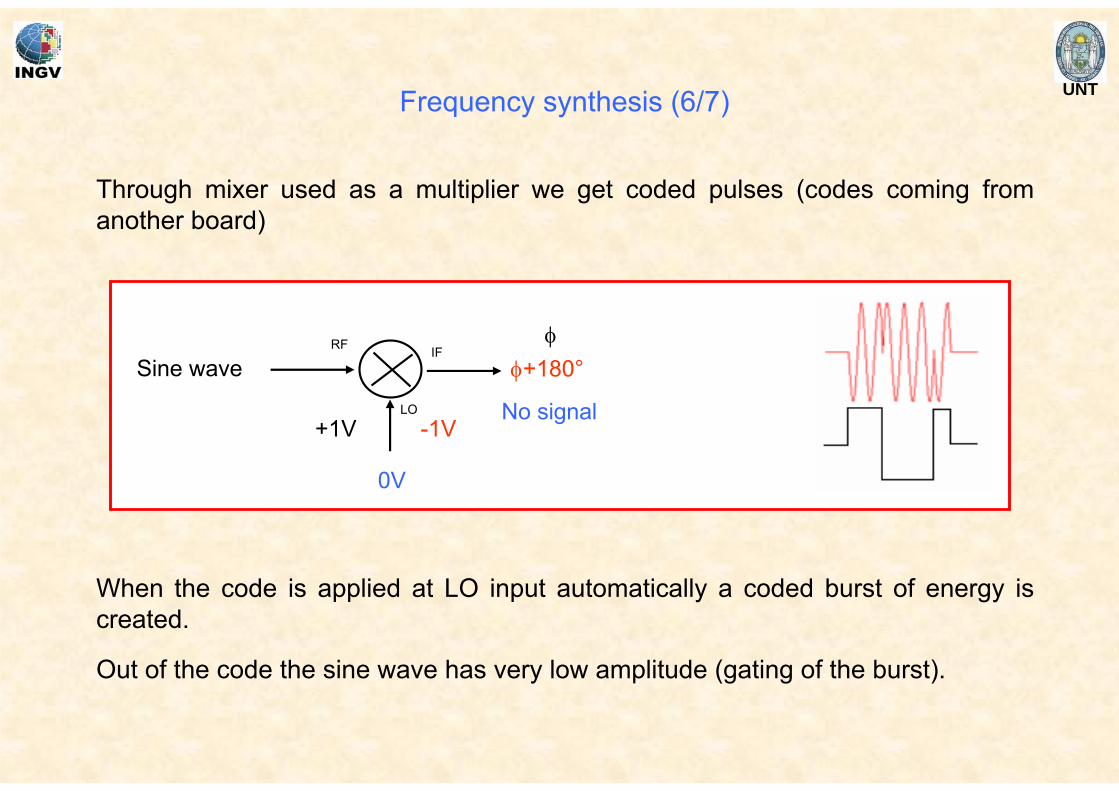
Through mixer used as a multiplier we get coded pulses (codes coming from another board)
When the code is applied at LO input automatically a coded burst of energy is created.
Out of the code the sine wave has very low amplitude (gating of the burst).
Sine wave
+1V -1V
φφ+180°
0V
No signalLO
IFRF
Frequency synthesis (6/7)
UNT
DDS #1
DDS #2
DDS #3
mixer
Master Clock125 MHz
filters
Practical arrangement
Frequency synthesis (7/7)
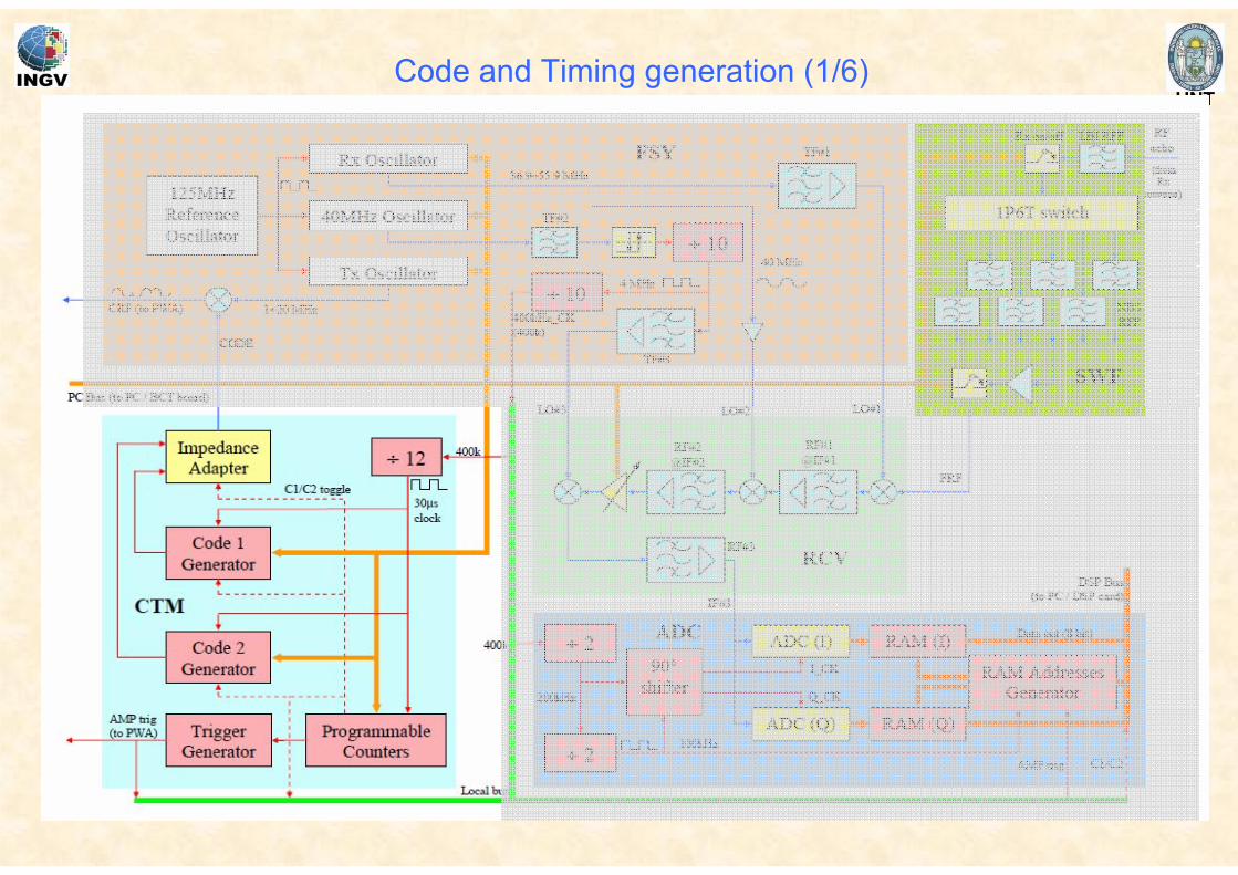
UNTCode and Timing generation (1/6)
UNT
Functions and blocks
reference clock
PC buscodes
generators+
50 ohm adapter
power amplifiertrigger
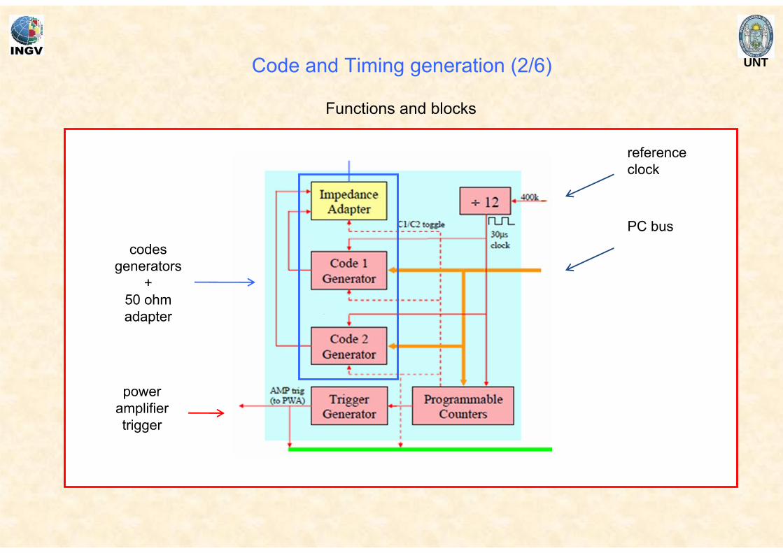
Code and Timing generation (2/6)
UNT
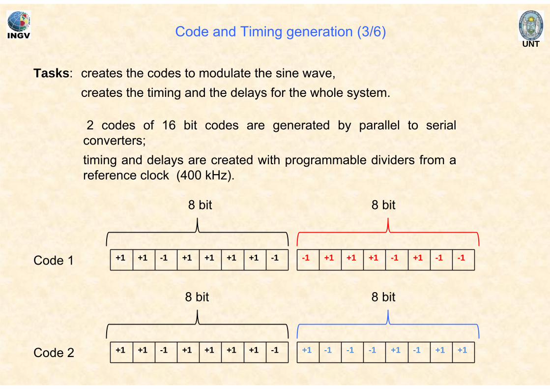
+1 +1 -1 +1 +1 +1 +1 -1
+1 +1 -1 +1 +1 +1 +1 -1
-1 +1 +1 +1 -1 +1 -1 -1
+1 -1 -1 -1 +1 -1 +1 +1
Tasks: creates the codes to modulate the sine wave,creates the timing and the delays for the whole system.
Code 1
8 bit 8 bit
Code 2
8 bit8 bit
2 codes of 16 bit codes are generated by parallel to serial converters;timing and delays are created with programmable dividers from a reference clock (400 kHz).
Code and Timing generation (3/6)
UNT
A common reference clock (2.5 μs ↔ 400 kHz) is the input for programmable
counters; so every generated time interval or delay is a multiple of the reference
clock period .
For instance the sub pulse time is 30 μs (2.5 μs x 12)
This guarantees that all signal in AIS are phase locked.
We can program: pulse repetition frequency, distance between the codes, the
codes themselves, number of bit representing the code and the pulse width.
Code and Timing generation (4/6)
UNT
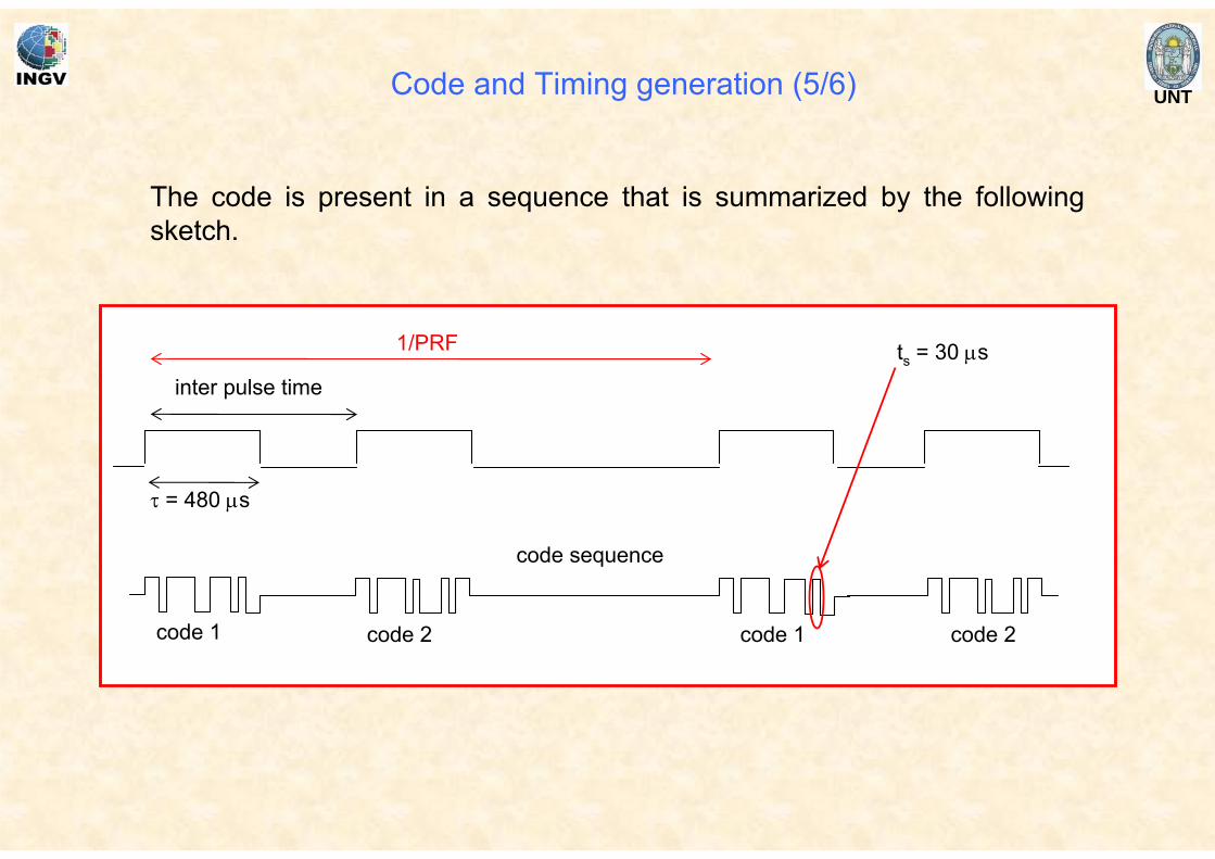
The code is present in a sequence that is summarized by the following sketch.
code sequence
code 1 code 1code 2 code 2
τ = 480 μs
1/PRF
inter pulse timets = 30 μs
Code and Timing generation (5/6)
UNT
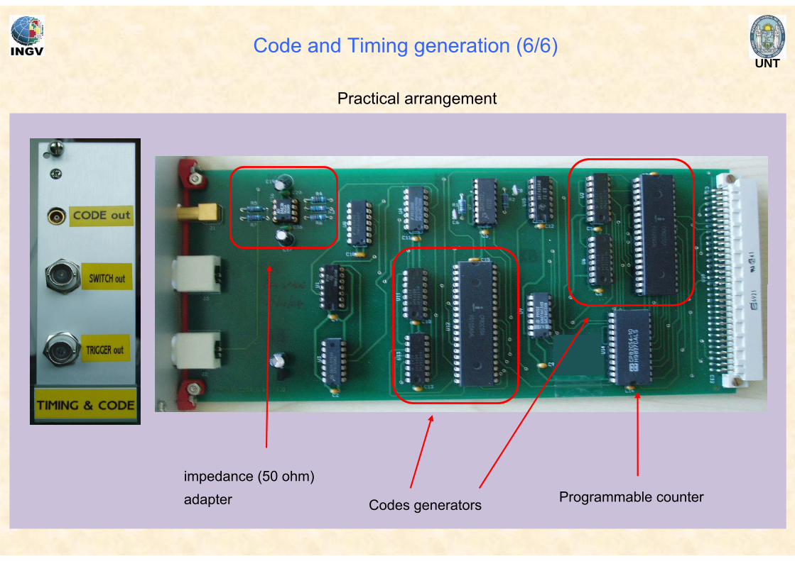
Programmable counterCodes generators
impedance (50 ohm)adapter
Practical arrangement
Code and Timing generation (6/6)
UNTAnalog To Digital conversion (1/5)
UNT
Functions and blocks
IF #3 (50 ohm)
8 bit ADC s local memories
sampling timing generator
address generator
Analog To Digital conversion (2/5)
UNT
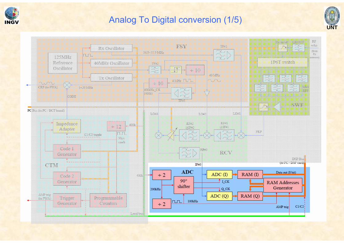
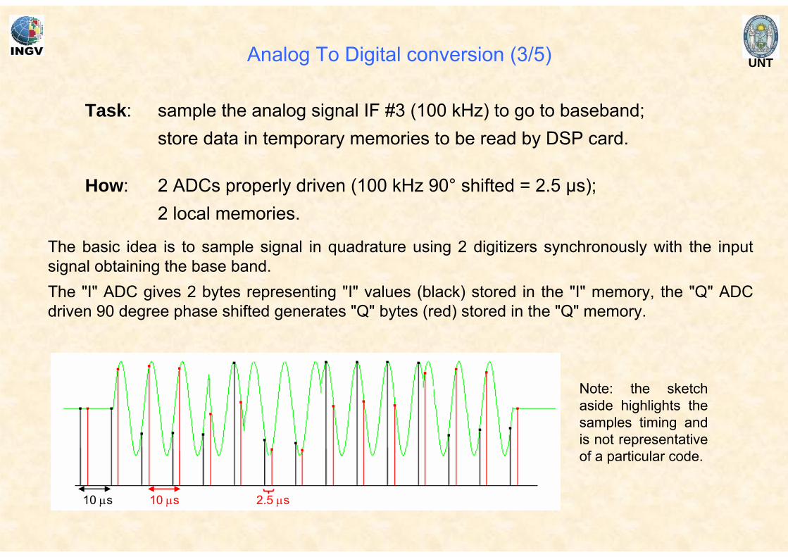
The basic idea is to sample signal in quadrature using 2 digitizers synchronously with the input signal obtaining the base band.The "I" ADC gives 2 bytes representing "I" values (black) stored in the "I" memory, the "Q" ADC driven 90 degree phase shifted generates "Q" bytes (red) stored in the "Q" memory.
Task: sample the analog signal IF #3 (100 kHz) to go to baseband;store data in temporary memories to be read by DSP card.
10 μs 10 μs 2.5 μs
How: 2 ADCs properly driven (100 kHz 90° shifted = 2.5 μs);2 local memories.
Analog To Digital conversion (3/5)
Note: the sketch aside highlights the samples timing and is not representative of a particular code.
UNT
After a pulse is emitted the listening time starts: during this time IF #3 (100 kHz)
is digitized at the the same frequency, getting the baseband.
During this time 512 Ik values and 512 Qk values are sampled and stored in two
local memories; consequently the listening time lasts 5.12 ms.
While samples are generated by ADCs memories are addressed synchronously.
After completion of this phase, the processing signal starts in DSP board.
Analog To Digital conversion (4/5)
UNT
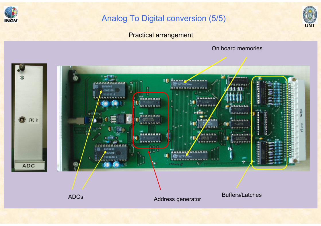
ADCs Address generator
On board memories
Buffers/Latches
Practical arrangement
Analog To Digital conversion (5/5)
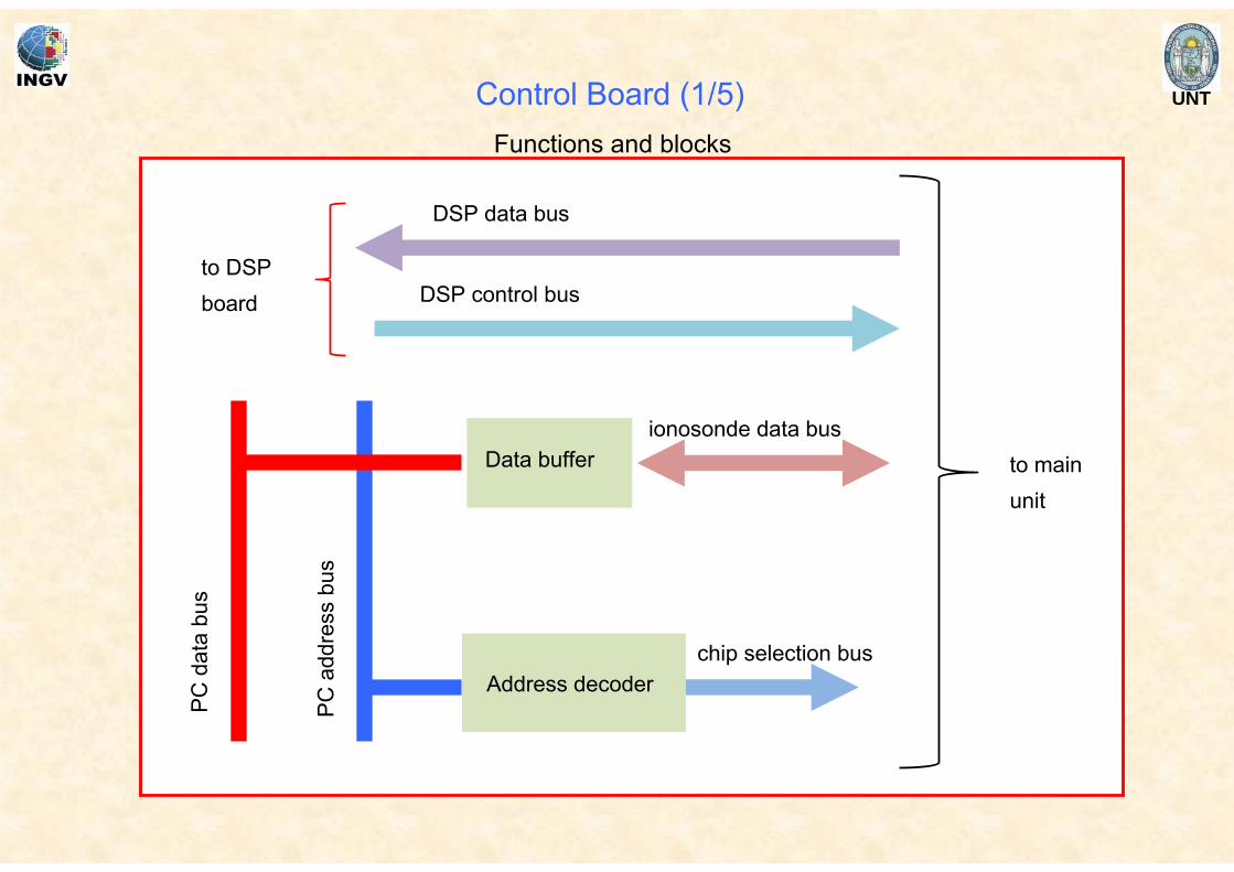
UNT
Functions and blocks
Data buffer
Address decoder
PC
dat
a bu
s
PC
add
ress
bus
DSP data bus
ionosonde data busto mainunit
chip selection bus
DSP control busto DSPboard
Control Board (1/5)
UNT
Task: to program ionosonde 's devices;
to join PC and DSP data busses (single cable communication);
to allow data bus of ionosonde communicating with PC data bus.
It is a card inserted in the PC ISA bus.
It corresponds to a group of addresses not conflicting with other peripherals.
Valid addresses are programmable.
Control Board (2/5)
UNT
CSA0
A1
8 bit DATA BUS
8255, 8254,registers ….
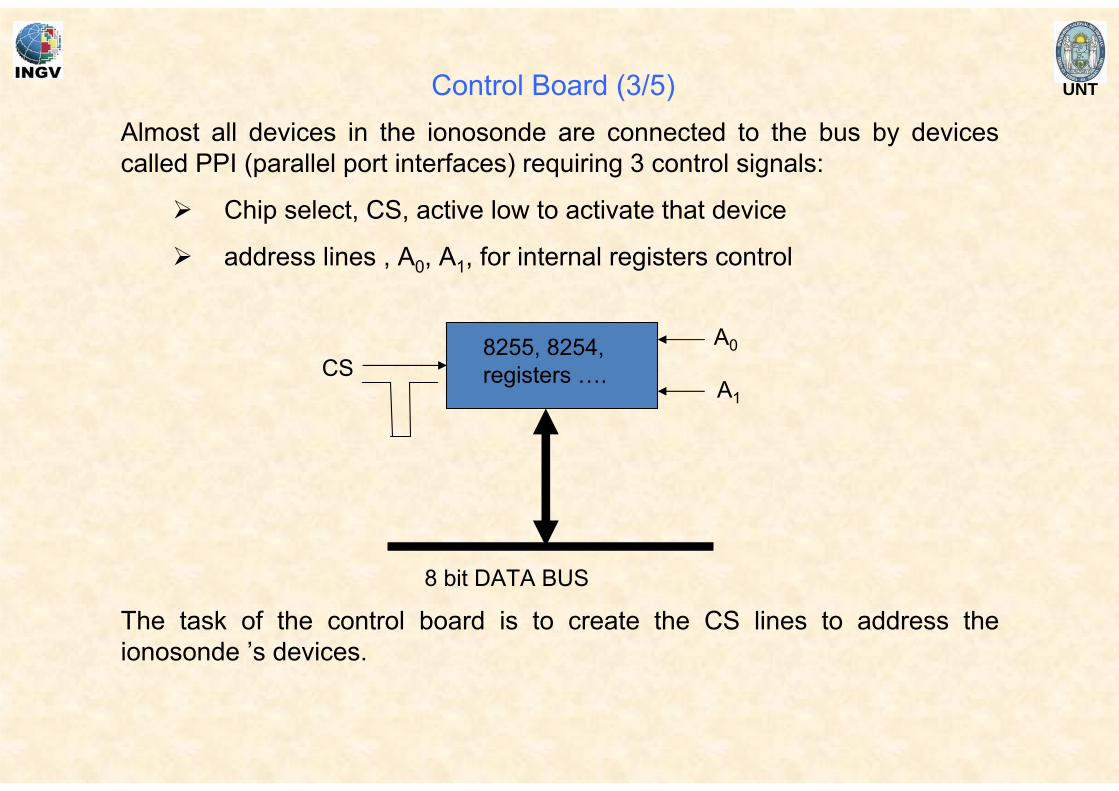
Almost all devices in the ionosonde are connected to the bus by devices called PPI (parallel port interfaces) requiring 3 control signals:
Chip select, CS, active low to activate that device
address lines , A0, A1, for internal registers control
The task of the control board is to create the CS lines to address the ionosonde ’s devices.
Control Board (3/5)
UNT
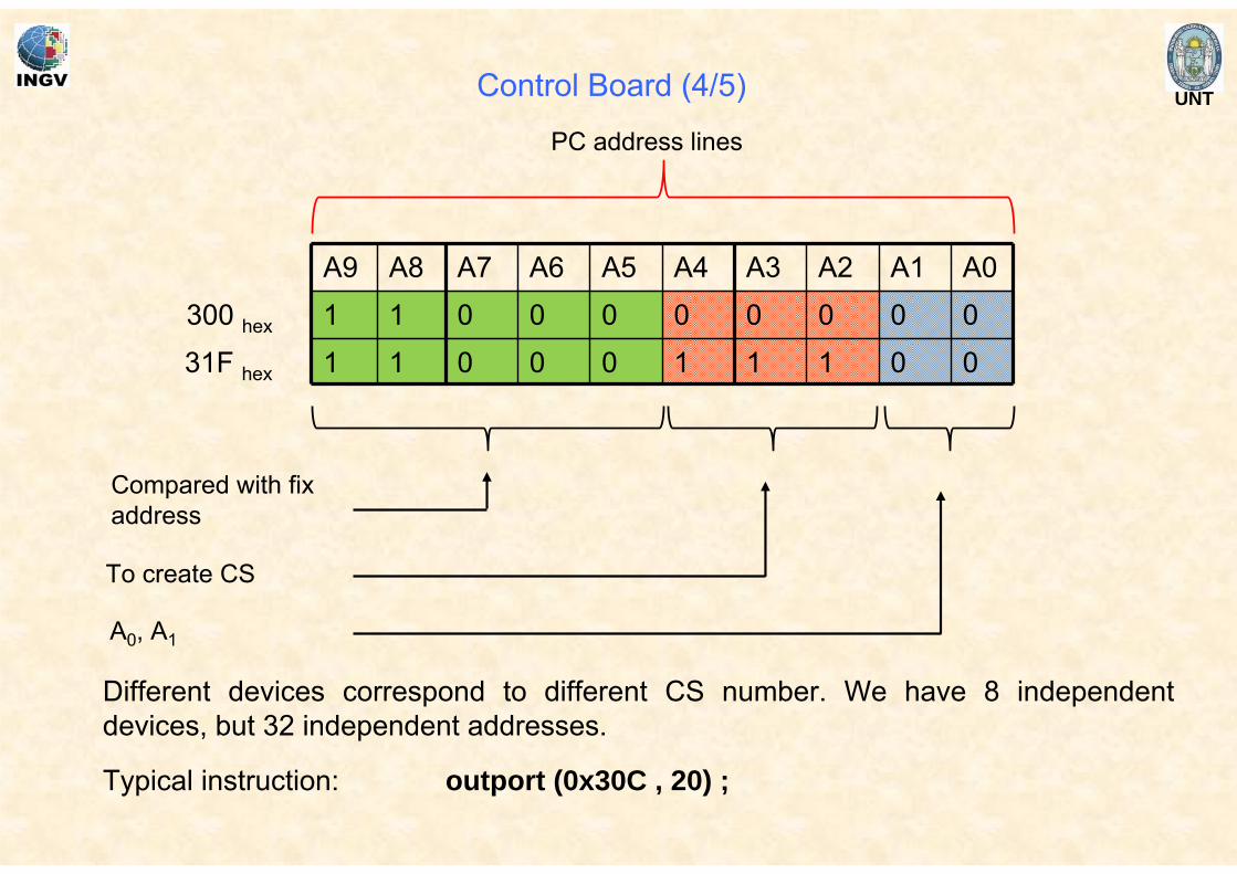
A9 A8 A7 A6 A5 A4 A3 A2 A1 A01 1 0 0 0 0 0 0 0 0
1 1 0 0 0 1 1 1 0 0
300 hex
31F hex
Compared with fixaddress
To create CS
A0, A1
Different devices correspond to different CS number. We have 8 independent devices, but 32 independent addresses.
Typical instruction: outport (0x30C , 20) ;
PC address lines
Control Board (4/5)
UNT
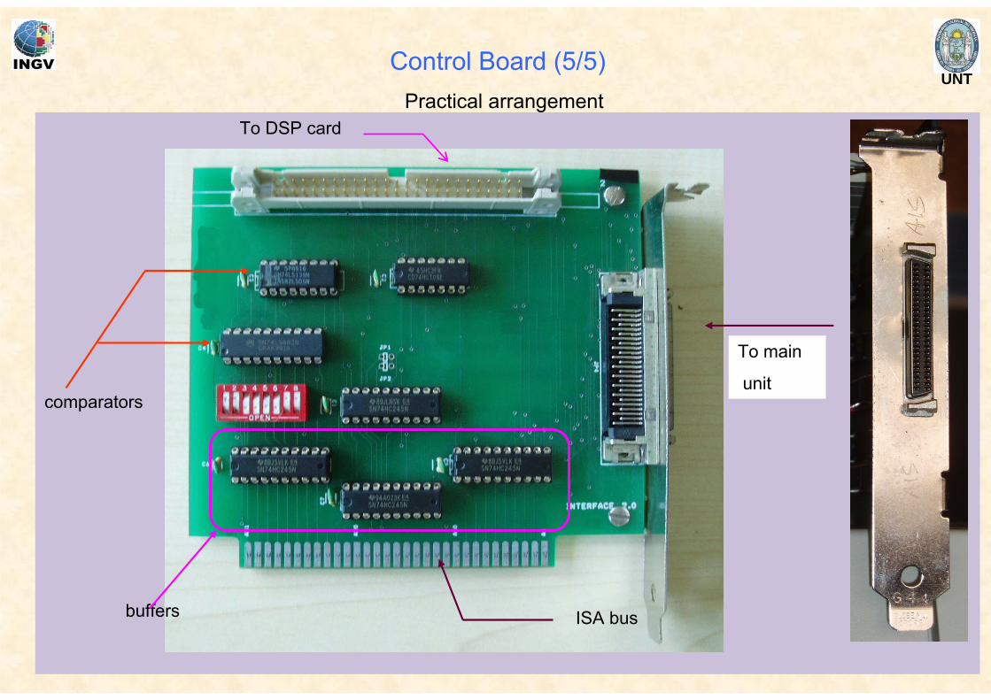
comparators
To DSP card
ISA bus
To main
unit
buffers
Practical arrangement
Control Board (5/5)
UNT
Task: to perform the analysis of the received echo to detect the codes and to find the height of the layer.
This task is accomplished with a program, running inside the board, loaded at the beginning of the sounding, that is independent of the main sounding software.
The complete process from echo to a dot on the screen goes through some steps:
• at the end of listening time, ADC card calls DSP that starts operation;
• DSP reads 512 samples (16 bit words), and start the analysis (code reconstruction, CFFT, filtering, correlation, integration, codes summation);
• when the programmed number of integration is reached DSP calls PC that will complete the analysis (CIFFT, threshold choice) creating the ionogram dot by dot.
DSP dialogues with ADC directly through a connection with interface board so to use one cable only.
DSP board (1/2)
UNT
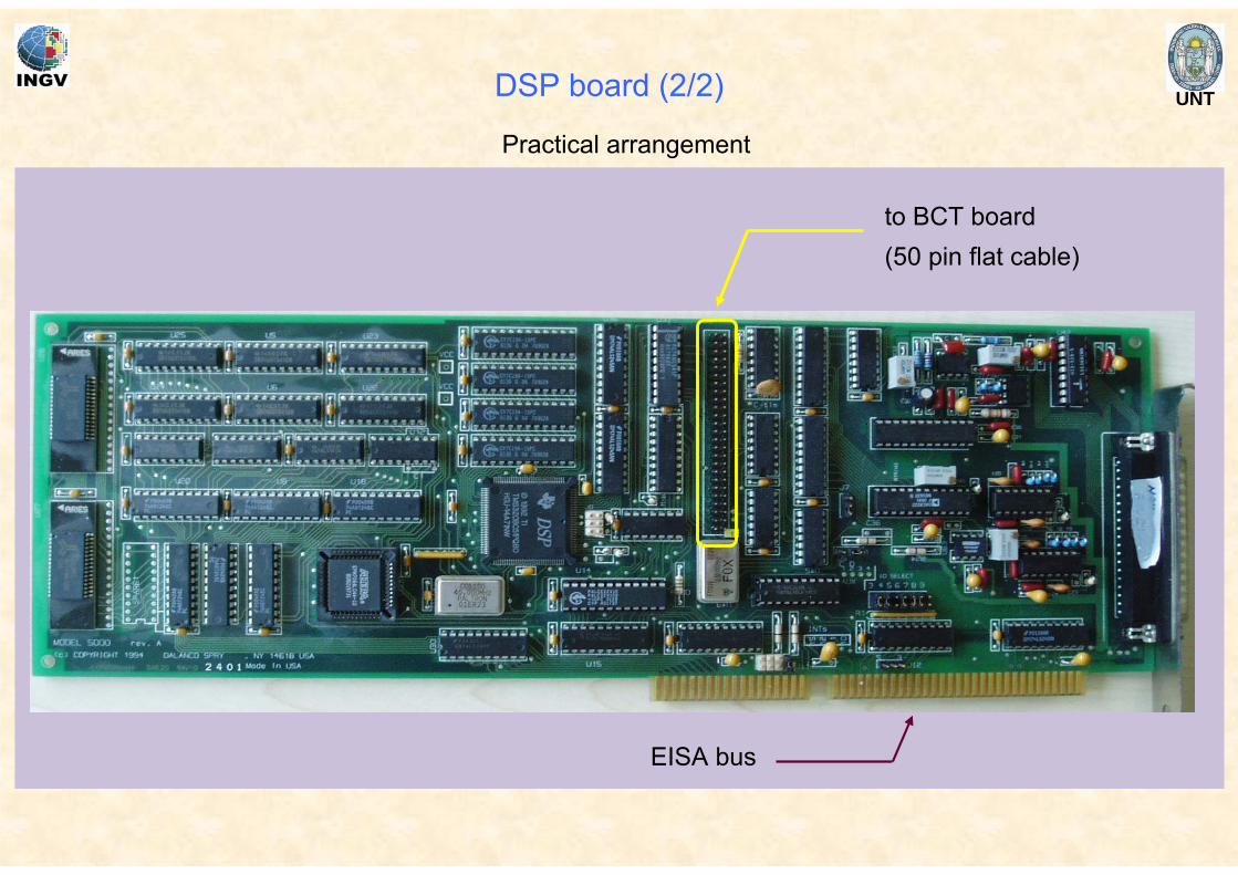
EISA bus
to BCT board(50 pin flat cable)
Practical arrangement
DSP board (2/2)
UNT
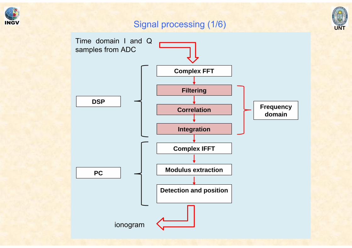
Time domain I and Q samples from ADC
Complex FFT
Filtering
Correlation
Integration
Complex IFFT
Modulus extraction
Frequency domain
Detection and position
DSP
PC
ionogram
Signal processing (1/6)
UNTSignal processing (2/6)
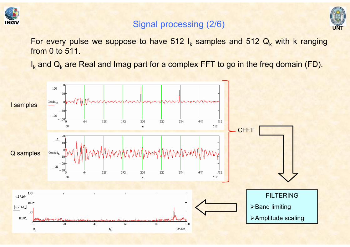
For every pulse we suppose to have 512 Ik samples and 512 Qk with k ranging from 0 to 511.Ik and Qk are Real and Imag part for a complex FFT to go in the freq domain (FD).
CFFT
I samples
Q samples
FILTERING
Band limiting
Amplitude scaling
UNT
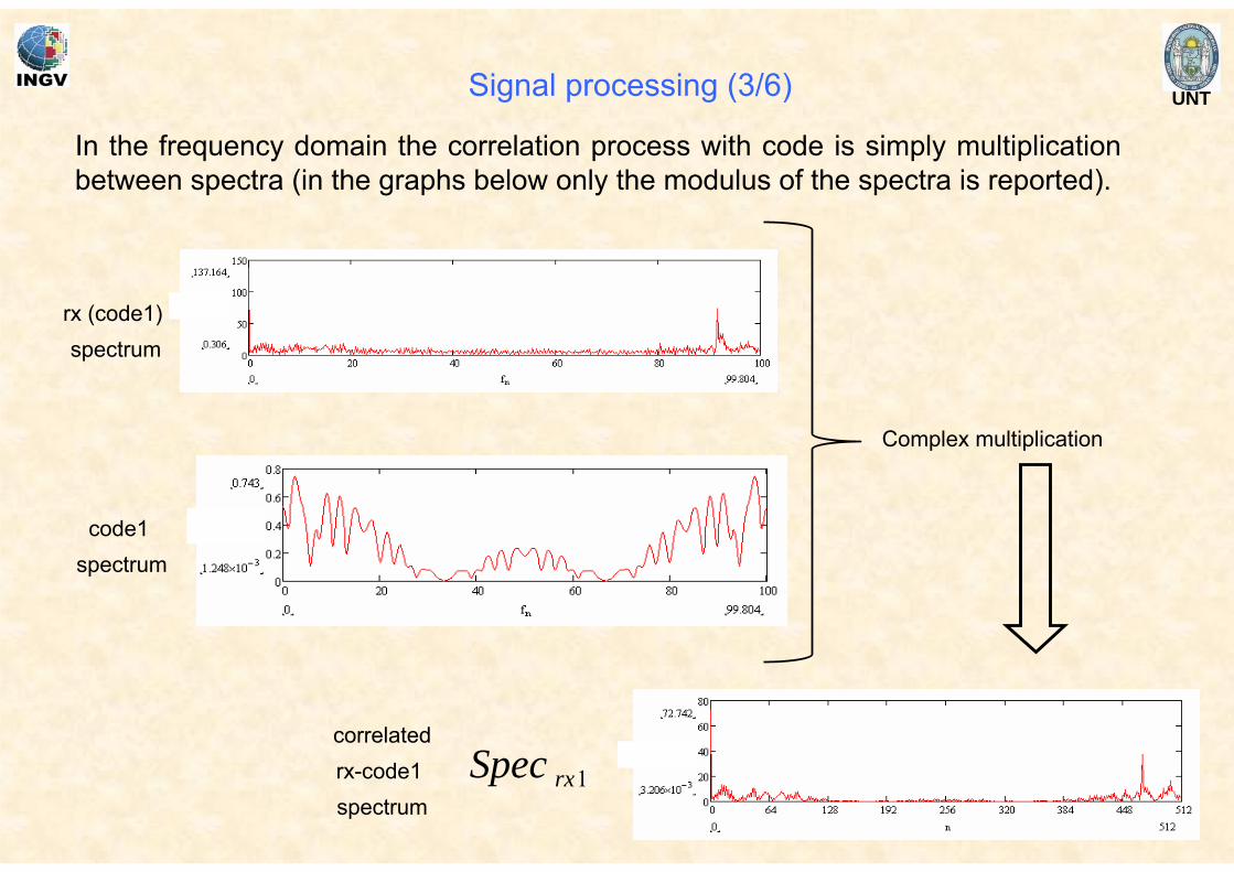
In the frequency domain the correlation process with code is simply multiplication between spectra (in the graphs below only the modulus of the spectra is reported).
Signal processing (3/6)
Complex multiplication
rx (code1) spectrum
code1 spectrum
correlatedrx-code1 spectrum
1rxSpec
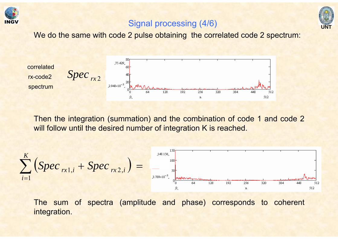
UNTWe do the same with code 2 pulse obtaining the correlated code 2 spectrum:
Then the integration (summation) and the combination of code 1 and code 2 will follow until the desired number of integration K is reached.
correlatedrx-code2 spectrum
2rxSpec
The sum of spectra (amplitude and phase) corresponds to coherentintegration.
Signal processing (4/6)
( ) =+∑=
K
iirxirx SpecSpec
1,2,1
UNT
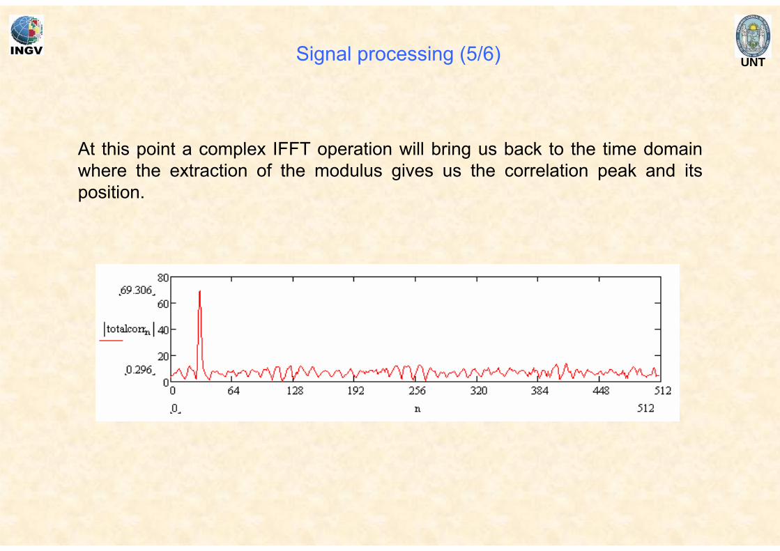
At this point a complex IFFT operation will bring us back to the time domain where the extraction of the modulus gives us the correlation peak and its position.
Signal processing (5/6)
UNT
In the following slides we will see some practical cases.
Signal processing (6/6)
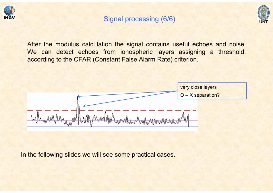
After the modulus calculation the signal contains useful echoes and noise. We can detect echoes from ionospheric layers assigning a threshold, according to the CFAR (Constant False Alarm Rate) criterion.
very close layersO – X separation?
UNT
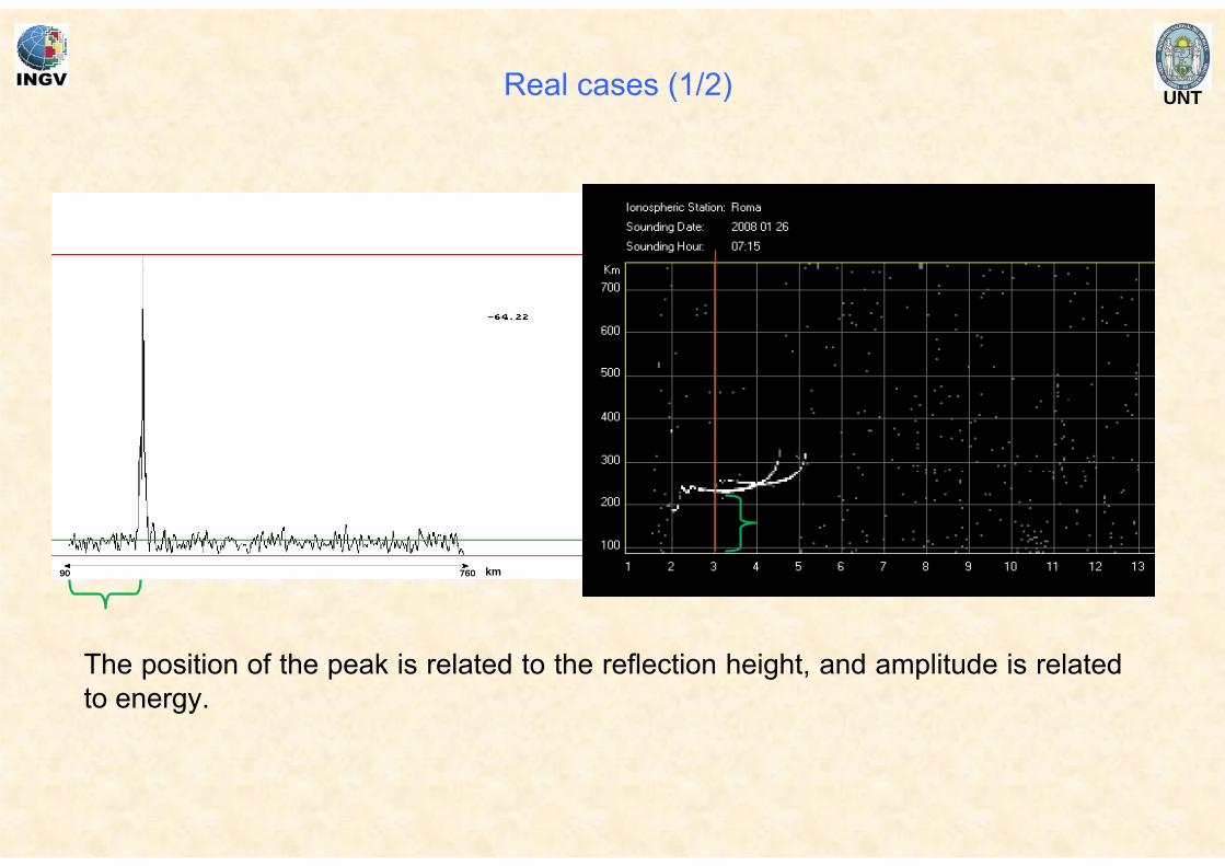
The position of the peak is related to the reflection height, and amplitude is related to energy.
Real cases (1/2)
km
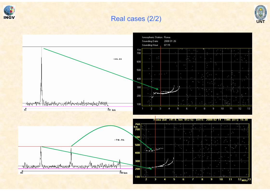
UNTReal cases (2/2)
km
km
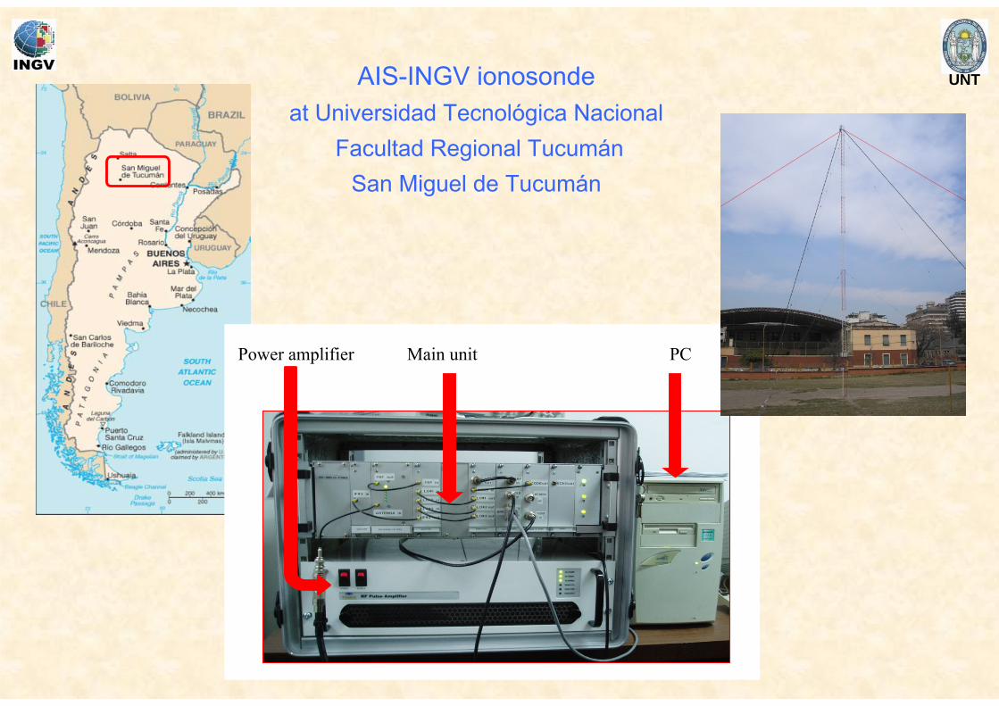
UNTAIS-INGV ionosonde at Universidad Tecnológica Nacional
Facultad Regional TucumánSan Miguel de Tucumán
Main unitPower amplifier PC
UNT
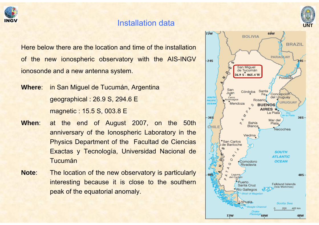
Where: in San Miguel de Tucumán, Argentina
geographical : 26.9 S, 294.6 E
magnetic : 15.5 S, 003.8 E
When: at the end of August 2007, on the 50th anniversary of the Ionospheric Laboratory in the Physics Department of the Facultad de CienciasExactas y Tecnología, Universidad Nacional de Tucumán
Note: The location of the new observatory is particularly interesting because it is close to the southern peak of the equatorial anomaly.
Installation data
Here below there are the location and time of the installation
of the new ionospheric observatory with the AIS-INGV
ionosonde and a new antenna system.
UNT
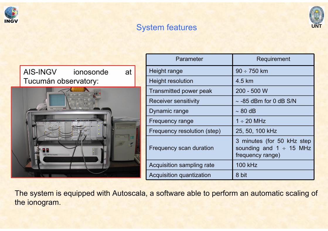
The system is equipped with Autoscala, a software able to perform an automatic scaling of the ionogram.
AIS-INGV ionosonde at Tucumán observatory:
Parameter Requirement
Height range 90 ÷ 750 km
Height resolution 4.5 km
Transmitted power peak 200 - 500 W
Receiver sensitivity ∼ -85 dBm for 0 dB S/N
Dynamic range ∼ 80 dB
Frequency range 1 ÷ 20 MHz
Frequency resolution (step) 25, 50, 100 kHz
Frequency scan duration3 minutes (for 50 kHz step sounding and 1 ÷ 15 MHz frequency range)
Acquisition sampling rate 100 kHz
Acquisition quantization 8 bit
System features
UNT
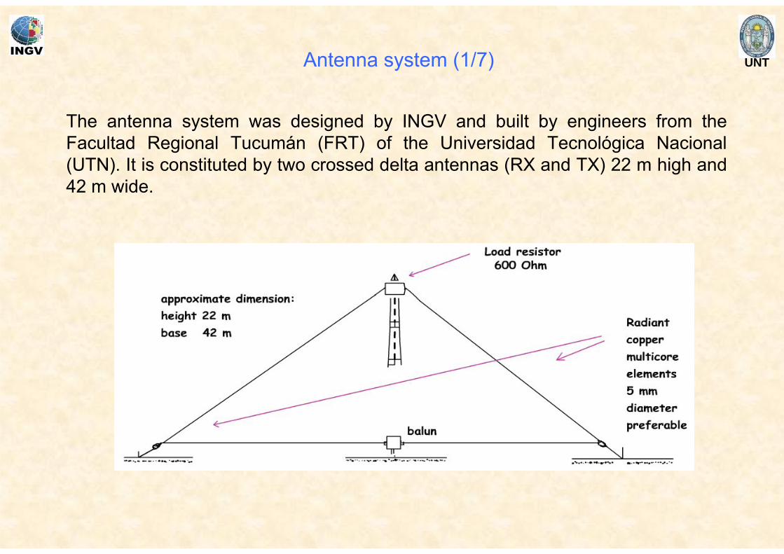
The antenna system was designed by INGV and built by engineers from the Facultad Regional Tucumán (FRT) of the Universidad Tecnológica Nacional(UTN). It is constituted by two crossed delta antennas (RX and TX) 22 m high and 42 m wide.
Antenna system (1/7)
UNT
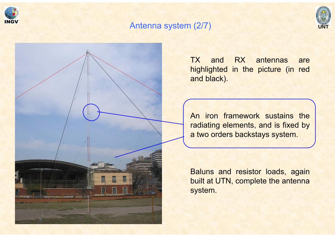
TX and RX antennas are highlighted in the picture (in red and black).
An iron framework sustains the radiating elements, and is fixed by a two orders backstays system.
Baluns and resistor loads, again built at UTN, complete the antenna system.
Antenna system (2/7)
UNT
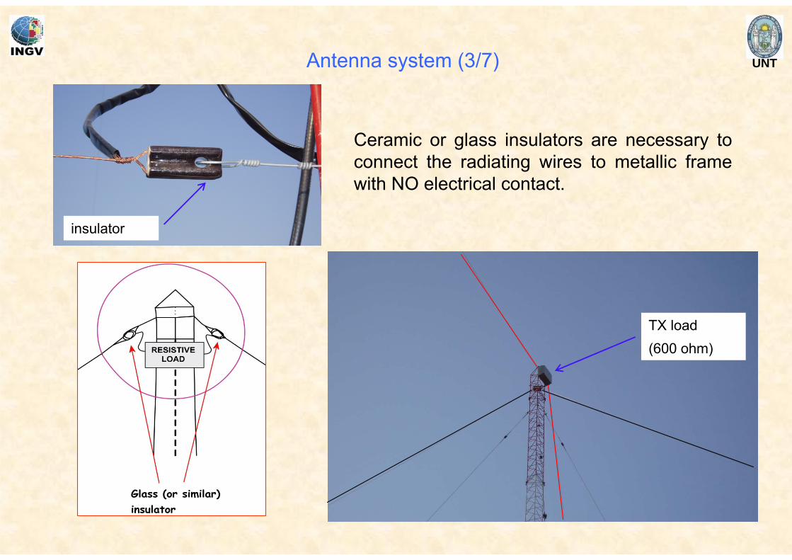
TX load(600 ohm)
insulator
Ceramic or glass insulators are necessary to connect the radiating wires to metallic frame with NO electrical contact.
Antenna system (3/7)
UNT
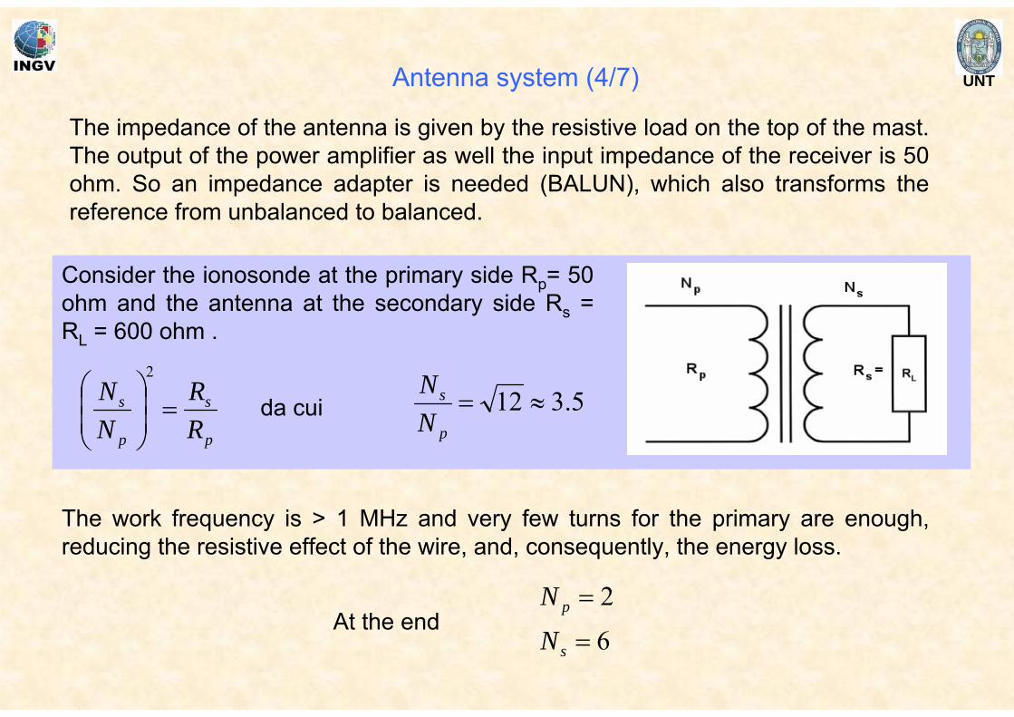
The impedance of the antenna is given by the resistive load on the top of the mast. The output of the power amplifier as well the input impedance of the receiver is 50 ohm. So an impedance adapter is needed (BALUN), which also transforms the reference from unbalanced to balanced.
p
s
p
s
RR
NN
=⎟⎟⎠
⎞⎜⎜⎝
⎛2
da cui 5.312 ≈=p
s
NN
The work frequency is > 1 MHz and very few turns for the primary are enough, reducing the resistive effect of the wire, and, consequently, the energy loss.
6
2
=
=
s
p
N
NAt the end
Consider the ionosonde at the primary side Rp= 50 ohm and the antenna at the secondary side Rs = RL = 600 ohm .
Antenna system (4/7)
UNT
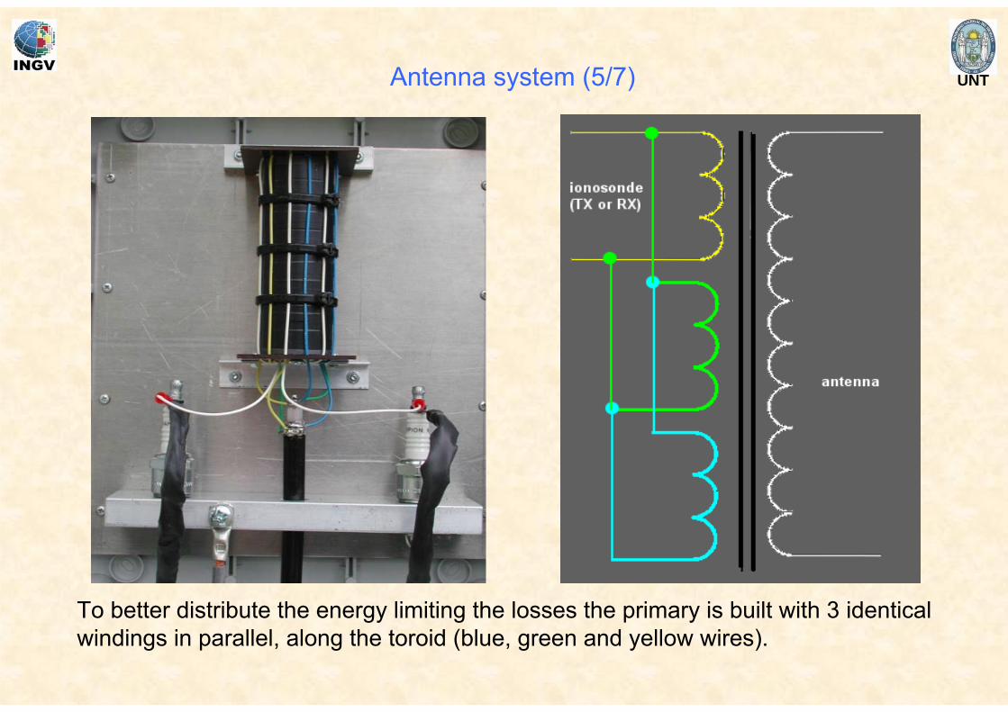
To better distribute the energy limiting the losses the primary is built with 3 identical windings in parallel, along the toroid (blue, green and yellow wires).
Antenna system (5/7)
UNT
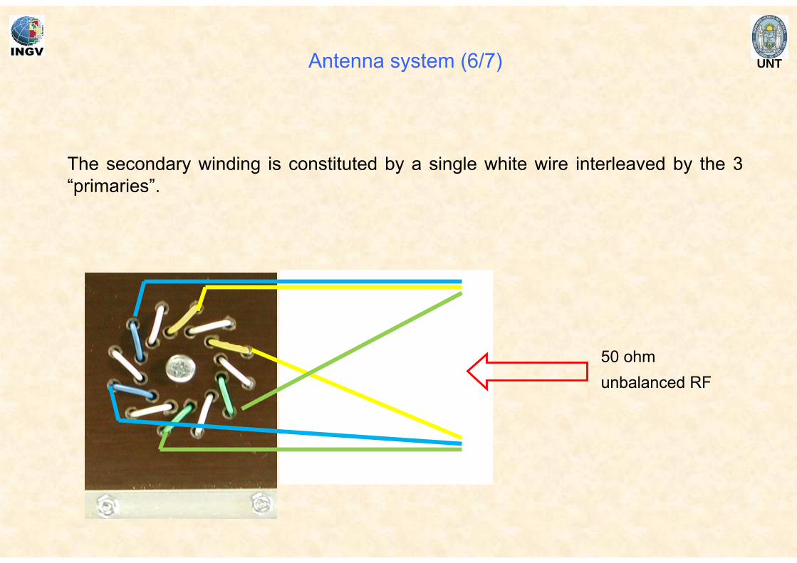
The secondary winding is constituted by a single white wire interleaved by the 3 “primaries”.
50 ohm unbalanced RF
Antenna system (6/7)
UNT
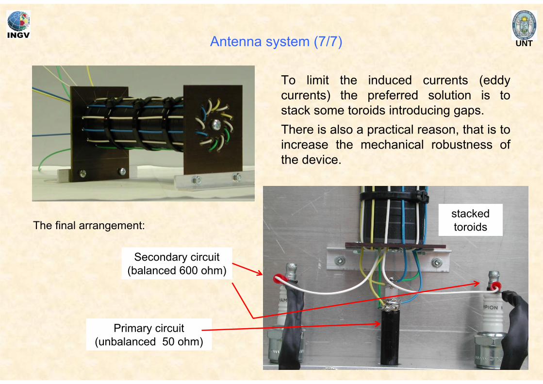
To limit the induced currents (eddy currents) the preferred solution is to stack some toroids introducing gaps.There is also a practical reason, that is to increase the mechanical robustness of the device.
The final arrangement:
Primary circuit (unbalanced 50 ohm)
Secondary circuit (balanced 600 ohm)
stacked toroids
Antenna system (7/7)
UNT
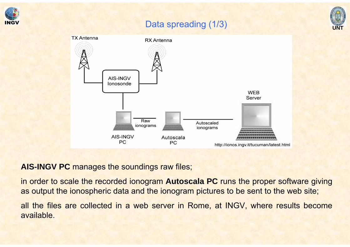
AIS-INGV PC manages the soundings raw files;
in order to scale the recorded ionogram Autoscala PC runs the proper software giving as output the ionospheric data and the ionogram pictures to be sent to the web site;
all the files are collected in a web server in Rome, at INGV, where results become available.
Data spreading (1/3)
UNT
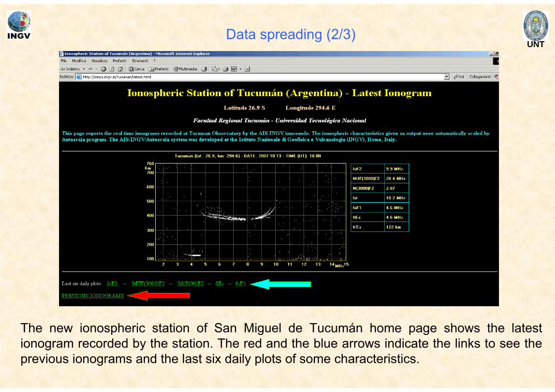
The new ionospheric station of San Miguel de Tucumán home page shows the latest ionogram recorded by the station. The red and the blue arrows indicate the links to see the previous ionograms and the last six daily plots of some characteristics.
Data spreading (2/3)
UNT
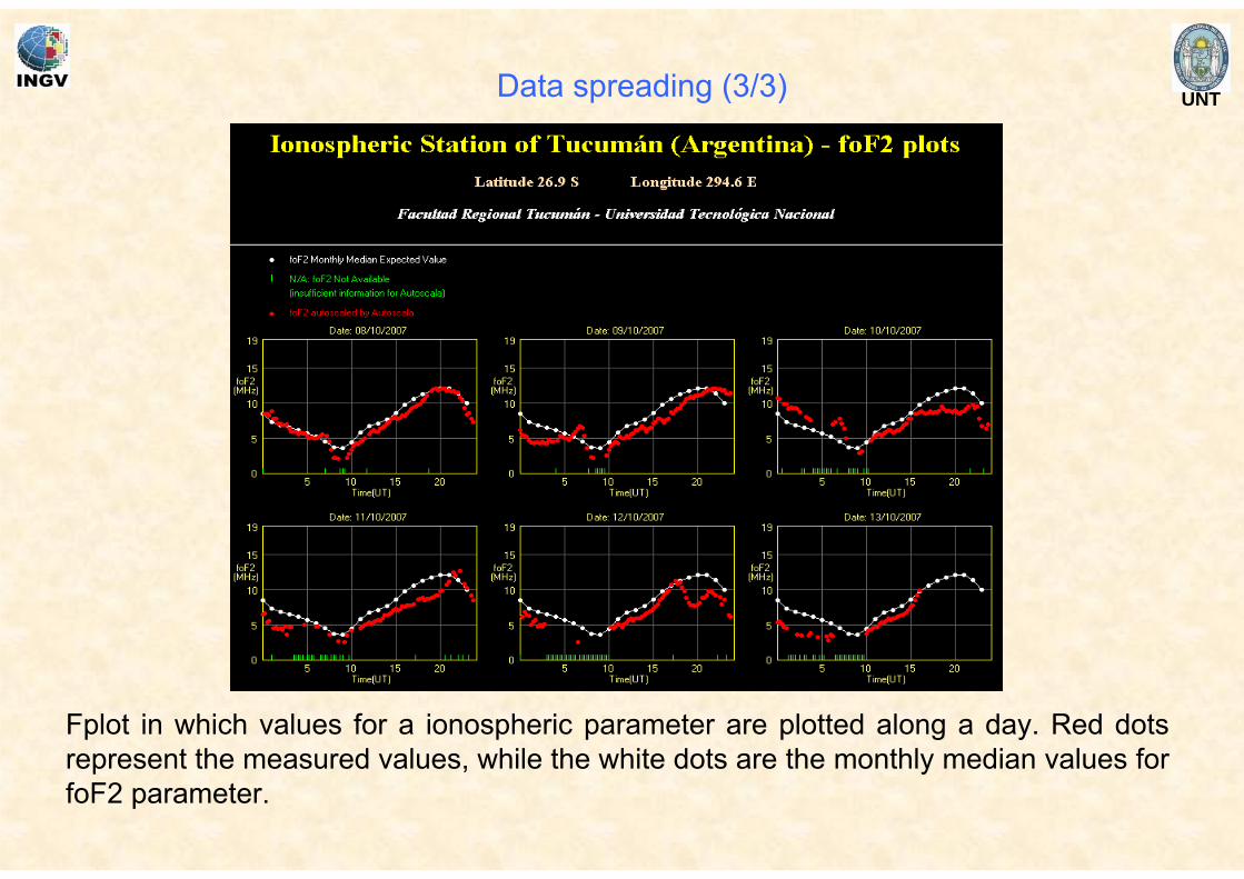
Fplot in which values for a ionospheric parameter are plotted along a day. Red dots represent the measured values, while the white dots are the monthly median values for foF2 parameter.
Data spreading (3/3)
UNT
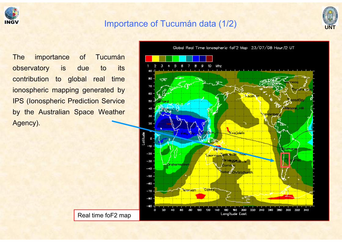
The importance of Tucumánobservatory is due to its contribution to global real time ionospheric mapping generated by IPS (Ionospheric Prediction Service by the Australian Space Weather Agency).
Importance of Tucumán data (1/2)
Real time foF2 map
UNTImportance of Tucumán data (2/2)
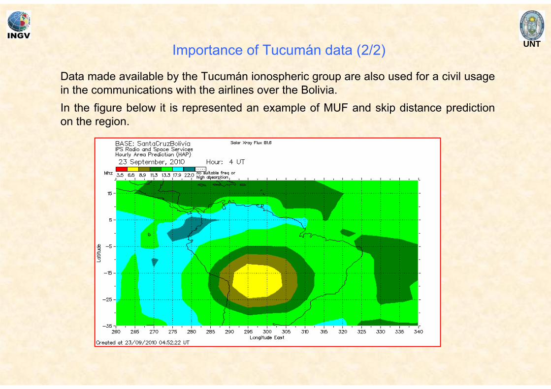
Data made available by the Tucumán ionospheric group are also used for a civil usage in the communications with the airlines over the Bolivia.In the figure below it is represented an example of MUF and skip distance prediction on the region.


![UWB Radars [EDocFind.com]](https://static.fdocuments.in/doc/165x107/577d2b9c1a28ab4e1eaae39f/uwb-radars-edocfindcom.jpg)