Traj-ARIMA: A Spatial-Time Series Model for Network ... · Traj-ARIMA: A Spatial-Time Series Model...
6
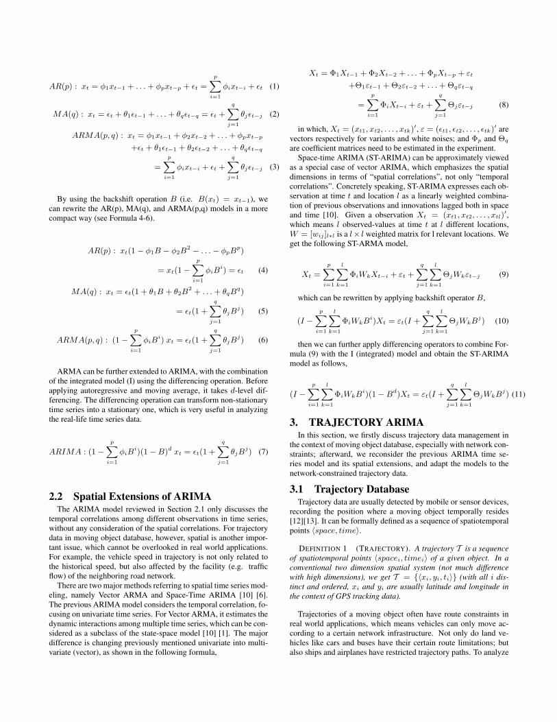
Traj-ARIMA: A Spatial-Time Series Model for Network-Constrained Trajectory Zhixian Yan EPFL - Ecole Polytechnique Fédérale de Lausanne, Switzerland zhixian.yan@epfl.ch ABSTRACT Trajectory data play an important role in analyzing real world appli- cations that involve movement features, e.g. natural and social phe- nomena such as bird migration, transportation management, urban planning and tourism analysis. Such trajectory data are a speical kind of time series with another focus on the spatial dimension be- sides the temporal one. Traditional time series models, especially the ARIMA (Auto-Regression Integrated Moving Average) model, have provided sound theoretical backgrounds and promoted many successful applications for managing and forecasting time-relevant sequential data. This paper aims at extending the ARIMA model with spatial dimension, and further applying it for the network- constrained trajectory data. We implement and evaluate the model for trajectory database, in the context of traffic application scenario about vehicle movement constrained under a given network infras- tructure. The proposed Traj-ARIMA model has many application perspectives, such as trajectory data regression and compression, outliers detection, traffic flow and vehicle speed prediction. In this paper, the major focus is on vehicle speed forecasting. Categories and Subject Descriptors H.2.8 [Database Management]: Database Applications—time se- ries database, spatial databases, GIS; G.3 [Probability and Statis- tics]: Time Series Analysis—Spatial-Time Series, Prediction General Terms Algorithm, Experimentation, Verification Keywords Trajectory Databases, Time Series Models, ARIMA, Computational Transportation Science (CTS) 1. INTRODUCTION With the advent of GPS and sensor-based tracking techniques, trajectory data become easily available and ubiquitous, both tech- nically and economically. The recorded trajectory includes a se- Permission to make digital or hard copies of all or part of this work for personal or classroom use is granted without fee provided that copies are not made or distributed for profit or commercial advantage and that copies bear this notice and the full citation on the first page. To copy otherwise, to republish, to post on servers or to redistribute to lists, requires prior specific permission and/or a fee. IWCTS’10, Nov 2, 2010 San Jose, CA, U.S.A. Copyright 2010 ACM 978-1-4503-0429-0/10/11... $10.00. quence of data points, and can be considered as a typical scenario of time series application. Time series analysis comprises statistical methods (e.g. autocorrelation and spectral analysis) that attempt to understand sequential data and do forecasting [1] [7]. With sound theoretical backgrounds and sustaining software packages, time se- ries have many successful applications in macroeconomics and fi- nances. However, for trajectory data in moving object database, time series method is still a fancy and trial topic need to be fur- ther exposited. Even with a couple of studies focusing on similar- ity search [4], mining periodic patterns [8], detecting outliers [9] in time series databases, there are less interconnections with pop- ular methods of time series analysis. In this paper, we study the conventional time series models, especially the time-domain driven analysis method ARIMA, and extend the model in the spatial di- mension to analyze and predict network-constrained trajectories in the context of moving object database. The rest of this paper is structured as follows: after a short intro- duction in Section 1, Section 2 reviews relevant conventional time series model, ARIMA in particular and its possible extensions for the spatial dimension, such as Vector-ARMA and ST-ARIMA; Sec- tion 3 addresses trajectories in a context of moving object database, and proposes the Traj-ARIMA model for network-constrained tra- jectories; the initial experimental results about vehicle speed analy- sis and prediction are presented in Section 4; and finally Section 5 points to conclusion and future work. 2. TIME SERIES MODEL AND SPATIAL EXTENSIONS In this section, we briefly study and review ARIMA (Autore- gressive Integrated Moving Average) model for time series, with the possible spatial extensions, such as the two major ones Vector ARMA and Space-Time ARIMA. 2.1 ARIMA Model As shown by Box and Jenkins [1], time series can be considered as stochastic processes from the statistical point of view. Time se- ries analysis provides models to represent the processes, in terms of many forms for modeling variations in the level of a process. Among those models, ARIMA (Autoregressive Integrated Moving Average) is a top-choice linear method. ARIMA combines the idea of the autoregressive (AR) model, the moving average (MA) model, and the integrated (I) model. Autoregressive process is regression on themselves, which means current value xt is a linear combina- tion of p (p is the order of AR) historical observations, plus a white noise t ; a moving average process of order q is a linear combina- tion of current noise and q historical noises; ARMA combines them, referring to the model with p autoregressive terms and q moving av- erage terms. The formulas of these three models are follows,
Transcript of Traj-ARIMA: A Spatial-Time Series Model for Network ... · Traj-ARIMA: A Spatial-Time Series Model...

Traj-ARIMA: A Spatial-Time Series Model forNetwork-Constrained Trajectory
Zhixian YanEPFL - Ecole Polytechnique Fédérale de Lausanne, Switzerland
ABSTRACTTrajectory data play an important role in analyzing real world appli-cations that involve movement features, e.g. natural and social phe-nomena such as bird migration, transportation management, urbanplanning and tourism analysis. Such trajectory data are a speicalkind of time series with another focus on the spatial dimension be-sides the temporal one. Traditional time series models, especiallythe ARIMA (Auto-Regression Integrated Moving Average) model,have provided sound theoretical backgrounds and promoted manysuccessful applications for managing and forecasting time-relevantsequential data. This paper aims at extending the ARIMA modelwith spatial dimension, and further applying it for the network-constrained trajectory data. We implement and evaluate the modelfor trajectory database, in the context of traffic application scenarioabout vehicle movement constrained under a given network infras-tructure. The proposed Traj-ARIMA model has many applicationperspectives, such as trajectory data regression and compression,outliers detection, traffic flow and vehicle speed prediction. In thispaper, the major focus is on vehicle speed forecasting.
Categories and Subject DescriptorsH.2.8 [Database Management]: Database Applications—time se-ries database, spatial databases, GIS; G.3 [Probability and Statis-tics]: Time Series Analysis—Spatial-Time Series, Prediction
General TermsAlgorithm, Experimentation, Verification
KeywordsTrajectory Databases, Time Series Models, ARIMA, ComputationalTransportation Science (CTS)
1. INTRODUCTIONWith the advent of GPS and sensor-based tracking techniques,
trajectory data become easily available and ubiquitous, both tech-nically and economically. The recorded trajectory includes a se-
Permission to make digital or hard copies of all or part of this work forpersonal or classroom use is granted without fee provided that copies arenot made or distributed for profit or commercial advantage and that copiesbear this notice and the full citation on the first page. To copy otherwise, torepublish, to post on servers or to redistribute to lists, requires prior specificpermission and/or a fee.IWCTS’10, Nov 2, 2010 San Jose, CA, U.S.A.Copyright 2010 ACM 978-1-4503-0429-0/10/11... $10.00.
quence of data points, and can be considered as a typical scenarioof time series application. Time series analysis comprises statisticalmethods (e.g. autocorrelation and spectral analysis) that attempt tounderstand sequential data and do forecasting [1] [7]. With soundtheoretical backgrounds and sustaining software packages, time se-ries have many successful applications in macroeconomics and fi-nances. However, for trajectory data in moving object database,time series method is still a fancy and trial topic need to be fur-ther exposited. Even with a couple of studies focusing on similar-ity search [4], mining periodic patterns [8], detecting outliers [9]in time series databases, there are less interconnections with pop-ular methods of time series analysis. In this paper, we study theconventional time series models, especially the time-domain drivenanalysis method ARIMA, and extend the model in the spatial di-mension to analyze and predict network-constrained trajectories inthe context of moving object database.
The rest of this paper is structured as follows: after a short intro-duction in Section 1, Section 2 reviews relevant conventional timeseries model, ARIMA in particular and its possible extensions forthe spatial dimension, such as Vector-ARMA and ST-ARIMA; Sec-tion 3 addresses trajectories in a context of moving object database,and proposes the Traj-ARIMA model for network-constrained tra-jectories; the initial experimental results about vehicle speed analy-sis and prediction are presented in Section 4; and finally Section 5points to conclusion and future work.
2. TIME SERIES MODEL AND SPATIALEXTENSIONS
In this section, we briefly study and review ARIMA (Autore-gressive Integrated Moving Average) model for time series, withthe possible spatial extensions, such as the two major ones VectorARMA and Space-Time ARIMA.
2.1 ARIMA ModelAs shown by Box and Jenkins [1], time series can be considered
as stochastic processes from the statistical point of view. Time se-ries analysis provides models to represent the processes, in termsof many forms for modeling variations in the level of a process.Among those models, ARIMA (Autoregressive Integrated MovingAverage) is a top-choice linear method. ARIMA combines the ideaof the autoregressive (AR) model, the moving average (MA) model,and the integrated (I) model. Autoregressive process is regressionon themselves, which means current value xt is a linear combina-tion of p (p is the order of AR) historical observations, plus a whitenoise εt; a moving average process of order q is a linear combina-tion of current noise and q historical noises; ARMA combines them,referring to the model with p autoregressive terms and q moving av-erage terms. The formulas of these three models are follows,
AR(p) : xt = φ1xt−1 + . . .+ φpxt−p + εt =
pXi=1
φixt−i + εt (1)
MA(q) : xt = εt + θ1εt−1 + . . .+ θqεt−q = εt +
qXj=1
θjεt−j (2)
ARMA(p, q) : xt = φ1xt−1 + φ2xt−2 + . . .+ φpxt−p
+εt + θ1εt−1 + θ2εt−2 + . . .+ θqεt−q
=
pXi=1
φixt−i + εt +
qXj=1
θjεt−j (3)
By using the backshift operation B (i.e. B(xt) = xt−1), wecan rewrite the AR(p), MA(q), and ARMA(p,q) models in a morecompact way (see Formula 4-6).
AR(p) : xt(1− φ1B − φ2B2 − . . .− φpBp)
= xt(1−pXi=1
φiBi) = εt (4)
MA(q) : xt = εt(1 + θ1B + θ2B2 + . . .+ θqB
q)
= εt(1 +
qXj=1
θjBj) (5)
ARMA(p, q) : (1−pXi=1
φiBi) xt = εt(1 +
qXj=1
θjBj) (6)
ARMA can be further extended to ARIMA, with the combinationof the integrated model (I) using the differencing operation. Beforeapplying autoregressive and moving average, it takes d-level dif-ferencing. The differencing operation can transform non-stationarytime series into a stationary one, which is very useful in analyzingthe real-life time series data.
ARIMA : (1−pXi=1
φiBi)(1−B)d xt = εt(1 +
qXj=1
θjBj) (7)
2.2 Spatial Extensions of ARIMAThe ARIMA model reviewed in Section 2.1 only discusses the
temporal correlations among different observations in time series,without any consideration of the spatial correlations. For trajectorydata in moving object database, however, spatial is another impor-tant issue, which cannot be overlooked in real world applications.For example, the vehicle speed in trajectory is not only related tothe historical speed, but also affected by the facility (e.g. trafficflow) of the neighboring road network.
There are two major methods referring to spatial time series mod-eling, namely Vector ARMA and Space-Time ARIMA [10] [6].The previous ARIMA model considers the temporal correlation, fo-cusing on univariate time series. For Vector ARMA, it estimates thedynamic interactions among multiple time series, which can be con-sidered as a subclass of the state-space model [10] [1]. The majordifference is changing previously mentioned univariate into multi-variate (vector), as shown in the following formula,
Xt = Φ1Xt−1 + Φ2Xt−2 + . . .+ ΦpXt−p + εt
+Θ1εt−1 + Θ2εt−2 + . . .+ Θqεt−q
=
pXi=1
ΦiXt−i + εt +
qXj=1
Θjεt−j (8)
in which, Xt = (xt1, xt2, . . . , xtk)′, ε = (εt1, εt2, . . . , εtk)′ arevectors respectively for variants and white noises; and Φp and Θq
are coefficient matrices need to be estimated in the experiment.Space-time ARIMA (ST-ARIMA) can be approximately viewed
as a special case of vector ARIMA, which emphasizes the spatialdimensions in terms of “spatial correlations”, not only “temporalcorrelations”. Concretely speaking, ST-ARIMA expresses each ob-servation at time t and location l as a linearly weighted combina-tion of previous observations and innovations lagged both in spaceand time [10]. Given a observation Xt = (xt1, xt2, . . . , xtl)
′,which means l observed-values at time t at l different locations,W = [wij ]l∗l is a l× l weighted matrix for l relevant locations. Weget the following ST-ARMA model,
Xt =
pXi=1
lXk=1
ΦiWkXt−i + εt +
qXj=1
lXk=1
ΘjWkεt−j (9)
which can be rewritten by applying backshift operator B,
(I −pXi=1
lXk=1
ΦiWkBi)Xt = εt(I +
qXj=1
lXk=1
ΘjWkBj) (10)
then we can further apply differencing operators to combine For-mula (9) with the I (integrated) model and obtain the ST-ARIMAmodel as follows,
(I −pXi=1
lXk=1
ΦiWkBi)(1−Bd)Xt = εt(I +
qXj=1
lXk=1
ΘjWkBj) (11)
3. TRAJECTORY ARIMAIn this section, we firstly discuss trajectory data management in
the context of moving object database, especially with network con-straints; afterward, we reconsider the previous ARIMA time se-ries model and its spatial extensions, and adapt the models to thenetwork-constrained trajectory data.
3.1 Trajectory DatabaseTrajectory data are usually detected by mobile or sensor devices,
recording the position where a moving object temporally resides[12][13]. It can be formally defined as a sequence of spatiotemporalpoints 〈space, time〉.
DEFINITION 1 (TRAJECTORY). A trajectory T is a sequenceof spatiotemporal points 〈spacei, timei〉 of a given object. In aconventional two dimension spatial system (not much differencewith high dimensions), we get T = {〈xi, yi, ti〉} (with all i dis-tinct and ordered, xi and yi are usually latitude and longitude inthe context of GPS tracking data).
Trajectories of a moving object often have route constraints inreal world applications, which means vehicles can only move ac-cording to a certain network infrastructure. Not only do land ve-hicles like cars and buses have their certain route limitations; butalso ships and airplanes have restricted trajectory paths. To analyze

trajectory data and do reasonable prediction, a comprehensible so-lution ought to consider the underlying network structure. Thosenetwork constraints for moving object trajectories can be defined asa network or a graph as follows,
DEFINITION 2 (NETWORK CONSTRAINTS). A network con-strain for trajectories is a directed graph G = (V, E), in which V isthe set of vertex {v1, v2, . . . , vn}, and E is a edge set for connectingvertex {e1, e2, . . . , em}. E can be represented as a n × n matrixof vertex, i.e. [eij ]n×n, in which eij can be 0, 1,∞ respectively fordirect-connection, self-connection and no-connection .
For a traffic road network, a road segment can be modeled as anode, and the connections among those road segments are edges.Figure 1 shows an example road network, and the following matrixis about the edge matrix connecting the road segments, where 0means self-connection and ∞ means no connection. We can usethe matrix for computing spatial lags from the spatial-time seriesviewpoint, which will be further discussed in Section 3.3.
Figure 1: A example road network
M =
0BBBBB@
r1 r2 r3 r4 r5 r6
r1 0 1 1 1 ∞ ∞r2 ∞ 0 ∞ ∞ ∞ ∞r3 ∞ ∞ 0 ∞ ∞ ∞r4 ∞ 1 1 0 1 1r5 ∞ ∞ ∞ ∞ 0 ∞r6 ∞ ∞ ∞ 1 1 0
1CCCCCAReal world trajectories should be consistent with the underlying
network infrastructure, as an example shown in Fig. 2 (generated by[3]), which projects the trajectories of many moving object into theconsistent network. Therefore, trajectories from Definition 1 needto be refined with network constraints. The original GPS trackedlocation (xi, yi) in a trajectory T need to be map-matched intoroad segments in a certain road network. With the underlying net-work, trajectory data analysis can consider the spatial correlationsbetween the neighboring road segments.
DEFINITION 3 (NETWORK CONSTRAINED TRAJECTORY). Atrajectory under network constraints can be defined asT N = {T S,G}, where T S is a set of trajectories, which might be-long to one moving object or many different moving objects T S ={T1, T2, . . . , Tm}; G is the constrained network G = (V, E).
For each trajectory Tk, it is a sequence of GPS tracking data Tk ={〈xki, yki, tki〉}, as shown in Definition 1. By integrating networkconstraints and moving object information, the trajectory can berefined as Tk = {〈xki, yki, tki,mo_id, road_id〉}, where mo_idmeans ID of the moving object, road_id means the road networksegments that the spatial location 〈xki, yki〉 can be matched.
3.2 Time Series for TrajectoriesBefore proposing a fully supporting spatial-time series model for
trajectory database, we firstly just focus on the temporal correla-tions of sequential trajectory data. The main task is to transform the
Figure 2: Network constrained trajectories
initial GPS tracking trajectory data 〈xt, yt, ti〉 into a concrete timeseries. For trajectory data about moving object, one of the majorsequential issues is about velocity analysis. With the availabilityof speed model for moving object, we can do further queries aboutspeed forecasting and location prediction.
As GPS data are usually tracked very frequently in a short timeinterval (in our experiment case, tracking one record per second),we can approximately calculate the instant speed as the averagespeed between the previous node and the subsequent node as inFormula (12)1,
si =‖〈xi+1, yi+1〉 − 〈xi−1, yi−1〉‖22
ti+1 − ti−1(12)
Afterward, we can get the following trajectory speed time series(for each moving object):
〈s1, t1〉, 〈s2, t2〉, . . . , 〈sn, tn〉
Instead of analyzing the temporal correlations of trajectory in-stant speed at different time observations, we can also construct an-other time series model about distances, {〈d1, t1〉, 〈d2, d2〉, . . . , 〈dn, tn〉}where di = di−1 + ‖〈xi, yi〉 − 〈xi−1, yi−1〉‖22 and d0 = 0. In thispaper, we focus on using ARIMA and the extended spatial time se-ries model for trajectory speed time series analysis. We can easilyadapt univariate ARIMA model from Section 2.1 to construct thefollowing ARIMA model:
(1−pXi=1
φiBi) st = εt(1 +
qXj=1
θjBj) (13)
We follow Box-Jenkins’ typical steps to identify, estimate anddiagnose an ARIMA Model for vehicle speed time series: plot thedata and analyze the correlogram for variables; estimate parametersand fit the model; make diagnose checking and speed forecasting(mainly short-term forecasting). The experimental details will bepresented later.
3.3 Spatial-Time Series for TrajectoriesThe previous ARIMA model for trajectory speed analysis only
considers temporal dimension correlations, which means we modeland forecast trajectory speed only based on its historical speeds,1In some data sets, if the instant speed is captured by GPS devices,we can use is directly.
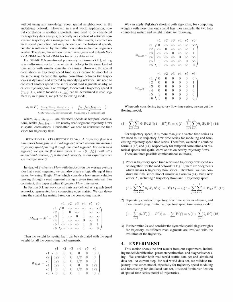
without using any knowledge about spatial neighborhood in theunderlying network. However, in a real world application, spa-tial correlation is another important issue need to be consideredfor trajectory data analysis, especially in a context of network con-strained trajectory data management. In other words, a correct ve-hicle speed prediction not only depends on the historical speeds,but also is influenced by the traffic flow status in the road segmentsnearby. Therefore, this section further investigates and extends Vec-tor ARIMA and ST-ARIMA for trajectory data series.
For ST-ARIMA mentioned previously in Formula (11), all xtiin a multivariate vector time series Xt belong to the same kind oftime series with similar semantic meanings. However, the spatialcorrelations in trajectory speed time series cannot be modeled inthe same way, because the spatial correlation between two trajec-tories is dynamic and affected by underlying network. We need toconstruct another speed time series about road segments nearby, socalled trajectory flow. For example, to forecast a trajectory speed at〈xi, yi, ti〉, where location 〈xi, yi〉 can be determined at road seg-ment r5 in Figure 1, we get the following model,
st = F ( st−1, st−2, st−3, . . .| {z }historical speed(temporal)
, fr6, fr4, fr3, . . .| {z }trajectory flow(spatial)
)
where, st−1, st−2, . . . are historical speeds as temporal correla-tions, whilst fr6, fr4, . . . are nearby road segment trajectory flowsas spatial correlations. Hereinafter, we need to construct the timeseries for trajectory flow,
DEFINITION 4 (TRAJECTORY FLOW). A trajectory flow is atime series belonging to a road segment, which records the averagetrajectory speed passing through this road segment. For each roadsegment, we get the flow time series F = {〈ti, fi〉} (with all idistinct and ordered, fi is the road capacity, in our experiment weuse average speed).
In stead of Trajectory Flow with the focus on the average passingspeed at a road segment, we can also create a logically equal timeseries, by using Traffic Flow which considers how many vehiclespassing through a road segment during a given time interval. Forconsistent, this paper applies Trajectory Flow time series.
In Section 3.1, network constraints are defined as a graph (roadnetwork), represented by a connecting edge matrix. We can deter-mine the spatial lag matrix based on the connecting matrix.
Mlag1 = M ′ =
0BBBBB@
r1 r2 r3 r4 r5 r6
r1 0 ∞ ∞ ∞ ∞ ∞r2 1 0 ∞ 1 ∞ ∞r3 1 ∞ 0 1 ∞ ∞r4 1 ∞ ∞ 0 ∞ 1r5 ∞ ∞ ∞ 1 0 1r6 ∞ ∞ ∞ 1 ∞ 0
1CCCCCAThen the weight for spatial lag 1 can be calculated with the equal
weight for all the connecting road segments.
Wlag1 =
0BBBBB@
r1 r2 r3 r4 r5 r6
r1 0 0 0 0 0 0r2 1/2 0 0 1/2 0 0r3 1/2 0 0 1/2 0 0r4 1/2 0 0 0 0 1/2r5 0 0 0 1/2 0 1/2r6 0 0 0 1 0 0
1CCCCCA
We can apply Dijkstra’s shortest path algorithm, for computingweights with more than one spatial lags. For example, the two lagsconnecting matrix and weight matrix are following,
Mlag2 =
0BBBBB@
r1 r2 r3 r4 r5 r6
r1 0 ∞ ∞ ∞ ∞ ∞r2 ∞ 0 ∞ ∞ ∞ 1r3 ∞ ∞ 0 ∞ ∞ 1r4 ∞ ∞ ∞ 0 ∞ ∞r5 1 ∞ ∞ ∞ 0 ∞r6 1 ∞ ∞ ∞ ∞ 0
1CCCCCA
Wlag2 =
0BBBBB@
r1 r2 r3 r4 r5 r6
r1 0 0 0 0 0 0r2 0 0 0 0 0 1r3 0 0 0 0 0 1r4 0 0 0 0 0 0r5 1 0 0 0 0 0r6 1 0 0 0 0 0
1CCCCCAWhen only considering trajectory flow time series, we can get the
flowing model,
(I −pXi=1
lXk=1
ΦiWkBi)(1−Bd)Ft = εt(I +
qXj=1
lXk=1
ΘjWkBj) (14)
For trajectory speed, it is more than just a vector time series aswe need to use trajectory flow time series for modeling and fore-casting trajectory speed time series. Therefore, we need to combineformula (13) and (14), respectively for temporal correlations on his-torical speeds and spatial correlations on nearby trajectory flows.
There are three possible combinational solutions,
1) Process trajectory speed time series and trajectory flow speed se-ries together: for the road network in Fig. 1, there are 6 segmentswhich means 6 trajectory flow series. Therefore, we can con-struct the time series model similar as Formula (14), but a newvector X , including 6 trajectory flows and 1 trajectory speed.
(I −pXi=1
lXk=1
ΦiWkBi)(1−Bd)Xt = εt(I +
qXj=1
lXk=1
ΘjWkBj) (15)
2) Separately construct trajectory flow time series in advance, andthen linearly plug it into the trajectory speed time series model.
(1−pXi=1
φiBi)(1−Bd)( st +
XWf) = εt(1 +
qXj=1
θjBj) (16)
3) Further refine 2), and consider the dynamic spatial (lags) weightsfor trajectory, as different road segments are involved with theevolution of the trajectory.
4. EXPERIMENTThis section shows the first results from our experiment, includ-
ing model identification, parameter estimation, and diagnosis check-ing. We consider both real world traffic data set and simulateddata set. At current step, for real world data set, we validate tra-jectory time series model, especially for trajectory speed modelingand forecasting; for simulated data set, it is used for the verificationof spatial-time series model of trajectories.

4.1 Scenario and Data SetAnalyzing vehicle movement data is an important issue in traffic
application. We apply and verify the proposed Traj-ARIMA modelin two different data sets about traffic movement in a constrainedroad network. The first is a huge real world data sets, about trackingcar movement in a Brazilian city; the second is data set generatedby a simulation tool Brinkhoff generator2.
1) Real World Traffic Data This data set is GPS tracking aboutcar movement in Rio de Janeiro in Brazil. The tracked dataare in regular form, one record per second. It is a good can-didate for constructing trajectory speed time series. For exam-ple, we have one car with 827,330 GPS records 〈x, y, t〉 duringmore than one year. We divide the whole recording list into 364trajectories, many of which follow the same path at differenttime. For example, Figure 3 shows five time series of trajectoryspeed, following the same movement route in approximately4000 continuous seconds.
0 1000 2000 3000 4000
05
1015
2025
30
5 trajectory speed time series (follow the same path)
time lag (s)
traje
ctor
y sp
eed
Figure 3: five time series of trajectory speed (follow the same path)
2) Simulated Data set As the previous data set does not havemany cars moving at the same time, it is impossible to constructtrajectory flow time series mentioned in Section 3.3. Further-more, as real world initial GPS data are really dirty somehow,many researchers explore trajectory compression [5] and map-matching [2] techniques to clean the raw GPS data. Therefore,we plan to use some simulated traffic data for validating spatial-time series of trajectories. Brinkhoff generator is a popularopensource for generating spatiotemporal data under a givennetwork constrain [3]. It combines real data (the network) withuser-defined specifications of the properties (e.g. speed limita-tion, vehicle features) of the resulting trajectory dataset.
4.2 Time Series for TrajectoriesThe original Box-Jenkins ARIMA modeling procedure involves
an interactive three-stage process, i.e. model selection, parameterestimation, and model checking [1]. For our case, we do two moreexplanations of the procedure, adding a stage of data preparationand a final stage of forecasting [11].
1) Data Preparation Data preparation includes transforming theraw GPS tracking data 〈x, y, t〉 into trajectory speed time series〈s, t〉 by the formula (14). From the plot of the original trajec-tory speed time series and its autocorrelation function (ACF) atthe upper of Figure 4, we can see it has long lags and need to bestationarized. Differencing operation is a key solution by intro-ducing negative correlation. After one order of differencing, weget a new stationary time series shown at the bottom of Figure4, together with a short ACF lag.
2http://www.fh-oow.de/institute/iapg/personen/brinkhoff/generator/
0 1000 2000 3000 4000
05
1015
2025
30
trajectory speed series (initial)
time (s)
speed
0 5 10 15 20 25 30 35
0.0
0.2
0.4
0.6
0.8
1.0
Lag
ACF
autocorrelation (initial)
0 5 10 15 20 25 30 35
-0.2
0.0
0.2
0.4
0.6
0.8
1.0
Lag
Par
tial A
CF
partial autocorrelation (initial)
0 1000 2000 3000 4000
-50
5
trajectory speed series (differenced)
time (s)
diff(
spee
d, la
g =
1)
0 5 10 15 20 25 30 35
0.0
0.2
0.4
0.6
0.8
1.0
Lag
ACF
autocorrelation (differenced)
0 5 10 15 20 25 30 35
0.0
0.1
0.2
0.3
Lag
Par
tial A
CF
partial autocorrelation (differenced)
Figure 4: Speed time series ACF/PACF (original vs. differenced)
2) Model Identification After a time series has been stationarizedby differencing, the next step is model selection which deter-mines the order of AR (p) and MA (q) in fitting an ARIMA(p,d,q)model. From the partial autocorrelation (PACF) plot of the dif-ferenced series in Figure 4, we can see it “cuts off”at lag 2,which means it is significant at lag 2 and not significant at anyhigher order lags, therefore, we can tentatively identify the or-der of AR (p) is 2. From the differenced ACF plot, we identifythe order of MA (q) is 6 as it “tails off”after lag 6. Therefore, areasonable ARIMA model for the trajectory speed time series isARIMA(2,1,6).
3) Parameter Estimation After determining the orders of ARIMAmodel, the next step aims at training the time series and findingthe values of the model coefficients (i.e. φi and θj) which pro-vide the best fit of the data. Two typical estimation methods areOLS (Ordinary Least Square) and MLE (Maximum LikelihoodEstimation). Here, we apply MLE which is used a lot and usu-ally has better estimation results in time series, by Formula 17,
`(φ, θ, µ, σ2;x1, . . . , xn) = −1
2{nlogσ2 + log|V (φ, θ)|
+(x− µ1×n)V (φ, θ)−1(x− µ1×n)T
σ2} (17)
where {x1, . . . , xn} is the differenced trajectory speed time se-ries, which is modeled as a linear function of white noise andhas a joint Gaussian distribution N (µ1n, σ
2V (φ, θ)); φ and θare coefficients need to be estimated, together with µ and σ2, byusing the following optimization function,
{φ̂, θ̂, µ̂, σ̂} = argmaxφ,θ,µ,σ2
{`(φ, θ, µ, σ2;x1, . . . , xn)} (18)
By using R package for Statistical Computing3, the estimatedresult for the ARIMA(2,1,6) model is as follows,
xt = 1.5838xt−2 − 0.7359xt−1 + εt − 1.2966εt−1 + 0.5590εt−2
−0.0446εt−3 − 0.0078εt−4 + 0.1087εt−5 − 0.0115εt−6
where the standard deviations of those parameters are respec-tively 0.0860, 0.0641, 0.0873, 0.0525, 0.0307, 0.0295, 0.0264,0.0254; σ2 is estimated as 0.3029 with log likelihood = −3456.29and AIC = 6930.58.
3http://www.r-project.org/

4) Diagnosis Checking After specifying model and estimating itsparameters, diagnose checking is concerned with testing the good-ness of the model, whether it fits the real data set. Residualanalysis is a typical method for model diagnostics, applying{residual = actual − predicted}. We compute and plot thediagnostic results in Figure 5, in which top-left is the standardresiduals, we can see it looks like a typical normal distribution;top-right is the Q-Q (quantile-quantile) plot which is an effectivetool for assessing normality; bottom-left is the ACF with clearlycut off at lag 1; and final bottom-right shows p-values are veryclose to 1. Those plots validate the good fitness of the model,but the Q-Q plot of the residuals shows not so perfectly well.
Standardized Residuals
Time (s)
Residuals
0 1000 2000 3000 4000
-50
5
-2 0 2
-50
5Q-Q Plot of Residuals
Theoretical Quantiles
Sam
ple
Qua
ntile
s
0 5 10 15 20 25 30 35
0.0
0.4
0.8
Lag
ACF
Autocorrelation of Residuals
2 4 6 8 10
0.0
0.4
0.8
p value for Ljung-Box statistic
Lag
p va
lue
Figure 5: Diagnose checking plots of ARIMA
5) Forecasting One of the primary objectives of building a ARIMAmodel for time series is to forecast the values at future time. Thefollowing Figure 6 shows the forecasting results of the learnedARIMA(2,1,6) model. Have to say, the results are not so con-vincing. There are following possible reasons to explain this:(1) up to now, for this data set, it is still using one dimensionalARIMA model for trajectory data, which only focuses on tem-poral correlations, and there is no consideration about spatialcorrelations, that is why we need the spatial time series modelfor trajectory data; (2) building a ARIMA model for a whole tra-jectory is not so rational; my current research focus is on cuttingtrajectories into several semantic units “stops and moves”, andthen I apply the time series model for the separated move parts(a subsequence of a trajectory).
5. CONCLUSIONThis paper has presented a spatial-time series model Traj-ARIMA
for network constrained trajectory data, based on the extension ofthe conventional ARIMA model. To our knowledge, this is the firstinvestigation on applying traditional time series methods for tra-jectory databases study. Besides a theoretical discussion on spatialtime series modelling for trajectories, we validate the Traj-ARIMAmodel for the analysis of vehicle trajectories based on the typi-cal time series experiment procedure. As vehicle velocity containsmany uncertainty parameters in the real world systems, globally theprediction results we get from Traj-ARIMA are reasonable.
In addition to trajectory modelling and forecasting, we are ableto discover semantic changes in the behavior of the vehicle trajec-
0 1000 2000 3000 4000
05
1015
2025
30
speed and the forecasts (with error bounds)
Time (s)
speed
Figure 6: Trajectory Speed Forecasting
tories, such as beginning a new trajectory or stopping for a while.In other words, when predicted results are far away from the realmeasures, there are two possible explanations: the presence of tra-jectory outliers and the change of vehicle behaviors. Therefore,our ongoing focus is on the application of Traj-ARIMA model foroutlier detection, trajectory segmentation and stop identification,which are important issues for trajectory analysis.
6. REFERENCES[1] G. Box, G. M. Jenkins, and G. C. Reinsel. Time Series
Analysis: Forecasting and Control. Prentice-Hall, 1994.[2] S. Brakatsoulas, D. Pfoser, R. Salas, and C. Wenk. On
Map-Matching Vehicle Tracking Data. In VLDB, pages853–864, 2005.
[3] T. Brinkhoff. Generating Traffic Data. IEEE Data Eng. Bull.,26(2):19–25, 2003.
[4] L. Chen. Similarity search over time series and trajectorydata. PhD thesis, Waterloo, Ont., Canada, 2005.
[5] E. Frentzos and Y. Theodoridis. On the Effect of TrajectoryCompression in Spatiotemporal Querying. In ADBIS, pages217–233, 2007.
[6] R. Giacomini and C. W. Granger. Aggregation of Space-TimeProcesses. Journal of Econometrics, 118:7–26, 2004.
[7] J. G. D. Gooijer and R. J. Hyndman. 25 years of time seriesforecasting. International Journal of Forecasting, 22(3):443– 473, 2006. Twenty five years of forecasting.
[8] J. Han, G. Dong, and Y. Yin. Efficient Mining of PartialPeriodic Patterns in Time Series Database. pages 106–115,1999.
[9] H. V. Jagadish, N. Koudas, and S. Muthukrishnan. MiningDeviants in a Time Series Database. In VLDB, pages102–113, 1999.
[10] Y. Kamarianakis and P. Prastacos. Space-Time Modeling OfTraffic Flow. ERSA conference papers, European RegionalScience Association, Aug. 2002.
[11] S. G. Makridakis, S. C. Wheelwright, and R. J. Hyndman.Forecasting: Methods and Applications. WILEY, 1998.
[12] S. Spaccapietra, C. Parent, M. L. Damiani, J. A. F.de Macêdo, F. Porto, and C. Vangenot. A Conceptual Viewon Trajectories. Data Knowl. Eng., 65(1):126–146, 2008.
[13] Z. Yan, C. Parent, S. Spaccapietra, and D. Chakraborty. AHybrid Model and Computing Platform for Spatio-SemanticTrajectories. In ESWC, pages 60–75, 2010.
![Zhixian Lei Kyle Luh Prayaag Venkat Fred Zhang arXiv:1908 ... · arXiv:1908.04468v2 [math.ST] 17 Feb 2020 A Fast Spectral Algorithm for Mean Estimation with Sub-Gaussian Rates Zhixian](https://static.fdocuments.in/doc/165x107/5ff9fb1e2ad8f76d2c6ac3a5/zhixian-lei-kyle-luh-prayaag-venkat-fred-zhang-arxiv1908-arxiv190804468v2.jpg)