ARMA ARIMA

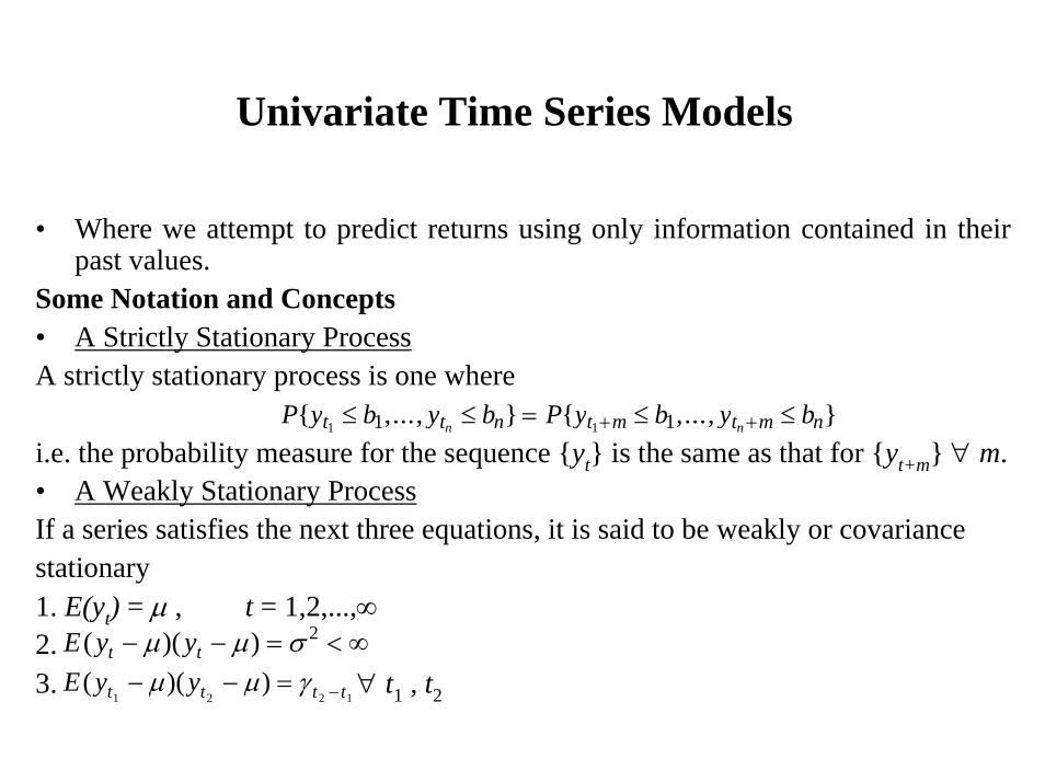
Univariate Time Series Models

• Where we attempt to predict returns using only information contained in their past values.

Some Notation and Concepts• A Strictly Stationary ProcessA strictly stationary process is one where

i.e. the probability measure for the sequence yt is the same as that for yt+m ∀ m. • A Weakly Stationary ProcessIf a series satisfies the next three equations, it is said to be weakly or covariancestationary1. E(yt) = µ , t = 1,2,...,∞2.3. ∀ t1 , t2

P y b y b P y b y bt t n t m t m nn n ,..., ,...,

1 11 1≤ ≤ = ≤ ≤+ +

E y yt t t t( )( )1 2 2 1

− − = −µ µ γE y yt t( )( )− − = < ∞µ µ σ 2

Univariate Time Series Models (cont’d)

• So if the process is covariance stationary, all the variances are the same and all the covariances depend on the difference between t1 and t2. The moments

, s = 0,1,2, ...are known as the covariance function.

• The covariances, γs, are known as autocovariances.

• However, the value of the autocovariances depend on the units of measurement of yt.

• It is thus more convenient to use the autocorrelations which are the autocovariances normalised by dividing by the variance:

, s = 0,1,2, ...

• If we plot τs against s=0,1,2,... then we obtain the autocorrelation function orcorrelogram.

τ γγs

s=0

E y E y y E yt t t s t s s( ( ))( ( ))− − =+ + γ

A White Noise Process

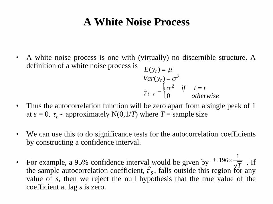
• A white noise process is one with (virtually) no discernible structure. A definition of a white noise process is

• Thus the autocorrelation function will be zero apart from a single peak of 1 at s = 0. τs ∼ approximately N(0,1/T) where T = sample size

• We can use this to do significance tests for the autocorrelation coefficients by constructing a confidence interval.

• For example, a 95% confidence interval would be given by . If the sample autocorrelation coefficient, , falls outside this region for any value of s, then we reject the null hypothesis that the true value of the coefficient at lag s is zero.

E yVar y

if t rotherwise

t

t

t r

( )( )

==

= =⎧⎨⎩−

µσ

γ σ

2

2

0

τ sT1196. ×±

Joint Hypothesis Tests

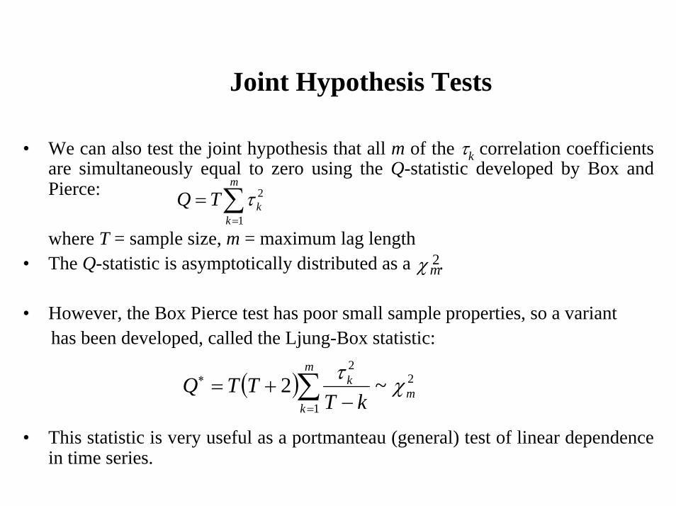
• We can also test the joint hypothesis that all m of the τk correlation coefficients are simultaneously equal to zero using the Q-statistic developed by Box and Pierce:

where T = sample size, m = maximum lag length• The Q-statistic is asymptotically distributed as a .

• However, the Box Pierce test has poor small sample properties, so a varianthas been developed, called the Ljung-Box statistic:

• This statistic is very useful as a portmanteau (general) test of linear dependence in time series.

χ m2

∑=

=m

kkTQ

1

2τ

( ) 2

1

2

~2 m

m

k

k

kTTTQ χτ∑

=

∗

−+=

An ACF Example

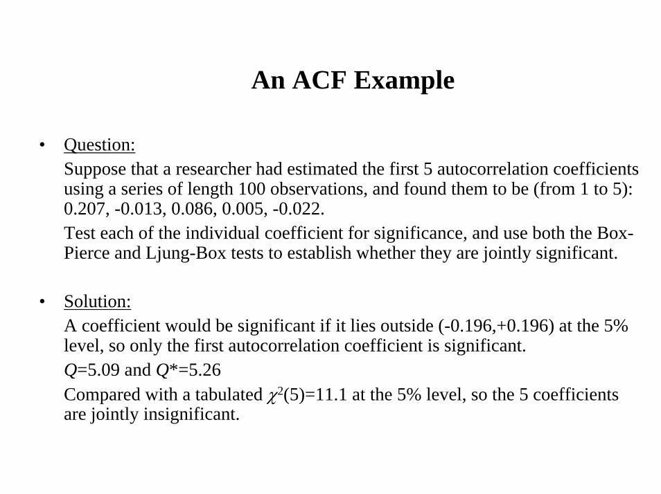
• Question:Suppose that a researcher had estimated the first 5 autocorrelation coefficients using a series of length 100 observations, and found them to be (from 1 to 5): 0.207, -0.013, 0.086, 0.005, -0.022.Test each of the individual coefficient for significance, and use both the Box-Pierce and Ljung-Box tests to establish whether they are jointly significant.

• Solution:A coefficient would be significant if it lies outside (-0.196,+0.196) at the 5% level, so only the first autocorrelation coefficient is significant.Q=5.09 and Q*=5.26Compared with a tabulated χ2(5)=11.1 at the 5% level, so the 5 coefficients are jointly insignificant.

Moving Average Processes

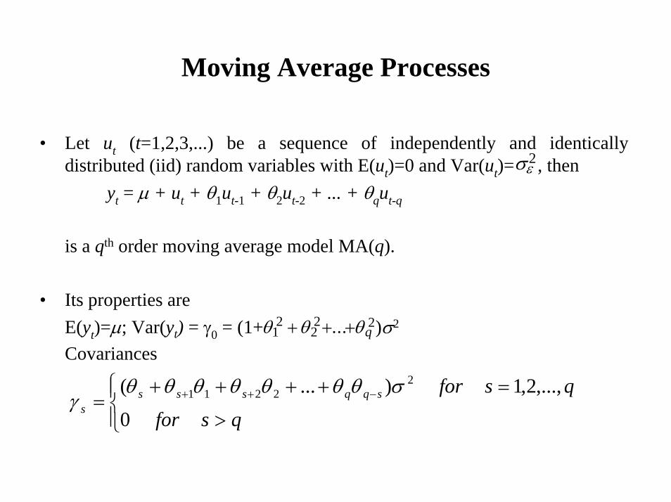
• Let ut (t=1,2,3,...) be a sequence of independently and identically distributed (iid) random variables with E(ut)=0 and Var(ut)= , then

yt = µ + ut + θ1ut-1 + θ2ut-2 + ... + θqut-q

is a qth order moving average model MA(q).

• Its properties are E(yt)=µ; Var(yt) = γ0 = (1+ )σ2

Covariances

σε2

θ θ θ12

22 2+ + +... q

⎪⎩

⎪⎨⎧

>

=++++= −++

qsfor

qsforsqqssss

0

,...,2,1)...( 22211 σθθθθθθθ

γ

Example of an MA Problem

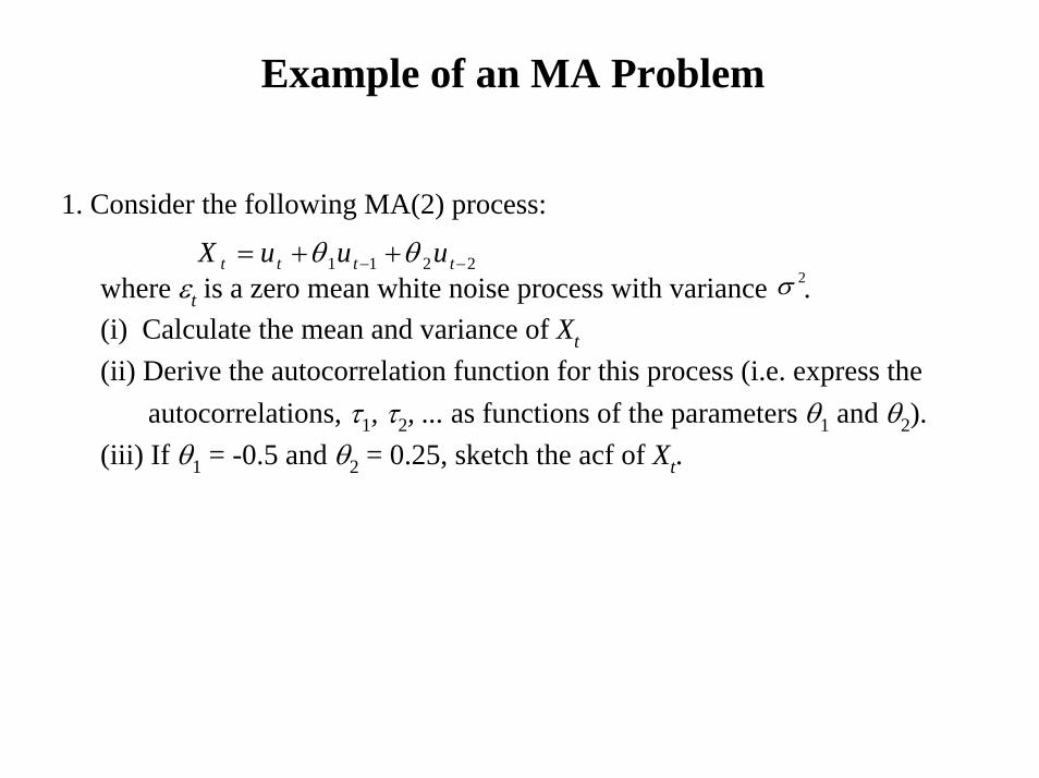
1. Consider the following MA(2) process:

where εt is a zero mean white noise process with variance .(i) Calculate the mean and variance of Xt

(ii) Derive the autocorrelation function for this process (i.e. express theautocorrelations, τ1, τ2, ... as functions of the parameters θ1 and θ2).

(iii) If θ1 = -0.5 and θ2 = 0.25, sketch the acf of Xt.

2211 −− ++= tttt uuuX θθ2σ

Solution

(i) If E(ut)=0, then E(ut-i)=0 ∀ i.So

E(Xt) = E(ut + θ1ut-1+ θ2ut-2)= E(ut)+ θ1E(ut-1)+ θ2E(ut-2)=0

Var(Xt) = E[Xt-E(Xt)][Xt-E(Xt)]but E(Xt) = 0, soVar(Xt) = E[(Xt)(Xt)]

= E[(ut + θ1ut-1+ θ2ut-2)(ut + θ1ut-1+ θ2ut-2)]= E[ +cross-products]

But E[cross-products]=0 since Cov(ut,ut-s)=0 for s≠0.

22

22

21

21

2−− ++ ttt uuu θθ

Solution (cont’d)

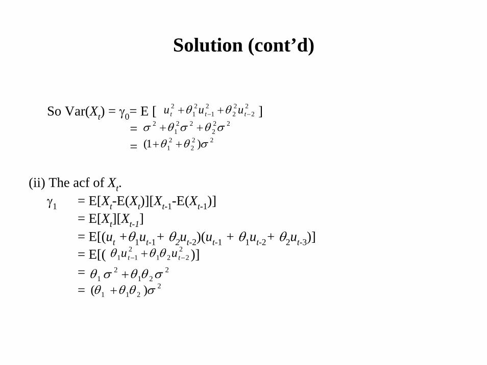
So Var(Xt) = γ0= E [ ]= =

(ii) The acf of Xt. γ1 = E[Xt-E(Xt)][Xt-1-E(Xt-1)]

= E[Xt][Xt-1]= E[(ut +θ1ut-1+ θ2ut-2)(ut-1 + θ1ut-2+ θ2ut-3)]= E[( )]= =

22

22

21

21

2−− ++ ttt uuu θθ

222

221

2 σθσθσ ++22

22

1 )1( σθθ ++

2221

211 −− + tt uu θθθ

221

21 σθθσθ +

2211 )( σθθθ +

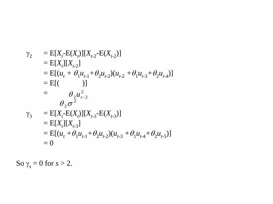
γ2 = E[Xt-E(Xt)][Xt-2-E(Xt-2)]= E[Xt][Xt-2]= E[(ut + θ1ut-1+θ2ut-2)(ut-2 +θ1ut-3+θ2ut-4)]= E[( )]=

γ3 = E[Xt-E(Xt)][Xt-3-E(Xt-3)]= E[Xt][Xt-3]= E[(ut +θ1ut-1+θ2ut-2)(ut-3 +θ1ut-4+θ2ut-5)]= 0

So γs = 0 for s > 2.

222 −tuθ

22σθ

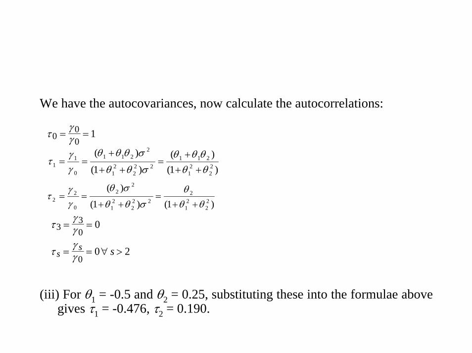
We have the autocovariances, now calculate the autocorrelations:

(iii) For θ1 = -0.5 and θ2 = 0.25, substituting these into the formulae above gives τ1 = -0.476, τ2 = 0.190.

τγγ0

00

1= =

τγγ3

30

0= =

τγγs

s s= = ∀ >0

0 2

)1()(

)1(

)(22

21

21122

22

1

2211

0

11 θθ

θθθσθθ

σθθθγγ

τ++

+=

++

+==

)1()1(

)(22

21

222

22

1

22

0

22 θθ

θσθθ

σθγγ

τ++

=++

==

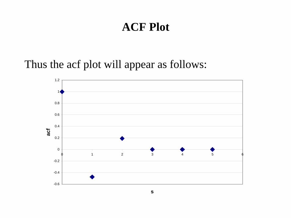
ACF Plot

Thus the acf plot will appear as follows:

-0.6

-0.4

-0.2

0

0.2

0.4

0.6

0.8

1

1.2

0 1 2 3 4 5 6

s

acf

Autoregressive Processes

• An autoregressive model of order p, an AR(p) can be expressed as

• Or using the lag operator notation:Lyt = yt-1 Liyt = yt-i

• or

or where .φ φ φ φ( ) ( ... )L L L Lpp= − + +1 1 2

2

tptpttt uyyyy +++++= −−− φφφµ ...2211

∑=

− ++=p

ititit uyy

1φµ

∑=

++=p

itt

iit uyLy

1φµ

tt uyL += µφ )(

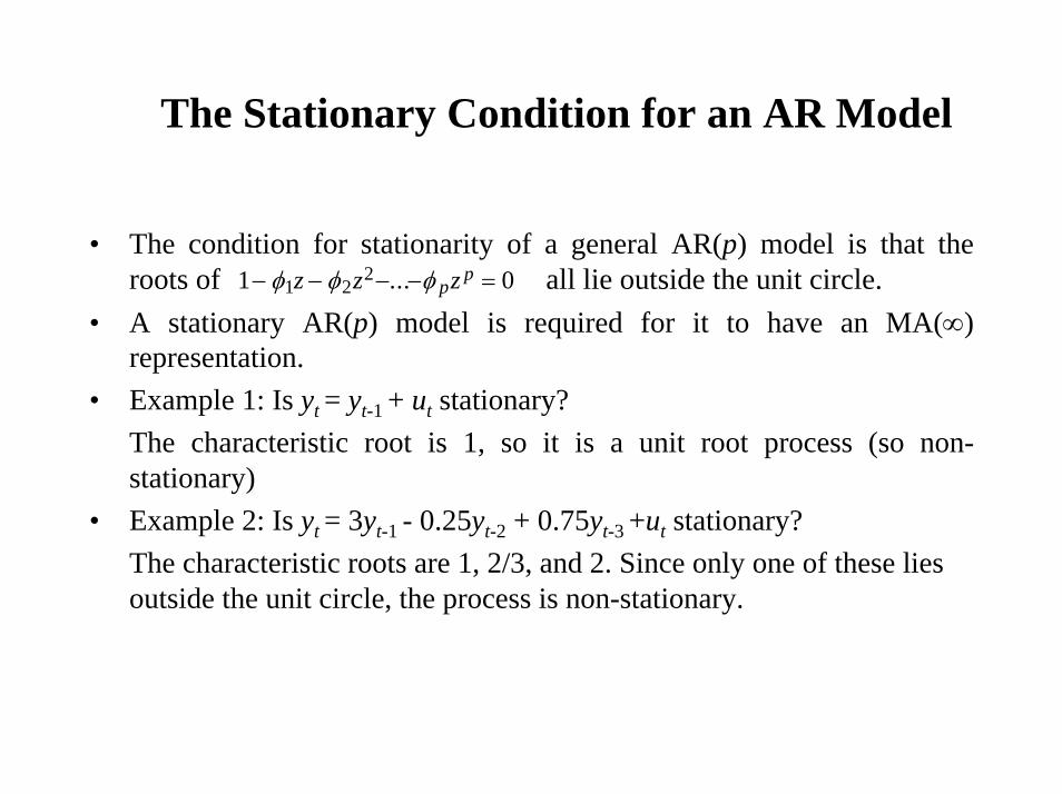
The Stationary Condition for an AR Model

• The condition for stationarity of a general AR(p) model is that the roots of all lie outside the unit circle.

• A stationary AR(p) model is required for it to have an MA(∞) representation.

• Example 1: Is yt = yt-1 + ut stationary?The characteristic root is 1, so it is a unit root process (so non-stationary)

• Example 2: Is yt = 3yt-1 - 0.25yt-2 + 0.75yt-3 +ut stationary?The characteristic roots are 1, 2/3, and 2. Since only one of these lies outside the unit circle, the process is non-stationary.

1 01 22− − − − =φ φ φz z zp

p...

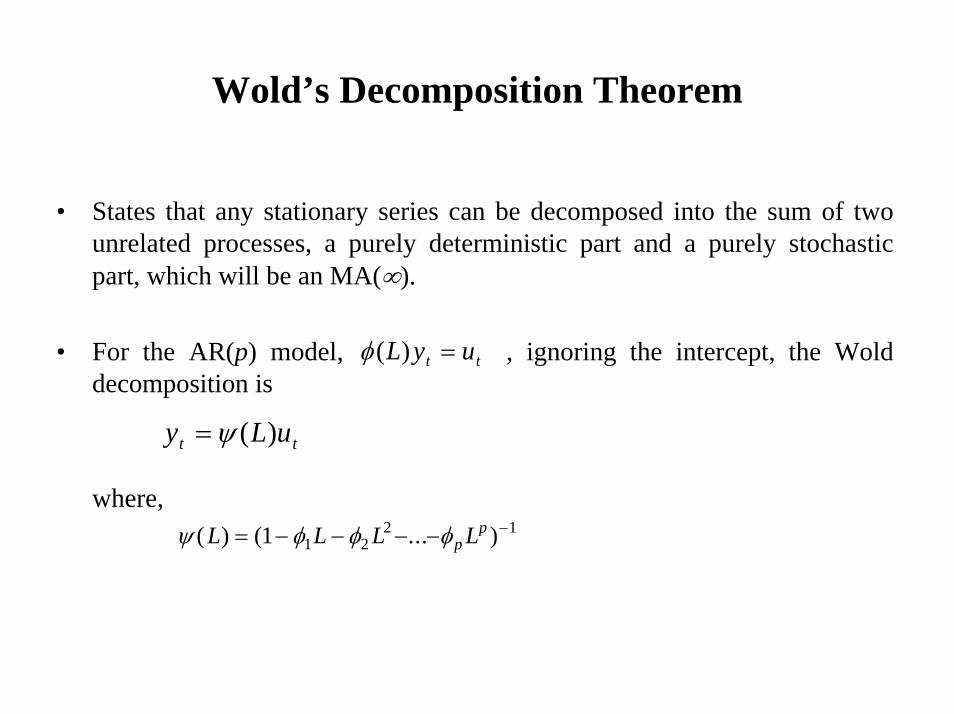
Wold’s Decomposition Theorem

• States that any stationary series can be decomposed into the sum of two unrelated processes, a purely deterministic part and a purely stochastic part, which will be an MA(∞).

• For the AR(p) model, , ignoring the intercept, the Wold decomposition is

where, ψ φ φ φ( ) ( ... )L L L Lp

p= − − − − −1 1 22 1

tt uyL =)(φ

tt uLy )(ψ=

The Moments of an Autoregressive Process

• The moments of an autoregressive process are as follows. The mean is given by

• The autocovariances and autocorrelation functions can be obtained by solving what are known as the Yule-Walker equations:

• If the AR model is stationary, the autocorrelation function will decay exponentially to zero.

ptyE

φφφφ

−−−−=

...1)(

21

0

pppp

pp

pp

φφτφττ

φτφφττ

φτφτφτ

+++=

+++=

+++=

−−

−

−

...

...

...

2211

22112

12111

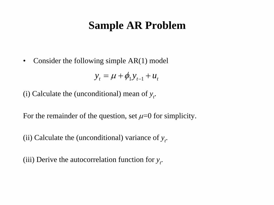
Sample AR Problem

• Consider the following simple AR(1) model

(i) Calculate the (unconditional) mean of yt.

For the remainder of the question, set µ=0 for simplicity.

(ii) Calculate the (unconditional) variance of yt.

(iii) Derive the autocorrelation function for yt.

ttt uyy ++= −11φµ

Solution

(i) Unconditional mean: E(yt) = E(µ+φ1yt-1)

=µ +φ1E(yt-1)But also

So E(yt)= µ +φ1 (µ +φ1E(yt-2))= µ +φ1 µ +φ1

2 E(yt-2))

E(yt) = µ +φ1 µ +φ12 E(yt-2))

= µ +φ1 µ +φ12 (µ +φ1E(yt-3))

= µ +φ1 µ +φ12 µ +φ1

3 E(yt-3)

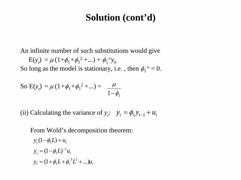
Solution (cont’d)

An infinite number of such substitutions would giveE(yt) = µ (1+φ1+φ1

2 +...) + φ1∞y0

So long as the model is stationary, i.e. , then φ1∞ = 0.

So E(yt) = µ (1+φ1+φ12 +...) =

(ii) Calculating the variance of yt:

From Wold’s decomposition theorem:

11 φµ−

ttt uyy += −11φ

tt uLy =− )1( 1φ

tt uLy 11 )1( −−= φ

tt uLLy ...)1( 2211 +++= φφ

Solution (cont’d)

So long as , this will converge.

Var(yt) = E[yt-E(yt)][yt-E(yt)]but E(yt) = 0, since we are setting µ = 0.Var(yt) = E[(yt)(yt)]= E[ ]= E[= E[= = =

11 <φ...2

2111 +++= −− tttt uuuy φφ

( )( ).... 22

11122

111 ++++++ −−−− tttttt uuuuuu φφφφ)]...( 2

24

12

12

12 productscrossuuu ttt −++++ −− φφ

...)]( 22

41

21

21

2 +++ −− ttt uuu φφ...24

122

12 +++ uuu σφσφσ

...)1( 41

21

2 +++ φφσ u

)1( 21

2

φσ−

u

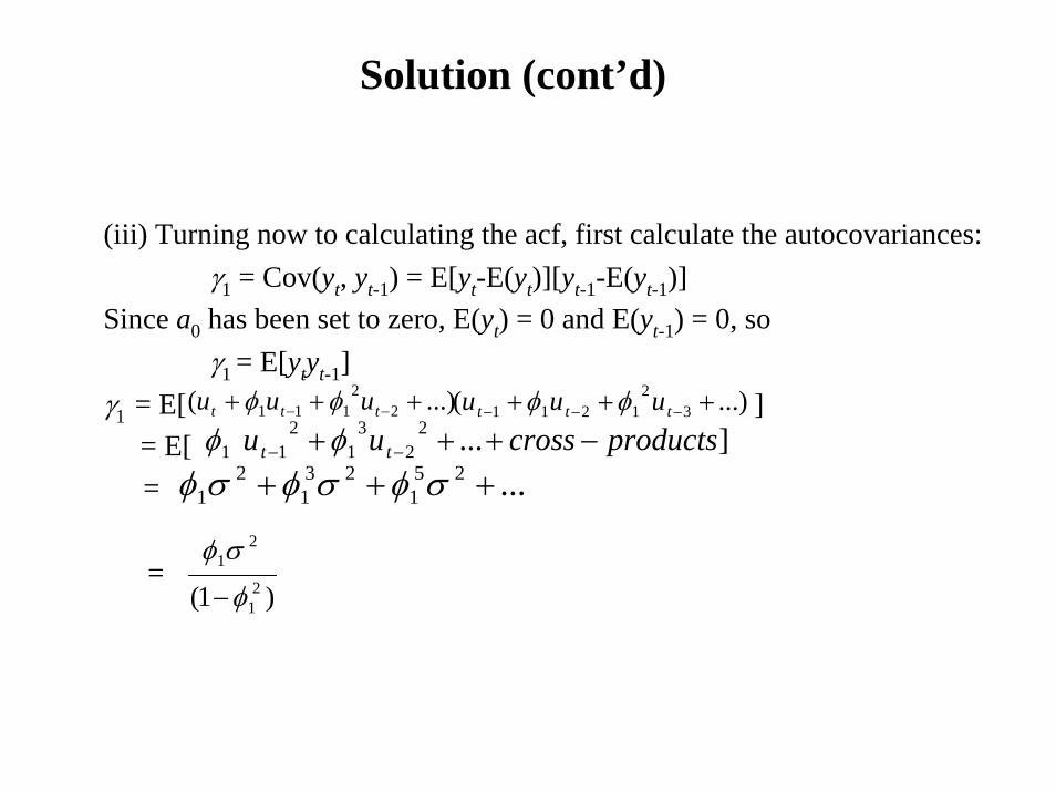
Solution (cont’d)

(iii) Turning now to calculating the acf, first calculate the autocovariances:γ1 = Cov(yt, yt-1) = E[yt-E(yt)][yt-1-E(yt-1)]

Since a0 has been set to zero, E(yt) = 0 and E(yt-1) = 0, soγ1 = E[ytyt-1]

γ1 = E[ ] = E[ =

=

...)( 22

111 +++ −− ttt uuu φφ ...)( 32

1211 +++ −−− ttt uuu φφ]...2

23

12

11 productscrossuu tt −+++ −− φφ...25

123

12

1 +++ σφσφσφ

)1( 21

21

φ

σφ

−

Solution (cont’d)

For the second autocorrelation coefficient,γ2 = Cov(yt, yt-2) = E[yt-E(yt)][yt-2-E(yt-2)]

Using the same rules as applied above for the lag 1 covarianceγ2 = E[ytyt-2]

= E[ ] = E[==

=

...)( 22

111 +++ −− ttt uuu φφ ...)( 42

1312 +++ −−− ttt uuu φφ]...2

34

12

22

1 productscrossuu tt −+++ −− φφ...24

122

1 ++ σφσφ...)1( 4

12

122

1 +++ φφσφ

)1( 21

221

φ

σφ

−

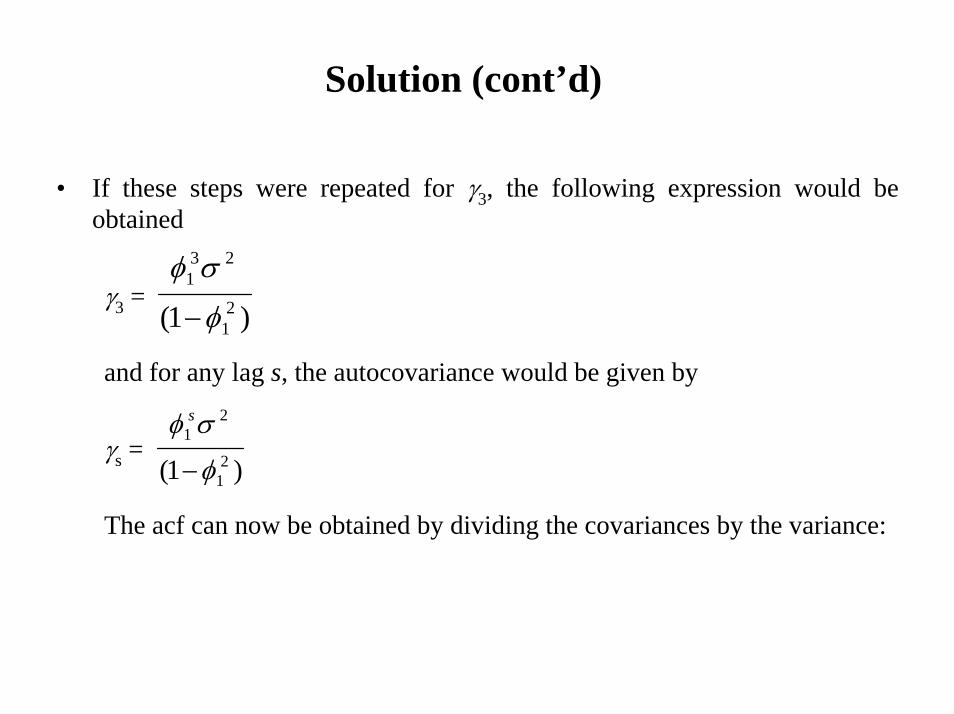
Solution (cont’d)

• If these steps were repeated for γ3, the following expression would be obtained

γ3 =

and for any lag s, the autocovariance would be given by

γs =

The acf can now be obtained by dividing the covariances by the variance:

)1( 21

231

φ

σφ

−

)1( 21

21

φ

σφ

−

s

Solution (cont’d)

τ0 =

τ1 = τ2 =

τ3 = …τs =

10

0 =γγ

1

21

2

21

21

0

1

)1(

)1(φ

φ

σ

φ

σφ

γγ

=

⎟⎟⎟

⎠

⎞

⎜⎜⎜

⎝

⎛

−

⎟⎟⎟

⎠

⎞

⎜⎜⎜

⎝

⎛

−= 2

1

21

2

21

221

0

2

)1(

)1(φ

φ

σ

φ

σφ

γγ

=

⎟⎟⎟

⎠

⎞

⎜⎜⎜

⎝

⎛

−

⎟⎟⎟

⎠

⎞

⎜⎜⎜

⎝

⎛

−=

31φ

s1φ

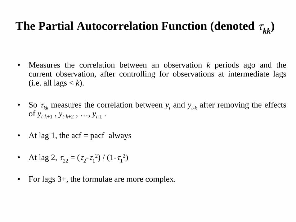
The Partial Autocorrelation Function (denoted τkk)

• Measures the correlation between an observation k periods ago and the current observation, after controlling for observations at intermediate lags (i.e. all lags < k).

• So τkk measures the correlation between yt and yt-k after removing the effects of yt-k+1 , yt-k+2 , …, yt-1 .

• At lag 1, the acf = pacf always

• At lag 2, τ22 = (τ2-τ12) / (1-τ1

2)

• For lags 3+, the formulae are more complex.

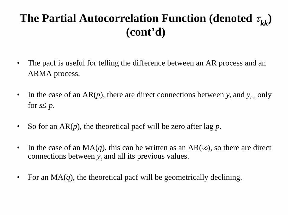
The Partial Autocorrelation Function (denoted τkk)(cont’d)

• The pacf is useful for telling the difference between an AR process and anARMA process.

• In the case of an AR(p), there are direct connections between yt and yt-s onlyfor s≤ p.

• So for an AR(p), the theoretical pacf will be zero after lag p.

• In the case of an MA(q), this can be written as an AR(∞), so there are direct connections between yt and all its previous values.

• For an MA(q), the theoretical pacf will be geometrically declining.

ARMA Processes

• By combining the AR(p) and MA(q) models, we can obtain an ARMA(p,q) model:

where

and

or

with

φ φ φ φ( ) ...L L L Lpp= − − − −1 1 2

2

qqLLLL θθθθ ++++= ...1)( 2

21

tt uLyL )()( θµφ +=

tqtqttptpttt uuuuyyyy +++++++++= −−−−−− θθθφφφµ ...... 22112211

stuuEuEuE sttt ≠=== ,0)(;)(;0)( 22 σ

The Invertibility Condition

• Similar to the stationarity condition, we typically require the MA(q) part of the model to have roots of θ(z)=0 greater than one in absolute value.

• The mean of an ARMA series is given by

• The autocorrelation function for an ARMA process will display combinations of behaviour derived from the AR and MA parts, but for lags beyond q, the acf will simply be identical to the individual AR(p) model.

E ytp

( )...

=− − − −

µφ φ φ1 1 2

Summary of the Behaviour of the acf for AR and MA Processes

An autoregressive process has• a geometrically decaying acf• number of spikes of pacf = AR order

A moving average process has• Number of spikes of acf = MA order• a geometrically decaying pacf

Some sample acf and pacf plots for standard processes

The acf and pacf are not produced analytically from the relevant formulae for a model of that type, but rather are estimated using 100,000 simulated observations with disturbances drawn from a normal distribution.

ACF and PACF for an MA(1) Model: yt = – 0.5ut-1 + ut

-0.45

-0.4

-0.35

-0.3

-0.25

-0.2

-0.15

-0.1

-0.05

0

0.05

1 2 3 4 5 6 7 8 9 10

Lag

acfa

nd p

acf

acfpacf

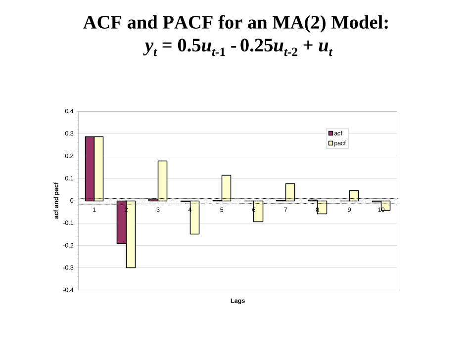
ACF and PACF for an MA(2) Model:yt = 0.5ut-1 - 0.25ut-2 + ut

-0.4

-0.3

-0.2

-0.1

0

0.1

0.2

0.3

0.4

1 2 3 4 5 6 7 8 9 10

Lags

acf a

nd p

acf

acfpacf

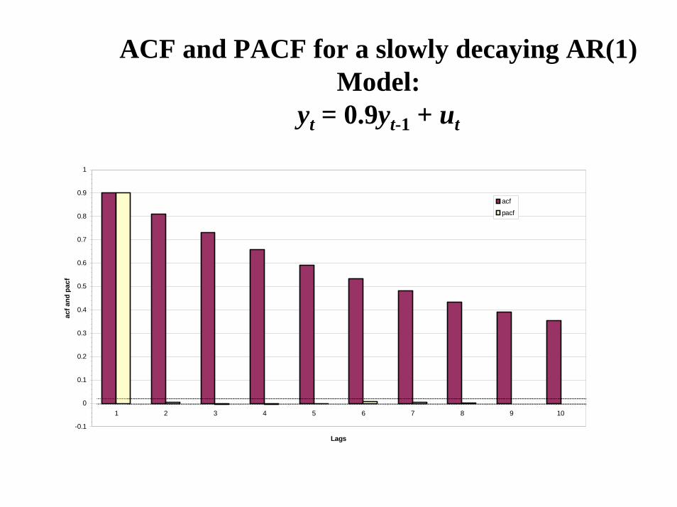
ACF and PACF for a slowly decaying AR(1) Model:

yt = 0.9yt-1 + ut

-0.1

0

0.1

0.2

0.3

0.4

0.5

0.6

0.7

0.8

0.9

1

1 2 3 4 5 6 7 8 9 10

Lags

acf a

nd p

acf

acf

pacf

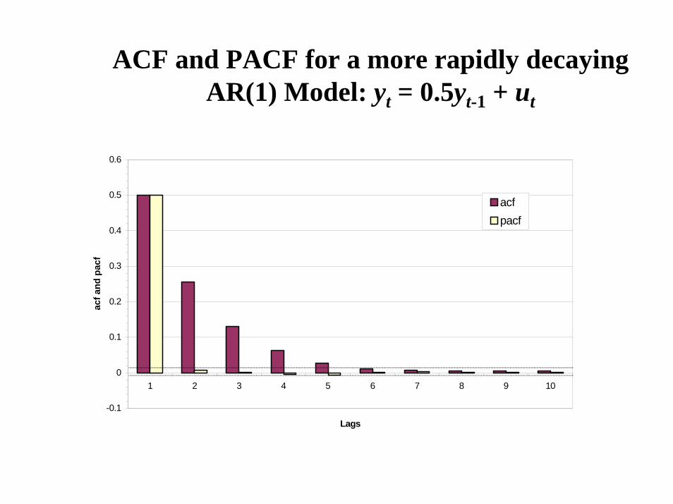
ACF and PACF for a more rapidly decaying AR(1) Model: yt = 0.5yt-1 + ut

-0.1

0

0.1

0.2

0.3

0.4

0.5

0.6

1 2 3 4 5 6 7 8 9 10

Lags

acf a

nd p

acf

acfpacf

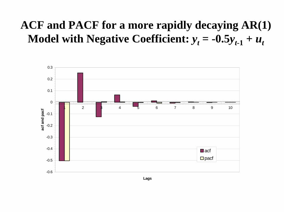
ACF and PACF for a more rapidly decaying AR(1) Model with Negative Coefficient: yt = -0.5yt-1 + ut

-0.6

-0.5

-0.4

-0.3

-0.2

-0.1

0

0.1

0.2

0.3

1 2 3 4 5 6 7 8 9 10

Lags

acf a

nd p

acf

acfpacf

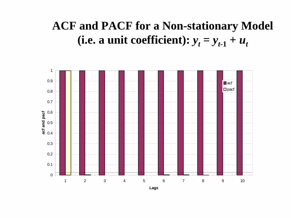
ACF and PACF for a Non-stationary Model (i.e. a unit coefficient): yt = yt-1 + ut

0

0.1

0.2

0.3

0.4

0.5

0.6

0.7

0.8

0.9

1

1 2 3 4 5 6 7 8 9 10

Lags

acf a

nd p

acf

acfpacf

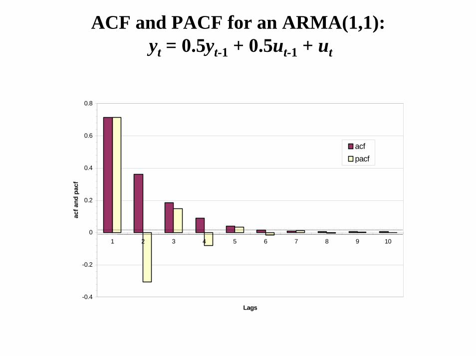
ACF and PACF for an ARMA(1,1):yt = 0.5yt-1 + 0.5ut-1 + ut

-0.4

-0.2

0

0.2

0.4

0.6

0.8

1 2 3 4 5 6 7 8 9 10

Lags

acf a

nd p

acf

acfpacf

Building ARMA Models - The Box Jenkins Approach

• Box and Jenkins (1970) were the first to approach the task of estimating an ARMA model in a systematic manner. There are 3 steps to their approach:1. Identification2. Estimation3. Model diagnostic checking

Step 1:- Involves determining the order of the model.- Use of graphical procedures- A better procedure is now available

Building ARMA Models - The Box Jenkins Approach (cont’d)

Step 2:- Estimation of the parameters- Can be done using least squares or maximum likelihood dependingon the

model.

Step 3:- Model checking

Box and Jenkins suggest 2 methods:- deliberate overfitting- residual diagnostics

Some More Recent Developments in ARMA Modelling

• Identification would typically not be done using acf’s.• We want to form a parsimonious model.

• Reasons:- variance of estimators is inversely proportional to the number of degrees offreedom.

- models which are profligate might be inclined to fit to data specific features

• This gives motivation for using information criteria, which embody 2 factors- a term which is a function of the RSS- some penalty for adding extra parameters

• The object is to choose the number of parameters which minimises the information criterion.

Information Criteria for Model Selection

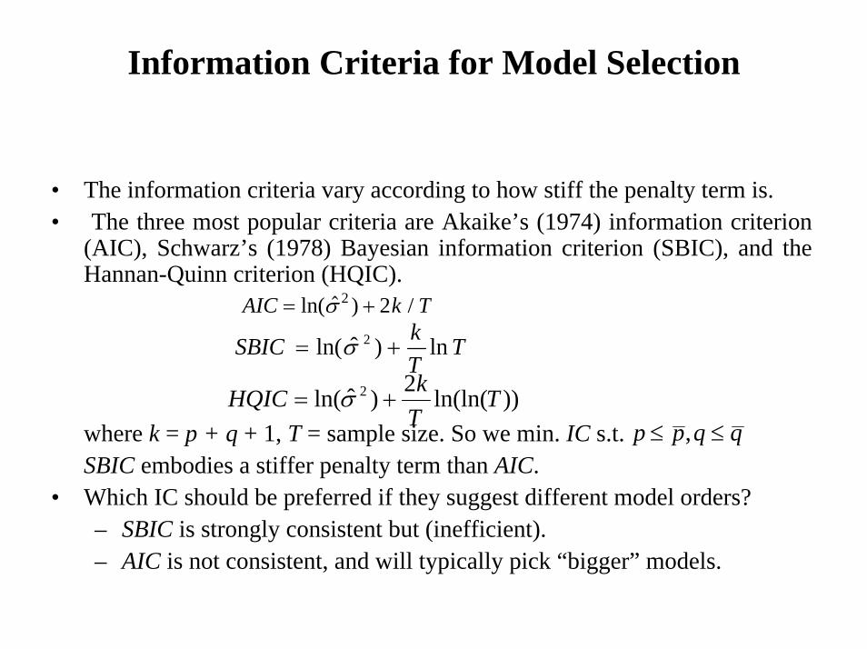
• The information criteria vary according to how stiff the penalty term is. • The three most popular criteria are Akaike’s (1974) information criterion

(AIC), Schwarz’s (1978) Bayesian information criterion (SBIC), and the Hannan-Quinn criterion (HQIC).

where k = p + q + 1, T = sample size. So we min. IC s.t.SBIC embodies a stiffer penalty term than AIC.

• Which IC should be preferred if they suggest different model orders?– SBIC is strongly consistent but (inefficient).– AIC is not consistent, and will typically pick “bigger” models.

AIC k T= +ln( ) /σ 2 2

p p q q≤ ≤,

TTkSBIC ln)ˆln( 2 += σ

))ln(ln(2)ˆln( 2 TTkHQIC += σ

ARIMA Models

• As distinct from ARMA models. The I stands for integrated.

• An integrated autoregressive process is one with a characteristic root on the unit circle.

• Typically researchers difference the variable as necessary and then build an ARMA model on those differenced variables.

• An ARMA(p,q) model in the variable differenced d times is equivalent to an ARIMA(p,d,q) model on the original data.

Forecasting in Econometrics

• Forecasting = prediction.• An important test of the adequacy of a model.e.g.- Forecasting tomorrow’s return on a particular share- Forecasting the price of a house given its characteristics- Forecasting the riskiness of a portfolio over the next year- Forecasting the volatility of bond returns

• We can distinguish two approaches:- Econometric (structural) forecasting - Time series forecasting

• The distinction between the two types is somewhat blurred (e.g, VARs).

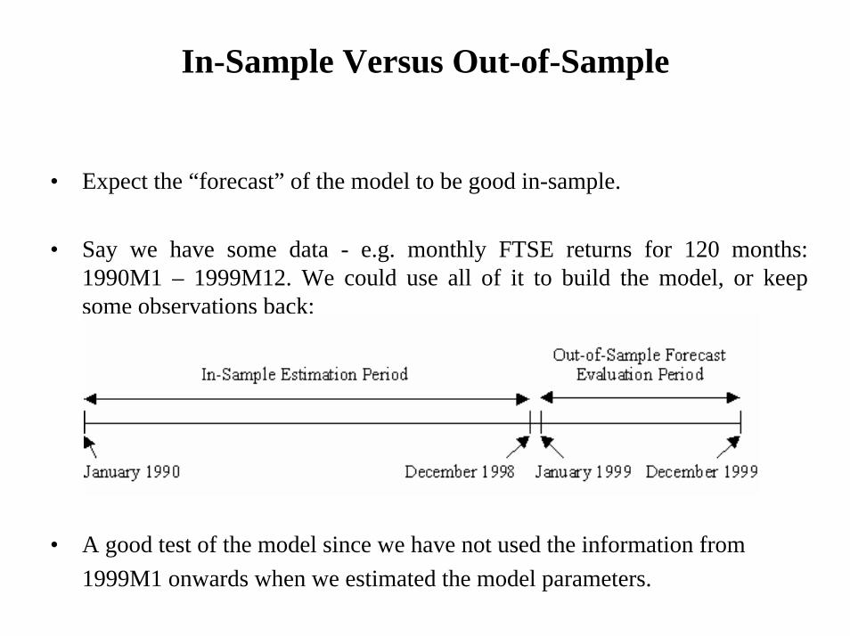
In-Sample Versus Out-of-Sample

• Expect the “forecast” of the model to be good in-sample.

• Say we have some data - e.g. monthly FTSE returns for 120 months: 1990M1 – 1999M12. We could use all of it to build the model, or keep some observations back:

• A good test of the model since we have not used the information from1999M1 onwards when we estimated the model parameters.

How to produce forecasts

• Multi-step ahead versus single-step ahead forecasts• Recursive versus rolling windows

• To understand how to construct forecasts, we need the idea of conditional expectations:

E(yt+1 | Ωt )

• We cannot forecast a white noise process: E(ut+s | Ωt ) = 0 ∀ s > 0.

• The two simplest forecasting “methods”1. Assume no change : f(yt+s) = yt

2. Forecasts are the long term average f(yt+s) = y

Models for Forecasting

• Structural modelse.g. y = Xβ + u

To forecast y, we require the conditional expectation of its future value:

=But what are etc.? We could use , so

= !!

tktktt uxxy ++++= βββ …221

( ) ( )tktkttt uxxEyE ++++=Ω − βββ …2211

( ) ( )ktkt xExE βββ +++ …221

)( 2txΕ 2x

( ) kkt xxyE βββ +++= …221y

Models for Forecasting (cont’d)

• Time Series ModelsThe current value of a series, yt, is modelled as a function only of its previous values and the current value of an error term (and possibly previous values of the error term).

• Models include:• simple unweighted averages• exponentially weighted averages• ARIMA models• Non-linear models – e.g. threshold models, GARCH, bilinear models, etc.

Forecasting with ARMA Models

The forecasting model typically used is of the form:

where ft,s = yt+s , s≤ 0; ut+s = 0, s > 0= ut+s , s ≤ 0

∑∑=

−+=

− ++=q

jjstj

p

iistist uff

11,, θφµ

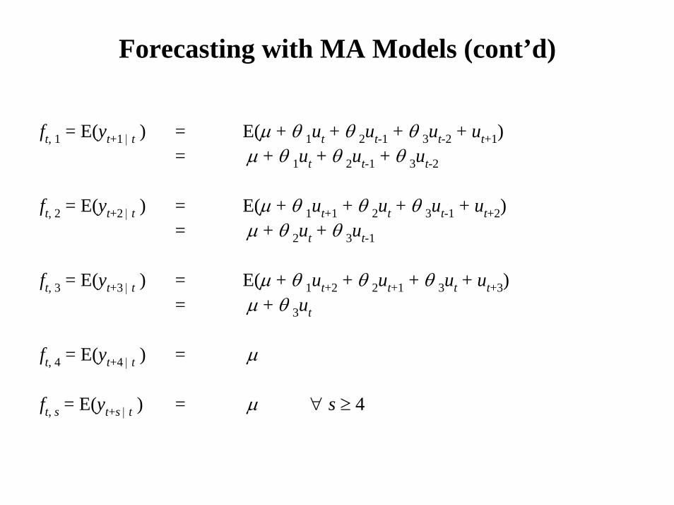
Forecasting with MA Models

• An MA(q) only has memory of q.

e.g. say we have estimated an MA(3) model:

yt = µ + θ1ut-1 + θ 2ut-2 + θ 3ut-3 + ut

yt+1 = µ + θ 1ut + θ 2ut-1 + θ 3ut-2 + ut+1

yt+2 = µ + θ 1ut+1 + θ 2ut + θ 3ut-1 + ut+2

yt+3 = µ + θ 1ut+2 + θ 2ut+1 + θ 3ut + ut+3

• We are at time t and we want to forecast 1,2,..., s steps ahead.

• We know yt , yt-1, ..., and ut , ut-1

Forecasting with MA Models (cont’d)

ft, 1 = E(yt+1 | t ) = E(µ + θ 1ut + θ 2ut-1 + θ 3ut-2 + ut+1)= µ + θ 1ut + θ 2ut-1 + θ 3ut-2

ft, 2 = E(yt+2 | t ) = E(µ + θ 1ut+1 + θ 2ut + θ 3ut-1 + ut+2)= µ + θ 2ut + θ 3ut-1

ft, 3 = E(yt+3 | t ) = E(µ + θ 1ut+2 + θ 2ut+1 + θ 3ut + ut+3)= µ + θ 3ut

ft, 4 = E(yt+4 | t ) = µ

ft, s = E(yt+s | t ) = µ ∀ s ≥ 4

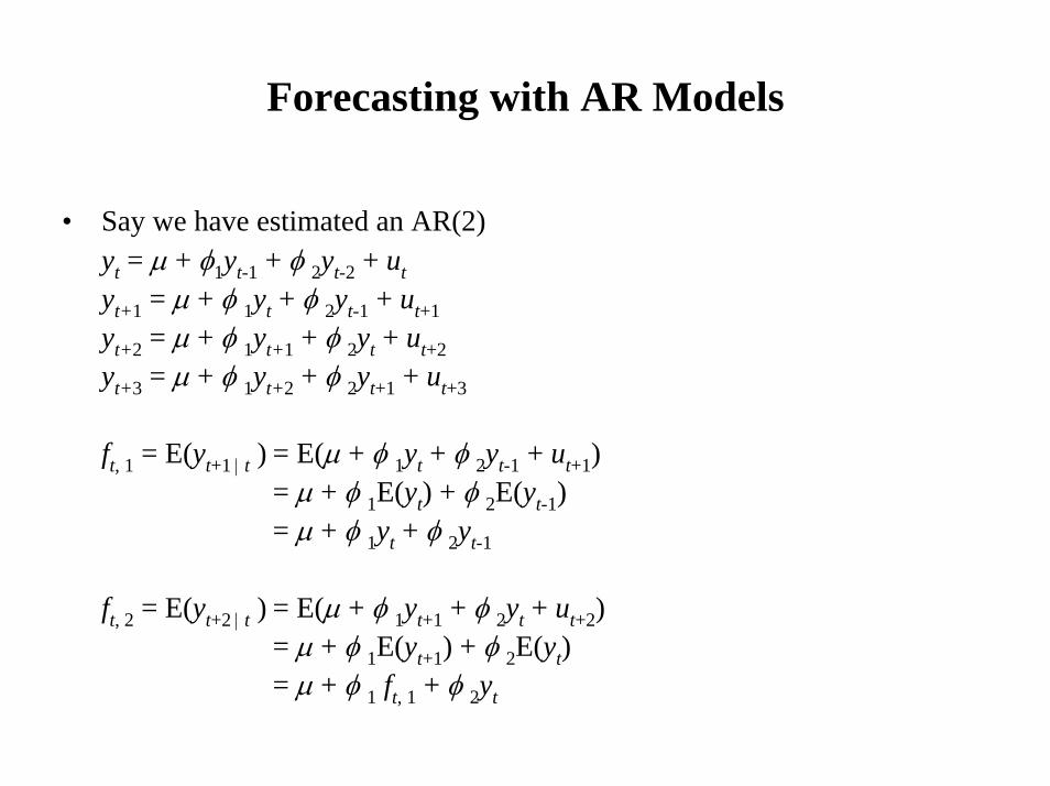
Forecasting with AR Models

• Say we have estimated an AR(2)yt = µ + φ1yt-1 + φ 2yt-2 + utyt+1 = µ + φ 1yt + φ 2yt-1 + ut+1yt+2 = µ + φ 1yt+1 + φ 2yt + ut+2yt+3 = µ + φ 1yt+2 + φ 2yt+1 + ut+3

ft, 1 = E(yt+1 | t ) = E(µ + φ 1yt + φ 2yt-1 + ut+1)= µ + φ 1E(yt) + φ 2E(yt-1)= µ + φ 1yt + φ 2yt-1

ft, 2 = E(yt+2 | t ) = E(µ + φ 1yt+1 + φ 2yt + ut+2)= µ + φ 1E(yt+1) + φ 2E(yt)= µ + φ 1 ft, 1 + φ 2yt

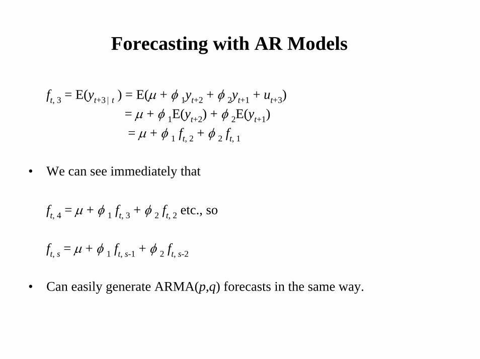
Forecasting with AR Models

ft, 3 = E(yt+3 | t ) = E(µ + φ 1yt+2 + φ 2yt+1 + ut+3)= µ + φ 1E(yt+2) + φ 2E(yt+1)= µ + φ 1 ft, 2 + φ 2 ft, 1

• We can see immediately that

ft, 4 = µ + φ 1 ft, 3 + φ 2 ft, 2 etc., so

ft, s = µ + φ 1 ft, s-1 + φ 2 ft, s-2

• Can easily generate ARMA(p,q) forecasts in the same way.

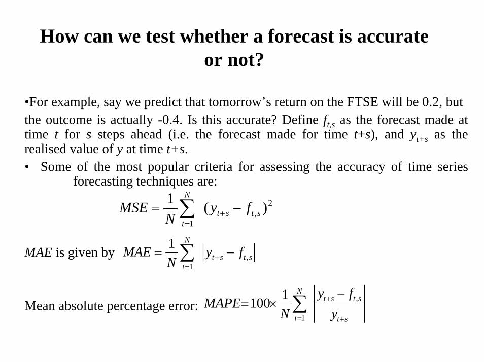
How can we test whether a forecast is accurate or not?

•For example, say we predict that tomorrow’s return on the FTSE will be 0.2, butthe outcome is actually -0.4. Is this accurate? Define ft,s as the forecast made at time t for s steps ahead (i.e. the forecast made for time t+s), and yt+s as the realised value of y at time t+s.• Some of the most popular criteria for assessing the accuracy of time series

forecasting techniques are:

MAE is given by

Mean absolute percentage error:

2,

1)(1

stst

N

tfy

NMSE −= +

=∑

stst

N

tfy

NMAE ,

1

1−= +

=∑

st

ststN

t yfy

NMAPE

+

+

=

−×= ∑ ,

1

1100

How can we test whether a forecast is accurate or not? (cont’d)

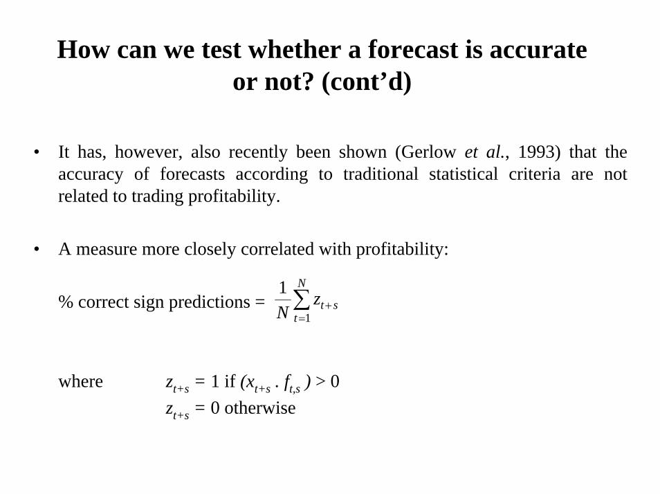
• It has, however, also recently been shown (Gerlow et al., 1993) that the accuracy of forecasts according to traditional statistical criteria are not related to trading profitability.

• A measure more closely correlated with profitability:

% correct sign predictions =

where zt+s = 1 if (xt+s . ft,s ) > 0zt+s = 0 otherwise

∑=

+

N

tstz

N 1

1

Forecast Evaluation Example

• Given the following forecast and actual values, calculate the MSE, MAE and percentage of correct sign predictions:

• MSE = 0.079, MAE = 0.180, % of correct sign predictions = 40

Steps Ahead Forecast Actual

1 0.20 -0.40 2 0.15 0.20 3 0.10 0.10 4 0.06 -0.10 5 0.04 -0.05

What factors are likely to lead to a good forecasting model?

• “signal” versus “noise”

• “data mining” issues

• simple versus complex models

• financial or economic theory

Statistical Versus Economic or Financial loss functions

• Statistical evaluation metrics may not be appropriate.• How well does the forecast perform in doing the job we wanted it for?

Limits of forecasting: What can and cannot be forecast?• All statistical forecasting models are essentially extrapolative

• Forecasting models are prone to break down around turning points

• Series subject to structural changes or regime shifts cannot be forecast

• Predictive accuracy usually declines with forecasting horizon

• Forecasting is not a substitute for judgement

Back to the original question: why forecast?

• Why not use “experts” to make judgemental forecasts?• Judgemental forecasts bring a different set of problems:

e.g., psychologists have found that expert judgements are prone to the following biases:

– over-confidence– inconsistency– recency– anchoring– illusory patterns– “group-think”.

• The Usually Optimal ApproachTo use a statistical forecasting model built on solid theoretical

foundations supplemented by expert judgements and interpretation.