BUREAU OF THE CENSUS STATISTICAL RESEARCH DIVISION REPORT SERIES

RESEARCH REPORT SERIES, No. RR-93/10

EMPIRICAL COMPARISONS OF SEASONAL ARIMA AND ARIMA COMPONENT (STRUCTURAL)

TIME SERIES MODELS

bY

William R. BeII Statistical Research Division

U.S. Bureau of the Census Washington, DC 202334200

This series contains research reports, written by or in cooperation with staff members of the Statistical Research Division, whose content may be of interest to the general statistical research community. The views reflected in these reports are not necessarily those of the Census Bureau nor do they necessarily represent Census Bureau statistical policy or practice. Inquiries may be addressed to the author(s) or the SRD Report Series Coordinator, Statistical Research Division, Bureau of the Census, Washington, D.C. 20233.

Report issued: September 17, 1993

EMPIRICAL COMPARISONS OF SEASONAL ARIMA AND ARIMA COMPONENT (STRUCTURAL) TIME SERIES MODELS

William R. Bell Statistical Research Division U. S. Bureau of the Census

Washington, DC 202334200

September 17, 1993

Abstract

(1970 This paper compares seasonal ARIMA models as presented in Box and Jenkins

I mode s with ARIMA component (structural) models as presented in Harvey (1989). Both are augmented as appropriate with the same regression variables to account for

calendar effects, level shifts, and additive outliers. The models are compared on a set of 40 Census Bureau monthly time series in regard to fit using AIC and related statistics. Bell and Pu h (1990) made similar comparisons of ARIMA models with the basic structural model BSM). This paper extends their work by also considering ARIMA component k models with trigonometric seasonal components. For the 40 time series considered, AIC and the other model comparison statistics express a strong overall preference for the ARIMA models over the ARIMA component models.

Key Words: time series, seasonality, AIC, seasonal adjustment.

Disclaimer. This paper reports the general results of research undertaken by Census Bureau staff. The views are attributable to the author and do not necessarily reflect those of the Census Bureau.

1. Introduction

Two popular models for seasonal time series are multiplicative seasonal ARIMA

(autoregressive-integrated-moving average) models (Box and Jenkins 1970) and ARIMA

component (structural) models (Harvey 1989). Despite the rising popularity of ARIMA

component models in the time series literature of recent years, empirical studies comparing

these models with seasonal ARIMA models have been relatively rare. One exception is

Bell and Pugh (1990), hereafter BP, which compared seasonal ARIMA models and the

basic structural model (BSM) of Harvey and Todd (1983) on a set of 45 time series. The

present paper extends the work of BP to include empirical comparisons of seasonal ARIMA

- models with ARIMA component models that use the trigonometric seasonal models of

Harvey (1989). * Section 2 briefly reviews some relevant literature. The specific models to be

compared are then presented in section 3. Section 4 discusses the data used and section 5

presents the empirical comparisons of model fit. Section 6 discusses the results.

2. Previous Work

BP compared seasonal ARIMA models with the BSM on a set of 44 monthly time

series from the Census Bureau and one from the Bureau of Labor Statistics. AIC (Akaike

1973) was used to compare model fit, and showed strong differences in favor of the ARIMA

models. Essentially similar results were obtained when the individually selected ARIMA

models were replaced by the single “airline model” of Box and Jenkins (1970). For a few

time series BP also examined use of ARIMA models versus the BSM for signal extraction

in seasonal adjustment and in repeated survey estimation. For the few series considered

the signal extraction point estimates were very similar under the two alternative models,

but signal extraction variances differed.

Findley (1990) followed up BP’s study on 40 of their time series, using a new

2

graphical diagnostic and a robust test statistic to compare the ARIMA models and the

BSM. These approaches to model comparison make very mild assumptions - e.g., the

“correct” model is not assumed to be included in either model class being compared, and

invertibility is not assumed for the time series models. For this reason, it is not unusual

for these procedures to be inconclusive, which was the case for about half the 40 series. For

the remaining series, however, the procedures expressed a general preference for the

ARIMA models, confirming BP’s results.

BP give a few additional references that make some comparisons (either theoretical

or empirical for a small set of time series) between ARIMA and ARIMA component

“models. Some additional comparisons are given by Harvey (1989) and by Garcia-Ferrer

and de1 Hoyo (1992). Also, a recent paper by Bruce and Jurke (1992) applies *

non-Gaussian versions of the ARIMA component models (the BSM and trigonometric

seasonal models) to 29 Census Bureau time series fit by the MING (mixture-based

non-Gaussian) program. Bruce and Jurke provide AIC comparisons among the various

component models that will be mentioned in section 5. They also fit ARIMA models to the

series, but these were used only for forecast extension in seasonal adjustment by the X-11

method, as the main focus of their paper was to compare these seasonal adjustments with

those from the MING program.

3. ARIMA and ARIMA Comnonent Models

Let Yt for t=l,..., n be observations on a time series, which in this paper will always

be the logarithms of an original time series. Let

Yt = x;p + Zt (34

where xi@ is a linear regression mean function and Zt is the (zero mean) stochastic part of

3

Yt. The regression variables used here will be to account for, as appropriate, trading-day

and Easter holiday variation (Bell and Hillmer 1983), as well as any detected additive

outliers (see Chang, Tiao, and Chen 1988) and level shifts (see Bell 1983). For each time

series considered here the same set of regression variables xt will be used for all the

different models for Zt to be compared.

The ARIMA models to be used for Zt can all be written in the form

#(B)(l - B)(l - B12)Zt = B(B)(l - o12B12)at (3.2)

*where B is the backshift operator (BZt = ZtB1), $(B) = 1 - #lB - ... - r$pBP and B(B) =

1 - 02 - .a. - $Bq are nonseasonal AR and MA operators, and at is white noise (i.i.d.

N(0, 0:)). Using the same seasonal part of the model (the 1 - B12 and 1 - B12B12) for all

series may seem restrictive, but, in fact, other seasonal forms are rarely chosen for the type

of series used here. The exception that sometimes occurs is the use of fixed seasonal effects

(seasonal dummy regression variables in x,), but this is equivalent to the model (3.2) with

e12 = 1 (Bell 1987). Notice also that the differencing in (3.2), (1 - B)(l - B12), will be the

same for all series. Again this can be questioned, but it is the most common choice of

differencing employed in practice, and (1 - B)( 1 - B12) is the differencing operator implied

by use of the ARIMA component models to be considered for Zt. Using the same

differencing operator for all models being compared on a given series is necessary for the

model comparison statistics used here (AIC, bias-corrected AIC, Hannan-Quinn, and BIC)

to be valid.

The particular seasonal ARIMA model known as the “airline model” (Box and

Jenkins 1970, sec. 9.2) is

(1 - B)(l - B12) Zt = (l- 0 B)(l-8 1 12 B12) a t’ P-3)

4

This model is very commonly used and so will be considered here as a default choice of an

ARIMA model, i.e., the ARIMA model that might be used if only one ARIMA model were

to be used for all the time series being modelled.

The ARIMA component models considered are discussed by Harvey (1989). They

begin with a seasonal + trend + irregular decomposition for Zt:

Zt = St + Tt + It . (34

* The models for the trend and irregular components are always the following:

(1 - B)2Tt = (1 - qB)bt bt - i.i.d. N(0, c:) (3.5)

It - i.i.d. N(0, 0:) .

Harvey (1989) actually uses an alternative parameterization to (3.5) that is equivalent

except that it implies 7 2 0. For the series modelled here 7 is always estimated to be

positive (often equal or close to l), so the restriction is always satisfied. If 71 were ever

estimated to be negative for a series, this might lead one to question the trend model as

formulated by Harvey (1989) for that series.

The three different component models to be used here differ only in terms of their

models for the seasonal component St. These models for St, and the associated models for

Zt obtained by combining them with (3.4) - (3.6), will be referred to as the BSM (after

Harvey and Todd 1983), and the TRIG-1 and TRIG-6 models (a name given by Bruce and

Jurke (1992) to the non-Gaussian versions). The three models for St can be written in

ARIMA component form as follows:

5

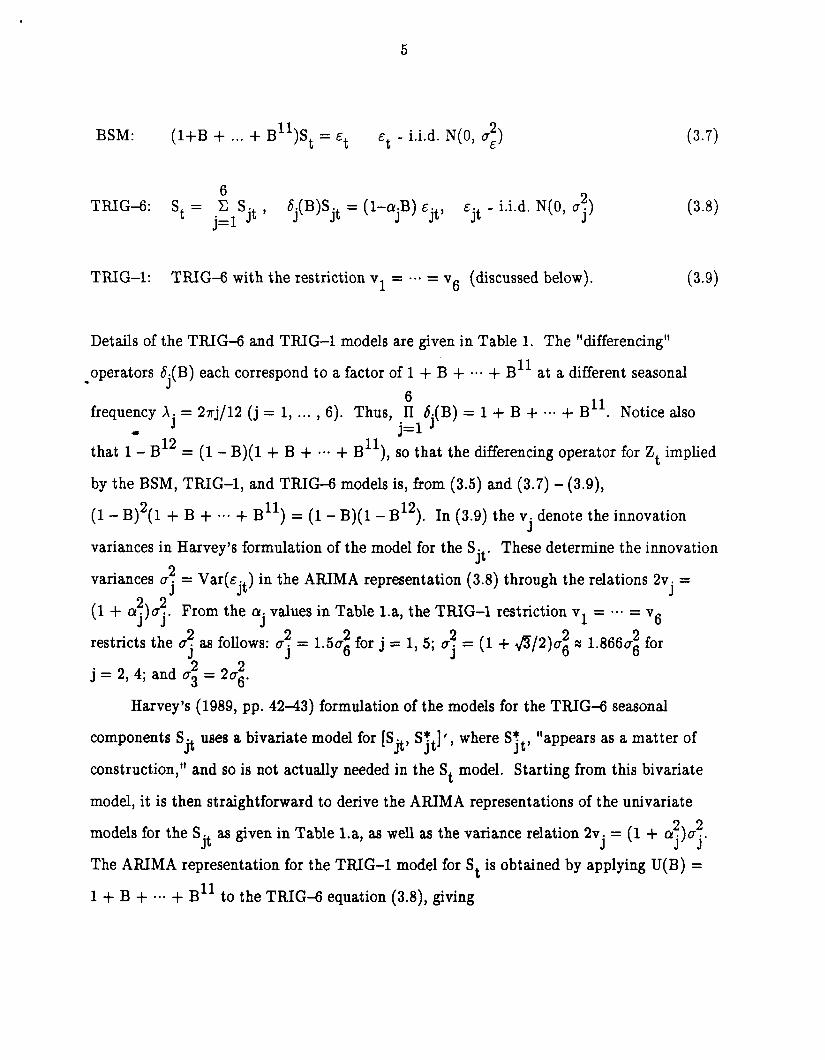
BSM: (l+B + . . . + B’l)S, = &t ct - i.i.d. N(0, 0:) (3.7)

TRIG-6: St= is. ) j = 1 Jt

6j(B)Sjt = (l-orjB) Ejt, &jt - i.i.d. N(0’ gi) (3.8)

TRIG-l: TRIG-6 with the restriction vl = a.. = v6 (discussed below). W)

Details of the TRIG-6 and TRIG-l models are given in Table 1. The “differencing”

. operators 6j(B) each correspond to a factor of 1 + B + ... + B1’ at a different seasonal

6 frequency Xj = 2rj/12 (j = 1, . . . , 6). Thus, II 6j(B) = 1 + B + *a* + B”. Notice also

that 1: B12

j=l

= (1 -B)(l + B + ... + Bll), so that the differencing operator for Zt implied

by the BSM, TRIG-l, and TRIG-6 models is, from (3.5) and (3.7) - (3.9),

(l- B)2(1 + B + ... + B’l) = (1 - B)(l - B12). In (3.9) the vj denote the innovation

variances in Harvey’s formulation of the model for the S. Jt ’

These determine the innovation

2 variances Q. =

(1 + *$f+J

Var(Ejt) in the ARIMA representation (3.8) through the relations 2vj =

From the ~j values in Table l.a, the TRIG-l restriction vl = ... = v6

restricts the g2 as follows: a? = 1.5~; for j = J J

1, 5; 0: = (1 + a/2)0; z 1.8660: for

j= 2, 4; and CT: = 2g;.

Harvey’s (1989, pp. 42-43) formulation of the models for the TRIG4 seasonal

components Sjt uses a bivariate model for [Sjt, STt]‘, where S5t, “appears as a matter of

construction,” and so is not actually needed in the St model. Starting from this bivariate

model, it is then straightforward to derive the ARIMA representations of the univariate

models for the S. as given in Table l.a, as well as the variance relation 2v. = (1 + c$$. Jt J

The ARIMA representation for the TRIG-l model for St is obtained by applying U(B) =

l+B+ .a. + B1’ to the TRIG-6 equation (3.8), giving

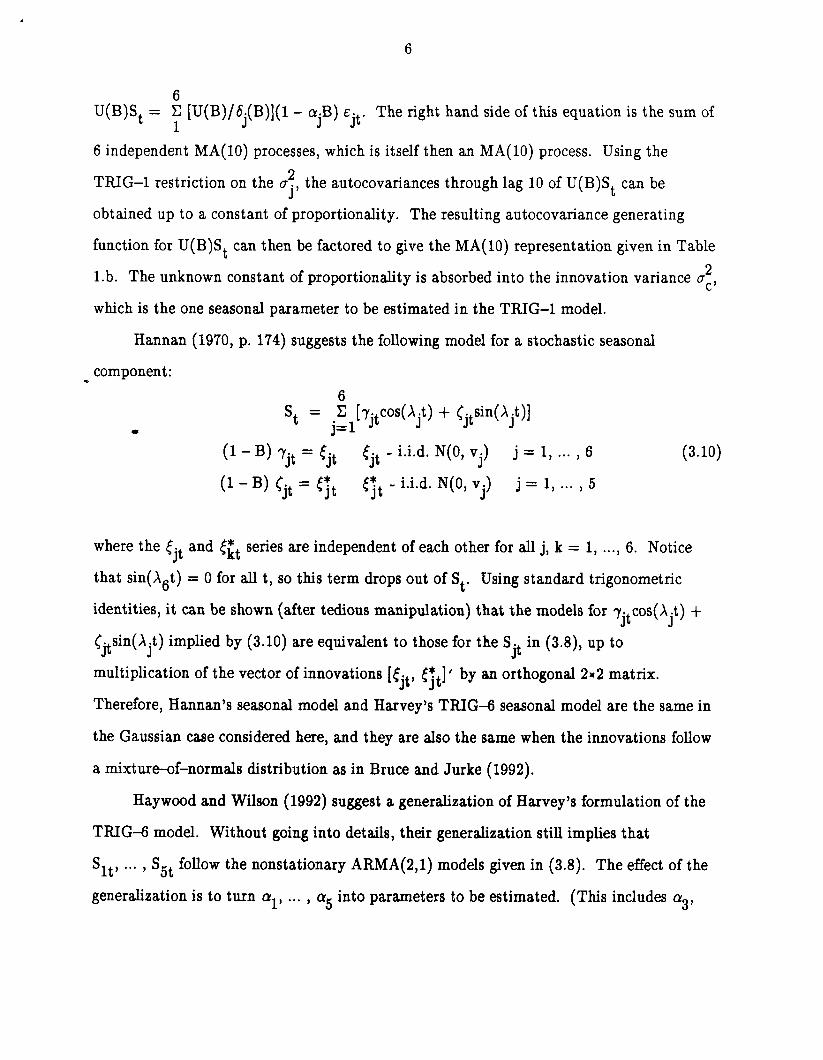
6

U(B)S, = i [U(B)/Gj(B)I(l - "jB) Ejt* The right hand side of this equation is the sum of

6 independent MA(lO) processes, which is itself then an MA(lO) process. Using the

TRIG-l restriction on the gf, the autocovariances through lag 10 of U(B)S, can be

obtained up to a constant of proportionality. The resulting autocovariance generating

function for U(B)S, can then be factored to give the MA(lO) representation given in Table

1.b. The unknown constant of proportionality is absorbed into the innovation variance c:,

which is the one seasonal parameter to be estimated in the TRIG-l model.

Hannan (1970, p. 174) suggests the following model for a stochastic seasonal

component: .

St = *

j~lL7jtCOS(Aj') + CjtsinCAjt)l

(1 -B) ~jt = ~jt Ijt - i.i.d. N(0, vj) j = 1, . . . , 6 (3.10)

(1 - B) Cjt = tTt tjt - i.i.d. N(0, vj) j = 1, . . . , 5

where the ~jt and [it series are independent of each other for all j, k = 1, . . . . 6. Notice

that sin( A6t) = 0 for all t, so this term drops out of St. Using standard trigonometric

identities, it can be shown (after tedious manipulation) that the models for Tjtcos(Xjt) +

<jtsin(Xjt) implied by (3.10) are equivalent to those for the Sjt in (3.8), up to

multiplication of the vector of innovations [[. <? Jt’ Jt

1’ by an orthogonal 2x2 matrix.

Therefore, Hannan’s seasonal model and Harvey’s TRIG-6 seasonal model are the same in

the Gaussian case considered here, and they are also the same when the innovations follow

a mixture-of-normals distribution as in Bruce and Jurke (1992).

Haywood and Wilson (1992) suggest a generalization of Harvey’s formulation of the

TRIG-6 model. Without going into details, their generalization still implies that

Q’ *** , Sgt follow the nonstationary ARMA(2,l) models given in (3.8). The effect of the

generalization is to turn al, . . . , o5 into parameters to be estimated. (This includes 03,

7

which is constrained to 0 in Harvey’s formulation. Also, note that the model for Sgt is

unchanged.) For the 40 time series used in this paper, however, this more general model

was found to fit uniformly worse (as measured by AIC) than the standard TRIG-6 model.

For this reason, the Haywood-Wilson model will not be considered further here.

The TRIG* model can also be written in an alternative “canonical” form, along the

lines that BP developed a canonical version of the BSM. Details are available from the

author on request. This canonical form provides an equivalent model for the observed

series Yt (at least for the Gaussian case), while transferring as much white noise as possible

from the individual seasonal components Sjt to the irregular It. This is in the spirit of the

-approach to seasonal decomposition developed by Burman (1980) and Hillmer and Tiao

(1982) for AROMA models. A canonical form of the TRIG-l model can also be developed

from tie TRIG-6 model under the restriction vl = ..a = v& BP found the canonical BSM

to be nearly identical to the original BSM, but such is not the case for the TRIG-6 and

TRIG-l models. Thus, use of the canonical form has potential consequences for seasonal

adjustment, although for the one example I have examined so far, seasonal adjustment

results from the original and canonical TRIG-6 models have been essentially the same.

BP review some alternative ARIMA component models that have been proposed.

One such model involves augmenting the BSM with a fourth component to account for

possible cyclical behavior (Harvey 1985). BP encountered severe numerical problems in

trying to fit such models, and so did not report results for them. Since that writing I have

been successful in fitting these models with the fourth component following an AR(2)

model. The augmenting of the BSM with this fourth component did nothing to improve its

performance relative to the ARIMA models for the series considered in BP. In fact, for

about 3/4 of the series the innovation variance of the fourth component was estimated to

be essentially zero, indicating that the fourth component was not really present anyway.

(Harvey (1985) also found little evidence of cyclical components in the 5 U.S. postwar

8

economic time series he analyzed, though he found more evidence of cycles in the prewar

data.) Given these results, models with a fourth cycle component will not be considered in

this paper.

4. Data

The ARIMA and ARIMA component models will be compared using a set of 40

monthly time series that are broadly representative of the time series that are seasonally

adjusted by the Census Bureau. 27 of these series were also used in BP, although the time

frames of the actual data used here are different. The time frames used here are those of

- Kramer, Bell, and Koreisha (1993), and yield n = 200 observations for each series.

Space constraints prevent my giving further information on the data here. Details on

the dlta series are available on request.

5. Emnirical Results

The ARIMA and the ARIMA component models (BSM, TRIG-l, and TRIG-6) were

fit to the 40 time series by maximum likelihood using the REGCMPNT computer program

developed by the time series staff of the Census Bureau. The likelihood function is defined

as the joint density of the differenced data: (1 - B)(l - B12)Yt for t = 14, . . . , n.

REGCMPNT evaluates the likelihood using the Kalman filter initialized as described in

Bell and Hillmer (1991). The fit of the various models will be compared here in terms of

various commonly used model selection criteria. These are AIC (Akaike 1973); AIC,, a

bias corrected version of AIC (Hurvich and Tsai 1989); HQ (Hannan and Quinn 1979); and

BIC (Schwarz 1978). If t denotes the value of the log-likelihood evaluated at the

maximum likelihood parameter estimates for a given model, and m is the number of

parameters in the model, then the criteria are defined as follows, using n - 13 (= 187) as

the number of observations of the differenced data.

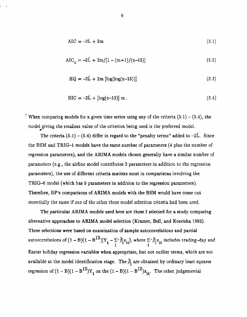
AIC = -2l!, + 2m

AIC, = -2L + 2m/[l- (m+l)/(n-13)]

HQ = -2L + 2m [log(log(n-13))]

BIC = -2i + [log(n-13)] m .

(5.1)

(5.2)

(5.3)

(5.4)

* When comparing models for a given time series using any of the criteria (5.1) - (5.4), the

model giving the smallest value of the criterion being used is the preferred model. *

The criteria (5.1) - (5.4) differ in regard to the “penalty terms” added to -2i. Since

the BSM and TRIG-l models have the same number of parameters (4 plus the number of

regression parameters), and the ARIMA models chosen generally have a similar number of

parameters (e.g., the airline model contributes 3 parameters in addition to the regression

parameters), the use of different criteria matters most in comparisons involving the

TRIG-6 model (which has 9 parameters in addition to the regression parameters).

Therefore, BP’s comparisons of ARIMA models with the BSM would have come out

essentially the same if one of the other three model selection criteria had been used.

The particular ARIMA models used here are those I selected for a study comparing

alternative approaches to ARIMA model selection (Kramer, Bell, and Koreisha 1993).

These selections were based on examination of sample autocorrelations and partial

autocorrelations of (1 - B)(l - B12)[Yt - C’~ixit], where B/B includes trading-day and i i

ixit

Easter holiday regression variables when appropriate, but not outlier terms, which are not

available at the model identification stage. The 4 are obtained by ordinary least squares

regression of (1 - B)( 1 - B12)Yt on the (1 - B)( 1 - B12)xit. The other judgemental

10

ARIMA model selections reported in Kramer, Bell, and Koreisha (1993) produced, on

average, comparable AIC values. Therefore, the empirical results presented here might be

regarded as representative in regard to the performance of ARIMA models.

Table 2.a presents a summary of the AIC differences over the 40 time series for each

pair of models considered. The first 3 lines of the table show the results comparing the

ARIMA and ARIMA component models. Positive values favor the ARIMA models;

negative values favor the ARIMA component models. AIC expresses a strong preference

overall for the ARIMA models: only a few of the AIC differences in these comparisons are

negative, and those that are negative are almost all small to moderate in magnitude (< 8),

* while most of the AIC differences are positive, and many of these positive differences are

large f> 8).

The middle 3 lines of Table 2.a present comparisons of the ARIMA component

models with each other. The median AIC differences are small for the two comparisons

involving the BSM, and there is a median AIC difference of 3.2 slightly favoring the

TRIG-l over the TRIG-6 model. However, the presence of negative values large in

magnitude in all of these comparisons shows that sometimes the BSM fits quite poorly in

comparison with the TRIG-l and TRIG-6 models, as can the TRIG-l in comparison to

the TRIG-6. Thus, the TRIG-l and TRIG-6 models appear definitely favored over the

BSM, while the choice between the TRIG-l and TRIG-6 models is less clear. In general,

having the 6 different seasonal variance parameters of the TRIG4 model sometimes is

unnecessary, but occasionally this achieves a major improvement in model fit over the

TRIG-l model (as measured by AIC).

Bruce and Jurke (1992) report AIC’s for the non-Gaussian versions of the BSM,

TRIG-l, and TRIG-6 models as fitted by the MING program to 29 of the 40 series

considered here. Their results would not be expected to be the same as those reported here

because of the non-Gaussian fitting, and because Bruce and Jurke used different time

11

frames of the series. Still, the AIC relationships for their non-Gaussian BSM, TRIG-l,

and TRIG-6 models are similar to those found here for most of the series they consider,

although there are some notable exceptions.

The final four lines in Table 2.a compare the fit of the four models already considered

(ARIMA, BSM, TRIG-l, and TRIGd) with the airline model (3.3). As in BP, these

comparisons are presented to check the possibility of selection bias favoring the ARIMA

model. (The particular ARIMA models chosen were not chosen to minimize AIC, but the

usual identification procedures could have a similar effect.) The first of these lines

compares the airline model with the selected ARIMA models. The median AIC difference

* is 0; in fact, 14 of the 40 selected ARIMA models were the airline model. Aside from this,

the results are as would be expected: almost all the nonzero AIC differences are negative,

indicating that selection of a particular ARIMA model for each series improved model fit

as measured by AIC. There are a few exceptions where the airline model comes out

slightly favored, but what is more important is the occurrence of some negative AIC

differences that are large in magnitude, indicating that for a few series the airline model

provided poor fits. Two of these series are responsible for the large-in-magnitude negative

AIC differences in the final three lines of Table 2.a, indicating a strong preference for the

ARIMA component models over the airline model for these two series. Apart from these

two series, the results are not very different from the results of the ARIMA and ARIMA

component model comparisons. On balance, AIC expresses a strong preference for the

airline model over the ARIMA component models.

As expected, the effects of using one of the model comparison statistics other than

AIC is very slight for comparisons that do not involve the TRIG4 model. The effect of

using the bias corrected AIC (AIC,) is to make the TRIG-6 model look slightly worse

relative to the other models. The effect of using HQ or BIC, however, is to make the

TRIG-6 model look dramatically worse relative to the other models. This is seen by

12

comparing the results in Tables 2.a and 2.b that summarize AIC and HQ differences

involving the TRIG-6 model. The effects in going to the BIC are even more dramatic.

This effect is, of course, due to the penalty terms. The increases in the HQ and BIC

penalty terms for the TRIG-6 model versus the BSM or TRIG-l models are:

HQ : penalty increase = 2{log[log(187)]}(9 - 4) = 16.5

BIC : penalty increase = [log(187)](9 - 4) = 26.2 a

- 6. Discussion

The results presented here provide further evidence to that in BP and Findley (1990)

of the*superiority of ARIMA models to the BSM. Actually, for the 27 of the 40 series used

here that were used in BP, albeit over different time frames, the ARIMA-BSM

comparisons reported here are best interpreted as confirming the findings of BP with a

more controlled study of almost the same data. What is both new and important in this

paper is that the results also show marked superiority of the ARIMA models (and the

airline model) over the TRIG-l and TRIG-6 models for the series considered. Thus, in

general, it appears that all the ARIMA component (structural) models tend to provide a

poor fit to the sort of time series seasonally adjusted by the Census Bureau.

BP noted that the BSM is much more difficult to fit than ARIMA models. In

performing this study I have further found the TRIG-6 model to be even more difficult to

fit than the BSM. The TRIG-l model is also more difficult to fit than the BSM, though

not so difficult to fit as the TRIG-6 model. One problem that arises in fitting all the

ARIMA component models occurs when the maximum likelihood estimate (MLE) of 77 in

(3.5) is 1, something that occurs fairly frequently. Another problem that surfaces with the

TRIG-6 model occurs when the MLE of one or more of the 6 seasonal variance parameters

13

is essentially 0. This is also not an infrequent occurrence. The need to estimate

parameters at such boundary values poses rather difficult numerical problems for nonlinear

optimization algorithms. The same sort of difficulty arises with the ARIMA model (3.2) .

when g12 = 1. This occurs occasionally, but much less frequently than the analogous

problems for the ARIMA component models. It also appears that, for all the ARIMA

component models, the likelihood is rather flat in certain directions in the parameter space.

Given this, I find the oft-claimed advantages of simplicity and interpretability for ARIMA

component models difficult to accept.

. REFERENCES

Akd;ke, H. (1973) “Information Theory and an Extension of the Likelihood Principle,” in the 2nd International Svmposium on Information Theory, eds. B. N. Petrov and F. Czaki, Budapest: Akademia Kiado, 267-287.

Bell, W. R. (1983 , Proceedings o I

“A Computer Program for Detecting Outliers in Time Series,” the American Statistical Association, Business and Economic

Statistics Section, 634-639.

(1987 “A Note on Overdifferencing and the Equivalence of Seasonal Time Series MO d els With Monthly Means and Models With (0,1,1)12 Seasonal Parts When 8 = 1,” Journal of Business and Economic Statistics, 5, 383-387.

Bell, W. R. and Hillmer, S. C. (1983) “Modeling Time Series with Calendar Variation,” Journal of the American Statistical Association, 78, 526-534.

(1991) “Initializing the Kalman Filter for Nonstationary Time Series Models,” Journal of Time Series Analysis, 12, 283-300.

Bell, W. R. and M. G. Pugh (1990 Time Series Components , I’ An a(

“Alternative Approaches to the Analysis of vsis of Data in Time, Proceedings of the 1989

International SvnmDosium, A.C. Singh and P. Whitridge eds., Statistics Canada, 105-116.

Box, G.E.P. and Jenkins, G. M. (1970) Time Series Analysis: Forecasting and Control, San Francisco: Holden Day.

Bruce, A. G. and Jurke, S. R. (1992) “Non-Gaussian Seasonal Adjustment: X-12 ARIMA Versus Robust Structural Models,” Research Report No. 92/14, Statistical Research Division, Bureau of the Census, Washington, D.C.

14

Burman, J. P. (1980) “Seasonal Adjustment by Signal Extraction,” Journal of the Royal Statistical Society, A, 143, 321-337.

Chang, I., Tiao, G. C., and Chen, C. (1988) “Estimation of Time Series Parameters in the Presence of Outliers,” Technometrics, 30, 193-204.

Findley D. F. (1990 90/11, Statistic a

“Making Difficult Model Comparisons,” Research Report No. Research Division, Bureau of the Census, Washington, D.C.

Garcia-Ferrer, A. and de1 Hoyo, J. (1992) “On Trend Extraction Models: Interpretation, Empirical Evidence, and Forecasting Performance” (with discussion), Journal of Forecasting, 11, 645-674.

Hannan, E. J. (1970) Multime Time Series, New York: John Wiley.

Hannan, E. J. and Quinn, B. G. (1979) “The Determination of the Order of an Autoregression,” Journal of the Royal Statistical Society, B, 41, 190-195.

w Harvey, A. C. (1985), “Trends and Cycles in Macroeconomic Time Series,” Journal of Business and Economic Statistics, 3, 216-227.

(1989) Forecasting. Structural Time Series Models and the Kalman Filter, Cambridge, U. K.: Cambridge University Press.

Harvey, A. C. and Todd, P. H. J. Structural and Box-Jenkins 6

1983), MO els:

“Forecasting Economic Time Series With A Case Study,” (with discussion), Journal

of Business and Economic Statistics, 1, 299-315.

Haywood, J. and Wilson, G. Tunnicliffe (1992) “On the Choice of State Space Representation for Trigonometric Components of Seasonal Time Series,” unpublished manuscript, Mathematics department, Lancaster University, U.K.

Hillmer, S. C., and Tiao, G. C. (1982) “An ARIMA-Model-Based Approach to Seasonal Adjustment,” 63-70.

Journal of the American Statistical Association, 77,

Hurvich, C. M. and Tsai, C. (1989) “Regression and Time Series Model Selection in Small Samples,” Biometrika, 76, 297-307.

Kramer, M., Bell, W. R., and Koreisha, S. (1993) “A Comparison of Automatic and Judgement al ARIMA Model Selection, I’ paper presented at the 1993 meeting of the American Statistical Association, San Francisco, CA.

Schwarz, G. (1978) “Estimating the Dimension of a Model,” Annals of Statistics, 6, 461464.

15

Table 1

a. ARlMA Representations for the Individual TRIG-6 !Zeasonal Components

6 TRIG-6 Seasonal Model: St = C S.

1 Jt

[l - 2 cos(Xj)B + B2] Sjt = (1 - “jB) &jt j = 1, *** 9 5 (‘j = 2r.i/12)

(l + B, ‘gt = &(jt Ejt - i.i.d. N(0, CT!) j = 1, . . . , 6

“Differencing” MA Operator Operator

l-&B+B2 1 - (@/3)B 1-B+B2 1 - (2-,@B

1 +B2 1

l+B+B2 1+ (24)B

1+ p+ +BB2 1 + ywP

b. ARIMA Representation of the TRIG-1 Seasonal Component

(1 + B + *** + B”) St = (1 - alB - ... - ctlOB1’) ct ct - i.i.d. N(0, CT:)

a1 = -.737378 9 = -.627978 ct3 = -.430368 cr4 = -.360770

a5 = -.219736 a6 = -.180929 (u7 = -.088488 a8 = -.071423

cl9 = -.020306 “10 = -.016083

16

Table 2

a. AIC Comparisons

(-oo,-30 P,--2)

k-2,21 BSM-ARIMA 0 0 0 1

TRIGl-ARIMA 0 0 1: TRIGG-ARIMA 0 i 2 : 2

TRIGl-BSM TRIGG-BSM Fi x i: x

23 4

TRIGG-TRIG1 0 2 4 6 6

WARIMA-Airline 1 3 2 24* BSM-Airline 1 1 1 x 10

TRIGl-Airline 1 1 14 TRIGfi-Airline 1 : 1 s 2

PA

12 14 13

2 12 19

3 11 15 13

b. Hannan-Quinn (HQ) Comparisons

(-q-30 -3O,-16

I 1 -16,-8) P,-2)

[-WI cul

BSM-ARIMA 0 i i

2 4 15 TRIGl-AR.IMA 0 TRIGG-ARIMA 0 0 0 ii i

19 2

TRIGl-BSM 0 5 23 2 TRIGG-BSM TRIGG-TRIG1

ii ii

: 47 1 3 i 8’

ARIMA-Airline 1 2 11 21* 4 BSM-Airline ;

TRIGl-Airline : : 0 : : 8; TRIGG-Airline 0 1 1 1 2 2

w31 (16,301

(3OF)

7

2: :

2

2 i

ii i i 3 0 0

: 6 0 0 2

5 2 17 1 i!i

@,W (16,301

(3Ow)

8 2 10 : 1 15 19 1

0

ii x 8 0 0

ii !:

0 2

4 3 1 15 17 1

* 14 of the AIC and HQ differences are exactly 0 because 14 of the selected ARTMA models are the airline model.