Turk J Elec Eng & Comp Sci

(2017) 25: 4211 – 4222

c⃝ TUBITAK

doi:10.3906/elk-1612-203

Turkish Journal of Electrical Engineering & Computer Sciences

http :// journa l s . tub i tak .gov . t r/e lektr ik/

Research Article

Time-jerk optimal trajectory planning of a 7-DOF redundant robot

Shaotian LU, Jingdong ZHAO∗, Li JIANG, Hong LIUState Key Laboratory of Robotics and System, Harbin Institute of Technology, Harbin, P.R. China

Received: 16.12.2016 • Accepted/Published Online: 18.05.2017 • Final Version: 05.10.2017

Abstract: In order to improve the efficiency and smoothness of a robot and reduce its vibration, an algorithm called the

augmented Lagrange constrained particle swarm optimization (ALCPSO), which combines constrained particle swarm

optimization with the augmented Lagrange multiplier method to realize time-jerk (defined as the derivative of the

acceleration) optimal trajectory planning is proposed. Kinematic constraints such as joint velocities, accelerations, jerks,

and traveling time are considered. The ALCPSO algorithm is used to avoid local optimization because a new particle

swarm is newly produced at each initial time process. Additionally, the best value obtained from the former generation

is saved and delivered to the next generation during the iterative search for process. Thus, the final best value can be

found more easily and more quickly. Finally, the proposed algorithm is tested on the 7-DOF robot that is presented in

this paper. The simulation results indicate that the algorithm is effective and feasible. Hence, the algorithm presents a

solution for the time-jerk optimal trajectory planning problem of a robot subject to nonlinear constraints.

Key words: Particle swarm optimization, jerk, cubic splines, trajectory planning, redundant robot

1. Introduction

Optimal trajectory planning is an optimal control problem in robots. The planning task includes planning an

optimal smooth trajectory that meets the boundary conditions based on the given path points [1]. Reasonable

trajectory planning can improve the working efficiency of the robot and reduce its vibration and trajectory

tracking errors.

Minimum-time trajectory planning was first proposed in the literature, and the purpose involved maxi-

mizing the traveling speed to minimize the total traveling time of the robot. Minimum-jerk trajectory planning

has several advantages. It reduces stress on the actuators and the structure of the robot. It also reduces

vibration when the robot is in motion and can improve trajectory tracking accuracy.

Recently, various researchers have focused on the time-jerk optimal trajectory planning problem in order

to improve the efficiency and smoothness of the robot and reduce its vibration. This problem combines minimum-

time with the minimum-jerk trajectory planning problem. Examples of this type of trajectory planning were

discussed in [2–6]. After summarizing previous research on optimal trajectories planning, the main research

procedure in this paper involves the following steps: first, a mathematics objective function is applied to

express the optimal problem. Second, optimal methods are adopted based on problem properties to solve the

mathematical objective function. Finally, optimal results are compared and relational results are selected based

on the requirements. Most engineering problems belong to nonlinear constraint programming problems and

thus constraint optimal methods are commonly used to solve these problems.

∗Correspondence: stlu2008@163.com

4211

LU et al./Turk J Elec Eng & Comp Sci

Currently, interpolated functions in joint space are mainly utilized by researchers and include cubic

spline and fifth-order B-spline. The main optimal methods include the genetic algorithm, PSO, and sequential

quadratic programming (SQP) algorithms. Extant research on time-jerk optimal trajectory planning reveals

three problems. First, research in this area is still relatively limited and thus it is necessary to perform an in-

depth study. Second, many studied objects are simple, and the research done on redundant robots is especially

rare. Third, the penalty function method is typically used to solve the optimal trajectory planning objective

function. However, sometimes the optimal solution can only be obtained when the penalty factor becomes

infinitely large (for the exterior penalty function method) or infinitely small (for the interior penalty function

method) values due to the defects of the penalty function method. Thus, the iterative search for velocity is slow.

Additionally, if the initial value of the penalty factor is improperly used, the penalty function may go into an

abnormal state that makes optimal calculation difficult. Therefore, numerous tests are required to determine a

practical initial penalty factor. Previous studies have presented some optimal algorithms. However, it is difficult

to easily and quickly make a nonlinear constrained problem converge to an optimal solution.

In this paper, a new algorithm for time-jerk optimal trajectory planning is proposed to improve the

efficiency and reduce the vibration of a robot. The new algorithm is called the augmented Lagrange constrained

particle swarm optimization (ALCPSO) algorithm, and it applies the constriction factor method originating from

the basic PSO algorithm and combines it with the augmented Lagrange multiplier (ALM) method. However,

in contrast to some previous studies, a new particle swarm is newly produced each time in the initial procedure

so that it avoids local optimization. Additionally, the best value obtained from the former generation is saved

and delivered to the next generation during the iterative search for process. Consequently, the ultimate best

value can be acquired more easily and more quickly, even for finite penalty factors.

The paper is organized as follows: Section 2 presents the 7-DOF redundant robot that will be used

and studied in this paper. The time-jerk optimal trajectory planning problem is described in Section 3. The

application of the ALCPSO method that solves the nonlinear constrained optimization problem is described in

Section 4. Section 5 shows the simulation results of the ALCPSO algorithm and Section 6 is the conclusion.

2. The 7-DOF redundant robot and its inverse kinematics

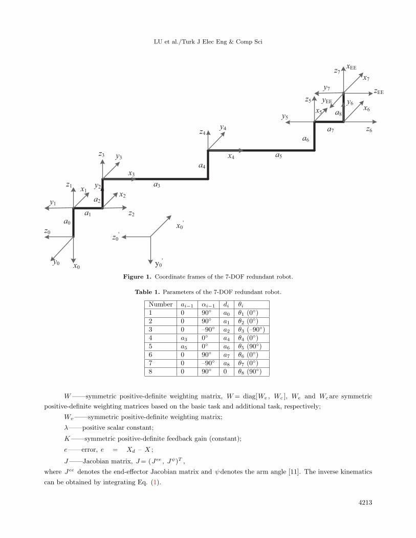
In this paper, the configuration of the introduced 7-DOF redundant robot resembles that of the Space Station

Remote Manipulator System. The robot is composed of seven modular joints, and its coordinate frames are

shown in Figure 1. The corresponding parameters are shown in Table 1. The transformation matrix of the 7-

DOF robot can be gained by each known transformation of the D-H matrix i−1iT [7,8]. The coordinate frames

F0′ (x0

′ y ′0 z0

′) are added to conveniently compute the transformation matrix. First, the transformation

matrix 00′T from F0 to F0′ is obtained, and then the following transformation matrices can be derived based

on the transformation of matrix 00′T .

It is necessary to obtain the inverse kinematics of the robot prior to optimizing its trajectory. In this

paper, the configuration control scheme is used to solve the inverse kinematics of the 7-DOF redundant robot

because this method can guarantee unique inverse kinematics and enable the robot to carry out cyclic motion,

which is important for repetitive operations [9,10]. Additionally, this method can be computed very quickly,

which is especially favorable for real-time control of the redundant robot. The damped-least-squares (DLS)

formulation of the configuration control is expressed as:

q =W−1v JT [JW−1

v JT + λ2W−1]−1(Xd +Ke), (1)

where:

4212

LU et al./Turk J Elec Eng & Comp Sci

x1z1

y1

x0y0

z0

a0

a1

a2

a3

a4

a5

a6

a7

a8

x2

x3

x4

x5x6

x7

xEE

yEE

zEE

y2

y3

y4

y5

y6

y7

z2

z3

z4

z5

z6

z7

x0'

y0'

z0'

Figure 1. Coordinate frames of the 7-DOF redundant robot.

Table 1. Parameters of the 7-DOF redundant robot.

Number ai−1 αi−1 di θi1 0 90◦ a0 θ1 (0◦)2 0 90◦ a1 θ2 (0◦)3 0 –90◦ a2 θ3 (–90◦)4 a3 0◦ a4 θ4 (0◦)5 a5 0◦ a6 θ5 (90◦)6 0 90◦ a7 θ6 (0◦)7 0 –90◦ a8 θ7 (0◦)8 0 90◦ 0 θ8 (90◦)

W——symmetric positive-definite weighting matrix, W = diag[We , Wc ], We and Wcare symmetric

positive-definite weighting matrices based on the basic task and additional task, respectively;

Wv——symmetric positive-definite weighting matrix;

λ——positive scalar constant;

K——symmetric positive-definite feedback gain (constant);

e——error, e = Xd – X ;

J——Jacobian matrix, J= (Jee , Jψ)T ,

where Jee denotes the end-effector Jacobian matrix and ψdenotes the arm angle [11]. The inverse kinematics

can be obtained by integrating Eq. (1).

4213

LU et al./Turk J Elec Eng & Comp Sci

3. The time-jerk optimal trajectory planning description

The cubic spline is used very frequently in trajectory planning because it has many advantages. In contrast to

higher order polynomials, it can overcome excessive oscillations and overshoot, and the generated trajectories

have continuous acceleration values. In this paper, the cubic spline in [2,3] is used to plan the trajectory. The

effect of trajectory planning mainly relies on the optimal objective function. In this paper, the time-jerk optimal

objective function is that of [4] and is described as follows:

min f(h) = KTNn−1∑i=1

hi + αKJ

N∑i=1

n−1∑i−1

[(Qj,i+1−Qj,i)

2

hi

]s.t.

max{∣∣∣Qj,i(ti)∣∣∣ , ∣∣∣Qj,i(ti∗)∣∣∣ , ∣∣∣Qj,i(ti+1)

∣∣∣} − Vjm ≤ 0

max{∣∣∣Qj,1(t1)∣∣∣ , ∣∣∣Qj,2(t2)∣∣∣ , · · · , ∣∣∣Qj,n(tn)∣∣∣} −Ajm ≤ 0

max∣∣∣ Qj,i(ti+1)−Qj,i(ti)

hi

∣∣∣− Jjm ≤ 0

n−1∑i=1

hi − Tm ≤ 0

j = 1, . . . , N∀i = 1, . . . , n− 1 (2)

In the optimization problem in Eq. (2), KT +KJ= 1. Table 2 describes the meaning of the symbols in Eq.

(2). The traveling time and the function of jerk perhaps have a large difference in quantity; thus, the elastic

coefficient is introduced to balance the effect of traveling time and the function of jerk. In practice, the total

traveling time and jerk function can reach an optimum level to some degree by adjusting KT and KJ . By

solving Eq. (2) to gain the optimal time intervals, the time-jerk optimal trajectory under constraints can be

obtained after adopting the cubic spline to plan trajectory.

Table 2. Meaning of the symbols.

Name Meaning Name Meaning

N Number of robot joints Qj(t) Velocity of the jth joint

KT Time weighting coefficient Qj(t) Acceleration of the jth jointhi Time interval between two plan points Qj(t) Jerk of the jth jointAjm Acceleration limit for the jth joint (symmetrical) Vjm Velocity limit for the jth joint (symmetrical)Tm Traveling time limit KJ Jerk weighting coefficientn Number of via points Jjm Jerk limit for the jth joint (symmetrical)

4. Solving the time-jerk optimal trajectory planning problem

The CPSO and ALM methods possess their own advantages; therefore, these two methods are adopted to solve

the time-jerk optimal trajectory planning problem.

4.1. Constrained particle swarm optimization

Generally, PSO includes the following advantages: it is simpler and easier to use in practice when compared to

some other optimal algorithms; it is more compatible and robust than some other classical optimal methods;

and it possesses a global convergence ability and thus can be used to solve nonlinear optimization problems.

4214

LU et al./Turk J Elec Eng & Comp Sci

In [12,13], the constriction factor χ was introduced to ensure the convergence of the PSO as follows:

χ =2∣∣∣2− φ−√φ2 − 4φ

∣∣∣ , φ = c1 + c2, φ > 4 (3)

In PSO, the particle velocity and position are updated as follows:

vij(k + 1) = χ[vij(k) + c1r1[pij(k)− xij(k)] + c2r2[gj − xij(k)]]

xij(k + 1) = xij(k) + vij(k + 1)1 ≤ i ≤ n∀1 ≤ j ≤ Nd,max (4)

In Eq. (3), researchers usually set c1 = c2 = 2.05, and φ is normally set to 4.1 so that χ = 0.729. Hence,

the PSO can be called the constrained particle swarm optimization (CPSO) algorithm, and it can achieve an

effective balance between the global search and the local search.

4.2. Augmented Lagrange multiplier (ALM) method

The ALM method resembles the penalty function method. However, the ALM method does not require many

tests to determine a practical initial penalty factor. Additionally, the penalty factor of the ALM method does

not need to tend to infinity [14–16], and it surpasses the penalty function method in numerical stability and

calculated efficiency.

For the general inequality constrained problem, the optimal model can be written as:

min f(X)

s.t.gj(X) ≤ 0j = 1, . . . ,m (5)

Its ALM method can be described as follows:

L(X,λ, r) = f(X) +m∑j=1

[λjφj + rjφ2j ], (6)

where X= (x1 , . . . , xn) denotes the independent variable, f(X) denotes the objective function, gj(X) ≤ 0 (j

= 1, ... , m) for the j th inequality constraints, λj denotes the j th Lagrange multiplier, and rj denotes the

j th penalty factor. φj is described as follows:

φj = max(gj(x),−λj2rj

) j = 1, . . . ,m (7)

In the process of reaching a solution, the iterative updated formula of the Lagrange multiplier is expressed as

follows:λv+1j = λvj + 2rjφj , (8)

where ν denotes the ν th update time of the Lagrange multiplier. The iterative updated formula of the penalty

factor is described as follows:

rv+1i =

2rvj |gj(Xv)| >

∣∣gj(Xv−1)∣∣ ∧ |gj(Xv)| > εg

rvj2 |gj(Xv)| ≤ εg

rvj else

, (9)

where εg denotes constraint error accuracy.

4215

LU et al./Turk J Elec Eng & Comp Sci

When ν= 1, the termination criteria are expressed as follows:

c = max{max[0, gj(Xv)] ≤ ε j = 1, · · · ,m ∀i = 1, · · · , vmax} (10)

When ν = 2,. . . ,vmax , the iteration termination criteria are defined as follows:

|L(X,λ, r)− f(X)| ∧ c ≤ ε, (11)

where εdenotes the convergence accuracy and vmax denotes the update maximal times.

4.3. Augmented Lagrange constrained particle swarm optimization (ALCPSO) algorithm

Both the CPSO and ALM methods possess their own unique advantages. As a result, the CPSO method is

combined with the ALM to benefit from the advantages of each method to offer a new solution for the nonlinear

constrained optimal problem. Time-jerk optimal trajectory planning belongs to this category of problem. The

key issue involves presenting a reasonable and practical algorithm.

In this paper, the ALCPSO algorithm is proposed, and it involves a combination of the ALM and the

CPSO methods. The main idea of this algorithm is expressed as follows: First, the ALM method is utilized

to transform the constrained problem (Eq. (5)) into the unconstrained problem (Eq. (6)). Second, random

data are then adopted to produce a group of particles as an initial value. Third, a determination is made as

to whether or not the termination criteria (Eq. (10)) are satisfied, and the best solution is obtained if the

termination criteria are satisfied. Otherwise, the obtained best solution is saved. A new unconstrained problem

(Eq. (6)) is then presented, and we need to apply the random data to produce a new group of particles; the

CPSO algorithm is then adopted to update the particle velocities and positions of the particles and to determine

whether or not the termination criteria (Eq. (11)) are satisfied. We then need to apply Eqs. (8) and (9) to

update the Lagrange multiplier and the penalty factor during the iterative search for process. Finally, the global

best solution x∗ of the original constrained problem (Eq. (5)) can be obtained after repeated iterations.

In this algorithm, a new particle swarm is freshly produced in each initial process in order to avoid

local optimization. The ultimate best solution is obtained more easily and quickly because the best solution

acquired from the former generation is saved and delivered to the next generation during the iterative search

for process. Figure 2 shows the flowchart for adopting the ALCPSO algorithm to realize time-jerk optimal

trajectory planning. The flowchart of the ALCPSO algorithm is shown in the imaginary line frame.

4.4. Time-jerk optimal trajectory planning simulation of the 7-DOF redundant robot

It is necessary to obtain the inverse kinematics of the 7-DOF robot prior to executing optimal trajectory

planning. In this paper, the DLS approach is used as described in Section 2 to solve the inverse kinematics of

the 7-DOF robot. The values are set as follows: We = diag[1,1,1,1,1,1], Wc = 1, Wv= diag[1,1,1,1,1,1,1], K

= diag[1,1,1,1,1,1,1], and λ= 1, Xd = (0,0,0,0,0,0,0)T . In order to verify the effectiveness and practicality of

the proposed ALCPSO method, this method is utilized to implement time-jerk optimal trajectory planning of

the robot. The program is compiled in MATLAB R2014.

The geometric parameters of the 7-DOF robot are set as follows: a0 = 716.1 mm, a1 = 430 mm, a2

= 430 mm, a3 = 2080 mm, a4 = 387 mm, a5 = 2080 mm, a6 = 430 mm, a7 = 430 mm, and a8 = 716.1

mm. The robot will become singular if the joint angles defined in Table 1 are directly applied. In order to

prevent this, the initial joint angles are defined as follows: θ1 = 0◦ , θ2 = 0◦ , θ3 = –90◦ , θ4 = 60◦ , θ5 =

4216

LU et al./Turk J Elec Eng & Comp Sci

Figure 2. Flowchart of adoption of the ALCPSO algorithm for time-jerk optimal trajectory planning.

90◦ , θ6 = 0◦ , and θ7 = 0◦ . The tested mission is tracking a circle. The initial position of the end-effector

corresponds to –2679.2, –2173.7, and –3765.0 mm based on the coordinate frames F0 (x0y0 z0). The radius R

and the center of the track circle correspond to 1000 mm and –2679.2, –2173.7, and –2765.0 mm, respectively.

In this paper, in order to describe the trajectory plan points in the circle that the robot tracked, the trajectory

plan points are inferred from the planned circular central angle. The planned circular central angle is divided

into uniform acceleration, uniform velocity, and uniform deceleration with a total of three segments along the

counter-clockwise rotation. The robot, at an angular acceleration value of 120/(1/80 × n)2 ◦ /s2 (n represents

the number of planned via points), starts to accelerate from the initial position. When the robot along the

circle moves 60◦ , it completes the uniform acceleration segment, enters the uniform segment, and moves 240◦ ;

ultimately, the robot, accelerating at 120/(1/80 ×n)2 ◦ /s2 , enters the uniform deceleration section and returns

4217

LU et al./Turk J Elec Eng & Comp Sci

to the initial point, thereby completing the complete motion. In this paper, we set n= 8. Table 3 lists the values

of the plan points of the trajectory planning. As shown in Table 3, the 1-point coincides with the 9-point when

the robot completes a cyclic motion. Thus, there are 9 plan points and 8 via points. The kinematic constraints

of the joints are as follows: Vjm = 3 deg/s, Ajm = 3 deg/s2 , and Jjm = 5 deg/s3 (j = 1, . . . , N).

Table 3. Input data for trajectory planning.

JointPlan points (degrees)1 2 3 4 5 6 7 8 9

1 0

Virtual

–32.66 –37.74 –15.44 4.21 20.26

Virtual

–0.142 0 0.00 0.00 0.00 0.00 0.00 0.003 –90 –79.19 –79.02 –77.37 –79.99 –95.51 –89.784 60 88.73 116.13 112.24 81.75 55.89 58.955 90 91.92 84.66 75.24 79.18 87.44 95.526 0 0.00 0.00 0.00 0.00 0.00 0.007 0 –8.79 –24.03 –34.67 –25.15 –8.08 –4.56

Additionally, some other values are set as follows: traveling time constraint of the robot t = 150 s; initial

penalty factor r0 = (1000, . . . , 1000); initial Langrage multiplier λ0 = (0, . . . ,0); constrained error accuracy

εg = 0.0001; convergent accuracy ε= 0.0001; maximal update times of the penalty factor and the Lagrange

multiplier vmax = 100; swarm particle number Nd,max = 40; maximal iterative times of the CPSO kmax =

100; and elastic coefficient α = 100. The weighting coefficients are set as follows: the KT values are adjusted

to 1, 0.8, 0.5, 0.2, and 0, and the corresponding KJ values can be obtained by calculations. Table 4 shows

the corresponding simulation results after performing the proposed ALCPSO method based on the five types of

weighting coefficients. It indicates that traveling time gradually increases when KT gradually decreases from

1 to 0. This is accompanied by a simultaneous gradual decrease in the time-jerk optimal objective function. In

Table 4, the last line depicts the elapsed time of the program. Figure 3 shows the joint trajectories prior to

optimization.

Table 4. Results of trajectory optimization.

ParametersNumerical results (α = 100)

InitialKT = 1,KJ = 0

KT = 0.8,KJ = 0.2

KT = 0.5,KJ = 0.5

KT = 0.2,KJ = 0.8

KT = 0,KJ = 1

h1 18.75 5.8192 2.5284 3.7262 7.1986 13.1042h2 18.75 13.7285 15.2849 14.7365 14.4121 22.9441h3 18.75 11.9857 11.9448 11.7307 12.0087 18.1648h4 18.75 8.2646 8.2669 8.3448 9.3026 18.8229h5 18.75 12.0699 12.0384 12.0602 12.5380 19.2992h6 18.75 11.9119 11.8521 12.2320 12.6883 24.1314h7 18.75 9.1879 7.2140 9.4392 12.3373 22.8692h8 18.75 0.2346 5.9419 4.4712 6.4461 10.6642∑hi 150 73.2023 75.0714 76.7407 86.9317 149.9999

N

Σj=1

n−1

Σi=1

((αj,i+1− αj,i)

2

hi

)0.0205 7.6014 0.9244 0.6734 0.3012 0.01533

min f(h) / 512.4163 438.888 302.265 145.7981 1.5327Time (s) 13.314 55.050 60.498 52.780 44.150 42.996

4218

LU et al./Turk J Elec Eng & Comp Sci

0 50 100 150-100

0

100

200

time [s]

po

siti

on

[d

eg]

joint1

joint2

joint3

joint4

joint5

joint6

joint7

0 50 100 150-2

-1

0

1

2

time [s]

velo

city

[d

eg/s

]

joint1

joint2

joint3

joint4

joint5

joint6

joint7

0 50 100 150-0.2

-0.1

0

0.1

0.2

time [s]

acce

lera

tio

n [

deg

/s2

] joint1

joint2

joint3

joint4

joint5

joint6

joint7

0 50 100 150-0.02

-0.01

0

0.01

0.02

time [s]

jerk

[d

eg/s

3 ]

joint1

joint2

joint3

joint4

joint5

joint6

joint7

(a) (b)

)d()c(

Figure 3. The joint trajectories prior to optimization.

The KT values are set as 1, 0.5, and 0, and the corresponding simulation results are shown in Figures

4–6. The objective function only involves the minimum-time function when the KT value is set as 1. As shown

in Figure 4, the velocities, accelerations, and jerks on the whole exceed those in Figure 3. Some joint velocity

values reach the velocity limit at certain moments. The traveling time is short because the working efficiency of

the robot is high. Hence, this state is suitable for those maintaining rigorous working efficiency demands with

respect to the robot. In Figure 5, the traveling time exceeds that found in Figure 4. Furthermore, some joint

velocity values approach the velocity limit at some moments, although the jerk values are generally smaller

than those in Figure 4. Thus, this state is suitable for a robot that involves both relatively strict working

efficiency and fewer vibration requirements. In Figure 6, traveling time is almost exactly the same as the set

constraint time t . However, in general, the velocities, accelerations, and jerks are smaller than those in Figure

3. Therefore, the advantage of the ALCPSO method is reflected in this state. Table 5 lists the maximum and

minimum jerk values of Figures 3–6.

Table 5. Maximum and minimum jerk values of Figures 3–6.

ValueNumerical results

Prior to optimizationKT = 1,KJ = 0

KT = 0.5,KJ = 0.5

KT = 0,KJ = 1

Maximum jerk value 0.0134 1.7183 0.1248 0.0097Minimum jerk value –0.0108 –4.6480 –0.1229 –0.0093

By analyzing Table 4 and Figures 3–6, the corresponding objective can be realized by adjusting the elastic

and weighting coefficients according to different requirements.

When the CPSO is combined with the interior penalty function method, the constrained problem (Eq.

(5)) can be described as follows:

L(X, r) = f(X)− r

m∑j=1

ln[− gj(x)] j = 1, . . . ,m, (12)

4219

LU et al./Turk J Elec Eng & Comp Sci

0 20 40 60 80-100

0

100

200

time [s]

po

siti

on

[d

eg]

joint1

joint2

joint3

joint4

joint5

joint6

joint7

0 20 40 60 80-4

-2

0

2

4

time [s]

velo

city

[d

eg/s

]

joint1

joint2

joint3

joint4

joint5

joint6

joint7

0 20 40 60 80-1

0

1

2

time [s]

acce

lera

tio

n [

deg

/s2

] joint1

joint2

joint3

joint4

joint5

joint6

joint7

0 20 40 60 80-6

-4

-2

0

2

time [s]

jerk

[d

eg/s

3]

joint1

joint2

joint3

joint4

joint5

joint6

joint7

(a) (b)

(c) (d)

Figure 4. Time-jerk optimal joint trajectories when KT = 1 and KJ = 0.

0 20 40 60 80-100

0

100

200

time [s]

po

siti

on

[d

eg]

joint1

joint2

joint3

joint4

joint5

joint6

joint7

0 20 40 60 80-4

-2

0

2

4

time [s]

velo

city

[d

eg/s

]joint1

joint2

joint3

joint4

joint5

joint6

joint7

0 20 40 60 80-1

-0.5

0

0.5

1

time [s]

acce

lera

tio

n [

deg

/s2

] joint1

joint2

joint3

joint4

joint5

joint6

joint7

0 20 40 60 80-0.2

-0.1

0

0.1

0.2

time [s]

jerk

[d

eg/s

3]

joint1

joint2

joint3

joint4

joint5

joint6

joint7

(a) (b)

(d)(c)

Figure 5. Time-jerk optimal joint trajectories when KT = 0.5 and KJ = 0.5.

where r represents the penalty factor. The convergence accuracy is set as ε= 0.001, the initial penalty factor is

set as r0 = 100000, and other related values are set based on the foregoing ALCPSO algorithm. The iteration

termination criteria are defined as:∣∣∣l(x∗(r(v)), r(v))− f(x∗(r(v)))∣∣∣ ≤ ε v = 1, . . . , vmax, (13)

where v denotes the number of iterations. Table 6 lists the representative simulation results. The last line of

the table shows the elapsed time of the program. Comparing the related results with those of the ALCPSO

method indicates that the ALCPSO method indeed possesses superiority in terms of calculated velocity and

best solutions gained. As shown in Table 6, when KT is set to 0, the obtained optimal time is less than that in

the ALCPSO method. This signifies that when KT is set to 0, the CPSO and interior penalty function methods

can be adopted to implement time-jerk optimal trajectory planning because they can obtain a shorter time.

4220

LU et al./Turk J Elec Eng & Comp Sci

0 50 100 150-100

0

100

200

time [s]

posi

tion [

deg

]

joint1

joint2

joint3

joint4

joint5

joint6

joint7

0 50 100 150-2

-1

0

1

2

time [s]

vel

oci

ty [

deg

/s]

joint1

joint2

joint3

joint4

joint5

joint6

joint7

0 50 100 150-0.2

-0.1

0

0.1

0.2

time [s]

acce

lera

tion [

deg

/s2] joint1

joint2

joint3

joint4

joint5

joint6

joint7

0 50 100 150-0.01

-0.005

0

0.005

0.01

time [s]

jerk

[deg

/s3]

joint1

joint2

joint3

joint4

joint5

joint6

joint7

(a) (b)

)d()c(

Figure 6. Time-jerk optimal joint trajectories when KT = 0 and KJ = 1.

Table 6. Results of trajectory optimization when combining the CPSO with the interior penalty function method.

ParametersNumerical results (α = 100)Initial KT= 1, KJ= 0 KT = 0, KJ = 1∑

hi 150 100.6469 106.5414N

Σj=1

n−1

Σi=1

((αj,i+1− αj,i)

2

hi

)0.0205 0.2354 0.1583

min f(h) / 704.53 15.8256Time (s) 13.314 17648.250 18585.503

When we use the SQP method (for example, the fmincon function of MATLAB) described in [2,4] to

execute time-jerk optimal trajectory planning, the initial values are similar to the proposed ALCPSO method.

The simulation results are shown in Table 7. We find that the ALCPSO method generally exceeds the SQP

method after comparing the corresponding results.

Table 7. Simulation results of the SQP method.

ParametersNumerical results (α = 100)

InitialKT = 1,KJ = 0

KT = 0.8,KJ = 0.2

KT = 0.5,KJ = 0.5

KT = 0.2,KJ = 0.8

KT = 0,KJ = 1∑

hi 150 75.6434 76.6390 80.7266 90.1982 149.4530N

Σj=1

n−1

Σi=1

((αj,i+1− αj,i)

2

hi

)0.0205 7.9239 1.1114 0.5212 0.2255 0.0148

min f(h) / 529.5041 451.4067 308.604 144.3187 1.4836

5. Conclusion

In this paper, a 7-DOF redundant robot is introduced and its inverse kinematics are analyzed. The ALCPSO

algorithm, combining the CPSO method with ALM to realize time-jerk optimal trajectory planning of the robot,

is then proposed. The algorithm involves freshly producing a new particle swarm each time in the initial process

so as to avoid the pitfalls of local optimization. Additionally, the ultimate best solution can be obtained more

4221

LU et al./Turk J Elec Eng & Comp Sci

easily and more quickly because the best solution obtained from the former generation is saved and delivered to

the next generation during the iterative search for the process. Following the implementation of the ALCPSO

algorithm on the 7-DOF robot, the simulation results demonstrate the time-jerk optimal trajectory that satisfies

kinematics, and the traveling time constraints can then be obtained. It can realize certain demands such as a

quick execution, a smooth trajectory, or both sides considered together by adjusting the values of two weighting

coefficients and the elastic coefficient. Future work will involve testing the effectiveness and feasibility of the

present algorithm through experiments.

References

[1] Xu HL, Xie XR, Zhuang J, Wang SA. Global time-energy optimal planning of industrial robot trajectories. Chin J

Mech Eng 2010; 46: 19-25.

[2] Gasparetto A, Zanotto V. A technique for time-jerk optimal planning of robot trajectories. Robot Cim-Int Manuf

2008; 24: 415-426.

[3] Zanotto V, Gasparetto A, Lanzutti A, Boscariol P, Vidoni R. Experimental validation of minimum time-jerk

algorithms for industrial robots. J Intell Robot Syst 2011; 64: 197-219.

[4] Cao ZY, Wang H, Wu WR, Xie HJ. Time-jerk optimal trajectory planning of shotcrete manipulators. J Cent South

Univ T 2013; 44: 114-121.

[5] Zhong GL, Kobayashi Y, Emaru T. Minimum time-jerk trajectory generation for a mobile articulated manipulator.

J Chin Soc Mech Eng 2014; 35: 287-296.

[6] Liu F, Lin F. Time-jerk optimal planning of industrial robot trajectories. Int J Robot Autom 2016; 31: 1-7.

[7] Sarıyıldız E, Temeltas H. A new formulation method for solving kinematic problems of multiarm robot systems

using quaternion algebra in the screw theory framework. Turk J Electr Eng Co 2012; 20: 607-628.

[8] Craig JJ. Introduction to Robotics Mechanics and Control. 2nd ed. Beijing, China: Machine Press, 2012.

[9] Seraji H. Configuration control of redundant manipulators: theory and implementation. IEEE T Robotic Autom

1989; 5: 472-490.

[10] Glasst K, Colbaught R, Lim D, Seraji H. On-line collision avoidance for redundant manipulators. In: Proceedings

of the IEEE International Conference on Robotics and Automation; 2–6 May 1993; Atlanta, GA, USA: IEEE. pp.

36-42.

[11] Delgado KK, Long M, Seraji H. Kinematic analysis of 7-DOF manipulators. Int J Robot Res 1992; 11: 469-481.

[12] Khare A, Rangnekar S. A review of particle swarm optimization and its applications in solar photovoltaic system.

Appl Soft Comput 2013; 13: 2997-3006.

[13] Wang M, Wang P, Lin JS, Li XW, Qin XB. Nonlinear inertia classification model and application. Math Probl Eng

2014; 2014: 1-9.

[14] Yu Y, Yu XC, Li YS. Solving engineering optimization problem by augmented Lagrange particle swarm optimization.

Chin J Mech Eng 2009; 45: 167-172.

[15] Yan XL, Zhong Y, Sun GY, Zhong ZH. Cost optimization design of hybrid composite flywheel rotor. Chin J Mech

Eng 2012; 48: 118-126.

[16] Sedlaczek K, Eberhard P. Using augmented Lagrangian particle swarm optimization for constrained problems in

engineering. Struct Multidiscip O 2006; 32: 277-286.

4222