
THREE DIMENSIONAL CFD ANALYSIS OF CENTRIFUGAL...
33
“Studies on Radial Tipped Centrifugal Fan” 175 CHAPTER – 4 THREE DIMENSIONAL CFD ANALYSIS OF CENTRIFUGAL FAN 4.1 Introduction Computational Fluid Dynamics (CFD) is the use of computers and numerical techniques together to solve problems involving fluid flow. CFD has been successfully applied in many areas of fluid mechanics. This includes aerodynamics of cars and aircraft, hydrodynamics of ships, pumps and turbines and thermodynamics of fan, blower, and compressor. Turbomachines are combination of stationary and rotating passages. Fluid passing through these passages either gets or releases energy. Turbo machinery flows are naturally unsteady mainly due to the relative motion of rotors and stators and the natural flow instabilities present in tip gaps and secondary flows. There are many methods to simulate stationary and rotating passages together by solving their mass, momentum and energy transfer equations. Computational fluid dynamics is one of the most powerful tools to simulate such complex flow system. CFD gives feasible solution of the problem which is under hazardous conditions in real. It also extends its solution beyond the workable boundaries of the problem. It allows checking solution optimally by offering wide range of variable parameters for a problem under study. Any realistic flow simulation has to be done on a three-dimensional basis. Nowadays virtual three dimensional flow analyses is feasible and allowing designer to have better estimate of influence of spatial parameters on performance of the turbo machine. Computational fluid dynamics (CFD) provides an accurate alternative to scale model testing, with variations available in simulation parameters due to recent advances in computing power, together with powerful graphics and interactive three dimensional manipulations of models. Advanced solvers contain algorithms which enable robust solutions of the flow field in a reasonable time. As a result of these factors, Computational Fluid Dynamics is now an established industrial design tool, helping to reduce design time scales and improve processes throughout the engineering world. Centrifugal fan performance can truly be ascertained by experimental evaluations, but CFD analysis can greatly help in reducing number of experimental
Transcript of THREE DIMENSIONAL CFD ANALYSIS OF CENTRIFUGAL...
“Studies on Radial Tipped Centrifugal Fan” 175
CHAPTER – 4
THREE DIMENSIONAL CFD ANALYSIS OF CENTRIFUGAL FAN
4.1 Introduction
Computational Fluid Dynamics (CFD) is the use of computers and numerical
techniques together to solve problems involving fluid flow. CFD has been
successfully applied in many areas of fluid mechanics. This includes aerodynamics of
cars and aircraft, hydrodynamics of ships, pumps and turbines and thermodynamics of
fan, blower, and compressor. Turbomachines are combination of stationary and
rotating passages. Fluid passing through these passages either gets or releases energy.
Turbo machinery flows are naturally unsteady mainly due to the relative motion of
rotors and stators and the natural flow instabilities present in tip gaps and secondary
flows. There are many methods to simulate stationary and rotating passages together
by solving their mass, momentum and energy transfer equations. Computational fluid
dynamics is one of the most powerful tools to simulate such complex flow system.
CFD gives feasible solution of the problem which is under hazardous conditions in
real. It also extends its solution beyond the workable boundaries of the problem. It
allows checking solution optimally by offering wide range of variable parameters for
a problem under study.
Any realistic flow simulation has to be done on a three-dimensional basis.
Nowadays virtual three dimensional flow analyses is feasible and allowing designer to
have better estimate of influence of spatial parameters on performance of the turbo
machine. Computational fluid dynamics (CFD) provides an accurate alternative to
scale model testing, with variations available in simulation parameters due to recent
advances in computing power, together with powerful graphics and interactive three
dimensional manipulations of models. Advanced solvers contain algorithms which
enable robust solutions of the flow field in a reasonable time. As a result of these
factors, Computational Fluid Dynamics is now an established industrial design tool,
helping to reduce design time scales and improve processes throughout the
engineering world.
Centrifugal fan performance can truly be ascertained by experimental
evaluations, but CFD analysis can greatly help in reducing number of experimental
Chapter – 4: Three Dimensional CFD Analysis of Centrifugal Fan
“Studies on Radial Tipped Centrifugal Fan” 176
iterations. CFD can also help to understand profile distribution of mass flow, pressure
and velocity at infinitesimal planes of centrifugal fan geometry under study. This
could not be possible merely by experiments and hence CFD analysis and
experimental evaluation are equally important and mutually exclusive.
In the present course of work, backward and forward curved radial tipped
centrifugal fans are designed as per unified design methodology and simulated using
three dimensional computational fluid dynamic (CFD) approach. This numerical
analysis is carried out on designed geometry under varying number of blades and
speed of impeller rotation at design and off-design conditions. Flow is simulated by
considering non viscous, incompressible by using finite volume approach. Initializing
conditions were given to different cases under study by varying their mass flow rate,
rotational speed and number of blades. This three dimensional CFD analysis is
carried out by using ANSYS’ GAMBIT and FLUENT software by using ‘Reynolds-
averaged Navier-Stokes’ equations (RANS) and ‘Realizable k-ε model’. ‘Standard’
wall function is used to resolve wall flows and ‘Simple’ algorithm is used for
coupling pressure and velocity [113, 118 and 121].
It is necessary to mention over here that many researchers have categorically
opined to go for complete modeling of fan rather than segmental approach to achieve
more realistic flow physics across the whole fan [29, 66, 108, 115, 117, 120 and 121].
Accordingly in the present work the complete modeling of both backward curved
radial tipped fan (BCRT) and forward curved radial tipped fan (FCRT) designed as
per proposed unified design methodology is presented.
Further it is worth to emphasize over here that the basic purpose of this
3-D CFD study is to establish the numerical validity of proposed unified design
methodology to offer design point performance.
4.2 Moving Reference Frame (MRF)
To impose rotational field in any turbomachinery component, moving
reference frame (MRF), mixing plane interface model and sliding mesh approaches
are used [121]. The MRF is a “non-physical snapshot approach” which cannot be
compared to a snapshot of a transient simulation, because the solution “does not know
anything about what happened before”. The MRF approach utilizes relative motion
between moving and stationary zones to transmit calculated values of flow
Chapter – 4: Three Dimensional CFD Analysis of Centrifugal Fan
“Studies on Radial Tipped Centrifugal Fan” 177
parameters. The mixing plane model on the other hand has the advantage that only
one pitch of the impeller has to be modeled to reduce computational efforts. This
approach would not allow investigating different states of the impeller pitch
depending on its circumferential location. Sliding mesh is explicitly used for transient
simulation. It requires advance computational resources and prolonged time to
converge the solution. In present study, the computational domain is asymmetric
circumferentially and steady flow and very low pressure ratio conditions are
prevailing. Hence MRF approach is used and shadow wall method is used at interior
surface to create continuous flow path between moving and stationary zones [121].
FLUENT's moving reference frame modeling capability allows to model
problem involving moving parts in selected cell zones. Such problems typically
involve moving parts (such as rotating blades, impellers, and similar types of moving
surfaces), and flow around these moving parts. When a moving reference frame is
activated, the equations of motion are modified to incorporate the additional
acceleration which occurs due to transformation from stationary to the moving
reference frame. By solving these equations in a steady-state manner, the flow around
the moving parts can be modeled. In most cases, the moving parts make the problem
unsteady when viewed from the stationary frame.
The principal reason for employing a moving reference frame for impeller in
centrifugal fan is to change a problem which is unsteady in the stationary (inertial)
frame and steady with respect to the moving frame. For a steady rotating frame (i.e.,
the rotational speed is constant), it is possible to transform the equations of fluid
motion to the rotating frame such that steady-state solutions are possible. By default,
FLUENT permits the activation of a moving reference frame with a steady rotational
speed. If the rotational speed is not constant, the transformed equations will contain
additional terms which are not included in FLUENT's formulation (although they can
be added as source terms by using user-defined functions).
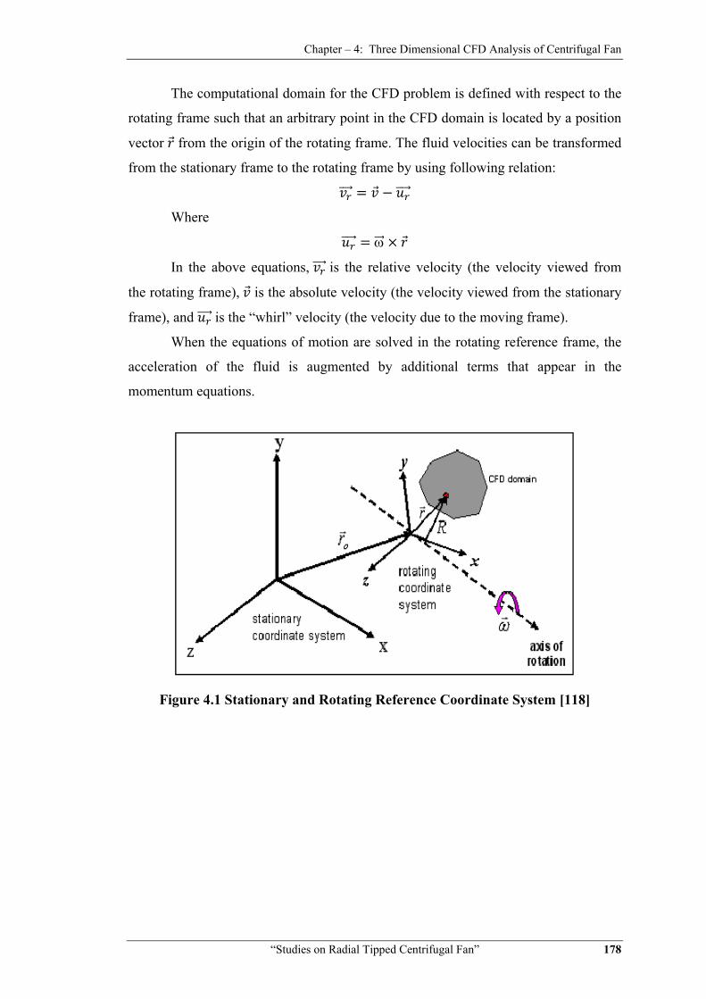
4.2.1 Equations for a moving reference frame
A coordinate system which is rotating steadily with angular velocity ω
relative to a stationary (inertial) reference frame is illustrated by Figure 4.1. The
origin of the rotating system is located by a position vector . The axis of rotation is
defined by a unit direction vector such that
ω ω
Chapter – 4: Three Dimensional CFD Analysis of Centrifugal Fan
“Studies on Radial Tipped Centrifugal Fan” 178
The computational domain for the CFD problem is defined with respect to the
rotating frame such that an arbitrary point in the CFD domain is located by a position
vector from the origin of the rotating frame. The fluid velocities can be transformed
from the stationary frame to the rotating frame by using following relation:
Where
ω
In the above equations, is the relative velocity (the velocity viewed from
the rotating frame), is the absolute velocity (the velocity viewed from the stationary
frame), and is the “whirl” velocity (the velocity due to the moving frame).
When the equations of motion are solved in the rotating reference frame, the
acceleration of the fluid is augmented by additional terms that appear in the
momentum equations.
Figure 4.1 Stationary and Rotating Reference Coordinate System [118]
Chapter – 4: Three Dimensional CFD Analysis of Centrifugal Fan
“Studies on Radial Tipped Centrifugal Fan” 179
4.2.2 Absolute velocity formulation
[66]
For the absolute velocity formulation, the ‘Reynolds-averaged Navier-Stokes’
equations (RANS) are the governing equations for a steady rotating fluid flow. For
conservation of mass it is:
ρ . ρ 0
For conservation of momentum it is:
ρ . ρ ρ ω т
For conservation of energy it is:
ρ . ρ . т .
The multiple moving reference frame (MMRF) is a steady-state approximation
in which individual cell zones move at different rotational and/or translational speeds.
The flow in each moving cell zone is solved using the moving reference frame
equations. If the zone is stationary (ω = 0), the stationary equations are used. At the
interfaces between cell zones, a local reference frame transformation is performed to
enable flow variables in one zone to be used to calculate fluxes at the boundary of the
adjacent zone.
It should be noted that the MRF approach does not account for the relative
motion of a moving zone with respect to adjacent zones (which may be moving or
stationary); the grid remains fixed for the computation. This is analogous to freezing
the motion of the moving part in a specific position and observing the instantaneous
flow field with the rotor in that position. Hence, the MRF is often referred to as the
“frozen rotor approach.” [127].
While the MRF approach is clearly an approximation, it can provide a
reasonable model of the flow for many applications. For example, the MRF model
can be used for turbomachinery applications in which rotor-stator interaction is
relatively weak, and the flow is relatively uncomplicated at the interface between the
moving and stationary zones. It can be used for mixing tank problems where impeller-
baffle interactions are also relatively weak.
Chapter – 4: Three Dimensional CFD Analysis of Centrifugal Fan
“Studies on Radial Tipped Centrifugal Fan” 180
4.2.3 Limitations of MRF approach
The interfaces separating a moving region from adjacent regions must be
oriented such that the component of the frame velocity normal to the boundary is
zero. That is, the interfaces must be surfaces of revolution about the axis of rotation
defined for the fluid zone. For a translational moving frame, the moving zone's
boundaries must be parallel to the translational velocity vector.
Multiple moving reference frames is meaningful only for steady flow.
However, FLUENT will allow to solve an unsteady flow when multiple reference
frames are being used. In this case, unsteady terms are added to all the governing
transport equations. For unsteady flows, a sliding mesh approach will yield more
meaningful results than an MRF calculation.
Particle trajectories and path lines have drawn by FLUENT uses the velocity
relative to the cell zone motion. For mass-less particles, the resulting path-lines follow
the streamlines based on relative velocity. Translational and rotational velocities are
assumed to be constant (time varying ω, vt are not allowed).
4.3 Description of Solution Algorithm
Turbulent flows are characterized by fluctuating velocity fields. These
fluctuations mix transported quantities such as momentum, energy, and species
concentration, and cause the transported quantities to fluctuate as well. Since
these fluctuations can be of small scale and high frequency, they are too
computationally expensive to simulate directly in practical engineering calculations.
Instead, the instantaneous (exact) governing equations can be time-averaged,
ensemble-averaged, or otherwise manipulated to remove the small scales, resulting in
a modified set of equations. These are computationally less expensive to solve it.
However, the modified equations contain additional unknown variables, and
additional turbulence models are needed to determine these variables in terms of
known quantities.
FLUENT provides the following choices for turbulence models:
Spalart-Allmaras model,
k-ε models,
Standard k-ε model,
Renormalization-group (RNG) k-ε model,
Chapter – 4: Three Dimensional CFD Analysis of Centrifugal Fan
“Studies on Radial Tipped Centrifugal Fan” 181
Realizable k-ε model,
3 phase k-ω models and
Shear-stress transport (SST) k-ω model.
Any single turbulence model stated above is not universally accepted as
superior for all classes of problems. The choice of turbulence model will depend on
considerations such as the physics encompassed in the flow, the level of accuracy
required, the available computational resources, and the amount of time available for
the simulation. The simplest "complete models'' of turbulence are two equation
models in which the solution of two separate transport equations allows the turbulent
velocity and length scales to be independently determined. The standard k-ε model
falls within this class and has become the workhorse of practical engineering flow
calculations in the time since it was proposed by Launder and Spalding [139].
Robustness, economy, and reasonable accuracy for a wide range of turbulent flows
explain its popularity in industrial flow and heat transfer simulations. It is a semi-
empirical model, and the derivation of the model equations relies on
phenomenological considerations and empirism. As the strengths and weaknesses of
the standard k-ε model have become known, improvements have been made to the
model to improve its performance. RNG k-ε model and the realizable k-ε model are
two of these variants available in FLUENT. The standard k-ε model is a semi
empirical model based on model transport equations for the turbulence kinetic energy
(k) and its dissipation rate (ε). The model transport equation for k is derived from the
exact equation, while the model transport equation for ε was obtained using physical
reasoning and bears little resemblance to its mathematically exact counterpart.
The realizable k-ε is a relatively recent developed model and differs from the
standard k-ε model in two important way, it contains a new formulation for the
turbulent viscosity and a new transport equation for the dissipation rate ε, has been
derived from an exact equation for the transport of the mean square vorticity
fluctuation. It is due to this fact that in the present work, realizable k-ε model is used.
Chapter – 4: Three Dimensional CFD Analysis of Centrifugal Fan
“Studies on Radial Tipped Centrifugal Fan” 182
4.3.1 Realizable k-ε model
[118]
The term “realizable” means that the model satisfies certain mathematical
constraints on the Reynolds stresses, consistent with the physics of turbulent flows.
Neither the standard k-ε model nor the RNG k-ε model is realizable. An immediate
benefit of the realizable k-ε model is that it more accurately predicts the spreading
rate of both planar and round jets. It is also likely to provide superior performance for
flows involving rotation, boundary layers under strong adverse pressure gradients,
separation, and recirculation.
Both the realizable and RNG k-ε models have shown substantial
improvements over the standard k-ε model where the flow features include strong
streamline curvature, vortices and rotation. Since the model is still relatively new, it is
not clear in exactly which instances the realizable k-ε model consistently outperforms
the RNG model. However, initial studies have shown that the realizable model
provides the best performance of all the k-ε model versions for several validations of
separated flows and flows with complex secondary flow features [66, 121].
One limitation of the realizable k-ε model is that it produces non-physical
turbulent viscosities in situations when the computational domain contains both
rotating and stationary fluid zones (e.g., multiple reference frames, rotating sliding
meshes). This is due to the fact that the realizable k-ε model includes the effects of
mean rotation in the definition of the turbulent viscosity. This extra rotation effect has
been tested on single rotating reference frame systems and showed superior behavior
over the standard k-ε model [66].
This model has been extensively validated for a wide range of flows, including
rotating homogeneous shear flows, free flows including jets and mixing layers,
channel and boundary layer flows, and separated flows. For all these cases, the
performance of the model has been found to be substantially better than that of the
standard k-ε model. The realizable k-ε model resolves the round-jet anomalies by
predicting the spreading rate for axi-symmetric jets as well as planar jets [66, 121].
Chapter – 4: Three Dimensional CFD Analysis of Centrifugal Fan
“Studies on Radial Tipped Centrifugal Fan” 183
4.4 Computational Grid
ANSYS inc. offers Gambit as pre processor software. The pre-processing
work in present course is done by using GAMBIT (Geometry and Mesh Building
Intelligent Toolkit) software. GAMBIT is very robust tool for geometry generation
and it gives total user control while doing meshing work. Allocation of nodes as per
design geometry is carried out. The co-ordinates of each node are spatially created
and then two dimensional lines and curves are generated. Later faces from lines and
then volumes from faces are generated. Volumes are identified according to required
moving and stationary zones. To create number of blades, first one blade profile is
generated and then it is copied around the z-axis in required numbers as per design.
After generating blade volumes, they are subtracted from impeller zone. For this
reason the radial and axial size of impeller is kept little higher than blades’ volume.
Adjacent stationary and moving boundaries are differentiated by using shadow wall
interface concept. To create ‘shadow wall’ interface between impeller and casing, the
volume of impeller is ‘spitted’ from volume of scroll casing. Each moving and
stationary zone is given property of fluid.
Due to complex flow structure in centrifugal fan the unstructured/hybrid grid
with tetrahedral element is recommended by few researchers [117, 118, 124].
Accordingly in present work unstructured grid/hybrid grid with tetrahedral elements is
selected. Here finer elements in impeller region are used as compared to inlet nozzle
and scroll casing as generated by commercial code GAMBIT [117].
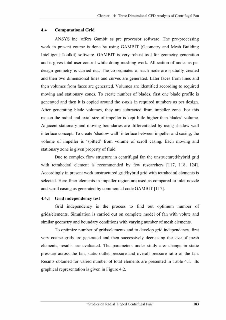
4.4.1 Grid independency test
Grid independency is the process to find out optimum number of
grids/elements. Simulation is carried out on complete model of fan with volute and
similar geometry and boundary conditions with varying number of mesh elements.
To optimize number of grids/elements and to develop grid independency, first
very coarse grids are generated and then successively decreasing the size of mesh
elements, results are evaluated. The parameters under study are: change in static
pressure across the fan, static outlet pressure and overall pressure ratio of the fan.
Results obtained for varied number of total elements are presented in Table 4.1. Its
graphical representation is given in Figure 4.2.
Chapter – 4: Three Dimensional CFD Analysis of Centrifugal Fan
“Studies on Radial Tipped Centrifugal Fan” 184
Table 4.1 Grid Independency Test
Mesh No. of Mesh Elements
∆P Static (Pa)
Static Outlet Pressure (Pa) Pressure Ratio
a 219210 797.665 657.97 1.00788
b 419633 834.69 681.59 1.00825
c 869068 834.24 679.67 1.00824
d 1934222 833.37 679.04 1.008237
Figure 4.2 Graphical Representation of Mesh Independency Test
In present case, it is clearly seen from Figure 4.2 and Table 4.1 that mesh ‘b’
results are more accurate as compared to mesh ‘a’ result. Further it is found that the
relative deviation of the static pressure rise, static outlet pressure and pressure ratio
between mesh ‘b’ and ‘c’ is less than 1%. Mesh ‘c’ and ‘d’ yield similar results.
Chapter – 4: Three Dimensional CFD Analysis of Centrifugal Fan
“Studies on Radial Tipped Centrifugal Fan” 185
Further increase in mesh elements will not affect accuracy, simulation results. Hence
mesh ‘b’ with 419633 mesh elements is accepted for all further simulations to save
simulation time.
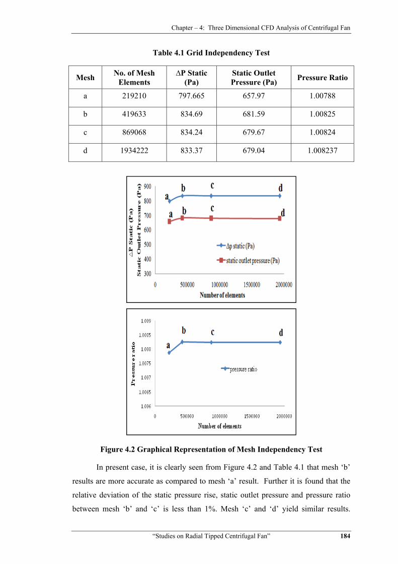
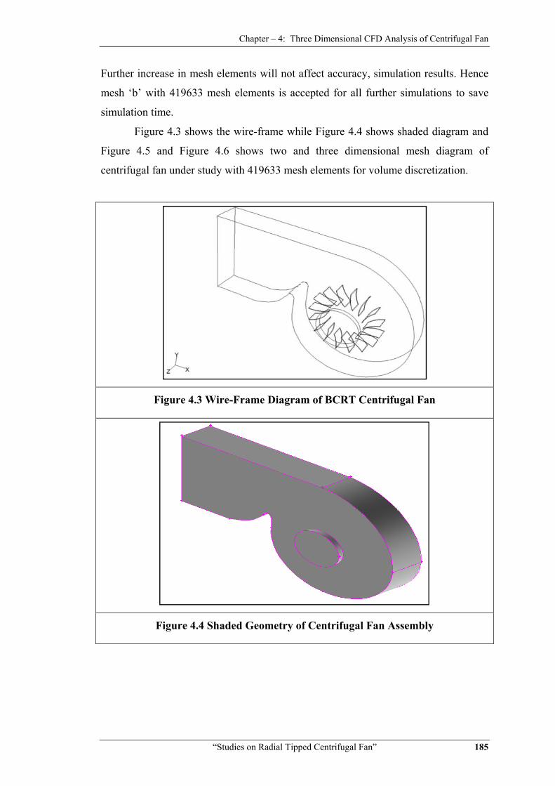
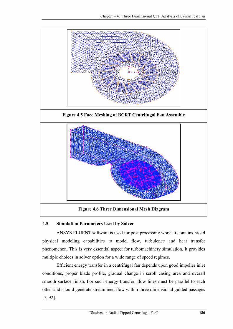
Figure 4.3 shows the wire-frame while Figure 4.4 shows shaded diagram and
Figure 4.5 and Figure 4.6 shows two and three dimensional mesh diagram of
centrifugal fan under study with 419633 mesh elements for volume discretization.
Figure 4.3 Wire-Frame Diagram of BCRT Centrifugal Fan
Figure 4.4 Shaded Geometry of Centrifugal Fan Assembly
Chapter – 4: Three Dimensional CFD Analysis of Centrifugal Fan
“Studies on Radial Tipped Centrifugal Fan” 186
Figure 4.5 Face Meshing of BCRT Centrifugal Fan Assembly
Figure 4.6 Three Dimensional Mesh Diagram
4.5 Simulation Parameters Used by Solver
ANSYS FLUENT software is used for post processing work. It contains broad
physical modeling capabilities to model flow, turbulence and heat transfer
phenomenon. This is very essential aspect for turbomachinery simulation. It provides
multiple choices in solver option for a wide range of speed regimes.
Efficient energy transfer in a centrifugal fan depends upon good impeller inlet
conditions, proper blade profile, gradual change in scroll casing area and overall
smooth surface finish. For such energy transfer, flow lines must be parallel to each
other and should generate streamlined flow within three dimensional guided passages
[7, 92].

Chapter – 4: Three Dimensional CFD Analysis of Centrifugal Fan
“Studies on Radial Tipped Centrifugal Fan” 187
The inlet nozzle and scroll casing are stationary zones and impeller is a
moving zone. Being steady flow and very low pressure ratio in this case, moving
reference frame (MRF) approach is used to impose rotational field to impeller zone of
centrifugal fan[113]. The blades are moving with a same rotational velocity as
impeller zone by giving moving wall condition with zero relative rotational speed to
adjacent cell zone. Shadow wall method is used as interior surface to create
continuous flow path between moving and stationary zones.
In the centrifugal fans, the three-dimensional motion of the air is thought to be
the incompressible and steady flow. Three dimensional simulation is carried out
using ‘Reynolds-averaged Navier-Stokes’ equations (RANS) and ‘Realizable k-ε
model’. As the fluid in a state of turbulence, the Realizable k −ε model was selected
as the turbulence model to give superior performance for flows involving rotation,
separation and recirculation. The ‘standard’ wall function is used to resolve wall
flows. The ‘SIMPLE’ algorithm is used for coupling pressure and velocity [118, 122,
112]. Turbulent kinetic energy and dissipation of turbulence uses function of second-
order discrete upwind.
Mass flow rate at nozzle inlet is used as inlet boundary condition. Zero
gradient outflow condition is used at casing outlet. This is done for fully developed
flow conditions. At inlet boundary condition, 5% turbulent intensity and 0.5 turbulent
length scale is applied [118]. This is calculated based on cube root of domain volume
and used for turbulence specifications. ‘No-slip’ boundary condition is used for all
walls. The discharge at nozzle inlet at each step of rotational speed of impeller is
varied by varying input boundary condition of inlet mass flow rate.
Present simulation work is carried out on the backward and forward curved
radial tipped centrifugal fans designed as per unified design methodology, as
explained in chapter 3. The factors that impact fan’s performance are coupled with
each other. Various factors have a combined action together on the fan performance.
This work takes the efficiency η as a maximizations goal, and takes the number of
blade Z, speed of impeller rotation N and the volume flow rate Q as the variable
quantity, and constructs the optimized mathematical model:
, ,
In the model, f (x, y, z) represents the objective function of efficiency η, and
parameters x, y and z separately represent the number of blade, speed of rotation and
Chapter – 4: Three Dimensional CFD Analysis of Centrifugal Fan
“Studies on Radial Tipped Centrifugal Fan” 188
the volume flow for backward and forward curved radial tipped centrifugal fans
designed as per unified design methodology.
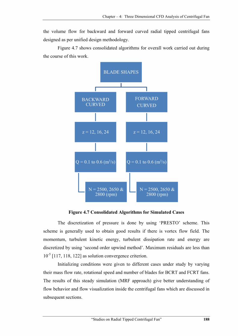
Figure 4.7 shows consolidated algorithms for overall work carried out during
the course of this work.
Figure 4.7 Consolidated Algorithms for Simulated Cases
The discretization of pressure is done by using ‘PRESTO’ scheme. This
scheme is generally used to obtain good results if there is vortex flow field. The
momentum, turbulent kinetic energy, turbulent dissipation rate and energy are
discretized by using ‘second order upwind method’. Maximum residuals are less than
10-5 [117, 118, 122] as solution convergence criterion.
Initializing conditions were given to different cases under study by varying
their mass flow rate, rotational speed and number of blades for BCRT and FCRT fans.
The results of this steady simulation (MRF approach) give better understanding of
flow behavior and flow visualization inside the centrifugal fans which are discussed in
subsequent sections.
BLADE SHAPES
BACKWARD CURVED
z = 12, 16, 24
Q = 0.1 to 0.6 (m3/s)
N = 2500, 2650 & 2800 (rpm)
FORWARD CURVED
z = 12, 16, 24
Q = 0.1 to 0.6 (m3/s)
N = 2500, 2650 & 2800 (rpm)
Chapter – 4: Three Dimensional CFD Analysis of Centrifugal Fan
“Studies on Radial Tipped Centrifugal Fan” 189
4.6 Numerical Flow Analysis of Backward Curved and Forward Curved Radial Tipped Blade Centrifugal Fan
Qualitative and quantitative simulation result analysis of the flow in radial
tipped backward curved blade (BCRT) and forward curved blade (FCRT) centrifugal
fan with varying discharge, speed and number of blades is presented herein.
Discharge is varied between 0.1 to 0.6 m3/s with the increment of 0.1 m3/s. Speed of
rotation is varied as 2500, 2650 and 2800 rpm, while number of blades is varied as 12,
16 and 24 for each case stated above.
Efficient energy transfer in a centrifugal fan depends upon proper blade
profile, gradual change in area of scroll casing and smooth surface finish within
impeller vane passage. Flow lines must be parallel to each other and should generate
streamlined flow within three dimensional passages [13, 26].
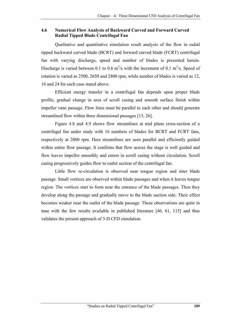
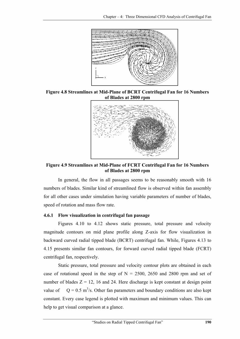
Figure 4.8 and 4.9 shows flow streamlines at mid plane cross-section of a
centrifugal fan under study with 16 numbers of blades for BCRT and FCRT fans,
respectively at 2800 rpm. Here streamlines are seen parallel and efficiently guided
within entire flow passage. It confirms that flow across the stage is well guided and
flow leaves impeller smoothly and enters in scroll casing without circulation. Scroll
casing progressively guides flow to outlet section of the centrifugal fan.
Little flow re-circulation is observed near tongue region and inter blade
passage. Small vortices are observed within blade passages and when it leaves tongue
region. The vortices start to form near the entrance of the blade passages. Then they
develop along the passage and gradually move to the blade suction side. Their effect
becomes weaker near the outlet of the blade passage. These observations are quite in
tune with the few results available in published literature [46, 61, 115] and thus
validates the present approach of 3-D CFD simulation.
Chapter – 4: Three Dimensional CFD Analysis of Centrifugal Fan
“Studies on Radial Tipped Centrifugal Fan” 190
Figure 4.8 Streamlines at Mid-Plane of BCRT Centrifugal Fan for 16 Numbers
of Blades at 2800 rpm
Figure 4.9 Streamlines at Mid-Plane of FCRT Centrifugal Fan for 16 Numbers
of Blades at 2800 rpm In general, the flow in all passages seems to be reasonably smooth with 16
numbers of blades. Similar kind of streamlined flow is observed within fan assembly
for all other cases under simulation having variable parameters of number of blades,
speed of rotation and mass flow rate.
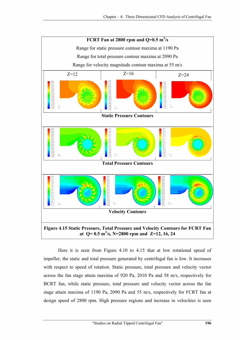
4.6.1 Flow visualization in centrifugal fan passage
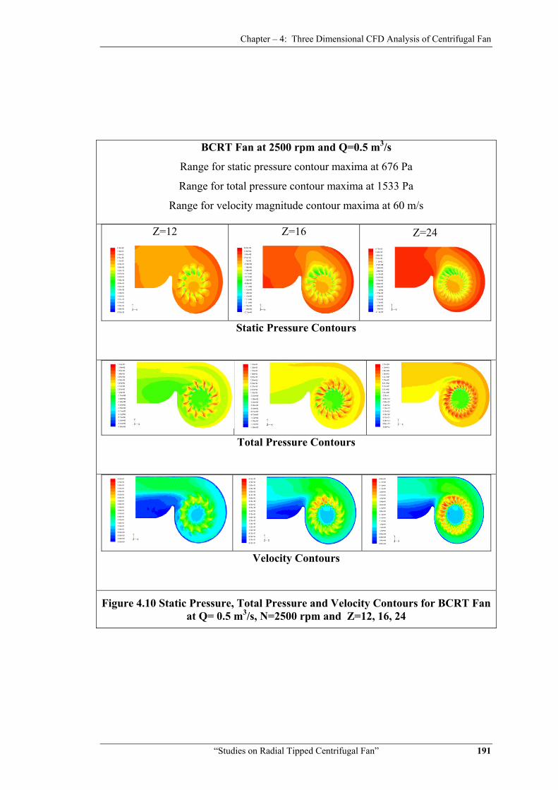
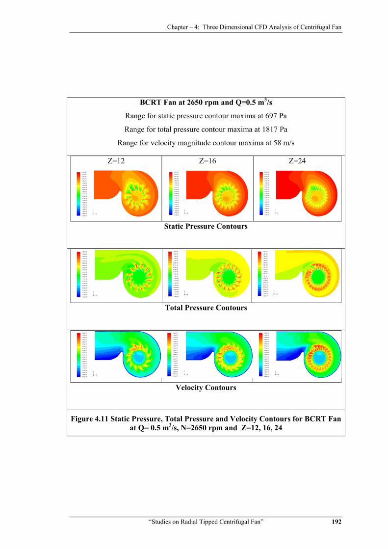
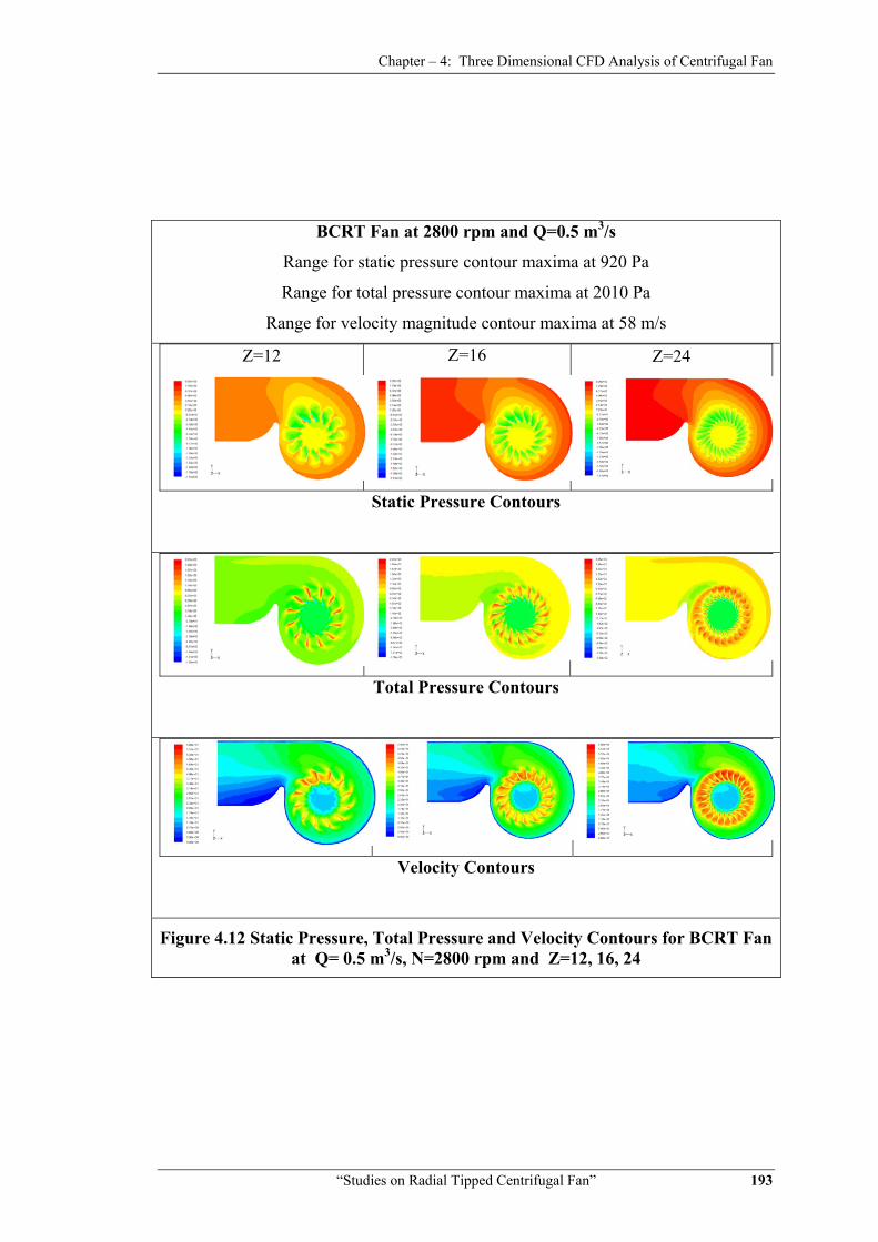
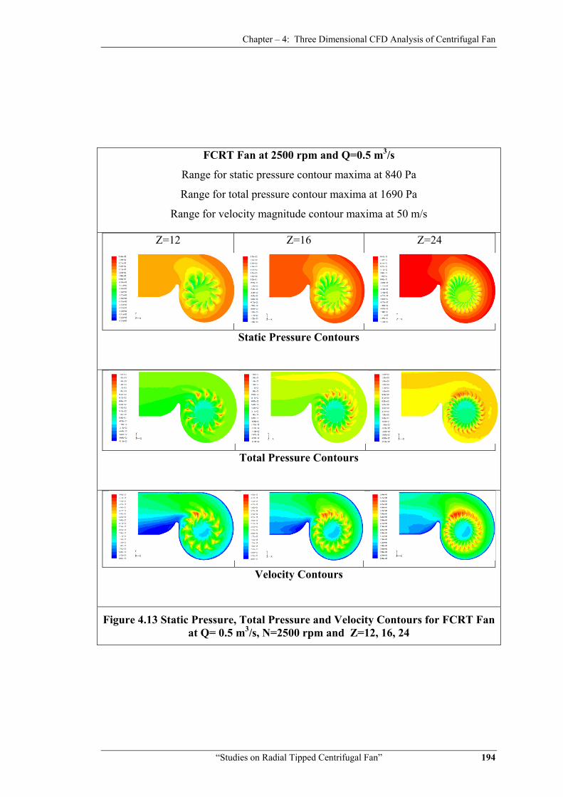
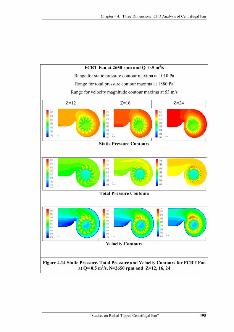
Figures 4.10 to 4.12 shows static pressure, total pressure and velocity
magnitude contours on mid plane profile along Z-axis for flow visualization in
backward curved radial tipped blade (BCRT) centrifugal fan. While, Figures 4.13 to
4.15 presents similar fan contours, for forward curved radial tipped blade (FCRT)
centrifugal fan, respectively.
Static pressure, total pressure and velocity contour plots are obtained in each
case of rotational speed in the step of N = 2500, 2650 and 2800 rpm and set of
number of blades Z = 12, 16 and 24. Here discharge is kept constant at design point
value of Q = 0.5 m3/s. Other fan parameters and boundary conditions are also kept
constant. Every case legend is plotted with maximum and minimum values. This can
help to get visual comparison at a glance.
Chapter – 4: Three Dimensional CFD Analysis of Centrifugal Fan
“Studies on Radial Tipped Centrifugal Fan” 191
BCRT Fan at 2500 rpm and Q=0.5 m3/s
Range for static pressure contour maxima at 676 Pa
Range for total pressure contour maxima at 1533 Pa
Range for velocity magnitude contour maxima at 60 m/s
Z=12
Z=16 Z=24
Static Pressure Contours
Total Pressure Contours
Velocity Contours
Figure 4.10 Static Pressure, Total Pressure and Velocity Contours for BCRT Fan at Q= 0.5 m3/s, N=2500 rpm and Z=12, 16, 24
Chapter – 4: Three Dimensional CFD Analysis of Centrifugal Fan
“Studies on Radial Tipped Centrifugal Fan” 192
BCRT Fan at 2650 rpm and Q=0.5 m3/s
Range for static pressure contour maxima at 697 Pa
Range for total pressure contour maxima at 1817 Pa
Range for velocity magnitude contour maxima at 58 m/s
Z=12
Z=16
Z=24
Static Pressure Contours
Total Pressure Contours
Velocity Contours
Figure 4.11 Static Pressure, Total Pressure and Velocity Contours for BCRT Fan at Q= 0.5 m3/s, N=2650 rpm and Z=12, 16, 24
Chapter – 4: Three Dimensional CFD Analysis of Centrifugal Fan
“Studies on Radial Tipped Centrifugal Fan” 193
BCRT Fan at 2800 rpm and Q=0.5 m3/s
Range for static pressure contour maxima at 920 Pa
Range for total pressure contour maxima at 2010 Pa
Range for velocity magnitude contour maxima at 58 m/s
Z=12 Z=16 Z=24
Static Pressure Contours
Total Pressure Contours
Velocity Contours
Figure 4.12 Static Pressure, Total Pressure and Velocity Contours for BCRT Fan at Q= 0.5 m3/s, N=2800 rpm and Z=12, 16, 24
Chapter – 4: Three Dimensional CFD Analysis of Centrifugal Fan
“Studies on Radial Tipped Centrifugal Fan” 194
FCRT Fan at 2500 rpm and Q=0.5 m3/s
Range for static pressure contour maxima at 840 Pa
Range for total pressure contour maxima at 1690 Pa
Range for velocity magnitude contour maxima at 50 m/s
Z=12 Z=16 Z=24
Static Pressure Contours
Total Pressure Contours
Velocity Contours
Figure 4.13 Static Pressure, Total Pressure and Velocity Contours for FCRT Fan at Q= 0.5 m3/s, N=2500 rpm and Z=12, 16, 24
Chapter – 4: Three Dimensional CFD Analysis of Centrifugal Fan
“Studies on Radial Tipped Centrifugal Fan” 195
FCRT Fan at 2650 rpm and Q=0.5 m3/s
Range for static pressure contour maxima at 1010 Pa
Range for total pressure contour maxima at 1880 Pa
Range for velocity magnitude contour maxima at 53 m/s
Z=12 Z=16 Z=24
Static Pressure Contours
Total Pressure Contours
Velocity Contours
Figure 4.14 Static Pressure, Total Pressure and Velocity Contours for FCRT Fan at Q= 0.5 m3/s, N=2650 rpm and Z=12, 16, 24
Chapter – 4: Three Dimensional CFD Analysis of Centrifugal Fan
“Studies on Radial Tipped Centrifugal Fan” 196
FCRT Fan at 2800 rpm and Q=0.5 m3/s
Range for static pressure contour maxima at 1190 Pa
Range for total pressure contour maxima at 2090 Pa
Range for velocity magnitude contour maxima at 55 m/s
Z=12 Z=16 Z=24
Static Pressure Contours
Total Pressure Contours
Velocity Contours
Figure 4.15 Static Pressure, Total Pressure and Velocity Contours for FCRT Fan at Q= 0.5 m3/s, N=2800 rpm and Z=12, 16, 24
Here it is seen from Figure 4.10 to 4.15 that at low rotational speed of
impeller, the static and total pressure generated by centrifugal fan is low. It increases
with respect to speed of rotation. Static pressure, total pressure and velocity vector
across the fan stage attain maxima of 920 Pa, 2010 Pa and 58 m/s, respectively for
BCRT fan, while static pressure, total pressure and velocity vector across the fan
stage attain maxima of 1190 Pa, 2090 Pa and 55 m/s, respectively for FCRT fan at
design speed of 2800 rpm. High pressure regions and increase in velocities is seen
Chapter – 4: Three Dimensional CFD Analysis of Centrifugal Fan
“Studies on Radial Tipped Centrifugal Fan” 197
around impeller outlet. Pressure and velocity increases with increase in impeller speed
and number of blades. Growth in velocity magnitude in impeller blade passages is
clearly seen. Simulated results reveals that 834.7 Pa average static pressure rise is
observed for the BCRT and 1106.7 Pa for the FCRT centrifugal fan for 16 number of
blades across the stage. This shows 15% and 11% deviation between design point
static pressure rise of 981.2 Pa for BCRT and FCRT fan, respectively, by keeping all
other parameters constant.
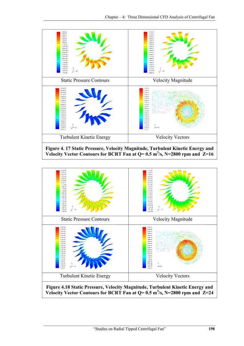
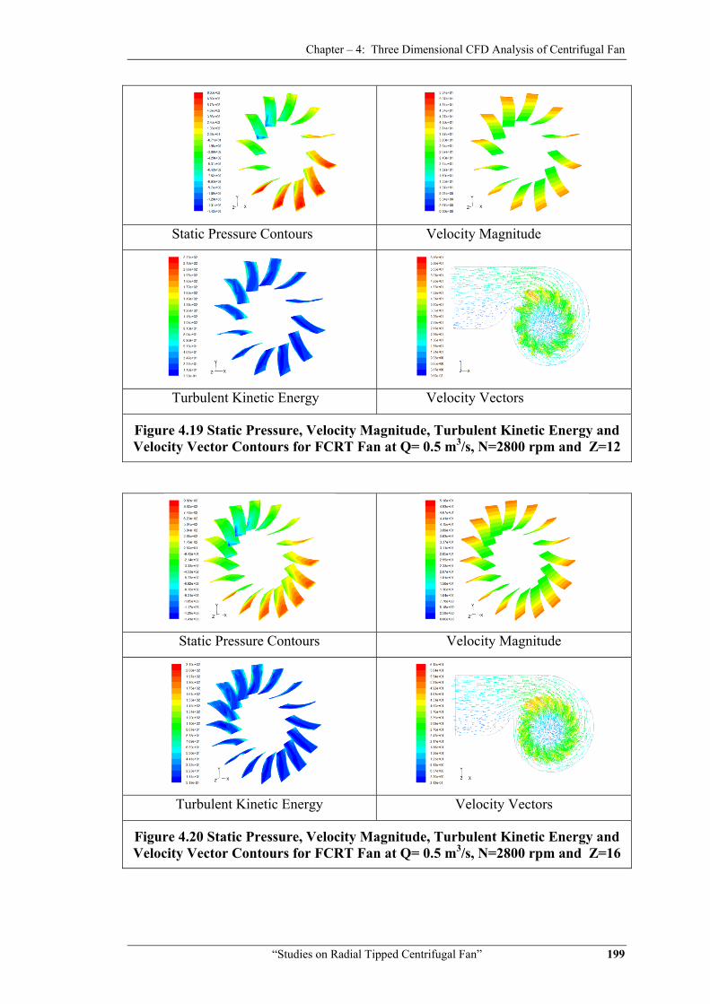
4.6.2 Flow visualization on blade surfaces and velocity vectors
Post-processing three dimensional simulation results are presented in Figure
4.16 to 4.18 for flow visualization on suction and discharge side blade surfaces of
BCRT fan and velocity vectors within entire flow passage, while, Figures 4.19 to 4.21
presents similar three dimensional simulation for forward curved radial tipped blade
(FCRT) centrifugal fan, respectively. It is represented in the form of contours of static
pressure, velocity magnitude, turbulent kinetic energy and velocity vectors. Various
contour plots are obtained for rotational speed of 2800 rpm and number of blades in
the steps of 12, 16 and 24. Here discharge is kept constant at design value of Q=0.5
m3/s.
Static Pressure Contours Velocity Magnitude
Turbulent Kinetic Energy Velocity Vectors
Figure 4.16 Static Pressure, Velocity Magnitude, Turbulent Kinetic Energy and Velocity Vector Contours for BCRT Fan at Q= 0.5 m3/s, N=2800 rpm and Z=12
Chapter – 4: Three Dimensional CFD Analysis of Centrifugal Fan
“Studies on Radial Tipped Centrifugal Fan” 198
Static Pressure Contours Velocity Magnitude
Turbulent Kinetic Energy Velocity Vectors
Figure 4. 17 Static Pressure, Velocity Magnitude, Turbulent Kinetic Energy and Velocity Vector Contours for BCRT Fan at Q= 0.5 m3/s, N=2800 rpm and Z=16
Static Pressure Contours Velocity Magnitude
Turbulent Kinetic Energy Velocity Vectors
Figure 4.18 Static Pressure, Velocity Magnitude, Turbulent Kinetic Energy and Velocity Vector Contours for BCRT Fan at Q= 0.5 m3/s, N=2800 rpm and Z=24
Chapter – 4: Three Dimensional CFD Analysis of Centrifugal Fan
“Studies on Radial Tipped Centrifugal Fan” 199
Static Pressure Contours Velocity Magnitude
Turbulent Kinetic Energy Velocity Vectors
Figure 4.19 Static Pressure, Velocity Magnitude, Turbulent Kinetic Energy and Velocity Vector Contours for FCRT Fan at Q= 0.5 m3/s, N=2800 rpm and Z=12
Static Pressure Contours Velocity Magnitude
Turbulent Kinetic Energy Velocity Vectors
Figure 4.20 Static Pressure, Velocity Magnitude, Turbulent Kinetic Energy and Velocity Vector Contours for FCRT Fan at Q= 0.5 m3/s, N=2800 rpm and Z=16
Chapter – 4: Three Dimensional CFD Analysis of Centrifugal Fan
“Studies on Radial Tipped Centrifugal Fan” 200
Static Pressure Contours Velocity Magnitude
Turbulent Kinetic Energy Velocity Vectors
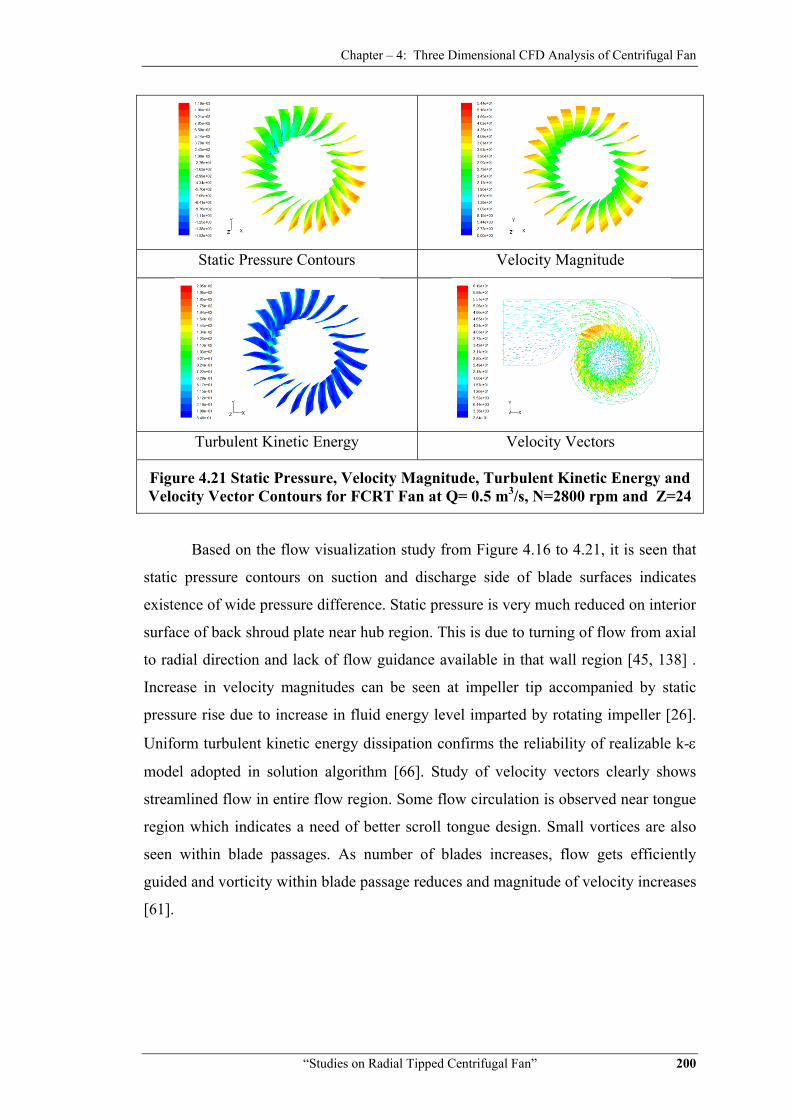
Figure 4.21 Static Pressure, Velocity Magnitude, Turbulent Kinetic Energy and Velocity Vector Contours for FCRT Fan at Q= 0.5 m3/s, N=2800 rpm and Z=24
Based on the flow visualization study from Figure 4.16 to 4.21, it is seen that
static pressure contours on suction and discharge side of blade surfaces indicates
existence of wide pressure difference. Static pressure is very much reduced on interior
surface of back shroud plate near hub region. This is due to turning of flow from axial
to radial direction and lack of flow guidance available in that wall region [45, 138] .
Increase in velocity magnitudes can be seen at impeller tip accompanied by static
pressure rise due to increase in fluid energy level imparted by rotating impeller [26].
Uniform turbulent kinetic energy dissipation confirms the reliability of realizable k-ε
model adopted in solution algorithm [66]. Study of velocity vectors clearly shows
streamlined flow in entire flow region. Some flow circulation is observed near tongue
region which indicates a need of better scroll tongue design. Small vortices are also
seen within blade passages. As number of blades increases, flow gets efficiently
guided and vorticity within blade passage reduces and magnitude of velocity increases
[61].
Chapter – 4: Three Dimensional CFD Analysis of Centrifugal Fan
“Studies on Radial Tipped Centrifugal Fan” 201
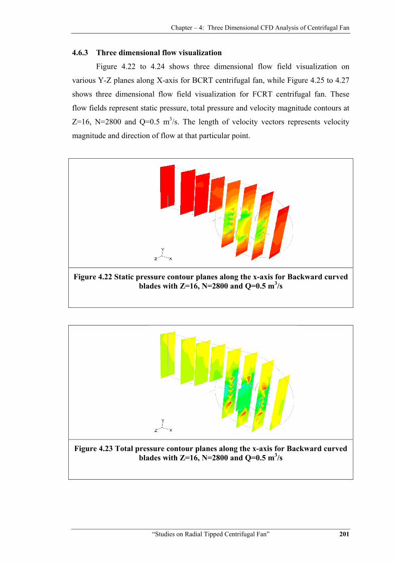
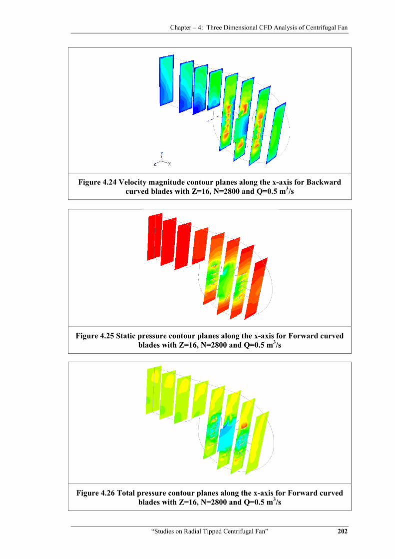
4.6.3 Three dimensional flow visualization
Figure 4.22 to 4.24 shows three dimensional flow field visualization on
various Y-Z planes along X-axis for BCRT centrifugal fan, while Figure 4.25 to 4.27
shows three dimensional flow field visualization for FCRT centrifugal fan. These
flow fields represent static pressure, total pressure and velocity magnitude contours at
Z=16, N=2800 and Q=0.5 m3/s. The length of velocity vectors represents velocity
magnitude and direction of flow at that particular point.
Figure 4.22 Static pressure contour planes along the x-axis for Backward curved blades with Z=16, N=2800 and Q=0.5 m3/s
Figure 4.23 Total pressure contour planes along the x-axis for Backward curved blades with Z=16, N=2800 and Q=0.5 m3/s
Chapter – 4: Three Dimensional CFD Analysis of Centrifugal Fan
“Studies on Radial Tipped Centrifugal Fan” 202
Figure 4.24 Velocity magnitude contour planes along the x-axis for Backward curved blades with Z=16, N=2800 and Q=0.5 m3/s
Figure 4.25 Static pressure contour planes along the x-axis for Forward curved blades with Z=16, N=2800 and Q=0.5 m3/s
Figure 4.26 Total pressure contour planes along the x-axis for Forward curved blades with Z=16, N=2800 and Q=0.5 m3/s
Chapter – 4: Three Dimensional CFD Analysis of Centrifugal Fan
“Studies on Radial Tipped Centrifugal Fan” 203
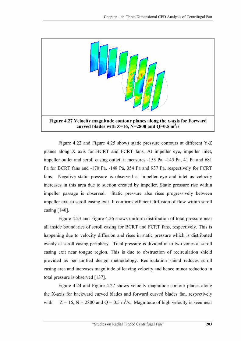
Figure 4.27 Velocity magnitude contour planes along the x-axis for Forward curved blades with Z=16, N=2800 and Q=0.5 m3/s
Figure 4.22 and Figure 4.25 shows static pressure contours at different Y-Z
planes along X axis for BCRT and FCRT fans. At impeller eye, impeller inlet,
impeller outlet and scroll casing outlet, it measures -153 Pa, -145 Pa, 41 Pa and 681
Pa for BCRT fans and -170 Pa, -148 Pa, 354 Pa and 937 Pa, respectively for FCRT
fans. Negative static pressure is observed at impeller eye and inlet as velocity
increases in this area due to suction created by impeller. Static pressure rise within
impeller passage is observed. Static pressure also rises progressively between
impeller exit to scroll casing exit. It confirms efficient diffusion of flow within scroll
casing [140].
Figure 4.23 and Figure 4.26 shows uniform distribution of total pressure near
all inside boundaries of scroll casing for BCRT and FCRT fans, respectively. This is
happening due to velocity diffusion and rises in static pressure which is distributed
evenly at scroll casing periphery. Total pressure is divided in to two zones at scroll
casing exit near tongue region. This is due to obstruction of recirculation shield
provided as per unified design methodology. Recirculation shield reduces scroll
casing area and increases magnitude of leaving velocity and hence minor reduction in
total pressure is observed [137].
Figure 4.24 and Figure 4.27 shows velocity magnitude contour planes along
the X-axis for backward curved blades and forward curved blades fan, respectively
with Z = 16, N = 2800 and Q = 0.5 m3/s. Magnitude of high velocity is seen near
Chapter – 4: Three Dimensional CFD Analysis of Centrifugal Fan
“Studies on Radial Tipped Centrifugal Fan” 204
impeller exit. This phenomenon occurs as fluid leaving the impeller gets energy and
increases its velocity and static pressure level. Thereafter velocities reduce within
scroll casing. Again two zones of velocities of different magnitudes are observed near
scroll casing exit due to obstruction of recirculation shield [137].
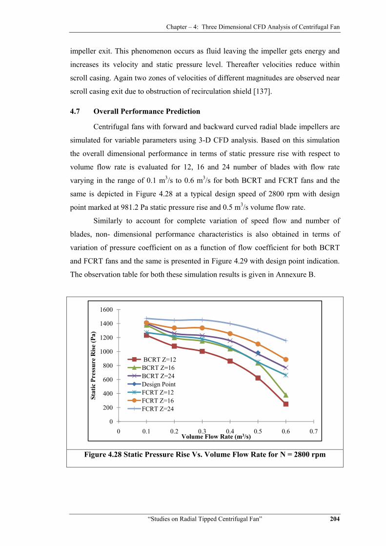
4.7 Overall Performance Prediction
Centrifugal fans with forward and backward curved radial blade impellers are
simulated for variable parameters using 3-D CFD analysis. Based on this simulation
the overall dimensional performance in terms of static pressure rise with respect to
volume flow rate is evaluated for 12, 16 and 24 number of blades with flow rate
varying in the range of 0.1 m3/s to 0.6 m3/s for both BCRT and FCRT fans and the
same is depicted in Figure 4.28 at a typical design speed of 2800 rpm with design
point marked at 981.2 Pa static pressure rise and 0.5 m3/s volume flow rate.
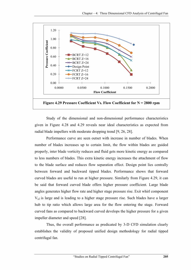
Similarly to account for complete variation of speed flow and number of
blades, non- dimensional performance characteristics is also obtained in terms of
variation of pressure coefficient on as a function of flow coefficient for both BCRT
and FCRT fans and the same is presented in Figure 4.29 with design point indication.
The observation table for both these simulation results is given in Annexure B.
Figure 4.28 Static Pressure Rise Vs. Volume Flow Rate for N = 2800 rpm
0
200
400
600
800
1000
1200
1400
1600
0 0.1 0.2 0.3 0.4 0.5 0.6 0.7
Stat
ic P
ress
ure
Ris
e (P
a)
Volume Flow Rate (m3/s)
BCRT Z=12BCRT Z=16BCRT Z=24Design PointFCRT Z=12FCRT Z=16FCRT Z=24
Chapter – 4: Three Dimensional CFD Analysis of Centrifugal Fan
“Studies on Radial Tipped Centrifugal Fan” 205
Figure 4.29 Pressure Coefficient Vs. Flow Coefficient for N = 2800 rpm
Study of the dimensional and non-dimensional performance characteristics
given in Figure 4.28 and 4.29 reveals near ideal characteristics as expected from
radial blade impellers with moderate dropping trend [9, 26, 28].
Performance curve are seen outset with increase in number of blades. When
number of blades increases up to certain limit, the flow within blades are guided
properly, inter blade vorticity reduces and fluid gets more kinetic energy as compared
to less numbers of blades. This extra kinetic energy increases the attachment of flow
to the blade surface and reduces flow separation effect. Design point lies centrally
between forward and backward tipped blades. Performance shows that forward
curved blades are useful to run at higher pressure. Similarly from Figure 4.29, it can
be said that forward curved blade offers higher pressure coefficient. Large blade
angles generates higher flow rate and higher stage pressure rise. Exit whirl component
Vu2 is large and is leading to a higher stage pressure rise. Such blades have a larger
hub to tip ratio which allows large area for the flow entering the stage. Forward
curved fans as compared to backward curved develops the higher pressure for a given
impeller diameter and speed [28].
Thus, the overall performance as predicated by 3-D CFD simulation clearly
establishes the validity of proposed unified design methodology for radial tipped
centrifugal fan.
0.00
0.20
0.40
0.60
0.80
1.00
1.20
0.0000 0.0500 0.1000 0.1500 0.2000
Pres
sure
Coe
ffic
ient
Flow Coefficient
BCRT Z=12BCRT Z=16BCRT Z=24Design PointFCRT Z=12FCRT Z=16FCRT Z=24
Chapter – 4: Three Dimensional CFD Analysis of Centrifugal Fan
“Studies on Radial Tipped Centrifugal Fan” 206
4.8 Closure
The results of numerical simulation for centrifugal fan assuming steady and
incompressible flow using MRF approach gives successful insight for flow
visualization. After critical evaluation of results obtained from all simulated cases and
comparing it with designed and experimental data available for backward and forward
curved radial tipped centrifugal fans under variable speed, volume flow rate and
numbers of blades, following conclusions are derived.
(i) Energy transfer from impeller to fluid is seen by pressure and velocity
contours within all blade passages. Low and high pressure regions along
suction and pressure side of a blade are visualized by numerical analysis.
Energy transfer from impeller to fluid is also confirmed by pressure and
velocity contours within blade passage [14].
(ii) Jet and wakes are observed in the vicinity of tongue region. The flow
phenomenon of recirculation near tongue region is confirmed by numerical
analysis as shown in stream line diagram given in Figure numbers 4.8 and 4.9.
Pressure pulsations are observed at impeller outlet near tongue region. Hence
design of tongue is very important to reduce back flow and recirculation. It
shows that design of tongue is very much important in fan design to reduce
back flow and recirculation. These observations are quite in tune with the
observations of [46, 61, 115] and others, and thereby establishes the validity of
present 3-D CFD approach.
(iii) The relative velocity in the blade passage becomes more uniform due to
proper guidance as number of blades increases, and hence wakes regions
decreases. This could reduce noise generated due to wake formation.
Formation of wake region is one of the major contributors to the fan losses.
Further increase in number of blades would deteriorate the fan performance
and boundary layer effects may become dominant [66].
(iv) Static pressure contours at different Y-Z planes along X axis for BCRT fan
reveals that, at impeller eye, impeller inlet, impeller outlet and scroll casing
outlet, static pressure measures are -153 Pa, -145 Pa, 41 Pa and 681 Pa,
respectively. There is 834.7 Pa average static pressure rise is observed for 16
number of blades across the stage. This shows 15% deviation between design
Chapter – 4: Three Dimensional CFD Analysis of Centrifugal Fan
“Studies on Radial Tipped Centrifugal Fan” 207
point static pressure rise of 981.2 Pa for 16 numbers of blades and numerical
results as obtained by keeping all other parameters constant. While in scroll
casing, static pressure rises from 250 Pa to 804 Pa. Rise in static pressure
indicates efficient diffusion of flow. Fluid leaves casing at 11.32 m/s velocity.
(v) Static pressure contours at different Y-Z planes along X axis for FCRT fan
reveals that, at impeller eye, impeller inlet, impeller outlet and scroll casing
outlet, static pressure measures are -170 Pa, -148 Pa, 354 Pa and 937 Pa,
respectively. There is 1106.7 Pa average static pressure rise is observed for 16
number of blades across the stage. This shows 11% deviation between design
point static pressure rise of 981.2 Pa for 16 numbers of blades and numerical
results as obtained by keeping all other parameters constant. While in scroll
casing, static pressure rises from 423 Pa to 1131 Pa. Rise in static pressure
indicates efficient diffusion of flow. Fluid leaves casing at 11.23 m/s velocity.
(vi) The overall dimensional and non-dimensional performance characteristics as
predicted by 3-D CFD analysis for FCRT and BCRT fans with varying flow,
speed and number of blades indicate near ideal performance characteristics as
expected from radial tipped centrifugal fans. It also shows achievement of
design point performance within acceptable limits. Further forward curved
radial tipped fan indicates higher static pressure gradient as compared to
backward curved centrifugal fan. The nature of curves obtained after
simulation study closely follows trend of standard performance curves [9, 26
and 28].
Thus, it may be stated that looking to the uncertainties in 3-D CFD analysis as
discussed by [35] and others [113, 121], the respective deviation of 15% and
11% in stage pressure rise at design flow rate of 0.5 m3/s and rotational speed
of 2800 rpm for BCRT and FCRT fans with 16 number of blade may be
considered as acceptable. Further present 3-D CFD simulation of BCRT and
FCRT fans designed as per proposed unified design methodology shows the
capabilities of these fans to offer near ideal and design point performance with
16 numbers of blades.
This means that the proposed unified design methodology for radial tipped
centrifugal fan may be treated as numerically validated design.