The Roots of the Industrial Revolution:

Political Institutions or (Socially Embedded)

Know-How?

Scott F Abramson∗ & Carles Boix†

November 26, 2014

Abstract

In this paper we reassess the nature and causes of growth (measured through urbanization aswell as nineteenth-century per capita income) in Europe from around 1200 to 1900. Employinga comprehensive dataset for the European continent that includes biogeographic features andurbanization data (1200-1800), per capita income data in the second half of the 19th century,location of proto-industrial textile and metallurgic centers and political institutions, we show,in the first place, that the process of economic take-off (and of a growing economic divergenceacross Europe) was caused by the early emergence and growth of cities and urban clusters inan European north-south corridor that broadly runs from southern England to northern Italy.In contrast to previous findings in the institutionalist literature, we show, in the second place,that the fortunes of parliamentary institutions in early modern Europe played a small part inthe success of the industrial revolution. Finally, we claim that growth happened endogenously,taking place in those territories that had a strong proto-industrial base, often regardless of theabsence of executive constraints, and easy access to energy resources.

∗Department of Politics, Princeton University. sabramso@princeton.edu†Department of Politics & WWS, Princeton University. cboix@princeton.edu

1

Two broad features define the economic history of Europe in the last millennium: one, sustained

growth, slowly at first and then at an accelerating rate after 1750; two, increasing income divergence

within Europe. According to admittedly crude estimates, GDP per capita ranged from a maximum

of $468 to a minimum of $400 (in 1990 International Geary-Khamis dollars) in Europe around the

year 1,000 (Maddison 2003). Half a millennium later, that range had widened from a minimum of

$433 in Albania to a maximum of $1,100 in Italy.1 By 1850, with the industrial revolution in full

swing in England, the maximum European per capita income had experienced a five-fold increase to

almost $2,500. Meanwhile, in the poorest areas of Europe, per capita incomes had not experienced

any significant growth.

There is no dearth of theories to explain how parts of Europe managed to escape from a

pre-industrial, Malthusian world through a long period of sustained growth. Endogenous growth

theories see economic development as the outcome of a self-generating process of learning-by-doing

and of technological innovation, arguably shaped by geographical factors (Sachs and Warner 1997)

and/or population size (Kremer 1993). Most of the current literature, however, traces growth back

to a particular configuration of institutions ranging from the presence of formal structures such as

constitutional checks and balances and constraints on the executive (North and Weingast 1989) to

social norms of cooperation and culture (North 1990, Putnam 1993, Tabellini 2010).

Both strands of the literature are beset by important theoretical and empirical gaps. Insti-

tutionalists do not endogenize the emergence of institutions, mostly tracing them back to some

unidentified critical historical juncture.2 On the other hand, endogenous growth models do not

specify with much precision the mechanisms through which economic growth takes place (in some

places but not in others). Empirically, there are similar deficiencies. Most historical work on

modern growth has been conducted by economic historians who have emphasized the analysis of

a particular case or the comparison of a few cases with Britain normally included as a benchmark

(Pomeranz 2001, Voigtlander and Voth 2006, Clark 2008). Econometric studies, generally based on

1Urbanization rates, which have regularly employed in the literature to proxy for economic development tell asimilar story. Chanda and Putterman (2007) estimate GDP per capita as a function of urbanization for a cross-country sample in 1500. Employing their point estimates and applying them to urbanization rates, the highest percapita income in Europe was around $600 in 1000 and around $780 in 1300.

2Two partial exceptions are Engerman and Sokoloff (2002) and Stasavage (2003), who related specific institutionalframeworks to the social coalition in power.

2

cross-sectional models, have been less common (De Long and Shleifer 1993, Acemoglu et al. 2002;

2004, Hibbs and Olsson 2004, Chanda and Putterman 2007). Although these studies have made

important contributions, their measurement of economic data and institutions has been incomplete,

limited to periods starting in 1500 or 1800 (missing a process of economic divergence that started at

some earlier point in time), and at times conceptually defective. Moreover, they have not modeled

the choice of institutions (and their potentially endogenous relationship to the economy).

In this paper we reassess the literature on European growth by looking at the evolution of that

continent from around 1200 (or the onset of the commercial and technological innovations that

transformed Europe) to 1900 (a time at which the industrial revolution had been in place for about

a century) using a new and wide-ranging dataset. Employing geospatial data coding techniques,

we construct a comprehensive dataset for the European continent that includes: geographic and

climate features (1200-1800), urbanization data (1200-1800), per capita income data in the second

half of the 19th century, location of proto-industrial centers (textile and metal sectors) and of

coal mines, political borders, and political institutions. All the data are calculated approximately

at 225 km × 225 km grid-square units as well as for sovereign and semi-sovereign political units

(such as Genoa, Venice, France or Sicily). We then estimate the geographic, economic and political

covariates of urbanization (commonly used as a proxy for per capita income) and 19th-century per

capita income. Moreover, we assess causal relationships between urbanization and our political-

economic outcomes of interest with an instrumental variables approach, in part exploiting random

climatic variation across time and space in the propensity of territory to support urban populations.

Contrary to currently dominant institutionalist theories of growth, we show that the economic

take-off and development of parts of Europe has to be understood as a process of endogenous growth

and endogenous institutional development characterized by four key traits. In the first place, as

soon as the “long period of migration, invasion, and conquest ” (Strayer 1973; p. 16) spanning from

about 400 to around 900 ended and the European continent gradually stabilized, cities flourished in

highly productive agricultural lands as well as on those regions that had cheap communication and

transportation waterways. Those areas, mostly clustered in the European north-south corridor that

broadly runs from southern England to northern Italy, sustained a growing non-farming population,

3

which gradually specialized in the development of a set of proto-manufacturing sectors. In the

second place, those urbanized, proto-industrial regions benefited from increasing returns to scale due

to sector- and location-specific positive agglomeration externalities as modeled by recent economic

geography research (Krugman 1991): the areas that urbanized earlier in time tended to add new

population and to grow into much larger towns than the areas that were mainly rural in the Middle

Ages. In the third place, the processes of urbanization and proto-industrialization spurred or at

least coincided with the diffusion of pluralistic political institutions (in the form of city councils

or territorial assemblies with stronger urban representation) as permanent bodies of governance

across Europe. Finally, and contrary to the existing institutionalist literature, we find that the

fortunes of parliamentary institutions in late modern Europe played a small part in the success of

the industrial revolution and the distribution of income across the continent in late 19th century.

Industrialization took place in those territories that had a strong proto-industrial base (and were

close to coal fields) and where there was a sufficiently strong commercial and artisanal class having

the stock of technological know-how that enabled those areas to take advantage of the technological

breakthroughs of the 18th-century.

The plan of the paper is as follows. Section 1 reviews the two dominant explanations of develop-

ment, endogenous growth models and neoinstitutionalism, and relates them to our explanation of

the sources of Europe’s development. Section 2 describes the data employed in the paper. The fol-

lowing four sections examine our three main empirical implications. Section 3 shows that economic

growth in Europe followed an endogenous process – with early urbanization leading to subsequent

urbanization, reinforced by agglomeration effects. Sections 4 and 5 assess the underlying engines

behind that process. Section 4 focuses on institutionalist explanations: after showing that parlia-

ments multiplied with urban growth, it rejects the hypothesis that they were a precondition for

the development of Europe. Section 5 examines the endogenous model of economic growth: it

shows how high urban populations spurred a process of proto-industrialization in the textile and

metal sectors (employing an identification strategy that relies on climate conditions as an instru-

mental variable) and estimates the independent (and positive) effect of proto-industrialization (and

of access to coal) on subsequent urban growth. Section 6 concludes by offering a theoretical inter-

4

pretation of our results. As should become apparent throughout this paper, our goal is to examine

and explain economic growth within medieval and modern Europe. Accordingly, we do not tackle

the problem of why the rest of the world did not experience the same economic breakthrough: the

concluding section offers, however, some thoughts on this issue.

1 Theory

Besides standard accounting growth models (Solow 1956), the current literature offers two main

alternative explanations of economic development: (1) institutionalism and (2) endogenous growth

theory.

According to institutionalism, institutions – defined as “the rules of the game in a society or,

more formally, the humanly devised constraints that shape human interactions (North 1990; p.

3)structure property rights, hence shaping the private rate of return, investment decisions and

the level of effort individuals exert at technological innovation. More broadly, institutions affect

transaction costs, the incentives of economic agents to specialize and trade with each other, and

therefore, in a Smithian economic framework, productivity gains and long-run growth (North 1990,

Smith 1937 (1776)). Institutionalists have suggested three main institutional configurations leading

to growth: a stable political order guaranteed by the state (Olson 1993; 2000); constitutional checks

and balances to constrain the state and curb its incentives to exploit individual agents (North and

Weingast 1989, De Long and Shleifer 1993); and a stable set of norms of cooperation and “thick”

trust, i.e. social capital, reducing the incentives of individuals to take advantage of each other and

empowering them to control state institutions (Putnam 1993).

Endogenizing the formal and informal “rules of the game” (states, constitutions and social

expectations over cooperation) is one of the crucial theoretical and empirical problems faced by the

institutionalist literature. The persistence of bad institutions (and therefore of underdevelopment)

is generally explained by the benefits they confer on a section of society that is able to block,

through political means, any meaningful, pro-growth reform (Kuznets 1968, North et al. 1981,

Mokyr 1990, Parente and Prescott 1994; 1999). However, the emergence of growth-promoting

institutions (through a process exogenous to the economy) is not modeled and generally traced

5

back to a set of not well defined critical junctures happening a few centuries ago (Anderson 1974,

Acemoglu et al. 2002, Brenner 2003, Acemoglu et al. 2004).3 4

Given the limits of institutionalism, the transformation of (parts of) Europe should be under-

stood instead as the result of a process of endogenous economic and institutional development.

In endogenous growth models, growth is triggered by technological innovation, itself a function of

some investment on a knowledge of R&D sector or, more simply, the by-product of the production

process (Arrow 1962, Rivera-Batiz and Romer 1991, Romer 1996, Kremer 1993). The rate of tech-

nological change (and the long-run growth rate of output per worker) is an increasing function of

the size of the population and of the rate of population growth. In turn, the rate of population

growth is shaped by specific biogeographic conditions, such as the availability of food, as well as

specific political and military shocks. Technological change and economic growth then lead to the

emergence of new institutions.5

In the context of European development, this model of endogenous economic and institutional

change took place as follows. The continent stabilized politically and growth resumed with the end

of the waves of wars and massive migrations that had started with the penetration of Barbarian

populations in the late Roman empire and lasted until the Hungarian invasion and the Viking

raids of the ninth and tenth centuries and that had resulted in the collapse of urban life and

the absence of any significant interregional trade (Pirenne 1936, Randsborg 1991). The rate of

economic change, which was also boosted by the introduction of new agricultural techniques such

as the heavy mould plough and the three-field rotation system (Lynn 1964, Andersen, Jensen, and

3According to Anderson (1974; p. 97-431) the modern breakthrough happened after urban and parliamentarianinstitutions combined with a revival of the Roman law and “the reappropriation of virtually the whole culturalinheritance of the classical world” (426). For Brenner (2003), in a way followed by Acemoglu et al. (2004), it was thepost-1500 expansion of overseas trade that strengthened Europe’s emerging capitalist bourgeoisie. Taking a differentposition, Jones (1981) concludes that European growth resulted from chance (aided by some biogeographical factors)in a context of political fragmentation of the continent.

4Beside hard institutionalists, who define institutions as strictly exogenous to the economy, soft institutionalistssee institutions as adapting over time to technological change and changing relative prices. As such, institutions aresecondary to economic parameters and should be mainly thought of as intervening variables. North and Thomas(1973) offer a neoclassical rendition of this approach. Modernization theory sees institutions as a functional responseto the effects and challenges of social and economic development (Inkeles 1969, Fukuyama 1989). In Marx institutionsalso adjust to the economy over the long run: technological change creates a new class (e.g. capitalists) that assertsitself over the old relations of production through violence and political conflict.

5On the literature on the effect of biology and geography on population and economic growth, see (Sachs andWarner 1997). For growth models that endogenize population choices, see Becker et al. (1990) and Galor et al.(2009).

6

Skovsgaard 2013), varied with biogeographical conditions: European regions endowed with rich soils

and optimal temperatures generated a large crop yield per hectare, which allowed them to support

high population densities and the formation of urban agglomerations. A faster rate of population

growth and the creation of urban clusters were then conducive to the formation of a class of traders,

artisans and craftsmen and to a relatively faster rate of technological change than in less urbanized

territories.6 The initial advantage of early urbanizers gave them a persistent lead over time. In the

presence of increasing returns to scale to knowledge and positive agglomeration externalities, the

initial (and probably modest) variation in soil fertility and transportation costs across European

regions resulted in much faster growth in the better-endowed territories and in a growing process

of economic divergence between the central European corridor running from England to Northern

Italy and the rest of the continent.

The process of economic development triggered (or at least co-evolved with) key institutional

transformations and sustained them. After towns grew in size and wealth, its dwellers (organized

in tight infantry ranks) defeated the heavy cavalry of the old feudal class and introduced plural-

istic institutions in autonomous or semi-autonomous city-states in the 13th and 14th centuries.

The introduction of gunpowder and the intensification of war competition after 1500 led to the

emergence of several large continental monarchies and to the decline of most proto-parliamentary

institutions. The latter only remained in place, if at all, in the most commercially dynamic enclaves

of northwestern Europe.

The strength of parliamentary institutions reflected (rather than generated) the particular eco-

nomic and social structure of each territory. In other words, they play, contrary to the institu-

tionalist literature, a small role in economic growth and the success of the industrial revolution.

Economic development happened in heavily urbanized territories, rich in proto-manufacturing clus-

ters – regardless of whether executive constraints were in place or not in approximately the two

centuries that preceded the industrial revolution.

6In addition to the effects of land fertility, geographical accidents may have contributed to accelerate the processof urban agglomeration and technological innovation in the European core: proximity to cheap transportation meanssuch as waterways augmented trade.

7

2 Data

We explore the covariates associated with of economic growth by employing as our observations

two types of units: 225 km-by-225 km grid-scale units or quadrants that have some mass of land;

and political units that are either sovereign or semi-sovereign polities. Sovereign units are fully in-

dependent territories with their own executive (monarchical or not). Semi-sovereign units are those

territories which, although they are under the control of a different state, retain some measure of

political autonomy (defined by the existence of their own governing institutions or special “colo-

nial” institutions such as having a permanent viceroy). Examples of sovereign units are Portugal

before 1580 and after 1640 or Venice until 1798. Examples of semi-sovereign units are Naples (after

passing to the Catalan Crown in 1444) or Valencia (member of the Catalan confederation and later

of Spain) until 1707. Using semi-sovereign units allows us to employ smaller territories and more

fine-grained data. More generally, coding our data at either the quadrant level or according to

old borders minimizes a fundamental problem in studies that employ current sovereign countries as

their main unit of analysis: the fact that political boundaries are endogenous to territorial economic

conditions and factor endowments (Tilly 1990, Abramson 2012).

Our data coverage for political institutions is broader than existing studies in two ways: 1.)

Spatially we include Scandinavia and most of Eastern Europe and 2.) we code our observations

going back to 1200 whereas most current studies instead employ historical panels that start at a

moment in time when economic divergence has already taken place.

2.1 Economic Development

Following the current literature (Acemoglu et al. 2002, Chanda and Putterman 2007), we first

employ urbanization data to proxy for economic development. Bairoch et al. (1988) provide a

comprehensive dataset with information on about 2,200 towns which had 5,000 or more inhabitants

at some time between 800 and 1800. We construct two measures of urbanization. The first one is

the number of cities with more than a given number of inhabitants (1,000, 5,000, 10,000 and 20,000

inhabitants) in each unit. The second one is the ratio of urban population over geographical size

8

of the unit.7 When we employ polities as our observational units we only use the second measure

of urbanization.

Figure 1 represents the location of all the cities in the Bairoch dataset for 1200, 1500 and 1800

respectively. The diameter of each dot is proportional to population size. The maps also include

the grid we use to define our observations. The three maps capture a continuous process of urban

expansion over time. By 1200 an urbanized axis had emerged in the old Lotharingian kingdom,

with cities mostly clustered in today’s Benelux and in Northern Italy. The map also records the

existence of a set of (by that time declining) towns in the southern half of the Iberian Peninsula.

Three hundred years later the urban population had grown quite rapidly. According to Bairoch

et al. (1988) 8.4 million Europeans lived in towns in 1300 or about 9.1% of total population. In

1500 Europe’s urbanization rate was 10.3% in 1500, ranging from 29.5% in the Netherlands to 2.2%

in Scandinavia. In 1800 the number of Europeans living in cities had more than doubled to about

23 million people and the urbanization rate had edged up slightly to 11.9%.

Besides Bairoch’s urbanization data, we employ regional per capita income in 1870 and 1900

across Europe. To construct this measure at the regional level, we rely on a growing number of

new estimations of GDP and GDP per capita done at the subnational level by several economic

historians, harmonized across countries using Maddison’s per capita income data at the national

level as a benchmark. 8

2.2 Urbanization and proto industrialization

Towns may embody a process of economic specialization, technological innovation and higher in-

come. However, they may just be urban agglomerations where a rent-seeking class (served by a

class of servants) lives out of the surplus it has extracted from its particularly productive agricul-

tural hinterland. Aware of this possibility, Weber (1968; p. 1212 ff.) made a clear-cut distinction

between cities featuring a core of craftsmen, tradesmen and financiers and those royal or princely

cities built around a royalty, its court and its tax and military bureaucracy. Both cities may be

7This second measure proxies the standard urbanization rate (urban population over total population), whichcannot be estimated at a subnational level for lack of data on total population.

8For the sources and procedure employed to build per capita incomes at the regional level, see appendix online.

9

located in agricultural rich lands. But only the former could have fostered the kind of technological

innovation that ended up breeding the industrial breakthrough of the 18th and 19th centuries.

To measure the commercial and industrial dimension of cities, we have collected data on the

geographical location of textile and metal production centers before 1500 in Europe. For the textile

industry, we plot the location of wool, linen and silk manufacturing centers reported in Gutmann

(1988), who in turn follows Carus-Wilson (1966). For the metal industry we employ the exhaustive

data set built by Rolf Sprandel on the location of iron forges between 1200 and 1500 (Sprandel

1968; p. 93-220).

2.3 Political Institutions

We examine the impact of political institutions by looking at the presence of parliamentary institu-

tions, which are seen in the literature as a main guarantor of property rights and as the foundation

of the rule of law (North and Weingast 1989, North 1990). Our index of parliamentary strength,

coded at the level of political sovereign (and semi-sovereign) units, is the fraction of years with par-

liamentary meetings in each given century. The frequency of parliamentary meetings is an indirect

but plausible measure of institutional strength. The history of the conflict between parliamentary

forces and absolutist monarchs in modern Europe revolved around the capacity of the latter to first

domesticate and then suppress parliaments (Anderson 1979, Williams 1970). Recent literature on

dictatorships and semi-democratic regimes shows that the presence of institutions (such as legis-

latures) is fundamental to the preservation of power-sharing agreements (Ghandi and Przeworski

2007, Svolik 2011).

Parliamentary bodies include traditional territorial assemblies (like the British parliament, the

French General Estates or the Catalan Corts) and permanent local councils (like Genoa’s Maggiore

Consiglio or Florence’s executive committee). The coding, done annually, is then converted to

century averages that range from 0 (Spain in the second half of the 18th century) to 1 (with a

meeting every year, like Venice through 1798). To be defined as having a parliament, the political

unit under analysis has to have a non-executive body (i.e. a body that fulfills legislative and

sometimes judicial functions as opposed to or in addition to strict executive tasks) formed by a

10

plurality of members. This non-executive body must be chosen through procedures (elections or

lottery) not directly controlled by the executive.9

The coding partly follows the data bases collected by van Zanden et al. (2010) and Stasavage

(2011), corrected and complemented using secondary sources and historical collections of parlia-

mentary sessions. However, our data base differs from previous studies in two ways. In the first

place, we also code as parliamentary bodies those parliaments that did not include third estate

representatives. Requiring urban representatives to code legislative bodies as parliaments conflates

a purely institutional effect (i.e. a body capable of constraining the executive) with the presence of

a particular social sector which is in fact endogenous to (proto-industrial) growth. In the second

place, our data is more exhaustive than the existing data sets: it includes parliaments from terri-

tories that were members of political confederations (such as the Aragonese, Catalan or Valencian

Corts, that were fully autonomous till early 18th century) and imperial structures (such as the

parliaments of Naples, Sicily or Sardinia, which continue to meet under Catalan and later Spanish

control); it also incorporates data on the governance structures of city-republics (as well as small

duchies and principalities) such as Genoa, Lucca, Modena, Verona, etc. As a result, institutions are

coded at a much lower level of aggregation than previous studies, which tend to use contemporary

borders and thrown away key regional variation. The number of political units coded reach over

XXX.

2.4 Climate, Agricultural Suitability, and Urban Population

As pointed in Section 1, the growth of cities and proto-industrial centers and the development of

quasi-representative political institutions may have been endogenous to a self-sustained process of

population growth and technological innovation through learning-by-doing. The historical literature

on premodern city growth (De Vries 1984, Bairoch and Braider 1991) highlights the fact that urban

centers required an agricultural surplus to sustain themselves. As Nicholas (1997) points out,

“cities could not develop until the rural economy could feed a large number of people who, instead

9A council directly appointed by the executive (generally a monarch, prince or lord) is not counted as a parliament.Directly appointed councils range from early medieval curiae to advisory bodies set in place by absolutist kings.Multimember committees renewed through pure co-optation are not counted as “parliamentary bodies” unless theyalso control executive powers directly.

11

of growing their own food, compensated the farmer by reconsigning his products and later by

manufacturing items that the more prosperous peasants desired. The ‘takeoff’ of the European

economy in the central Middle Ages is closely linked to changes in the rural economy that created

an agricultural surplus that could feed large cities” (p. 104).

To disentangle the cause-effect relationship between economic development, proto-industrialization,

and parliamentary constraints, we exploit shocks to the ability of some places to produce cereals

like wheat. We treat these climatic perturbations as a cause of urban growth that plausibly have no

direct effect in later periods on our outcomes of interest, allowing us to estimate the effect or urban

development with an instrumental variables approach. We do this for two reasons. First, the Eu-

ropean diet of the premodern era was centered around the consumption of complex carbohydrates

derived from cereals across all social classes (Lopez 1976, Duby et al. 1974). Second, the ability

to grow cereals has been directly linked to the support of large populations. Cereals like wheat,

unlike other plants, are most capable of feeding large populations with minimal effort because they

are extremely fast growing, high in calories from carbohydrates, and have extremely high yields

per hectare (Diamond 1997). Moreover, unlike other crops, cereals can be stored for long periods

of time enabling communities to smooth consumption over extended periods.

We construct the measure of agricultural suitability as the deviation of the optimal temperature

to grow wheat in three steps:

1. We take spatially referenced temperature data from two paleo-climatological sources, both

measured at half-degree by half-degree latitude/longitude intervals. The first measure from

Mann et al. (2009) records temperature anomalies for the past 1500 years. A temperature

anomaly captures the deviation at each point from the 1961-2000 mean temperature. We

then construct a measure of absolute temperature by adding back the 1961-2000 baseline

mean temperature as calculated from Jones et al. (1999)’s twentieth century data. This

yields a half degree by half degree grid of temperatures for every year over the past 1500

years.

2. Next, using tension weighted splines we take these estimates, measured at fixed intervals, and

construct a smoothed measure of temperature for the entire continent. From this continuous

12

measure, we calculate the average temperature in our observation units either grid squares or

political units. All of these operations are taken using the interpolation and zonal averaging

tools found in ArcGIS 10.

3. We finally estimate the optimal climate to grow wheat by fitting a parabolic relationship

between average annual temperature between 1960 and 2000 and the “agro-climatically at-

tainable yield for rain fed wheat,” taken from FAOs Global Agro-ecological Assessment for

Agriculture in the 21st century, and which captures the ability of land to produce wheat

absent modern irrigation techniques. The estimated optimal climate to grow wheat is 10.5

degrees Celsius. Regressing the FAO measure on the absolute deviation from 10.5 degrees,

the correlation is strong. The R-squared is .55 and the coefficient is -.61 - a large unit effect

size since the FAO measure is on a fourteen point scale. Regressing FAOs data on actual

annual wheat yields, measured in tons per hectare, on deviation from the optimal growing

temperature again shows a similarly robust relationship. A one degree deviation from this

optimal temperature has a large effect on annual wheat yields – a decline of approximately

1600 hectograms per hectare. (See results reported in online appendix.)

In order to use agricultural suitability (measured as deviation from optimal temperature) as

an instrumental variable for urban population, several assumptions must be met. First, deviations

from this temperature must be a strong encouragement of urban growth. Throughout, these shocks

prove to satisfy all tests against weak instrumentation. Second, the instrument should meet the

requirement of being randomly assigned: we understand it does since, at least until the nineteenth

century, there was no direct human effect on climate. Finally, our instrument must satisfy the

exclusion restriction[cb3]. In other words climate shocks to the ability to sustain large populations

in period t should have no effect on political or economic outcomes like the development of proto-

industry or parliaments in period t+1 other than through its effect on urban populations at time.

To deal with the possibility that climate may have some direct effect on urban population, we

attempt to control for alternative channels through which deviations from the optimal growing

temperature might affect future outcomes.

13

3 Endogenous Growth and the Persistence of Initial Advantages

3.1 Economic Development

Figure 2 plots the bivariate relationship between total urban population in each geographical quad-

rant in 1200 and 1500 and total urban population at a later time. It also reports bivariate regressions

looking at the relationship between urban population in 1200, 1500 and 1800. The units of analysis

are 225km-by-225km quadrants and urban population is defined as population living in cities of

1,000 inhabitants or more. It shows that there is a strong, persistent, and statistically significant

relationship between early urban densities in 1200 and later urban densities in 1500 and 1800, re-

spectively. For every thousand individuals living on 225 km × 225 km grid in 1200, approximately

four times this number are expected to be living there six centuries later, implying a century on

century effect of approximately 1.26. As indicated by the bivariate relationship between 1200 and

1500 and that between 1500 and 1800, this effect is smaller in the first half of the series than it is

in the second. We find an increase of 1.7 times the total urban population on a given unit between

1200 and 1500 and an increase of approximately 2.33 times the value between 1500 and 1800. This

is not unexpected as there was a substantial decline in urban population between 1300 and 1400,

in large part caused by the onset of the Bubonic Plague. All of the subsequent results are robust

to successive changes in the specification of urban population (as the population living in towns

larger than 5,000, 10,000 and 20,000 inhabitants).

Since we have data covering more than three points in time we can exploit the full series to

estimate the dynamic effect of past urban population. That is, we are not merely interested in

measuring the impact of the previous century’s levels of urbanization, but rather, the effect of

distant history on the present. If knowledge and skills have independent effects across extended

periods of time, there should remain effects even after controlling for the immediate past. In fact,

we show that the distant past matters more in determining levels of urban population than do

temporally proximate periods.

To begin, we estimate autoregressive models of the following form:

14

µi,t = α+ φt−1µi,t−1 + φt−2µi,t−2 + ...+ φt−kµi,t−k + δt + ηi + εit (1)

Where µit is a measure of urban population - its total or its logged value - on a given piece of

geography i in period t, ηi is a country specific effect, δt is a period-specific constant, and εit is

an error term. The country-specific effects ηi captures the existence of other determinants of a

country’s steady state and the period-specific effects, δt, capture common shocks affecting urban

populations across the continent, for example the plague of the fourteenth century.

As shown by Nickel (1981) estimating Equation 1 in a standard fixed effects framework will

yield biased parameter estimates. So, following Arellano and Bond (1991), Arellano and Bover

(1995), and Blundell and Bond (1998), we follow a now conventional approach and a system GMM

estimator to consistently and efficiently identify Equation 1.10

Table 1 summarizes estimates of φ. First we present pooled OLS estimates not accounting for

unit specific heterogeneity, as well as results from the system GMM estimator. Estimations include

one, two and three lags sequentially. Because the estimates of φt−1 in the lower panel of Table

1 are close to one, it indicates that the panel has a unit-root. That is, it is evidence of that the

data generating process contains an exploding trend across time. Recognizing this, the upper panel

presents the same set of models but with the data log-transformed. Once this transformation is

taken into account all estimates of φt−1 fall between -1 and 1. However, when second order lags

are included the sum of their coefficients, φt−1 + φt−2, either exceed the bounds of stationarity or

come very close to doing so.

In order to determine if the time-series component of urban population, either in logs or levels,

is non-stationary, we conduct a series of unit-root tests, the results of which are presented in Table

2. We conduct two types of tests. The first is that proposed by Breitung (2000) takes as the null

hypothesis that panels contain unit-roots and the second proposed by Hadri (2000) takes as the

null hypothesis that all panels are stationary. For urban population in both logs and levels using

first test we are unable to reject the null that panels contain a unit root. Similarly, for the second

test we can with a high degree of confidence reject the null hypothesis that all panels are stationary.

10For example of this approach applied to growth outcomes, Caselli, Esquivel, Lefort (1996).

15

In all, these tests suggest that the development of urban population was a non-stationary process.

Substantively, this indicates that very early differences in urban population had a persistent

effect on present outcomes greater than those in later periods. To see this, take as an example an

AR(1) process where µit = φµit−1 + εit. Iteratively substituting in for the lagged value yields

µit = εit + φεit−1 + φ2εit−2 + ...+ φkεit−k.... (2)

When the series is non-stationary, that is when φ > 1, it implies that temporally distant shocks

have a greater effect on the present than those which are closer in time. In simple terms, the effect

of the past is not only persistent but compounding.

These results imply that a “great divergence” between Eastern and Western Europe can be

explained not as a structural break but as a slow and continuous effect of early advantages. That

is, those places that were early urbanized, continued to be so and, moreover, grew faster than

places that were not urbanized early on again, due to the persistent and growing effects of past

advantages.

To give a sense of the magnitude of that divergence, Figure 3 plots the estimated difference

in logged urban population between three areas from 1200 until 1800 that had an initial urban

population of 1,000, 12,000 and 24,000 respectively. The 23,000 difference between the two extreme

values represents approximately one standard deviation for the year 1200. This figure is derived

from the dynamic system GMM estimates of Model 1 (reported in Table 1), employing the coefficient

on the lagged value to obtain an estimate for each period and then taking the difference of these

estimates.11 Figure 3 makes apparent that an initial advantage has a cumulative effect over time.

Whereas in 1200 the maximum difference was of 23,000 individuals, six hundred years later the

estimated difference is predicted to become just less than 468,000. 12

11Because the first and second lags are needed to simulate this model, we add the mean increase between 1200and 1300 of seven thousand to each of these values. For the subsequent five periods we simulate the predicted urbanpopulations using the estimates from this model.

12This also fits with recent evidence documenting a process of divergence in living standards between northwestEurope and eastern and southern Europe since the Middle Ages (Allen 2001).

16

3.2 From Urbanization to Per Capita Income

Since urbanization is only a proxy for development we proceed to regress per capita income in 1870

and 1900, that is, at height of the industrial revolution, on urban density in 1800, right before the

process of takeoff occurred. The results are reported in columns 1 through 4 in Table 3. The unit

of analysis here is the current NUTS-2 region (as defined by the European Union). The data covers

western and central Europe (plus Sweden) that is, regions that are relatively well off in terms of

present day income. These results are summarized in Table 3.

The magnitude of this relationship is substantial. Taking the model from the first column of

Table 3 and manipulating urban density across its interquartile range we get predicted incomes

of $1,714.28 and $2,213.22 in 1870. These are extremely close to the true interquartile values of

income per-capita in 1870 of $1,312 and $2,429. These results are robust to the log-transformation

of income and to the inclusion of country fixed effects, so that identification is coming off of within

country differences in urban density.

The relationship between urban density at the close of the eighteenth century and incomes

persists into the twentieth century. To see this we estimate the same set of regressions now treating

per-capita income for all NUTS-2 regions in 2008 as the outcome. These results are presented in

the lower panel of Table 3 and show a positive and statistically significant relationship between

urban density in 1800 and incomes in 2008. Again, the effect size is substantial - a one hundred

percent change in urban density in 1800 is predicted to yield between a $2583 and $3060 increase

in per capita income in 2008. To make the results directly comparable to the analysis in columns 1

through 4, columns 5 through 8 exclude regions from outside the countries used in those estimates.

The results remain qualitatively unchanged.

4 Urbanization and Political Institutions

Were parliaments - institutions which provided evidence of checks and balances against absolutist

rule - a cause or consequence of development? Did these institutions reflect the distribution of

power across social groups - typically urban, commercial, elites versus landed interests - or did

17

the existence of parliaments engender the development of commercial groups and cause future

development? We answer this question in two steps. First, we estimate the impact of urban growth

on parliamentary life by taking an instrumental variables approach. We exploit century on century

within-unit climatic shocks to the ability to sustain large populations as an instrument for urban

growth. Second, we then estimate the relationship between past parliamentary meetings and future

development.

4.1 Urban Growth and the Demand for Parliaments

Fueled by the growth of towns, parliamentary institutions were present in a broad swath of Eu-

rope at the end of the Middle Ages. After 1500, however, Italian republican institutions declined in

strength precipitously due to the military intervention of France and Spain. By the 18th century, the

only Italian territories with parliamentary institutions were Genoa, Lucca, Mark of Ancona (in the

Papal States), Sicily and Venice. Parliaments also became weaker in France and the Iberian Penin-

sula after 1500 disappearing altogether after 1714. In central and eastern Europe they remained

generally stable until the middle of the seventeenth century. But, starting with the Thirty Years

war, they started to recede to a fraction of the European territory: the Netherlands, Switzerland,

Britain and parts of Germany. At the onset of the industrial revolution, the territorial extension of

parliamentary institutions was much smaller than the areas that were heavily urbanized and that

would become highly developed by the end of the 19th century.

Table 4 provides estimates of the impact of urban development on future parliamentary con-

straints. Columns 1 and 2 give pooled OLS estimates of regressing our index of parliamentary

institutions (the fraction of years with parliamentary meetings in a given century, given in levels

and logs, respectively) on the logged value of urban density (the total urban population divided

by the size in square kilometers of a given political unit), and measured at the beginning of the

century. These demonstrate a statistically significant and positive relationship. Once we introduce

unit fixed effects in Columns 3 and 4, the relationship between urban growth and the frequency of

future parliamentary meetings disappears.

Still, given that time-varying confounders, unaccounted for by unit effects, likely bias these

18

initial results, Columns 5 to 10 estimate the effect of urban growth via the instrumental variables

approach outlined above. Unit fixed effects are here included so that identification comes from

within unit climate shocks in the prior century. In columns 5 and 6, which give the main result

including all observations, the relationship between urban density and parliamentary constraints is

positive and statistically significant. Since the dependent variable is logged (estimating an elastic-

ity), a 1% increase in urban density is expected to yield a .67% increase in future parliamentary

meetings. By contrast, when taken in levels the result is statistically insignificant.

Columns 7 and 8 exclude units that have no years of sovereignty in the century in which we

measure the frequency of parliamentary meetings. Here, the results are statistically significant in

both logs and levels and much larger in magnitude; a 1% increase in urban density is expected to

yield a 1.4 % increase in parliamentary meetings. Finally, columns 9 and 10 only include states

that were completely sovereign for the entire century in which we record parliamentary meetings.

Again, the effect is substantively larger than previous estimates, giving an estimated elasticity of

2.04. 13 These results show that the effect of economic changes on the existence of constraining

political institutions was attenuated by foreign rule.

4.2 Did Political Institutions Matter?

We now test institutionalist theories directly by estimating the impact of parliamentary institutions

on urban density for all states between 1200 and 1800. We first show that there is a correlation

between past parliamentary constraints and urban development. Then, we demonstrate that in-

cluding unit effects and controlling for past levels of urban density, the relationship between past

parliamentary constraints and future urban growth is null and perhaps even negative. All the

analyses are based on 100-year panels from 1200 to 1800. As before, with models containing a

lagged dependent variable and unit fixed effects we again estimate each model with a system GMM

estimator.

Table 5 gives estimates the effect of lagged urban density and parliamentary meetings frequency

13Whereas in the full and semi-sovereign samples, the instrument meets conventional levels of strength – the firststage F-statistics on the excluded instrument in these models are 31.324 and 14.268, respectively – in the completelyrestricted sample the first stage F-statistic on the excluded instrument is only 5.65.

19

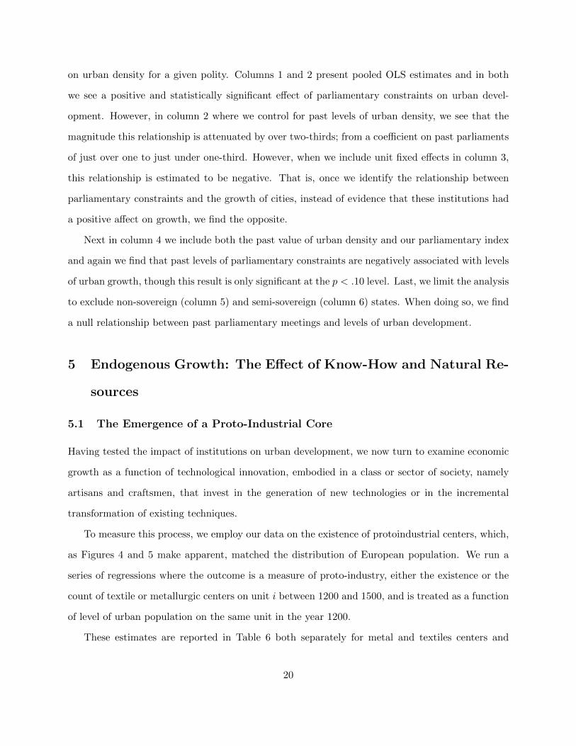
on urban density for a given polity. Columns 1 and 2 present pooled OLS estimates and in both

we see a positive and statistically significant effect of parliamentary constraints on urban devel-

opment. However, in column 2 where we control for past levels of urban density, we see that the

magnitude this relationship is attenuated by over two-thirds; from a coefficient on past parliaments

of just over one to just under one-third. However, when we include unit fixed effects in column 3,

this relationship is estimated to be negative. That is, once we identify the relationship between

parliamentary constraints and the growth of cities, instead of evidence that these institutions had

a positive affect on growth, we find the opposite.

Next in column 4 we include both the past value of urban density and our parliamentary index

and again we find that past levels of parliamentary constraints are negatively associated with levels

of urban growth, though this result is only significant at the p < .10 level. Last, we limit the analysis

to exclude non-sovereign (column 5) and semi-sovereign (column 6) states. When doing so, we find

a null relationship between past parliamentary meetings and levels of urban development.

5 Endogenous Growth: The Effect of Know-How and Natural Re-

sources

5.1 The Emergence of a Proto-Industrial Core

Having tested the impact of institutions on urban development, we now turn to examine economic

growth as a function of technological innovation, embodied in a class or sector of society, namely

artisans and craftsmen, that invest in the generation of new technologies or in the incremental

transformation of existing techniques.

To measure this process, we employ our data on the existence of protoindustrial centers, which,

as Figures 4 and 5 make apparent, matched the distribution of European population. We run a

series of regressions where the outcome is a measure of proto-industry, either the existence or the

count of textile or metallurgic centers on unit i between 1200 and 1500, and is treated as a function

of level of urban population on the same unit in the year 1200.

These estimates are reported in Table 6 both separately for metal and textiles centers and

20

jointly for both types of protoindustry. We report OLS and negative binomial estimates regress

the number of proto-industrial centers in each geographical quadrant on total urban population.

Additionally, we report two-stage least squares estimates with optimal growth temperature again

serving as an instrument of urban population. In all models the estimated effects are positive and

statistically significant. In the appendix we show that all these results are robust to successive

changes in the specification of the independent variable, restricting urban population to be above

towns larger than 5,000, 10,000 and 20,000 inhabitants as well as to the dichotomization of the

independent variable into similarly categorized binary treatments.

There are two results worth emphasizing from Table 6. In the first place, the first-stage results

have a direct substantive causal interpretation in the following sense: they show that in those regions

where agriculture was highly productive, the existence of a food surplus supported the emergence of

towns where a class of individuals could specialize in the development of non-agriculture economic

activities and of new technologies of production. To see this, examine the first stage regression from

the the instrumental variables estimates presented in the lower panel of Table 6 which point to a

substantial negative effect of deviation from the optimal growing temperature of cereals like wheat

on the presence of urban populations in the initial period of 1200: a one degree change in this

measure is predicted to lead to an approximately twenty-five percent decline in urban population.

In the second place, we can interpret the two-stage least squares results as pointing to a causal

effect of initial urban population on the emergence of proto-industrial centers. In terms of their

magnitude, the OLS estimates indicate that a one-hundred percent change in urban population

in the year 1200 would result in .45 of a new industrial center. The 2SLS estimates are larger,

indicating a .85 predicted increase following a 100% change in initial urban population.

If endogenous growth theories (Romer 1990) as well as geographic concentration models (Krug-

man 1991) are correct, urban clusters should have fostered, due some increasing return-to-scale

and positive externalities derived from the agglomeration of individuals, an endogenous process of

economic specialization and technological innovation in which regions with an initial advantage in

their biogeographical endowments experienced ever-faster growth rates. Figure 3 already provided

some evidence that early (more) urbanized areas diverged from rural and semi-rural territories over

21

time. This process, arguably embodied and driven by a proto-industrial sector with a much larger

technological frontier than agriculture, resulted in a faster expansion of population in urban settings

than in semi-urban or rural regions.

To asses the relationship of proto-industrial centers on urbanization (independently of the effect

itself of past urbanization), in Table 7 we regress the urban population (in 1500 and 1800) on

late-medieval textile and iron production centers in existence before 1200 after controlling for prior

urbanization. The top panel in Table 7 presents OLS regressions of the log of urban population in

1800 on the number of proto-industrial center in a particular unit, controlling for urban population

in 1200. The second panel gives results from the same set of regressions treating urban population

in 1500 as the dependent variable.

Disaggregating the effect by type of proto-industrial center, we see that alone textile centers

are not correlated in a statistically significant way with future development. In contrast, there

is a statistically robust relationship between the existence of iron production centers and future

urban development - even after conditioning on past levels of city-size. Considering the effect of

both types of pro industrial activity together we arrive at a similar result as when we consider Iron

alone.

In both logs and levels the addition of a single center of proto-industrial activity is estimated to

be slightly more than half of the magnitude associated with past urban development. For example,

the addition of a single industrial center before 1500 is estimated to yield a 33% and 39% increase

in urban density in 1800 and 1500, respectively. In comparison, the effect of a one-hundred percent

change in urban population in 1200 is predicted to yield a 62 and 66 % change in the same periods.

5.2 Coal

In addition (or independently) of a proto-industrial base, easy access to cheap and abundant energy

sources (coal) has been seen as a crucial condition behind the growth of Europe and, particularly,

the location of the industrial revolution (Landes 19??, Pomeranz 2002). To test this hypothesis,

following Findlay and O’Rourke (2014) we digitized the Les Houillres Europeannes map from Chatel

and Dollfus (1931), which records the location of 124 major nineteenth century coal fields in Europe,

22

and measure the distance for each of our units - either arbitrary grid squares or regions - to the

closest coal field. We are interested in the relationship between access to coal and levels of urban

development in 1800, incomes in the nineteenth century, and, finally, incomes in the twenty-first

century.

To begin, we explore the relationship between access to coal and urban development in 1800 by

estimating a model of the following form

µi,t = α+ β1µi,t−1 + β2Di + β3Di × µi,t−1 + εi (3)

Where µi,t is the logged urban population of quadrant i in the year 1800,µi,t−1 is logged urban

population in the same quadrant in an earlier period - either 1500 or 1700 - and Di is the logged

distance of quadrant i to the nearest coal field. Again, εi is a mean zero random disturbance. The

parameter β1 tells us the direct effect of past urban density, β2 the direct effect of distance to coal,

and β3 the effect of urban density as it varies by distance to coal. The marginal effect of distance

to coal is given by β2 + β3µi,t−1.

Estimates of these effects are given in Table 8. In models where we exclude the interaction term

(Columns 1 and 3) both the effect of past urban density and distance to coal are significant and in

the expected direction. However, the effect of urban population is substantively larger than that

associated with distance to coal. In both models 1 & 3 a one hundred percent change in distance to

coal is estimated to reduce urban population in 1800 by 26% whereas the effect of a one hundred

percent change of in urban population in 1500 and 1700 are expected to produce a 73 and 81 %

change, respectively. In models 2 and 4 of Table 8 we interact past values of urban population with

the distance to the nearest coal field. We see that distance to coal has a negative affect on urban

density but that this effect is declining in past levels of urban agglomeration.

Next, we look at the effect of coal on regional incomes in the nineteenth century. Models 1 and

5 in Table 9 regress regional income in 1870 and 1900 on both distance to coal and urban density in

1800. Here we find evidence that access to coal had an effect on incomes. A one hundred percent

change in urban density is predated to increase income in 1870 by 382 dollars and in 1900 by 542

dollars. Similarly, a one hundred percent change in the minimum distance to coal yields a predicted

23

decline in income of 421 dollars in 1870 and 499 dollar in 1900. Interacting coal and urban density

in 1800 (Columns 2 and 6 of Table 6 ) we obtain similar results. Figure 6 gives the marginal effect of

distance to coal across the interquartile range of urban density in 1800. We see that while incomes

are decreasing in distance to coal they are similarly increasing increasing in past levels of urban

agglomeration. Moreover, when we include country fixed effects so that identification is coming

from within country variation (columns 3 &4 and 5 & 6) the effect of distance to coal becomes

statistically indistinguishable from zero. In contrast, our estimates of the relationship between

urban density in 1800 and per capita incomes in 1870 and 1900 increase in magnitude and remain

statistically significant.

Lastly, we conduct the same analysis now looking at incomes in 2008. These results are presented

in the lower panel of Table 6. In the first four columns we include data from all NUTS-2 regions

and in the last four columns we only include regions from countries for which we have the data on

nineteenth century incomes. In the models where we do not include country fixed effects (1 & 2

and 5 & 6) the relationship between distance to coal in the nineteenth century and income in 2008

is positive and statistically significant. In contrast to the nineteenth century, however, incomes

in regions farther from where coal was mined are higher. Though, when we include country fixed

effects the relationship between access to coal and income per capita in the twenty-first century

becomes statistically insignificant. In contrast, the relationship between past urban density and

incomes remains. In each specification the estimated effect of urban density on incomes in 2008 is

positive. In only one model (Column 5 in the lower panel of of Table 6) where we only examine

Western European countries and do not include country fixed effects this estimate is statistically

insignificant at conventional levels. However, in every other model the estimated effect of a one-

hundred percent change in urban density in 1800 on income in 2008 ranges from 2928 to 5269

dollars and is statistically significant at conventional levels.

In all, we find evidence that while access to coal may have had an impact on incomes in

the nineteenth century, by the twentieth century this correlation disappeared. Moreover, by the

twentieth century past access to coal had a negative correlation with income; evidence of a long

term resource curse. However, past urban agglomeration has a persistent relationship with income

24

both through the nineteenth and twenty-first centuries.

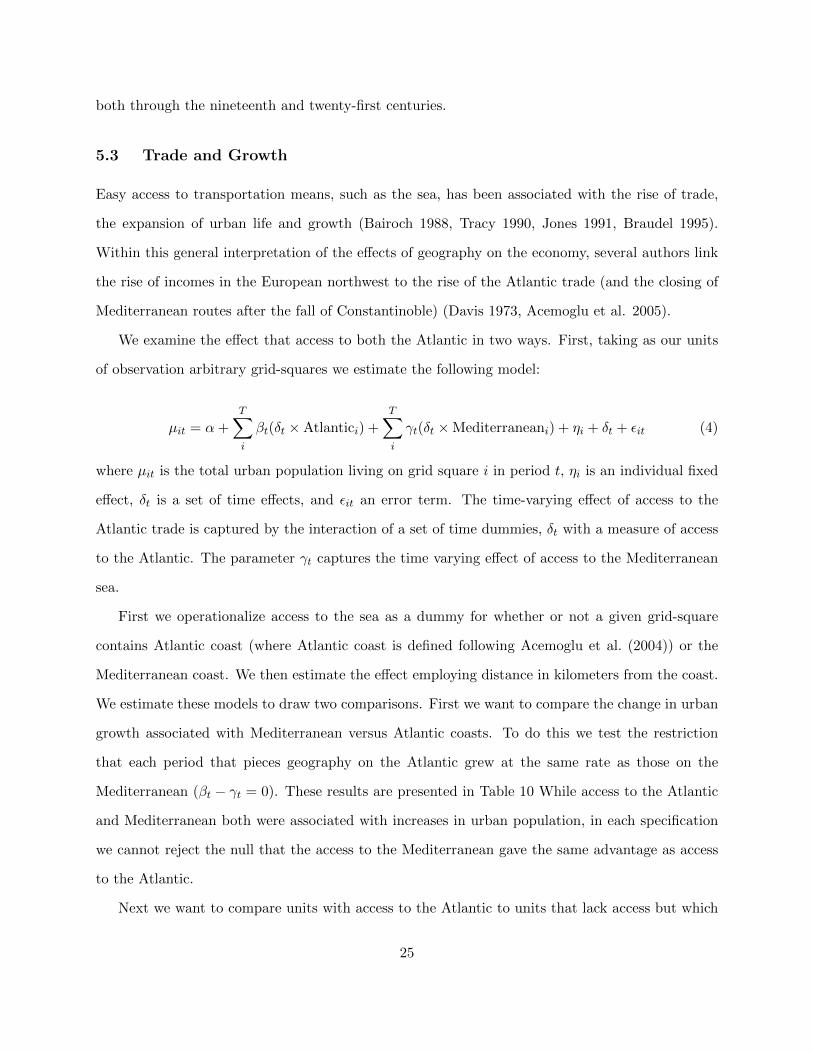
5.3 Trade and Growth

Easy access to transportation means, such as the sea, has been associated with the rise of trade,

the expansion of urban life and growth (Bairoch 1988, Tracy 1990, Jones 1991, Braudel 1995).

Within this general interpretation of the effects of geography on the economy, several authors link

the rise of incomes in the European northwest to the rise of the Atlantic trade (and the closing of

Mediterranean routes after the fall of Constantinoble) (Davis 1973, Acemoglu et al. 2005).

We examine the effect that access to both the Atlantic in two ways. First, taking as our units

of observation arbitrary grid-squares we estimate the following model:

µit = α+T∑i

βt(δt ×Atlantici) +T∑i

γt(δt ×Mediterraneani) + ηi + δt + εit (4)

where µit is the total urban population living on grid square i in period t, ηi is an individual fixed

effect, δt is a set of time effects, and εit an error term. The time-varying effect of access to the

Atlantic trade is captured by the interaction of a set of time dummies, δt with a measure of access

to the Atlantic. The parameter γt captures the time varying effect of access to the Mediterranean

sea.

First we operationalize access to the sea as a dummy for whether or not a given grid-square

contains Atlantic coast (where Atlantic coast is defined following Acemoglu et al. (2004)) or the

Mediterranean coast. We then estimate the effect employing distance in kilometers from the coast.

We estimate these models to draw two comparisons. First we want to compare the change in urban

growth associated with Mediterranean versus Atlantic coasts. To do this we test the restriction

that each period that pieces geography on the Atlantic grew at the same rate as those on the

Mediterranean (βt − γt = 0). These results are presented in Table 10 While access to the Atlantic

and Mediterranean both were associated with increases in urban population, in each specification

we cannot reject the null that the access to the Mediterranean gave the same advantage as access

to the Atlantic.

Next we want to compare units with access to the Atlantic to units that lack access but which

25

were equally urbanized in the previous period. To do this we again estimate a lagged dependent

variable model and continue to allow the effect of access to the Atlantic to vary by period. In these

specifications, once we condition on past values of urban development the relationship between

access to the Atlantic changes. When we use the dichotomous measure of access this relationship

either becomes statistically insignificant (years 1400-1700) or negative (1300). Only in 1800 is this

dichotomous measure of access to the Atlantic positive and statistically significant. When we run

the same model, now using distance to the Atlantic as our measure of access, we find that after

controlling for past levels of urban population pieces of geography closer to the Atlantic were, on

average, less developed than those far away.

5.4 Trade & Parliaments

It may be the case that the combination of constraining political institutions, e.g. parliaments,

and access to the Atlantic trade caused the observed divergence between Western and Eastern

Europe after 1500. Here we directly replicate and then challenge Acemoglu et al. (2004)’s main

finding. Because we have at the level of the political unit time-varying measures of parliamentary

constraints - which they measure only in 1415 - as well as access to the Atlantic - which they

capture as time-invariant fixed features, we are able to improve upon their analysis. We exploit

both of these features of our data to show 1.) The the total effect of access to the Atlantic is

indistinguishable from zero across time periods and 2.) there is no interactive relationship between

access to the Atlantic and parliamentary constraints.

To begin, we follow Acemoglu et al. (2004) in estimating the following baseline model:

µit = αi +

T∑t≥1500

β1t × δt ×Atlantici + β2t × δt ×Atlantici × P-Indexit−1

+T∑

t≥1500γt × δt ×W. Europei + δt + θ × P-Indexit−1 + εit

(5)

Where β1t captures the effect off access to the Atlantic in period t, β2t captures how this effect

varies with the frequency of parliamentary constraints, θ captures the direct effect of parliamentary

constraints, and δt are a set of time dummies. As in Acemoglu et al. (2004) we estimate these

26

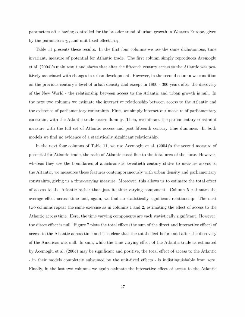
parameters after having controlled for the broader trend of urban growth in Western Europe, given

by the parameters γt, and unit fixed effects, αi.

Table 11 presents these results. In the first four columns we use the same dichotomous, time

invariant, measure of potential for Atlantic trade. The first column simply reproduces Acemoglu

et al. (2004)’s main result and shows that after the fifteenth century access to the Atlantic was pos-

itively associated with changes in urban development. However, in the second column we condition

on the previous century’s level of urban density and except in 1800 - 300 years after the discovery

of the New World - the relationship between access to the Atlantic and urban growth is null. In

the next two columns we estimate the interactive relationship between access to the Atlantic and

the existence of parliamentary constraints. First, we simply interact our measure of parliamentary

constraint with the Atlantic trade access dummy. Then, we interact the parliamentary constraint

measure with the full set of Atlantic access and post fifteenth century time dummies. In both

models we find no evidence of a statistically significant relationship.

In the next four columns of Table 11, we use Acemoglu et al. (2004)’s the second measure of

potential for Atlantic trade, the ratio of Atlantic coast-line to the total area of the state. However,

whereas they use the boundaries of anachronistic twentieth century states to measure access to

the Altantic, we measures these features contemporaneously with urban density and parliamentary

constraints, giving us a time-varying measure. Moreover, this allows us to estimate the total effect

of access to the Atlantic rather than just its time varying component. Column 5 estimates the

average effect across time and, again, we find no statistically significant relationship. The next

two columns repeat the same exercise as in columns 1 and 2, estimating the effect of access to the

Atlantic across time. Here, the time varying components are each statistically significant. However,

the direct effect is null. Figure 7 plots the total effect (the sum of the direct and interactive effect) of

access to the Atlantic across time and it is clear that the total effect before and after the discovery

of the Americas was null. In sum, while the time varying effect of the Atlantic trade as estimated

by Acemoglu et al. (2004) may be significant and positive, the total effect of access to the Atlantic

- in their models completely subsumed by the unit-fixed effects - is indistinguishable from zero.

Finally, in the last two columns we again estimate the interactive effect of access to the Atlantic

27

and parliaments and, as before, find no significant relationship.

6 Interpretation

Around the year 1,000 Europe was an economic and political backwater. The last Carolingian

attempt at unifying the continent had collapsed not long ago, leaving a myriad of small political

units. The economy was strictly agrarian and organized in local, segmented markets. Urban centers

were small and far apart from each other. The biggest town in France at that time, Laon, had 25,000

inhabitants. Around 25,000 people lived in London and 35,000 in Rome. The largest cities lay in

the continental periphery, under either Arab or Byzantine control: Cordova with 468,000 people,

Palermo with 350,000 and Constantinople between 300,000 and half a million persons. Europe was

mired in poverty – the average daily income ranged between $1 and $2 (in dollars of 1990). Yet five

hundred years later, however, Italian per capita income had risen to around $1, 100 or $3.5 a day.

By 1850 some areas of Europe boasted annual per capita income close to $2, 500. The question is

why this happened.

Employing geographic, economic and institutional data that cover 700 years of history we show

that the long-run process of European economic development was related to the formation and

expansion of urban clusters across the continent – especially in the European north-south corridor

that runs from southern England through the Low Countries, the Rhine and Switzerland to northern

and central Italy. Cities emerged in highly productive lands with a substantial cereal surplus,

which could sustain a growing non-farming population that joined in urban agglomerations and

that specialized in a variety of artisanal and proto-industrial activities.

The emergence of these urban clusters acted as an endogenous growth engine. A very sizable

fraction of European towns were agglomerations of traders and artisans. Italian cities were ini-

tially corporations based on the free associations of particular guilds (Weber 1968, Najemy 2006).

Flemish towns, which emerged as small entrepreneurs and production centers supplying their im-

mediate hinterland, eventually asserted their sovereignty over their initial ecclesiastical or feudal

lords (Pirenne 1969). This type of economic and social structure favored economic specialization

and fostered a process of capital accumulation and technological innovation. As shown in the pa-

28

per, urban life in Europe was characterized by very strong historical continuities. The correlation

coefficient between urban populations in 1200 and 1800 is over 0.6 and the level of urbanization

in a given century was a strong predictor of urbanization at subsequent periods. In line with a

growth model with increasing returns to scale and positive intra-sectoral externalities, urban growth

exhibited a divergent pattern across the continent. Those cities that were relatively larger at the

beginning of the period kept adding population at a faster rate than smaller towns such that, by

the end of modern era, Europe had a highly urbanized core extending from Barcelona-Lyon-Naples

in the south to Liverpool-Manchester in the northwest and Hamburg-Dresden-Prague in the east

and much lower urban densities in its western and eastern peripheries.

Parliamentary institutions (acting as a control mechanism of the executive) followed the expan-

sion of urban life. But they played a small independent role in fostering economic growth across

the continent. After peaking in the late fifteenth century, a period which has been identified by

the historical literature as the era of estate representation (Strayer 1973), their power decline with

the intensification of war competition and the consolidation of France and Spain as continental

hegemons, those institutions weakened across the continent, particularly in Italy. They only re-

mained in place, if at all, in the most proto-capitalist enclaves of modern Europe, where a wealthy

urban class had the means to oppose absolutism. Dutch cities joined in a military league and then

a republic that eventually defeated Spain. Likewise, in England the parliamentary forces and the

pro-trade party won over the royal forces in 1640 and again in 1688. As Pincus (2009) writes in his

landmark study of the Glorious Revolution, England in the second half of the seventeenth century

was rapidly becoming a modern society with a booming economy, growing cities and expanding

trade. The opponents of James II looked to the Dutch Republic rather than to the French monar-

chy for political inspiration (Pincus 2009: 7-8), supported the principles of religious toleration

and limited government, rejected James II’s political-economic program based on land interests at

home and territorial acquisition abroad and embraced urban culture, manufacturing and economic

imperialism - understood as - commercial hegemony (ibid, 484).

This wealth had its roots in the artisanal and proto-industrial sectors of European urban clusters.

As shown in the paper, independently of the initial size of a town, having a textile or metal

29

production center in the 14th and 15th centuries had a powerful effect on urbanization throughout

the modern period up until 1800. The effect of these sectors was arguably reinforced by proximity

to energy sources and by easy access to cheap means of transportation. In turn, the presence of an

artisanal class, that is, of a group of people that embodied and carried over a certain production

know-how, had important implications for the modern industrial breakthrough. European artisans

were the only individuals who had the kind of “useful’ or technical knowledge (or, in the terms of

Mokyr (2004) the λ-knowledge) needed to take advantage of the new general knowledge generated by

the scientific revolution of the 17th and the 18th centuries and to apply the latter to the production

process. In other words, knowledge of the principles of Newtonian physics and Lavoisier’s chemistry

could travel quickly from Lisbon to Moscow and Athens. But their profitable application was only

possible in those areas which had a proto-industrial tradition. Urban life in pre-industrial Europe

predicts cross-regional variation in per capita income in the late nineteenth (and early twenty-first)

century quite strongly.

30

References

S. Abramson. Production, predation, and the origins of the territorial state. Mimeo, 2012.

D. Acemoglu, S. Johnson, and J.A. Robinson. Reversal of fortune: Geography and institutions in the makingof the modern world income distribution. Quarterly Journal of Economics, 117(4):1231–1294, 2002.

D. Acemoglu, S. Johnson, and J.A. Robinson. The rise of europe: Atlantic trade, institutional change andeconomic growth. American Economic Review, 2004.

R.C. Allen. The great divergence in european wages and prices from the middle ages to the first world war.Explorations in Economic History, 38(4):411–447, 2001.

P. Anderson. Lineages of the Absolutist State. Verso Books, 1974.

M. Arellano and S. Bond. Some tests of specification for panel data: Monte carlo evidence and an applicationto employment equations. The Review of Economic Studies, 58(2):277–297, 1991.

M. Arellano and O. Bover. Another look at the instrumental variable estimation of error-components models.Journal of econometrics, 68(1):29–51, 1995.

K. Arrow. Economic welfare and the allocation of resources for invention, 1962.

P. Bairoch and C. Braider. Cities and Economic Development: From the Dawn of History to the Present.University of Chicago Press, 1991.

P. Bairoch, J. Batou, and C. Pierre. Population des villes europeennes de 800 a 1850: banque de donnees etanalyse sommaire des resultats (la). Librairie Droz, 1988.

G. Becker, K. Murphy, and R. Tamura. Economic growth, human capital and population growth. Journalof Political Economy, 98(5):S12–S137, 1990.

R. Blundell and S. Bond. Initial conditions and moment restrictions in dynamic panel data models. Journalof econometrics, 87(1):115–143, 1998.

R. Brenner. The Boom and the Bubble: the US in the World Economy. Verso Books, 2003.

E.M. Carus-Wilson. The Woollen Industry. Cambridge Economic History of Europe. Volume II. CambridgeUniversity Press, 1966.

A. Chanda and L. Putterman. Early starts, reversals and catch-up in the process of economic development*.The Scandinavian Journal of Economics, 109(2):387–413, 2007.

G. Clark. A Farewell to Alms: A Brief History of the World. Princeton University Press, Princeton, 2008.

J.B. De Long and A. Shleifer. Princes and merchants’. Journal of Law and Economics, 36, 1993.

J. De Vries. European Urbanization, 1500-1800. Methuen London, 1984.

J. Diamond. Guns, germs and steel. 1997.

G. Duby, H.B. Clarke, and M.B. Becker. The early growth of the european economy: warriors and peasantsfrom the seventh to the twelfth century. History: Reviews of New Books, 2(8):208–208, 1974.

31

S.L. Engerman and K.L. Sokoloff. Factor endowments, inequality, and paths of development among newworld economics. Technical report, National Bureau of Economic Research, 2002.

F. Fukuyama. The end of history? The National Interest, 1989.

Oded Galor, Omer Moav, and Dietrich Vollrath. Inequality in landownership, the emergence of human-capital promoting institutions, and the great divergence. The Review of economic studies, 76(1):143–179,2009.

M.P. Gutmann. Toward the Modern Economy: Early Industry in Europe, 1500-1800. Temple UniversityPress, 1988.

D.A. Hibbs and O. Olsson. Geography, biogeography, and why some countries are rich and others are poor.Proceedings of the National Academy of Sciences of the United States of America, 101(10):3715, 2004.

A. Inkeles. Making men modern: On the causes and consequences of individual change in six developingcountries. American Journal of Sociology, pages 208–225, 1969.

EL Jones. The european miracle: Environments, economies, and geopolitics in the history of europe andasia, 1981.

PD Jones, M. New, DE Parker, S. Martin, and IG Rigor. Surface air temperature and its changes over thepast 150 years. Reviews of Geophysics, 37(2):173–199, 1999.

M. Kremer. Population growth and technological change: One million bc to 1990. The Quarterly Journal ofEconomics, 108(3):681–716, 1993.

P.R. Krugman. Geography and Trade. The MIT Press, 1991.

S. Kuznets. Toward a Theory of Economic Growth: With Reflections on the Economic Growth of ModernNations. Norton, 1968.

R.S. Lopez. The Commercial Revolution of the Middle Ages, 950-1350. Cambridge Univ Pr, 1976.

A. Maddison. The World Economy: Historical Statistics. Organization for Economic Cooperation andDevelopment, 2003.

M.E. Mann, Z. Zhang, S. Rutherford, R.S. Bradley, M.K. Hughes, D. Shindell, C. Ammann, G. Faluvegi,and F. Ni. Global signatures and dynamical origins of the little ice age and medieval climate anomaly.Science, 326(5957):1256, 2009.

J. Mokyr. Punctuated equilibria and technological progress. The American Economic Review, 80(2):350–354,1990.

J. Mokyr. The Gifts of Athena: Historical Origins of the Knowledge Economy. Princeton Univ Pr, 2004.

D. Nicholas. The growth of the medieval city: From late antiquity to the early fourteenth century, 1997.

D.C. North. Institutions, institutional change and economic performance. 1990.

D.C. North and R.P Thomas. The rise of the western world: A new economic history. 1973.

D.C. North and B.R. Weingast. Constitutions and commitment: The evolution of institutions governingpublic choice in seventeenth-century england. Journal of Economic History, 49(4):803–32, 1989.

D.C. North et al. Structure and Change in Economic History. Norton New York, 1981.

32

M. Olson. Dictatorship, democracy, and development. American Political Science Review, pages 567–576,1993.

M. Olson. Power and Prosperity: Outgrowing Communist and Capitalist Dictatorships. Basic books, 2000.

S.L. Parente and E.C. Prescott. Barriers to technology adoption and development. Journal of PoliticalEconomy, pages 298–321, 1994.

S.L. Parente and E.C. Prescott. Monopoly rights: A barrier to riches. American Economic Review, pages1216–1233, 1999.

K. Pomeranz. The Great Divergence: China, Europe, and the Making of the Modern World Economy.Princeton Univ Pr, 2001.

R.D. Putnam. Making Democracy Work: Civic Traditions in Modern Italy. Princeton Univ Pr, 1993.

L.A. Rivera-Batiz and P.M. Romer. Economic integration and endogenous growth. The Quarterly Journalof Economics, 106(2):531–55, 1991.

P.M. Romer. Why, indeed, in america? theory, history, and the origins of modern economic growth. AmericanEconomic Review, 86(2):202–206, 1996.

J.D. Sachs and A.M. Warner. Fundamental sources of long-run growth. The American Economic Review,87(2):184–188, 1997.

A. Smith. The wealth of nations (1776). New York: Modern Library, page 740, 1937 (1776).

R.M. Solow. A contribution to the theory of economic growth. Quarterly Journal of Economics, 70(1):65–94,1956.

R. Sprandel. Das Eisengewerbe im Mittelalter. A. Hiersemann, 1968.

D. Stasavage. Public debt and the birth of the democratic state: France and Great Britain, 1688-1789.Cambridge Univ Pr, 2003.

D. Stasavage. When Distance Mattered: Geographic Scale and the Development of European RepresentativeAssemblies. American Political Science Review, 2011.

J.R. Strayer. On the Medieval Origins of the Modern State. Princeton Univ Pr, 1973.

Guido Tabellini. Culture and institutions: economic development in the regions of europe. Journal of theEuropean Economic Association, 8(4):677–716, 2010.

C. Tilly. Coercion, capital, and European states, AD 990-1990. Basil Blackwell, 1990. ISBN 155786067X.

J.L. van Zanden, E. Buringh, and M. Bosker. The Rise and Decline of European Parliaments, 1188-1789.2010.

N. Voigtlander and H.J. Voth. Why england? demographic factors, structural change and physical capitalaccumulation during the industrial revolution. Journal of Economic Growth, 11(4):319–361, 2006.

M. Weber. Economy and society (g. roth & c. wittich, eds.). New York: Bedminster, 1968.

33

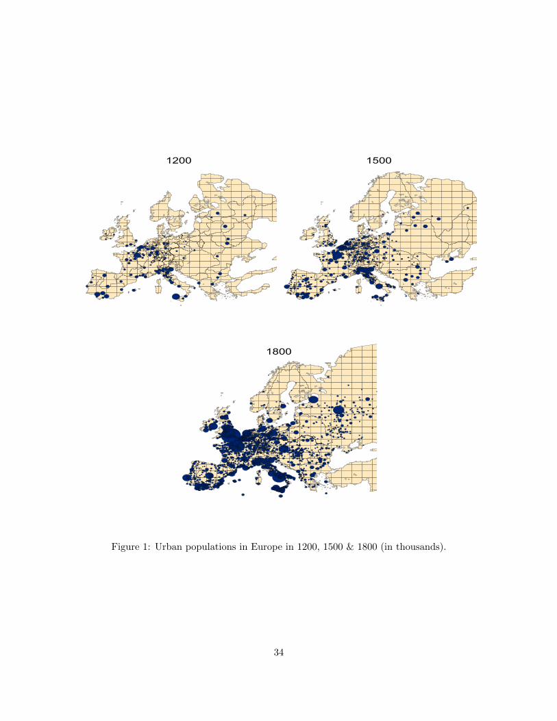
1200 1500

1800

Figure 1: Urban populations in Europe in 1200, 1500 & 1800 (in thousands).

34

●

●

● ●

●

●

●

●

●

●

●

●

●

● ●

●●●●●●●●●●●●●●●●

●

●

●

●

●

●

●●●

●●●●●●●●●●●●●●

●

●

●

●●

●●●

●

●●

●

●●●●●●●●●

●

●

●

●

●

●

●

●●

●●

●●

●

●●●●●●●●●●

●

●

●

●

●

● ●

●●●●●●●●●●●●●●●

●

●

●

● ●

●

●

●●● ●●●●●●●●●●●●

●●●

●

●

●

●

●

●

●

●

●●● ●●●●●●

●

●

●●●●● ●

●

●

●

●

●

●

●●

●●

●●●●●●●●●●●●●●●

●

●●●●●●●●

●

●

●●●●●●●●●●●●●●●

●

●●●●●

●

●

●

●

●

●●●●●●●●●●●●●●●●●●●●

●

●●

●●●●●●●●●●●●●●●●●●●●●●●●●●

●

●●●●●●●●●●●●●●●●●●●●●●●●●●●●●●●●●●●●●●●●●●●●●●●●●●●●●●●●●●●●●●●●●●●●●●●●●●●●●●●●●●●●

●

●●

●

●●●●●●●●●●

●

●●●●

●

●●●●

●

●●●●●●●●●●

●

●●●●●●●●●●●

●

●●●●●●●●

●

●●●●●●●●●●●●●●●●●●

●

●

●

●●

●●●

●

●

●

●

●

●●

●

●●●●●●●●●●

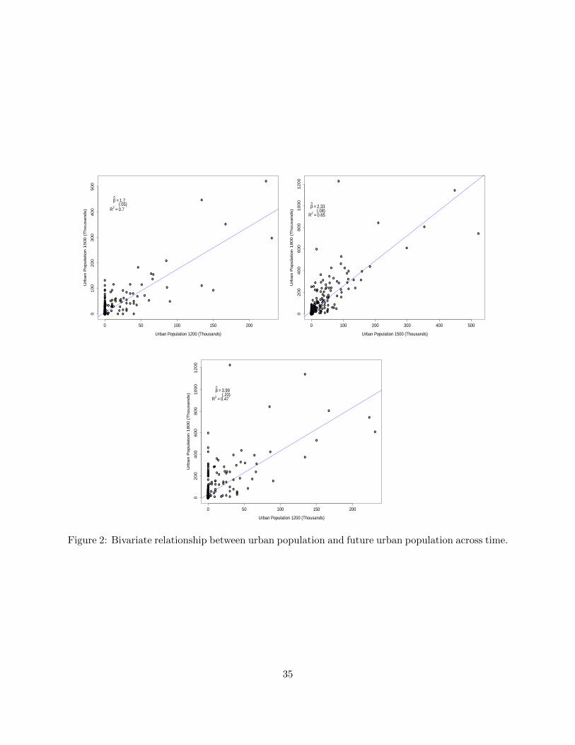
0 50 100 150 200

01

00

20

03

00

40

05

00

Urban Population 1200 (Thousands)

Urb

an

Po

pu

latio

n 1

50

0 (

Th

ou

sa

nd

s)

β = 1.7(.05)

R2 = 0.7

●●

●

●

●

●

●

●

●

●●

●

●●

●

●

●●●●●●●●●

●●

●

●

●●

●

●

●

●

●●

●●

●●●●●●

●

●

●

●

●●●

●

●●●

● ●●●●●

●

●

●

●

●

●

●

●

●

●

●

●●●

●●●●●●

●

●

●

●

●

●

●

●●

●

●●●●●●●

●

●●●●●

●

●

●

●

●

●

●

●●●●●●●●●●●●●●●

●

●

●

●

●

●

●

●

●

●

●

●

●●●

●

●

●●●

●

●

●●●●●●

●

●

●

●

●

●

●

●

●

●●●●

●

●

●●●●●●●●●●

●

●●●●●●

●●● ●

●●

●●

●●

●

●●●●●●●

●

●

●●●●●

●●

●

●●

●●

●●●●●●●●●●●●●

●

●

●

●

●●

●

●

●●●●●

●

●●●●●●●●●●●●●●

●

●●●●●

●

●●●●●●●●●●●●●●●●●●●●●●●●●●●●●●●●●●●●●●●●●●●●●●●●●●●●●●●●●●●●●●●●●●●●●●●●●●●●●●●●●●

●

●●

●

●●●●●●●●●●

●

●●●●

●

●●●●

●

●●●●●●●●●●

●

●●●●●●●●●●

●

●

●●●●●●●●

●●

●●●●●●

●

●●●●●●●●

●

●

●

●

●

●

●●

●

●

●

●

●

●●

●

●●●●●●●

0 100 200 300 400 500

02

00

40

06

00

80

01

00

01

20

0

Urban Population 1500 (Thousands)

Urb

an

Po

pu

latio

n 1

80

0 (

Th

ou

sa

nd

s)

β = 2.33(.08)

R2 = 0.65

●●

●

●

●

●

●

●

●

●●

●

●●

●

●

●●●●●●●●●

●●

●

●

● ●

●

●

●

●

●●

●●

●●●●●●

●

●

●

●

●●●

●

●●●

●●●●●●

●

●

●

●

●

●

●

●

●

●

●

●●●●●●●●●

●

●

●

●

●

●

●

●●

●

●●●●●●●

●

●●●●●

●

●

●

●

●

●

●

●●● ●●●●●●●●●●●●

●

●

●

●

●

●

●

●

●

●

●

●

●●

●

●

●

●●●

●

●

●●●●●●

●

●

●

●

●

●

●

●

●

●●●●

●

●

●●●●●●●●●●

●

●●●●●●●●● ●

●●

●●

●●

●

●●●●●●●●

●

●●●●●

●●

●

●●

●●

●●●●●●●●●●●●●●

●

●

●

●●

●

●

●●●●●

●

●●●●●●●●●●●●●●

●

●●●●●

●

●●●●●●●●●●●●●●●●●●●●●●●●●●●●●●●●●●●●●●●●●●●●●●●●●●●●●●●●●●●●●●●●●●●●●●●●●●●●●●●●●●

●

●●

●

●●●●●●●●●●

●

●●●●

●

●●●●

●

●●●●●●●●●●●

●●●●●●●●●●

●

●

●●●●●●●●

●●

●●●●●●

●

●●●●●●●●

●

●

●

●

●

●

●●

●

●

●

●

●

●●

●

●●●●●●●

0 50 100 150 200

02

00

40

06

00

80

01

00

01

20

0

Urban Population 1200 (Thousands)

Urb

an

Po

pu

latio

n 1

80

0 (

Th

ou

sa

nd

s)

β = 3.99(.20)

R2 = 0.47

Figure 2: Bivariate relationship between urban population and future urban population across time.

35

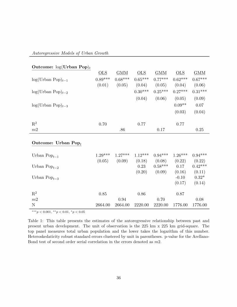
Autoregressive Models of Urban Growth

Outcome: log(Urban Pop)tOLS GMM OLS GMM OLS GMM

log(Urban Pop)t−1 0.89*** 0.68*** 0.65*** 0.77*** 0.62*** 0.67***(0.01) (0.05) (0.04) (0.05) (0.04) (0.06)

log(Urban Pop)t−2 0.30*** 0.25*** 0.27*** 0.31***

(0.04) (0.06) (0.05) (0.09)

log(Urban Pop)t−3 0.09** 0.07

(0.03) (0.04)

R2 0.70 0.77 0.77m2 .86 0.17 0.25

Outcome: Urban Popt

Urban Popt−1 1.29*** 1.27*** 1.12*** 0.94*** 1.26*** 0.94***(0.05) (0.09) (0.18) (0.08) (0.22) (0.22)

Urban Popt−2 0.23 0.58*** 0.17 0.42***(0.20) (0.09) (0.16) (0.11)

Urban Popt−3 -0.10 0.32*(0.17) (0.14)

R2 0.85 0.86 0.87m2 0.94 0.70 0.08N 2664.00 2664.00 2220.00 2220.00 1776.00 1776.00∗∗∗p < 0.001, ∗∗p < 0.01, ∗p < 0.05

Table 1: This table presents the estimates of the autoregressive relationship between past andpresent urban development. The unit of observation is the 225 km x 225 km grid-square. Thetop panel measures total urban population and the lower takes the logarithm of this number.Heteroskedaticity robust standard errors clustered by unit in parentheses. p-value for the Arellano-Bond test of second order serial correlation in the errors denoted as m2.

36

Unit Root Tests

Breitung Test Hadri LM Test(H0: Panels Contain Unit Roots) (H0:All Panels Are Stationary)

log(Urban Pop) Urban Pop log(Urban Pop) Urban Pop

2.47 8.51 22.08∗∗∗ 22.00∗∗∗

(0.99) (0.99) (0.00) (0.00)

Cross-Sectionally Demeaned

9.49 24.33 16.35∗∗∗ 42.56 ∗∗∗

(0.99) (0.99) (0.00) (0.00)

Cross-Sectionally Demeaned & Time Trend

3.80 28.85 4.02∗∗∗ 16.21∗∗∗

(0.99) (0.99) (0.00) (0.00)

∗∗∗p < 0.001, ∗∗p < 0.01, ∗p < 0.05

Table 2: This table presents two types of panel unit-root tests. The null hypothesis of Breitung’stest is that there exist panels with unit root. The null hypothesis in Hadri’s test is that all panelsare stationary. We successively account for common cross-sectional dependence and time-trends.

37

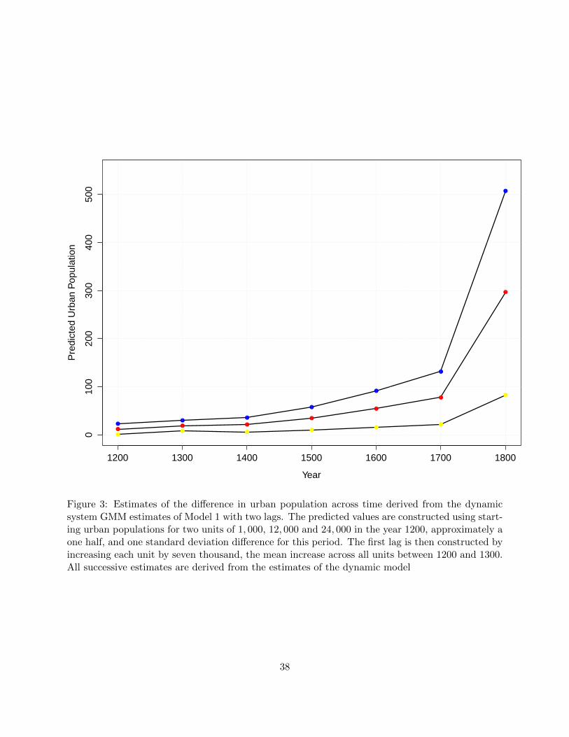
1200 1300 1400 1500 1600 1700 1800

010

020

030

040

050

0

Year

Pre

dict

ed U

rban

Pop

ulat

ion

●●

●

●

●

●

●

●● ●

●

●

●

●

●● ● ●

●●

●

Figure 3: Estimates of the difference in urban population across time derived from the dynamicsystem GMM estimates of Model 1 with two lags. The predicted values are constructed using start-ing urban populations for two units of 1, 000, 12, 000 and 24, 000 in the year 1200, approximately aone half, and one standard deviation difference for this period. The first lag is then constructed byincreasing each unit by seven thousand, the mean increase across all units between 1200 and 1300.All successive estimates are derived from the estimates of the dynamic model

38

The

Rel

atio

nsh

ipB

etw

een

Urb

anD

ensi

tyin

1800

and

Per

Cap

ita

Inco

me

GDP

percapita1870

GDP

percapita1900

GD

Pp

erca

pit

alo

g(G

DP

per

capit

a)G

DP

per

capit

alo

g(G

DP

per

capit

a)G

DP

per

capit

alo

g(G

DP

per

capit

a)G

DP

per

capit

alo

g(G

DP

per

capit

a)

log(U

rban

Den

sity

1800)

400.1

1∗∗∗

0.1

9∗∗∗

329.

61∗∗∗

0.1

5∗∗∗

556.

82∗∗∗

0.1

8∗∗∗

509.

65∗∗∗

0.1

6∗∗∗

(75.

41)

(0.0

3)(5

4.5

8)(0.0

3)(9

8.7

9)(0.0

3)(6

9.6

7)(0.0

2)

Inte

rcep

t39

69.3

0∗∗∗

8.4

4∗∗∗

3365.7

9∗∗∗

8.0

4∗∗∗

5424.1

3∗∗∗

8.7

2∗∗∗

4828.2

7∗∗∗

8.3

7∗∗∗

(329.2

9)(0.1

8)(2

92.6

9)(0.1

7)(3

90.3

5)(0.1

6)(3

59.6

8)(0.1

5)

R2

0.28

0.23

0.80

0.75

0.34

0.25

0.7

90.7

5N

.10

410

410

410

410

610

610

6106

Cou

ntr

yF

ixed

Eff

ects

NN

YY

NN

YY

GD

Pp

er

Cap

ita

in2008

All

Eu

rop

eW

est

ern

Eu

rop

e

log(U

rban

Den

sity

1800)

2583.8

1∗∗∗

0.1

2∗∗∗

3060.2

2∗∗∗

0.1

0∗∗∗

1832.1

20.

04302

9.52∗∗

0.0

7∗∗

(725.5

1)(0.0

2)(8

14.1

4)(0.0

2)(1

037.7

5)(0.0

2)(1

065.0

3)(0.0

2)

Inte

rcep

t15

411.

75∗∗∗

9.5

2∗∗∗

2298

4.0

8∗∗∗

10.0

7∗∗∗

2104

5.1

1∗∗∗

10.0

7∗∗∗

230

84.

13∗∗∗

10.

15∗∗∗

(271

4.5

1)(0.1

1)(3

074.7

2)(0.0

8)(3

822.5

5)(0.0

9)(3

796.8

4)(0.0

9)

R2

0.12

0.11

0.76

0.88

0.10

0.05

0.3

60.3

4N

um

.ob

s.25

425

425

425

416

316

316

3163

Cou

ntr

yF

ixed

Eff

ects

NN

YY

NN

YY

∗∗∗p<

0.001,∗∗

p<

0.01,∗p<

0.05

Table

3:

The

top

panel

of

this

table

des

crib

esth

ere

lati

onsh

ipb

etw

een

urb

an

den

sity

in1800

and

per

capit

ain

com

ein

1870

and

1900,

resp

ecti

vel

y.T

he

low

erof

panel

of

this

table

des

crib

esth

ere

lati

onsh

ipb

etw

een

urb

an

den

sity

in1800

and

per

capit

ain

com

ein

2008.

All

obse

rvati

ons

are

at

the

NU

TS-2

level

.In

the

low

erpanel

the

firs

tfo

ur

colu

mns

use

all

NU

TS-2

regio

ns

for

whic

hth

ere

isin

com

edata

.T

he

last

four

colu

mns

use

only

those

inW

este

rnE

uro

pe.

Het

ereo

sked

act

icty

robust

standard

erro

rscl

ust

ered

by

countr

yare

inpare

nth

eses

.

39

The

Rel

atio

nsh

ipB

etw

een

Urb

anD

ensi

tyan

dP

arli

amen

tary

Con

stra

ints

P-I

nd

ext+

1lo

g(P

-Ind

ex) t+1

P-I

nd

ext+

1lo

g(P

-Ind

ex) t+1

P-I

nd

ext+

1lo

g(P

-Ind

ex) t+1

log(U

rban

Den

sity

)0.

102∗∗∗

0.09

1∗∗∗

0.45

5∗∗∗

0.40

4∗∗∗

0.00

50.

000

0.03

20.

006

0.10

0∗0.

097∗

0.78

7∗∗

0.7

71∗∗

(0.0

1)(0

.01)

(0.0

3)(0

.03)

(0.0

1)(0

.01)

(0.0

5)(0

.04)

(0.0

4)(0

.04)

(0.2

5)(0

.24)

(0.0

1)(0

.01)

(0.0

3)(0

.03)

(0.0

1)(0

.01)

(0.0

5)(0

.05)

(0.0

4)(0

.04)

(0.2

6)(0

.24)

Sov

erei

gnty

Ind

ex0.

342∗∗∗

1.61

5∗∗∗

0.28

3∗∗∗

1.45

8∗∗∗

0.27

2∗∗∗

1.3

71∗∗∗

(0.0

2)(0

.11)

(0.0

4)(0

.16)

(0.0

3)(0

.13)

R2

0.11

80.

222

0.12

40.

231

0.00

00.

152

0.00

10.

168

-0.1

110.

037

-0.2

92-0

.131

First

Sta

ge

|Tem

p−

10.5|

0.71

2∗∗∗

0.71

1∗∗∗

0.71

2∗∗∗

0.7

11∗∗∗

(0.1

2)(0

.11)

(0.1

2)

(0.1

1)

Sov

erei

gnty

Ind

ex0.

113

0.113

(0.0

7)(0

.07)

R2

0.03

60.

038

0.03

60.

038

Fir

stS

tage

F-S

tati

stic

38.2

9719

.785

38.2

9719.7

85

Reg

ion

Eff

ects

YY

YY

Yea

rE

ffec

tsY

YY

Y

Cou

ntr

yE

ffec

tsY

YY

YY

YY

Y

N=

258

T=

2-6

N×

T=

1523

∗∗∗p<

0.001,∗∗

p<

0.01,∗p<

0.05,† p

<0.10

Table

4:T

his

table

pre

sets

the

esti

mate

deff

ect

ofurb

anden

sity

inp

erio

dt

onth

efr

equen

cyw

ith

wh

ich

par

liam

ents

met

inp

erio

ds

tto

t+1.T

he

firs

tei

ght

colu

mn

sgiv

eO

LS

esti

mat

es.T

he

last

four

give

two-

stag

ele

ast

squ

ares

esti

mat

esw

her

ew

eu

secl

imat

icsh

ock

sto

the

pro

pen

sity

togro

wce

real

sas

anin

stru

men

tfo

rurb

anden

sity

.T

he

firs

tst

age

resu

lts

are

pre

sente

din

the

low

erpan

el.

Het

eros

cedast

icit

yro

bust

stand

ard

erro

rsin

par

enth

eses

.

40

!

!

!

!!

!

!!!!!!!!!!!!!!!!!!!!! !

!

!!

!!

!!!!!!!!

!

!

!!!!!!!!

!

!!!!!

!

!!!!!!!!

!!

!

!!

!

!!

!

!!

!!!!!

!!

!

!

!!!

!

!!!!

!! !!! !!!!!

!

!

!!!

!

!!

!!!!!

!!

!!!!! !!!!!!

!!!!!!!!!!!

!

!!

!!! !!

!!

!!!!!!

!!

!

!!!!!!!!!!!!!!!!

!!!!!!

!

!!!!

!!

!

!

!

!

!

!!

!

!

!!!

!!!!!!! !!

!!

!

!!!!!

!

!!

!

!!

!!!

!

!

!!!!!

!! ! !!! !

!! !! !!! !!! !!

!! !! ! !! !! !

!

!!

!

!!!

!!!

!!

!

! !

!

! !!

!!

!

!!

!!

Metallurgic Centers

Figure 4: Iron Production Centers before 1500.

41

##

##

## ##

### #

#

# # ####

###

## #

## ##### ## ## #

# # ### ## ##

# ####### ### #

## ####

## ## # ## # # #### ### ###

##

### ### ####

#

# # ### #

#### ## #

#

## ##### #### ### ##

#### ##

#

# # ## #

##

# # ####

## ## ##

#

#

##

Centers of Textile Production

Figure 5: Textile Centers before 1500.

42

The Marginal Effect of Distance to Coal

1870

GD

PP

C (1

990

GK

$) 3rd Quartile Urban Density

1st Quartile Urban Density

0 2 4 6 8 10

500

1000

1500

2000

2500

3000

3500

1900

0 2 4 6 8 10

500

1000

1500

2000

2500

3000

3500

Distance to Coal (Decimal Degrees)

Figure 6: This figure plots the marginal effect of distance to coal across all observed values holdingacross the interquartile range urban density at the regional level in 1800. The left hand plot givesthese results treating the outcome as income per capita in 1870 and the left hand panel gives it for1900.

43

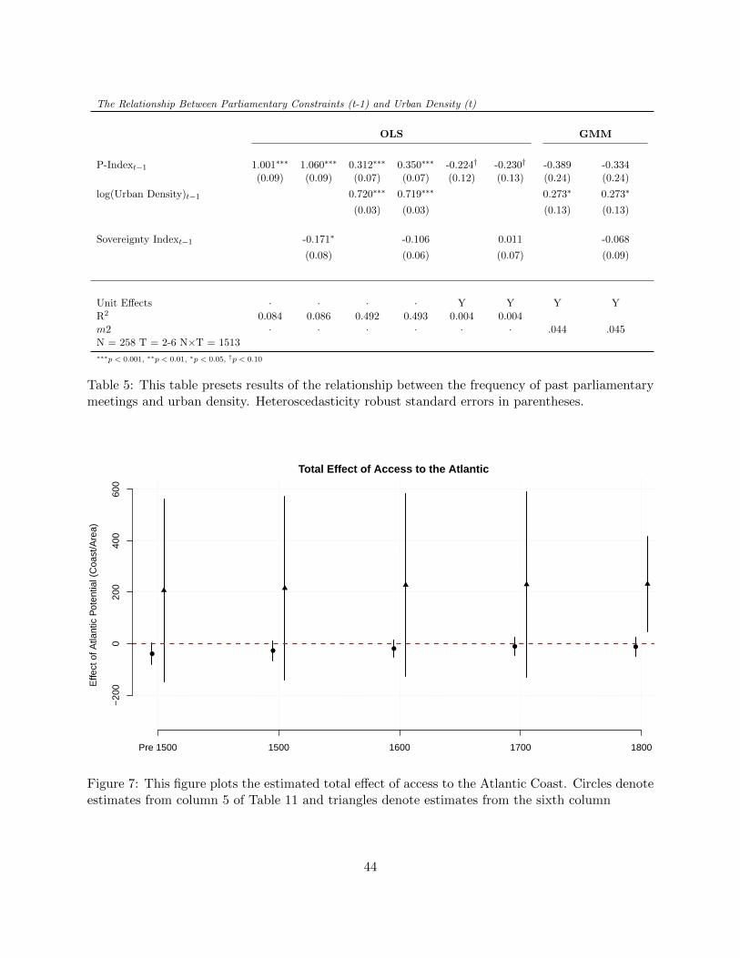
The Relationship Between Parliamentary Constraints (t-1) and Urban Density (t)

OLS GMM

P-Indext−1 1.001∗∗∗ 1.060∗∗∗ 0.312∗∗∗ 0.350∗∗∗ -0.224† -0.230† -0.389 -0.334(0.09) (0.09) (0.07) (0.07) (0.12) (0.13) (0.24) (0.24)

log(Urban Density)t−1 0.720∗∗∗ 0.719∗∗∗ 0.273∗ 0.273∗

(0.03) (0.03) (0.13) (0.13)

Sovereignty Indext−1 -0.171∗ -0.106 0.011 -0.068

(0.08) (0.06) (0.07) (0.09)

Unit Effects · · · · Y Y Y YR2 0.084 0.086 0.492 0.493 0.004 0.004m2 · · · · · · .044 .045N = 258 T = 2-6 N×T = 1513∗∗∗p < 0.001, ∗∗p < 0.01, ∗p < 0.05, †p < 0.10

Table 5: This table presets results of the relationship between the frequency of past parliamentarymeetings and urban density. Heteroscedasticity robust standard errors in parentheses.

●● ● ● ●

Total Effect of Access to the Atlantic

Effe

ct o

f Atla

ntic

Pot

entia

l (C

oast

/Are

a)

Pre 1500 1500 1600 1700 1800

−20

00

200

400

600

Figure 7: This figure plots the estimated total effect of access to the Atlantic Coast. Circles denoteestimates from column 5 of Table 11 and triangles denote estimates from the sixth column

44

Earl

yU

rban

izati

on

an

dT

he

Dev

elopm

ent

of

Pro

toin

du

stry

Iron

Pro

duction

Textile

Pro

duction

Tota

lPro

toindustry

OL

S2S

LS

Neg

ativ

eB

inom

ial

OL

S2S

LS

Neg

ativ

eB

inom

ial

OL

S2S

LS

Neg

ati

veB

inom

ial

Urb

anD

ensi

ty1200

0.0

3∗0.

13∗∗∗

0.0

4∗∗∗

0.0

3∗∗∗

0.07∗∗∗

0.05∗∗∗

0.0

6∗∗

0.2

0∗∗∗

0.05∗∗∗

(0.0

1)(0.0

3)

(0.0

1)(0.0

1)(0.0

2)(0

.00)

(0.0

2)(0.0

4)(0.0

1)

R2

0.11

-0.7

60.

11-0

.76

0.23

-0.8

01/θ

0.06

.28

0.12

log(U

rban

Den

sity

) 1200

0.26∗∗∗

0.54∗∗∗

0.2

2∗∗∗

0.1

9∗∗∗

0.31∗∗∗

.30∗∗∗

0.4

5∗∗∗

0.8

5∗∗∗

0.24∗∗∗

(0.0

5)(0.0

9)

0.0

6(0.0

4)(0.0

6)(0

.04)

(0.0

8)(0.1

2)0.0

6

R2

0.15

-0.0

30.

150.

150.

250.

051/θ

0.07

.72

0.16

First

Sta

ge

Urb

anD

ensi

ty1200

log(U

rban

Den

sity

) 1200

|Tem

p−

10.5|

−1.

07∗∗∗

−0.

25∗∗∗

(0.2

5)(0.0

3)

F-S

tat

onE

xcl

uded

Inst

rum

ent

15.5

241

.00

R2

0.03

0.08

∗∗∗p<

0.001,∗∗

p<

0.01,∗p<

0.05,† p

<0.10

Table

6:T

his

table

pre

sents

esti

mate

sof

the

effec

tof

earl

yurb

and

evel

opm

ent

(in

the

year

1200

)on

the

num

ber

ofp

roto

-ind

ust

rial

cente

rsin

exis

ten

ceon

agi

ven

225

km×

225

km

un

it.

Het

eros

ced

asti

city

rob

ust

stan

dar

der

rors

inpar

enth

eses

.F

irst

stag

ere

sult

sar

epre

sente

din

the

low

erp

anel

.

45

Protoindustry and Later Development

Urban Density log(Urban Density) Urban Density log(Urban Density) Urban Density log(Urban Density)

1800

Textile Center 26.86 0.42(18.08) (0.36)

Iron Production 7.55∗ 0.40∗∗∗

(3.20) (0.07)

Total Protoindustry 9.43∗∗ 0.33∗∗∗

(3.04) (0.07)

Urban Density1200 3.17∗∗∗ 3.74∗∗∗ 3.39∗∗∗

(0.74) (0.66) (0.66)

log(Urban Density1200) 0.68∗∗∗ 0.66∗∗∗ 0.62∗∗∗

(0.06) (0.03) (0.04)

R2 0.52 0.25 0.48 0.27 0.51 0.27N. 444 444 444 444 444 444

1500

Textile Center 8.25∗ 0.45(3.46) (0.34)

Iron Production 2.53∗ 0.48∗∗∗

(1.14) (0.08)

Total Protoindustry 3.04∗∗ 0.39∗∗∗

(0.95) (0.07)

Urban Density1200 1.45∗∗∗ 1.61∗∗∗ 1.50∗∗∗

(0.25) (0.27) (0.26)

log(Urban Density1200) 0.74∗∗∗ 0.70∗∗∗ 0.65∗∗∗

(0.07) (0.05) (0.05)

R2 0.75 0.40 0.72 0.44 0.74 0.44N. 444 444 444 444 444 444

∗∗∗p < 0.001, ∗∗p < 0.01, ∗p < 0.05

Table 7: This table presents results giving the relationship between the existence of proto-industrialcenters on future urban development (in the Years 1500 and 1800, respectively) after conditioningon earlier levels of urban development (in the year 1200). Units are 225 km × 225 km grid-squares.Heteroscedasticity robust standard errors in parentheses.

46

The Relationship Between Distance to Coal and Urban Population in 1800

log(Urban Population1500) 0.73∗∗∗ 0.11(0.04) (0.14)

log(Urban Population1700 ) 0.81∗∗∗ 0.25

(0.03) (0.20)

log(Distance to Coal) −0.26∗∗∗ −0.26∗∗∗ −0.14∗∗∗ −0.22∗∗∗

(0.04) (0.04) (0.03) (0.07)

log(Urban Population1500) × log(Distance to Coal) 0.06∗∗∗

(0.01)

log(Urban Population1800) × log(Distance to Coal) 0.05∗∗

(0.01)

R2 0.56 0.60 0.65 0.67Num. obs. 444 444 444 444

∗∗∗p < 0.001, ∗∗p < 0.01, ∗p < 0.05

Table 8: This table provides estimates of the effects of coal access and urban population on urbanpopulation in 1800. The unit of observation is the 225 km × 225 km grid-square. Heteroskedastictyrobust standard errors clustered by country in parentheses.

47

The Relationship Between Coal, Urban Density, and Incomes

GDP per capita 1870 GDP per capita 1900

log(Urban Density1800) 382.33∗∗∗ 723.08∗∗∗ 328.39∗∗∗ 447.12∗∗∗ 542.52∗∗∗ 1037.39∗∗∗ 508.37∗∗∗ 656.08∗∗∗

(87.46) (103.18) (60.25) (83.64) (116.51) (134.64) (79.06) (124.61)

log(Distance to Coal) −421.86∗∗∗ −2317.00∗∗∗ 10.80 −715.39 −498.81∗∗ −3323.72∗∗∗ 13.12 −907.34

(103.82) (349.59) (123.03) (419.56) (149.94) (475.09) (179.93) (562.59)

log(Urban Density1800) × −361.76∗∗∗ −131.76 −538.71∗∗∗ −166.83

log(Distance to Coal) (65.52) (67.18) (93.12) (88.32)

Country Effects N N Y Y N N Y YR2 0.42 0.55 0.80 0.81 0.45 0.60 0.79 0.80N. 104 104 104 104 106 106 106 106

GDP per Capita in 2008

All Europe Western Europe

log(Urban Density1800) 3117.94∗∗∗ 5269.13∗∗∗ 2986.91∗∗∗ 2927.99∗∗∗ 1948.19 3108.80∗∗ 2934.87∗∗ 2766.28∗∗

(676.53) (798.35) (778.21) (765.11) (1025.28) (1086.59) (1018.05) (937.34)

log(Distance to Coal) 5188.81∗∗∗ 12664.99∗∗∗ 2006.13 1659.78 2731.19 9458.69∗∗∗ 1953.33 672.71

(1371.95) (1995.84) (1450.84) (2086.04) (1439.40) (2679.00) (1782.02) (4011.87)

log(Urban Density1800) × −2590.15∗∗∗ 95.22 −1763.45∗ 311.95

log(Distance to Coal) (530.84) (643.61) (806.82) (1100.01)

Country Effects N N Y Y N N Y YR2 0.19 0.26 0.76 0.76 0.13 0.17 0.37 0.37

Num. obs. 254 254 254 254 163 163 163 163

∗∗∗p < 0.001, ∗∗p < 0.01, ∗p < 0.05

Table 9: This table provides estimates of the effect of urban density in 1800 at the regional levelon incomes in the nineteenth century and twenty first centuries. Heteroskedasticty robust standarderrors clustered by country in parentheses.

48

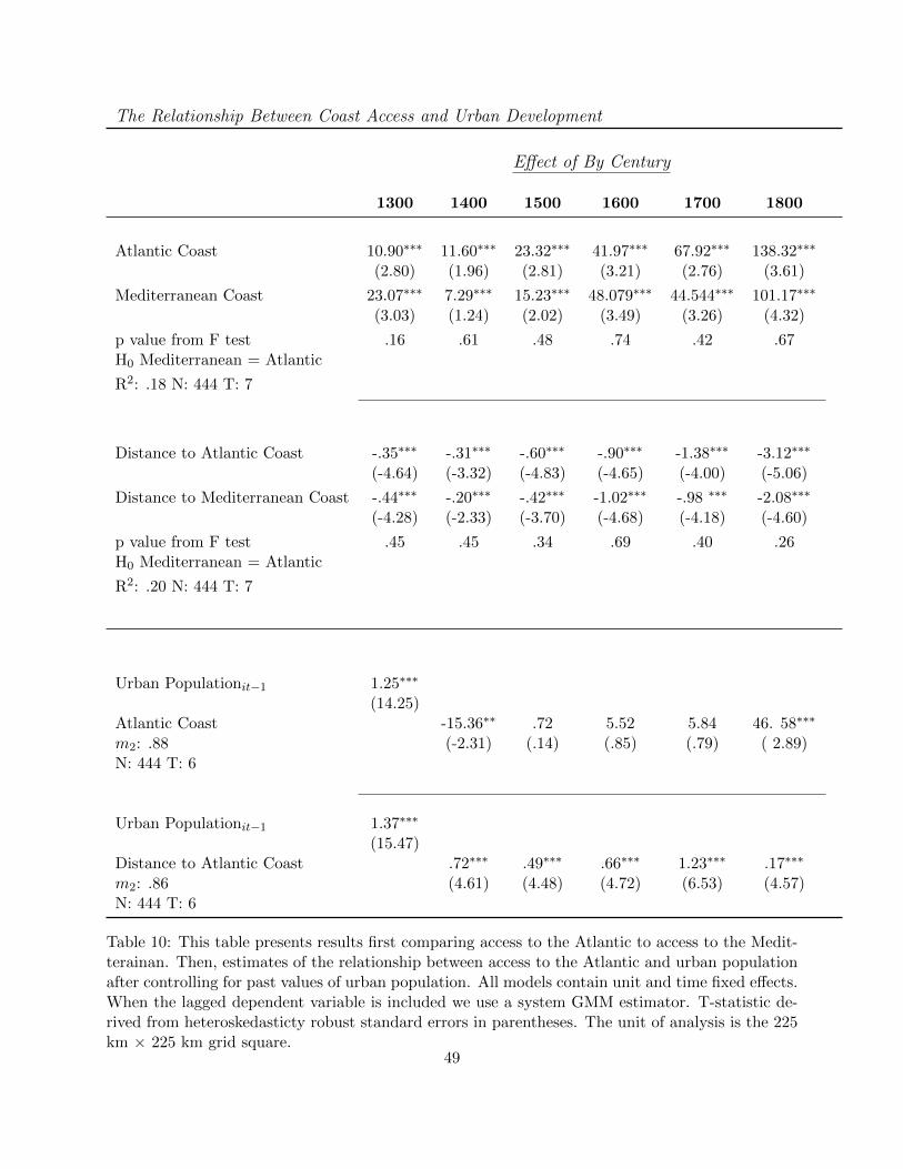
The Relationship Between Coast Access and Urban Development

Effect of By Century

1300 1400 1500 1600 1700 1800

Atlantic Coast 10.90∗∗∗ 11.60∗∗∗ 23.32∗∗∗ 41.97∗∗∗ 67.92∗∗∗ 138.32∗∗∗

(2.80) (1.96) (2.81) (3.21) (2.76) (3.61)

Mediterranean Coast 23.07∗∗∗ 7.29∗∗∗ 15.23∗∗∗ 48.079∗∗∗ 44.544∗∗∗ 101.17∗∗∗

(3.03) (1.24) (2.02) (3.49) (3.26) (4.32)

p value from F test .16 .61 .48 .74 .42 .67H0 Mediterranean = Atlantic

R2: .18 N: 444 T: 7

Distance to Atlantic Coast -.35∗∗∗ -.31∗∗∗ -.60∗∗∗ -.90∗∗∗ -1.38∗∗∗ -3.12∗∗∗

(-4.64) (-3.32) (-4.83) (-4.65) (-4.00) (-5.06)

Distance to Mediterranean Coast -.44∗∗∗ -.20∗∗∗ -.42∗∗∗ -1.02∗∗∗ -.98 ∗∗∗ -2.08∗∗∗

(-4.28) (-2.33) (-3.70) (-4.68) (-4.18) (-4.60)

p value from F test .45 .45 .34 .69 .40 .26H0 Mediterranean = Atlantic

R2: .20 N: 444 T: 7

Urban Populationit−1 1.25∗∗∗

(14.25)Atlantic Coast -15.36∗∗ .72 5.52 5.84 46. 58∗∗∗

m2: .88 (-2.31) (.14) (.85) (.79) ( 2.89)N: 444 T: 6

Urban Populationit−1 1.37∗∗∗

(15.47)Distance to Atlantic Coast .72∗∗∗ .49∗∗∗ .66∗∗∗ 1.23∗∗∗ .17∗∗∗

m2: .86 (4.61) (4.48) (4.72) (6.53) (4.57)N: 444 T: 6

Table 10: This table presents results first comparing access to the Atlantic to access to the Medit-terainan. Then, estimates of the relationship between access to the Atlantic and urban populationafter controlling for past values of urban population. All models contain unit and time fixed effects.When the lagged dependent variable is included we use a system GMM estimator. T-statistic de-rived from heteroskedasticty robust standard errors in parentheses. The unit of analysis is the 225km × 225 km grid square.

49

The Effect of Atlantic Trade and Parliamentary Activity on Urban Density

Atlantic Potential: Dummy Atlantic Potential: Atlantic Coast/Area

Atlantic Potential 13.044 -39.137 223.981 -19.946 -16.024(17.79) (20.94) (179.61) (33.50) (31.58)

log(Urban Density)t−1 0.210† 0.210

(0.12) (0.14)Atlantic Potential × 1500 0.130 0.184 0.111 0.077 12.078** 8.484* 9.153* 11.406†

(0.13) (0.17) (0.12) (0.17) (3.98) (4.08) (3.75) (6.30)

Atlantic Potential × 1600 0.320† 0.344 0.296 0.012 20.004** 21.591*** 17.551** 4.536

(0.18) (0.23) (0.15) (0.16) (7.14) (5.94) (6.26) (8.51)

Atlantic Potential × 1700 0.503* 0.326 0.484* -0.217 28.498** 22.251** 24.505** -10.691

(0.23) (0.26) (0.19) (0.21) (8.73) (6.89) (8.13) (7.75)

Atlantic Potential × 1800 0.517** 0.393* 0.523*** 0.395* 27.171*** 24.981** 24.505*** 18.571*

(0.18) (0.19) (0.15) (0.16) (6.35) (8.77) (5.35) (7.89)

P-Indext−1 -0.181 -0.222 -0.177 -0.220

(0.12) (0.17) (0.12) (0.16)

P-Indext−1 × 1500 0.112 0.114

(0.17) (0.17)

P-Indext−1 × 1600 0.133 0.131

(0.16) (0.16)

P-Indext−1 × 1700 -0.118 -0.115

(0.17) (0.17)

P-Indext−1 × 1800 0.151 0.148

(0.19) (0.19)

Atlantic Potential × P-Indext−1 0.285 0.003 14.318† 7.312

(0.33) (0.38) (8.45) (7.25)

P-Indext−1 × Atlantic Potential × 1500 0.156 -1.799

(0.28) (8.03)

P-Indext−1 × Atlantic Potential × 1600 0.598 22.427

(0.39) (11.86)

P-Indext−1 × Atlantic Potential × 1700 1.314*** 49.234***

(0.39) (9.62)

P-Indext−1 × Atlantic Potential × 1800 0.301 9.361

(0.36) (11.36)

N 1705 1457 1457 1457 1705 1705 1457 1457 1457R2 0.191 0.152 0.157 0.188 0.194 0.155 0.159

m2 · 0.06 · · · · 0.06 · ·

Table 11: This table estimates the relationship between access to the Atlantic and urban develop-ment as well as the interactive effect between Atlantic access and the existence of parliamentaryconstraints on the same outcome. The unit is the polity. Heteroskedasticty robust standard errorsin parentheses. When the lagged dependent variable is included we use the system GMM estimator.

50