EUROPEAN COOPERATION

IN THE FIELD OF SCIENTIFIC

AND TECHNICAL RESEARCH

—————————————————

EURO-COST

—————————————————

IC1004 TD(13)08054

Ghent, Belgium

September 26-27, 2013

SOURCE: Technische Universität Braunschweig (TUBS)

Institute for Communications Technology

Braunschweig, Germany

Universität Stuttgart (UniSTU)

Institute of Communication Networks and Computer Engineering

Stuttgart, Germany

atesio GmbH (ATE)

Berlin, Germany

The IC 1004 Urban Hannover Scenario – 3D Pathloss

Predictions and Realistic Traffic and Mobility Patterns

Dennis M. Rose1, Thomas Jansen

1, Thomas Werthmann

2, Ulrich Türke

3, Thomas Kürner

1

1Technische Universität Braunschweig (TUBS)

Institute for Communications Technology

Schleinitzstraße 22, 38106 Braunschweig, Germany

Phone: +49 531 391 2419

Fax: +49 531 391 5192

Email: rose@ifn.ing.tu-bs.de, jansen@ifn.ing.tu-bs.de, kuerner@ifn.ing.tu-bs.de 2Universität Stuttgart (UniSTU)

Institute of Communication Networks and Computer Engineering

Pfaffenwaldring 47, 70569 Stuttgart, Germany

Email: thomas.werthmann@ikr.uni-stuttgart.de 3atesio GmbH (ATE)

Bundesallee 89, 12161 Berlin, Germany

Email: tuerke@atesio.de

The IC 1004 Urban Hannover Scenario – 3D Pathloss

Predictions and Realistic Traffic and Mobility Patterns

Dennis M. Rose1, Thomas Jansen

1, Thomas Werthmann

2, Ulrich Türke

3, Thomas Kürner

1

1Institute for Communications Technology

Technische Universität Braunschweig

Braunschweig, Germany

{rose, jansen, kuerner}@ifn.ing.tu-bs.de

2Institute of Communication Networks

and Computer Engineering

University of Stuttgart, Germany

thomas.werthmann@ikr.uni-stuttgart.de

3atesio GmbH

Berlin, Germany

tuerke@atesio.de

Abstract— The increasing complexity in today’s mobile networks

enforces the need for more sophisticated and more realistic simu-

lation scenarios. It is a pre-requisite to cope with the effects in

real heterogeneous networks in order to allow the exploitation of

their inherent heterogeneity. This paper describes the first ver-

sion of a common “ready-to-use” simulation environment in the

city of Hannover: A complete LTE network, which has been

modelled for the entire city area. In addition, sophisticated mod-

elling approaches user mobility patterns and for data traffic have

been employed. Furthermore, provisioning a common scenario

ensures the comparability of simulation results, which are based

on this scenario.

Keywords— realistic; scenario; environment; system-level;

pathloss; traffic; mobility;

I. INTRODUCTION

For the development and the evaluation of mechanisms for mobile networks, an adequate system model is an important foundation. Deviating assumptions and implementations of such models render it difficult to compare and reproduce re-search results. Common simulation scenarios are therefore important for the efficiency and quality of research in this area.

Widespread simulation scenarios, like those proposed by the 3GPP, rely on regular geometries and uniform user distri-butions. Thus, they cannot represent the fine shades of real or realistic, complex, heterogeneous environments [1] [2].

In order to provide actual means for the research commu-nity to shift from simple simulation assumptions to a far more reasonable degree of detail – at lowest costs and efforts – this paper aims at providing a common simulation environment in the city of Hannover, Germany. It ensures the comparability of simulation results, which are based on this scenario. Further-more, it allows researchers bringing their focus back to the actual development of smart algorithms instead of re-inventing simulation scenarios again and again.

The idea has been proposed already some time ago in [3] and [4]. The actual realisation of the environment has been accelerated as being pursued in the FP7 project “SEMAFOUR” (2012/09 to 2015/08), which aims at the design and develop-ment of a unified self-management system, that enables the network operators to holistically manage and operate their complex heterogeneous mobile networks [5].

For this purpose, a complete LTE network has been mod-elled for the entire city area of Hannover, as described in Section III of this document. By using real 3D building data, it allows for realistic pathloss predictions and realistic network planning. In addition, sophisticated modelling approaches for macroscopic traffic and individual user mobility have been employed, in order to get a realistic baseline for the simulation of subscribers in the network, as described in Section II. Both sections are partially based on an internal document [6] of the SEMAFOUR project. The described scenario provides the starting point for the development and implementation of the mentioned SON algorithms. They might also be used in context with other advanced network algorithms, which take the timely varying channel conditions of a plethora of different users into account.

Nevertheless, the current simulation scenario is subject to change. We hope that other researchers will use the herein described scenario data and provide us with their feedback on the usability or other needs. Most probably, this process will reveal simulation and/or environmental aspects that need to be optimised in future versions of the simulation scenarios, in order to cope with the special requirements of the individual cases. In order to ease the initial work, the scenario definitions of the “Hannover Scenario” are provided as traces in a com-mon input format, which is specified in Section IV of this document.

This document is organized as follows: Section II describes data sources and simulation models. Section III gives an over-view of the general LTE network in the “Hannover Scenario”. Section IV explains the data format, which is chosen for the provisioning of the data. Section V completes the document with a brief conclusion.

II. ENVIRONMENTAL DATA AND SIMULATION MODELS

In this section, the general data sources for the scenario compilation are introduced. This includes the description of the employed geo data for the generation of the scenarios and the pathloss predictions. Afterwards, an overview of the used mo-bility models is provided, as well as a brief explanation of the process on how to derive pathloss predictions with the chosen propagation models. Last, this section describes the data traffic model.

A. Geo Data

For the generation of the scenarios and the radio propaga-tion pathloss predictions, several data sources have been used, ranging from commercially available data, like 2.5D building information, to GPS road traces available from the Open-StreetMap [7] project.

1) 2.5D Building Information Commercially available 2.5D building information has

been chosen as one source of data for the scenario generation. Here, the shapes of individual buildings are provided as closed 2D polygons, with associated height information for the whole city area of Hannover. The data is used to calculate ray optical outdoor predictions, as described in subsection C.1), and in order to derive the outdoor-to-indoor predictions, as described in subsection C.2).

2) Geographic Information from OpenStreetMap OpenStreetMap (OSM) is an international project founded

in 2004 [8]. It aims on providing a free world map for every-body. Its concept is comparable to the one of Wikipedia: everybody can participate with smaller or larger contributions and everybody is allowed to correct any information that is available. Here, geographic information about many things are collected, e.g.: streets, railroads, waterways, paths, buildings and forests. Nowadays, individual shops, recycling stations and even individual trees or traffic signs are included in the OSM database. Additional information to the shapes in the database is stored in “tags”. A tag is a key-value-pair, represented by strings, which allows storing almost any information – however this makes it hard to automatically digest the database.

Every shape in the OSM database is stored in the decimal format of World Geodetic System 1984 (WGS84) coordinates. In order to transform the contained shapes into input data for the scenario compilation distinct steps have to be done.

First, the information contained in the database needs to be filtered. Depending on the desired content, this can be chal-lenging. Since there are no strong type definitions or enumerations, all tags and value combinations need to be fil-tered on a string comparison base. Once this task has been done, the coordinate system needs to be projected from WGS84 to GK4 (as the Cartesian coordinate system which is officially used in the area of Hannover). In case of vector data, like for building shapes or as the base of SUMO (Simulation of Urban MObility) simulations, this data can be used straight-forward. In case of raster data, like for land-use maps, the shapes have to be prioritised and discretized along a pixel raster.

3) Road Data Road information has been extracted from the OpenStreet-

Map project. Both, raster data and vector data are used. The vector data has been employed to generate user traces for pe-destrian and vehicular users.

Raster data has been derived in order to incorporate the roads in the land-use data. Therefore, a pixel-map with a reso-lution of 10 m along both axes has been computed. Since a street vector does not provide any information about the area it covers, its width is set to 10 m for the time being. This assures that roads are properly represented in a pixel-map with the

resolution of 10 m. A pixel is regarded as being covered by a road, if a street vector is in the vicinity of up to 5 m. 29 differ-ent road types are mentioned in the OSM database for the area of Hannover, but since no further distinction is needed for the land-use data, all of them are treated equally as the land-use class “road”.

4) Land-Use Data Land-use data has been extracted from the OpenStreetMap

project as well. Since shape data is not a practical representa-tion in this context, the vector data needed to be transformed into a pixel-map with a resolution of 10 m along both axes. During the discretization, all shapes are discretized along this raster. If two or more shapes exist on the same point, the shape with the smallest area is chosen, since it is considered to keep the most detailed information. As mentioned, there are differ-ent possibilities to tag shapes and the official documentation describes more than 1000 associations. Therefore, an extensive list of OSM to land-use class mappings has been derived in order to reduce this des-information to a usable degree of in-formation. The result of this filtering and discretization process is 12 different land-use classes (including roads).

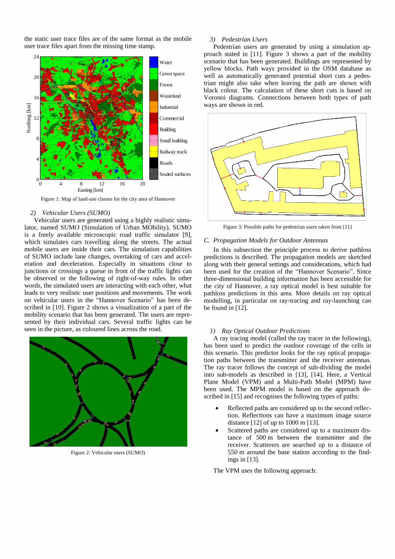
Table 1 presents the respective association of values, land-use classes and arithmetic RGB colour model triplets. Pixels belonging to “Undefined” (meaning that they are not covered by any shapes at all) are assumed to be covered by “Green space”. Thus, the final pixel-map contains values from 2 to 12, only.

Value Land-use class Arithmetic RGB triplet

1 Undefined (0.80, 0.80, 0.80)

2 Sealed surfaces (0.30, 0.30, 0.30)

3 Roads (0.00, 0.00, 0.00)

4 Railway track (1.00, 1.00, 0.00)

5 Small building (1.00, 0.60, 0.78)

6 Building (1.00, 0.00, 0.00)

7 Commercial (0.70, 0.00, 0.00)

8 Industrial (1.00, 0.60, 0.00)

9 Wasteland (0.60, 0.20, 0.00)

10 Forest (0.00, 0.50, 0.00)

11 Green space (0.00, 1.00, 0.00)

12 Water (0.00, 0.00, 1.00)

Table 1: Land-use class encoding incl. RGB colours

In Figure 1, the specified colour triplets have been applied to the map of land-use classes for the city of Hannover.

B. User Mobility Models

One very important aspect in system-level simulations is the change of the environment over time especially in terms of varying spatial traffic. This means, for the simulations of indi-vidual user movements, the users’ positions are generated using different approaches, ranging from static indoor users to highly mobile users, as briefly described in the following subsections.

1) Static Indoor Users The simplest form of user “mobility” is actually where the

position remains constant over time. These static users are useful in order to generate network traffic, which is associated with certain positions but no actual movements. Nevertheless,

the static user trace files are of the same format as the mobile user trace files apart from the missing time stamp.

Figure 1: Map of land-use classes for the city area of Hannover

2) Vehicular Users (SUMO) Vehicular users are generated using a highly realistic simu-

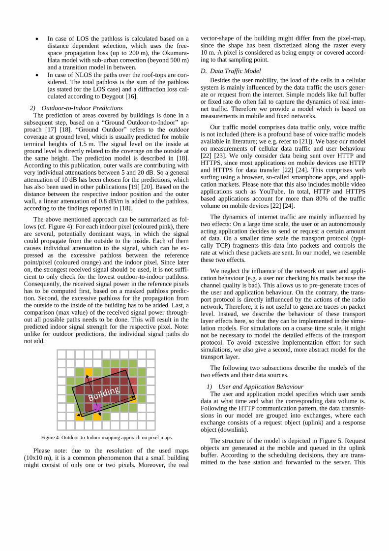
lator, named SUMO (Simulation of Urban MObility). SUMO is a freely available microscopic road traffic simulator [9], which simulates cars travelling along the streets. The actual mobile users are inside their cars. The simulation capabilities of SUMO include lane changes, overtaking of cars and accel-eration and deceleration. Especially in situations close to junctions or crossings a queue in front of the traffic lights can be observed or the following of right-of-way rules. In other words, the simulated users are interacting with each other, what leads to very realistic user positions and movements. The work on vehicular users in the “Hannover Scenario” has been de-scribed in [10]. Figure 2 shows a visualization of a part of the mobility scenario that has been generated. The users are repre-sented by their individual cars. Several traffic lights can be seen in the picture, as coloured lines across the road.

Figure 2: Vehicular users (SUMO)

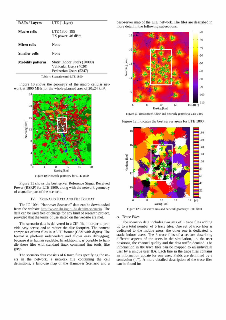
3) Pedestrian Users Pedestrian users are generated by using a simulation ap-

proach stated in [11]. Figure 3 shows a part of the mobility scenario that has been generated. Buildings are represented by yellow blocks. Path ways provided in the OSM database as well as automatically generated potential short cuts a pedes-trian might also take when leaving the path are shown with black colour. The calculation of these short cuts is based on Voronoi diagrams. Connections between both types of path ways are shown in red.

Figure 3: Possible paths for pedestrian users taken from [11]

C. Propagation Models for Outdoor Antennas

In this subsection the principle process to derive pathloss predictions is described. The propagation models are sketched along with their general settings and considerations, which had been used for the creation of the “Hannover Scenario”. Since three-dimensional building information has been accessible for the city of Hannover, a ray optical model is best suitable for pathloss predictions in this area. More details on ray optical modelling, in particular on ray-tracing and ray-launching can be found in [12].

1) Ray Optical Outdoor Predictions A ray tracing model (called the ray tracer in the following),

has been used to predict the outdoor coverage of the cells in this scenario. This predictor looks for the ray optical propaga-tion paths between the transmitter and the receiver antennas. The ray tracer follows the concept of sub-dividing the model into sub-models as described in [13], [14]. Here, a Vertical Plane Model (VPM) and a Multi-Path Model (MPM) have been used. The MPM model is based on the approach de-scribed in [15] and recognises the following types of paths:

Reflected paths are considered up to the second reflec-tion. Reflections can have a maximum image source distance [12] of up to 1000 m [13].

Scattered paths are considered up to a maximum dis-tance of 500 m between the transmitter and the receiver. Scatterers are searched up to a distance of 550 m around the base station according to the find-ings in [13].

The VPM uses the following approach:

Easting [km]

No

rth

ing

[k

m]

0 4 8 12 16 200

4

8

12

16

20

24

Sealed surfaces

Roads

Railway track

Small building

Building

Commercial

Industrial

Wasteland

Forest

Green space

Water

In case of LOS the pathloss is calculated based on a distance dependent selection, which uses the free-space propagation loss (up to 200 m), the Okumura-Hata model with sub-urban correction (beyond 500 m) and a transition model in between.

In case of NLOS the paths over the roof-tops are con-sidered. The total pathloss is the sum of the pathloss (as stated for the LOS case) and a diffraction loss cal-culated according to Deygout [16].

2) Outdoor-to-Indoor Predictions The prediction of areas covered by buildings is done in a

subsequent step, based on a “Ground Outdoor-to-Indoor” ap-proach [17] [18]. “Ground Outdoor” refers to the outdoor coverage at ground level, which is usually predicted for mobile terminal heights of 1.5 m. The signal level on the inside at ground level is directly related to the coverage on the outside at the same height. The prediction model is described in [18]. According to this publication, outer walls are contributing with very individual attenuations between 5 and 20 dB. So a general attenuation of 10 dB has been chosen for the predictions, which has also been used in other publications [19] [20]. Based on the distance between the respective indoor position and the outer wall, a linear attenuation of 0.8 dB/m is added to the pathloss, according to the findings reported in [18].

The above mentioned approach can be summarized as fol-lows (cf. Figure 4): For each indoor pixel (coloured pink), there are several, potentially dominant ways, in which the signal could propagate from the outside to the inside. Each of them causes individual attenuation to the signal, which can be ex-pressed as the excessive pathloss between the reference point/pixel (coloured orange) and the indoor pixel. Since later on, the strongest received signal should be used, it is not suffi-cient to only check for the lowest outdoor-to-indoor pathloss. Consequently, the received signal power in the reference pixels has to be computed first, based on a masked pathloss predic-tion. Second, the excessive pathloss for the propagation from the outside to the inside of the building has to be added. Last, a comparison (max value) of the received signal power through-out all possible paths needs to be done. This will result in the predicted indoor signal strength for the respective pixel. Note: unlike for outdoor predictions, the individual signal paths do not add.

Figure 4: Outdoor-to-Indoor mapping approach on pixel-maps

Please note: due to the resolution of the used maps (10x10 m), it is a common phenomenon that a small building might consist of only one or two pixels. Moreover, the real

vector-shape of the building might differ from the pixel-map, since the shape has been discretized along the raster every 10 m. A pixel is considered as being empty or covered accord-ing to that sampling point.

D. Data Traffic Model

Besides the user mobility, the load of the cells in a cellular system is mainly influenced by the data traffic the users gener-ate or request from the internet. Simple models like full buffer or fixed rate do often fail to capture the dynamics of real inter-net traffic. Therefore we provide a model which is based on measurements in mobile and fixed networks.

Our traffic model comprises data traffic only, voice traffic is not included (there is a profound base of voice traffic models available in literature; we e.g. refer to [21]). We base our model on measurements of cellular data traffic and user behaviour [22] [23]. We only consider data being sent over HTTP and HTTPS, since most applications on mobile devices use HTTP and HTTPS for data transfer [22] [24]. This comprises web surfing using a browser, so-called smartphone apps, and appli-cation markets. Please note that this also includes mobile video applications such as YouTube. In total, HTTP and HTTPS based applications account for more than 80% of the traffic volume on mobile devices [22] [24].

The dynamics of internet traffic are mainly influenced by two effects: On a large time scale, the user or an autonomously acting application decides to send or request a certain amount of data. On a smaller time scale the transport protocol (typi-cally TCP) fragments this data into packets and controls the rate at which these packets are sent. In our model, we resemble these two effects.

We neglect the influence of the network on user and appli-cation behaviour (e.g. a user not checking his mails because the channel quality is bad). This allows us to pre-generate traces of the user and application behaviour. On the contrary, the trans-port protocol is directly influenced by the actions of the radio network. Therefore, it is not useful to generate traces on packet level. Instead, we describe the behaviour of these transport layer effects here, so that they can be implemented in the simu-lation models. For simulations on a coarse time scale, it might not be necessary to model the detailed effects of the transport protocol. To avoid excessive implementation effort for such simulations, we also give a second, more abstract model for the transport layer.

The following two subsections describe the models of the two effects and their data sources.

1) User and Application Behaviour The user and application model specifies which user sends

data at what time and what the corresponding data volume is. Following the HTTP communication pattern, the data transmis-sions in our model are grouped into exchanges, where each exchange consists of a request object (uplink) and a response object (downlink).

The structure of the model is depicted in Figure 5. Request objects are generated at the mobile and queued in the uplink buffer. According to the scheduling decisions, they are trans-mitted to the base station and forwarded to the server. This

generates the corresponding response object and forwards it to the base station. The response is there buffered until it is trans-mitted to the mobile.

Figure 5: Queueing model. Transmissions of different mobiles are independ-

ent, except that they share common radio resources.

The proposed model is based on two distributions of the ob-ject sizes (request and response), a distribution of the number of exchanges per day and user, and a diurnal cell load profile. For the development of our model, we make the following assumptions:

The number of objects sent per user and day is inde-pendent and identically distributed (i.i.d.) and follows a lognormal distribution.

The objects’ sizes are i.i.d.

The time of day the transmission of an object starts is independent from its size and other objects.

Note that we currently neglect dependencies between mul-tiple exchanges, as they are typical in a web session. The modelling of such an interdependency remains for further study.

In the following paragraphs, the components of the data traffic model are derived from data available in the literature.

a) Downlink Object Sizes

The distribution of HTTP response object sizes is heavy-tailed and only slightly differs between fixed and wireless networks [24] [25]. We base our model on the HTTP response size distribution published in [25], which provides a representa-tion of the empirical object size distribution function as a mixture of three lognormal distribution functions. The parame-ters of these distributions are given in Table 2. Figure 6 shows the cumulative distribution function (CDF) of the response object size. It also shows the size-biased response object size distribution function, which illustrates the amount of data a certain object size contributes to the overall downlink traffic volume. While more than 80% of the response objects have less than bytes, they only account for about 20% of the traffic volume.

w

0.55 5.7 0.6

0.4488 8.45 1.2

0.0012 13.05 1.55

Table 2: Parameters of the response object size distribution according to [25].

Here, and denote the mean and the standard deviation of the associated normal distribution, and w denotes the share of object sizes drawn from the

respective distribution.

Figure 6: Object size CDF

Figure 7: Daily per user volume

The capacity of a simulated network depends on many pa-rameters, e.g. technology, bandwidth, carrier aggregation, MIMO modes, and scheduling algorithm. A fixed traffic model would prohibit researchers to evaluate their scenario under load conditions which are realistic for their technologies. Therefore, we introduce a scaling parameter for our object sizes, so that researchers can adapt the load to their needs.

The intuitive way of scaling the object sizes is to multiply the object sizes with a constant factor. However, that leads to a proportional increase of the size of small objects and large objects. Small objects are used for signalling-like applications, e.g. checking whether new mails have arrived, transmitting typed characters in web forms, delivering chat messages etc. It is not reasonable to increase the size of such objects. Instead, we want to increase the size of larger objects (such as applica-tion updates or videos). Hence, we raise the sizes of the objects to the power of a newly introduced parameter . This results in a significantly increased size for large objects, while the size of small objects increases only marginally.

To be able to fill the proposed LTE network scenario to a significant level, we set , which results in an increase of the average object size by factor 20.

b) Uplink Object Sizes

We model the size of uplink objects to follow the same dis-tribution as that of the downlink objects, but apply a different

exponent . We configure such that the uplink data

volume has a relation to the downlink data volume.

We model the size of the request objects to follow the same distribution as the response objects, but scale it by a fixed fac-tor .

[22] observed an average ratio between uplink and downlink of . The authors of [26] observed in a large measurement in 2010, that the factors between uplink and downlink are highly different for different smartphone users. According to their results, about 80% of the users have more downlink traffic than uplink traffic, and the median lies at the ratio ½. As the base for the measurement in [26] is larger, and we assume that the uplink traffic increases due to social web

services, we define . This results in

. Note that the size of the request and the response of each exchange are independent, i.e. it is possible for a single request to be larger than the corresponding response.

c) Number of Exchanges per Day

The number of exchanges per user and day in a cellular network is not known, but some information is available on the overall data volume received per user and day. We thus chose a distribution of the number of exchanges per user and day such that the overall download data volume matches the measured data. Note that the following calculation is based on the objects transmitted in downlink direction only, with the exponent set to 1.

If we consider a total of users, every user transmits exchanges per day, with and . has the dis-tribution function . We denote a response object’s size by , where is the index of the exchange sent by user . The response object size has the distribution function . The downlink data volume generated by user over one day, , is then

From this sum, we get a distribution function of the daily downlink data volume per user. Because the response object size distribution and the distribution of the downlink volume transmitted per user per day are known, we have to construct a function such that

.

The authors of [23] and [22] published data on the data volume generated per user and day. [23] analyzed a one week trace from 2007 of all data traffic in a life nation-wide cellular network. [22] analyzed more recent data collected from 33 Android smartphone users over a period of several months. We extracted the data from both papers and reproduced the corre-sponding cumulative distribution functions in Figure 3. There is a difference of two orders of magnitude between the meas-urements of [23] and [22]. Reasons for this large discrepancy lie in the differences of user populations, devices and pricing schemes of the two studies. The sample in [23] contains many low volume data users, whereas [22] only contains a small set

of moderate to high volume smartphone users. We design our reference scenario to lie on the curve published in [22].

Given the distributions and , we did experi-ments with different distribution functions to find a function such that the distribution of matches . For the input data described here, a lognormal distribution with pa-rameters μ = 8 and σ = 1.4 provides a reasonable fit. Here, μ and σ denote the mean and the standard deviation of the associ-

ated normal distribution. Figure 3 depicts , which is the result of the sum over all objects. Note that, when applying the

exponent , the resulting volume per user per day will differ.

d) Transmission Time

For every object , we draw a random transmission time

from the distribution function , which models the

diurnal network load profile.

The authors of [23] also provide data about the diurnal and weekly load cycles of the network. We do not model the weekly cycle, but use the data on the diurnal load distribution to produce a diurnal load profile for our traffic traces. As the authors only provide six sampling points, we fit a function to the given values. We assume that the same load cycle repeats every day and therefore use a linear combination of sine and cosine functions. Although this fitting function is a bit more complex than a piecewise linear fit, with this function we can easily extend the load profile to multiple days without getting unwanted discontinuities. The function

models the diurnal load profile. Here, is the aggregated network load in gigabytes per hour and t is the time in days. Figure 8 display the diurnal load profile from [23] together with the fitted function . Integration of this function and normalization to a probability sum equal to one results in the following cdf:

Figure 8: Diurnal load profile

For each object which is transmitted in the network, we draw a random number from to determine the time the object arrives at the base station. Under the assumption that every object is immediately transmitted, the resulting load profile corresponds to the one of [23].

2) Transport Layer Behaviour To suit the requirements of different simulation studies, we

envisage to provide two transport layer models with different level-of-detail:

In the bulk transfer model, objects arrive at the mobile or base station as a whole. The respective device can immediately start transmitting the object. The transmission duration depends on the user’s channel quality, the scheduling discipline, the amount of radio resources allocated to the user and maybe other system properties that are specific to the simulation. The request object starts to be transmitted at the time drawn from the distribution function (e.g. the values from the traffic data trace file). After the request has been transmitted in uplink direction, the response object starts to transmit in downlink direction after a delay of , which models the

round-trip time between the base station and the server. Figure 9 depicts the sequence of an exchange.

Figure 9: Sequence of an exchange. The transmission time of the request and

the response depend on the channel quality, resource allocation, and the size

of the request or response, respectively.

The packet-level model includes a detailed TCP model and thus adapts to a user’s throughput in the simulation. Each ex-change is transmitted in a separate TCP connection. After the last bytes of the request arrive at the server, the server starts transmitting the response immediately. This resembles the behaviour of HTTP 1.0 without considering a thinking time at the server.

TCP is a sliding window protocol, where the window size is continuously adapted to the properties of the communication channel. This adaptive behaviour leads to a close interaction between physical and MAC layer mechanisms and the trans-port protocol, which has to be taken into account when studies are conducted on packet-level. Because TCP consists of a set of algorithms to control the behaviour of sender and receiver, it’s behaviour is complex and it is difficult to model it in an ab-stract way. Therefore, we recommend to use a real world TCP implementations in the simulation. One way to integrate the TCP/IP stack of the Linux kernel is to use the Network Simula-tion Cradle (NSC) [27]. Another way is the use of virtual machines as described in [28].

For the results of different studies to be comparable when using a real world TCP/IP stack, we propose the parameters in Table 3, in addition to the parameters of the bulk transfer model.

backhaul capacity unlimited

backhaul delay (one-way) 25 ms

backhaul packet drop probability 0%

uplink queue management backpressure or drop-tail

downlink queue management drop-tail per mobile

uplink queue size max rate · 100ms

downlink queue size (per mobile) max rate · 100ms

maximum transfer unit size 1500 Bytes

congestion control algorithm Cubic

Table 3: Network parameters for packet-level model

III. LTE NETWORK IN THE “HANNOVER SCENARIO”

The current evolution of this scenario consists of a macro cellular network, which covers mainly the suburban and urban regions of the city of Hannover. The area of the “Hannover Scenario”, for which the network is planned, spreads over 20x24 km². In order to minimise border effects in actual simu-lations, an area of only 3x5 km² is considered for simulation purposes and will be used for the collection of user and/or cell statistics. All users mobile and static users reside in the inner area, only. Besides, all pathloss predictions for this scenario are currently made for a height of 1.5 m above ground. In the fu-ture development of this scenario, pathloss prediction layers for different heights are planned. In particular, to cope with the effects of moving users in buildings [29] and indoor deploy-ments of pico and femto cells on different storeys [30].

The base stations used in this scenario are realistic, which means “close to the reality”, but nevertheless artificial. Neither real base station locations nor real base station configurations have been used. So far, a single-layer network for LTE 1800 has been planned, based on publicly available data from the regulatory authority or from publicly reported sites, using an iterative process of planning and optimization. Briefly ex-plained this means, after each step of network geometry planning, the network’s coverage has been predicted and ana-lyzed for coverage holes. Finally, this process resulted in the network presented herein: In total, 195 sectors for the 1800 MHz band have been planned.

Table 4 states the relevant aspects of this scenario and the provided models.

Scenario LTE 1800

Coordinates of the

planned area [m]

E: 00000 … 20000 (20 km)

N: 00000 … 24000 (24 km)

EGK4: 4336000 ... 4356000 (20 km)

NGK4: 5794000 ... 5818000 (24 km)

480 km²

Coordinates of the

scenario area [m]

E: 08500 ... 11500 (3 km)

N: 11000 ... 16000 (5 km)

EGK4: 4344500 ... 4347500 (3 km)

NGK4: 5805000 ... 5810000 (5 km)

15 km²

RATs / Layers LTE (1 layer)

Macro cells LTE 1800: 195

TX power: 46 dBm

Micro cells None

Smaller cells None

Mobility patterns Static Indoor Users (10000)

Vehicular Users (4620)

Pedestrian Users (5247)

Table 4: Scenario card: LTE 1800

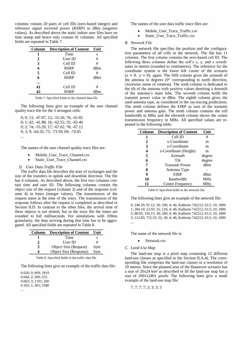
Figure 10 shows the geometry of the macro cellular net-work at 1800 MHz for the whole planned area of 20x24 km².

Figure 10: Network geometry for LTE 1800

Figure 11 shows the best server Reference Signal Received Power (RSRP) for LTE 1800, along with the network geometry of a smaller part of the scenario.

IV. SCENARIO DATA AND FILE FORMAT

The IC 1004 “Hannover Scenario” data can be downloaded from the website http://www.ifn.ing.tu-bs.de/sim-scenario. The data can be used free of charge for any kind of research project, provided that the terms of use stated on the website are met.

The scenario data is delivered in a ZIP file, in order to pro-vide easy access and to reduce the disc footprint. The content comprises of text files in ASCII format (CSV with digits). The format is platform independent and allows easy debugging, because it is human readable. In addition, it is possible to han-dle these files with standard linux command line tools, like grep.

The scenario data consists of 6 trace files specifying the us-ers in the network, a network file containing the cell definitions, a land-use map of the Hannover Scenario and a

best-server map of the LTE network. The files are described in more detail in the following subsections.

Figure 11: Best server RSRP and network geometry: LTE 1800

Figure 12 indicates the best server areas for LTE 1800.

Figure 12: Best server area and network geometry: LTE 1800

A. Trace Files

The scenario data includes two sets of 3 trace files adding up to a total number of 6 trace files. One set of trace files is dedicated to the mobile users, the other one is dedicated to static indoor users. The 3 trace files of a set are describing different aspects of the users in the simulation, i.e. the user positions, the channel quality and the data traffic demand. The information in the trace files can be mapped to an individual user by a unique user IDs. Each line in the trace files contains an information update for one user. Fields are delimited by a semicolon (“;”). A more detailed description of the trace files can be found in:

Easting [km]

No

rth

ing

[k

m]

0 4 8 12 16 200

4

8

12

16

20

24

6 8 10 12 14

10

12

14

16

18

Easting [km]

No

rth

ing

[k

m]

[dBm]-110

-100

-90

-80

-70

-60

-50

-40

-30

-20

6 8 10 12 14

10

12

14

16

18

Easting [km]

Nort

hin

g [

km

]

[#]0

20

40

60

80

100

120

140

160

180

User Position Trace File, described in subsection IV.A.1)

User Channel Quality File, described in subsection IV.A.2)

User Data Traffic File, described in subsection IV.A.3)

This allows to read the files in different parts of a modular-ized simulator.

The scenario incorporates 9867 mobile users and 10000 static indoor users. The mobile users are split among two user types, i.e. vehicular users and pedestrian users. 4620 users of the type vehicular users as described in II.B.2) and 5247 users of the type pedestrian users as described in II.B.3) are included. The trace file data delivers user information updates for 1800 seconds simulation time, i.e. beginning with time stamp 0 sec-onds until time stamp 1799.9. The data traffic corresponds. Figure 13 indicates the spatial distribution of the mobile user traces.

Figure 13: Spatial distribution of the mobile user traces

In the mobile user trace files each line (information update) is tagged with a time stamp starting from zero seconds at the beginning of the file. The lines are sorted by time, which al-lows reading the files sequentially. The mobile users are not active over the complete simulation time and hence user IDs are missing for a time stamp in this case. If a user is active at least a user position and channel quality update is available even if the channel quality did not change. The traffic demand information is only available if additional traffic is added. This data format introduces a certain overhead, as time and user IDs follow a repeating pattern. Nevertheless, each line is self-contained, which allows to easily filter out a set of users or a certain slice in time.

The static user files have no time stamp, i.e. the information does not change over the complete simulation time.

In order to be able to identify the user mobility type the user ID ranges are split among the user types:

Mobility Type User ID Range

Vehicular Users 0 … 4619

Pedestrian Users 10000 … 15246

Static Indoor Users 20000 … 29999

Table 5: User ID ranges for the individual mobility types

For a better readability, this document shows spaces in the file examples between the fields. These spaces are omitted in the actual trace files.

1) User Position Trace File The user position trace file describes the coordinates of the

users over the simulation time. This file has 5 columns. The first two contain the simulation time and user ID. The time resolution is set to 100 ms. The remaining three columns define the user’s x, y, and z coordinates in metres (rounded to centi-metres). The reference for the coordinate system is the lower left corner of the scenario ( ). The values in z direction refer to ground level. Due to the fact that Hannover lies in a flat region no ground level elevation model is taken into account. As described above the static indoor user files have no time stamp and hence only contain 4 columns. All specified fields are repeated in Table 6.

Column Description of Content Unit

1 Time s

2 User ID #

3 x-coordinate m

4 y-coordinate m

5 z-coordinate (height) m

Table 6: Specified fields in the position data file

The following lines give an example of the user position trace file:

0; 0; 256.13; 49.73; 1.5

0; 1; 24.47; 319.62; 1.5

0; 2; 140.57; 161.00; 1.5

0; 3; 196.64; 207.48; 1.5

...

0.1; 0; 256.27; 50.01; 1.5

0.1; 1; 24.47; 319.62; 1.5

0.1; 2; 140.43; 161.33; 1.5

0.1; 3; 196.89; 207.43; 1.5

...

The names of the user position trace files are:

Mobile_User_Trace_Positions.csv

Static_User_Trace_Positions.csv

2) User Channel Quality File The user channel quality trace file describes the channel

quality between a mobile and a cell, for the serving link as well as for interfering links. In order to reduce the file size, weaker links are omitted. Therefore, the channel quality is reported for the 20 strongest cells only, downwards from the strongest to the weaker cells. Hence the file has 42 columns. As described above, the first two columns contain simulation time and user ID. The time resolution is set to 100 ms. The following 40

Easting [km]

Nort

hin

g [

km

]

6 8 10 12 14

10

12

14

16

18

columns contain 20 pairs of cell IDs (zero-based integer) and reference signal received power (RSRP) in dBm (negative values). As described above the static indoor user files have no time stamp and hence only contain 41 columns. All specified fields are repeated in Table 7.

Column Description of Content Unit

1 Time s

2 User ID #

3 Cell ID #

4 RSRP dBm

5 Cell ID #

6 RSRP dBm

…

41 Cell ID #

42 RSRP dBm

Table 7: Specified fields in the channel data file

The following lines give an example of the user channel quality trace file for the 3 strongest cells:

0; 0; 13; -47.87; 12; -55.56; 76; -61.82

0; 1; 42; -41.88; 16; -62.55; 35; -65.40

0; 2; 74; -55.29; 17; -67.02; 78; -67.12

0; 3; 9; -64.35; 75; -73.59; 69; -74.85

...

The names of the user channel quality trace files are:

Mobile_User_Trace_Channel.csv

Static_User_Trace_Channel.csv

3) User Data Traffic File The traffic data file describes the start of exchanges and the

size of the transfers in uplink and downlink direction. The file has 4 columns. As described above, the first two columns con-tain time and user ID. The following columns contain the object size of the request (column 3) and of the response (col-umn 4) in bytes (integer values). The transmission of the request starts at the time of the entry. The transmission of the response follows after the request is completed as described in Section II.D. In contrast to the other files, the arrival time of these objects is not slotted, but in the trace file the times are rounded to full milliseconds. For simulations with 100ms granularity, the data arriving during that time has to be aggre-gated. All specified fields are repeated in Table 8.

Column Description of Content Unit

1 Time s

2 User ID #

3 Object Size (Request) byte

4 Object Size (Response) byte

Table 8: Specified fields in the traffic data file

The following lines give an example of the traffic data file:

0.026; 0; 609; 1819

0.044; 2; 500; 555

0.063; 3; 1191; 260

0.103; 1; 301; 5580

...

The names of the user data traffic trace files are:

Mobile_User_Trace_Traffic.csv

Static_User_Trace_Traffic.csv

B. Network File

The network file specifies the position and the configura-tion parameters of all cells in the network. The file has 11 columns. The first column contains the zero-based cell ID. The following three columns define the cell’s x, y, and z coordi-nates in metres (rounded to centimetres). The reference for the coordinate system is the lower left corner of the scenario ( ), again. The fifth column gives the azimuth of the antenna in degrees (0° corresponding to north direction, clockwise sense of rotation). The sixth column is dedicated to the tilt of the antenna with positive values denoting a downtilt of the antenna’s main lobe. The seventh column holds the transmit power value in dBm. The eighth column gives the used antenna type, as considered in the ray-tracing predictions. The ninth column defines the EIRP as sum of the transmit power and antenna gain. The tenth column contains the cell bandwidth in MHz and the eleventh column shows the centre transmission frequency in MHz. All specified values are re-peated in the following table:

Column Description of Content Unit

1 Cell ID #

2 x-Coordinate m

3 y-Coordinate m

4 z-Coordinate (Height) m

5 Azimuth degree

6 Tilt degree

7 Transmit Power dBm

8 Antenna Type -

9 EIRP dBm

10 Bandwidth MHz

11 Centre Frequency MHz

Table 9: Specified fields in the network file

The following lines give an example of the network file:

0; 148.29; 91.12; 30; 100; 4; 46; Kathrein 742212; 63.5; 10; 1800

1; 284.10; 22.93; 35; 120; 4; 46; Kathrein 742212; 63.5; 10; 1800

2; 88.95; 156.15; 30; 260; 4; 46; Kathrein 742212; 63.5; 10; 1800

3; 112.85; 715.33; 32; 30; 4; 46; Kathrein 742212; 63.5; 10; 1800

...

The name of the network file is:

Network.csv

C. Land-Use Map

The land-use map is a pixel map containing 12 different land-use classes as specified in the Section II.A.4). The corre-sponding file comprises the land-use classes in a resolution of 10 metres. Since the planned area of the Hannover scenario has a size of 20x24 km² as described in III the land-use map has a size of 2001x2401 pixels. The following lines give a small example of the land-use map file:

7; 7; 7; 7; 3; 3; 3; 3

7; 7; 7; 3; 3; 3; 10; 10

7; 7; 10; 10; 3; 3; 6; 6

10; 10; 10; 10; 3; 3; 6; 6

...

The name of the land-use map file is:

Land_Use_Map.csv

D. Best-Server Map

The best-server map is a pixel map containing the cell IDs of the best serving cell for the individual pixel as shown in Figure 11. The corresponding file comprises the best server cell IDs in a resolution of 10 metres. Since the planned area of the Hannover scenario has a size of 20x24 km² as described in III the best-Server map has a size of 2001x2401 pixels. The fol-lowing lines give a small example of the land-use map file:

136; 136; 136; 136; 20; 20; 3; 3

136; 136; 136; 20; 20; 3; 10; 10

136; 136; 9; 9; 20; 204; 204; 6

10; 10; 9; 9; 204; 204; 204; 6

...

The name of the best-server map file is:

Best_Server_Map.csv

V. CONCLUSION AND FUTURE WORK

The presented IC 1004 Urban Hannover Scenario delivers a variety of scenario data in a realistic simulation environment. As motioned earlier we see the currently available data set as a first step towards more complex and modular simulation sce-nario and system simulations. We hope that the utilisation of a freely available, ready-to-use and easy to implement simulation scenario will ease the comparison of simulation results in the future. Feedback from the scientific community on the usability and completeness of the present scenario data will help us to improve the data set for new research activities and is more than welcome.

ACKNOWLEDGEMENT

Parts of this work have been carried out in the FP7 project SEMAFOUR. The authors like to thank all partners involved in the project for their contributions. The authors also like to thank Christian M. Mueller for the contribution of his ideas and valuable discussions.

REFERENCES

[1] D. M. Rose, T. Jansen and T. Kürner, “Modeling of

Femto Cells – Simulation of Interference and Handovers

in LTE Networks,” Proceedings of the IEEE 73rd

Vehicular Technology Conference: VTC2011-Spring,

Budapest, Hungary, May 15th-18th, 2011.

[2] D. M. Rose, J. Baumgarten, T. Jansen and T. Kürner,

“How a Real City Fits into a Hexagonal World,”

Geoinformatik 2012 - Mobilität und Umwelt,

Braunschweig, Germany, March 28th-30th, 2012.

[3] T. Jansen, U. Tuerke, C. M. Mueller and T. Werthmann,

“Proposal of an IC 1004 reference simulation

environment,” European Cooperation in the Field of

Scientific and Technical Research, COST IC1004

TD(11)02050, 2011.

[4] T. Jansen, U. Tuerke, C. M. Mueller and T. Werthmann,

“The IC 1004 Urban Hannover Scenario - 3D Pathloss

Predictions and realistic traffic and mobility patterns,”

European Cooperation in the Field of Scientific and

Technical Research, COST IC1004 TD(12)05059, 2012.

[5] Seventh Framework Programme (FP7), SEMAFOUR

project (Grant agreement no: 316384), “Annex I -

Description of Work”.

[6] D. M. Rose, R. Djapic, H. Hoffmann, L. Jorguseski, I.

Kovacs, D. Laselva, A. Lobinger, K. Trichias, U. Türke

and Y. Wang, “Definition of Reference Scenarios,

Modelling Assumptions and Methodologies (Deliverable

D2.4),” SEMAFOUR (Internal Document), pp. 1-74, July

31, 2013.

[7] OpenStreetMap, “OpenStreetMap,” 2013. [Online].

Available: http://www.openstreetmap.org.

[8] OpenStreetMap, “History of OpenStreetMap,” 2013.

[Online]. Available:

http://wiki.openstreetmap.org/wiki/History_of_OpenStre

etMap.

[9] “SUMO - Simulation of Urban MObility,” [Online].

Available: http://sumo.sourceforge.net/. [Accessed 14

November 2011].

[10] J. Baumgarten, “Repeater - Möglichkeit zur

Verbesserung des Load Balancing in LTE?,”

Diplomarbeit, Technische Universität Braunschweig,

Institut für Nachrichtentechnik, Dipl. 11/026, 2011.

[11] J. Sulak, “Integration eines Fahrradfahrer- und

Fußgänger-Mobilitätsmodells in einen LTE-Simulator,”

Diplomarbeit, Technische Universität Braunschweig,

Institut für Nachrichtentechnik, Dipl. 12/014, 2012.

[12] Y. Lostanlen and T. Kürner, “Ray Tracing Modeling,” in

LTE Advanced and Next Generation Wireless Networks:

Channel Modeling and Propagation, Wiley, 2012, pp.

271-291.

[13] T. Kürner, “A run-time efficient 3D propagation model

for urban areas including vegetation and terrain effects,”

49th IEEE Vehicular Technology Conference, vol. 1, pp.

782 - 786, Jul 1999.

[14] T. Kürner and A. Meier, “Prediction of Outdoor and

Outdoor-to-Indoor Coverage in Urban Areas at 1.8 GHz,”

IEEE Journal on Selected Areas in Communications, Vol.

20, No. 3, pp. 496-506, April 2002.

[15] T. Kürner and M. Schack, “3D-Ray-Tracing embedded

into an integrated simulator for car-to-x-communication,”

URSI International Symposium on Electromagnetic

Theory (EMTS), pp. 880-882, August 2010.

[16] J. Deygout, “Multiple knife-edge diffraction of

microwaves,” IEEE Transactions on Antennas and

Propagation, vol. 14, no. 4, pp. 480 - 489, Jul 1966.

[17] R. Gahleitner and E. Bonek, “Radio wave penetration

into urban buildings in small cells and micro cells,”

Proceedings of the IEEE Vehicular Technology

Conference: VTC1994, pp. 887-891, Budapest,

Stockholm, May 1994.

[18] D. M. Rose and T. Kürner, “Outdoor-to-Indoor

Propagation – Accurate Measuring and Modeling of

Indoor Environments at 900 and 1800 MHz,” 6th

European Conference on Antennas and Propagation,

2012. EuCAP 2012., Prague, Czech Republic, 2012.

[19] H. Okamoto, K. Kitao and S. Ichitsubo, “Outdoor-to-

Indoor Propagation Loss Prediction in 800-MHz to 8-

GHz Band for an Urban Area,” IEEE Transactions on

Vehicular Technology, vol.58, no.3, pp. 1059-1067,

March 2009.

[20] R. Hoppe, G. Wolfle and F. M. Landstorfer,

“Measurement of building penetration loss and

propagation models for radio transmission into

buildings,” 50th IEEE VTC 1999, Vehicular Technology

Conference, 1999. - Fall., vol. 4, pp. 2298-2302, 1999.

[21] P. Orlik and S. Rappaport, “A model for teletraffic

performance and channel holding time characterization in

wireless cellular communication with general session and

dwell time distributions,” IEEE Journal on Selected

Areas in Communications, vol. 16, no. 5, pp. 788-803,

1998.

[22] H. Falaki, D. Lymberopoulos, R. Mahajan, S. Kandula

and D. Estrin, “A first look at traffic on smartphones,”

Internet Measurements Conference (IMC), Melbourne,

Australia, November 2010.

[23] U. Paul, A. Subramanian, M. Buddhikot and S. Das,

“Understanding traffic dynamics in cellular data

networks,” IEEE INFOCOM, p. 882–890, 2011.

[24] G. Maier, F. Schneider and A. Feldmann, “A first look at

mobile handheld device traffic,” 11th International

Conference on Passive and Active Network

Measurement, 2010.

[25] F. Hernandez-Campos, J. Marron, G. Samorodnitsky and

F. Smith, “Variable heavy tails in internet traffic,”

Performance Evaluation, vol. 58, no. 2-3, Nov 2004.

[26] M. Z. Shafiq, L. Ji, A. X. Liu, J. Pang and J. Wang, “A

first look at cellular machine-to-machine traffic: large

scale measurement and characterization,” Proceedings of

the 12th ACM SIGMETRICS/PERFORMANCE joint

international conference on Measurement and Modeling

of Computer Systems, ser. SIGMETRICS’12, p. 65–76,

New York, NY, USA. 2012.

[27] S. Jansen and A. McGregor, “Simulation with real world

network stacks,” Winter Simulation Conference, 2005.

[28] T. Werthmann, M. Kaschub, C. Blankenhorn and C. M.

Mueller, “Approaches for evaluating the application

performance of future mobile networks,” European

Cooperation in the Field of Scientific and Technical

Research, COST IC1004 TD(11)01038, 2011.

[29] D. M. Rose, T. Jansen, S. Hahn and T. Kürner, “Impact

of Realistic Indoor Mobility Modelling in the Context of

Propagation Modelling on the User and Network

Experience,” 2013.

[30] D. M. Rose, T. Jansen and T. Kürner, “Indoor to Outdoor

Propagation – Measuring and Modeling of Femto Cells in

LTE Networks at 800 and 2600 MHz,” IEEE

GLOBECOM Workshops, pp. 203-207, Houston, Texas,

December 5th-9th, 2011.