THE DEVELOPMENT OF THREE-DIMENSIONAL ADJOINT …
163
The Pennsylvania State University The Graduate School Department of Aerospace Engineering THE DEVELOPMENT OF THREE-DIMENSIONAL ADJOINT METHOD FOR FLOW CONTROL WITH BLOWING IN CONVERGENT-DIVERGENT NOZZLE FLOWS A Dissertation in Aerospace Engineering by Nidhi Sikarwar c 2015 Nidhi Sikarwar Submitted in Partial Fulfillment of the Requirements for the Degree of Doctor of Philosophy May 2015
Transcript of THE DEVELOPMENT OF THREE-DIMENSIONAL ADJOINT …

The Pennsylvania State University
The Graduate School
Department of Aerospace Engineering
THE DEVELOPMENT OF THREE-DIMENSIONAL ADJOINT
METHOD FOR FLOW CONTROL WITH BLOWING IN
CONVERGENT-DIVERGENT NOZZLE FLOWS
A Dissertation in
Aerospace Engineering
by
Nidhi Sikarwar
c© 2015 Nidhi Sikarwar
Submitted in Partial Fulfillmentof the Requirements
for the Degree of
Doctor of Philosophy
May 2015

The dissertation of Nidhi Sikarwar was reviewed and approved1 by the following:
Philip J. MorrisProfessor of Aerospace EngineeringDissertation AdviserChair of Committee
D. K. McLaughlinProfessor of Aerospace Engineering
Mark D. MaughmerProfessor of Aerospace Engineering
Daniel C. HaworthProfessor of Mechanical Engineering
George A. LesieutreProfessor of Aerospace EngineeringHead of the Department of Aerospace Engineering
1Signatures on file in the Graduate School.

iii
Abstract
The noise produced by the low bypass ratio turbofan engines used to power fighter air-craft is a problem for communities near military bases and for personnel working in closeproximity to the aircraft. For example, carrier deck personnel are subject to noise expo-sure that can result in Noise-Induced Hearing Loss which in-turn results in over a billiondollars of disability payments by the Veterans Administration. Several methods havebeen proposed to reduce the jet noise at the source. These methods include microjetinjection of air or water downstream of the jet exit, chevrons, and corrugated nozzleinserts. The last method involves the insertion of corrugated seals into the divergingsection of a military-style convergent-divergent jet nozzle (to replace the existing seals).This has been shown to reduce both the broadband shock-associated noise as well as themixing noise in the peak noise radiation direction. However, the original inserts weredesigned to be effective for a take-off condition where the jet is over-expanded. Thenozzle performance would be expected to degrade at other conditions, such as in cruiseat altitude. A new method has been proposed to achieve the same effects as corrugatedseals, but using fluidic inserts. This involves injection of air, at relatively low pressuresand total mass flow rates, into the diverging section of the nozzle. These “fluidic inserts”deflect the flow in the same way as the mechanical inserts. The fluidic inserts representan active control method, since the injectors can be modified or turned off dependingon the jet operating conditions. Noise reductions in the peak noise direction of 5 to 6dB have been achieved and broadband shock-associated noise is effectively suppressed.There are multiple parameters to be considered in the design of the fluidic inserts. Thisincludes the number and location of the injectors and the pressures and mass flow ratesto be used. These could be optimized on an ad hoc basis with multiple experiments ornumerical simulations. Alternatively an inverse design method can be used. An adjointoptimization method can be used to achieve the optimum blowing rate. It is shown thatthe method works for both geometry optimization and active control of the flow in orderto deflect the flow in desirable ways.
An adjoint optimization method is described. It is used to determine the blowing dis-tribution in the diverging section of a convergent-divergent nozzle that gives a desiredpressure distribution in the nozzle. Both the direct and adjoint problems and their asso-ciated boundary conditions are developed. The adjoint method is used to determine theblowing distribution required to minimize the shock strength in the nozzle to achieve a

iv
known target pressure and to achieve close to an ideally expanded flow pressure.
A multi-block structured solver is developed to calculate the flow solution and associatedadjoint variables. Two and three-dimensional calculations are performed for internal andexternal of the nozzle domains. A two step MacCormack scheme based on predictor-corrector technique is was used for some calculations. The four and five stage Runge-Kutta schemes are also used to artificially march in time. A modified Runge-Kuttascheme is used to accelerate the convergence to a steady state. Second order artificialdissipation has been added to stabilize the calculations. The steepest decent methodhas been used for the optimization of the blowing velocity after the gradients of thecost function with respect to the blowing velocity are calculated using adjoint method.Several examples are given of the optimization of blowing using the adjoint method.

v
Table of Contents
List of Tables . . . . . . . . . . . . . . . . . . . . . . . . . . . . . . . . . . . . . . vii
List of Figures . . . . . . . . . . . . . . . . . . . . . . . . . . . . . . . . . . . . . viii
Nomenclature . . . . . . . . . . . . . . . . . . . . . . . . . . . . . . . . . . . . . . xi
Acknowledgments . . . . . . . . . . . . . . . . . . . . . . . . . . . . . . . . . . . xiv
Chapter 1.. Introduction and Background . . . . . . . . . . . . . . . . . . . . . . 11.1. Motivation for Noise Reduction and Available Methods . . . . . . . . 11.2. Fluidic Inserts . . . . . . . . . . . . . . . . . . . . . . . . . . . . . . . 71.3. Use of Adjoint Method . . . . . . . . . . . . . . . . . . . . . . . . . . 141.4. The Adjoint Approach . . . . . . . . . . . . . . . . . . . . . . . . . . 161.5. Passive Control Using Adjoint Method . . . . . . . . . . . . . . . . . 171.6. Thesis outline . . . . . . . . . . . . . . . . . . . . . . . . . . . . . . . 201.7. Original Contribution of the Thesis . . . . . . . . . . . . . . . . . . . 21
Chapter 2.. General Development of the Adjoint Method . . . . . . . . . . . . . 232.1. General Approach . . . . . . . . . . . . . . . . . . . . . . . . . . . . 242.2. Outline of the Design Procedure . . . . . . . . . . . . . . . . . . . . 272.3. Discrete and Continuous Approaches . . . . . . . . . . . . . . . . . . 292.4. Steady and Time Dependent Problems . . . . . . . . . . . . . . . . . 312.5. Summary . . . . . . . . . . . . . . . . . . . . . . . . . . . . . . . . . 32
Chapter 3.. Numerical Method . . . . . . . . . . . . . . . . . . . . . . . . . . . . 343.1. Numerical Schemes . . . . . . . . . . . . . . . . . . . . . . . . . . . . 35
3.1.1. MacCormack Scheme . . . . . . . . . . . . . . . . . . . . . . . 353.1.2. Central Difference Schemes . . . . . . . . . . . . . . . . . . . 373.1.3. Time Marching Schemes . . . . . . . . . . . . . . . . . . . . . 373.1.4. Local Time Stepping . . . . . . . . . . . . . . . . . . . . . . . 41
3.2. Multi-Block Topology . . . . . . . . . . . . . . . . . . . . . . . . . . 433.3. Artificial Dissipation . . . . . . . . . . . . . . . . . . . . . . . . . . . 443.4. Summary . . . . . . . . . . . . . . . . . . . . . . . . . . . . . . . . . 46

vi
Chapter 4.. Direct and Adjoint Characteristics Analysis . . . . . . . . . . . . . . 484.1. Grid singularities . . . . . . . . . . . . . . . . . . . . . . . . . . . . . 484.2. Characteristics and Interface Boundary Conditions for the Direct
Flow Equations . . . . . . . . . . . . . . . . . . . . . . . . . . . . . . 514.3. Adjoint Characteristics and Interface Boundary Conditions . . . . . 524.4. Results . . . . . . . . . . . . . . . . . . . . . . . . . . . . . . . . . . . 544.5. Conclusion . . . . . . . . . . . . . . . . . . . . . . . . . . . . . . . . . 624.6. Summary . . . . . . . . . . . . . . . . . . . . . . . . . . . . . . . . . 62
Chapter 5.. Parameterization of the Control . . . . . . . . . . . . . . . . . . . . . 645.1. The Mathematical Development . . . . . . . . . . . . . . . . . . . . . 655.2. Optimization with Parameterization of Blowing . . . . . . . . . . . . 715.3. Conclusion . . . . . . . . . . . . . . . . . . . . . . . . . . . . . . . . . 775.4. Summary . . . . . . . . . . . . . . . . . . . . . . . . . . . . . . . . . 78
Chapter 6.. Adjoint Control of Nozzle Flow with Surface Blowing . . . . . . . . . 796.1. Introduction . . . . . . . . . . . . . . . . . . . . . . . . . . . . . . . . 796.2. The Mathematical Development with Wall Blowing Control . . . . . 806.3. Boundary Conditions . . . . . . . . . . . . . . . . . . . . . . . . . . . 86
6.3.1. Adjoint Outflow Boundary Condition . . . . . . . . . . . . . 896.3.1.1. Subsonic Outflow . . . . . . . . . . . . . . . . . . . 896.3.1.2. Supersonic outflow . . . . . . . . . . . . . . . . . . . 90
6.3.2. Adjoint Inflow Boundary Condition . . . . . . . . . . . . . . . 916.3.3. Adjoint Slip Wall Boundary Condition . . . . . . . . . . . . . 926.3.4. Sensor Boundary Condition . . . . . . . . . . . . . . . . . . . 936.3.5. Actuator Boundary Condition . . . . . . . . . . . . . . . . . . 94
6.4. The Optimization Procedure . . . . . . . . . . . . . . . . . . . . . . 966.5. Results and Discussion . . . . . . . . . . . . . . . . . . . . . . . . . . 976.6. Two-dimensional Optimization of Blowing . . . . . . . . . . . . . . 97
6.6.1. Example 1 . . . . . . . . . . . . . . . . . . . . . . . . . . . . . 986.6.2. Example 2 . . . . . . . . . . . . . . . . . . . . . . . . . . . . . 1016.6.3. Three-dimensional Optimization of Blowing . . . . . . . . . . 107
6.7. External Flow Calculations . . . . . . . . . . . . . . . . . . . . . . . 1186.8. Conclusion . . . . . . . . . . . . . . . . . . . . . . . . . . . . . . . . . 1246.9. Summary . . . . . . . . . . . . . . . . . . . . . . . . . . . . . . . . . 124
Chapter 7.. Conclusions and Future Work . . . . . . . . . . . . . . . . . . . . . . 126
Appendix A.. The Solver Development . . . . . . . . . . . . . . . . . . . . . . . . 131A.1. Code Structure . . . . . . . . . . . . . . . . . . . . . . . . . . . . . . 131A.2. Input requirements . . . . . . . . . . . . . . . . . . . . . . . . . . . . 135A.3. Output files . . . . . . . . . . . . . . . . . . . . . . . . . . . . . . . . 139
Appendix B.. Governing and Adjoint Equations in Curvilinear Coordinates . . . 140
Bibliography . . . . . . . . . . . . . . . . . . . . . . . . . . . . . . . . . . . . . . 144

vii
List of Tables
6.1. The decay of the cost function with design cycles for two-dimensionalcalculations. . . . . . . . . . . . . . . . . . . . . . . . . . . . . . . . . . . 100
6.2. Three-dimensional calculations: The decay of the cost function with de-sign cycles. . . . . . . . . . . . . . . . . . . . . . . . . . . . . . . . . . . 113
A.1. Input Parameters: the values of fluid properties, convergence criteria,inlet and ambient conditions, initial conditions and numerical parameters. 135
A.2. Boundary Conditions: the number that specify the type of boundarycondition at a given boundary . . . . . . . . . . . . . . . . . . . . . . . . 136

viii
List of Figures
1.1. Far-field narrow-band noise spectra of a supersonic jet operating at Mj= 2.0 showing turbulent low frequency mixing noise, screeching tone andbroadband shock associated noise [40]. . . . . . . . . . . . . . . . . . . . 3
1.2. Typical subsonic broadband jet noise spectra Sound Pressure Level vs.Strouhl Number for a Mj = 0.9 jet [36]. . . . . . . . . . . . . . . . . . . 3
1.3. The corrugated seals for noise reduction as described by Seiner [41]. . . 61.4. The experimental set up for fluidic inserts. There are three inserts placed
symmetrically in the divergent section of the nozzle. There are two in-jectors per fluidic insert. . . . . . . . . . . . . . . . . . . . . . . . . . . . 8
1.5. The CAD design of fluidic inserts. . . . . . . . . . . . . . . . . . . . . . 81.6. The acoustic spectrum of the baseline nozzle, a) corrugated seals and
b) fluidic inserts , Mj = 1.36, NPR = 3.0, TTR = 3.0 and injectionmass flow ratio = 3.8%. . . . . . . . . . . . . . . . . . . . . . . . . . . . 9
1.7. The schematic of fluidic inserts. Flow streamlines shift away from thewall to produce a new effective area ratio. . . . . . . . . . . . . . . . . . 11
1.8. The shifting of the streamlines in the nozzle with distributed blowing. . 111.9. Numerical shadowgraph with different fluidic inserts. Unheated, design
Mach number 1.65 and nozzle pressure ratio NPR = 4.58. The injectionpressure ratio = 4.58. . . . . . . . . . . . . . . . . . . . . . . . . . . . . 12
1.10. The generation of counter rotating streamwise vortices at each actuator. 131.11. The adjoint design approach. . . . . . . . . . . . . . . . . . . . . . . . . 171.12. The distribution of pressure (with respect to total pressure Po) along
the nozzle centerline. The red and blue lines show the initial and finalpressure respectively. The desired pressure is shown by black symbols. . 19
1.13. Pressure contours inside the nozzle domain. The upper half shows theinitial flow and lower half shows the final flow. . . . . . . . . . . . . . . 19
1.14. The geometry of the nozzle. Calculations were performed for only halfthe domain. The red line shows the initial geometry. The green lineshows the final geometry. The black line shows the geometry that givesthe desired pressure distribution. . . . . . . . . . . . . . . . . . . . . . . 20
2.1. The main steps of the optimization procedure. . . . . . . . . . . . . . . 29
ix
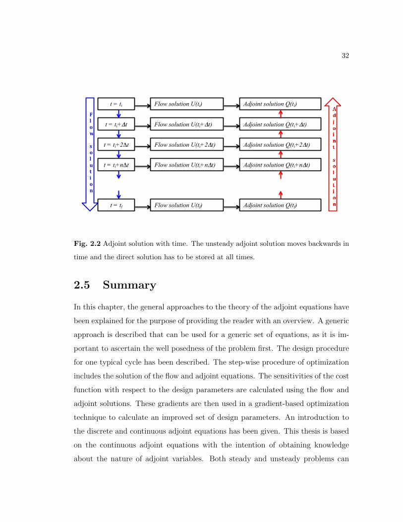
2.2. Adjoint solution with time. The unsteady adjoint solution moves back-wards in time and the direct solution has to be stored at all times. . . . 32
3.1. The centerline singularity for circular grid and a multi-block ‘H’ typegrid generation to avoid centerline singularity. . . . . . . . . . . . . . . . 43
4.1. The generation of multi-blocks showing grid singularities at the blockinterface. . . . . . . . . . . . . . . . . . . . . . . . . . . . . . . . . . . . 50
4.2. Multi-block ‘H’ type grid generation to avoid the centerline singularity. . 514.3. The mesh and multi-block topology for propagation of a Gaussian pulse
in a cube. . . . . . . . . . . . . . . . . . . . . . . . . . . . . . . . . . . . 554.4. Propagation of a Gaussian pulse through block interfaces at a) t = 0s,
b) t = 0.001s, c) t = 0.002s and d) t = 0.004s. . . . . . . . . . . . . . . 574.5. Comparison of analytic (solid) and numerical (symbol) solutions for Gaus-
sian pulse propagation. . . . . . . . . . . . . . . . . . . . . . . . . . . . . 584.6. The cross-section of the convergent-divergent nozzle with five blocks to
avoid centerline singularity. . . . . . . . . . . . . . . . . . . . . . . . . . 604.7. The comparison of direct and adjoint pressure contours. . . . . . . . . . 604.8. The comparison of direct and adjoint axial velocity contours. . . . . . . 614.9. The comparison of direct and adjoint cross-stream velocity contours. . . 614.10. The comparison of direct and adjoint density contours. . . . . . . . . . . 61
5.1. Nozzle contour, sensor and actuator regions. . . . . . . . . . . . . . . . . 655.2. The variation in pressure contours and streamlines, in the divergent sec-
tion of the nozzle, as the amplitude of the blowing velocity vb is variedto 0, 10, 30 and 60 m/s. . . . . . . . . . . . . . . . . . . . . . . . . . . . 74
5.3. Variation of the amplitude of the blowing vb in m/s with design cycles. 745.4. Decay of the cost function in Pa2 with design cycle. . . . . . . . . . . . 755.5. Removal of shock with adjoint design cycles. The sensor region is shown
as a box in the diverging section of the nozzle. . . . . . . . . . . . . . . 77
6.1. Variation of the blowing distribution with design cycles. . . . . . . . . . 996.2. Variation of the pressure distribution on the upper nozzle wall with design
cycles. . . . . . . . . . . . . . . . . . . . . . . . . . . . . . . . . . . . . . 1016.3. Two-dimensional nozzle domain and boundary conditions. . . . . . . . . 1026.4. The actuator and sensor regions on the divergent section of nozzle. . . . 1036.5. Pressure distibution for initial shocked flow. Area ratio = 1.12, NPR =
1.5, no blowing. . . . . . . . . . . . . . . . . . . . . . . . . . . . . . . . . 1056.6. Ideally expanded ‘desired’ pressure distribution. NPR = 1.5, area ratio
= 1.04, no blowing. . . . . . . . . . . . . . . . . . . . . . . . . . . . . . . 1056.7. Nozzle pressure distribution after two design cycles. NPR = 1.5, area
ratio = 1.12, with blowing. . . . . . . . . . . . . . . . . . . . . . . . . . 1066.8. Initial, first and desired pressure distributions on the nozzle centerline. . 1066.9. Nozzle showing surface mesh. . . . . . . . . . . . . . . . . . . . . . . . . 1086.10. Nozzle multi-block grid structure. . . . . . . . . . . . . . . . . . . . . . . 1096.11. The location of actuators (the blowing ports). . . . . . . . . . . . . . . . 109

x
6.12. The pressure distribution when there is no blowing in the divergent section. 1116.13. The pressure distribution with blowing in the divergent section. . . . . . 1116.14. Introduction of counter rotating stream-wise vortices due to blowing. . . 1126.15. Variation of the pressure difference on the nozzle wall between the current
and desired pressure distribution with design cycle. . . . . . . . . . . . . 1146.16. The decay of cost function with design cycles. . . . . . . . . . . . . . . . 1156.17. Pressure distribution on nozzle centerline with design cycles. . . . . . . 1166.18. Mach number distribution on nozzle centerline with design cycles. . . . 1166.19. Blowing velocity normal to the wall used to generate the desired pressure
distribution. . . . . . . . . . . . . . . . . . . . . . . . . . . . . . . . . . . 1176.20. Blowing velocity normal to the wall as given by fourth design cycle. . . 1176.21. The placement of blocks when the external domain is included. . . . . . 1196.22. The mesh including the external domain. . . . . . . . . . . . . . . . . . 1206.23. The location of symmetrically placed actuators in the nozzle diverging
section. . . . . . . . . . . . . . . . . . . . . . . . . . . . . . . . . . . . . 1206.24. The Mach number contours for the nozzle operating with 4.58 nozzle
pressure ratio and no blowing. . . . . . . . . . . . . . . . . . . . . . . . . 1216.25. The Mach number contours for the nozzle operating with 4.58 nozzle
pressure ratio and the desired blowing. . . . . . . . . . . . . . . . . . . . 1226.26. The Mach number contours after the first design cycle for the nozzle
operating with 4.58 nozzle pressure ratio. . . . . . . . . . . . . . . . . . 1226.27. The Mach number contours after the second design cycle for the nozzle
operating with 4.58 nozzle pressure ratio. . . . . . . . . . . . . . . . . . 1236.28. The Mach number contours after third design cycle for the nozzle oper-
ating with 4.58 nozzle pressure ratio. . . . . . . . . . . . . . . . . . . . . 123
A.1. The code structure to find direct and adjoint solutions and optimizationof the cost function - continued to next figure . . . . . . . . . . . . . . . 133
A.2. The code structure to find direct and adjoint solutions and optimizationof the cost function . . . . . . . . . . . . . . . . . . . . . . . . . . . . . . 134

xi
Nomenclature
Symbol Description
ρ density
p static pressure
T temperature
ξ, η, ζ orthogonal coordinate system in computa-tional domain
δij Kronecker delta
γ ratio of specific heats
λ spectral radius
σ CFL number
θ angle of injection
∆t numerical time step
c speed of sound
D nozzle exit diameter
et total energy per unit mass
F1, F2, F3 inviscid fluxes in the governing equations

xii
M Mach number
Md design Mach number
Mj jet Mach number
Po total or stagnantion pressure
To total or stagnantion temperature
pa ambient pressure
R gas constant of air at STP
u1, u2, u3 axial, vertical and spanwise velocity
(x, y, z) three directions in the physical space
Q vector of adjoint variables
vb blowing velocity
α design parameters
J cost function or objective function
L Lagrange functional
Subscript
0 total value
i, j, k indices in three computational directions
u derivative with respect to u
Superscript
′ the perturbation with respect to the flowvariables
Abbereviations
NPR nozzle pressure ratio

xiii
BBSAN broadband shock associated noise
OASPL overall sound pressure level
SPL sound pressure level
TTR total temperature ration
IPR injection pressure ratio
CD convergent-divergent

xiv
Acknowledgments
First and foremost, I would like to express my sincere gratitude to my advisor Prof.Philip Morris for his continuous support of my Ph.D. study and research. His im-mense patience and his vast knowledge are the reasons this thesis was possible.His continuous guidance has helped me in research and writing of this thesis. Hisqualities like hard work and punctuality have lasting impact on me as a researcher.
Besides my advisor, I would like to thank the rest of my thesis committee: Prof. D.K. McLaughlin, Prof. Mark D. Maughmer, and Prof. Dan Haworth for reviewingmy research work and providing with their valuable inputs.
I would especially like to thank the Penn State aeroacoustics experimental group,Dr. D. K. McLaughlin and Russell Powers for providing with the experimentaldata. My sincere thank goes to cluster admin Kirk Heller for his promptnessin troubleshooting the computer and cluster related problems. I would also liketo thank the Aerospace Department staff for their helpful attitude and friendliness.
I thank my labmates Yongle Du and Swati Saxena for their help in making meunderstand the concepts better and helping me with their deep knowledge of nu-merical implementation. I would also like to thank my fellow labmates VeeraManek and Monica Christiansen for making the lab a cheerful place.
Thanks to my special friends: Vishesh Karwa for endless discussions on how todo better research and Arnab Sengupta for his support and for lending me hiscomputer for finishing parts of my Ph.D., my awesome roommates RushmithaThiyagrajan and Rashmi Shukla for their dealing with my frustration and theirsupport in the most difficult times of my Ph.D. I would also like to thank Tanushree,Ragini, Himanshu, Kadappan, Nikhil, Ashish, Rakesh and Pankaj for making mystay at Penn State enjoyable. I would like to give a special mention of my lifelongfriends: Shraddha, Richa, Sangeeta and Vijaya for always believing in me and fortheir constant encouragement.

xv
My gratitude towards my husband Ashutosh Chauhan is inexpressible. This workwould not have been possible without him. His constant love and support comesin the most appropriate ways. He has helped me in all possible ways: encouragingme, pushing me, proof reading for me, cooking for me and just listening to mewhenever needed.
I would like to thank my best friend of all time, my sister Dr. Nimisha Singh whohas been an integral part of my life. Her guidance and support throughout my lifehas been invaluable to me. I dedicate this thesis to my parents: Mr. J. P. Sikarwarand Mrs. Sampada Sikarwar. My mother’s encouragement and belief are the solereasons for me being able to even imagine achieving anything in my life.

1
Chapter 1Introduction and Background
1.1 Motivation for Noise Reduction and Avail-
able Methods
The noise produced by the low bypass ratio turbofan engines used to power tactical
fighter aircraft is a problem for communities near military bases and for personnel
working in close proximity to the aircraft. For example, carrier deck personnel
are subject to noise exposure that can result in Noise-Induced Hearing Loss. This
results in disability payments that are made by the Veterans Administration each
year, costing over a billion dollars. Scientists have been struggling to achieve noise
reduction from tactical aircrafts for decades. The higher noise levels from tactical
aircraft put restrictions on the airbase operations and expansions. The number
of hours that Navy personnel can be exposed to such high levels is restricted.
According to military standards and regulations, a decrease in noise generation
by 3 dB can double the allowable exposure time. However, these restrictions are
not necessarily enforced. A recent study performed at Harvard School of Public
Health [7] shows that older people exposed to aircraft noise, especially at high
levels, may face increased risk of being hospitalized for cardiovascular disease. The
Federal Aviation Administration (FAA) pursues a program of aircraft noise con-
trol in cooperation with the aviation community. Noise control measures include
noise reduction at the source. That is, the development and adoption of quieter

2
aircraft, soundproofing and buyouts of buildings near airports, operational flight
control measures, and land use planning strategies. Similar noise reduction efforts
are being pursued by the Department of Defense.
Aircraft noise originates from three main sources: 1. Aerodynamic noise, 2. En-
gine and other mechanical noise and 3. Noise from aircraft systems. One of the
major contributors to the noise generated from the aircraft on take-off is the en-
gine exhaust noise. Other sources of sound from jet engines include fan noise,
combustion noise (low frequency and non-directional); and internal engine compo-
nent noise such as the turbine, struts and splitters (peaks at 60o from downstream
jet axis). The noise generated by an aircraft in the approach configuration has
two main contributions, the airframe noise resulting from turbulent flow over solid
structures like wings, slats, flaps and landing gears and the engine noise generated
from the jet and fan flows. The latter propagates in both the upstream and the
downstream directions. The dominant component of jet noise is due to the mixing
of large-scale turbulent eddies. The noise characteristics of supersonic jets are very
different from that of subsonic jets. Supersonic jets operating at off-design con-
ditions contain distinct components of turbulent mixing noise, broadband shock
associated noise and secreech. Figure 1.1 shows the different noise components in
an imperfectly expanded supersonic jet. On the other hand, subsonic jet noise is
mainly due to turbulent mixing and has a uniform broadband spectrum as shown
in figure 1.2.

3
Fig. 1.1 Far-field narrow-band noise spectra of a supersonic jet operating at Mj = 2.0
showing turbulent low frequency mixing noise, screeching tone and broadband shock
associated noise [40].
Fig. 1.2 Typical subsonic broadband jet noise spectra Sound Pressure Level vs. Strouhl
Number for a Mj = 0.9 jet [36].
Military aircraft engines are low bypass ratio turbofan engines that generate thrust
by exhausting a very high velocity jet. This jet is highly turbulent and hence there

4
are high levels of noise associated with the turbulent mixing of the jet plume with
the ambient air. Another noise component that exists is the broadband shock asso-
ciated noise (BBSAN) that occurs due to the fact that the engine does not always
operate at on-design conditions. When there is a difference between the ambi-
ent pressure and the nozzle exit pressure, there exist shock cells in the jet plume
through which the pressure adjusts to the ambient pressure. The interaction of
the turbulence in the jet shear layer with these shock cells (regions of alternating
pressure and temperature) results in the occurrence of BBSAN. In imperfectly ex-
panded supersonic jets, two additional components of noise arise: screech tones
and broadband shock associated noise.
Several methods have been proposed to reduce noise generated by high speed jets.
A recent summary of methods for high speed jet noise reduction is given by Morris
and McLaughlin [29]. The methods include microjet injection of air [1] or water [23]
downstream of the jet exit, chevrons [5, 13, 4], fluidic chevrons [21], plasma actua-
tors [39], beveled nozzles [47], conical and contoured nozzles with plasma actuators
[19] and corrugated nozzle inserts [42, 41]. The chevrons [5, 13] are used to reduce
noise from separate-flow turbofan engines. Mechanical chevron serrations at the
nozzle trailing edge generate axial vorticity that enhances jet plume mixing and
consequently reduces far-field noise. Fluidic chevrons as described by Kinzie et al.
[21] generated with air injected near the nozzle trailing edge create a vorticity field
similar to that of the mechanical chevrons and allow more flexibility in controlling
acoustic and thrust performance than a passive mechanical design. In addition, the
design of such a system has the future potential for actively controlling jet noise
by pulsing or otherwise optimally distributing the injected air. Plasma actuation
represents another active method to control aircraft noise as shown by Samimy
[39]. Some advantages of these methods are simplicity, the absence of mechanical
moving parts, and fast response. Experiments have shown that plasma actuators
can be used for flow control and airframe noise reduction. It is shown by Munday

5
et al. [32] that conical nozzles can exhibit reduction in far field noise generation.
Kim et al. [19] showed that contoured and conical nozzles with plasma actuators
can be helpful in noise reduction from Mach 1.65 jets. The reduction at shallow
polar angles is related to the decrease in the peak mixing noise level in both jets.
Experiments with microjets were performed with and without chevrons by Alk-
islar [1] and the effect of microject injection on vorticity generation and turbulent
characteristics was studied. It was observed that at an early location in the jet,
the influence of the microjet injection at the chevron tips is considerable. At the
injection locations within the shear layer, strong counter rotating vortex pairs were
created in addition to, but separate from, the ones created by the chevrons at the
chevron base. Their strength was comparable to those produced by the chevrons
alone; however, the pairs have an opposite sense of translation; their induced ve-
locities are opposite, with the chevron’s being away from the main jet and the
microjet’s being towards the main jet, at a location in the jet away from the noz-
zle exit both microjets and chevrons start to dissipate and lose their signature on
the flow.
The final method involves the insertion of corrugated seals into the diverging sec-
tion of a military-style convergent-divergent jet nozzle (to replace the existing
seals) as described by Seiner [42]. Figure 1.3 show the seals in a military style
nozzle divergent section. Seiner et al. [42] presented experimental and computa-
tional data for the noise changes with the use of two passive design modifications
that can be implemented with very little change in the nozzle geometry. They are
corrugated internal divergent secondary flap seals and external divergent primary
flap chevrons. Experimental measurements indicated that the noise was reduced
by 4dB relative to the baseline nozzle when corrugated seals were used and by 2
dB when chevrons were used. This technique has been shown to reduce both the
broadband shock-associated noise as well as the mixing noise in the peak noise ra-
diation direction. The corrugated seals work in two ways - they change the effective

6
area ratio of the nozzle and they introduce streamwise vortices in the jet plume.
The change in the effective area ratio helps to achieve nearly ideally expanded flow
even when the nozzle is working at an off-design condition at the time of take off
when the nozzle generally operates under-expanded. A reduction in broadband
shock associated noise is then observed. The introduction of streamwise vortices
helps to increase the turbulent mixing and thus reduces the mixing noise. The
original inserts were designed to be effective for take-off conditions where the jet
is over-expanded. The nozzle performance would be expected to degrade at other
conditions, such as in cruise at altitude.
Fig. 1.3 The corrugated seals for noise reduction as described by Seiner [41].
Recently, Morris et al.[30, 24] built on the corrugated seal concept, but instead
used fluidic inserts. This involves injection of air, at relatively low pressures and
total mass flow rates, into the diverging section of the nozzle. These fluidic inserts
deflect the flow in the same way as the mechanical inserts. But the fluidic inserts
represent an active control method, since the injectors can be modified or turned
off depending on the jet operating conditions. Details of the development of fluidic
inserts are given in the next section.

7
1.2 Fluidic Inserts
Fluidic inserts are noise reduction devices proposed at Penn State by Morris et
al.[30]. The idea is to achieve similar effects as the corrugated seals by using
carefully distributed blowing on the divergent section of the nozzle wall. The
bypass air would be used at relatively low pressure and low mass flow rates. It
is expected that there will not be much difference in the engine performance due
to the low mass flow rate. The experimental set-up and CAD design of fluidic
inserts is shown in figures 1.4 and figurecad respectively. The experiments have
been conducted at Penn State by McLaughlin et al.. An efficient methodology for
the simulation of heated jet is made possible since helium-air mixtures are used to
simulate the heated jets [8, 27]. Noise reductions in the peak noise direction of 4
to 5 dB have been achieved at model scale and broadband shock-associated noise
is effectively suppressed. The reduction in noise is dependent on the ratio of mass
flow rates for the injection and the core jet flow. Experiments on fluidic inserts
with simulated forward flight were performed at Penn State by Powers et al. [38].
Fluidic inserts in the presence of forward flight streams have shown a peak mixing
noise reduction of 4 dB and broadband shock associated noise reduction of 3 dB.
Comparisons of the acoustic spectra of the fluidic inserts nozzle and corrugated
seals nozzle have been made. Figure 1.6 shows the typical acoustic spectrum for
the baseline nozzle, the nozzle with three corrugated seals placed symmetrically
and the nozzle with three fluidic inserts places symmetrically on the nozzle wall.
The design Mach number of the nozzle is 1.56 and mass flow rate of the fluidic
inserts with respect to the core mass flow rate is 3.8%. The acoustic reductions
generated by the fluidic inserts are same as that of the corrugated seals. The
reduction in OASPL is of the order of 3 - 4 dB. The screech tones are removed
completely for both fluidic inserts and corrugated seal nozzles.

8
Fig. 1.4 The experimental set up for fluidic inserts. There are three inserts placed
symmetrically in the divergent section of the nozzle. There are two injectors per fluidic
insert.
Fig. 1.5 The CAD design of fluidic inserts.

9
(a) Corrugated seals (b) Fluidic inserts
Fig. 1.6 The acoustic spectrum of the baseline nozzle, a) corrugated seals and b)
fluidic inserts , Mj = 1.36, NPR = 3.0, TTR = 3.0 and injection mass flow ratio =
3.8%.
There are many advantages to the fluidic insert noise reduction technique. The
rate of blowing can be changed during flight. Thus, it would be very flexible.
Various blowing rates and distribution could help in making the engine operate
at near on-design conditions for all flight regimes. This would not only reduce
the noise but would also help in improving the performance. It is planned to use
the bypass air as the blowing fluid. Hence the implementation of the technique
would be convenient. Few new mechanical changes in the existing nozzle would be

10
required, apart from the installation of the flow control.
A schematic of how the fluidic inserts affect the flow is shown in figure 1.7. The
incoming flow due to the blowing on the nozzle wall shifts the streamlines away
from the nozzle wall, thus changing the effective exit to throat area ratio, as shown
in figure 1.7. The change in exit to throat area ratio changes the effective operating
conditions for the nozzle. Figure 1.8 shows the shifting of the flow by the shift
in streamlines caused by the two actuators. Early numerical experiments were
performed by Morris et al. [31] to see the effects of the inserts on the jet flow.
The modification in the jet plume due to the placement of the fluidic inserts is
shown in a numerical shadowgraph in figure 1.9 [34]. The nozzle pressure ratio
NPR is 4.58 and the design Mach number is 1.65. Figure 1.9a shows the baseline
unheated jet. Figure 1.9b shows a shadowgraph with one fluidic insert on the nozzle
wall. The shock cell structure is tilted from the centerline in the case with one
fluidic insert. Figure 1.9c shows the shadowgraph with two fluidic inserts placed
symmetrically. The shock cell structure for the two fluidic inserts is narrowed
towards the centerline. The placement of fluidic inserts in both cases change the
shock cell structure in the nozzle jet flow significantly. An optimized location of
the fluidic inserts with an optimum mass flow rate (or injection pressure ratio)
can be incorporated to achieve shock free flow field even when the nozzle is over-
expanded. This technique can be used to achieve a reduction in the broad band
shock associated noise from the nozzles operating at off-design conditions.

11
Fig. 1.7 The schematic of fluidic inserts. Flow streamlines shift away from the wall to
produce a new effective area ratio.
Fig. 1.8 The shifting of the streamlines in the nozzle with distributed blowing.

12
(a) The baseline nozzle [31]
(b) With one fluidic insert [31]
(c) With two fluidic inserts [31]
Fig. 1.9 Numerical shadowgraph with different fluidic inserts. Unheated, design Mach
number 1.65 and nozzle pressure ratio NPR = 4.58. The injection pressure ratio = 4.58.

13
The fluidic inserts are also known to introduce streamswise vortices into the jet
plume. Figure 1.10 shows the generation of counter-rotating vortices. There are
two actuators (or fluidic inserts) placed symmetrically shown by the black lines
and the vorticity generation from these actuators is shown by the counter-rotating
vortices. The generation of those counter rotating vortices is seen by the positive
and negative streamwise vorticity on the two sides of each actuator. The generation
of counter rotating vortices produce the effects similar to the corrugated seals.
The turbulent mixing in the jet shear layer is enhanced due to the introduction of
streamwise vortices and a reduction in mixing noise is achieved due to the increased
turbulent mixing in the jet shear layer.
Fig. 1.10 The generation of counter rotating streamwise vortices at each actuator.
An optimum placement of the fluidic inserts with optimum mass flow rates could
result in a greater reduction in the broadband shock associated and turbulent mix-
ing noise. Optimization of the placement and rate of injection is a challenge to

14
obtain the best effects from the fluidic inserts. There are multiple parameters to
be considered in the design of the fluidic inserts. These include the number and
location of the injectors and the pressures and mass flow rates to be used. The
optimization of these parameters is the next goal in the development of fluidic
inserts. These could be optimized on an ad hoc basis with multiple experiments
or numerical simulations. Alternatively an inverse design method could be used.
The adjoint approach is an inverse design optimization method that can be used
to optimize a problem with many design parameters. The objective of this the-
sis is to develop an adjoint method to find that rate of blowing in the nozzle to
achieve desired effects. The desired effects are quantified by the pressure distri-
bution associated with the nozzle. It is shown that an adjoint design approach
can be used to achieve a desired pressure distribution. The primary advantage
of using an adjoint method is that computational cost associated with the adjoint
approach is considerably less than that of the traditional inverse design approaches.
The next section provides some background on adjoint design methods. The origi-
nal use of adjoint methods in the area of aerodynamic design have been associated
with shape modification. A study of the use of adjoint methods for shape opti-
mization is followed by a description of the adjoint approach to incorporate active
flow control optimization [44, 45].
1.3 Use of Adjoint Method
Adjoint equations have been used for some time in optimal control theory. Li-
ons [26] used adjoint methods to develop an optimization technique for systems
that are governed by partial differential equations. Pironneau [37] used the adjoint
method for the first time in fluid dynamics for design work, but Jameson [14, 15]
revolutionized the use of adjoint methods for aerodynamic design. He developed
continuous adjoint methods for different governing equations including the poten-
tial, the Euler, and the Navier-Stokes equations. An optimal design is one that

15
optimizes the defined cost function within given constraints. Jameson showed that
the adjoint method can be used to modify the shape under consideration such as
airfoil, wing or full aircraft to achieve a reduction in the cost function. The cost
function could be either the lift or drag coefficients or some difference relative to
a desired flow behavior. Joslin et al.[16] developed an automated methodology for
active flow control using adjoint methods. A method for the suppression of two-
dimensional instability waves for a flat plate boundary layer was incorporated, by
implementation of blowing and suction at the wall. The problem was treated as
a control problem with the rate of blowing (or suction) acting as the control. It
was found that no prior knowledge of the instability characteristics was required
to optimize the control (blowing). Noise control based on adjoint methods has
also been explored by Wei and Freund [49]. Freund [10] attempted to understand
the workings of the jet noise mechanism with the use of adjoint methods. These
studies were based on the aerodynamic optimization approach by Jameson and
turbulence control by Bewley [2]. Wei and Freund minimized the noise radiated
by a two-dimensional mixing layer for a line of observers above the layer. The
time dependent Navier-Stokes equations and the associated adjoint equations were
solved to determine the time history of various controllers near the origin of the
mixing layer. Wei and Freund showed that a two dimensional mixing layer can be
made quieter based on the concept that the flow also works as a source of sound.
The actuation was taken as a general inhomogeneity in the flow equations with
support near the inflow boundary. It did not correspond to any particular actuator.
The near-nozzle jet was modeled by a randomly excited two-dimensional mixing
layer. Mixing layers between streams with Mach numbers 0.2 and 0.9, which is
a subsonic case, were studied. The controls were implemented as general source
terms. That is, body forces, mass sources and internal energy sources. The internal
energy control was found to be the most effective with a reduction of 11 dB in the
noise intensity. It was shown that the noise reduction was not achieved by noise
cancellation, but from a genuine change in the flow as a noise source. The changes

16
observed in the flow gross features were very subtle. However, the decomposition
of the flow into empirical eigenfunctions showed that the downstream advection of
turbulent structures takes place more uniformly with the excitation. Kim et al.[18]
extended these ideas to a Mach 1.3 jet with some success. Kim tried to reduce
the turbulent jet noise by implementing various flow controls that would change
the flow turbulence. The benefit of this approach is that the ‘actuator region’ can
exist anywhere in the domain. They found the gradient of the cost function with
respect to the control using adjoint methods. This gradient was then used to find
the local optimum of the cost function with respect to the control. The conjugate
gradient method was used to minimize the cost function. Far field noise, beyond
the computational domain, was predicted using a solution to the Ffowcs Williams
and Hawkings equation [3]. The total number of optimization parameters was 280
x 106. A reduction of 2.6% was observed in the value of cost function over the
entire domain.
1.4 The Adjoint Approach
The adjoint optimization method is a constrained optimization technique. The
adjoint approach works as a ‘feedback - control’ approach where the feedback from
the sensor is communicated back to the control. Then the control is modified based
on the feedback and generates a new flow. The same process is repeated until the
change in the flow is small. Figure 1.11 illustrates this cycle. The adjoint equations
are developed in such a way that the flow governing equations are considered as
the constraints for the optimization of a given cost function. The resultant adjoint
equations produce the gradients of the cost function with respect to the design
parameters without having to calculate the change in flow variables with respect
to the design parameters. This saves considerable computational cost. The adjoint
method works as a control technique in which a sensor provides a measure of the
cost function. The adjoint equations are then solved for the sensitivity of the

17
respective cost function to the control. This information is then passed to an
actuator or controller, so that the flow is driven towards the desired state.
Fig. 1.11 The adjoint design approach.
1.5 Passive Control Using Adjoint Method
The use of an adjoint design method for nozzle shape design is illustrated in this
section, the details of this analysis are given in Sikarwar [43]. Adjoint methods were
implemented to find the optimum change in the geometry such that a defined cost
function was minimized. The formulation was based on Jameson’s [15] approach.
The geometry was dependent on a set of design parameters and the cost function
was defined as the difference between a desired and calculated nozzle centerline
pressure. The adjoint approach was validated by calculating the desired pressure
difference using a known set of design parameters. That is, for a known geometry
the centerline pressure was calculated and was considered as the desired pressure
distribution. Then the geometry was perturbed from this desired geometry by
changing the design parameters. Then the adjoint method was used to recover the

18
desired pressure distribution. Figure 1.12 shows the distribution of pressure on the
nozzle centerline. The initial pressure distribution is shown by a red line. The final
pressure distribution is shown by a blue line. The desired pressure distribution is
shown by the symbols. All these calculations are performed for a fixed value of
nozzle pressure ratio NPR = 1.5. Initially, the shock is at the nozzle exit and keeps
moving inside the nozzle with each design cycle. The final and desired pressure
distributions do not agree exactly but they are very close. The initial value of the
cost function is 4.39 x 10⁶ Pa which drops to a value of 2.13 x 10⁵ Pa after 32 design
cycles for a decrease of 95.14% in the cost function. The full flow solutions given
by pressure contours, for the initial (upper) and final (lower) geometries inside the
nozzle domain, are shown in Figure 1.13. The difference in the two solutions is the
shock location. The nozzle is sonic at the throat, hence, the flow upstream of the
throat remains the same; whereas, the flow downstream changes with each design
cycle.

19
Fig. 1.12 The distribution of pressure (with respect to total pressure Po) along the
nozzle centerline. The red and blue lines show the initial and final pressure respectively.
The desired pressure is shown by black symbols.
Fig. 1.13 Pressure contours inside the nozzle domain. The upper half shows the initial
flow and lower half shows the final flow.

20
The nozzle geometries are shown in figure 1.14. The red line shows the initial
geometry. The black line shows the desired geometry and the green line shows the
final geometry given by the adjoint design method.
Fig. 1.14 The geometry of the nozzle. Calculations were performed for only half the
domain. The red line shows the initial geometry. The green line shows the final geometry.
The black line shows the geometry that gives the desired pressure distribution.
1.6 Thesis outline
The objective of this thesis is to develop an adjoint approach for the optimization
of blowing in the diverging section of a convergent-divergent (CD) nozzle. The
adjoint approach developed in this thesis considers the blowing velocities as the
control parameters that are optimized. The next chapter describes the general
theory and development of adjoint optimization. The details of the discrete and
continuous adjoint approaches and steady and unsteady problems are given in this
chapter. The adjoint optimization procedure for a typical design cycle is described.
Chapter 3 describes the numerical methods implemented in the development of the
solver. The details of the numerical schemes, artificial dissipation and convergence
acceleration techniques are given in this chapter. The solver developed for the

21
proposed research is a multi-block structured solver. The multi-block mesh topol-
ogy includes block interfaces where there may be grid singularities between two
adjacent blocks. These grid singularities introduce numerical errors into the solu-
tion. A characteristics-based block interface boundary condition is implemented
to overcome this issue for both direct and adjoint equations. The details of the
boundary conditions as well as discussion on the nature of the adjoint variables are
given in Chapter 4. Two different adjoint approaches have been developed in the
course of this study. The difference in the two approaches is in the consideration
of the control. Chapter 5 describes the first approach where the blowing velocity
is given by a combination of basis functions multiplied by weighting coefficients.
These coefficients are considered as the design parameters for the optimization.
The second approach where the blowing velocities are considered as free controls,
is described in Chapter 6. The velocity components at each grid point in the actu-
ator region serve as the control parameters for the adjoint approach. The details
of the solver developed for this research are given in Appendix A. The conclusions
and ideas for future work are given in chapter 7.
1.7 Original Contribution of the Thesis
The traditional uses of adjoint methods have been in the area of shape optimiza-
tion. There has been little work on the use of adjoint methods for active flow
control. Though some examples exist in the literature where an adjoint optimiza-
tion technique has been used for the optimization of blowing, those problems are
restricted to two-dimensional incompressible calculations for simple geometries.
Adjoint methods have not been used to optimize control in nozzle flows. The work
presented in this thesis is novel in the sense of the application and also in the sense
of the development of the method. A new adjoint method to optimize distributed
blowing on the nozzle wall to achieve a desired pressure distribution in the nozzle
has been developed. Two different adjoint approaches have been developed and

22
implemented.
An adjoint approach, where distributed blowing in a nozzle is considered as control,
has been developed. The blowing velocity at each grid point of an actuator region
has been considered as an independent control parameter. New adjoint boundary
conditions based on the direct flow boundary conditions have been developed. For
the numerical implementation of the new approach for complex geometries, two-
and three-dimensional direct and adjoint solvers have been developed. A solver to
calculate the sensitivities of the cost function with respect to the control parame-
ters using the direct and adjoint solutions has been developed for the optimization.
These sensitivities are used to determine the blowing distribution that minimizes
the cost function.
To perform three-dimensional calculations for more complicated geometries a multi-
block grid topology has been used. A new technique to treat the block interfaces
while performing the adjoint calculations has been developed. This characteristics-
based block interface boundary condition for the adjoint equations has been de-
veloped and implemented for the first time. The numerical implementation of the
direct and adjoint block interface boundary conditions has been incorporated into
the direct and adjoint solvers. The direct and adjoint solvers are equipped to work
with multi-block structured grids with arbitrary orientations. The communication
of data at arbitrarily indexed block boundaries has been incorporated.
The next chapter provides a general development of the adjoint optimization
method.

23
Chapter 2General Development of the AdjointMethod
The scope for the uses of the adjoint method is very wide. As the general interest
in the use of the adjoint method is increasing, a variety of problems are being
solved using this approach. Some of the many areas where the adjoint method has
been used for the optimization include statistics [22], weather predictions [17], ge-
ometry optimization [11, 15], mesh improvements [35] and error analysis [46]. The
use of the adjoint approach varies by disciplines, goals etc. However, the general
approach remains the same. In this chapter the basic theory of the adjoint method
is described. Since there are two ways to develop the adjoint equations - discrete
and continuous - an introduction to both these approaches is given in this chapter.
This chapter provides the basis for the research work presented in this thesis. The
particular approaches used in this thesis can be better understood once the basic
approach is clear. The approach can be modified to solve specific problems using
the flow model and cost function specific to the problem. If the desired pressure
distribution inside a nozzle is known, an adjoint method can be used to find the
design parameters corresponding to the desired pressure distribution. For the su-
personic case, when there are shocks in the nozzle, this method can be used to
find a set of design parameters such that the shock strength is minimized, and by
inference, so would be the broadband shock associated noise. The various goals
can be facilitated by changing the cost function, which is a measure of the desired

24
behavior. Various design problems can be addressed by changing the control pa-
rameters or design parameters, but the basic approach for a general cost function
and general design parameters remains the same and this is described in the next
section.
2.1 General Approach
The basic theory of the adjoint method explained in this section is based on Jame-
son’s [14] approach. It is a constrained optimization method where the governing
equations are considered as constraints. The theory presented in this section is
generic to the development of the adjoint method and can be implemented for any
set of governing equations, for any design parameters, and for any choice of cost
function (within the mathematical admissible limits). The optimization technique
is based on the gradient descent method. However, it is computationally expen-
sive to calculate the gradients directly. Adjoint methods can be used to calculate
these gradients using a significantly reduced computational cost. The adjoint equa-
tions are developed such that the changes in the flow variables with respect to the
control/design parameter are not required to be calculated while determining the
sensitivity of the cost function to the design parameters. The elimination of the
need to calculate the change in the flow variables with respect to the change in
design parameters reduces the computational cost required to calculate the gradi-
ents with respect to the design parameters significantly.
The starting point is a system of nonlinear partial differential equations governing
the flow in the computational domain. Design parameters are denoted by α. The
flow equations and the cost function are dependent on the flow solution vector U
and the design variables α.
The governing equations are given by,
R = R(U, α) = 0. (2.1)

25
The cost function is a measure of the desired behavior. The adjoint method is
used to minimize or maximize the cost function. It could be a measure of lift or
drag over an airfoil or it could be a measure of pressure drop in a pipe. There are
several choices for the cost function based on the statement of the problem. The
cost function is also a function of the flow variables U and design parameters α.
In general, the cost function J is given by,
J = J(U, α) (2.2)
Any change in the design parameters would cause a change in the flow variables
as well, which would cause a change in the cost function. The changes in the cost
function and the governing equations with respect to the flow and design variables
are given by,
δJ =∂JT
∂αδα +
∂JT
∂UδU (2.3)
and,
δR =∂R
∂αδα +
∂R
∂UδU = 0 (2.4)
The augmented change in the cost function is the change in cost function when
the change in the governing equations is considered a constraint. The augmented
change in cost function when relation (2.4) is used is given by,
δJ =∂JT
∂αδα +
∂JT
∂UδU −QT
(∂R
∂αδα +
∂R
∂UδU
)(2.5)
Here, Q is the vector of adjoint variables and acts as a Lagrange multiplier. It
should be noted that augmentation of the cost function does not change the value
of the cost function since the governing equations are always satisfied and are equal
to zero. Expression (2.5) can be rearranged such that the terms dependent on the
change in the flow variables δU are brought together as are the terms dependent
on the change in the design parameter δα.

26
δJ =
(∂JT
∂α−QT ∂R
∂α
)δα +
(∂JT
∂U−QT ∂R
∂U
)δU (2.6)
The goal is to eliminate the requirement to calculate the change in flow variables
δU . This is achieved by choosing the adjoint variables to satisfy the equation,
∂JT
∂U−QT ∂R
∂U= 0 (2.7)
This equation is known as the “adjoint equation”, and can be solved to calculate
the value of the vector Q. The boundary conditions for the adjoint equations are
derived based on the boundary conditions for the direct flow equations.
The sensitivity of the objective function δJ is independent of the flow solution
perturbation δU and is given by,
δJ =
(∂JT
∂α−QT ∂R
∂α
)δα (2.8)
or, the sensitivity of cost function with respect to the design parameters is given
by,δJ
δα=
(∂JT
∂α−QT ∂R
∂α
)(2.9)
Once the values of the adjoint variables are known, equation (2.9) is used to cal-
culate the sensitivities of the cost function with respect to the design parameters.
These sensitivities are used in any gradient optimization method to find the opti-
mum values of the design parameters α.
This section has explained the general formulation of the adjoint method. The
approaches for the particular cases of interest in this thesis are explained in more
detail in chapters 5 and 6.

27
2.2 Outline of the Design Procedure
An outline of the optimization procedure is summarized in figure 2.1. More steps
can be added to the process based on requirements such as when there is shock
in the solution. In this case an extra step can be added for smoothing the cost
function. When geometry optimization is considered, an extra step to generate
a new mesh is added, because a new mesh has to be generated for a new set of
design parameters. In the present research the geometry has been kept fixed and
it is not required to generate a new mesh for a new set of design parameters. The
basic steps of the design process are,
1. Fix the initial set of design parameters:
First the initial values of the design parameter are chosen. In theory, this
choice is arbitrary but the convergence of the adjoint design cycle is dependent
on it so a wise guess is advisable. In the case when the blowing velocity is
considered as the design parameter, the cycle is started either with a zero
initial blowing velocity or a very small value.
2. Solve the flow equations for this set of design parameters:
The flow equations are then solved for the design parameters fixed in the
previous step. The flow equations are solved by marching in time to a steady
state and an appropriate initial condition for the flow variables is required.
3. Solve the adjoint equations:
Once the flow solution is obtained, the adjoint equations are solved for the
fixed set of design parameters. The adjoint equations are also solved by
marching in time to a steady state, and again it is important to chose an
appropriate initial condition for the adjoint variables.
4. Calculate the gradients:
The gradients are dependent on both the adjoint and flow solutions and can
be calculated using direct algebraic relations.

28
5. Find the new set of design parameters using the gradients:
The gradients calculated in the previous step are used in a gradient based
optimization technique such as steepest decent or conjugate gradient methods
to calculate the next set of design parameters.
6. Repeat the cycle until convergence:
The cycle is repeated until the cost function reduces to a required minimum.

29
Solve flow equations
STOP
Solve adjoint equations
New design parameters
Calculate gradients
Calculate Cost Function
If C.F. < Tolerance
Fig. 2.1 The main steps of the optimization procedure.
2.3 Discrete and Continuous Approaches
The adjoint equations are dependent on the direct flow equations. As the form of
direct flow equations considered varies, the development of the adjoint variables
also varies. There are two main approaches in which the adjoint equations can

30
be developed. These are the discrete and continuous approaches. The discrete
approach is such that the discretized direct flow equations are considered first
and then the set of adjoint equations is developed. The adjoint equations derived
in this manner are already discretized and no further discretization is required.
The continuous approach is the one where the continuous direct flow equations
are considered. The continuous adjoint equations are then discretized using the
discretization scheme of choice. In most cases the continuous adjoint equations
are discretized using the same numerical scheme as the direct equations. The
differences in the two approaches can be summed up as calculating the exact
gradient of the inexact cost function (discrete adjoint) or the inexact gradient of
the exact cost function (continuous) [33].
In the appropriate limits, when space and time intervals go towards zero, the
discrete adjoint equations converge to the continuous adjoint equations and the
discrete adjoint boundary conditions converge to the continuous adjoint boundary
conditions.
lim∆x,∆t→0
Discrete Adjoint Equations⇒ Continuous Adjoint Equations
lim∆x,∆t→0
Discrete Adjoint BC⇒ Continuous Adjoint BC(2.10)
There are pros and cons to both approaches. The continuous approach provides
an insight into the behavior and nature of the equations but it may be difficult to
obtain a stable solution. The boundary conditions for the continuous approach are
derived separately. The discrete approach is relatively easy to implement especially
because no direct derivation of the boundary conditions is required for the discrete
adjoint variables, but it is difficult to infer the meaning of the adjoint variables.
The present work is based on the continuous approach, since it is intended to
obtain an insight into the form of the adjoint equations and the behavior of adjoint
variables. A characteristic analysis of the adjoint equations was possible because
of the choice of the continuous approach. The nature of the adjoint characteristics

31
and the development of boundary conditions based on the adjoint characteristics
are given in chapter 4.
2.4 Steady and Time Dependent Problems
The adjoint approach can be used for both, steady and unsteady problems. As
expected, the adjoint variables corresponding to the unsteady flow variables are
unsteady in nature. The time dependent adjoint solution can be obtained as shown
in figure 2.2. The adjoint equations are solved backwards in time, the details of
the mathematical development of the unsteady equations are given in chapter 6.
Adjoint variables are dependent on the direct flow variables, when the adjoint
solution is marched backwards in time from the final time of calculation, t = tf , to
the initial time of calculation, t = ti, the direct flow solution has also to march from
the initial time, t = ti to final time, t = tf . Therefore, before starting the adjoint
calculation, it is required to have the direct flow solution available at all times. This
condition increases the memory requirement tremendously, especially for problems
where the grid sizes are large. Researchers have tried several manipulations to
handle the storage of solutions better. These include storing the solution at few
time intervals and solving for the remainder [48, 25]. But, none of the known
manipulations are very effective. Keeping the memory requirements in mind, only
the steady state solutions of adjoint and direct equations are obtained in this thesis.
Even though artificial time marching is incorporated to march to the steady state,
only the steady state solution for the direct flow equations is stored and is kept
fixed when marching to the steady state of the adjoint equations.
32
t = ti
t = ti+Δt
t = ti+2Δt
Flow solution U(ti)
Flow solution U(ti+Δt) Adjoint solution Q(ti+Δt)
Adjoint solution Q(ti)
Flow solution
t = ti+nΔt
t = tf
Flow solution U(ti+2Δt)
Flow solution U(ti+nΔt)
Flow solution U(tf)
Adjoint solution Q(ti+2Δt)
Adjoint solution Q(ti+nΔt)
Adjoint solution Q(tf)
Fig. 2.2 Adjoint solution with time. The unsteady adjoint solution moves backwards in
time and the direct solution has to be stored at all times.
2.5 Summary
In this chapter, the general approaches to the theory of the adjoint equations have
been explained for the purpose of providing the reader with an overview. A generic
approach is described that can be used for a generic set of equations, as it is im-
portant to ascertain the well posedness of the problem first. The design procedure
for one typical cycle has been described. The step-wise procedure of optimization
includes the solution of the flow and adjoint equations. The sensitivities of the cost
function with respect to the design parameters are calculated using the flow and
adjoint solutions. These gradients are then used in a gradient-based optimization
technique to calculate an improved set of design parameters. An introduction to
the discrete and continuous adjoint equations has been given. This thesis is based
on the continuous adjoint equations with the intention of obtaining knowledge
about the nature of adjoint variables. Both steady and unsteady problems can
33
be solved using the adjoint approach. However, the unsteady adjoint equations
have vast memory requirements to store the flow solution at all times. This is the
primary reason why steady problems are solved in the present thesis.
The development of the adjoint equations for specific problems and their solutions
are given in chapters 5 and 6. The next chapter describes the numerical method
used to find the solution of the adjoint and direct problems. Details of time
marching and discretization techniques are given. Several schemes are used to
accelerate the convergence and to stabilize the solution. A detailed description of
these schemes is also given. The grid indexing is arbitrary at the block interfaces
mentioned above and there can be numerical issues if differences are not accounted
for. A technique to generalize the grid indexing for each block is discussed in the
next chapter.

34
Chapter 3Numerical Method
The goal of the research described in this thesis is to use an adjoint optimization
method for the optimization of the blowing velocity in the divergent section of
a nozzle to achieve a modification of the flow with the ultimate goal of reducing
noise. The nature of the adjoint and flow equations is very similar as discussed in
more details in chapter 4. This property is the basis of making the assumption
that both adjoint and direct flow equations can be solved on the same mesh. The
direction of propagation of the adjoint characteristics are opposite to the direction
of propagation of the direct flow equations and the adjoint equations are solved
backwards in time. The time step is negative for the time integration of the adjoint
equations but the numerical scheme for time integration is same as for the direct
flow equations. This chapter describes in detail the numerical techniques that have
been implemented for the solution of the direct and adjoint problems.
A direct flow solver and a corresponding adjoint solver have been developed for
implementing the adjoint optimization. The solver works on multi-block structured
grids. An example of the grid topology is shown in figure 4.2. The block interfaces
of multi-block meshes have grid singularities that can introduce numerical errors
in the solution. Such block interfaces are treated with the use of characteristics-
based boundary conditions. These conditions have been developed for the direct
as well as the adjoint flow equations. The adjoint flow equations behave differently

35
from the direct flow equations so the treatment is different for the adjoint block
interfaces. These boundary conditions are discussed in detail in chapter 4. The
main numerical attributes of the solver include the implementation of local time
stepping for better convergence rate and the use of implicit residual smoothing
for additional faster convergence. Various numerical schemes have been used for
the discretization of the spatial derivatives and for time marching. These schemes
include a MacCormack scheme, second and sixth order central differencing and
traditional and modified Runge-Kutta time marching algorithms. The details of
these schemes are given in the next section.
3.1 Numerical Schemes
This section describes the spatial discretization and time marching schemes. There
are several options for spatial discretization. These options include MacCormack
and central differencing schemes. These schemes are described in the following
sections.
3.1.1 MacCormack Scheme
It has been mentioned that one of the goals of this thesis is to provide a method for
generating shock-free flows for the purpose of reducing broadband shock associated
noise. This has been a key point to consider while choosing the numerical scheme.
The MacCormack scheme is very good for capturing shocks in a solution. The
governing flow equations are solved in conservative form for the same reason. A
second order MacCormack scheme includes two steps: the predictor step where
the solution is predicted using a forward difference in space at a half time step and
the corrector step, where the solution is corrected using the predicted half step
solution and a backward difference scheme. These steps are described below.
The governing flow equations in conservative form are given by,
∂U
∂t+∂Fi∂xi
= 0 (3.1)
36
The following two steps explain how the MacCormack scheme is used to discretize
the above set of equations.
Predictor step:
Predicted values of the time derivatives are calculated in this step and this value
is then used to correct the values in the next step.
∂U
∂t
∗= −
(∂Fi∂xi
)FD
(3.2)
Where, (∂Fi∂xi
)FD are the spatial derivatives calculated using a forward differencing
scheme. The discretization is illustrated at the point ‘j′ with grid spacing ‘h′ as,
(∂Fi∂xi
)FD
=F j+1i− F j
i
h(3.3)
Corrector step:
The time derivatives calculated above are used to correct the values of the time
derivative as follows,∂U
∂t
∗∗= −
(∂F ∗
i
∂xi
)BD
(3.4)
Where, (∂F ∗
i
∂xi)BD are the spatial derivatives calculated using a backward differencing
scheme. The discretization is illustrated at the point ‘j′ with grid spacing ‘h′ as,
(∂F ∗
i
∂xi
)BD
=F ∗ji− F ∗j−1
i
h(3.5)
Note that the predicted values of fluxes F ∗i
have been used here to calculate the
corrected time derivatives.
These two time derivatives are now used to calculate the average time derivative,
given by,∂U
∂t=
1
2
(∂U∗
∂t+∂U∗∗
∂t
)(3.6)
This value of time derivative is used to calculate the values of the solution variables
at the next time step. The MacCormack scheme is second order in time and space

37
and is very good at capturing discontinuities in the flow. The above discretiza-
tion is illustrated here for the direct equations of motion. The same process is
implemented for the discretization of the adjoint equations. The adjoint equations
can not be written in conservative form and are used as given for discretization
purposes.
3.1.2 Central Difference Schemes
There are several central difference schemes that have been developed by re-
searchers for various numerical requirements. A central difference scheme can
be used with an appropriate time marching scheme for marching iteratively to the
steady state. There are a few advantages of using these schemes over using the
MacCormack scheme. The most important advantage is that local time stepping
can be used for a faster convergence to steady state solution. It was observed
that when combined with MacCormack scheme, local time stepping does not al-
ways converge to the correct solution. To increase the rate of convergence while
maintaining the order of accuracy of the solution, several more schemes have been
implemented. There are options available for using either a second or sixth or-
der central difference scheme based on the specific requirement of the simulation.
When acoustic predictions are not being performed, a second order scheme can be
used. The stencil for this scheme is given by,
∂Fii∂xi
=1
2
Fii+1− Fii−1
h, (3.7)
where h is the uniform grid spacing between i− 1, i and i+ 1 grid points.
3.1.3 Time Marching Schemes
Even though the equations and solutions considered for this work are steady, artifi-
cial time marching has been implemented to march the solution to a steady state.
A number of time marching schemes have been implemented and a comparison
between them has been carried out as described in the following section. First, an

38
introduction of these schemes is given followed by a comparison of the convergence
rates for the various time marching schemes. Finally, local time stepping is used
to increase the rate of convergence to a steady state. An introduction to local time
stepping is provided in the final part of this section.
Traditional Runge-Kutta Time Marching
Runge-Kutta methods are a family of implicit and explicit time marching schemes
that were developed in 1900’s by the German mathematicians C. Runge and M.
W. Kutta. These time marching schemes were developed for finding approximate
numerical solutions of ordinary differential equations. These methods are high
order non linear methods that can be used for marching the solution from one
time step to the next. A generalization of the method is possible for k stage time
marching where there are k stages between two time steps n and n+ 1. Consider
an equation of the type,
U ′ = H (3.8)
where,
H = H(U, t) (3.9)
and U ′ is the derivative of U with respect to time t. To find the solution at the n+1
time step, when the solution at the n time step is know, the following algorithm

39
is followed,
U (1) = Un (3.10)
U (2) = Un + ∆tα2H(1) (3.11)
U (3) = Un + ∆tα3H(2) (3.12)
. (3.13)
. (3.14)
U (k) = Un + ∆tαkH(k−1) (3.15)
U (n+1) = Un + ∆tk∑k=1
βkH(k) (3.16)
Here, H(k) depicts the time derivative at the stage k, and is calculated using the
right hand side of the differential equation calculated using the solution at that
stage: H(k) = H(U (k)). The coefficients βk must satisfy the consistency equation,
k∑i=1
βi = 1 (3.17)
A traditional Runge-Kutta method is the 4 stage classical Runge-Kutta method,
often referred to as the RK4 method. The coefficients for this method are given
by,
α2 =1
2, α3 =
1
2, α4 = 1
β1 = β4 =1
6, β2 = β3 =
1
3
(3.18)
Relaxed Runge-Kutta Time Marching
For any number of stages, there are an infinite number of methods possible for time
accurate time marching with maximum order of accuracy but when a steady state

40
solution is sought, the convergence rate and stability are more important than ac-
curacy and a modified method can be used. It is also important to have the largest
allowable time step when performing steady calculations. The stability region can
be extended by relaxing the coefficients of the RK method. The coefficients for a
relaxed 4 stage Runge-Kutta method are given by,
α1 = 0.375, α2 =1
2, α3 = α4 = 1 (3.19)
A compact scheme does not use the derivatives at the various stages to calculate the
derivative at final stage. Only the previous step derivative is required to calculate
the derivative at any stage. This helps to reduce the required memory as the same
array can be overwritten when calculating the derivative at any stage.
A five stage RK compact method can also be used for higher allowable time
steps. The five stages are given by,
U (1) = Un (3.20)
U (2) = Un + ∆tα2H(1) (3.21)
U (3) = Un + ∆tα3H(2) (3.22)
U (4) = Un + ∆tα4H(3) (3.23)
U (5) = Un + ∆tα5H(4) (3.24)
The coefficients αi for this method are given as,
α1 = 0, α5 = c2, α4 =c3
α5
, α3 =c4
α5α4
, α2 =c5
α4α4α3(3.25)

41
Where ci are,
c1 = 1,
c2 = 1/2,
c3 = 0.166558,
c4 = 0.0395041,
c5 = 0.00781071,
(3.26)
3.1.4 Local Time Stepping
The stability criterion provides a relationship between the cell size and time step at
any grid point. This criterion is used to calculate the time step based on the local
cell size. This method helps to increase the convergence rate. Steady calculations
are performed using local time stepping. This can not be used to perform time
accurate calculations as the time step varies from grid point to grid point. Using
this method, larger cells will move faster towards convergence because the time
step will be larger in such cells. The local time step is chosen to be the minimum
of the allowable time steps based on viscous and inviscid calculations (though only
the inviscid criterion is required for Euler equations).
First, the contravariant velocities in the computational domain are calculated,
contraU =∂ξ
∂xu+
∂ξ
∂yv +
∂ξ
∂zw (3.27)
contraV =∂η
∂xu+
∂η
∂yv +
∂η
∂zw (3.28)
contraW =∂ζ
∂xu+
∂ζ
∂yv +
∂ζ
∂zw (3.29)
Cell dimensions are given by,
ξmag =
√∂ξ
∂x
2
+∂ξ
∂y
2
+∂ξ
∂z
2
(3.30)

42
ηmag =
√∂η
∂x
2
+∂η
∂y
2
+∂η
∂z
2
(3.31)
ζmag =
√∂ζ
∂x
2
+∂ζ
∂y
2
+∂ζ
∂z
2
(3.32)
The speed of sound is given by,
c =√γp/ρ (3.33)
The spectral radius, λ in ξ, η and ζ directions are calculated as,
λξ = |contraU |+ cξmag (3.34)
λη = |contraV |+ cηmag (3.35)
λζ = |contraW |+ cζmag (3.36)
Now the inviscid time step is given by,
dtI =CFL
λξ + λη + λζ, (3.37)
where CFL is the Courant-Friedrichs-Lewy number, given by the ratio of distance
traversed by the information in one time step, ∆t and the cell size, ∆x (for waves
moving in x direction). The viscous time step (dtV ) is based on the local Reynolds
number (Re), CFL number and Mach number M .
dtV =ρReCFL
Mµ(|ξ|+ |ζ|+ |η|) (3.38)
where |ξ| =√
∂ξ∂x
2+ ∂ξ
∂y
2+ ∂ξ
∂z
2, |ζ| and |η| are calculated in a similar manner. In
general, the viscous flow time step is given by,
dt = min(dtI , dtV ) (3.39)

43
3.2 Multi-Block Topology
In the multi-block approach used here the grid boundaries at the division line of
the blocks are considered as independent boundaries and appropriate boundary
conditions are incorporated at these boundaries. The details of these boundary
conditions are given in chapter 4. The grid indexing at such block boundaries
may not be consistent and will cause numerical errors if not treated properly. The
details of the indexing and the numerics of dealing with multi-block grids are given
here.
Figure 3.1 shows the way multiple blocks are created and how the grid indexing
could be different at a block interface. As shown in the figure, the block interface
could correspond to and ‘i′ increasing index in one block but a ‘j′ decreasing index
in the neighboring block.
Fig. 3.1 The centerline singularity for circular grid and a multi-block ‘H’ type grid
generation to avoid centerline singularity.
The boundary condition file generated by Gridgen stores the initial and final in-
dices of the boundary surfaces. The indices are same for the surface at which
the boundary condition is applied. A matrix of the correspondence between the

44
indices is generated using the information from the boundary condition file. This
matrix is formed of elements ii, ij etc where the value 1 of an element mean a
correspondence between those two indices at a block interface and a value 0 means
they are not aligned. A negative value means that the direction of increment is
opposite for the two indices. The matrix is given by,ii ij ik
ji jj jk
ki kj kk
(3.40)
For the example shown in figure, increasing ‘i’ correspond to decreasing ‘j’, so the
value of ij is −1 in this case, other values will depend on the index correspondence
in other two directions. When one block indices are running in the i, j and k
directions, the second block indices ineighbor, jneighbor and kneighbor will run as,
ineighbor = ineighbor + ii(i) + ij(j) + ik(k)
jneighbor = jneighbor + ji(i) + jj(j) + jk(k)
kneighbor = kneighbor + ki(i) + kj(j) + kk(k)
(3.41)
3.3 Artificial Dissipation
Artificial dissipation is implemented to increase the stability of the solution. How-
ever, too much artificial dissipation results in a smoothing of the solution and
causes the loss of important information about the flow physics. The coefficients
of artificial dissipation are chosen such that the stability is increased but the infor-
mation about flow physics is not lost. The artificial dissipation is a combination
of second and fourth order terms. The second order term is switched on when
there is a shock in the solution and fourth order terms are used in other regions
of the solution domain. The ‘switch’ is defined by the ratio of pressure terms as
given by (3.42). The values of the coefficients Cx, Cy and Cz are 0.3.The artificial
dissipation for the adjoint equations follows the same technique. The values if

45
the coefficients Cx, Cy and Cz for adjoint case are found to be 0.6, 0.3 and 0.3
respectively.
Sti
= Cx
∣∣∣pti+1− 2pt
i+ pt
i−1
∣∣∣pti+1
+ 2pti+ pt
i−1
(uti+1− 2ut
i+ ut
i−1)
Stj
= Cy
∣∣∣ptj+1− 2pt
j+ pt
j−1
∣∣∣ptj+1
+ 2ptj
+ ptj−1
(utj+1− 2ut
j+ ut
i−1)
Stk
= Cz
∣∣∣ptk+1− 2pt
k+ pt
k−1
∣∣∣ptk+1
+ 2ptk
+ ptk−1
(utk+1− 2ut
k+ ut
k−1)
(3.42)
At any intermediate stage ‘∗’, the expression for artificial dissipation is given by,
S∗i
= Cx
∣∣∣p∗i+1− 2p∗
i+ p∗
i−1
∣∣∣p∗i+1
+ 2p∗i
+ p∗i−1
(u∗i+1− 2u∗
i+ u∗
i−1)
S∗j
= Cy
∣∣∣p∗j+1− 2p∗
j+ p∗
j−1
∣∣∣p∗j+1
+ 2p∗j
+ p∗j−1
(u∗j+1− 2u∗
j+ u∗
i−1)
S∗k
= Cz
∣∣∣p∗k+1− 2p∗
k+ p∗
k−1
∣∣∣p∗k+1
+ 2p∗k
+ p∗k−1
(u∗k+1− 2u∗
k+ ut
k−1)
(3.43)
In the absence of a clear physical meaning of the adjoint variables, it is hard to
determine how the switch for the dissipation should work. Several experiments
with the artificial dissipation were conducted for adjoint equation stabilization.
The most stable solution is found when the switch for turning it on is based on the
adjoint density. The dissipation equations for adjoint solution are slightly different
than the direct flow equations. The ‘switch’ is dependent on the value of first
adjoint variable q1. These equations in i, j and k directions, for adjoint variable

46
q, are given by,
Sadjt
i= Cx
∣∣∣q1ti+1− 2q1
ti+ q1
ti−1
∣∣∣q1ti+1
+ 2q1ti+ q1
ti−1
(qti+1− 2qt
i+ qt
i−1)
Sadjt
j= Cy
∣∣∣q1tj+1− 2q1
tj
+ q1tj−1
∣∣∣q1tj+1
+ 2q1tj
+ q1tj−1
(qtj+1− 2qt
j+ qt
i−1)
Sadjt
k= Cz
∣∣∣q1tk+1− 2q1
tk
+ q1tk−1
∣∣∣q1tk+1
+ 2q1tk
+ q1tk−1
(qtk+1− 2qt
k+ qt
k−1)
(3.44)
At any intermediate stage ‘∗’, the expression for artificial dissipation is given by,
Sadj∗i
= Cx
∣∣∣q1∗i+1− 2q1
∗i
+ q1∗i−1
∣∣∣q1∗i+1
+ 2q1∗i
+ q1∗i−1
(q∗i+1− 2q∗
i+ q∗
i−1)
Sadj∗j
= Cy
∣∣∣q1∗j+1− 2q1
∗j
+ q1∗j−1
∣∣∣q1∗j+1
+ 2q1∗j
+ q1∗j−1
(q∗j+1− 2q∗
j+ q∗
i−1)
Sadj∗k
= Cz
∣∣∣q1∗k+1− 2q1
∗k
+ q1∗k−1
∣∣∣q1∗k+1
+ 2q1∗k
+ q1∗k−1
(q∗k+1− 2q∗
k+ q∗
k−1)
(3.45)
3.4 Summary
The numerical solutions to the direct and adjoint equations are found using several
different numerical schemes. The details of the numerical methods implemented to
achieve a stable solution are described in this chapter. Several numerical schemes
have been implemented to obtain the numerical solution of adjoint and direct prob-
lems. Local time stepping is used to increase the rate of convergence. It is shown
that a special treatment is required at the grid singularities. The grid singularities
are treated by using a characteristics based approach.

47
The next chapter describes the development of characteristics boundary conditions
for the direct and adjoint equations. The grids as shown in this chapter are multi-
block structured grids and there exist grid singularities at the block interfaces.
These grid singularities introduce numerical errors to the solution. The details of
the grid singularities and the boundary conditions to treat the interface boundaries
are given in the next chapter. Examples of flow solutions with the grids that have
grid singularities are given when treated with the proposed boundary conditions.

48
Chapter 4Direct and Adjoint CharacteristicsAnalysis
This chapter presents a methodology to deal with complex geometries when using
an adjoint-based optimization technique. In a multi-block approach complex ge-
ometries are meshed in a fashion such that the whole domain is divided in multiple
blocks and each simple block is considered independently. An issue at the block
boundaries arises when the communication of the information at the interfaces of
these blocks is considered. A method is provided here to ensure correct communi-
cation based on the direction of the propagation of information. The direction of
propagation of information and the required treatment at these interfaces is deter-
mined based on the characteristics of the flow and adjoint field. Adjoint boundary
conditions for the treatment of multi-block grids for complex geometries are devel-
oped. Two examples are given where there are grid singularities in the domain and
characteristics-based boundary conditions have been used to rectify the numerical
errors that can arise due to these grid singularities.
4.1 Grid singularities
Grid singularities are defined as singularities that arise due to mesh generation
for complex geometries. Wherever an abrupt change in the slope of the geometry
takes place, the grid metrics are not defined at such points because the right hand
and left hand limits of the grid metrics at such points do not converge to the same

49
value. These points of discontinuity are known as grid singularities. Such singular-
ities can cause numerical errors in the solution. The traditional method of dealing
with such singularities is to take an average of the right and left hand limits of
the grid metrics at these points. This treatment can act like a standing shock and
result in numerical errors (spurious oscillations) in the solution. Figure 4.1 shows
an example of a geometry where such grid singularities arise. The grid is divided
into two blocks at the line of discontinuity. These blocks are considered indepen-
dently with the treatment of the block interface as a boundary with appropriate
boundary conditions. A method for the correction of the residual or derivatives
at the block interface boundary is described in this section. Another example of
a grid singularity is shown in figure 4.2. Due to the circular cross-section of the
nozzle, there exists a centerline singularity in a polar grid. An ‘H’ shaped grid
can be used to avoid this centerline singularity. The center block is Cartesian and
is surrounded by polar blocks. The grid metrics are not continuous at the block
interfaces, hence they add grid singularities. These block interfaces are treated by
using a method of characteristics boundary conditions. The direction of the prop-
agation of information from one block to another is determined by the sign of the
characteristic speeds. If the information propagates out of a block, the derivatives
remain intact in that block but if the information enters a block, the derivatives are
replaced by those of the adjacent block. At points where multiple blocks join, an
average of the values of derivatives from all the adjacent blocks is then considered
to avoid any round-off errors.
The flow and adjoint equations are solved on the same mesh, hence the same issues
arise when solving either the direct or adjoint equations. Adjoint characteristics-
based interface boundary conditions are derived using the same approach as for
the direct flow equations. A condition for residual correction at the interfaces is
developed based on the idea that time derivatives are the same at such interfaces
because both boundaries (in both blocks) represent essentially the same physical

50
location. The residuals of the adjoint variables are calculated independently using
one sided differences in each block. These residuals are then corrected using the
residuals in the neighboring block based on the direction of the propagation of
information. Adjoint characteristics travel in the opposite direction to the direct
flow characteristics. So, where the direct flow derivative is corrected using the
neighboring block derivative, the adjoint residuals are retained at such interfaces.
When the direct flow derivatives are retained in a block, the adjoint derivatives are
corrected using the information from the neighboring block. Characteristics-based
boundary conditions allow the information to propagate smoothly at the interfaces
between blocks.
Fig. 4.1 The generation of multi-blocks showing grid singularities at the block interface.

51
Fig. 4.2 Multi-block ‘H’ type grid generation to avoid the centerline singularity.
4.2 Characteristics and Interface Boundary Con-
ditions for the Direct Flow Equations
The governing equations in conservative form are given by,
∂U
∂t+∂Fi∂xi
= 0 (4.1)
Where U is the vector of conservative variables and Fi are the fluxes in the ith
direction. This equation can be rewritten as,
∂U
∂t+∂Fi∂U
∂U
∂xi= 0 (4.2)
or,
∂U
∂t+ Ai
∂U
∂xi= 0 (4.3)
Diagonalization of Ai transforms this equation into a traveling wave form for any
specific direction. If the x1 direction is considered, only the terms in that direction

52
are retained and other terms are combined together to form a source term C, as
follows,
∂U
∂t+ A1
∂U
∂x1
+ C = 0 (4.4)
Diagonalizing A1(= SΛS−1) using the eigenvectors of A1 gives a way to identify
the direction of the propagation of information.
∂U
∂t+ SΛS−1 ∂U
∂x1
+ C = 0 (4.5)
S−1∂U
∂t+ L+ S−1C = 0 (4.6)
Where, L in the x1 direction is given byL = ΛS−1 ∂U∂x1
. Together, the eigenmatrix
(S) and the propagation terms constitute L. These terms are then either retained
or corrected using the terms from the neighboring block, based on the direction of
propagation. The expression for L is given by,
L = −S−1∂U
∂t− S−1C (4.7)
The value of L in each neighboring block is calculated using equation (4.7). Here,
the time derivative term is calculated using one-sided differences in that block.
Once the values of L are known for two neighboring blocks, they are retained in
the block from which the characteristics are traveling, and corrected in the block
into which the characteristics are pointing. The new value of L is then used to
calculate the correction to the residuals at the interface.
4.3 Adjoint Characteristics and Interface Bound-
ary Conditions
The implementation of these boundary conditions is based on the approach de-
scribed by Kim [20], Du [9], Hayashi et al.[12]. The idea is to write the adjoint

53
equations in characteristic form to identify the terms that affect the communica-
tion of the information. The characteristics are either replaced or retained in one
block based on the sign of the eigenvalues of the propagating matrix. That is, if
characteristics are pointing or outwards respectively in that block. The adjoint
equations can be written in compact form,
∂Q
∂t+∂Fi∂U
T ∂Q
∂xi= 0 (4.8)
The coefficient matrix ATi
= (∂Fi/∂U)T is the transpose of the coefficient matrix
for the direct equations. The right and left eigenvectors of Ai are written as l and
r, and satisfy,
lTAi = λlT (4.9)
and,
Air = λr (4.10)
To obtain the eigenvectors of ATi
, the transpose of equations (4.9) and (4.10) is
considered,
ATil = λl (4.11)
and,
rTATi
= λrT (4.12)
Therefore, the right eigenvectors for the direct equations become the left eigen-
vectors for the adjoint equations, and the left eigenvectors for the direct equations
become the right eigenvectors for the adjoint equations. Thus when a characteristic
wave leaves a domain for the direct flow, a corresponding characteristic wave enters
the domain for the adjoint flow. This property is used to identify those derivatives
that are corrected using the information from the interior of a particular block and
those derivatives that are copied from the neighboring block.
At a block interface, the values of flow and adjoint variables should match for both
the blocks. This condition should be satisfied for all times. Therefore, the time

54
derivatives of the flow and adjoint variables should match at the interfaces. That
is,∂Q
∂t
L
=∂Q
∂t
R
(4.13)
For a given direction, x1 for example, equation (4.8) can be written as,
∂Q
∂t+∂F1
∂U
T ∂Q
∂x1
+ C = 0 (4.14)
Multiplication by ST , where A = SΛS−1 yields,
ST∂Q
∂t+ ΛST ∂Q
∂x1
+ STC = 0 (4.15)
which can be rewritten as,
ST∂Q
∂t+ L + SC = 0 (4.16)
This equation is used for matching at the block interface, given by condition (4.13).
If the characteristics are going from R to L,
LL = LR + SCR − SC
L, (4.17)
and if the characteristics are going from L to R,
LR = LL + SCL − SC
R (4.18)
The above condition is implemented to match the residuals for the block interfaces.
Additional details can be found in Kim et al. [20], Hayashi et al.[12] and in Du [9].
4.4 Results
The goal of the present approach is to provide a method to deal with the grid
singularities such that each block in the grid can be considered independently.
This can be done using the characteristic information at the interface boundaries

55
to make a correction in the residual or time derivatives at the boundaries. The
approach is based on the fact that physically, both the boundaries represent the
same surface in three dimensions or line in two dimensions and hence the time
derivatives should match at such boundaries.
The first illustration of this approach shows the propagation of an acoustic pulse
through block interfaces inside a cube. Figure 4.3 shows the grid for this case
when there are 13 blocks in the domain. The grid is generated such that there are
block interfaces with grid singularities. The inner most block has 101x31x31 grid
points, the four blocks surrounding the inner most blocks have 101x31x11 points,
surrounded by blocks that have 101x31x41 and 101x41x41grid points. There are
no block interfaces in the third dimension (x direction) and all blocks have 101
points in the axial direction.
Fig. 4.3 The mesh and multi-block topology for propagation of a Gaussian pulse in a
cube.
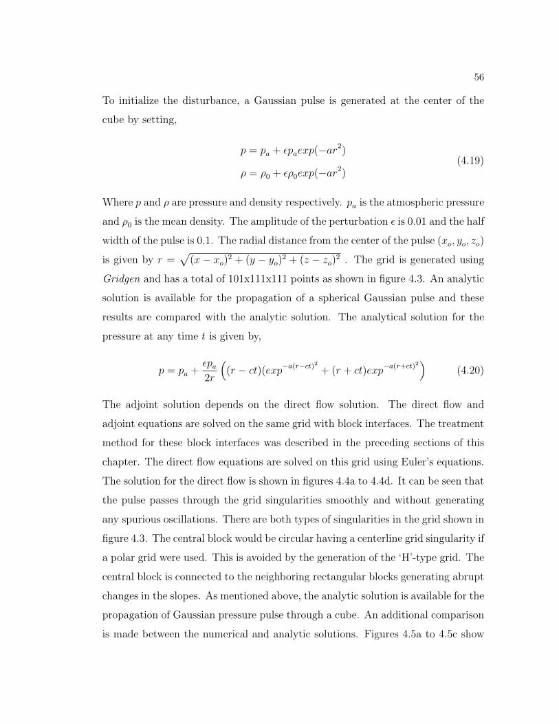
56
To initialize the disturbance, a Gaussian pulse is generated at the center of the
cube by setting,
p = pa + εpaexp(−ar2)
ρ = ρ0 + ερ0exp(−ar2)(4.19)
Where p and ρ are pressure and density respectively. pa is the atmospheric pressure
and ρ0 is the mean density. The amplitude of the perturbation ε is 0.01 and the half
width of the pulse is 0.1. The radial distance from the center of the pulse (xo, yo, zo)
is given by r =√
(x− xo)2 + (y − yo)2 + (z − zo)2 . The grid is generated using
Gridgen and has a total of 101x111x111 points as shown in figure 4.3. An analytic
solution is available for the propagation of a spherical Gaussian pulse and these
results are compared with the analytic solution. The analytical solution for the
pressure at any time t is given by,
p = pa +εpa2r
((r − ct)(exp−a(r−ct)2 + (r + ct)exp−a(r+ct)2
)(4.20)
The adjoint solution depends on the direct flow solution. The direct flow and
adjoint equations are solved on the same grid with block interfaces. The treatment
method for these block interfaces was described in the preceding sections of this
chapter. The direct flow equations are solved on this grid using Euler’s equations.
The solution for the direct flow is shown in figures 4.4a to 4.4d. It can be seen that
the pulse passes through the grid singularities smoothly and without generating
any spurious oscillations. There are both types of singularities in the grid shown in
figure 4.3. The central block would be circular having a centerline grid singularity if
a polar grid were used. This is avoided by the generation of the ‘H’-type grid. The
central block is connected to the neighboring rectangular blocks generating abrupt
changes in the slopes. As mentioned above, the analytic solution is available for the
propagation of Gaussian pressure pulse through a cube. An additional comparison
is made between the numerical and analytic solutions. Figures 4.5a to 4.5c show
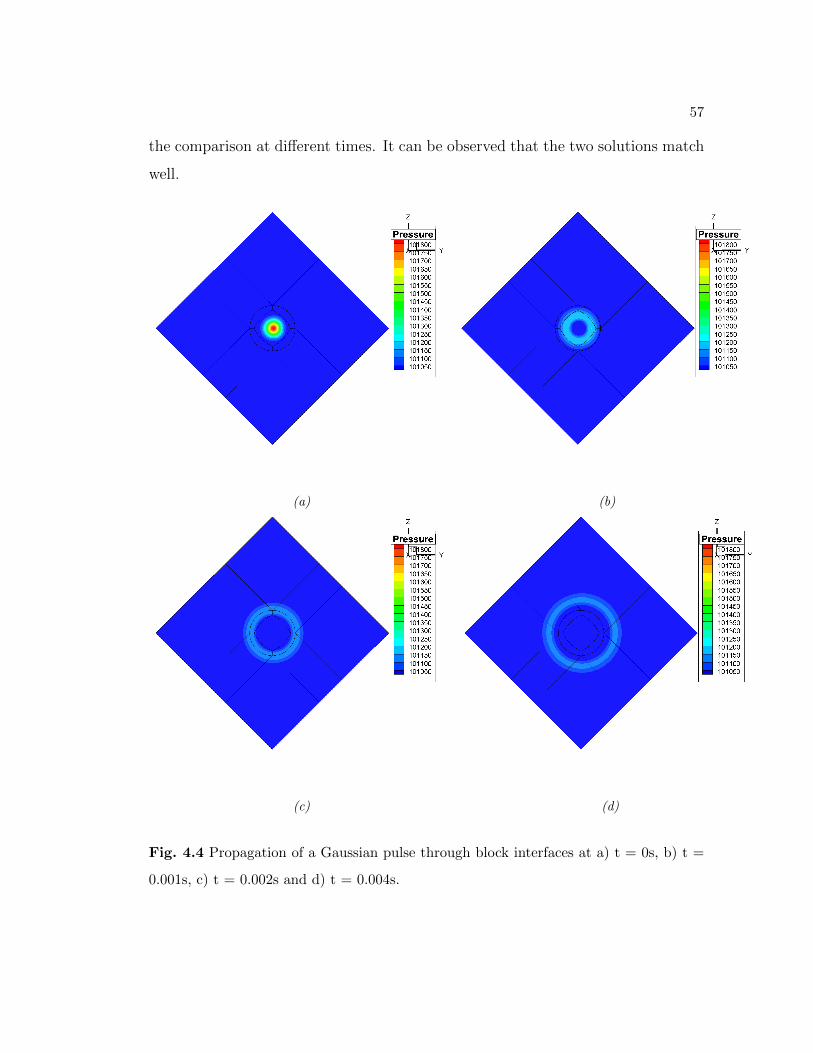
57
the comparison at different times. It can be observed that the two solutions match
well.
(a) (b)
(c) (d)
Fig. 4.4 Propagation of a Gaussian pulse through block interfaces at a) t = 0s, b) t =
0.001s, c) t = 0.002s and d) t = 0.004s.
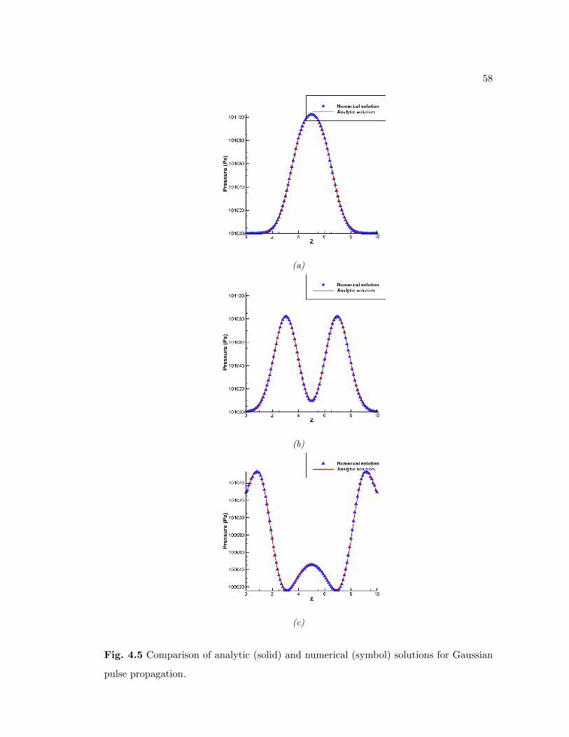
58
(a)
(b)
(c)
Fig. 4.5 Comparison of analytic (solid) and numerical (symbol) solutions for Gaussian
pulse propagation.

59
The second illustration describes the solution of the adjoint equations in a convergent-
divergent nozzle. Due to the potential singularity at the nozzle centerline, an ‘H’
shape grid is generated with 5 blocks in the axial direction. A cross section of the
nozzle is shown in figure 4.6. It can be observed that there are grid singularities
in the cross stream direction at the block interfaces. Figures 4.7a - 4.10b show the
steady state solution of the direct and adjoint equations. A similarity between the
adjoint and flow variables can be observed. But, the adjoint variables have oppo-
site trends than the direct flow variables. The inflow for the direct calculations
becomes the outflow for the adjoint variables and the outflow for the direct calcu-
lations becomes the inflow for the adjoint calculations. The regions of low pressure
become regions of high adjoint pressure. Similar traits can be observed in the
density and velocity behavior. These differences are also shown in the boundary
conditions. At the inflow, four direct boundary conditions are specified whereas
only one boundary condition is implemented for the adjoint variables. On the other
hand, at the outflow, one boundary condition is specified for the direct calculation
and four boundary conditions are specified for the adjoint solution. This reinforces
the notion that adjoint characteristics move in the opposite direction to the direct
characteristics, taking the information in the opposite direction. This is the reason
why adjoint variables can be used for the purpose of inverse optimization. They
bring feedback into the domain because of the characteristics moving in opposite
direction.

60
Fig. 4.6 The cross-section of the convergent-divergent nozzle with five blocks to avoid
centerline singularity.
(a) Direct pressure contours (b) Adjoint pressure contours
Fig. 4.7 The comparison of direct and adjoint pressure contours.

61
(a) Direct axial velocity contours (b) Adjoint axial velocity contours
Fig. 4.8 The comparison of direct and adjoint axial velocity contours.
(a) Direct cross-stream velocity contours (b) Adjoint cross-stream velocity contours
Fig. 4.9 The comparison of direct and adjoint cross-stream velocity contours.
(a) Direct density contours (b) Adjoint density contours
Fig. 4.10 The comparison of direct and adjoint density contours.

62
4.5 Conclusion
The adjoint method is a very efficient and computationally economic method to
achieve optimization when there are many design parameters in consideration. A
difficulty arises at the grid singularities when complex geometries are considered
and a multi-block grid topology is used. A method to treat the grid singularities for
complex multi-block grids has been described for the direct and adjoint equations.
The eigenvalue analysis of the adjoint equations reveals that adjoint characteristics
travel in the opposite direction to the physical characteristics. It has been shown
that this property can be used for the correction of residuals at the grid interfaces
according to the direction propagation of information.
4.6 Summary
A method to treat grid singularities for direct and adjoint calculations has been
discussed in this chapter. Grid singularities arise when there is an abrupt change
of the grid metrics. These singularities are treated by dividing the grid into multi-
ple blocks at the line of discontinuity. The line of discontinuity is considered as a
separate boundary and boundary conditions at this boundary are developed using
the characteristic form of the equations. It is shown that the method is effective
for all kinds of grid singularities with an example of the propagation of a Gaussian
pulse through the domain. The behavior of the adjoint and direct flow variables
is compared and it is shown that adjoint variables have characteristics opposite to
the direct flow variables.
The aim of this thesis to develop a method for the optimization of blowing at the
wall of a convergent-divergent nozzle to achieve a desired pressure distribution. It
will be shown that it is achievable with the use of two different approaches. The
first approach parameterizes the blowing velocity at a fixed region on the nozzle
wall and the optimum value of the parameters is found using the adjoint method.

63
The details of this approach are given in chapter 5. The second approach considers
the blowing velocity components as free design parameters, so the three blowing
velocity components at each grid point in the blowing region are considered as
independent design parameters. The sensitivity of the cost function with respect
to the blowing velocity components is then calculated using adjoint solution. The
details of this approach are given in chapter 6. Examples for both the approaches
are included in the respective chapters.

64
Chapter 5Parameterization of the Control
The general theory of the adjoint method was described in chapter 2. For a given
set of control parameters and constraints, an adjoint method is used to find the
value of the control parameters to minimize a cost or objective function. The goal of
this thesis is to demonstrate that the adjoint method can be used to find a blowing
distribution on a fixed region in the nozzle wall such that the pressure distribution
on the nozzle wall is close to a target pressure distribution. The blowing velocity
is the control parameter that is an unknown. There are several examples in the
literature of shape optimization using adjoint methods but there have been only
few uses of adjoint methods for the optimization of physical parameters such as
blowing velocity. Two approaches have been considered in this thesis. The first
approach is such that the blowing velocity is considered as a combination of basis
functions. This chapter describes the development of the adjoint equations with
the use of basis functions to determine the blowing velocity distribution. Two
examples, one with only one parameter to describe the blowing velocity and the
other with three parameters are given. The approach can be generalized for n
parameters. The blowing distribution g(x) is given by,
g(x) =N∑n=1
anfn(x) ;x ∈ Γa (5.1)

65
where an are the design parameters or control parameters, and fn(x) are the basis
functions. The basis functions are chosen such that they satisfy the constraints to
be followed by blowing velocity g(x). Γa is the region known as the ‘actuator’ where
blowing is to be implemented and N is the total number of design parameters. In
this chapter, it is shown that an adjoint method can be used to find the set of design
parameters an, such that the pressure distribution on the wall of a convergent-
divergent nozzle is close to a target distribution.
5.1 The Mathematical Development
The adjoint formulation used here is based on the boundary control theory de-
veloped by Collis [6] and Joslin [16]. Figure 5.1 shows a schematic of the nozzle
contour and the actuator and sensor regions. The sensor region Ωs is the region
where the pressure is matched (or in other words, the cost function is measured).
The actuator region Γa is the region where the blowing is implemented. Ω denotes
the full domain of computation, only half of the nozzle is considered because of
the symmetry about the nozzle centerline.
Fig. 5.1 Nozzle contour, sensor and actuator regions.

66
The present formulation is based on the invisicid Euler equations, the same ap-
proach can be used in the development for the Navier-Stokes equations and turbu-
lence models. The inviscid compressible Euler equations in conservative form are
given as,
∂U
∂t+∂F
∂x+∂G
∂y= 0 (5.2)
where,
U =
ρ
ρu
ρv
ρE
, F =
ρu
ρu2 + p
ρuv
ρuH
, G =
ρv
ρuv
ρv2 + p
ρvH
(5.3)
the system is closed with,
p = (γ − 1)ρ
(E − u2 + v2
2
)and H = E +
p
ρ(5.4)
The steady state problem is considered here and the time derivative term goes to
zero. But the time derivative term in the governing equations is retained since the
equations are marched in time to obtain the steady state solution. The adjoint
equations thus developed also include the time derivative term and artificial time
marching is used to obtain the steady state solution of adjoint equations. More
details on the steady state adjoint solution can be found in section 2.4. The
actuator region is considered as an inflow region where the blowing boundary
condition is implemented as an inflow boundary condition. More details of this
approach can be found in Collis et al. [6]. The number of boundary conditions
specified at a boundary is same as the number of incoming characteristics. In
the case of subsonic blowing, three characteristics travel into the domain whereas
one travels out of the domain. Hence three physical and one numerical boundary
condition have to be specified at the boundary. One boundary condition is that
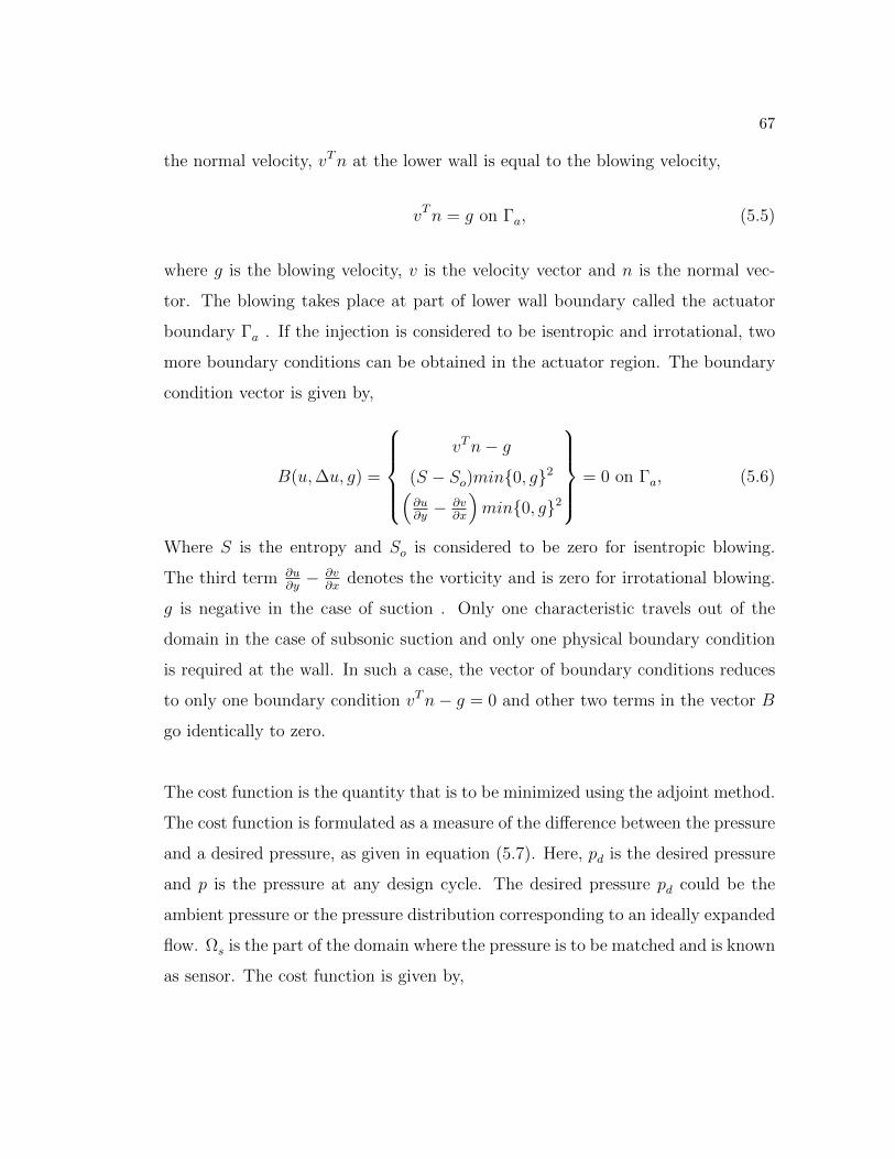
67
the normal velocity, vTn at the lower wall is equal to the blowing velocity,
vTn = g on Γa, (5.5)
where g is the blowing velocity, v is the velocity vector and n is the normal vec-
tor. The blowing takes place at part of lower wall boundary called the actuator
boundary Γa . If the injection is considered to be isentropic and irrotational, two
more boundary conditions can be obtained in the actuator region. The boundary
condition vector is given by,
B(u,∆u, g) =
vTn− g
(S − So)min0, g2(∂u∂y− ∂v
∂x
)min0, g2
= 0 on Γa, (5.6)
Where S is the entropy and So is considered to be zero for isentropic blowing.
The third term ∂u∂y− ∂v
∂xdenotes the vorticity and is zero for irrotational blowing.
g is negative in the case of suction . Only one characteristic travels out of the
domain in the case of subsonic suction and only one physical boundary condition
is required at the wall. In such a case, the vector of boundary conditions reduces
to only one boundary condition vTn− g = 0 and other two terms in the vector B
go identically to zero.
The cost function is the quantity that is to be minimized using the adjoint method.
The cost function is formulated as a measure of the difference between the pressure
and a desired pressure, as given in equation (5.7). Here, pd is the desired pressure
and p is the pressure at any design cycle. The desired pressure pd could be the
ambient pressure or the pressure distribution corresponding to an ideally expanded
flow. Ωs is the part of the domain where the pressure is to be matched and is known
as sensor. The cost function is given by,

68
J =1
2
∫Ωs
(p− pd)2 dΩ (5.7)
It is possible to apply additional constraints on the control by adding extra terms in
the cost function. Such constraints could be to make sure that the control remains
bounded and that there are no numerical fluctuations. The following constraints
are applied on the control g,
1. The magnitude of g should be a minimum to save power input.
2. g should vary smoothly.
that is,
g =dg
dx= 0 on ∂Γa (5.8)
where ∂Γa is the boundary of the region Γa. These constraints are applied by
adding penalty terms to the cost function. The modified cost function is given by,
J =α
2
∫Ωs
(p− pd)2 dΩ +β
2
∫Γa
(g2 +
dg
dx
2)dΓ (5.9)
The first additional penalty term makes sure that minimizing the cost function J
will minimize the magnitude of the control g and the second penalty term makes
sure that the control g should go smoothly to zero at the boundary ∂Γa of control
actuator g. α and β are the weighting parameters to control the relative contribu-
tion of two terms.
A Lagrange functional using the governing equations, control equations and the
modified cost function is formulated as,
L =α
2
∫Ωs
(p− pd)2 dΩ +β
2
∫Γa
(g2 +
dg
dx
2)dΓ +∫
Ω
λT[∂F
∂x+∂G
∂y
]dΩ +
∫Γa
λbTB(u,∆u, g)dΓ
(5.10)

69
Here, λ and λb are the adjoint variables or Lagrange multipliers corresponding to
the flow equations and the boundary conditions respectively.
The optimization of the cost function with respect to the constraints is the same
as making the Lagrangian functional stationary with respect to the variables. The
adjoint equations are obtained by setting ∂L∂uu′ = 0 for all u′,where u′ is the change
in the flow variables with respect to the change in the design parameters, and the
gradient of the cost function with respect to the control is calculated by,
∂J
∂gg′ =
∂L∂gg′ (5.11)
Here g is the control (blowing velocity), J is the cost function and L is the La-
grange functional. A prime on a quantity describes a fluctuation in that quantity.
The above holds true because the constraint equations are followed by the flow
variables and therefore the third and fourth terms are zero in equation (5.10).
The vectors of adjoint variables λ and boundary conditions λb are given by,
λ =λ1 λ2 λ3 λ4
T(5.12)
λb =λb1 λb2 λb3
T(5.13)
The gradient with respect to the design variables g is given by,
∂L∂gg′ = β
∫Γa
(gg′ +
∂g
∂x
∂g′
∂x
)∂Γ
+
∫Γa
λTbBg(u,∆u, g)g′ ∂Γ
(5.14)
Using the divergence theorem, this can be rearranged as,
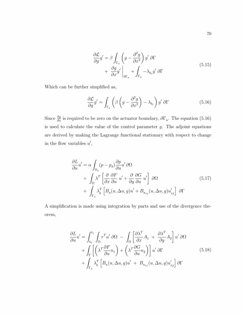
70
∂L∂gg′ = β
∫Γa
(g − ∂2g
∂x2
)g′ ∂Γ
+∂g
∂xg′∣∣∣∣∂Γa
+
∫Γa
−λb1g′ ∂Γ
(5.15)
Which can be further simplified as,
∂L∂gg′ =
∫Γa
(β
(g − ∂2g
∂x2
)− λb1
)g′ ∂Γ (5.16)
Since ∂g∂x
is required to be zero on the actuator boundary, ∂Γa. The equation (5.16)
is used to calculate the value of the control parameter g. The adjoint equations
are derived by making the Lagrange functional stationary with respect to change
in the flow variables u′,
∂L
∂uu′ = α
∫Ωs
(p− pd)∂p
∂uu′ ∂Ω
+
∫Ω
λT[∂
∂x
∂F
∂uu′ +
∂
∂y
∂G
∂uu′]∂Ω
+
∫Γa
λTb
[Bu(u,∆u, g)u′ +Buxj
(u,∆u, g)u′xj
]∂Γ
(5.17)
A simplification is made using integration by parts and use of the divergence the-
orem,
∂L
∂uu′ =
∫ t1
t0
∫Ω
rTu′ ∂Ω −∫
Ω
[∂λT
∂xA1 +
∂λT
∂yA2
]u′ ∂Ω
+
∫Γ
[(λT∂F
∂un1
)+
(λT∂G
∂un2
)]u′ ∂Γ
+
∫Γa
λTb
[Bu(u,∆u, g)u′ + Buxj
(u,∆u, g)u′xj
]∂Γ
(5.18)

71
where A1 = ∂F∂u
, A2 = ∂G∂u
and r = ∂p∂U
TKΩs. KΩs
is 1 when in Ωs and zero otherwise.
The adjoint equations as well as the boundary conditions can be summarized as,
AT1
∂λ
∂x+ AT
2
∂λ
∂y= r in Ω (5.19)
The adjoint boundary conditions are given by,
∑njB
T
uxjλb = 0 (5.20)
n1AT
1λ+ n2A
T
2λ+BT
uλb − ∂s
∑sjB
T
uxjλb = 0 (5.21)
where nj is the unit outward normal to the boundary and sj is the tangential
vector on the boundary.
5.2 Optimization with Parameterization of Blow-
ing
The goal of this chapter is to demonstrate that the above approach can be used
to find a blowing distribution on the nozzle wall such that the pressure in a fixed
region matches well with the target pressure. The blowing is dependent on a
number of design parameters. The formulation and implementation of this method
is complex and nontrivial. To simplify the problem, the blowing is incorporated on
a limited section of the nozzle wall and two-dimensional calculations are performed
for the interior of nozzle. It is shown that moving the shock towards the exit of
the nozzle is possible with the use of blowing. Two examples are given. The first
example has a Gaussian blowing distribution and the amplitude of this Gaussian
is considered as the control parameter. The optimum value of the amplitude is
found using the adjoint approach. The second example considers the blowing
distribution as a combination of three trigonometric functions. The coefficients of

72
these three functions are considered as control parameters. The optimum values of
these parameters are found using the adjoint approach as described in this chapter.
As a simple example of the design process a contoured nozzle with a simple geom-
etry is considered. The nozzle contour is given by,
y = 1.75− 3αcos[(0.2x− 1)π] for 0 ≤ x ≤ 5
y = 1.25− 3αcos[(0.2x− 1)π] for 5 ≤ x ≤ 10(5.22)
where the value of α is 0.25. A Gaussian distribution with the amplitude vb
is considered for the blowing velocity at the wall. The blowing distribution is
described as,
g(x) = vb exp
− x− (x1+x2)2
2
[(x− x1)2(x− x2)2]
for x1 ≤ x ≤ x2 (5.23)
Note that this distribution follows the condition (5.8) and the value of blowing
velocity g goes to zero at the actuator boundaries x1 and x2. A positive g means
that fluid is injected into the flow whereas a negative g means suction out of the
domain. The nozzle pressure ratio is kept constant so that the operating conditions
remain the same for all the cases. The value of nozzle pressure ratio is 1.5 for the
results presented here. The nozzle contour geometry has been kept fixed and is
given by equation (5.22). The goal is to find an appropriate blowing rate that will
remove the shock from the nozzle interior without changing the nozzle geometry
or operating conditions. The cost function is given by equation (5.7), where the
desired pressure is found for a known value of the amplitude vb. The desired
pressure distribution is first found for vb = 60 m/s. The cost function is measured
inside a fixed region of the nozzle as shown in figure 5.1. Figure 5.2 shows the
changes in the flow as the amplitude of blowing velocity is varied. The shock
location and pressure contours change as the value of vb is varied. The shock
moves towards the nozzle exit as the rate of blowing is increased. Since only the
interior of the nozzle has been considered for this calculation, complete removal of

73
the shock is not possible but the shock is pushed to the nozzle exit. The pressure
corresponding to vb = 60.0 m/s is taken as the desired pressure. The goal is to
reach to the desired value of pressure using an adjoint optimization approach. The
change in blowing velocity amplitude with design cycles is shown in figure 5.3. The
value of the amplitude changes from an initial value of zero to a value of 59.032 m/s
in 5 design cycles. The value of vb changes more rapidly in the initial design cycles
and changes at a slower rate as it approaches the desired value. It then begins to
fluctuate around this value. The decay in the cost function is shown in figure 5.4,
the cost function decays almost linearly whereas the blowing amplitude changes in
a non-linear fashion. As the pressure distribution gets close to the desired pressure,
the amplitude of blowing vb also moves towards the desired blowing. It will be seen
in the next chapter that when there is more than one control parameter, in some
cases the adjoint approach finds a new value of the control parameters, but the
pressure distribution thus found is always close to the target distribution.

74
Fig. 5.2 The variation in pressure contours and streamlines, in the divergent section of
the nozzle, as the amplitude of the blowing velocity vb is varied to 0, 10, 30 and 60 m/s.
Fig. 5.3 Variation of the amplitude of the blowing vb in m/s with design cycles.

75
Fig. 5.4 Decay of the cost function in Pa2 with design cycle.
The first example, as shown above, demonstrates that the adjoint method can be
used to find the blowing amplitude on the nozzle wall. The method can be used to
find a pressure distribution corresponding to a known blowing distribution, where
the blowing distribution is dependent only on one parameter. The second example
considered is more general example than this. A blowing distribution based on
several control parameters is considered and the optimum solution is not known.
An adjoint method is used to find that blowing distribution that removes the
shock from inside the nozzle. The blowing distribution has been considered as a
combination of trigonometric basis functions that follow the condition (5.8). The
sensitivity of the cost function with respect to these control parameters can be
found using the adjoint method. The generalized blowing distribution g is given
by,
g(x) =1
2
N∑n=1
an1− cos[(2n− 1)3π(x− x1)/2(x2 − x1)] x ∈ [x1, x2] (5.24)

76
g′(x) =1
2
N∑n=1
an(2n− 1)3π
2(x2 − x1)sin[(2n− 1)3π(x− x1)/2(x2 − x1)] (5.25)
Here an are the control parameters. The total number of design parameters, N
is taken to be 3 for simplicity but a larger value of N could be considered with-
out much difference in the computational cost. In this case the cost function is
calculated in a region near the lower wall and the desired pressure is taken to be
the ambient pressure. The goal is to achieve a pressure distribution in the sensor
region, that is as close to the ambient pressure as possible, using blowing at the
lower wall. The cost function is formulated as equation (5.7), where pd is consid-
ered to be ambient pressure pa.
The nozzle pressure ratio has been kept constant as before and the geometry is
fixed to the initial geometry as shown in figure 5.22. There is no blowing for the
first design cycle. The region of observation or sensor can be chosen as any region
in the nozzle interior domain or on the boundaries. This region is shown by the box
in figure 5.5. This region has been chosen based on the initial flow field such that
it captures the shock. The sensor region extends in the axial direction between
x/D = 8.0 to x/D = 9.1 and in the transverse direction it goes from y/D = 0.5 to
y/D = 1.0, whereD is the nozzle throat diameter. The sensor region approximately
spans 8.3% area of the total nozzle domain. The shock removal inside the nozzle
was achieved by using the blowing on the wall with a blowing distribution given by
equation (5.24). There is no blowing in the first design cycle. Figure 5.5 shows the
pressure contours after different numbers of design cycles. It takes 4 design cycles
to obtain the blowing distribution that shows no shock inside the nozzle. The
normalized cost function dropped from a value of 5.06 to 2.03. Then it increases
and then keeps fluctuating about the minimum value. The fluctuations in the cost
function are significant. But, this can be circumvented by the multiplication of a
relaxation coefficient in the updating of the control parameters.

77
Fig. 5.5 Removal of shock with adjoint design cycles. The sensor region is shown as a
box in the diverging section of the nozzle.
5.3 Conclusion
Blowing at the nozzle wall can be used to change the pressure distribution inside
the nozzle. It is possible to use an adjoint approach to find the blowing velocity
distribution such that the pressure inside the nozzle matches well with the desired
pressure. The blowing velocity can be written as a combination of multiple pa-
rameters and/or basis functions. The basis functions are chosen such that they
follow the constraints required of the blowing velocity. The coefficients of the basis
functions are considered as control parameters. An adjoint approach is developed
such that the blowing region is considered as an inflow boundary and the gradients
of the cost function with respect to the coefficients of the basis functions are found

78
using the adjoint method. These gradients are then used to calculate the new
values of the coefficients. In the first example, where the blowing velocity distribu-
tion is Gaussian in shape, the amplitude of the blowing velocity is achieved within
an error of 1.6% in 5 design cycles. In the second example, where the blowing is
described in terms of three control parameters, it is shown that moving the shock
to the nozzle exit is possible by using this approach. In the case where an external
domain is included in the computation, this approach can be used to move the
shock out of the nozzle which can help in reducing the shock associated noise.
5.4 Summary
This chapter describes the development and implementation of an adjoint method
to optimize the blowing in a fixed region on a nozzle wall. The blowing has been
considered to be a sum of the products of design parameters and basis functions.
It is shown that the adjoint method can be used to minimize the cost function
that is defined in a region inside the nozzle. For most practical cases it is not
necessarily possible to achieve a blowing distribution thus described. It also lim-
its the solution space to those blowing distributions that can be written in the
given form. These issues are addressed in the next chapter where a free form of
the blowing distribution is considered. The blowing velocity at each grid point
inside the actuator region is considered to be an independent design parameter.
All components of velocity are considered as independent variables. The blowing
distribution thus found can be used to determine the angle of injection because
all three components of the velocity are considered separately. A two-dimensional
method is first developed and is later extended to three-dimensions. More details
on how the desired pressure is calculated and the blowing distribution is found
using the adjoint method are given in the next chapter.

79
Chapter 6Adjoint Control of Nozzle Flow withSurface Blowing
6.1 Introduction
This chapter describes how the adjoint method can be used to find the values of
control parameters that describe the blowing distribution on the nozzle wall to
minimize a given cost function. In this chapter a free form of blowing has been
considered as the control. It is not necessarily possible to physically achieve a
blowing distribution that is given by a set of basis functions. So, in this chapter,
all velocity components at each grid point in the actuator region are considered
as independent parameters. The relative values of the components of the blowing
velocity can be used to determine the angle of injection at the nozzle wall. This
chapter provides the tools to optimize the blowing on the nozzle wall.
The mathematical development of the adjoint equations when the control param-
eters are the blowing velocity components, differs from that given in the previous
chapter, when the control parameters are the coefficients of given basis functions of
the normal blowing velocity. A brief introduction of the mathematical development
is given first in this chapter. Because of the complexity of the adjoint equations,
a two-dimensional case is first considered. Two examples for the two dimensional
case are given. The first example demonstrates that the adjoint method can be

80
used to find an arbitrary blowing distribution such that the pressure at the nozzle
wall matches with the pressure corresponding to a known blowing distribution.
The second example shows how to achieve ideally-expanded flow from a nozzle
that is operating at off-design conditions. Then three-dimensional calculations are
performed for both the nozzle internal and external flows. First, internal flow re-
sults for the blowing optimization on the nozzle wall are given when the pressure is
to be matched with a desired pressure distribution on the nozzle wall. The second
example also includes the nozzle external flow and the optimization technique for
blowing when the external flow is included.
6.2 The Mathematical Development with Wall
Blowing Control
This section describes the development of the adjoint equations and boundary
conditions and the determination of the sensitivity of the cost function to the
design parameters. The present analysis and computations are based on the Euler
equations. The same general approach can be used for the Navier-Stokes equations
and for turbulence model equations. The reason for choosing the inviscid model
is the simplicity of development and implementation that is offers. This would
result in a loss of flow physics in the boundary layer region but this is neglected
for the present analysis since the purpose of this analysis is to demonstrate the
methodology of adjoint and not to capture the fine details of flow behavior. A
more sophisticated analysis provides the scope of the future work.
The three-dimensional, compressible, inviscid governing equations in conservative
form can be written as,
∂U
∂t+∂Fi∂xi
= 0, (6.1)
Here a repeated index implies a summation. The flux vector Fi is given by,

81
Fi = mi,miu1 + pδi1,miu2 + pδi2,miu3 + pδi3,miHT , (6.2)
And the vector of conserved variables, U, is given by,
U = ρ,m1,m2,m3, eT , (6.3)
where,
m1 = ρu1 , m2 = ρu2, m3 = ρu3, and e = ρEn (6.4)
The Kronecker delta δij is 1 when i = j and 0 otherwise. u1, u2 and u3 are the
velocity components in the x1, x2 and x3 directions respectively, En is the internal
energy, H is the enthalpy, ρ is the density and p is the static pressure. The system
is closed by the following equations for a calorically perfect gas,
H = (e+ p)/ρ, and p = (γ − 1)
[e− (mimi)
2ρ
]. (6.5)
The boundary conditions at the nozzle inflow, outflow, far field and wall are given
by,
p = pa for subsonic outflow on Γo
Po = constant and To = constant on Γi
uN = 0 on Γw
ui = ubqi on Γa
(6.6)
where, Γo is the outflow boundary, Γi is the inflow boundary, Γw is the wall bound-
ary and Γa is the actuator boundary where blowing is applied. Po and To are
respectively the total pressure and total temperature at the nozzle inlet, uN is the
wall normal velocity, pa is the ambient pressure and ubqi is the blowing velocity at

82
the qth node in the ith direction.
Together, the governing equations can be written as,
R = 0 (6.7)
The changes in R due to changes in the flow variables U are given by,
δR =∂(δU)
∂t+∂(δFi)
∂xi, (6.8)
where,
δFi =∂Fi∂U
δU (6.9)
and,
δU =∂U
∂UδU = PδU (6.10)
where, U is the vector of primitive variables given by,
U = p, u1, u1, u3, TT , (6.11)
The cost function to be minimized depends on the difference between the pressure
at any design cycle and a desired pressure on a sensor where the sensor is the
region where the cost function is measured. The sensor could either be a section of
the nozzle wall or a region in the flow domain. In the former case the cost function
is given by,
J =α
2
∫t
∫Γs
(p− pd)2 dΓdt, (6.12)
where Γs is the sensor region.The time derivative terms have been retained in the
formulation as the steady state direct and adjoint solutions are obtained using time
marching.

83
Using the cost function and the flow equations a Lagrangian functional L can be
constructed as,
L = J +
∫t
∫Ω
QTR dΩdt, (6.13)
where Ω is the computational domain surrounded by the boundary Γ. Q is the
vector of adjoint variables and is given by,
Q = q1, q2, q3, q4, q5T . (6.14)
The perturbation of the Lagrangian functional with respect to the design param-
eters is given by,
δL = δJ +
∫t
∫Ω
QT δRdΩdt. (6.15)
δR is given by equation (6.8), so that,
δL = δJ +
∫t
∫Ω
QT
[∂(δU)
∂t+∂(δFi)
∂xi
]dΩdt (6.16)
From equation (6.10),
δL = δJ +
∫t
∫Ω
QT
∂(δU)
∂t+∂ [(∂Fi/∂U) δU]
∂xi
dΩdt (6.17)
Integration by parts and use of the divergence theorem yields,
δL = δJ +
[∫Ω
QT δU
]t2t1
+
∫t
∫Γ
QT ∂δFi∂U
niδUdΓdt
−∫t
∫Ω
(∂QT
∂t+∂QT
∂xi
∂Fi∂U
)δUdΩdt
(6.18)
Equation (6.18) has three terms that have separate meanings. The concept behind
the adjoint approach is to find the gradients of the cost function with respect to the
design variables, without having to calculate the change in the flow variables δU.

84
Hence the integrand in the last term of equation (6.18) is set to zero everywhere in
the flow domain. This results in a set of equations that are known as the “adjoint
equations”. The first and third terms on the right hand side of equation (6.18)
represent boundary terms and are discussed in detail in the next section. The
second term is the time condition term and the adjoint variables are set to zero at
the initial adjoint time, t2, that is,
Qt=t2 = 0. (6.19)
This condition is used as the initial condition for the adjoint solution.
The adjoint equations are developed such that the sensitivity of the cost function
with respect to the control parameters is independent of the sensitivity of the
flow variables with respect to the design variables. In order to achieve this, the
integrands in equation (6.18) are set to zero in the volume integrals. So, the adjoint
equations are given by,
∂Q
∂t+∂Fi∂U
T ∂Q
∂xi= 0 (6.20)
or,∂Q
∂t+ Ai
T ∂Q
∂xi= 0 (6.21)
with Ai = ∂Fi∂U
. After further simplification, the adjoint equations are found to be
given by,
∂q1
∂t= −(γ − 1)q2(
∂q2
∂x1
+∂q3
∂x2
∂q4
∂x3
) + u1ui∂q2
∂xi
+ u2ui∂q3
∂xi+ u3ui
∂q4
∂xi
−(− c2
γ − 1+ (γ − 2)q2
)ui∂q5
∂xi,
(6.22)

85
∂q2
∂t= − ∂q1
∂x1
− (3− γ)u1
∂q2
∂x1
− u2
(∂q2
∂x2
+∂q3
∂x1
)− u3
(∂q2
∂x3
+∂q4
∂x1
)+ (γ − 1)u1
(∂q3
∂x2
+∂q4
∂x3
+ ui∂q5
∂xi
)− H
∂q5
∂x1
,
(6.23)
∂q3
∂t= − ∂q1
∂x2
− (3− γ)u2
∂q3
∂x2
− u3
(∂q3
∂x3
+∂q4
∂x2
)− u1
(∂q3
∂x1
+∂q2
∂x2
)+ (γ − 1)u2
(∂q4
∂x3
+∂q2
∂x1
+ ui∂q5
∂xi
)−H ∂q5
∂x2
,
(6.24)
∂q4
∂t= − ∂q1
∂x3
− (3− γ)u3
∂q4
∂x3
− u1
(∂q4
∂x1
+∂q2
∂x3
)− u2
(∂q4
∂x2
+∂q3
∂x3
)+ (γ − 1)u3
(∂q2
∂x1
+∂q3
∂x2
+ ui∂q5
∂xi
)−H ∂q5
∂x3
,
(6.25)
and,∂q5
∂t= −(γ − 1)
(∂q2
∂x1
+∂q3
∂x2
+∂q4
∂x3
)− γui
∂q5
∂xi. (6.26)
Here, q2 = uiui/2 and c is the speed of sound, given by, c2 = (γp)/ρ. H is the
enthalpy, given by q2 + c2
γ−1. The time derivatives have been retained for the arti-
ficial time marching.
Equations (6.22)– (6.26) are the adjoint equations. The adjoint equations are
homogeneous linear equations. The boundary conditions on the adjoint variables
depend on the direct boundary conditions. The boundary conditions for the adjoint
variables are developed in the following section.

86
6.3 Boundary Conditions
The adjoint boundary conditions play a crucial role in the accuracy and stability
of the adjoint solution as in any other problem in numerical fluid mechanics. The
adjoint boundary conditions are related to the direct flow boundary conditions and
are developed in conjunction with the direct flow boundary condition.
The direct flow boundary conditions given by equation (6.6) are implemented ei-
ther in terms of the derivatives of the flow variables (Neumann conditions) or the
values of the flow variables (Dirichlet conditions). In both cases, the information
about the flow variables is obtained at the boundaries. This information can be
transformed to provide the change in the flow variables, δU at the boundaries. The
value of δU at the boundaries is then considered in the adjoint boundary terms
to provide information about the adjoint variables at the respective boundaries.
Thus, the adjoint boundary conditions are developed based on the change in direct
flow variables δU at the boundaries. The details are given in the following section.
The Simplification of the Adjoint Boundary Integrand
The boundary integral terms in the expression for δL are given by,
δL = δJ +
∫t
∫Γ
QT ∂Fi∂U
niδUdΓdt (6.27)
The cost function J is given by equation (6.12). Taking the perturbation of this
equation yields,
δJ = α
∫t
∫Γs
(p− pd)δp dΓdt, (6.28)
The integrand in the boundary terms can be written as,

87
QT ∂Fi∂U
niδU = QT ∂Fi∂U
ni∂U
∂UδU (6.29)
where U and U are the vectors of conserved and primitive flow variables respec-
tively given by,
U = ρ, ρu1, ρu2, ρu3, ρEnT ,
U = p, u1, u2, u3, TT .(6.30)
The transformation matrix of conversion between the primitive and conservative
variables, P is defined by,
P =∂U
∂U. (6.31)
Then the integrand of the boundary terms on the right hand side of the equation
(6.27) can be written as,
QT ∂Fi∂U
PniδU =(P δp+ Uiδui + T δT
). (6.32)
The integrand of the boundary term in the new expression for δL is given by,
Boundary Integrand =(α(p− pd)k + P
)δp+ Uiδui + T δT (6.33)
Here k is introduced to generalize the form of boundary conditions and is given
by,
k = 0 on Γ ∩ Γs,
k = 1 on Γs.(6.34)
The terms with an overbar represent the coefficients of the respective flow variable
perturbations. The coefficients in equation (6.33) can be simplified using the flow
equations and are given by,

88
P =uNRT
(u · q + q1 +Hq5) + qN , (6.35)
T =−pRT 2
uN (u · q + q1 +Hq5) +p
T
γ
γ − 1q5uN , (6.36)
U1 =p
RT(q1n1 + u1uNq5 +Hq5n1 + 2u1q2n1 + u2(q2n2 + q3n1) + u3(q2n3 + q4n1)) .
(6.37)
Similarly,
U2 =p
RT(q1n2 + u2uNq5 +Hq5n2 + 2u2q3n2 + u3(q3n3 + q4n2) + u1(q3n1 + q2n2)) ,
(6.38)
and,
U3 =p
RT(q1n3 + u3uNq5 +Hq5n3 + 2u3q4n3 + u1(q4n1 + q2n3) + u2(q4n2 + q3n3)) .
(6.39)
Here uN and qN are the wall normal direct and adjoint velocities given by,
uN = u1n1 + u2n2 + u3n3, (6.40)
and,
qN = q2n1 + q3n2 + q4n3. (6.41)
where n1, n2 and n3 are the components of the outward normal to the wall.
The adjoint equations are developed such that the requirement to calculate the
change in the flow variables δU is circumvented by making the coefficients of δU
vanish whenever possible. The adjoint boundary conditions are developed using
the same approach. The boundary integrals can be eliminated by setting the
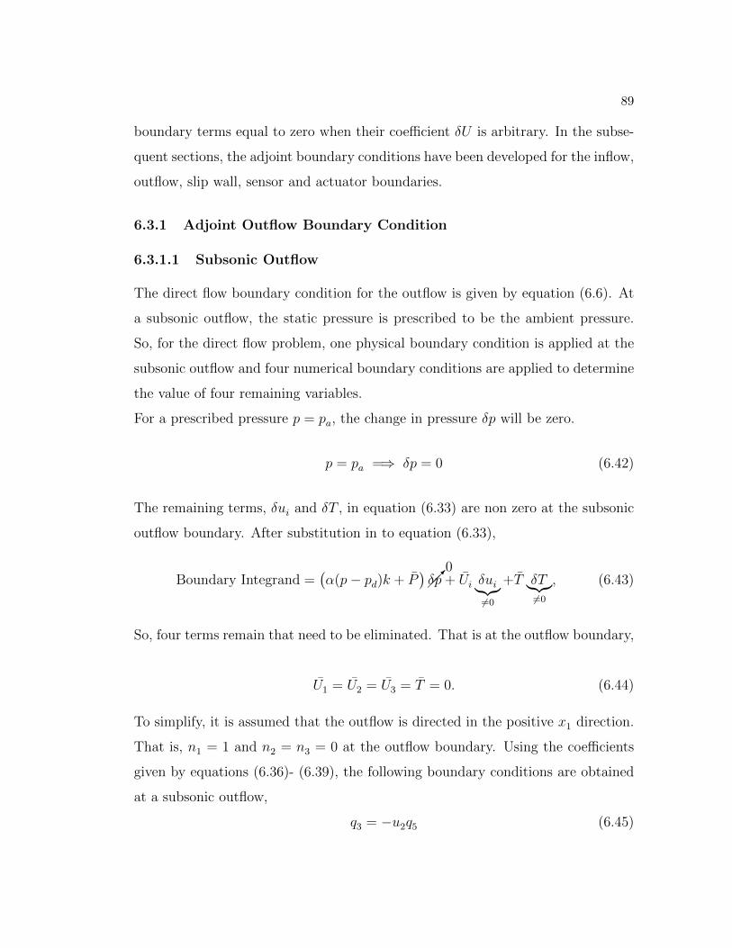
89
boundary terms equal to zero when their coefficient δU is arbitrary. In the subse-
quent sections, the adjoint boundary conditions have been developed for the inflow,
outflow, slip wall, sensor and actuator boundaries.
6.3.1 Adjoint Outflow Boundary Condition
6.3.1.1 Subsonic Outflow
The direct flow boundary condition for the outflow is given by equation (6.6). At
a subsonic outflow, the static pressure is prescribed to be the ambient pressure.
So, for the direct flow problem, one physical boundary condition is applied at the
subsonic outflow and four numerical boundary conditions are applied to determine
the value of four remaining variables.
For a prescribed pressure p = pa, the change in pressure δp will be zero.
p = pa =⇒ δp = 0 (6.42)
The remaining terms, δui and δT , in equation (6.33) are non zero at the subsonic
outflow boundary. After substitution in to equation (6.33),
Boundary Integrand =(α(p− pd)k + P
)
0δp+ Ui δui︸︷︷︸
6=0
+T δT︸︷︷︸6=0
, (6.43)
So, four terms remain that need to be eliminated. That is at the outflow boundary,
U1 = U2 = U3 = T = 0. (6.44)
To simplify, it is assumed that the outflow is directed in the positive x1 direction.
That is, n1 = 1 and n2 = n3 = 0 at the outflow boundary. Using the coefficients
given by equations (6.36)- (6.39), the following boundary conditions are obtained
at a subsonic outflow,
q3 = −u2q5 (6.45)

90
q4 = −u3q5 (6.46)
q2 = − 1
u1
(u2
1+
c2
γ − 1
)q5 (6.47)
q1 =
(q2 +
c2
γ − 1
)q5 (6.48)
Equations (6.45)- (6.48) are the boundary conditions for the adjoint outflow. At
the subsonic outflow one adjoint variable is extrapolated from the interior of the
domain and the four boundary conditions given by (6.45) to (6.48) are applied to
calculate the values of the remaining four adjoint variables at the outflow.
6.3.1.2 Supersonic outflow
At a supersonic outlet, none of the flow quantities is specified for the direct flow
and all of the variables are computed from the interior of the domain. Thus, at
the outflow,
δp 6= 0, δui 6= 0, δT 6= 0. (6.49)
So the coefficients of δui, δp and δT in equation (6.33) must vanish at the outlet.
That is,
Boundary Integrand =(α(p− pd)k + P
)δp︸︷︷︸6=0
+Ui δui︸︷︷︸6=0
+T δT︸︷︷︸6=0
, (6.50)
So, at a supersonic outflow,
U1 = U2 = U3 = T = P = 0. (6.51)
Five boundary conditions are obtained from these relationships. On simplification,
the equations reduce to,
q3 = −u2q5 (6.52)
q4 = −u3q5 (6.53)

91
q2 = − 1
u1
(u2
1+
c2
γ − 1
)q5 (6.54)
q1 =
(q2 +
c2
γ − 1
)q5 (6.55)
and
q1 + q2u1 + q3u2 + q4u3 + q5
uiui2
= 0. (6.56)
Equations (6.52) - (6.56) can be used to solve for q1, q2, q3, q4, q5T at a supersonic
outflow.
6.3.2 Adjoint Inflow Boundary Condition
The boundary condition at the nozzle inlet for the direct problem is given by
equation (6.6). The total pressure and total temperature are specified at the
nozzle inlet. The flow direction at the nozzle inlet is also specified. For simplicity,
it is assumed that the nozzle inlet surface is normal to the x1 direction. That is,
n1 = −1 and n2 = n3 = 0 at the inlet. An inlet in any general direction can be
considered in the same way.
For the direct flow,
Po = constant ;To = constant, u2 = u3 = 0, (6.57)
at the nozzle inflow. Then, at the inflow,
δPo = 0 ; δTo = 0 ; δu2 = δu3 = 0 (6.58)
The isentropic flow relations are given by,
To = T
(1 +
γ − 1
2
u21
γRT
)and Po = p
(1 +
γ − 1
2
u21
γRT
) γγ−1
. (6.59)

92
Finding the change in these equations and using equations (6.58), (6.59) the rela-
tions between δT , δp and δu1 can be found. These relations are given by,
δT =γ − 1
γRu1δu1. (6.60)
Similarly,
δp = −pu1
RTδu1. (6.61)
Substituting these into the boundary integrand (6.33) yields,
Boundary Integrand =(α(p− pd)k + P
)δp︸︷︷︸
f(δu1)
+U1 δu1︸︷︷︸6=0
+U2>
0δu2 + U3
>0
δu3 + T δT︸︷︷︸f(δu1)
,
(6.62)
using equations (6.60) and (6.61), the coefficients of δT and δp can be combined to
make one coefficient of δu1. u1 is arbitrary at the inflow boundary, so the coefficient
of δu1 must vanish at the inflow. This results in one adjoint boundary condition
at the inflow, given by,
q2 = − 1
u1
[q1 +
(q2 +
c2
γ − 1
)q5
](6.63)
At the adjoint inflow, four numerical boundary conditions are applied to the ad-
joint variables q1, q3, q4, q5 and the values are extrapolated from the interior of the
domain. So, one adjoint boundary condition, given by equation (6.63), is applied
to calculate q2 at the inflow boundary.
6.3.3 Adjoint Slip Wall Boundary Condition
At a slip wall, for direct flow, there is no flow penetration (except at the actuator
boundary). The wall boundary condition for the direct flow problem is given by
zero wall normal velocity,
uN = 0. (6.64)

93
This can be written as,
δu1n1 + δu2n2 + δu3n3 = 0. (6.65)
For an adiabatic wall, there is no specification of p or T on the wall, therefore δp
and δT are arbitrary on the wall. Considering the adjoint boundary integrand :
Boundary Integrand =(α(p− pd)k + P
)δp︸︷︷︸6=0
+U1 δu1︸︷︷︸6=0
+U2 δu2︸︷︷︸6=0
+U3 δu3︸︷︷︸6=0
+T δT︸︷︷︸6=0
,
(6.66)
The coefficients of δT and δp are required to vanish on a slip wall because no
information is given about δT and δp. That is,
T = P = 0 (6.67)
The coefficients of δui are not individually equated to zero because of the known
condition given by (6.65). Using equation (6.35) and (6.65), a single adjoint
boundary condition is obtained at the slip wall,
q2n1 + q3n2 + q4n3 = qN = 0, (6.68)
where qN is the wall normal adjoint velocity. Using the wall normal adjoint and
direct velocities equal to zero, equation (6.64) and (6.68), the equation for T and
P (6.67) is satisfied automatically. Thus equation (6.68) provides the only bound-
ary condition required at a slip wall.
6.3.4 Sensor Boundary Condition
In the present formulation, the sensor is a region on the wall boundary. The wall
boundary condition must be modified to account for the sensor region. In gen-
eral, the sensor could be any part of the domain. If the sensor region is inside
the computational domain, the cost function term appears as a source term in the

94
equations. If the sensor were at any other boundary, the cost function term would
appear in the respective boundary condition.
The general expression for the wall boundary conditions is still applicable at the
part of the wall which is defined as sensor. The parameter k, as defined earlier by
equation (6.34), is non-zero at the sensor and adds an extra term to the boundary
condition. At the sensor,
P + α(p− pd) = 0 (6.69)
Simplification of this equation yields,
qN + α(p− pd) = 0 (6.70)
The wall normal adjoint velocity in the sensor region is non-zero and is given by
the difference between the pressure at any design cycle and the desired pressure.
6.3.5 Actuator Boundary Condition
The actuator is the part of boundary where control (in this case, the injection or
blowing) is implemented. The boundary condition on the actuator for the direct
flow solution is different from than that on a solid wall. So the boundary condition
for the adjoint calculation on the actuator is also different from that of the solid
wall. The control, or actuator boundary, consists of blowing velocities at different
nodes that are each considered as independent control variables. Each grid point in
the actuator region is considered as one node. In general, all three components of
the blowing velocities at these nodes are considered as separate control parameters.
So, if the number of nodes in the actuator region is q, the total number of control or
design parameters N for a three-dimensional problem will be 3q. Since all of these
control parameters can change independently, the sensitivity of the cost function

95
with respect to each of these control parameters must be calculated. Therefore a
total of 3q sensitivities have to be calculated.
The boundary conditions for the direct flow calculation on the actuator are given
by,
u1 = ub1 , u2 = ub2 , u3 = ub3 . (6.71)
Where the subscript ‘b′ expresses a blowing velocity. The boundary conditions on
node ‘q’ can be written as,
u1 = ubq1 , u2 = ubq2 , u3 = ubq3 . (6.72)
The perturbation in these quantities with respect to the blowing velocities is either
1 or 0 depending on which component of the blowing velocity is considered. That
is, at the actuator node ‘q’, from Equation (6.72),
δuqiδubqj
= δij, (6.73)
where δij is Kronecker delta and has been defined earlier. Consider the boundary
term in the expression for δL, given in equation (6.33),
Boundary Integrand =(α(p− pd)k + P
)δp+ Uiδui + T δT. (6.74)
The coefficients of δui in the above expression remain non-zero because the δui
are non-zero in the actuator region. Hence, the boundary conditions in this re-
gion are obtained from the first and last terms (the coefficients of δT and δp), in
equation (6.74). They are given by,
P = T = 0, (6.75)

96
After simplification, the boundary conditions on the actuator are then given by,
q5 = − γ
(γ − 1)
qNuN
(6.76)
q1 = −(q2ubq1 + q3ubq2 + q4ubq3) +γ − 1
γ
ubqiubqi2
qNuN
(6.77)
Here, uN and qN are the direct and adjoint wall normal velocities, and are given
by,
uN = uini (6.78)
qN = q2n1 + q3n2 + q4n3 (6.79)
The remaining non zero terms on the actuator add to the gradient of the cost
function with respect to the actuator velocity components. These terms are given
by,
δLδubqi
= Ui for i = 1, 2, 3, (6.80)
where ui is the velocity component in the ith direction.
Equation (6.80) is used to calculate the sensitivity of the cost function to the
blowing velocities at the qth node.
6.4 The Optimization Procedure
The gradients of the cost function are calculated as described above. The details
of the adjoint optimization cycle are given in section 2.2. A gradient based search
method can then be incorporated to find the local optimum. A Newton’s search
method is used here to find the next set of design variables. The new vector of
blowing velocities is given by,
unewbi
= uoldbi− Jold
δL/δubi(6.81)

97
6.5 Results and Discussion
The method used to develop the adjoint equations and adjoint variables to calcu-
late the sensitivities of a defined cost function with respect to the blowing velocities
was described in the previous section. In this section, examples of the use of this
approach are given. Two and three-dimensional calculations are performed for
several cases. The first case is a two-dimensional example that recovers a pressure
distribution on the nozzle wall that is calculated using a known blowing distri-
bution. The second example is set such that two-dimensional ideally expanded
flow is achieved inside a nozzle when the nozzle is operating at off design con-
dition. The blowing velocities at the nozzle wall are used as control parameters
and the adjoint approach is used to optimize their values. Three-dimensional cal-
culations are then performed for both nozzle internal and external flows. First a
three-dimensional example demonstrates that the adjoint method can be used to
optimize the blowing velocity on fixed actuator regions on the nozzle wall. The
second three-dimensional example shows how the adjoint method can be used to
achieve a pressure distribution close to the ideally expanded flow when the noz-
zle is working at an off-design condition. The overall aim of these examples is to
demonstrate how the adjoint design cycles work and that the adjoint approach can
be used to optimize the blowing on a nozzle wall to meet the various objectives.
6.6 Two-dimensional Optimization of Blowing
This section describes two examples of the application of the adjoint optimization
method. The first case is set up to validate the method. In this case a blowing
distribution is first prescribed. The pressure distribution corresponding to this
blowing distribution is considered as the ‘desired’ pressure distribution. The ad-
joint method is then used to find the blowing distribution that achieves this desired
pressure distribution based only on the knowledge of desired pressure distribution.

98
The second case involves a situation where the desired blowing distribution is un-
known but the desired pressure distribution is prescribed. The desired pressure
distribution is chosen to be that corresponding to an ideally expanded flow. The
adjoint method is used to determine the blowing distribution needed to obtain a
pressure distribution close to this desired pressure distribution.
6.6.1 Example 1
A subsonic case is considered in this example. The nozzle has an exit to throat
area ratio of 1.18 for a design Mach number Md = 1.5. The nozzle pressure ratio
(NPR) is fixed at 1.1. The flow is subsonic throughout the nozzle for this nozzle
pressure ratio. The nozzle grid is generated using Gridgen and consists of 102
by 51 grid points in axial and transverse directions respectively. The number of
blowing ports is chosen to be 11 and the blowing is implemented only in the trans-
verse direction. Hence, the total number of design variables is 11, corresponding
to the transverse blowing velocity at each of the 11 ports. The actuator region is
kept fixed on the upper wall of the divergent section of the nozzle. The throat is
located at x/D= 2.9, where D is the throat diameter. The divergent section has
a non-dimensional length of 0.5, 80% of which is occupied by the actuator region
such that the actuator region starts at the throat.
The cost function is based on the difference between the pressure distribution at
any design cycle and the desired pressure distribution on the sensor as given by
Equation (6.12). The blowing distribution that generates the desired pressure
distribution is taken to be a Gaussian-like blowing distribution. This is shown as
the black line in Figure 6.1 and is given by,
vb = vboexp−ar2 (6.82)
where, vbo is the amplitude of the blowing velocity, r is the distance from the center
of the actuator region and is based on the actuator region length such that the

99
half length of the Gaussian blowing distribution is the same as the half length of
the actuator region so that the velocity goes to zero at the actuator boundaries.
The amplitude of the desired blowing, vbo is taken to be 30 m/s.
Fig. 6.1 Variation of the blowing distribution with design cycles.
A dual step MacCormack scheme is used for the discretization of flow and the
adjoint equations. Local time stepping with CFL equal to 0.5 is used to obtain a
faster convergence of the direct flow equations. The adjoint equations are solved
using the same grid and same numerical scheme as the direct flow equations. The
details of the numerical method are given in chapter 3. The time step required
for the stability of the adjoint calculations has been found to be one order of
magnitude smaller than the time step possible for the direct flow equations. The
convergence is accelerated if the boundary conditions are implemented after both

100
steps of the MacCormack scheme. Artificial dissipation with the same coefficients
for the direct and adjoint solutions has been added to both calculations. The cost
function is observed to decrease by 92 percent in three design cycles. The change
of the cost function with design cycles is summarized in the Table 1.
Table 6.1 The decay of the cost function with design cycles for two-dimensional calcula-
tions.
Design Cycle Cost Function(Pa2)
1 170713
2 122781
3 2864
Figure 6.1 shows the change in the blowing velocity distribution with design cycle.
The solid black line shows the Gaussian distribution that is used to calculate
the desired pressure. The green dotted line and blue dashed line show the blowing
velocity found after the second and third design cycles. The distribution of blowing
velocity found by the adjoint method (blue dashed line) is different than the original
blowing distribution but the area under the curve is similar for the two blowing
distributions. This implies that the mean flow rate is an important parameter in
the use of blowing for control. Figure 6.2 shows the desired pressure distribution
and the pressure distribution for the initial and third (final) design cycles. The
final and desired pressure distributions are very close even though the blowing
distributions are different. In this case, the adjoint method has found another
blowing distribution that gives the desired pressure distribution.

101
Fig. 6.2 Variation of the pressure distribution on the upper nozzle wall with design
cycles.
6.6.2 Example 2
It was shown in the previous example that the adjoint method can be used to
achieve a desired pressure distribution on the nozzle wall. The goal in the second
example is to achieve an ideally expanded flow, so the desired pressure distribution
corresponds to that of ideally expanded flow. The adjoint equations are solved to
find a blowing distribution that provides this desired pressure distribution. The
nozzle operating conditions are chosen to be such that there is a shock in the initial
flow and the adjoint method is used to generate a shock free flow field. A nozzle
domain and the boundaries are shown in figure 6.3. The nozzle geometry with Md
= 1.5 is considered. The nozzle pressure ratio (NPR) is kept fixed at 1.5. The
nozzle grid is generated using Gridgen and consists of 102 by 51 grid points in

102
the axial and transverse directions respectively. The number of blowing ports is
chosen to be 8 and the blowing is implemented only in the transverse direction.
The throat is located at x/D = 3.9. The divergent section has a non-dimensional
length of 0.6. The actuator region is distributed over 4.1 ≤ x/D ≤ 4.436, which
represents 56 percent of the divergent section of the nozzle. The cost function is
based on the difference between the pressure distribution at any design cycle and
the desired pressure distribution, as given in Equation (6.12). Figure 6.4 shows
the placement of the blowing ports and the sensor region in the diverging section
of the nozzle. Each grid point in the actuator region acts as a blowing port and
these locations are fixed for each design cycle. The sensor region is located on the
upper nozzle wall.
Γi Γo
Γw
Γw
Fig. 6.3 Two-dimensional nozzle domain and boundary conditions.

103
Fig. 6.4 The actuator and sensor regions on the divergent section of nozzle.
For the given nozzle pressure ratio of 1.5, the geometry of the nozzle, and the static
pressure imposed at the nozzle exit, the flow is over-expanded and there is a shock
in the diverging section of the nozzle. This pressure distribution in the nozzle is
shown in Figure 6.5. For a fixed area ratio and fixed pressure ratio, it is now desired
to find a blowing distribution to eliminate the shock in the nozzle. To obtain the
desired pressure distribution pd, the area ratio corresponding to subsonic isentropic
flow is considered while the pressure ratio is kept constant at 1.5. This area ratio
is 1.04, for a nozzle pressure ratio of 1.5. The flow inside the nozzle remains
subsonic in this case. A new geometry with this area ratio is generated and the
pressure distribution corresponding this new geometry is calculated. This pressure
distribution on the sensor is then taken to be the ‘desired’ pressure distribution.
This is shown in Figure 6.6. The initial geometry is now considered again and
the adjoint method is used to find the blowing distribution that gives the target
pressure distribution on the sensor. The cost function decreases from 512 Pa2 to

104
22 Pa2 in the first design cycle and in the second cycle it reduces slightly to 20
Pa2. The corresponding flow distribution is shown in Figure 6.7. A comparison
of Figures 6.6 and 6.7 shows that the two flow distributions are very similar even
though the area ratios are different for the two geometries. Figure 6.8 shows the
pressure distribution on the nozzle centerline for the initial (shocked), desired and
final design cycles. It can be seen that the final and desired pressure distributions
match well.

105
Fig. 6.5 Pressure distibution for initial shocked flow. Area ratio = 1.12, NPR = 1.5, no
blowing.
Fig. 6.6 Ideally expanded ‘desired’ pressure distribution. NPR = 1.5, area ratio = 1.04,
no blowing.

106
Fig. 6.7 Nozzle pressure distribution after two design cycles. NPR = 1.5, area ratio =
1.12, with blowing.
Fig. 6.8 Initial, first and desired pressure distributions on the nozzle centerline.

107
6.6.3 Three-dimensional Optimization of Blowing
Two-dimensional examples of the optimization of blowing on a nozzle wall to
achieve a desired pressure distribution were given in the previous section. Three-
dimensional cases are considered in this section. Nozzle flows are three-dimensional
and it is important to consider full three-dimensional calculations to see the ef-
fects of blowing. Effects such as the generation of stream wise vorticity can not
be studied by performing two-dimensional calculations. The blowing velocity in
the previous sections was considered to be normal to the wall. In this section the
three components of the blowing velocity are treated independently.
The goal of the present approach is to provide a method to achieve a desired noz-
zle pressure distribution, such as a nearly ideally expanded flow field, even when
the nozzle is operating at an off-design condition. In addition, the generation of
stream-wise vorticity can promote jet mixing and reduce the large scale mixing
noise. Both these effects can be achieved with the use of blowing in the diverging
section of the nozzle.
The overall geometry of the convergent - divergent nozzle under consideration is
shown in figure 6.9 by the surface mesh. The area ratio of this nozzle is 1.22.
The design Mach number and ideally-expanded nozzle pressure ratio for this noz-
zle are 1.56 and 4.0 respectively. The non-dimensional location of the throat is
x/D = 6.01, where D is the nozzle throat diameter. The divergent section takes
0.15% of the total length of the interior of the nozzle. The nozzle pressure ratio
has been kept constant at 1.5.
Figure 6.10 shows the mesh for the nozzle described above. It is a multi-block
structured orthogonal grid with 11x31x101 points in the outer blocks in the radial,
azimuthal and axial directions respectively and 31x31x101 points in the inner block
in the radial, azimuthal and axial directions respectively. The total number of
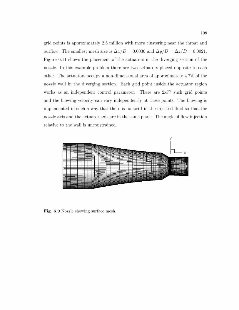
108
grid points is approximately 2.5 million with more clustering near the throat and
outflow. The smallest mesh size is ∆x/D = 0.0036 and ∆y/D = ∆z/D = 0.0021.
Figure 6.11 shows the placement of the actuators in the diverging section of the
nozzle. In this example problem there are two actuators placed opposite to each
other. The actuators occupy a non-dimensional area of approximately 4.7% of the
nozzle wall in the diverging section. Each grid point inside the actuator region
works as an independent control parameter. There are 2x77 such grid points
and the blowing velocity can vary independently at these points. The blowing is
implemented in such a way that there is no swirl in the injected fluid so that the
nozzle axis and the actuator axis are in the same plane. The angle of flow injection
relative to the wall is unconstrained.
Fig. 6.9 Nozzle showing surface mesh.

109
Fig. 6.10 Nozzle multi-block grid structure.
Fig. 6.11 The location of actuators (the blowing ports).
Fluidic inserts are known to reduce the broadband shock associated noise as well
as the mixing noise by changing the effective nozzle area ratio and introducing
streamwise vortices, as discussed by Morris et al. [30]. A method to find the

110
injection rate and distribution to achieve a desired flow behavior has been discussed
here. Figure 6.12 shows the pressure distribution inside the nozzle when there is
no blowing and the nozzle pressure ratio is fixed (NPR = 1.5). The jet is over-
expanded and a normal shock exists in the diverging section of the nozzle. The
contours represent the pressure on an azimuthal slice that passes through the
center of the two actuators. Figure 6.13 shows the pressure distribution on the
same plane when a prescribed blowing distribution has been implemented at the
actuators. The prescribed blowing distribution is given by a radial velocity,
ub = ubo exp
(−−(x− xo)2 − (y − yo)2 − (z − zo)2
2a2
)(6.83)
The blowing is implemented such that ubo is −150m/s, a is chosen to be 0.1 and
(xo, yo, zo) is the center for the blowing distribution, located at the center of the
actuator region. The positive normal at the wall is considered in the outwards di-
rection, hence the sign of the blowing speed is negative. For the two actuators, the
centers are located at a non dimensional axial distance xo/D = 0.39 downstream of
the throat, the other two coordinates are yo/D = zo/D = ±0.355. The injection of
the fluid changes the effective area ratio and even though the nozzle pressure ratio
is unchanged, there is no shock in the solution. Figure 6.14 shows the development
of counter rotating vortices caused by the blowing at the actuators. These vortices,
which are also generated in nozzles with hard-walled corrugations or fluidic inserts,
promote mixing in the jet plume, which can lead to mixing noise reductions. In the
practical situation, the blowing distribution that deflects the fluid is unknown, but
the desired pressure distribution is known to be either the ideally-expanded pres-
sure or some other prescribed pressure distribution. In the example given here, the
desired pressure distribution is considered to be the pressure distribution shown
in figure 6.13. The blowing that gives this pressure distribution is considered un-
known and the adjoint method is used to find a blowing distribution that achieves
this desired pressure distribution.

111
Fig. 6.12 The pressure distribution when there is no blowing in the divergent section.
Fig. 6.13 The pressure distribution with blowing in the divergent section.

112
Fig. 6.14 Introduction of counter rotating stream-wise vortices due to blowing.
The cost function to be minimized is given by equation (6.12), where the desired
pressure is shown in figure 6.13. The surface area in the integral is taken to be
the entire interior wall of the nozzle and supply pipe. The adjoint and direct
flow equations are solved on the same mesh as shown in figure 6.10. The spatial
terms are discretized using second order finite differences and a modified 4 stage
compact Runge-Kutta scheme is used to artificially march in time to a steady
state solution. The time step is determined by the Courant-Friedrichs-Lewy (CFL)
condition with a CFL number of 0.5. Artificial dissipation has been added to all
the equations for both calculations. The description of artificial dissipation is given
in section 3.3. The artificial dissipation coefficients in the x, y and z directions are

113
different for the direct and adjoint calculations and are chosen to be (1.3, 1.3, 1.3)
and (0.3, 0.3, 0.3) respectively. More details on the numerical method are given in
chapter 3. Figure 6.15a shows the initial difference between the desired and initial
pressures with no blowing. Figures 6.15a - 6.15d show the difference between
the current pressure distribution and the desired distribution with design cycles.
The contour scales are the same for figures 6.15a and 6.15d. The initial pressure
difference on the nozzle wall is of the order of 50,000 Pa and the final difference
goes down to the order of 5,000 Pa. The change in the cost function with design
cycle is given in table 6.2.
Table 6.2 Three-dimensional calculations: The decay of the cost function with design
cycles.
Design Cycle Normalized Cost Function Percentage decay
1 2.565x10⁻¹ 0
2 1.833x10⁻¹ 28
3 7.821x10⁻² 69
4 3.155x10⁻² 87
The decay of the cost function is almost linear with the design cycles. This is
shown in figure 6.16.

114
(a) Initial difference between desired and initial pressure on nozzle wall.
(b) Difference between desired and current pressure on nozzle wall after second
design cycle.
(c) Difference between desired and current pressure on nozzle wall after third
design cycle.
(d) Difference between desired and current pressure on nozzle wall after the fourth
design cycle.
Fig. 6.15 Variation of the pressure difference on the nozzle wall between the current
and desired pressure distribution with design cycle.

115
Fig. 6.16 The decay of cost function with design cycles.
Figures 6.17 and 6.18 show the pressure and Mach number distributions on the
nozzle centerline. The initial (grey) and desired (blue) pressure distributions are far
apart. After four design cycles, a pressure distribution close to the desired pressure
distribution is achieved using the adjoint method. Even though the desired blowing
distribution is known in the present case, it is not required by the adjoint solution
and the initial blowing velocities are set to zero. A relaxation factor of 10 has
been used for the first iteration to increase the convergence rate. After the first
iteration, this factor is no longer used in subsequent iterations. This process is
repeated until the cost function decreases to a value less than a specified tolerance.
From table 6.1 it is seen that the cost function reduces by 87% in just the first
four design cycles. The computational cost associated with each design cycle is
equal to the cost of solving the flow equations and adjoint equations once. This is
independent of the number of control parameters. There are 154 control parameters
in this example but the gradients of the cost function with respect to each of these
control parameters are calculated with no change in computational cost. This is
the major advantage of using the adjoint method.

116
Fig. 6.17 Pressure distribution on nozzle centerline with design cycles.
Fig. 6.18 Mach number distribution on nozzle centerline with design cycles.
Figure 6.19 shows the blowing that has been implemented to obtain the desired
or target pressure distribution. This blowing is applied normal to the wall in
the actuator region. Then the initial blowing normal to the wall is set to zero.
Figure 6.20 shows the blowing velocities normal to the wall after four design cycles
obtained using the adjoint method. The blowing distribution achieved by the

117
adjoint method is not same as, or even similar to, the blowing that corresponds
to the desired pressure, but the pressure distribution obtained with this blowing
is close to the desired pressure distribution as shown in figure 6.17 and by the
decrease in the cost function.
Fig. 6.19 Blowing velocity normal to the
wall used to generate the desired pressure
distribution.
Fig. 6.20 Blowing velocity normal to the
wall as given by fourth design cycle.

118
6.7 External Flow Calculations
The goal of the present research is to develop a tool to modify the shock cell
structure inside a nozzle and in the jet plume to achieve a reduction in broad-
band shock associated noise. In the previous section, it was shown that an adjoint
method can be used to recover a target pressure on the nozzle wall using surface
blowing. The present section is developed such that the external flow is included
in the calculation. It is shown that adjoint method can be used to modify the
shock cell structure using surface blowing on the nozzle wall.
The nozzle under consideration is the same as the nozzle described in section 6.6.3
and shown in figure 6.9. The external domain and shroud are added to the nozzle
using multiple additional blocks as shown in figure 6.21. The mesh is generated
using Gridgen and is shown in figure 6.22. The grid consists of 14 blocks with 5
blocks internal of the nozzle, 4 blocks in the domain external to the shroud and 5
blocks in the external domain upstream of the nozzle exit, constituting a total of
5.7 x 10⁶ points. Figure 6.23 shows the placement of the actuators on the nozzle
wall. Three actuators are placed in the diverging section of the nozzle domain with
25 grid points in each actuator. The actuators are placed symmetrically on the
nozzle diverging section.
The spatial terms are discretized using second order finite differences and a modi-
fied 4 stage compact Runge-Kutta scheme is used to artificially march in time to a
steady state solution. The time step is determined by the Courant-Friedrichs-Lewy
(CFL) condition with a CFL number of 0.5. Artificial dissipation has been added
to all the equations for both calculations. The artificial dissipation coefficients in
the x, y and z directions are different for the direct and adjoint calculations and
are chosen to be (1.3, 1.3, 1.3) and (0.3, 0.3, 0.3) respectively. More details on the
numerical method are given in chapter 3.

119
Fig. 6.21 The placement of blocks when the external domain is included.

120
Fig. 6.22 The mesh including the external domain.
Fig. 6.23 The location of symmetrically placed actuators in the nozzle diverging section.
The approach based on the adjoint method is same as the previous section. The
details of the approach are omitted to avoid repetition. The exit to throat area

121
ratio of the nozzle is 1.176. The nozzle pressure ratio for ideal expansion and
the design Mach number for the nozzle under consideration are 3.6768 and 1.5
respectively. The operating conditions are such that the pressure ratio is 4.58
so the nozzle is under-expanded for this pressure ratio and there are expansion
waves in the nozzle jet plume. The Mach number contours are shown in figure
6.24. An adjoint method is incorporated to get the flow field close to the desired
flow as shown in figure 6.25. Three design cycles are run where the normalized
cost function drops from a value of 66.07 to 3.58. The cost function is normalized
with respect to the total pressure and unit length. The Mach number contours
corresponding to design cycles 1, 2 and 3 are shown in figures 6.26, 6.27 and 6.28
respectively. A comparison of the final (figure 6.28) and desired solution (figure
6.25) shows that the two solution are close to each other. This is also reflected by
the small value of cost function (3.5).
Fig. 6.24 The Mach number contours for the nozzle operating with 4.58 nozzle pressure
ratio and no blowing.

122
Fig. 6.25 The Mach number contours for the nozzle operating with 4.58 nozzle pressure
ratio and the desired blowing.
Fig. 6.26 The Mach number contours after the first design cycle for the nozzle operating
with 4.58 nozzle pressure ratio.

123
Fig. 6.27 The Mach number contours after the second design cycle for the nozzle oper-
ating with 4.58 nozzle pressure ratio.
Fig. 6.28 The Mach number contours after third design cycle for the nozzle operating
with 4.58 nozzle pressure ratio.

124
6.8 Conclusion
Two and three-dimensional calculations have been performed to achieve a desired
pressure distribution on the nozzle wall. The adjoint design method has been im-
plemented to determine the blowing distribution on a fixed region of the nozzle
wall known as the actuator. The blowing distributions as described have no con-
straints applied, except that the injection locations are fixed. This can be modified
by adding additional constraints on the blowing distribution. These constraints
could be applied to make sure that the blowing starts smoothly at the ends of
the actuator region. In addition the blowing velocity and its derivative could be
required to be zero at the end locations. These constraints can be incorporated
into the definition of the Lagrange functional. In both two and three-dimensional
cases, the adjoint method takes 3 - 4 design cycles to achieve a reduction of the
order of 60% to 80% in the cost function. When the desired pressure is calculated
using a known blowing distribution, the adjoint method is found to find a different
blowing distribution that gives a pressure distribution close to desired pressure dis-
tribution. This implies that there is more than one local minimum in the solution
space and the adjoint method finds one of these minima.
6.9 Summary
In this chapter, an adjoint approach to determine the required blowing on a nozzle
wall has been described. The blowing velocity components are considered to be
independent design parameters and the optimum value of the control parameters
is found using an adjoint approach. The advantage of using the adjoint approach
is that the computational cost of calculating the sensitivities of the cost function
to change in the control parameters is almost independent of the number of design
parameters. The adjoint approach is very effective in cases where there are sev-
eral design parameters to be considered. Several examples of the optimization of
125
blowing are given in this chapter. In the first example the desired pressure distri-
bution was calculated for a giving blowing distribution. In the second, the blowing
distribution required to achieve ideal expansion in the nozzle was obtained. First,
two-dimensional calculations were performed and the approach was then extended
to three-dimensional calculations. It has been shown that an adjoint design method
takes less than 10 design cycles to reach a pressure distribution close to the desired
pressure distribution in the cases considered.
Conclusions from the described approaches and results are given in the next chap-
ter. There are several ideas for future development and a lot of scope to the use of
adjoint equations. The adjoint approach can be used to optimize other quantities
such as vorticity generation. The adjoint approach can be used to optimize the
shape of the fluidic injectors or the nozzle exit seals. These ideas are discussed in
the final chapter.

126
Chapter 7Conclusions and Future Work
The use of adjoint methods for aerodynamic optimization has been increasing. The
two primary reasons for the use of adjoint methods are the flexibility they offer
in terms of choosing a cost function or control parameters and the computational
cost taken by adjoint methods is almost independent of the number of design pa-
rameters. Several design parameters can be considered without a great increase in
the computational cost that it takes to compute the sensitivities of a cost function
with respect to these design parameters. Motivated by the development of “fluidic
inserts,” an adjoint method to optimize the rate of injection such that a desired
pressure distribution is achieved inside the nozzle has been developed. Fluidic
inserts are devices that are used to inject by-pass air into the nozzle core flow to
achieve jet noise reduction. Two approaches to consider the blowing velocity on
the nozzle wall as the control parameters have been given.
Jet noise is generated due to the turbulent mixing of the jet shear layer with the
atmosphere (mixing noise) and due to the existence of shock cells in the jet plume
(broadband shock associated noise). The shock cell structure in the jet plume
exists when the nozzle is operating such that the exit pressure does not match
the ambient pressure. The pressure then adjusts to the ambient pressure through
shocks and expansions. It has been shown that the incorporation of flow injection
on the nozzle walls can help in achieving a reduction in both noise components [28].

127
The injection of the fluid works in two ways to reduce both noise components: the
broadband shock associated noise and the mixing noise. The injection of fluid on
the wall moves the flow away from the wall, actively “morphing” the nozzle inner
contour while keeping the geometry of the nozzle fixed. This active morphing of
the inner contour changes the effective exit to throat area ratio of the nozzle which
can help in achieving a flow field similar to the ideally expanded condition, even
when the nozzle is operating at off-design conditions. The injection of fluid also
introduces stream-wise vortices into the jet plume. These vortices help to increase
the turbulent mixing and result in a decrease in the mixing noise. Finding the
optimum rate of injection is a challenge. In this thesis an adjoint method has been
used to optimize the nozzle wall blowing as a first step in the optimization of the
fluid inserts.
Two adjoint approaches have been developed. The first approach is such that the
blowing velocity is written as a combination of a set of basis functions multiplied
by the appropriate coefficients. These coefficients of the basis functions are consid-
ered as the control parameters. An adjoint method is then developed to find the
optimum value of these design parameters. The nozzle geometry and operating
conditions are kept fixed. The location of the actuators (blowing ports) is also
kept fixed. Two examples of optimization are given. The first example considers
a Gaussian blowing distribution dependent on only one design parameter. The
desired or target pressure is found using a known blowing distribution. The ad-
joint method is then used to find the value of the design parameter: that is, the
amplitude of the blowing distribution. The amplitude of the blowing is recovered
within 1.6% error in 3 design cycles. The second example is set up to obtain a
nearly uniform pressure distribution in the nozzle divergent section. In this case
the blowing velocity depends on three design parameters. The optimum value of
these parameters is found using the adjoint method.

128
A second adjoint approach for the optimization of blowing has been developed to
offer more flexibility. The approach allows for the use of any kind of design/control
parameters. For practical purposes, the design parameters are chosen as the blow-
ing velocities at a number of fixed nozzle wall points. Two and three-dimensional
calculations are performed and it is demonstrated that with the use of the adjoint
method the optimum blowing distribution can be found in 4-5 design cycles. The
optimum blowing distribution is the blowing distribution that gives a pressure dis-
tribution close to the target distribution. This target pressure distribution can be
found in two ways. It can be found using a known blowing distribution, or for
more practical case, it can correspond to nearly ideally expanded flow. The blow-
ing to achieve a pressure distribution close to the target pressure is found using
the adjoint method. It is shown that with the use of the adjoint method, a blowing
distribution on the nozzle wall can be found such that the pressure distribution is
close to that for ideal expansion irrespective of the nozzle operating conditions.
A multi-block structured mesh is used for the three-dimensional calculations. Multi-
block grids are generated for relatively complex geometries. However, this can
result in grid singularities. The whole domain is divided into multiple Cartesian
blocks. The block interfaces are considered as separate boundaries. The required
block interface conditions for the direct and adjoint problems have been derived.
These boundary conditions are based on the method of characteristics. The resid-
uals (or time derivatives) in a block are either replaced or retained based on the
direction of propagation of information. This direction is determined by the char-
acteristics of the flow or adjoint equations. It is shown that adjoint characteristics
travel in the opposite direction to the direct flow characteristics.

129
Recommendations for Future Work
The scope for the future usage of adjoint methods in the field of noise reduction is
very wide. The development of the method presented in this thesis is generic and
can be modified to incorporate several changes and additions. The calculations
performed here are presented for the inviscid Euler equations. The same approach
can be used to add viscous effects and a turbulence model. An important next step
would be to perform unsteady calculations to be able to perform noise predictions.
The introduction of blowing on the nozzle wall introduces counter rotating vortices
in the flow field. These vortices help in reducing the mixing noise by increasing
the turbulent mixing. The strength of these vortices can be optimized using the
adjoint approach. A measure of the magnitude of the stream-wise vorticity can be
added to the cost function while continuing to require a targeted pressure distri-
bution.
The blowing distributions as described here have no constraints applied, except
that the injector locations are fixed. This can be modified by adding additional
constraints on the blowing distribution. These constraints could be applied to
make sure that the blowing starts smoothly at the edges of the actuator region.
For example, the blowing velocity and its derivative could be required to be zero
at the edge locations. These constraints can be incorporated into the definition of
the Lagrange functional. The approach described in this thesis can be extended to
implement these changes. However, the locations of the injectors can be limited
to the experimental locations such as in the experiments of Morris et al. [28].
Due to the presence of a shock there is a discontinuity in the cost function. In this
case the cost function can be redefined such that it is smooth even at the location
of the shock. Also, a term quantifying the pressure gradient can be added to the
cost function to reduce the shock and expansion strengths with the aim of reducing
130
the broadband shock associated noise.
The use of adjoint methods for shape optimization has been the subject of much
prior research. In the context of the present application, the adjoint method could
be used to optimize the shape of the injectors. The shape of the injectors can be
parameterized and an adjoint approach can be used to obtain an optimum shape
to achieve the greatest noise reduction with the use of fluidic inserts.
The cost functions described in the thesis have involved properties integrated over
a sensor surface or surfaces. Volume integrals can also be considered. For example,
the cost function could involve an integral of the pressure variations, or some other
parameter such as the turbulent kinetic energy, in the entire jet plume. In this
case the adjoint equations will contain source terms and these will drive the adjoint
solution, as opposed to the boundary condition forcing described in this thesis.

131
Appendix AThe Solver Development
A solver to find the numerical solution to the direct and adjoint equations and
for the calculation of sensitivities has been developed for the research presented in
this thesis. An optimizing technique has been implemented in the solver to find
the new set of design parameters. The details on the structure of the code, input
and output file formats and other details of the solver development are given in
this chapter.
A.1 Code Structure
All subroutines have been written in the FORTRAN90 language and the solver is
portable to the linux clusters. Figures A.1 and A.2 show the basic structure of the
code. The first step of the process is to calculate the desired flow conditions. The
direct solver is first called to solve for the desired flow based on the specific method
to calculate the desired flow as explained in chapters 5 and 6. This output is stored
in a file and then it is read by the direct-adjoint design solver. The direct-adjoint
design solver starts by calling the direct solver first to calculate a steady state
solution of the direct equations for a given set of design parameters. This solution
is then used by the adjoint solver that solves for the adjoint equations. Both adjoint
and direct solutions are then fed into the sensitivity calculation subroutine. The
sensitivity calculation subroutine first calculates the cost function and then finds
the sensitivities of the cost function with respect to the design parameters. These

132
sensitivities are used in an optimizing technique to calculate the design parameters
for the next design cycle.

133
Initialize
Allocate stack memory
Read input Grid and boundary condition files
Input parameters
Allocate heap (dynamic) memory
Read desired flow conditions Initialize flow variables
and fluxes
Direct flow solver
Start time loop
End time loop
Calculate flow fluxes
Calculate time derivatives Add dissipation
Flow variables at the next time step
Residual correction boundary condition
Boundary conditions on flow variables
Stages of time marching scheme
Overwrite new flow values in the old ones
Repeat based on the time marching scheme
Write intermediate restart files
Exit if convergence is achieved
Calculate time step
Print solution files
Fig. A.1 The code structure to find direct and adjoint solutions and optimization of the
cost function - continued to next figure

134
Adjoint flow solver
Initialize adjoint variables
Start time loop
End time loop
Calculate adjoint vectors
Calculate time derivatives Add dissipation
Adjoint variables at the next time step
Residual correction boundary condition
Boundary conditions on flow variables
Stages of time marching scheme
Overwrite new adjoint values in the old ones
Repeat based on the time marching scheme
Write intermediate restart files
Exit if convergence is achieved
Print solution files
Optimizer
Calculate sensitivities
Calculate new values of design parameters
Go to direct flow solution
Fig. A.2 The code structure to find direct and adjoint solutions and optimization of the
cost function

135
A.2 Input requirements
Input parameters
The following inputs are given to the solver,
1. Flow parameters
2. Grid file
3. Boundary condition file
Table A.1 Input Parameters: the values of fluid properties, convergence criteria, inlet
and ambient conditions, initial conditions and numerical parameters.
variable parameter
NPR Pressure ratio
P0 total pressure
pa ambient pressure
T0 total temperature
gama ratio of specific heats
mu coefficient of viscosity
gasconst gas constant
CFL Courant number
Cx, Cy, Cz Coefficients of dissipation
ki tmp intermediate solution printing frequency
tn Initial condition indicator
if 0; uniform initialization
if 1; gaussian pulse initialization
if 2; initial condition read from a file

136
Input files
There are four input files that are required by the solver. The boundary condition
file and grid file generated by gridgen are the input files for the solver. The other
two files are the gas properties file and the input parameters file.
Boundary conditions file
The boundary condition files are generated by gridgen when the solver is set to
generic. The boundary conditions are indicated by the regions of blocks and the
initial and final indices in all three directions. The index that defines the region
has the same value for initial and final index. The boundary condition is specified
by a number. The specific boundary conditions are noted in the table A.2.
Table A.2 Boundary Conditions: the number that specify the type of boundary condition
at a given boundary
Indicator Boundary Condition
2 Slip wall
3 Symmetry
5 Inflow
6 Outflow
8 Two dimensional
9 Atmospheric inflow
11 Radiation bc
51 Reimann variant
-1 Interface
The grid file is read in the PLOT3D file format. The grid metrics are calculated
inside the code using the values of (x, y, z) coordinates and a second order finite

137
difference scheme. A Fortran code fragment for a Gridgen style volume grid file
follows:
c.....number of grid points in block integer ni(nmax), nj(nmax), nk(nmax)
c.....grid point coordinates
real x(imax,jmax,kmax), y(imax,jmax,kmax), z(imax,jmax,kmax)
write(1) nblocks
do mb = 1, nblocks
write(1) ni(mb), nj(mb), nk(mb)
write(1) (((x(i,j,k),i=1,ni(mb)),j=1,nj(mb)),k=1,nk(mb)),
(((y(i,j,k),i=1,ni(mb)),j=1,nj(mb)),k=1,nk(mb)),
(((z(i,j,k),i=1,ni(mb)),j=1,nj(mb)),k=1,nk(mb))
end do
The boundary condition file is in the following format,
write flow solver id
write number of blocks

138
do number of blocks
write block imax, block jmax,
(and block kmax if 3D), block name
c........a region is a boundary condition or interblock connection write num-
ber of regions on block
c........a region is a boundary condition or interblock connection write number of regions on block
c..............For an interblock connection, there are three
c..............pairs of indices that must be matched (three on
c..............the source face and three on the target face).
c..............The index that’s constant on both the source and
c..............target faces is easy to determine simply by
c..............comparing the min and max indices and finding the
c..............pair in which min and max are the same.
c..............On each of the source and target faces, Gridgen
c..............writes one of the two remaining min-max index
c..............combinations as negative numbers. The negative
c..............min-max pair on each face correspond. Once you
c..............determine the corresponding negative indices
c..............just convert them to positive numbers.
c..............That leaves one pair of indices that align.
c..............Keep in mind that the max index may actually
c..............be less than the min index. You can either use
c..............a negative increment to step through the index
c..............or you can swap the min and max indices on BOTH
c..............source and the matching target indices.

139
write target region imin, target region imax, target region jmin, target region jmax,
(and target region kmin, target region kmax if target block number
endif
end do number of regions on block
end do number of blocks
A.3 Output files
The output files are solution files at a specified time interval. The output files can
be written in two file formats, namely, tecplot file format and plot3D file format.
140
Appendix BGoverning and Adjoint Equations inCurvilinear Coordinates
This sections lists the governing equations and adjoint used to solve the flow-field.
The Euler equations and adjoint equations as developed in chapter 6 are written
in curvilinear coordinates to solve the equations on a multi-block structured grid.
The grid is transformed using a grid transformation matrix from the physical do-
main (x, y, z) to the computational domain (ξ, η, ζ) and the governing equations
are re-written to comply with the computational domain coordinates.
The governing equations are presented here in three dimensions. The equations
for two dimensional or one dimensional calculations can be derived by setting the
derivatives in the ζ, or η and ζ directions to zero respectively. The generalized
coordinates (ξ, η, ζ) are a function of physical coordinates (x, y, z) and can be
written as equation B.1:
ξ = ξ(x, y, z)
η = η(x, y, z)
ζ = ζ(x, y, z)
(B.1)

141
and the Jacobian transformation matrix used to relate the computational and
physical coordinates is defined as given in equation B.2:
J =
∣∣∣∣∂(ξ, η, ζ)
∂(x, y, z)
∣∣∣∣ =
∣∣∣∣∣∣∣∣∣ξx ξy ξz
ηx ηy ηz
ζx ζy ζz
∣∣∣∣∣∣∣∣∣ =
∣∣∣∣∣∣∣∣∣xξ xη xζ
yξ yη yζ
zξ zη zζ
∣∣∣∣∣∣∣∣∣−1
(B.2)
where ∂ denotes the partial derivative, det denotes the determinant and subscripts
represent partial derivatives. The unit normal vector at a grid point along a
constant ξ value, denoted by ~lξ, is defined as:
~lξ =
ξx|5ξ| ,
ξy|5ξ| ,
ξz|5ξ|
(B.3)
where, | 5 ξ| =√ξ2x
+ ξ2y
+ ξ2z. Similar forms can be used to derive unit normal
vectors in the η and ζ directions. These values are typically used in boundary
condition implementation: for example, to calculate the flow direction (inflow or
outflow) on a computational face. The transformation from physical to computa-
tional domain is applied to the dimensional direct and adjoint Euler equations and
the transformed equations are obtained as shown in equation B.4:
∂Q
∂t+∂E
∂ξ+∂F
∂η+∂G
∂ζ= 0 (B.4)
Variables with hat, for example Q, are in generalized curvilinear coordinates. They
are a function of flow variables in Cartesian coordinates and are related to them
as shown in equations B.5 - B.8:
Q =Q
J=
1
J
ρ
ρu
ρv
ρw
ρe
(B.5)

142
E =ξxE + ξyF + ξzG
J=
1
J
ρU
ρUu+ ξxp
ρUv + ξxp
ρUw + ξxp
(ρe+ p)U
(B.6)
F =ηxE + ηyF + ηzG
J=
1
J
ρV
ρV u+ ηxp
ρV v + ηxp
ρV w + ηxp
(ρe+ p)V
(B.7)
G =ζxE + ζyF + ζzG
J=
1
J
ρW
ρWu+ ζxp
ρWv + ζxp
ρWw + ζxp
(ρe+ p)W
(B.8)
In the equations B.6 - B.8, U , V and W are the contravariant velocities in the
three generalized coordinate directions. The variables ρ, p and e are the density,
pressure and total energy respectively. u, v and w are the velocity components in
the three directions. The contravariant velocities can be calculated as:
U = ξxu+ ξyv + ξzw (B.9)
V = ηxu+ ηyv + ηzw (B.10)
W = ζxu+ ζyv + ζzw (B.11)

143
The derivatives such as ∂/∂x can be calculated from the generalized coordinates
as,
∂
∂x= ξx
∂
∂ξ+ ηx
∂
∂ξ+ ζx
∂
∂ξ(B.12)
∂
∂y= ξy
∂
∂ξ+ ηy
∂
∂ξ+ ζy
∂
∂ξ(B.13)
∂
∂z= ξz
∂
∂ξ+ ηz
∂
∂ξ+ ζz
∂
∂ξ(B.14)
The partial derivatives can be calculated by using spatial discretization schemes
such as MacCormach scheme. The grid transformation matrices are calculated
using the second order central differencing schemes. Since the form of adjoint
equations are exactly the same as the direct equation as given by (B.4), exactly
the same approach is used to transform the adjoint equations from physical space
to the computational domain.
144
Bibliography
[1] M. B. Alkislar, A. Krothapalli, and G. W. Butler. The effect of streamwise vorticeson the aeroacoustics of a Mach 0.9 jet. Journal of Fluid Mechanics, 578:139–169,2007.
[2] T. R. Bewley, P. Moin, and R. Temam. DNS-based predictive control of turbu-lence: an optimal benchmark for feedback algorithms. Journal of Fluid Mechanics,447:179–225, 2001.
[3] K. S. Brentner and F. Farassat. Analytical comparison of the acoustics analogy andkirchhoff formulation for moving surfaces. AIAA Journal, 36(8:1379–1386, 1998.
[4] J. Bridges and C. A. Brown. Parametric testing of chevrons on single flow hot jets,2004. AIAA Paper 2004-2824.
[5] J. Bridges and C. A. Brown. Parametric testing of chevrons on single flow hotnozzles, 2004. AIAA Paper No. 2004-2824.
[6] S. S. Collis, K. Ghayour, and M. Heinkenschloss. Optimal transpiration boundarycontrol for aeroacoustics. AIAA Journal, 41:1257–1270, 2003.
[7] A. W. Correia, J. L. Peters, J. I. Levy, S. Melly, and F. Dominici. Residentialexposure to aircraft noise and hospital admissions for cardiovascular diseases: multi-airport retrospective study. British Medical Journal, 3:347:f5561, 201.
[8] M. J. Doty and D. K. McLaughlin. Acoustic and mean flow measurements of high-speed, helium-air mixture jets. International Journal of Aeroacousticsl, 50:293–334,2003.
[9] Y. Du. Supersonic jet noise prediction and noise source investigation for realisticbaseline and chevron nozzles based on hybrid RANS/LES simulations. PhD thesis,Pennsylvania State University, 2011.
[10] J. Freund. Adjoint-based optimization for understanding and suppressing jet noise.Procedia Engineering, 6:54–63, 2010.
[11] M. B. Giles and N. A. Pierce. An introduction to the adjoint approach to design.Flow, Turbulence and Combustion, 65(3-4):393–415, 2000.

145
[12] M. Hayashi, M. Ceze, and E. Volpe. Characteristics-based boundary conditions forthe euler adjoint problem: 2-d formulation. In 28th AIAA Applied AerodynamicsConference, Chicago, Illinois, 2010. AIAA Paper No. 2010-4677.
[13] B. Henderson and J. Bridges. An MDOE investigation of chevrons for supersonicjet noise reduction, 2010. AIAA Paper No. 2010-3926.
[14] A. Jameson. On optimum design in fluid mechanics. Journal of Scientific Comput-ing, 3:233–260, 1988.
[15] A. Jameson. Optimum aerodynamic design using CFD and control theory, 1995.AIAA Paper 95-1729.
[16] R. D. Joslin, M. D. Gunzburger, and R. A. Nicolaides. Self-contained automatedmethodology for optimal flow control. AIAA Journal, 35(5):816–824, 1997.
[17] B.-J. Jung, H. M. Kim, X. Z. T. Aulign, X. Zhang, , and X.-Y. Huang. Adjoint-derived observation impact using wrf in the western north pacific. American Mete-orological Society Journal, 141:4080–4097, November 2013.
[18] J. Kim, D. J. Bodony, and J. B. Freund. Aeroacoustics control of a turbulent mach1.3 jet using adjoint-based optimization, 2011. AIAA Paper 2011-2832.
[19] J.-H. Kim, Kearney-Fischer, M. M., Samimy, and S. Gogineni. Far-field noise controlin supersonic jets using conical and contoured nozzles. ASME Journal of Engineer-ing for Gas Turbine and Power, 133:081201–1 to 081201–9, August 2011.
[20] J. W. Kim and D. J. Lee. Characteristic interface conditions for multiblock high-order computation on singular structured grid. AIAA Journal, 41:2341–2348, 2003.
[21] K. Kinzie, B. Henderson, J. Whitmire, and A. Abeysinghe. Fluidic chevrons forjet noise reduction, 2004. ACTIVE 04: 2004 International Symposium on ActiveControl of Sound and Vibration; 20-22 Sep.; Williamsburg, VA; United States.
[22] A. Kohl and Willerband. An adjoint method for the assimilation of statisticalcharacteristics into eddy-resolving ocean models, 2002. Tellus A, 54: 406-425. doi:10.1034/j.1600-0870.2002.01294.x.
[23] A. Krothapalli, L. Ventkatakrishnan, L. Lourenco, B. Greska, and R. Elavarasan.Turbulence and noise suppression of a high-speed jet by water injection. Journal ofFluid Mechanics, 491:131–159, 2003.
[24] C.-W. Kuo, P. J. Morris, and M. D. K. Noise reduction in supersonic jets by fluidicnozzle inserts, 2012. AIAA Paper 2012-2210.
[25] B. J. Lee and M.-S. Liou. Unsteady adjoint approach for design optimization offlapping airfoils. AIAA Journal, 50:2460–2475, 2012.
[26] J. L. Lions. Optimal Control of Systems Governed by Partial Differential Equations.Springer-Verlag, Berlin, 1971.

146
[27] D. K. McLaughlin, J. Bridges, and C.-W. Kuo. On the scaling of small, heat sim-ulated jet noise measurements to moderate size exhaust jets. International Journalof Aeroacoustics, 9:627–654, 2010.
[28] P. J. Morris and D. K. McLaughlin. Methods and apparatus for providing fluidicinserts into an exhaust stream to reduce jet noise from a nozzle. USA ProvisionalPatent Application 61/648,441, May 2012.
[29] P. J. Morris and D. K. McLaughlin. High speed jet noise reduction: past progressand future possibilities, 2013. AIAA Paper No. 2013-0006.
[30] P. J. Morris, D. K. McLaughlin, and C.-W. Kuo. Noise reduction in supersonic jetsby nozzle fluidic inserts. Journal of Sound and Vibration, 332:3992–4003, 2013.
[31] P. J. Morris, N. Sikarwar, D. K. McLaughlin, C. W. Kuo, and M. Lurie. Adjointdesign methods for nozzles for reduced noise in high-speed jets, 2012. AIAA PaperNo. 2012-3821.
[32] D. Munday, N. Heeb, E. G. Markus, O. Burak, and L.-E. Eriksson. Supersonicjet noise from a conical c-d nozzle with forward flight effects. AIAA Journal,50(11):2336–2350, Nov 2012.
[33] S. Nadarajah and A. Jameson. A comparison of the continuous and discrete adjointapproach to automatic aerodynamic optimization, 2000. AIAA 38th AerospaceSciences Meeting and Exhibit, AIAA-2000-0667.
[34] C. Nelson. An overview of the nparc alliance’s wind-us solver, 2010. AIAA Paper2010-0027l.
[35] M. Nemec, M. J. Aftosmis, and M. Wintzer. Adjoint-based adaptive mesh refine-ment for complex geometries, 2008. 46th AIAA Aerospace Sciences Meeting.
[36] B. P. Petitjean, D. K. McLaughlin, and K. Viswanathan. Acoustic pressure wave-forms measured in high speed jet noise experiencing nonlinear propagation. Inter-national Journal of Aeroacoustics, 5:193–215, 2006.
[37] O. Pironneau. On optimum design in fluid mechanics. Journal of Fluid Mechanics,64:97–110, 1974.
[38] R. W. Powers, D. K. McLaughlin, P. J. Morris, and C. W. Kuo. Supersonic jetnoise reduction by nozzle fluidic inserts with simulated forward flight. In 20thAIAA/CEAS Aeroacoustics Conference, Atlanta, GA, 16 - 20 June 2014.
[39] M. Samimy, J.-H. Kim, J. Kastner, I. Adamovich, and Y. Utkin. Active control ofhigh speed and high reynolds number jets using plasma actuators. Journal of FluidMechanics, 578:305–330, May 2007.
[40] J. M. Seiner. Advances in high speed jet aeroacoustics, 1984. AIAA Paper 84-2275.
[41] J. M. Seiner. Method and device for reducing engine noise, January 2009. USAPatent US 7,475,550 B2.

147
[42] J. M. Seiner, L. S. Ukeiley, and B. Jansen. Aero-performance efficient noise reductionfor the F404-400 engine, 2005. AIAA Paper No. 2005-3048.
[43] N. Sikarwar. The use of adjoint methods in jet nozzle design, 2009. Masters Thesis,Pennsylvania State University.
[44] N. Sikarwar and P. J. Morris. Optimization of blowing in a convergent-divergentnozzle for noise reduction. In 20th AIAA/CEAS Aeroacoustics Conference, 16 - 20June 2014. AIAA Paper No. 2014-2473.
[45] N. Sikarwar and P. J. Morris. The use of adjoint method for optimization of blowingin a convergenct-divergent nozzle. International Journal of Aeroacoustics, 14:327–351, 2015.
[46] D. A. Venditti and D. L. Darmofal. Adjoint-derived observation impact using wrfin the western north pacific. Journal of Computational Physics, 164:204–227, 2000.
[47] K. Viswanathan, M. Shur, M. Strelets, and P. R. Spalart. Numerical prediction ofnoise from round and beveled nozzles, July 18-20, 2005. Euromech Colloquium 467:Turbulent Flow and Noise Generation.
[48] Q. Wang, P. Moin, and G. Iaccarino. Minimal repetition dynamic checkpointingalgorithm for unsteady adjoint calculation. SIAM Journal on Scientific Computing,31:25492567, 2009.
[49] M. Wei and J. B. Freund. A noise-controlled free shear layer. Journal of FluidMechanics, 546:123–152, 2006.

NIDHI [email protected]
412-638-9887
Education
• Pennsylvania State UniversityPh.D. in Aerospace Engineering, defended December 2014 GPA: 3.93/4.0
– Ph.D. minor in Computational Science GPA: 4.0/4.0
• Pennsylvania State UniversityM. S. in Aerospace Engineering, graduated December 2009 GPA: 3.96/4.0
• Indian Institute of Technology, Kanpur, IndiaB. Tech. in Aerospace Engineering, graduated June 2007 GPA: 8.40/10
Work Experience
• The Use of Adjoint Method in Optimization of Blowing in a C-D Nozzle to Achieve Noise ReductionPennsylvania State University, Graduate Research Assistant, Advisor: Dr. Philip Morris
– Developed and implemented adjoint method for optimization of active flow control.
– Developed a multi-block, three-dimensional, parallel RANS solver for the nozzle flows.
– Developed a multi-block, three-dimensional, parallel adjoint solver.
– Developed and implemented a method of characteristics block interface boundary conditions for adjointequations.
– Generated various 3D multi-block grids using CAD designs and gridgen to run the above solvers.
• LES Simulation of Supersonic Jet FlowPennsylvania State University, Graduate Research Assistant, Advisor: Dr. Philip Morris
– Gained experience in working with large, multi-modular, parallel code.
– Provided support to Pratt & Whitney for setting up, running and troubleshooting the code.
• Development of Adjoint Method to Design the Nozzle Contour in Order to Optimize the NoisePennsylvania State University, Graduate Research Assistant, Advisor: Dr. Philip Morris
– Developed and implemented Adjoint method for automatic optimization of the nozzle geometry of a jetaircraft.
Publications
• Nidhi Sikarwar, Philip Morris: “The Use of an Adjoint Method for Optimization of Blowing in aConvergent-Divergent Nozzle”, International Journal of Aeroacoustics, vol 14, number 1 & 2, pp 327 - 351,2015.
• Nidhi Sikarwar, Philip Morris: “Characteristics Boundary Conditions to Treat Adjoint Block Interfaces”,IEEE Aerospace Conference 2015, MAR 7 - 15, 2015, Big Sky, MT.
• Nidhi Sikarwar, Philip Morris: “Optimization of Blowing in a Convergent-Divergent Nozzle for NoiseReduction”, AIAA Paper No. 2014,-2473, 2014.
• Philip Morris, Nidhi Sikarwar, D. K. McLaughlin, C. W. Kuo and M. Lurie: “Use of AdjointDesign Methods for Nozzles for Reduced Noise in High-speed Jets”, AIAA Paper No. 2012-3821, 2012.
• Nidhi Sikarwar, Satya Prakash, Biju Uthup: “Understanding Viscous Flow Field on a Cropped DoubleDelta Wing at High Angles of Attack”, 9th annual CFD symposium, The Aeronautical Society of India andNational Aeronautical Laboratories, Bangalore, August 2006.
• Nidhi Sikarwar, Ashutosh Chauhan: “Use of Machine Learning to Optimize Fluidic Inserts”, acceptedby : AVIAION 2015.