the control and stability analysis of two–wheeled road vehicles
181
T HE C ONTROL AND S TABILITY A NALYSIS OF T WO – WHEELED ROAD V EHICLES S IMOS E VANGELOU Submitted to the University of London for the degree of Doctor of Philosophy Electrical and Electronic Engineering Imperial College London September 2003
Transcript of the control and stability analysis of two–wheeled road vehicles
THE CONTROL AND STABILITY ANALYSIS
OF TWO–WHEELED ROAD VEHICLES
SIMOS EVANGELOU
Submitted to the University of London
for the degree of
Doctor of Philosophy
Electrical and Electronic Engineering
Imperial College London
September 2003
Abstract
The multibody dynamics analysis software, AUTOSIM, is used to develop automated linear and
nonlinear models for the hand derived motorcycle models presented in (Sharp, 1971, 1994b). A
more comprehensive model, based on previous work (Sharp and Limebeer, 2001), is also derived
and extended. One version of the code uses AUTOSIM to produce a FORTRAN or C program
which solves the nonlinear equations of motion and generates time histories, and a second ver-
sion generates linearised equations of motion as a MATLAB file that contains the state-space
model in symbolic form. Local stability is investigated via the eigenvalues of the linearised
models that are associated with equilibrium points of the nonlinear systems. The time histories
produced by nonlinear simulation runs are also used with an animator to visualise the result. A
comprehensive study of the effects of acceleration and braking on motorcycle stability with the
use of the advanced motorcycle model is presented. The results show that the wobble mode of
a motorcycle is significantly destabilised when the machine is descending an incline, or brak-
ing on a level surface. Conversely, the damping of the wobble mode is substantially increased
when the machine is ascending an incline at constant speed, or accelerating on a level surface.
Except at very low speeds, inclines, acceleration and deceleration appear to have little effect on
the damping or frequency of the weave mode. A theoretical study of the effects of regular road
undulations on the dynamics of a cornering motorcycle with the use of the same model is also
presented. Frequency response plots are used to study the propagation of road forcing signals to
the motorcycle steering system. It is shown that at various critical cornering conditions, regular
road undulations of a particular wavelength can cause severe steering oscillations. The results
and theory presented here are believed to explain many of the stability related road accidents
that have been reported in the popular literature. The advanced motorcycle model is improved
further to include a more realistic tyre-road contact geometry, a more comprehensive tyre model
based on Magic Formula methods utilising modern tyre data, better tyre relaxation properties
and other features of contemporary motorcycle designs. Parameters describing a modern high
performance machine and rider are also included.
1
Acknowledgements
I wish to thank Professor David Limebeer and Professor Robin Sharp for their support and
guidance throughout this project and for taking care of the necessary funding. It has been a
unique experience to work with such outstanding researchers and to know that I could constantly
trust their scientific judgements, which, I must say, they always explained with great enthusiasm.
I really enjoyed their pleasant, humorous and open-hearted character and I doubt I will ever
forget the exhilarating trip to Snetterton race track on the back seat of Prof. Limebeer’s Kawasaki
ZX-9R.
Finally, my deepest gratitude goes towards my family for their endless love and support.
Their confidence in me has been tremendously encouraging and provided me with strength to
accomplish my task. I feel very lucky to have such a caring family and to know that I can always
rely upon them.
2
Contents
Abstract 1
Acknowledgements 2
List of Figures 7
List of Tables 13
I Introduction and Literature Review 14
1 Introduction 15
2 Literature Review 18
II Motorcycle Models 34
3 The Sharp 1971 motorcycle model 36
3.1 Physical description of the model . . . . . . . . . . . . . . . . . . . . . . . . . 36
3.2 Programming of the model . . . . . . . . . . . . . . . . . . . . . . . . . . . . 37
3.2.1 Body structure diagram . . . . . . . . . . . . . . . . . . . . . . . . . . 37
3.2.2 Program code . . . . . . . . . . . . . . . . . . . . . . . . . . . . . . . 37
3.3 Simulations and Results . . . . . . . . . . . . . . . . . . . . . . . . . . . . . . 46
3.4 Conclusions . . . . . . . . . . . . . . . . . . . . . . . . . . . . . . . . . . . . 47
4 The Sharp 1994 motorcycle model 48
4.1 Physical description of the model . . . . . . . . . . . . . . . . . . . . . . . . . 48
4.2 Programming of the model . . . . . . . . . . . . . . . . . . . . . . . . . . . . 49
4.2.1 Body structure diagram . . . . . . . . . . . . . . . . . . . . . . . . . . 49
4.2.2 Program codes . . . . . . . . . . . . . . . . . . . . . . . . . . . . . . 51
4.3 Simulations and Results . . . . . . . . . . . . . . . . . . . . . . . . . . . . . . 66
4.4 Conclusions . . . . . . . . . . . . . . . . . . . . . . . . . . . . . . . . . . . . 67
3
5 The “SL2001” motorcycle model 69
5.1 The Mathematical Model . . . . . . . . . . . . . . . . . . . . . . . . . . . . . 69
5.1.1 Various geometric details . . . . . . . . . . . . . . . . . . . . . . . . . 71
5.1.1.1 Tyre loading . . . . . . . . . . . . . . . . . . . . . . . . . . 71
5.1.1.2 Tyre contact point geometry and road forcing . . . . . . . . . 71
5.1.1.3 Overturning moment . . . . . . . . . . . . . . . . . . . . . 73
5.1.2 Drive, braking and steer controller moments . . . . . . . . . . . . . . . 73
5.1.3 Machine parameters . . . . . . . . . . . . . . . . . . . . . . . . . . . 74
5.2 Model Validation . . . . . . . . . . . . . . . . . . . . . . . . . . . . . . . . . 74
5.2.1 The force balance . . . . . . . . . . . . . . . . . . . . . . . . . . . . . 75
5.2.2 The moment balance . . . . . . . . . . . . . . . . . . . . . . . . . . . 75
5.2.3 The power audit . . . . . . . . . . . . . . . . . . . . . . . . . . . . . 75
5.3 Conclusions . . . . . . . . . . . . . . . . . . . . . . . . . . . . . . . . . . . . 76
6 Animation of the “SL2001” motorcycle model 77
6.1 Program codes . . . . . . . . . . . . . . . . . . . . . . . . . . . . . . . . . . 77
6.1.1 Parsfile . . . . . . . . . . . . . . . . . . . . . . . . . . . . . . . . . . 78
6.1.2 Example reference frame . . . . . . . . . . . . . . . . . . . . . . . . . 83
6.1.3 Lisp code . . . . . . . . . . . . . . . . . . . . . . . . . . . . . . . . . 84
6.1.4 Running the animator . . . . . . . . . . . . . . . . . . . . . . . . . . . 88
III Results 89
7 Acceleration and braking 91
7.1 Stability/instability of time varying systems . . . . . . . . . . . . . . . . . . . 91
7.2 Results . . . . . . . . . . . . . . . . . . . . . . . . . . . . . . . . . . . . . . . 93
7.2.1 Straight running on an incline . . . . . . . . . . . . . . . . . . . . . . 94
7.2.2 Acceleration studies . . . . . . . . . . . . . . . . . . . . . . . . . . . 94
7.2.3 Deceleration studies . . . . . . . . . . . . . . . . . . . . . . . . . . . 95
7.2.4 Braking strategies . . . . . . . . . . . . . . . . . . . . . . . . . . . . . 99
7.3 Conclusions . . . . . . . . . . . . . . . . . . . . . . . . . . . . . . . . . . . . 103
8 Steering oscillations due to road profiling 104
8.1 Introduction . . . . . . . . . . . . . . . . . . . . . . . . . . . . . . . . . . . . 104
8.1.1 Linearised models and Frequency response calculations . . . . . . . . 106
8.2 Results . . . . . . . . . . . . . . . . . . . . . . . . . . . . . . . . . . . . . . . 106
8.2.1 Introductory comments . . . . . . . . . . . . . . . . . . . . . . . . . 106
8.2.2 Individual wheel contributions . . . . . . . . . . . . . . . . . . . . . . 110
8.2.3 Low-speed forced oscillations . . . . . . . . . . . . . . . . . . . . . . 111
8.2.4 High-speed forced oscillations . . . . . . . . . . . . . . . . . . . . . . 114
4
8.2.5 Influence of rider parameters . . . . . . . . . . . . . . . . . . . . . . . 115
8.2.6 Nonlinear phenomena . . . . . . . . . . . . . . . . . . . . . . . . . . 117
8.3 Conclusions . . . . . . . . . . . . . . . . . . . . . . . . . . . . . . . . . . . . 119
IV Modelling Upgrades 122
9 An improved motorcycle model 123
9.1 Parametric description . . . . . . . . . . . . . . . . . . . . . . . . . . . . . . 123
9.1.1 Geometry, mass centres, masses and inertias . . . . . . . . . . . . . . . 123
9.1.2 Stiffness and damping properties . . . . . . . . . . . . . . . . . . . . . 125
9.1.3 Aerodynamics . . . . . . . . . . . . . . . . . . . . . . . . . . . . . . 125
9.2 Tyre-road contact modelling . . . . . . . . . . . . . . . . . . . . . . . . . . . 125
9.3 Tyre forces and moments . . . . . . . . . . . . . . . . . . . . . . . . . . . . . 128
9.3.1 Introductory comments . . . . . . . . . . . . . . . . . . . . . . . . . . 128
9.3.2 List of symbols . . . . . . . . . . . . . . . . . . . . . . . . . . . . . . 130
9.3.3 Longitudinal forces in pure longitudinal slip . . . . . . . . . . . . . . . 130
9.3.4 Lateral forces in pure side-slip and camber . . . . . . . . . . . . . . . 130
9.3.5 Aligning moment in side-slip and camber . . . . . . . . . . . . . . . . 136
9.3.6 Combined slip results . . . . . . . . . . . . . . . . . . . . . . . . . . . 140
9.3.6.1 Longitudinal forces . . . . . . . . . . . . . . . . . . . . . . 140
9.3.6.2 Lateral forces . . . . . . . . . . . . . . . . . . . . . . . . . 141
9.3.6.3 Aligning moments . . . . . . . . . . . . . . . . . . . . . . . 143
9.3.7 Longitudinal force models for 120/70 and 180/55 tyres . . . . . . . . . 144
9.3.8 Combined slip force models for 120/70 and 180/55 tyres . . . . . . . . 145
9.3.9 Checking against other data . . . . . . . . . . . . . . . . . . . . . . . 145
9.3.10 Relaxation length description and data . . . . . . . . . . . . . . . . . . 150
9.4 “Monoshock” rear suspension . . . . . . . . . . . . . . . . . . . . . . . . . . 151
9.5 Chain drive . . . . . . . . . . . . . . . . . . . . . . . . . . . . . . . . . . . . 153
9.6 Telelever front suspension . . . . . . . . . . . . . . . . . . . . . . . . . . . . 155
9.7 Improved equilibrium checking . . . . . . . . . . . . . . . . . . . . . . . . . . 156
9.8 Animations . . . . . . . . . . . . . . . . . . . . . . . . . . . . . . . . . . . . 157
V Conclusions and Future Work 158
10 Conclusions 159
11 Future Work 162
5
VI Appendices 164
A The weave, wobble and capsize modes 165
A.1 Body capsize . . . . . . . . . . . . . . . . . . . . . . . . . . . . . . . . . . . 165
A.2 Steering capsize . . . . . . . . . . . . . . . . . . . . . . . . . . . . . . . . . . 166
A.3 Wobble frequency . . . . . . . . . . . . . . . . . . . . . . . . . . . . . . . . . 167
B AUTOSIM commands 169
C Complete Magic Formulae 170
C.1 List of symbol changes . . . . . . . . . . . . . . . . . . . . . . . . . . . . . . 170
C.2 Magic Formulae . . . . . . . . . . . . . . . . . . . . . . . . . . . . . . . . . . 170
C.2.1 Longitudinal force in pure longitudinal slip . . . . . . . . . . . . . . . 170
C.2.2 Lateral force in pure side-slip and camber . . . . . . . . . . . . . . . . 171
C.2.3 Aligning moment in pure side-slip and camber . . . . . . . . . . . . . 171
C.2.4 Combined slip . . . . . . . . . . . . . . . . . . . . . . . . . . . . . . 172
C.2.4.1 Longitudinal force . . . . . . . . . . . . . . . . . . . . . . . 172
C.2.4.2 Lateral force . . . . . . . . . . . . . . . . . . . . . . . . . . 172
C.2.4.3 Aligning moment . . . . . . . . . . . . . . . . . . . . . . . 172
Bibliography 174
6
List of Figures
2.1 Straight running root-locus (left) and 30 deg roll angle root-locus (right) with
speed the varied parameter. The speed is increased from 5 m/s (�) (left), 6 m/s
(�) (right) to 60 m/s (?). . . . . . . . . . . . . . . . . . . . . . . . . . . . . . 32
3.1 Diagrammatic representation of the motorcycle . . . . . . . . . . . . . . . . . 37
3.2 Body Structure Diagram of the motorcycle . . . . . . . . . . . . . . . . . . . . 38
3.3 z rot. speed of���
rel. to ��
. . . . . . . . . . . . . . . . . . . . . . . . . . . . 46
3.4 Stability and Root Locus plots . . . . . . . . . . . . . . . . . . . . . . . . . . 47
4.1 Diagrammatic representation of the motorcycle showing dimensions. . . . . . . 50
4.2 Body Structure Diagram of the motorcycle. . . . . . . . . . . . . . . . . . . . 50
4.3 Diagrammatic representation of the motorcycle showing points. . . . . . . . . 52
4.4 Wheel camber and yaw angles. . . . . . . . . . . . . . . . . . . . . . . . . . . 56
4.5 Control loop on the forward speed. . . . . . . . . . . . . . . . . . . . . . . . . 59
4.6 z rot. speed of���
rel. to ������� . . . . . . . . . . . . . . . . . . . . . . . . . . . 66
4.7 Root-loci for the weave and wobble modes of baseline machine and rider for the
speed range 5 - 53.5 m/s. . . . . . . . . . . . . . . . . . . . . . . . . . . . . . 67
5.1 Motorcycle model in its nominal configuration. . . . . . . . . . . . . . . . . . 70
5.2 Body structure diagram showing the freedoms and the parent/child relationships. 70
5.3 The tyre loading showing a radial deformation of the structure. View from rear. 71
5.4 Wheel and tyre geometry, showing the migration of the ground contact point. . 72
5.5 Wheel geometry showing how overturning moment is calculated. . . . . . . . . 73
6.1 Animator input files. . . . . . . . . . . . . . . . . . . . . . . . . . . . . . . . 77
6.2 Reference Frames of the motorcycle. . . . . . . . . . . . . . . . . . . . . . . . 78
6.3 Groups of shapes. . . . . . . . . . . . . . . . . . . . . . . . . . . . . . . . . . 79
6.4 Geometry of the camera point and the look point (Anon., 1997a). . . . . . . . . 80
6.5 Front wheel example. . . . . . . . . . . . . . . . . . . . . . . . . . . . . . . . 84
7.1 Root-loci for straight running on level and inclined smooth surfaces. Positive in-
clination angles correspond to the uphill case, whereas negative ones correspond
to the downhill case. . . . . . . . . . . . . . . . . . . . . . . . . . . . . . . . 95
7
7.2 Root-loci for constant speed and steady acceleration on a level surface. . . . . . 96
7.3 The wheel loads, the rear wheel drive moment, the aerodynamic drag and the
rear wheel longitudinal tyre force check for the 5 m/s2 acceleration case. All the
forces are given in N, while the moment has units of Nm. The tyre force-check
curve is also given in N. . . . . . . . . . . . . . . . . . . . . . . . . . . . . . . 96
7.4 Transient response of the weave mode for the 2.5 m/s2 acceleration case. The
initial speed is 0.25 m/s and the initial steer angle offset is 0.1 rad; the speed at
t2 is 7.85 m/s, while that at t3 is 17.75 m/s. The time origin corresponds to the
point t1 in Figure 7.2, and the other two time-marker points are labelled as t2 and
t3. . . . . . . . . . . . . . . . . . . . . . . . . . . . . . . . . . . . . . . . . . 97
7.5 Root-loci for constant speed straight running and steady rates of deceleration. A
level surface is used throughout. Note the four time markers labelled t1 to t4. . . 98
7.6 The normal wheel loads and drive/braking moments in the 5 m/s2 deceleration
case. The braking strategy is 90 per cent on the front wheel and 10 per cent on
the rear. All the forces are given in N, while the moments have units of Nm. . . 98
7.7 Transient response of the steering angle in the 2.5 m/s2 deceleration case. The
initial speed is 8 m/s and the initial steer angle offset is 0.0001 rad; the speed at
t1 is 8 m/s; the speed at t2 is 6.48 m/s; the speed at t3 is 1.9 m/s, while that at t4
is 0.13 m/s. The time origin corresponds to the point t1 in Figure 7.5 while the
other three time-marker points are labelled t2, t3 and t4. . . . . . . . . . . . . . 99
7.8 Transient behaviour of the weave and wobble modes for the 2.5 m/s2 decelera-
tion case with braking 90 per cent on the front and 10 per cent on the rear wheel.
The initial roll angle offset is 0.0005 rad. The time labels t1, t2, t3 and t4 can be
identified in Figure 7.5. . . . . . . . . . . . . . . . . . . . . . . . . . . . . . . 100
7.9 Transient behaviour of the weave and wobble modes for the 2.5 m/s2 decelera-
tion case with braking 10 per cent on the front and 90 per cent on the rear. The
initial roll angle offset is 0.0005 rad. The time labels t1, t2, t3 and t4 can be
identified in Figure 7.5. . . . . . . . . . . . . . . . . . . . . . . . . . . . . . . 100
7.10 Wobble mode eigenvector components for the yaw, roll and twist angles at times
(A) t3 and (B) t4 identified in Figure 7.5. . . . . . . . . . . . . . . . . . . . . . 101
7.11 Root-loci for different braking conditions at a deceleration of 2.5 m/s2. . . . . 102
7.12 Normal wheel loads and longitudinal force checks in the 5 m/s2 deceleration
case with 90 per cent of the braking on the rear wheel and 10 per cent on the
front wheel. All the curves are given in N. . . . . . . . . . . . . . . . . . . . . 102
8.1 Straight running root-locus with speed the varied parameter. The speed is in-
creased from 5 m/s (�) to 60 m/s (?). . . . . . . . . . . . . . . . . . . . . . . 107
8.2 Root-locus for a fixed roll angle of 30 deg. The speed is increased from 6 m/s
(�) to 60 m/s (?). . . . . . . . . . . . . . . . . . . . . . . . . . . . . . . . . . 108
8
8.3 Root-locus for a fixed speed of 13 m/s. The roll angle in increased from 0 (�)
to 30 deg (?). . . . . . . . . . . . . . . . . . . . . . . . . . . . . . . . . . . . 108
8.4 Root-locus for a fixed speed of 40 m/s. The roll angle in increased from 0 (�)
to 30 deg (?). . . . . . . . . . . . . . . . . . . . . . . . . . . . . . . . . . . . 109
8.5 Frequency response for g f (s) (solid), and e−sτgr(s) (dashed) (0 dB=1 deg/m).
The steady-state conditions are a 30 deg roll angle and a forward speed of 13 m/s. 110
8.6 Frequency response for g f (s) (solid), and e−sτgr(s) (dashed) (0 dB=1 deg/m).
The steady-state conditions are a 30 deg roll angle and a forward speed of 40 m/s. 111
8.7 Bode magnitude plot of g(s) (0 dB=1 deg/m). Nominal state: 13 m/s, 30 deg roll
angle. The solid curve represents the nominal case, the dashed one shows the
effect of an increase of 20 % in the steering damper setting, while the dot-dash
curve shows the effect of a 20 % reduction in the steering damping. . . . . . . 112
8.8 Bode magnitude plot of g(s) (0 dB=1 deg/m). Nominal state: 13 m/s, 15 deg roll
angle. The solid curve represents the nominal case, the dashed one shows the
effect of an increase of 20% in the steering damping, while the dot-dash curve
shows the effect of a 20% decrease. . . . . . . . . . . . . . . . . . . . . . . . 113
8.9 Bode magnitude plot of g(s) (0 dB=1 deg/m). Nominal state: 13 m/s, 30 deg roll
angle. The solid curve represents the nominal case, the dashed one shows the
effect of an increase of 40% in the rear damper setting, and the dot-dash curve
shows the effect of a 40% decrease. . . . . . . . . . . . . . . . . . . . . . . . 113
8.10 Bode magnitude plot of g(s) (0 dB=1 deg/m). Nominal state: 13 m/s, 30 deg roll
angle. The solid curve represents the nominal case, the dashed one shows the
effect of an increase of 40% in the front damper setting and the dot-dash curve
shows the effect of a 40% decrease. . . . . . . . . . . . . . . . . . . . . . . . 114
8.11 Bode magnitude plot of g(s) (0 dB=1 deg/m). Nominal state: 40 m/s, 30 deg
roll angle. The solid curve represents the nominal case, the dashed one shows
the effect of an increase of 20% in the steering damper setting and the dot-dash
curve shows the effect of a 20% decrease. . . . . . . . . . . . . . . . . . . . . 115
8.12 Bode magnitude plot of g(s) (0 dB=1 deg/m). Nominal state: 40 m/s, 30 deg roll
angle. The solid curve represents the nominal case, the dashed one shows the
effect of an increase of 40% in the rear damper setting and the dot-dash curve
shows the effect of a 40% decrease. . . . . . . . . . . . . . . . . . . . . . . . 116
8.13 Bode magnitude plot of g(s) (0 dB=1 deg/m). Nominal state: 40 m/s, 30 deg roll
angle. The solid curve represents the nominal case, the dashed one shows the
effect of an increase of 40% in the front damper setting and the dot-dash curve
shows the effect of a 40% decrease. . . . . . . . . . . . . . . . . . . . . . . . 116
8.14 Bode magnitude plot of g(s) (0 dB=1 deg/m). Nominal state: 40 m/s, 30 deg
roll angle. The solid curve represents the nominal case, the dashed one shows
the effect of an increase of 20 kg in the mass of the upper body of the rider and
the dot-dash curve shows the effect of a 20 kg decrease. . . . . . . . . . . . . 117
9
8.15 Bode magnitude plot of g(s) (0 dB=1 deg/m). Nominal state: 40 m/s, 30 deg
roll angle. The solid curve represents the nominal case, the dashed one shows
the effect of a forward shift of 15 cm in the centre of mass of the upper body of
the rider and the dot-dash curve shows the effect of a rearward shift of 15 cm. . 118
8.16 Bode magnitude plot of g(s) (0 dB=1 deg/m). Nominal state: 40 m/s, 30 deg
roll angle. The solid curve represents the nominal case, the dashed one shows
the effect of an upward shift of 15 cm in the centre of mass of the upper body of
the rider and the dot-dash curve shows the effect of a downward shift of 15 cm. 118
8.17 Transient behaviour of the roll and steering angles, and the yaw rate in response
to sinusoidal road forcing that begins at t =1 s and has a peak amplitude of
0.5 cm. The forcing frequency is tuned to the front suspension pitch mode. The
lean angle is 30 deg and the forward speed 13 m/s. . . . . . . . . . . . . . . . 119
8.18 Transient behaviour of the roll and steer angles and the yaw rate, in response to
sinusoidal road forcing that begins at t =1 s and has a peak amplitude of 0.25 cm.
The forcing frequency is tuned to the weave mode. The lean angle is 30 deg and
the forward speed 40 m/s. . . . . . . . . . . . . . . . . . . . . . . . . . . . . 120
9.1 Scaled diagrammatic motorcycle in side view. . . . . . . . . . . . . . . . . . . 124
9.2 Diagrammatic three-dimensional rear wheel contact geometry. . . . . . . . . . 126
9.3 Diagrammatic two-dimensional rear wheel contact geometry. . . . . . . . . . . 127
9.4 160/70 tyre longitudinal results from (Pacejka, 2002) (thick lines) with best-
fit reconstructions (thin lines) for 0 camber angle and 1000N, 2000N, 3000N
normal load. . . . . . . . . . . . . . . . . . . . . . . . . . . . . . . . . . . . . 131
9.5 160/70 tyre lateral force results from (Pacejka, 2002) (thick lines) with best-
fit reconstructions (thin lines) for 0 camber angle and 1000N, 2000N, 3000N
normal load on the left and for 5o, 0o, −5o, −10o, −20o, −30o camber angles
and 3000N normal load on the right. . . . . . . . . . . . . . . . . . . . . . . . 132
9.6 Identified 160/70 tyre parameter Ey against camber angle for positive (dashed
line) and negative (continuous line) side-slip. The required constraint is Ey ≤ 1. 133
9.7 120/70 tyre lateral force results from (de Vries and Pacejka, 1997) (thick lines)
with best-fit reconstructions (thin lines) for 0o, 10o, 20o, 30o, 40o, 45o camber
angles and 800N, 1600N, 2400N, 3200N normal loads. . . . . . . . . . . . . . 134
9.8 180/55 tyre lateral force results from (de Vries and Pacejka, 1997) (thick lines)
with best-fit reconstructions (thin lines) for 0o, 10o, 20o, 30o, 40o, 45o camber
angles and 800N, 1600N, 2400N, 3200N normal loads. . . . . . . . . . . . . . 135
9.9 Identified parameter Ey against camber angle for front 120/70 and rear 180/55
tyre for positive (dashed line) and negative (continuous line) side-slip. The re-
quired constraint is Ey ≤ 1. . . . . . . . . . . . . . . . . . . . . . . . . . . . . 135
10
9.10 160/70 tyre aligning moment results from (Pacejka, 2002) (thick lines) with best-
fit reconstructions (thin lines) for 0 camber angle and 1000 N, 2000 N, 3000 N
normal loads on the left figure and −30o, −20o, −10o, −5o, 0o, 5o camber angles
and 3000 N normal load on the right figure. . . . . . . . . . . . . . . . . . . . 138
9.11 120/70 aligning moment results from (de Vries and Pacejka, 1997) (thick lines)
with best-fit reconstructions (thin lines) for 0o, 10o, 20o, 30o, 40o, 45o camber
angles and 2400 N, 3200 N normal loads. . . . . . . . . . . . . . . . . . . . . 138
9.12 180/55 aligning moment results from (de Vries and Pacejka, 1997) (thick lines)
with best-fit reconstructions (thin lines) for 0o, 10o, 20o, 30o, 40o, 45o camber
angles and 2400 N, 3200 N normal loads. . . . . . . . . . . . . . . . . . . . . 139
9.13 160/70 tyre aligning moment slope at the origin (BtCtDt product at zero side-slip
and camber angle) (continuous line) with scaled load to the power of 1.5 (dashed
line). . . . . . . . . . . . . . . . . . . . . . . . . . . . . . . . . . . . . . . . . 139
9.14 120/70 and 180/55 tyre aligning moment slope at the origin (BtCtDt product at
zero side-slip and camber angle) (continuous lines) with scaled load to the power
of 1.5 (dashed lines). . . . . . . . . . . . . . . . . . . . . . . . . . . . . . . . 140
9.15 Influence of side-slip on longitudinal force for 160/70 tyre at 3000 N load and 0
camber angle. Data from (Pacejka, 2002) (thick lines) with best-fit reconstruc-
tions (thin lines). . . . . . . . . . . . . . . . . . . . . . . . . . . . . . . . . . 141
9.16 Longitudinal force loss function for longitudinal slip of 0, 0.025, 0.5 and 0.1.
The continuous line is for zero longitudinal slip. . . . . . . . . . . . . . . . . . 141
9.17 Influence of longitudinal slip on lateral force for 160/70 tyre at 3000 N load and
0 camber angle. Data from (Pacejka, 2002) (thick lines) with best-fit reconstruc-
tions (thin lines). . . . . . . . . . . . . . . . . . . . . . . . . . . . . . . . . . 142
9.18 Influence of side-slip on longitudinal and lateral forces for 160/70 tyre at 3000
N load and 0 camber angle. Data from (Pacejka, 2002) (thick lines) with best-fit
reconstructions (thin lines). The longitudinal slip varies from -1 to 1. . . . . . . 142
9.19 Lateral force loss function for side-slip angles of 2o, 0o, −2o, −5o, −8o. The
continuous line is for 0 side-slip angle. The curves for 2o and −2o coincide. . . 143
9.20 Aligning moment for 160/70 tyre at 3000 N load and 0 camber as a function of
longitudinal slip for each of four side-slip cases. . . . . . . . . . . . . . . . . . 144
9.21 160/70 tyre Dx/Dy ratio against normal load at 0 camber angle. . . . . . . . . . 145
9.22 120/70 and 180/55 tyre longitudinal force predictions for 0 camber angle and
1000 N, 2000 N, 3000 N normal loads. . . . . . . . . . . . . . . . . . . . . . . 145
9.23 3.50-18.4P.R. rear tyre lateral force results (Sakai et al., 1979) (continuous lines)
with 180/55 tyre (dashed lines on left figure) and 160/70 tyre (dashed lines on
right figure) predictions for six side-slip angles and 1962 N normal load. . . . . 146
9.24 Tyre camber thrust results at zero side-slip (Koenen, 1983) (continuous line)
with 120/70 tyre (dashed line) predictions for 1200 N normal load. . . . . . . . 146
11
9.25 120/70 tyre lateral force and aligning moment results (Fujioka and Goda, 1995a)
(discrete points) with same tyre model predictions (dashed lines) for 0o, 20o, 40o
camber angles and 1500 N normal load. . . . . . . . . . . . . . . . . . . . . . 147
9.26 Front 130/70 and rear 190/50 tyre lateral force, camber thrust (at 0 side-slip)
and aligning moment results (Ishii and Tezuka, 1997) (continuous lines), with
front 120/70 and rear 180/55 tyre (dashed lines) predictions, for 1440 N front
tyre load and 1520 N rear tyre load. The lateral force and aligning moment are
for 0o, 5o, 10o, 20o, 30o and 40o camber angles. . . . . . . . . . . . . . . . . . 148
9.27 Aprilia RSV 1000 tyres lateral, longitudinal force and aligning moment re-
sults (Cossalter and Lot, 2002) (continuous lines) with front 120/70 and rear
180/55 tyre (dashed lines) predictions for 1000 N normal load, and in the case
of the lateral forces and aligning moments, for -2o, 0o, 2o side-slip angles. . . . 148
9.28 Front 120/70 and rear 180/55 tyres normalised camber force (side-slip = 0) and
side-slip force (camber = 0) results (Cossalter et al., 2003) (continuous lines
with symbols) with front 120/70 and rear 180/55 tyre (dashed lines) predictions
for 1300 N load in the top and bottom plots and 1000 N, 1300 N, 1600 N load
in the middle. . . . . . . . . . . . . . . . . . . . . . . . . . . . . . . . . . . . 149
9.29 120/70 tyres twisting torque (side-slip = 0), self aligning torque (camber = 0)
and yaw torque results (Cossalter et al., 2003) (continuous lines with symbols)
with 120/70 tyre (dashed lines) predictions, for 1300 N normal load, and in the
case of the yaw torque, for −1o, 0o, 1o side-slip angles. . . . . . . . . . . . . . 150
9.30 120/70 and 180/55 tyre ’Relaxation length’/’cornering stiffness’ results (circles)
with polynomial fit (continuous line). . . . . . . . . . . . . . . . . . . . . . . 151
9.31 Geometry of monoshock suspension arrangement on GSX-R1000 motorcycle. . 152
9.32 Spring / damper unit length to wheel displacement relationship for GSX-R1000
motorcycle. . . . . . . . . . . . . . . . . . . . . . . . . . . . . . . . . . . . . 153
9.33 Geometry of chain drive arrangement. . . . . . . . . . . . . . . . . . . . . . . 154
9.34 Geometry of telelever suspension arrangement. . . . . . . . . . . . . . . . . . 156
9.35 3D motorcycle shape in stereolithography surface form. . . . . . . . . . . . . . 157
A.1 Motorcycle as an inverted pendulum. . . . . . . . . . . . . . . . . . . . . . . . 165
A.2 Capsize portion of the root-locus plot. . . . . . . . . . . . . . . . . . . . . . . 166
A.3 Steering mechanism as it relates to the steering capsize mode. . . . . . . . . . 167
A.4 The steering system and the tyre forces associated with the wobble mode. . . . 168
12
List of Tables
5.1 Machine parameters . . . . . . . . . . . . . . . . . . . . . . . . . . . . . . . 74
6.1 Keywords for describing the grid . . . . . . . . . . . . . . . . . . . . . . . . . 80
6.2 Keywords for the animator camera settings . . . . . . . . . . . . . . . . . . . . 81
6.3 Keywords associated with reference frames . . . . . . . . . . . . . . . . . . . 82
6.4 Keywords for describing parts . . . . . . . . . . . . . . . . . . . . . . . . . . 83
9.1 Best-fit parameter values for longitudinal force from 160/70, 120/70 and 180/55
tyre. . . . . . . . . . . . . . . . . . . . . . . . . . . . . . . . . . . . . . . . . 131
9.2 Best-fit parameter values for lateral force from 160/70, 120/70 and 180/55 tyre. 133
9.3 Best-fit parameter values for aligning moment from 160/70, 120/70 and 180/55
tyre. . . . . . . . . . . . . . . . . . . . . . . . . . . . . . . . . . . . . . . . . 137
9.4 Maximum values of side-slip, camber angle and load for which Et ≤ 1 constraint
is satisfied for 160/70, 120/70 and 180/55 tyre. . . . . . . . . . . . . . . . . . . 138
9.5 Front 120/70 and rear 180/55 tyre ’Relaxation length’/’cornering stiffness’ re-
sults from (de Vries and Pacejka, 1997). . . . . . . . . . . . . . . . . . . . . . 151
13
Part I
Introduction and Literature Review
14
Chapter 1
Introduction
In recent years there has been an increased motorcycle sales momentum in various parts of the
world. In China alone, “Guang Cai Motorcycle Association of Imports and Exports”1 estimates
the two-wheeler sales for a typical month in year 2000 to be around 5.8 million, giving an
increase of 13.72% from the same month in the previous year. During this period the trend has
been for people to shift towards machines with higher engine capacities. The Ministry of Road
Transport & Highways, Government of India, gives the total number of registered two-wheelers
as on 31 March 2000 to be just less than 34 million compared with 4.57 million for cars2, while
according to the Japan Automobile Manufacturers Association3 the total number produced in
Japan was in excess of 2 million for year 2002.
Motorcycles are typically used for commuting or for pleasure. Lighter vehicles with smaller
engines are usually cheaper than their heavier counterparts and provide the primary means of
transport in a lot of Asian countries. “Harley-Davidson” type tourers are very popular in the
United States while a wide variety of Japanese exports come to Europe. Pleasure is mostly
acquired from riding powerful sports road bikes that nowadays have designs and engine per-
formances that can easily be compared with full racing machines only a decade old. It is also
common for police to use big powerful machines and often they have to ride them under difficult
circumstances at high speeds. Needless to say, a lot of investment nowadays goes into motor
racing and development of state-of the-art high technology machines.
On the negative side, even though motorcycles have been developed and manufactured for
a long time, they are still known to possess behavioural problems. Typically, they can exhibit
lightly damped oscillatory behaviour under certain circumstances, which can seriously compro-
mise rider safety with possible loss of control and serious injury as a result. Several lightly
damped modes exist, the most important being wobble and weave. Weave is a low frequency
mode associated with high speed operation, while high frequency wobble is associated with
lower speeds. There is anecdotal evidence to suggest that wobble frequency steering oscillations
can occur at much higher speeds also.
1http://www.cn-motorcycle.com/content3/tongji.htm#2http://morth.nic.in/motorstat/mt5.pdf3http://www.jama.org/statistics/motorcycle/production/mc_prod_year.htm
15
Several cases of serious accidents that involve no other road user have been reported in the
popular motorcycle press over the past decade and these are believed to have been based on
one or more of the above phenomena. Even though this type of accident has been known for a
long time, it has proven remarkably difficult to obtain a complete understanding of the mech-
anisms involved. The main reasons for this seem to be the following: Firstly, unlike aircraft,
motorcycles do not possess “black boxes” and therefore the accidents are poorly documented,
and usually not witnessed by independent observers. Secondly, the investigating authorities and
manufacturers tend to prematurely blame the rider for the accident. Thirdly, an unusual combi-
nation of circumstances has to occur for such accidents to happen. These involve the motorcycle
type and setup, the speed, the lean angle, the rider’s stature and the road profile. Finally, the
underlying mechanics of these phenomena are complex as will be presented later on.
Apart from the social costs and loss of life, motorcycle accidents can also cause large fi-
nancial costs. The Metropolitan police estimate that the total cost arising from the death of one
of their officers involved in one such accident is approximately £1.2 M (Metropolitan Police,
2000).
There is therefore an increasing need to gain a complete understanding of the behavioural
properties of single track vehicles and to seek solutions to any problems. The knowledge ac-
quired can be used in the design, testing and development process to cut down costs associated
with trial-and-error methods that are employed by manufacturers, and could aim at increasing
rider safety and other quality features such as manoeuvrability and handling. Further to that,
skills can be developed that could be used for rider training purposes.
The dynamic stability under small perturbations from straight running and steady cornering
conditions for motorcycles has been studied extensively prior to this work. Most of the work
carried out involved studies using theoretical models that have been derived by manual methods
or by making use of computer assisted multibody dynamics software. The latter methods have
given a significant boost to the complexity that can be included in a model compared with old
fashioned hand derivations. There has been limited experimental work carried out as well and
in general results are in agreement with the theory.
The purpose of this thesis is to make use of multibody dynamics analysis software to im-
prove existing mathematical models by adding complicated features that are important to the
accuracy of predicted behaviour. The focus is on high performance motorcycles. Work is then
carried out in explaining the behaviour of motorcycles under acceleration and deceleration and
also to quantify the machine response to regular road undulations through theoretical analysis.
Attempts have been made in the past to study acceleration and deceleration in particular, but the
hand derived models used proved to be unsuccessful in predicting behaviour that is aligned with
common experience. This failure, as we will see later on, was primarily attributed to the relative
simplicity of the model employed. As far as the present author is aware, no attempt has been
made in the past to study the effects of road forcing from regular road undulations. These topics
are covered in Parts II and III of this thesis following Part I with the introductory material. The
rest of the work before conclusions and appendices (Parts V and VI) is contained in Part IV and
16
is involved with bringing the automated computer model up to date. This is ongoing research
and is not complete at this stage. Central issues in modelling that will be tackled are representa-
tion of frame flexibilities, tyre–road contact geometry and tyre shear forces and moments. Many
previous findings relate to motorcycle and tyre descriptions which are now somewhat dated and
to tyre models that have a limited domain of applicability. Therefore, it is of interest to obtain
a parametric description of a modern machine, and to utilise a more comprehensive tyre force
model with parameter values to correspond to a modern set of tyres. In this way steady turn-
ing, stability, response and parameter sensitivity data for comparison with older information can
be obtained, in order to determine to what extent it remains valid, and to better understand the
design of modern machines.
To elaborate further, in the next Chapter (Chapter 2) a literature review is provided. Chapter 3
describes how a “simple” linear motorcycle model (Sharp, 1971) is derived using the multibody
building software Autosim and how it compares with the prior art. In a similar respect Chapter 4
describes and compares with the prior art, the computer modelling of a more complicated de-
sign (Sharp, 1994b). These two chapters together build up the knowledge towards Chapter 5 that
describes the state-of-the-art model. This was mostly developed elsewhere (Sharp and Limebeer,
2001) and only a revision is given here together with the necessary add-ons required for the re-
sults in subsequent chapters. Chapter 6 explains how it is possible to use a simple animator
program to visualise the computer generated time responses. Chapter 7 makes use of the model
of Chapter 5 to explain the behaviour of the wobble and weave modes under acceleration and de-
celeration, while Chapter 8 is concerned with quantifying the machine response to regular road
undulations through theoretical analysis with the same model. Further modelling upgrades are
described in Chapter 9 together with new parametric descriptions for the motorcycle design and
tyres. Chapter 10 provides the conclusions and Chapter 11 gives an account of future research
directions.
17
Chapter 2
Literature Review
The purpose of this Chapter is to give an overview of the state of knowledge on the steer-
ing behaviour of single-track vehicles up to date. The issues covered are presented roughly in
chronological order and relate to theoretical studies through mathematical modelling and also to
experimental results and observations that have occurred in the last 30 years.
Even though the scientific study of the motions of two-wheelers has been in progress for
more than 100 years, early work was progressing slowly and many conflicting conclusions were
drawn initially. Readers who are interested in the historical development of this topic are referred
to the comprehensive survey article (Sharp, 1985). It can be seen from this paper that the early
literature modelled the vehicle using simple rigid body representations for the front and rear
frames, while the road-tyre rolling contact was treated as a non-holonomic constraint. Over
time, this sequence of models treated the tyres as more and more sophisticated moment and
force producers, and they also evolved to include the effects of various frame flexibilities and
rider dynamics.
An important step in the theoretical analysis of motorcycles was achieved by (Sharp, 1971).
Sharp carried out a Lagrangian analysis of the motions of a motorcycle with a rider, treating the
vehicle as two rigid frames joined at an inclined steering axis, the rider being rigidly attached
onto the rear frame. Four degrees of freedom were allowed, lateral motion, yaw, roll and steer,
and only small perturbations from straight running were considered in the motion, essentially
making the model linear. The tyres were assumed as producing steady state forces and moments
that were linearly dependent on side-slip and camber angle, with the instantaneous forces and
moments obtained from the steady state ones via a first order differential equation that modelled
the tyre relaxation property. Aerodynamic effects were not included.
Sharp used this model to carry out a stability analysis by calculating the eigenvalues of the
linear model as functions of forward vehicle speed under constant speed conditions. Two sep-
arate cases were considered, one with the steering degree of freedom present, giving rise to the
“free control” analysis, and the other with the steering degree of freedom removed, giving rise
to the “fixed control” analysis. The free control analysis exposed some important results. It
predicted the presence of important modes throughout the speed range, some of which were os-
18
cillatory. These were given the names “capsize”, “weave” and “wobble”. Capsize is a slow speed
divergent instability of the whole vehicle falling onto its side and is usually easily controlled by
the rider’s use of his weight and steering torque to balance the motorcycle. Weave is a low fre-
quency (2-3 Hz) oscillation of the whole vehicle involving roll, yaw and steer motions, and is
well damped at moderate speeds but becomes increasingly less damped and possibly unstable at
higher speeds. Wobble is a higher frequency (typically 7-9 Hz) motion that involves primarily
the front steering system rotating relative to the rear frame, and at the time theory predicted
that this mode is highly stable at low speeds becoming lightly damped at high speeds. At this
point it became apparent that the full model employed represented minimum requirements for at
least qualitatively correct predictions, and also that the tyre relaxation was an important addition
to the model since the absence of it was dramatically stabilising the wobble mode. The fixed
control stability characteristics appeared unattractive due to the predicted divergent instability
throughout the speed range, an instability that is most severe at low speeds. Contrary to double
track vehicle cases, the fixed control characteristics of the motorcycle were therefore found to
be unimportant since the rider, given the choice, would almost certainly opt to exercise torque
control.
Sharp also used his model to obtain stability characteristics for many parameter variations,
and found the results to agree qualitatively well with known behaviour. In particular, he demon-
strated the stabilising effect of steering damping on the wobble mode and destabilising effect on
the weave mode, the positive effect of moving the rear frame mass centre forward, the criticality
on stability of steering head angle, mechanical trail and front frame mass centre offset from the
steering axis, and the improvement in wobble and weave behaviour by reduced lag in the tyre
forces. Often changes in parameters had conflicting effects on various aspects of the behaviour
or at various forward speed ranges.
The work by (Cooper, 1974) showed the importance of aerodynamic effects in the perfor-
mance and stability of high speed motorcycles. Wind tunnel measurements were obtained for
steady aerodynamic forces acting on a wide range of motorcycle-rider configurations separated
into two groups: road machines and racing–record machines. The experiments were done for
a range of wind speeds and yaw angles each time measuring three components of aerodynamic
force and three aerodynamic moments. The steady aerodynamic side force coefficients for road
machines were found to be low compared to those for highly streamlined motorcycles, resulting
in low coefficients for the yawing and rolling moments. The lift coefficients for road bikes were
found to be close to zero and the drag and pitching moment coefficients were high. Aiming
to explain the very high speed weave problem, Cooper included these aerodynamic effects into
Sharp’s model using parameters for a streamlined machine and carried out stability analyses that
showed no considerable change in wobble mode, but revealed low weave damping at high speeds
only when unsteady aerodynamic forces were included. These were measured in the wind tun-
nel via the replacement of the motorcycle shape by an equivalent shape (airfoil). For production
motorcycles, Cooper’s results appear to suggest that the effect of aerodynamic side forces and
moments on vehicle lateral stability are not large, and the only influence comes from drag, lift
19
and pitching moment affecting the tyre side forces via change of tyre loading with speed.
(Sharp, 1974) extended his original model to allow torsional flexibility of the rear wheel
relative to the rear frame, restrained by a linear spring and damper. It was found that reduced
stiffness in this freedom would deteriorate weave mode damping at medium and high speeds,
while capsize and wobble would stay relatively unaffected. Compared with conventional frames
found on motorcycles of that time, a degree of torsional flexibility was tolerable, but further
increase in the stiffness would result in diminishing returns.
(Jennings, 1974) pointed out the existence of a modified weave mode that occurred under
cornering conditions, in which the suspension system plays an important role in its initiation
and maintenance. In order to investigate the effect of suspension damping on cornering weave,
Jennings benchmarked several front and rear suspension dampers in laboratory experiments and
riding tests and concluded that motorcycle stability is sensitive to suspension damping char-
acteristics and cornering weave instability is to some extend controllable with rear suspension
damping. He also found that as the speed is increased, cornering weave is produced at smaller
roll angles. In a separate study (Sharp, 1976a) demonstrated by a simple analysis the possibility
of interaction between pitch and weave modes at high forward vehicle speeds, where the lightly
damped weave mode natural frequency approaches that of the pitch mode. It was clear that for
straight running the coupling of in-plane and out-of plane motions would be weak but for steady
cornering the coupling between the two modes would increase with increased lean angle, indi-
cating that the inclusion of pitch and bounce freedoms in motorcycle models was desirable for
further handling studies involving cornering.
(Singh et al., 1974) obtained measurements for steady state tyre side force, aligning moment
and overturning moment for free rolling scooter tyres, and by measuring responses to lateral
slip input they also determined the relaxation length associated with side force and moment
transient response. (Singh and Goel, 1975) used these data together with other obtained scooter
parameters to build a five degree of freedom model, and the dynamic characteristics deduced
from the model were in good agreement with (Sharp, 1971). They also used their model to
investigate the effects of various design changes.
According to (Segel and Wilson, 1975) the tyre side force and overturning moment due to
camber had to be described more accurately, both statically and dynamically, than what was
available at the time, in order to predict the dynamics of single-track vehicles with more accu-
racy. They carried out experiments whereby they measured the transient behaviour of camber
thrust and overturning moment, and found that the overturning moment was mostly generated in
phase with the inclination, but the camber thrust had only a small proportion generated in phase
with the rest lagging the input with a relaxation length about twice as much as that associated
with side-slip generated forces.
Moving away from the constant forward speed case, (Sharp, 1976b) represents the first at-
tempt to study the effects of acceleration and deceleration on the stability of motorcycles. How-
ever, the rather simplistic approach used, which regarded the longitudinal equations of motion
as uncoupled from the lateral equations, and treated the longitudinal acceleration as a parameter
20
of the lateral motion contributing to longitudinal “inertia force”, lead to some unsubstantiated
conclusions. Even so, the stabilising effect of acceleration on the capsize mode was evident
from the results suggesting that the capsize mode is mainly influenced by a roll angle to yawing
moment feedback term arising from the rear frame “inertia force”. It is generally recognised by
motorcycle riders that at low speeds steering feels much better when accelerating, and usually
they develop a low speed cornering technique to take advantage of this.
(Roe and Thorpe, 1976) set out to find cures for the wobble instability by measuring steer
angle fluctuations on machines ridden ‘hands off’ at the onset of instability. The observed self
excitation was strongest at midrange speeds (15 to 20 m/s) indicating that theoretical calculations
of the time, predicting wobble problems at much higher speeds, were inconsistent with practice
in this respect. The experiments of Roe and Thorpe showed that telescopic forks had insufficient
lateral stiffness to prevent the onset of flutter and stiffening them as well as stiffening torsionally
the rear frame made a considerable improvement to stability. Rear loading was found to make
the behaviour worse and on the basis of their results it was suggested that there is a limit to the
lateral stiffness attainable with a telescopic fork.
Following the postulate (Segel and Wilson, 1975) that a more elaborate treatment of the
tyre was needed, (Sharp and Jones, 1977) developed a comprehensive tyre model and evaluated
the influences of various parameters of the model, in order to determine which aspects of real
tyre behaviour are important to describing the straight running behaviour of the motorcycle. In
the absence of comprehensive experimental data on motorcycle tyres, Sharp and Jones based
their model on constructed data from a taut string tyre model whose parameter set was obtained
from existing tyre data. In ’taut string’ theory, the tyre tread band is represented as a number of
stretched strings elastically connected to the wheel rim. The tyre model together with aerody-
namic load transfer effects were incorporated in the motorcycle model, and the stability results
proved to be completely insensitive to whether camber forces were lagged or not, suggesting
that the representation of the camber responses as instantaneous is adequate in the context of
straight running stability. At this point it became clear that merely describing the tyre with
greater accuracy was not enough to explain the discrepancy between theory and observation.
The main focus of (Weir and Zellner, 1978) was to investigate the rider control effects in con-
nection with the established vehicle dynamic behaviour, acknowledging that the dynamics of the
vehicle have a profound effect on the control activity employed by the rider. Theoretical analysis
was used via a mathematical motorcycle model and a simple rider control model under straight
running conditions, to demonstrate that the most influential rider control for lateral-directional
operation is rider use of steer torque to control the vehicle roll angle–the same result was ob-
served by (Eaton, 1973) some years before, by experiments he conducted which were based on
theoretical work previously developed by (Weir, 1972). Weir and Zellner also verified that the
lag of tyre camber force was unimportant and as far as lateral dynamics of the motorcycle were
concerned, it was enough to assume that only side-slip generated forces were lagged. At the
same time in a separate paper (Zellner and Weir, 1978), concentrating on steady cornering ma-
noeuvres, measured steady state response data for five different motorcycles. Steer torque to roll
21
angle, steer torque to steer angle and yaw rate to steer angle ratios were presented against ve-
locity and compared with the results from linear analyses with the mathematical model of (Weir
and Zellner, 1978) under straight running conditions. The steer angle data were not predicted
very well from the theory, but there was good agreement in the roll angle data and the speed
where the steer torque to roll angle gain changed sign, which Zellner and Weir correctly referred
to as the speed at which the capsize mode was crossing the stability boundary.
Further investigation was undertaken by (Weir and Zellner, 1979), this time under free con-
trol (open loop) conditions, to quantitatively determine the effects of various motorcycle design
parameters and operating conditions on wobble and weave. Tests with a range of motorcycles
and riders were carried out for straight running and steady cornering. Wobble was excited by a
steering torque pulse input from the rider and was seen to be self sustained during straight run-
ning at moderate speeds (35–40 mph depending on rear loading of the vehicle), with frequency
smaller than what theory predicted. More importantly, during steady cornering at limiting con-
ditions and sometimes with worn or degraded shock absorbers, suspension bushings or other
components, Weir and Zellner measured cornering weave responses that involved systematic
participation from the suspension system. They found the weave oscillations to damp out once
the rider reduced the roll angle, and they demonstrated that degraded damping of the rear sus-
pension, rear loading and increased speed, amplified cornering weave tendencies. The frequency
of wobble stayed relatively constant with speed, while that of weave increased with speed, as
predicted by theory.
(Sakai et al., 1979) carried out experiments on laboratory testing machines and provided
comprehensive steady state force and moment response data for several types of free rolling
motorcycle tyre. (Otto, 1980) investigated theoretically via computer simulation, validating by
experiments, the effects of adding a travel trunk, saddlebags, and frame and handlebar mounted
fairings to two large touring motorcycles. He concluded that certain combinations of accessories
(including rigidity of mounting brackets) can actually improve the stability of a baseline motor-
cycle, but they are more likely to result in some destabilisation in one or more modes usually
at high speeds. It was emphasised that tyre characteristics and inflation pressures are important
variables in the behaviour of the motorcycle at high speeds, and it was considered that the self
limiting behaviour observed in some forms of oscillations might be due to the tyre side force
saturation from limiting adhesion with the road. Otto also considered that rider actions can
profoundly influence the results from otherwise inconsequential events.
The discrepancy between theory and observation (mainly with respect to the damping of
the wobble mode), was substantially explained and overcome by (Sharp and Alstead, 1980) and
(Spierings, 1981) by including structural frame flexibilities in the theoretical models of motor-
cycles which up to that time assumed the frame to be rigid. Sharp and Alstead used a tyre model
more realistic than before in their analyses based on taut string theory. It included consideration
of tread width, longitudinal tread rubber distortion, tread mass gyroscopic effects, adjustment of
the parameters according to the load, and “parabolic” approximation to the exact response. The
camber responses were modelled empirically as instantaneous and were superposed. The new
22
freedoms in the model were a torsional flexibility of the front frame about an axis parallel to the
steering axis, lateral flexibility of the wheel relative to the forks along the spindle axis, and a
torsional flexibility at the steering head about an axis normal to the steering axis, in all cases re-
straining movement in these freedoms by linear springs and dampers. Full parameter sets (frame
stiffnesses, mass and geometric properties) representative of four large production motorcycles
of the time were used to carry out the standard eigenvalue type analyses of the linearised straight
running model. Changes in the torsional stiffness associated with the flexibility parallel to the
steering axis resulted in very small changes in the stability properties, but common levels of
lateral stiffness at the wheel spindle deteriorated the wobble mode damping substantially with
significant changes in the wobble frequency as well, and slight reduction in the weave mode
damping at high speeds. The predicted change in wobble mode damping was for all speeds and
therefore these results alone could still not explain the observations, but the inclusion of the rear
frame torsional flexibility had the required result, whereby the damping of the wobble mode was
reduced for midrange speeds and increased for higher speeds, without affecting the frequency
strongly and slightly reducing weave mode damping at high speeds. It was suggested that from
a stability point of view it is desirable to make the lateral stiffness as large as possible, with the
possibility of an optimum value for the torsional stiffness of the rear frame.
(Spierings, 1981) through an independent study confirmed the main result above. Apart
from varying the torsional stiffness he also investigated the effect of changing the height of the
lateral fork bending joint. He used further analysis to evaluate the separate contributions from
lateral distortion and from gyroscopic torques on the total influence of the lateral flexibility on
stability and found that while the gyroscopic term had a stabilising effect, the lateral distortion
was acting in the opposite manner with their relative importance changing with speed, and he
concluded that lateral distortion should be opposed as much as possible by locating the front
fork torsional axis as low as possible.
(Giles and Sharp, 1983) tried to estimate rear and front frame stiffness properties by static
and dynamic loading at the wheel rim of a large conventional road motorcycle that was anchored
to a baseplate. Dynamic loading of the frame was provided by means of a sinusoidally driven
shaker, deflections were obtained by means of an accelerometer and frequency response infor-
mation was produced via electronic data processing. The measured responses for the front frame
showed a single resonance at about 12 Hz and it was concluded that the lumped mass assumption
used to model frame flexibilities in theoretical studies was adequate. However, the value of the
torsional stiffness and location of the twist axis at the steering head of the front frame predicted
by the dynamic loading method, were remarkably different from the results of the static loading
tests, and the differences were shown to be very significant in relation to the theoretical wobble
mode prediction.
A significant step in the motorcycle theoretical analysis was made by (Koenen, 1983) build-
ing on his previous work (Koenen and Pacejka, 1980) and (Koenen and Pacejka, 1981). The
model developed considered small perturbations about straight running conditions but also about
unprecedented steady cornering conditions. The nominal situation was the starting point for the
23
calculations, the stationary situation had been described by a set of non-linear algebraic equa-
tions and linear differential equations were superposed to determine the non-stationary response.
The coupling of the in-plane and out-of-plane motions increases with increased roll angle, and
thereby it was recognised that bounce, pitch and suspension freedoms should be included in the
model. The tyres were treated as thin discs that were radially flexible, and their width was taken
into account by adding overturning moments arising from geometric considerations of the lateral
migration of the contact point around the tyre profile. Side forces and aligning moments were
assumed to be applied at the contact points in response to side-slip angle, camber angle and turn-
slip, and the relation between them was based on a combination of specific measurements, the
qualitative character of published measurements (Sakai et al., 1979) and theoretical considera-
tions. The variation of the side force with side-slip was assumed linear with a cornering stiffness
that was linearly dependent on the camber angle, and the camber thrust was found from the ex-
periments to vary approximately parabolically with camber angle, both of these forces varying
linearly with normal load. Dependencies of the aligning moments on the wheel loads were con-
structed from considerations of how the tyre parameters depend on the contact length and pos-
sibly the width, and that the length and width vary in proportion to the square root of the wheel
load. Relaxation properties were introduced via first order differential equations consistent with
taut string theory, and relaxation lengths were assumed to vary proportionally to the square root
of the normal load and to be the same for all camber and speed conditions. Aligning moments
due to camber and turn-slip, and overturning moments were taken to arise instantaneously, and
tread band mass gyroscopic effects were also included. Koenen inserted the rider upper body
in the model with the freedom to roll relative to the lower body that was rigidly attached onto
the main frame, with stiffness and damping parameters derived from simple laboratory experi-
ments, acknowledging that these parameters were expected to vary widely depending on rider
choice and stature. Aerodynamic lift and drag forces and pitching moment were included to-
gether with torsional frame flexibility at the steering head, consistent with (Sharp and Alstead,
1980) and (Spierings, 1981) findings. The parameter values for the flexibility were obtained
from experimental static measurements.
Koenen used his model to calculate the eigenvalues of the small perturbation linearised mo-
torcycle, with the results for straight running being consistent with the conventional wisdom,
predicting weave and wobble modes varying with speed and front and rear suspension pitch and
wheel hop modes depending only very slightly on speed. Under cornering conditions the in-
teraction of these otherwise uncoupled modes produces more complicated modal motions. The
cornering weave and combined wheel hop/wobble modes were illustrated and many root loci
were plotted to observe the sensitivity of the results to parameter variations. Surprisingly, it
was predicted that removing the suspension dampers hardly affects the stability of the cornering
weave mode, contrary to the experiences of (Weir and Zellner, 1979) and (Jennings, 1974).
(Takahashi et al., 1984) investigated experimentally the influence of tyre parameters on the
straight running weave response of a motorcycle that was fitted with various sets of tyres, ex-
citing weave behaviour by a rear mounted nitrogen gas-jet disturbance system. The measured
24
responses were compared with theoretical calculations obtained from a model based on (Sharp,
1971). This model had a slightly expanded linear tyre model which included lagged side-slip,
camber angle and turn-slip generated forces and aligning moments, and strangely enough over-
turning moments not only due to camber but also side-slip. Parameters for the vehicle and tyres
were measured and used in the model, and the calculated results and experimental measure-
ments with respect to weave mode damping and frequency at various speeds agreed at least
qualitatively. The tyre parameters were varied in the model and it was found that the largest con-
tribution to the weave damping came from the cornering and camber stiffnesses and relaxation
length of the rear tyre and not so much from the same parameters of the front tyre.
(Nishimi et al., 1985) focused on the straight running stability by building a twelve degree
of freedom motorcycle model which also included an elaborate rider structural model, with
leaning freedom of the upper body relative to the lower body and lateral movement freedom of
the lower body relative to the main frame. The parameters were measured experimentally and the
rider data, in particular, were measured by means of excitation bench experiments, whereby the
frequency responses from vehicle roll to rider body variables were obtained. The frequency and
damping ratios of wobble and weave modes were calculated at various speeds and compared with
results obtained by full scale running experiments for various motorcycles. A model without
rider freedom was also compared but in general there was better agreement of the full model with
the experiments, even though it predicted the weave mode with a discontinuity in a vehicle speed
range between 40–60 km/h which was not observed in practice. The discontinuity was attributed
to interference between the weave mode and rider lean mode which had similar frequencies
at those speeds. The effect of individual rider parameters on stability were also investigated
analytically and it was found that mass, moment of inertia and longitudinal location of rider’s
mass centre have a large influence on wobble and weave, while the rigidity, damping and height
of the mass centre of the upper body influence weave mode and rigidity and damping of lower
body influence wobble mode.
(Hasegawa, 1985) used partially reconstructed motorcycles that were able to develop weave
instabilities at practical speed ranges and measured weave responses at high speeds. He com-
pared the measurements with calculated results via an extensive motorcycle model and found
good agreement. Meanwhile, (Bridges and Russell, 1987) used a scale model with rider and
topbox in wind tunnel tests and demonstrated a regularity of vortex shedding in the wake of
a topbox. Interpreted at full scale, and using theoretical model calculations, the aerodynamic
forcing frequency was shown to coincide with the wobble mode frequency at a moderate road
speed, clearly suggesting a possibility of coupling between the two mechanisms. Sensitivity of
the straight running weave mode damping to variations in motorcycle design parameters were
determined experimentally by (Bayer, 1988). Amongst others, stiff frames, a long wheelbase, a
long trail and a flat steering head angle were found to increase weave mode damping.
(Katayama et al., 1988) employed a motorcycle model with a rider model similar to that
in (Nishimi et al., 1985), in order to investigate which aspects of rider actions are important
in the description of real behaviour. The rider model in this case included a lower body free
25
to lean relative to the frame instead of moving laterally, also considering rider control actions
by steering torque and upper and lower body lean torques linearly related to roll angle and to a
heading error from a desired path. Simulations were obtained for single lane change manoeuvres
and were compared with the responses from real experiments with various riders. The results
suggested that the major source of control is steering torque, while it is possible to control the
motorcycle with lower body lean movement but much larger torques are required in that case.
Normally, lower body control is utilised to assist steering torque control, and the upper body is
controlled only to keep the rider in the comfortable upright position.
Consolidating on previous work, (Sharp, 1994b) developed a motorcycle model for straight
running studies with design parameters and tyre properties obtained from laboratory experi-
ments. The main constituents of this model were as in (Sharp, 1971) with the addition of lateral
and twist frame flexibilities at the steering head, flexibility of the rear wheel assembly about an
inclined hinge, roll freedom of the rider upper body, in-plane aerodynamic effects, and more
elaborate tyre model. The tyre model was described by lagged side-slip generated side forces
and aligning moments, and instantaneous side forces, aligning moments and overturning mo-
ments in response to camber angle. The outputs of the tyre model were related to the inputs in
a linear fashion, consistent with small perturbations from straight running, and the constants of
proportionality were dependent on tyre load. The overturning moment was obtained by virtue of
replacement of the normal load applied at the real contact point of the rolling tyre, with a force
and a moment that are applied on the theoretical contact point of an infinitely thin tyre. More
detailed aspects of the tyre behaviour, such as turn-slip effects, tyre tread width effects and tread
band mass effects, were known from previous work (Sharp and Alstead, 1980) to be small and
were therefore neglected here. Sharp used his model to convey the sensitivity in stability from
various design parameters displaying results of changes in the eigenvalue real parts correspond-
ing to 10% increases in parameter values, at those speeds that the calculated root-loci exposed
critical behaviour. “Hands-on” and ”hands-off” cases were presented, the difference between
them being merely the amount of steering stiffness and damping, and moment of inertia of the
front frame. His results were in agreement with empirical observations and with the main ex-
perimental findings of (Bayer, 1988), showing the advantage to the weave mode damping from
a long wheelbase and a large steering head angle.
(Imaizumi et al., 1996) introduced a very complex rider model that consisted of twelve rigid
bodies, representing the arms, the trunk, the legs, etc. of the rider with appropriate mass and
inertia properties. Linear springs and dampers with appropriate coefficient values were assumed
to exist in the joints between the various parts, and rider motions such as steering, leaning of the
body, pitching of the body, weight shift and knee grip were possible. Rider actions associated
with these freedoms were also possible and were applied via proportional control elements.
(Ishii and Tezuka, 1997) investigated the handling performance of motorcycles with respect
to the tyre properties. Steady state tyre side forces and aligning moments for a range of camber
angles and side-slip angles were obtained for a front and a rear tyre via a flat plank tyre tester, and
used with a motorcycle model to calculate steady cornering responses. The same manoeuvres
26
were executed experimentally and compared. Good agreement was obtained but only in steady
state values. It was emphasised that care should be taken in estimating the side-slip angle from
the experiments as this was small, and a method for doing so was demonstrated. The measured
side-slip angle as a function of lateral acceleration was compared with the same angle from
simulations and at least qualitative agreement was obtained. Other variables such as steer torque
were also shown to follow to some extent the experimental measurements. As a final remark
Ishii and Tezuka pointed out that both the aligning moment and side force, and therefore the tyre
properties, are likely to be connected to the handling properties of the vehicle (steer torque, steer
angle), which is not surprising at all.
Special attention was given to the front fork suspension in (Kamioka et al., 1997) with re-
spect to riding qualities of the motorcycle. A typical suspension unit was modelled on the basis
of the inner structure and internal operation giving rise to spring forces, viscous damping forces,
friction forces and oil lock forces. Sine wave excitation, and constant velocity in compression
excitation experiments found the model to represent the unit relatively accurately. Further exper-
iments were conducted, this time to check the validity of the combined fork unit model together
with a simplified motorcycle model that involved only vertical and longitudinal dynamics, and
the results over bumps and under braking agreed with measurements. Subsequently, the influ-
ence of the suspension characteristics on riding qualities of the vehicle was found by simulation
and experiments verified the findings. Meanwhile, (Imaizumi and Fujioka, 1998) looked at the
influence on system stability of rear load (top-box) mounts of different stiffnesses. The rear load
assemblies considered were composed of the rigidly attached base, the load and the suspension
mechanism. Two types of mechanism were used, the first being guide roller bearings with spring
and damper allowing movement only laterally, and the second being vibration isolation rubbers
at various points in the plane between the base and the load. Simulation and experiments were
conducted at various speeds at hands off conditions with the rider applying a steering torque
impulse to initiate oscillations, and in both cases it was shown that rear load assemblies with ap-
propriate stiffness and damping were successful in damping out weave and wobble oscillations.
Diverting the attention to tyres, it can be seen that a considerable number of tyre models
that describe steady state tyre forces and moments had been available up to that time. These
are roughly divided into three categories: 1) physically founded models which require computa-
tion for their solution, such as the multi-radial-spoke model developed by (Sharp and El-Nashar,
1986; Sharp, 1991) 2) physically based models which are simplified sufficiently to allow analyt-
ical solution, such as the brush model described in (Fujioka and Goda, 1995a,b) and 3) formula
based empirical models as described in (Bakker et al., 1989; Pacejka and Bakker, 1991; Pacejka
and Besselink, 1997). The principle on which the physical models are based is that of view-
ing the tyre as consisting of independent structural elements that can flex and compress when
loaded, reminiscent of the bristles in a brush. It is also possible for the empirical models to
contain physically based judgements. The first two models will not be described any further and
the interested reader is referred to (Pacejka and Sharp, 1991) for a review on these issues. The
third category consists of the so called “Magic Formula” model that became known for its ability
27
to match real tyre behaviour closely. It describes the steady state longitudinal force, side force,
aligning moment and possibly overturning moment as functions of longitudinal slip, side-slip,
camber angle and normal load, with constraints on the parameters to prevent the behaviour from
becoming unrealistic in any operating condition. The context in which it was developed rep-
resented the car tyre behaviour where side-slip is the dominant input. Realising that there was
a deficiency for motorcycles, where large camber angles are common, (de Vries and Pacejka,
1997) improved the original set of equations to make them suitable for the motorcycle case.
De Vries and Pacejka performed a series of measurements on public roads using a tyre test
trailer, and acquired steady state forces and moments for front and rear tyres under a range of
side-slip angles, camber angles and normal loads. The data were used for parameter identifica-
tion, with a parallel aim of physically correct representations outside the measured data range.
Plots that show accurate fits were presented although no magic formula parameter values were
disclosed. At the same time effort was put in the investigation of the dynamic behaviour of the
tyres via laboratory tests with pendulum and yaw oscillation test rigs. Two different dynamic
models were considered in order to process the results, a first order relaxation model consistent
with ’taut string’ theory, and a rigid ring model. Cornering stiffnesses and relaxation lengths for
small oscillations were identified via the first order relaxation model from frequency response
data at various operating conditions of camber angle, normal load and forward speed, showing
the relaxation length to be roughly the ratio of cornering stiffness and effective lateral stiffness
of the tyre. A further indication from the identification procedure was that the relaxation length
grows as the speed increases, to a significant degree at high speeds, and this was attributed to
the inability of the first order model to deal with the gyroscopic effects of the tyre belt. In the
more complex rigid ring model, the tyre belt with mass and inertia properties is considered to
be elastically suspended from the rim thus representing a flexible carcass. This model (the rigid
ring) was found to describe very accurately the tyre response through a greater range of frequen-
cies than for the relaxation model, using only velocity independent tyre parameters. In (de Vries
and Pacejka, 1998) a conventional fixed relaxation length tyre, applied with a simple motorcy-
cle model, was claimed to be more physically consistent than the velocity dependent relaxation
length model due to its similar predictions with the rigid ring model with respect to the damping
of the high speed weave. The use of the variable relaxation length tyre model was leading to
unstable weave predictions at high speeds unlike the other two. The magic formula equations
were further improved in (Tezuka et al., 2001) and (Pacejka, 2002) for motorcycle tyres.
(Cossalter et al., 1999a) used a simple mathematical model of a motorcycle under steady
cornering to evaluate those factors that influence the steering torque, relating to vehicle ma-
noeuvrability. The tyre was modelled as having thickness and therefore correct representation
of the lateral movement of the contact point was achieved. Lateral and longitudinal forces, and
rolling resistance, aligning and twisting moments were assumed to appear in response to side-
slip, longitudinal slip, and roll angle. Solutions were obtained for the steady cornering algebraic
equation, and it was shown that the steering torque comprises at least seven components. Sig-
nificant terms arise from mass, inertia, tyre force, tyre moment and gyroscopic properties at the
28
front of the vehicle, which vary in their relative influence with speed. Meanwhile, (Cossalter et
al., 1999b) introduced a new approach for the evaluation of vehicle handling and manoeuvrabil-
ity, which uses optimal control methods to obtain the maximum distance manoeuvre a vehicle
can execute given certain time, initial condition and path criteria.
By this time, stimulated by advances in computer power and technology, and the immense
effort required to derive equations of motion by hand analysis for multibody systems other than
very simple ones, several computer packages for assisted mechanical modelling had made their
appearance over the preceding few years. These can in principle be separated in two categories,
numerical or symbolic. Numerical codes prepare and solve equations in number form only, and
post-process the results to give outputs in graph form or as animations. Symbolic codes de-
rive equations of motion using symbols instead of numbers, similar to the approach of a human
analyst, and naturally they require number substitution and further processing before any mean-
ingful output can be obtained (linear analysis, time histories via numerical integration, etc.).
Although symbolic equations are more difficult to obtain than numerical ones, once obtained for
a particular system, they never need generating again, and naturally they are better suited for real
time simulations that require fast code execution. Some of the commercially available numer-
ical software are ADAMS and DADS, and symbolic AUTOLEV, AUTOSIM, MESA-VERDE,
NEWEUL and SD/FAST. A review on the application of multi-body computer codes to road
vehicle dynamics modelling problems is given in (Sharp, 1994a).
AUTOSIM is the modelling package used in this thesis and therefore it deserves further
attention. It is a symbolic code generation language that was built on top of the standardised ar-
tificial intelligence language COMMON LISP (Steele and Guy, 1984), utilising many of the nice
features of that language such as its extensibility and symbol manipulation capabilities (Sayers,
1991a). A tree topology multibody formalism was originally employed (Sayers, 1991b), based
on the approach of (Kane and Levinson, 1983, 1985), which is an alternative statement of the
Newton-Euler-Jourdain (virtual power) principle. It has been proven that with this method less
operations are needed to derive equations of motion (Kane and Levinson, 1983), compared with
the well known Lagrange’s energy-based method, that can only accommodate holonomic con-
straints and introduces many cancelling terms in the computations. The rule based procedure
for formulating the equations includes the sort of judgements a human analyst makes in for-
mulating equations of motion, with rules to determine definitions for generalised coordinates
and speeds (speeds not always arising from time derivatives of generalised coordinates) and a
minimal equation set in generalised coordinates is constructed. Further techniques that lead to
economy without inaccuracy are pursued and consequently lead to highly efficient computer
code. The input from the dynamicist is in the form of a high-level language (Anon., 1998). The
output is in the form of a low-level computer language code, such as FORTRAN, C, Simulink C
(CMEX), ready to compile and solve the equations to obtain motion time histories, or a MAT-
LAB M-file that contains symbolic state-space A, B, C, D matrices for linear analysis.
Acknowledging the necessity for automated methods in multibody building exercises, (Sharp
and Limebeer, 2001) set out to confirm and extend the most elaborate hand derived motorcycle
29
model of the time using such methodologies. The modelling tool used was AUTOSIM and the
target model was the one described by (Koenen, 1983). Koenen’s model was reproduced as ac-
curately as possible, using where possible the same parameter values, and straight running and
steady cornering root-loci in the same fashion Koenen had presented were calculated and pre-
sented, with generally similar but not the same predictions. The high level of complexity of the
model was apparent from this study, and the need for computer assisted methods for the analysis
of such models was demonstrated. One of the original aims of Sharp and Limebeer was to inves-
tigate the apparent conflict with experimental evidence (Jennings, 1974; Weir and Zellner, 1979)
and anecdotal evidence, in Koenen’s prediction of the negligible influence of suspension damp-
ing on the stability of cornering weave. The cornering root-loci with rear suspension damping
varied were reproduced and the damping was found to have a significant influence, indicating
a possible error in Koenen’s calculations. (Sharp, 2000) extended further the previous model
to include a practically feasible variable geometry active rear suspension, and demonstrated
the possibility of cornering weave stabilisation by this system, through employment of a speed
adaptive control law.
Conclusions
The main mode of operation of a motorcycle is in free control, associated with the free steering
system. Alternatively the rider can exercise fixed control, but under such circumstances the
vehicle is unstable in roll at all speeds and therefore this method is not preferred. There are
many influences on the self steering action, all of which can be observed and quantified when
considering a vehicle under non-zero roll angle. Contributions are connected strongly to the
design detail of the steering system and mainly arise from mass, inertia, tyre force, tyre moment
and gyroscopic properties at the front of the vehicle, their relative importance being dependent
on speed. It is also true that some have a stabilising and others destabilising nature, but in
general the vehicle is able to self stabilise without too much effort from the rider. Nevertheless,
the self-steering capability of the motorcycle inevitably leads to oscillatory behaviour, and it is a
requirement that any motorcycle can self-stabilise effectively, without becoming too oscillatory
under any circumstances.
In straight running, the most obvious instability is the capsizing of the whole vehicle at
low speeds, where it essentially behaves as an inverted pendulum about to fall over. Strictly
speaking the instability is slightly more complicated than this, and it involves contributions both
from the capsizing of the whole vehicle and the divergence of the steering system to the side. In
mathematical terms these start as two real modes with positive eigenvalues at very low speeds
that coalesce, when the speed is increased, to form a complex conjugate pair with a positive real
part. At this point weave starts to form and at around 8 m/s is stabilised and has a frequency of
about 0.7 Hz as shown in the left root-locus plot in Figure 2.1. This mode involves movement of
the whole vehicle-rider system with almost equal contributions from yaw and roll freedoms, and
less from steer, with specific phase angle differences between them. With further speed increase
30
the damping of the weave mode is increased until about 20 m/s and subsequently it begins to
decrease, becoming lightly damped at high speeds. The frequency increases monotonically with
speed reaching a value of about 3.5 Hz at high speeds. There are several parameters that could
change the stability properties of this mode and these have been studied in the literature.
Under straight running conditions there is a possibility for another higher frequency lightly
damped mode to appear, usually called wobble mode. It is mainly seen as relative motion be-
tween the fork assembly and the main frame of the motorcycle. The resonant frequency of this
mode (6–9 Hz) is relatively unaffected by speed variations and is mainly set by the inertia of the
steering assembly about the steer axis, the mechanical trail and the front tyre cornering stiffness.
The damping depends strongly on the torsional flexibility in the steering head region, with less
stiff frames resulting in lightly damped conditions at moderate speeds, as shown in Figure 2.1.
The damping can also be altered by steering dampers and the nature of the rider’s grip on the
handle bars, and together with the limited road speed, this phenomenon becomes an annoyance
rather than a hazard. There is also a possibility of resonant forcing of the lightly damped mo-
tion via imperfections in the tyre or wheel assembly. Anecdotal evidence suggests that wobble
oscillations can appear at much higher speeds, possibly associated with stiffer frames, and an
unusually large disturbance may be necessary to initiate the problem. This behaviour could lead
to large oscillations, eventually causing the handlebars to hit the steering lock stops. The sever-
ity of this problem is clear, and it is believed that the presence of steering friction might have
something to do with it, but obviously a better understanding of this behaviour is required.
In-plane modes present in straight running conditions are shown in Figure 2.1. These are
associated with the suspension, and tyre flexibility freedoms, referred as front suspension pitch,
rear suspension pitch, front wheel hop etc. They are insensitive to speed variations and are
decoupled from the out-of plane modes described above.
The cornering situation is considerably more complicated. Steady state configurations re-
quire fixed values for forward speed, lateral acceleration, roll angle, yaw rate and tyre side forces.
These can be found by solving the non-linear algebraic equations of the equilibrium condition.
The linear stability analysis involves small perturbations about the cornering trim condition,
and the corresponding state variable values are required in the calculation of the linear analysis
coefficients.
The in-plane and out-of-plane modes become coupled under cornering and this cross-coupling
increases with roll angle. As a consequence several modes join together to form combined
modes with particular characteristics as shown in the right root-locus plot in Figure 2.1. Cor-
nering weave is similar in frequency to straight running weave at high speeds, with decreasing
damping as the lean angle increases, but now there is systematic involvement from the suspen-
sion system in the oscillations. This has been observed experimentally and the influence of
suspension damping on this mode has been demonstrated both analytically and experimentally.
Wobble possibly involves some suspension motions as well, and the previously speed indepen-
dent suspension pitch and wheel hop modes now vary considerably with speed. A combination
of front wheel hop with wobble could occur when the two modes are close enough to join, and
31
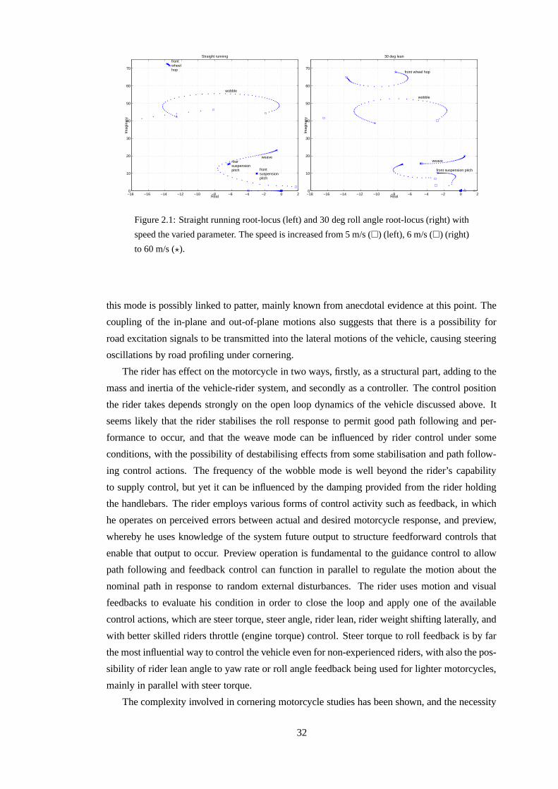
−18 −16 −14 −12 −10 −8 −6 −4 −2 0 20
10
20
30
40
50
60
70
Straight running
Real
Imag
inar
y
wobble
weave
front suspensionpitch
rear suspensionpitch
frontwheelhop
−18 −16 −14 −12 −10 −8 −6 −4 −2 0 20
10
20
30
40
50
60
70
30 deg lean
Real
Imag
inar
y
wobble
front wheel hop
weave
front suspension pitch
Figure 2.1: Straight running root-locus (left) and 30 deg roll angle root-locus (right) with
speed the varied parameter. The speed is increased from 5 m/s (�) (left), 6 m/s (�) (right)
to 60 m/s (?).
this mode is possibly linked to patter, mainly known from anecdotal evidence at this point. The
coupling of the in-plane and out-of-plane motions also suggests that there is a possibility for
road excitation signals to be transmitted into the lateral motions of the vehicle, causing steering
oscillations by road profiling under cornering.
The rider has effect on the motorcycle in two ways, firstly, as a structural part, adding to the
mass and inertia of the vehicle-rider system, and secondly as a controller. The control position
the rider takes depends strongly on the open loop dynamics of the vehicle discussed above. It
seems likely that the rider stabilises the roll response to permit good path following and per-
formance to occur, and that the weave mode can be influenced by rider control under some
conditions, with the possibility of destabilising effects from some stabilisation and path follow-
ing control actions. The frequency of the wobble mode is well beyond the rider’s capability
to supply control, but yet it can be influenced by the damping provided from the rider holding
the handlebars. The rider employs various forms of control activity such as feedback, in which
he operates on perceived errors between actual and desired motorcycle response, and preview,
whereby he uses knowledge of the system future output to structure feedforward controls that
enable that output to occur. Preview operation is fundamental to the guidance control to allow
path following and feedback control can function in parallel to regulate the motion about the
nominal path in response to random external disturbances. The rider uses motion and visual
feedbacks to evaluate his condition in order to close the loop and apply one of the available
control actions, which are steer torque, steer angle, rider lean, rider weight shifting laterally, and
with better skilled riders throttle (engine torque) control. Steer torque to roll feedback is by far
the most influential way to control the vehicle even for non-experienced riders, with also the pos-
sibility of rider lean angle to yaw rate or roll angle feedback being used for lighter motorcycles,
mainly in parallel with steer torque.
The complexity involved in cornering motorcycle studies has been shown, and the necessity
32
of automated methods in the analysis of such systems has been demonstrated. Several multibody
modelling tools exist which are capable of fulfilling this task. These can be employed in order
to further advance knowledge and understanding of the subject.
33
Part II
Motorcycle Models
34
The use of automated methods for generating equations of motion and for the analysis of
motorcycle dynamics is demonstrated in the following chapters. The multibody platform used
is AUTOSIM. Three different motorcycle models are presented in order of complexity, one in
each of the next three chapters. The first two models are reproductions of hand-derived mod-
els (Sharp, 1971, 1994b) and are presented in detail in a tutorial fashion in Chapters 3 and 4
respectively. This work is based on internal reports (Evangelou and Limebeer, 2000a,b). The
third model is based on previous work by (Sharp and Limebeer, 2001) and an overview of that
work is given in Chapter 5 together with some improvements. In Chapter 6 animation meth-
ods of the same model are presented, based on an internal report (Evangelou and Limebeer,
2001). All the computer files that will be mentioned are available for download from the web-
site http://www.ee.ic.ac.uk/control/motorcycles/ and the various AUTOSIM commands used are
explained in Appendix B. For further help with AUTOSIM the reference manual (Anon., 1998)
can be consulted.
35
Chapter 3
The Sharp 1971 motorcycle model
3.1 Physical description of the model
The following assumptions are made regarding the representation of the vehicle (Sharp, 1971):
1. The vehicle consists of two rigid frames that are joined together via a conventional steering
mechanism. This steering freedom is constrained by a linear steering damper.
2. The front frame consists of the front wheel, forks, handlebars and fittings.
3. The rear frame consists of the main structure, the engine-gearbox assembly, the petrol
tank, seat, rear swinging arm, the rear wheel and a rigidly attached rider.
4. Each frame has a longitudinal plane of symmetry and the axis through the front frame
mass centre parallel to the steering axis is a principal axis.
5. The road wheels are rigid discs each of which makes point contact with the road. They
roll without longitudinal slip on a flat level road surface.
6. The axis of rotation of the engine flywheel is transverse.
7. The machine moves at constant forward speed with freedom to side slip, yaw, and roll;
only small perturbations from straight running are considered.
8. The air through which the machine moves is stationary and the effects of aerodynamic
side forces, yawing moments and rolling moments will be small compared with the tyre
effects and are therefore neglected. The effects of drag, lift and pitching moment are to
modify the vertical loading of the tyres and to make necessary a longitudinal force at the
driving wheel sufficient to maintain the assumed constant forward speed. These effects
are accounted for by variations in the coefficients relating tyre side forces to side-slip and
camber angles.
9. Pneumatic trail of the tyres is not considered since, for the rear tyre, its effect will be very
small, and for the front tyre it is small compared with the mechanical trail.
36
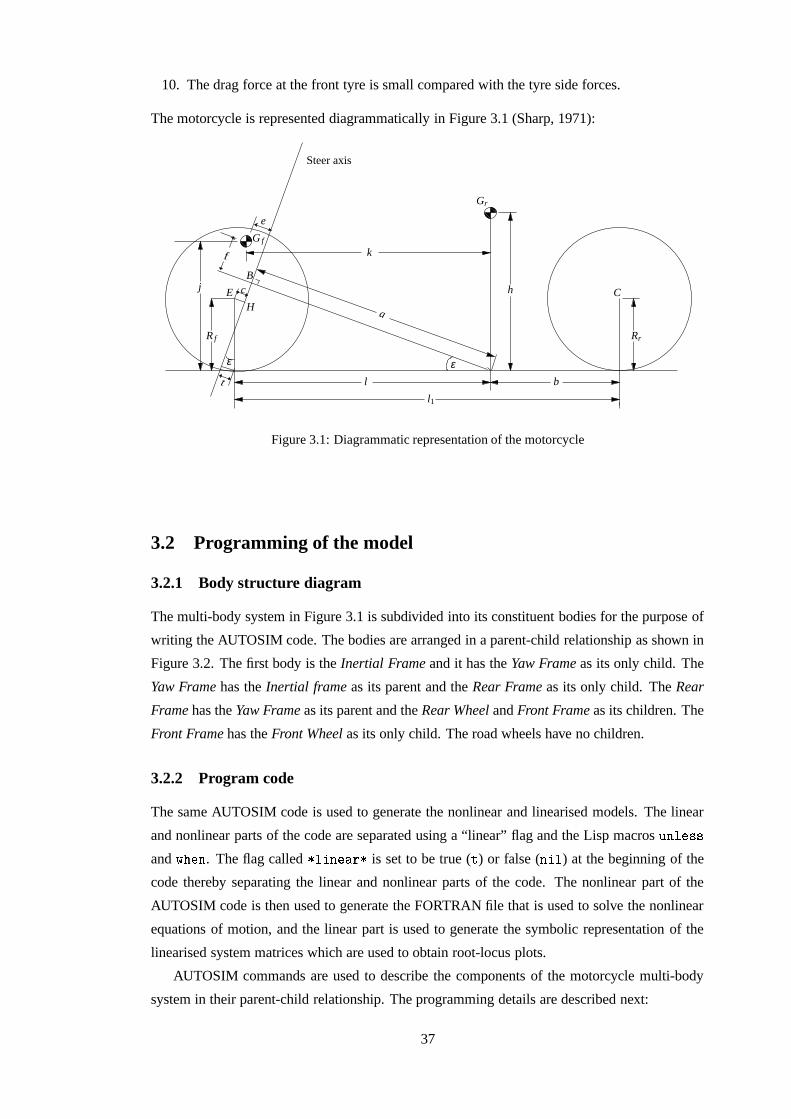
10. The drag force at the front tyre is small compared with the tyre side forces.
The motorcycle is represented diagrammatically in Figure 3.1 (Sharp, 1971):
Steer axis
f
PSfrag replacements
k
a
ε ε
Gr
G f
j
bl
C
B
EH
c
R f
t
l1
h
Rr
e
Figure 3.1: Diagrammatic representation of the motorcycle
3.2 Programming of the model
3.2.1 Body structure diagram
The multi-body system in Figure 3.1 is subdivided into its constituent bodies for the purpose of
writing the AUTOSIM code. The bodies are arranged in a parent-child relationship as shown in
Figure 3.2. The first body is the Inertial Frame and it has the Yaw Frame as its only child. The
Yaw Frame has the Inertial frame as its parent and the Rear Frame as its only child. The Rear
Frame has the Yaw Frame as its parent and the Rear Wheel and Front Frame as its children. The
Front Frame has the Front Wheel as its only child. The road wheels have no children.
3.2.2 Program code
The same AUTOSIM code is used to generate the nonlinear and linearised models. The linear
and nonlinear parts of the code are separated using a “linear” flag and the Lisp macros ������ � �
and � � � � . The flag called ������ � � is set to be true ( � ) or false ( �
���) at the beginning of the
code thereby separating the linear and nonlinear parts of the code. The nonlinear part of the
AUTOSIM code is then used to generate the FORTRAN file that is used to solve the nonlinear
equations of motion, and the linear part is used to generate the symbolic representation of the
linearised system matrices which are used to obtain root-locus plots.
AUTOSIM commands are used to describe the components of the motorcycle multi-body
system in their parent-child relationship. The programming details are described next:
37
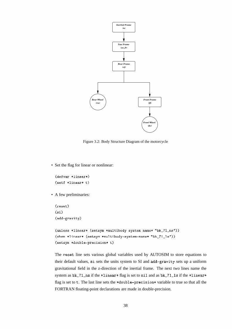
Yaw Frame
(rf)Rear Frame
Rear Wheel (rw)
Front Frame (ff)
Front Wheel(fw)
(ya_fr)
Inertial Frame(n)
Figure 3.2: Body Structure Diagram of the motorcycle
• Set the flag for linear or nonlinear:
������������� ���������������������� ��������������
• A few preliminaries:
����������������������������� ���������!��
�#"��� ������$� ����������%�&������'!'()��(�"� �����*�+���!����'!��'���,(-�.���,(����0/�*�1�2�3�4'25����/�����#6�7����8� ����������%��������'!5(%��(�"� �����*�+���!����,!��'���,(9������(����0/�*�1�2�3�4'2� ���/�����������,!5()�5��+�"�*� �����:����;������'+����<���
The � � � � � line sets various global variables used by AUTOSIM to store equations to
their default values, � � sets the units system to SI and >=�? � �@ � ��A sets up a uniform
gravitational field in the z-direction of the inertial frame. The next two lines name the
system as B�C ��D-E�� � � if the ������ � � flag is set to �
���and as B�C ��D>E�� � � if the �
����� � �
flag is set to � . The last line sets the � �F � B ��� =�G � �IH�� � � F � � variable to true so that all the
FORTRAN floating-point declarations are made in double-precision.
38
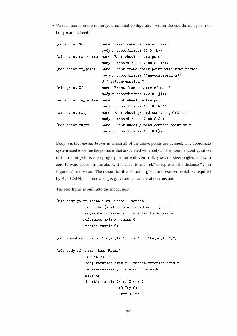
• Various points in the motorcycle nominal configuration within the coordinate system of
body n are defined:
���������.:�+��������� � ���,(��8/������ �����(�� ;���������$+�� (�������/� *�+���!$����;�+�+��������������������� ��7I���
���������.:�+������ �6�2�;5��������� ���,(��8/������ 6�7����� ;��������� :�+������I/� *�+���!$����;�+�+�����������������.��*�*� ��������
���������.:�+������0����2 ��+������ � ���,(��8/����+���� ����,(�����+��.���$:�+������ 6��,��7 ���� ����,(���/� *�+���!$����;�+�+�����������������,/,������;�+��-���5:����� �+5�I��/�)/��5����������� ����:����� �+�����/����
���������.:�+���������� � ���,(��8/����+���� ����,(�� ;���������$+�� (�������/� *�+���!$����;�+�+������������������1�1�8��� �����
���������.:�+������0�6�2�;5��������� ���,(��8/����+���� 6�7����� ;��������� :�+��.���9/� *�+���!$����;�+�+����������������� � ��8���������
���������.:�+������ �6�;,:�� � ���,(��8/������ 6�7����� 0 ��+�"���� ;�+�������;'�0:�+��.���8��� �-/� *�+���!$����;�+�+�����������������.��*�*�������
���������.:�+������0�6�;,:�� � ���,(��8/����+���� 6�7����� ��+5"���� ;�+�������;'� :�+������ ��� �-/� *�+���!$����;�+�+����������������� � ��������
Body n is the Inertial Frame in which all of the above points are defined. The coordinate
system used to define the points is that associated with body n. The nominal configuration
of the motorcycle is the upright position with zero roll, yaw and steer angles and with
zero forward speed. In the above, it is usual to use “ B�B ” to represent the distance “ B ” in
Figure 3.1 and so on. The reason for this is that � , ? etc. are reserved variables required
by AUTOSIM; � is time and ? is gravitational acceleration constant.
• The rear frame is built into the model next:
���������.*�+���! !���2���� ���,(��8/�����6�����,(���/ � :����5��� �� �������� ������ ��� !�� ����+��������;�+�+������������� ���������� *�+��!��,�+�������5+5�I�5��������� � :����5�����,�+�������5+5�I�'���������� ����������;����5��������� � (��������� ���������5���&(������������
����������,:���������;�+����,���������� /.��" �#!���2�� ��4� � ��"9/!� " /.�" ��!���2���"��4��/�
���������.*�+���! ��#� ���,(�� /�����������,(���/� :��������0!���2��� *�+���!��,�+������'+��I�'��������� � :����������,�+������'+����5��������� ��������5��;����5�������<! ��;�(>��;5+�+����.������������ (������%$�� �.�������'���&(��������)����&, ����'� �(���
���)&,�!�����*'�+�+���,&,+�������
39
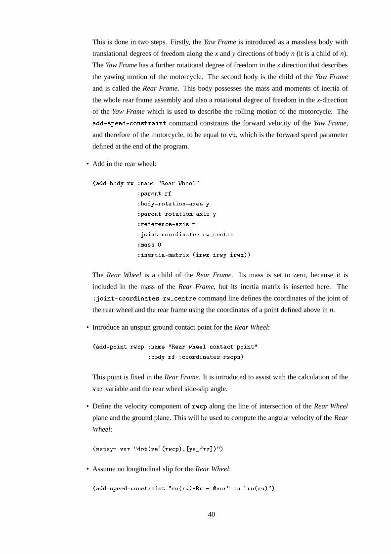
This is done in two steps. Firstly, the Yaw Frame is introduced as a massless body with
translational degrees of freedom along the x and y directions of body n (it is a child of n).
The Yaw Frame has a further rotational degree of freedom in the z direction that describes
the yawing motion of the motorcycle. The second body is the child of the Yaw Frame
and is called the Rear Frame. This body possesses the mass and moments of inertia of
the whole rear frame assembly and also a rotational degree of freedom in the x-direction
of the Yaw Frame which is used to describe the rolling motion of the motorcycle. The >= �G ��� -= H F � ��� � � � � command constrains the forward velocity of the Yaw Frame,
and therefore of the motorcycle, to be equal to@� , which is the forward speed parameter
defined at the end of the program.
• Add in the rear wheel:
���������.*�+���! 6 � ���,(�� /������ � 7����� �/� :��������0��� *�+���!��,�+������'+��I�'�������<!� :����������,�+�������5+5���'�������<!� ��������5��;����5�������������+��������;�+�+�������������� �6�2�;��5������� (��������� �.�������'���&(��������)�.�,�6+� �,�6�!8�,�6+�����
The Rear Wheel is a child of the Rear Frame. Its mass is set to zero, because it is
included in the mass of the Rear Frame, but its inertia matrix is inserted here. The��� F � � � = H F�F� � � � � � � � � H � � ��� � command line defines the coordinates of the joint of
the rear wheel and the rear frame using the coordinates of a point defined above in n.
• Introduce an unspun ground contact point for the Rear Wheel:
���������.:�+������ �6�;,:#� ���,(��8/������� 6�7����� ;�+5������;'� :�+������I/� *�+���! �� ��;�+�+������������� 6�;,:��I�
This point is fixed in the Rear Frame. It is introduced to assist with the calculation of the@� � variable and the rear wheel side-slip angle.
• Define the velocity component of � � H G along the line of intersection of the Rear Wheel
plane and the ground plane. This will be used to compute the angular velocity of the Rear
Wheel:
��������,!5( ��"�)/���+�� ������ >���6�;,:�� ��� !���2���������/��
• Assume no longitudinal slip for the Rear Wheel:
����������,:���������;�+����,���������� /.�" �#�6I��� ������"�9/ � " /." ���6I��/�
40
The rotational speed of the Rear Wheel is constrained to be = @ � ������� which means that the
wheel is not allowed to slip longitudinally. The effect of this (nonholonomic) constraint
is to remove the rotational speed of the rear wheel as a freedom from the equations of
motion.
• Define the steering and reference axis for the Front Frame:
��������,!5()�'�������2������� /����.� ����:����� �+��I�� � ���� � 8;�+��-����:����� �+��I�� � �� � ��/���������,!5(��6�2���������5��;�� /�;�+��-����:����� +��I��� � �� ���$� ����� ����:����� +��I��� � �� � ��/�
These two axes are defined to assist the addition of the front frame assembly.
• Add in the Front Frame:
���������.*�+���!$���#� ���,(�� /����+����������(���/� :��������0��� *�+���!��,�+������'+��I�'���������� :����������,�+�������5+5���'������� ���'�������2�������� ��������5��;����5������� ���6�25�����������;������+��������;�+�+�������������� ����2 ��+��������;&(>��;�+�+�������������������� (������%$��� �.�������'���&(��������)��&'� �,&'�! &,�+�����
The Front Frame is a child of the Rear Frame. It has one degree of freedom, that is a steer-
ing freedom about the steering axis ( ��� ��� ��� �� � � ). The reference axis (�� �� �
� � � � � H � )
is used to define the nominal configuration of the Front Frame.
• Add in the Front Wheel:
���������.*�+���!$��6 � ���,(�� /����+���� � 7����� �/� :�������� ���� *�+���!��,�+������'+��I�'�������<!� :����������,�+�������5+5���'�������<!� ��������5��;����5�������������+��������;�+�+�������������� �6�2�;��5������� (��������� �.�������'���&(��������)�.�'�6+� �'�6�!8�'�6+�����
This body has the Front Frame as parent. Its mass is zero since this has been included in
the mass of the Front Frame, but its moments of inertia are not and so they are inserted
here.
• Introduce an unspun ground contact point for the Front Wheel:
���������.:�+������0�6�;,:#� ���,(��8/����+5��� 6�7����� ;�+�������;'� :�+������9/� *�+���! ��� ��;�+�+������������� ��6�;,:��I�
41
This point is fixed in the Front Frame. It is introduced to assist with the calculation of the@��
variable and the Front Wheel side-slip angle.
• Define the velocity component of��H G along the line of intersection of the Front Wheel
plane and the ground plane:
��������,!5(��6�2� ��%/����, ���:� ��5��� � � ���!�� ��� �(� ������/5���������,!5(��6�2� +��� 8/�;,�+����-�����6�2� ��"��� �+� ����/����������,!5( ��"��%/���+�� ������ >���6�;,:�� �����6�2� �+'�� ���/��
The second line, which makes use of the first, defines the direction of the line of inter-
section of the Front Wheel plane and the ground plane. The last line finds the velocity
component of��H G in the direction of
�� � � F � ? .
• No longitudinal slip on the Front Wheel:
����������,:���������;�+����,���������� /.�" ���6I��� ��� ����"��I/ � " /." ���6I��/�
As with the Rear Wheel, it is assumed that the Front Wheel undergoes no longitudinal slip.
Consequently, its angular velocity is set to = @ � � ��� � and the rotational speed of this wheel
as a freedom is eliminated from the equations of motion by AUTOSIM.
• Define the camber and side-slip angles:
��������,!5( :�7I�,)/,������� ����+� � � �(� � � � ���!�������/��
��������,!5( :�7I�'�%/,������� ����+� � � �(� � � � ����!�������/��
��������,!5( �� 5:�7��%/,�����.� ����+� � � !���2���!�� ������ ������ �#6�;,:I�������/�
��������,!5( �� 5:�7����8/,�����.� ����+� � ���6�2� ��"� ���� �#���� -����6�;�:I�������/��
These angles are needed in the calculation of the side forces. The first line defines the
Rear Wheel camber angle, the second line defines the Front Wheel camber angle and the
third line defines the Rear Wheel side-slip angle by making use of the point � � H G defined
above. The last line defines the Front Wheel side-slip angle via the point��H G . Note that
for the side-slip angles, positive lateral velocities give positive slip values and negative
forces. As a consequence the signs of the side-slip angles in the side force expressions
below are opposite to those in the original paper (Sharp, 1971).
• Introduce a steering head damping torque:
��������� (�+,(������ �5� � ���,(�� /������������� ����,(�:I���� 9/� *�+��!94 ��� � *�+���!��0��� ���,���;'���5+5� � ��� � �� (�� �I�,��"���� /�����'�" ������� ��'��2�����/��
42
This torque acts on the Front Frame with a positive magnitude and on the Rear Frame with
negative magnitude in the z-direction of the Front Frame. Its magnitude is proportional
to the rotation speed of the Front Frame relative to the Rear Frame. There is also a
contribution from the rider ( � � ���� ) which defaults to zero.
• Work out the tyre side forces and introduce a simple tyre relaxation model:
����������'��������,�����'�5*� �� ������2��+�������������'��"(�����,��������,�����.�%���2��+��%/�� ���"�������, '(������9��� '��4�� ���� ':�7�� '����� ��:�7��,�������/��
����������'��������,�����'�5*� �� ��������2��+�������������'��"(�����,��������,�����.�%����2��+��%/�� ���"��������, '(��������9��� '���4�� ���� ':�7���� '�� ��� ��:�7��'����������/��
The �-= ��� � � = @ � � B ��� commands introduce two state variables, one for each of
the two force expressions, that are used to describe the tyre relaxation property. The
force equations are defined with the � � �>= � � = � � � � =� � � ��@ and use the values of the
side-slip and camber angles defined above; the � � �>= � � = ��� � � = � � ��@ complements the >= � � � � � F � command in earlier versions of AUTOSIM, overcoming a difficulty aris-
ing previously with added variables in forming the linear model. Notice the minus sign on
the � � E ��� �� G � � and � � E ��� �� G � � terms.
• Introduce the tyre side forces:
���������5 ��������,��+�;�� ���� � ���,(�� /������ � 7����� �������� ���!��� ��+�;���/� ���,���;'���5+�� � !���2���!��� :�+������94<�6�;,:� (�� ��I�,�"���� ����
���������5 ��������,��+�;�� ��� � � ���,(�� /����+���� � 7����� �������� ���!������+�;���/� ���,���;'���5+�� ��6�2� ����� :�+������94 �6�;,:� (�� ��I�,�"���� �����
The direction of the two tyre side forces is in the ground plane and normal to the line of
intersection of the ground plane and the wheel plane.
• Incorporate the normal tyre loads:
��������,!5( ��+�"�����2�����;'��+ /�:�+��9���6�;,:�� �#�6�;�:��I��/5���������,!5( ���2�����;'��+ /�:�+��9�*��"�#6�;,:��I��/����������,!5( ����2�����;'��+ /�:�+��9�*��� �#6�;,:��I��/��
��������,!5(����%/� ���9��$����5��+� � � ����2�����;,��+ ��� �+� ��� �$���'��+� � � ��2�����;���+� ��� �(� ��������+�� � � ��+�"�����25����;,��+�"��� �(� ����/�
43
���������5 ��������,��+�;�� �����#� ���,(�� / � �������;��� �+���� +�� ���+����$6�7����� �/� ���,���;'���5+�� � � � �� :�+������94 �6�;,:� (�� ��I�,�"���� � �����
The first three lines define three vectors from the rear wheel ground contact point to three
points in the nominal configuration. These points are the front wheel ground contact point,
the rear frame centre of gravity and the front frame centre of gravity respectively. The next
line calculates the magnitude of the normal force on the front wheel by projecting the three
vectors onto the ground plane in the nominal configuration and taking moments about the
rear wheel contact point. The >= � � � � = � F � H � command introduces the normal force
into the vehicle equations of motion. Note that only the front force is influential since the
system has no heave freedom in body n and therefore the rear force is omitted.
• Derive the equations of motion of the system or the linearised equations:
�#"��� ������$� ����������%����!����,(-��;�������#6�7����8� �������������������������5�5*� ���� ��!������� ����� �'��2������� ���������� "8�'��2�� ����
If the �� ���� � � flag is set to �
���the full equations of motion are derived. Alternatively
if the flag is set to � the linearised equations are derived with � � ���� as the input. ��� � � �is defined as a real variable that is used as a steering torque input from the rider, and
therefore the corresponding B-Matrix is also computed in the linearised equations.
• All the motorcycle parameters are introduced with their names and default values1:
��� ��������"� �� ���� 5"���� ��+ (������������������.���,(���� $�� /�$������0+�� ���+���� ����,(���/
$� /�$������0+��$���� �����(���/���������,��������"� �����$���� ������3 ��$� ��4,3��� �� ���
��� ��������"� �� ���� 5"���� ��+ (�+,(�������� +��8���������5���������.���,(���� &'� � /����+���� �����(������������5� 6�� �� �������� ��*�+5"�� (������ ;��5�������/
&'��! /����+���� �����(������������5� 6�� �� �������� ��*�+5"�� (������ ;��5�������/&'�+� /����+���� �����(������������5� 6�� �� ����� �� ��*�+5"�� (������ ;��5�������/&,+� /.���� ����,(�� �.�������'� 6�� �� ������� � ��*�+�"�� (������ ;����������/&,�! /.���� ����,(�� �.�������'� 6�� �� ������� � ��*�+�"�� (������ ;����������/
1As can be seen from the sign of ������� , AUTOSIM uses the opposite sign convention for products of inertia
(−∑mixizi) as compared with (Sharp, 1971) (∑mixizi).
44
&,(� /.���� ����,(�� �.�������'� 6�� �� ����� � � ��*�+�"�� (������ ;����������/'�+�(�%/.���� ����,(�� �.�������'� :��+��"�;'�06�� �� ��� (������ ;5���������/�'�6(�)/����+���� 6�7����� ;��,(�*��� ���������5��/�'�6�!)/����+���� 6�7����� :�+� �� (�+,(������ +�%���������5��/�,�6(�)/.����$6�7����� ;5�,(�*�� �.�������'��/�,�6�!)/.����$6�7����� :�+� �� ���������5��/�
��������,��������"� �����&'� � 4 � ����� � &'��!��,&,�+������� � �&,+����4 ��4 � � � &,�!�)&,(���4 ����� ���'�+�(� ��4 �#3����� �'�6(��� �'�6�!����#3�4 � � �,�6+�� �,�6�! 4 �����+� � �
��� ����+�(������; :����,(����������������.���,(������� / ����� 6�7����� 0������."���/
��� / ���+���� 6�7����� ������"���/����������,��������"� ���� ��� � �� � � *�* ���3 � � 7 �����4�� �������������� �� � �������� �� � �
��:����� +�� �3�4 ������� � � ����� ���3�4�� 1�1 � � � ��� � ���$ � ������������ � �
��� ��!��� :����,(���������������.���,(���� ���, 5(���%/.���� ��!��� ��� ���������5+�� ����� ���7-/
���, 5(���8/����+����$��!��� ��� ��������'+�� ��5�� ���7-/'��I4 /����+����$��!��� ;�+�������� �'���'�����������/'���� /����+����$��!��� ;��,(�*����'���,�����������/'�94 /.���� ��!��� ;�+���������� �'���'������������/'� � /.���� ��!��� ;��,(�*�����'���'������������/��
��������,��������"� ���� ���, 5(������� ���� � ����, 5(�������� ���'���4 4�4�4,3��� � � '���� ��� � ���4��� '�944�� � ��4 � � ������'� �84�� ��� �� ��� ���
��� ����7�� :�����(���������������.���,(���� � /��,�������.�� $���,(�:I���� �;�+���������;��5�����9/����������,��������"� ���� � ��� 3 � ��" � ��4���� � ��#"��� ������$� ����������%�&������'��������"� 5���0�.:�������%4 �'��+5:����+� �'����:������4 /��� �������/
� ���+���$��:��5��� 4,���53 �'��2����������
The last line sets some default values relevant only to the nonlinear model.
• Write up files:
�#"��� ������$� �����������#6���,�����,��+��,���� �� 6���,���������&( /�*�1�2�3�4'25��� � �I/��#6���,�����,��+��,���� �� :���������'��������"� ����.:�+����.���'+5��� /�:�+��������5+���� � �+���9/5��#6���,�����,��+��,���� �� :���������'��������"� ����,���,���;'���'+5���0/��������;'���'+���� � � ���9/���#6���,�����,��+��,���� �� :����������:����,(�������� /�:�����(������� � �+����/���#6�7����8� �����������#6���,�����,��+��,���� �� 6���,�����&(���� ���*�/�*�1�2�3�4'2� �� � ( /��
The FORTRAN file is written to B�C ��D-E � � ��� � and the files G�F � � � � F � ��� � � � , � � ��H � � F � �� � � �
45
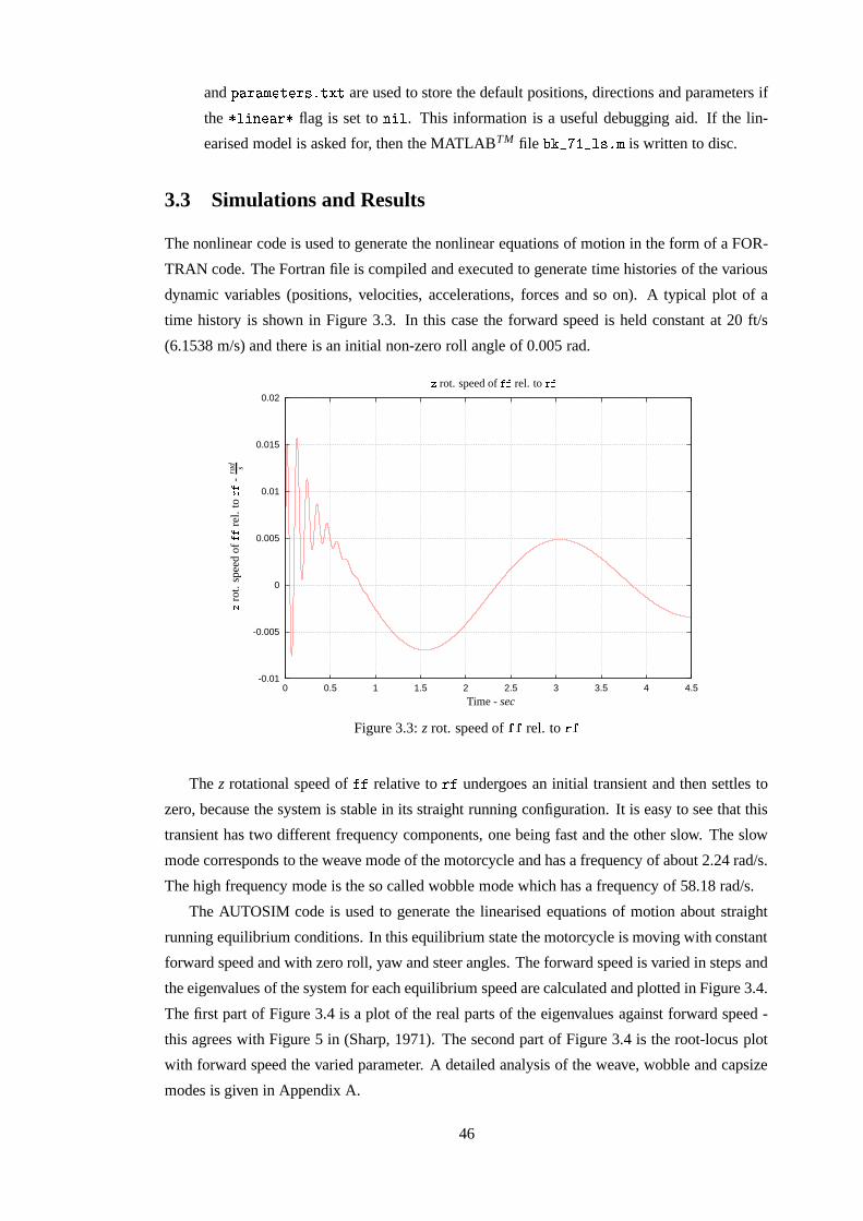
and G � �� � � � � ��� � � � are used to store the default positions, directions and parameters if
the ������ � � flag is set to �
� �. This information is a useful debugging aid. If the lin-
earised model is asked for, then the MATLABTM file B�C ��D>E�� � �� � is written to disc.
3.3 Simulations and Results
The nonlinear code is used to generate the nonlinear equations of motion in the form of a FOR-
TRAN code. The Fortran file is compiled and executed to generate time histories of the various
dynamic variables (positions, velocities, accelerations, forces and so on). A typical plot of a
time history is shown in Figure 3.3. In this case the forward speed is held constant at 20 ft/s
(6.1538 m/s) and there is an initial non-zero roll angle of 0.005 rad.
-0.01
-0.005
0
0.005
0.01
0.015
0.02
0 0.5 1 1.5 2 2.5 3 3.5 4 4.5
PS
fragreplacem
ents
� rot. speed of ��� rel. to ���
� rot.
spee
dof
�� rel.
to
� -ra
d s
Time - sec
Figure 3.3: z rot. speed of � rel. to �
The z rotational speed of ��� relative to ��� undergoes an initial transient and then settles to
zero, because the system is stable in its straight running configuration. It is easy to see that this
transient has two different frequency components, one being fast and the other slow. The slow
mode corresponds to the weave mode of the motorcycle and has a frequency of about 2.24 rad/s.
The high frequency mode is the so called wobble mode which has a frequency of 58.18 rad/s.
The AUTOSIM code is used to generate the linearised equations of motion about straight
running equilibrium conditions. In this equilibrium state the motorcycle is moving with constant
forward speed and with zero roll, yaw and steer angles. The forward speed is varied in steps and
the eigenvalues of the system for each equilibrium speed are calculated and plotted in Figure 3.4.
The first part of Figure 3.4 is a plot of the real parts of the eigenvalues against forward speed -
this agrees with Figure 5 in (Sharp, 1971). The second part of Figure 3.4 is the root-locus plot
with forward speed the varied parameter. A detailed analysis of the weave, wobble and capsize
modes is given in Appendix A.
46
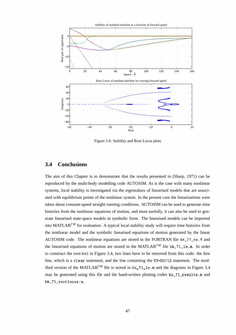
0 20 40 60 80 100 120 140 160
−15
−10
−5
0
−50 −40 −30 −20 −10 0 10
−60
−40
−20
0
20
40
60
PSfrag replacements
Stability of standard machine as a function of forward speed
Rea
lpar
tof
eige
nval
ue
Speed - f ts
Root Locus of standard machine for varying forward speed
Imag
inar
y
Real
Figure 3.4: Stability and Root Locus plots
3.4 Conclusions
The aim of this Chapter is to demonstrate that the results presented in (Sharp, 1971) can be
reproduced by the multi-body modelling code AUTOSIM. As is the case with many nonlinear
systems, local stability is investigated via the eigenvalues of linearised models that are associ-
ated with equilibrium points of the nonlinear system. In the present case the linearisations were
taken about constant-speed straight running conditions. AUTOSIM can be used to generate time
histories from the nonlinear equations of motion, and most usefully, it can also be used to gen-
erate linearised state-space models in symbolic form. The linearised models can be imported
into MATLABTM for evaluation. A typical local stability study will require time histories from
the nonlinear model and the symbolic linearised equations of motion generated by the linear
AUTOSIM code. The nonlinear equations are stored in the FORTRAN file B�C���D>E�� � �� � and
the linearised equations of motion are stored in the MATLABTM file B�C���D-E � � �� � . In order
to construct the root-loci in Figure 3.4, two lines have to be removed from this code: the first
line, which is aH����� � statement, and the line containing the ��������� �-E� statement. The mod-
ified version of the MATLABTM file is stored in B�C ��D-E�� � ��� � and the diagrams in Figure 3.4
may be generated using this file and the hand-written plotting codes B�C ��D-E�� � � � � � � ��� � and
B�C���D>E���IF�F � � F H � �� � .
47
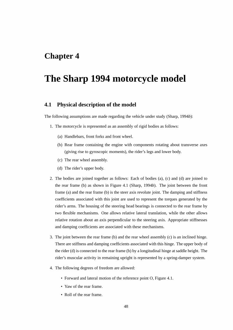
Chapter 4
The Sharp 1994 motorcycle model
4.1 Physical description of the model
The following assumptions are made regarding the vehicle under study (Sharp, 1994b):
1. The motorcycle is represented as an assembly of rigid bodies as follows:
(a) Handlebars, front forks and front wheel.
(b) Rear frame containing the engine with components rotating about transverse axes
(giving rise to gyroscopic moments), the rider’s legs and lower body.
(c) The rear wheel assembly.
(d) The rider’s upper body.
2. The bodies are joined together as follows: Each of bodies (a), (c) and (d) are joined to
the rear frame (b) as shown in Figure 4.1 (Sharp, 1994b). The joint between the front
frame (a) and the rear frame (b) is the steer axis revolute joint. The damping and stiffness
coefficients associated with this joint are used to represent the torques generated by the
rider’s arms. The housing of the steering head bearings is connected to the rear frame by
two flexible mechanisms. One allows relative lateral translation, while the other allows
relative rotation about an axis perpendicular to the steering axis. Appropriate stiffnesses
and damping coefficients are associated with these mechanisms.
3. The joint between the rear frame (b) and the rear wheel assembly (c) is an inclined hinge.
There are stiffness and damping coefficients associated with this hinge. The upper body of
the rider (d) is connected to the rear frame (b) by a longitudinal hinge at saddle height. The
rider’s muscular activity in remaining upright is represented by a spring-damper system.
4. The following degrees of freedom are allowed:
• Forward and lateral motion of the reference point O, Figure 4.1.
• Yaw of the rear frame.
• Roll of the rear frame.
48
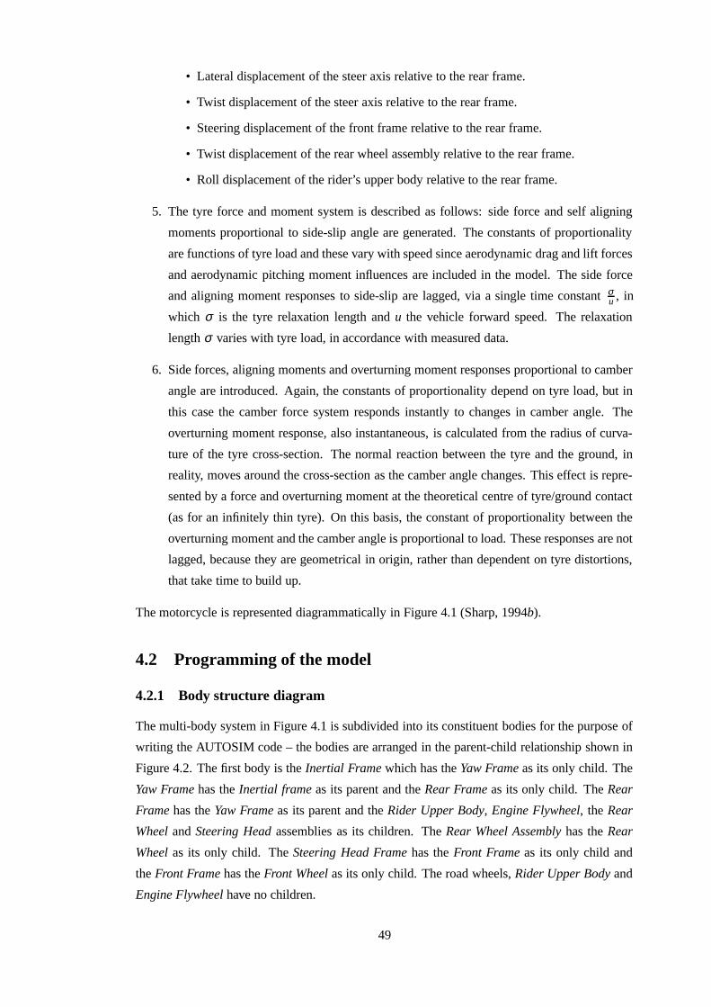
• Lateral displacement of the steer axis relative to the rear frame.
• Twist displacement of the steer axis relative to the rear frame.
• Steering displacement of the front frame relative to the rear frame.
• Twist displacement of the rear wheel assembly relative to the rear frame.
• Roll displacement of the rider’s upper body relative to the rear frame.
5. The tyre force and moment system is described as follows: side force and self aligning
moments proportional to side-slip angle are generated. The constants of proportionality
are functions of tyre load and these vary with speed since aerodynamic drag and lift forces
and aerodynamic pitching moment influences are included in the model. The side force
and aligning moment responses to side-slip are lagged, via a single time constant σu , in
which σ is the tyre relaxation length and u the vehicle forward speed. The relaxation
length σ varies with tyre load, in accordance with measured data.
6. Side forces, aligning moments and overturning moment responses proportional to camber
angle are introduced. Again, the constants of proportionality depend on tyre load, but in
this case the camber force system responds instantly to changes in camber angle. The
overturning moment response, also instantaneous, is calculated from the radius of curva-
ture of the tyre cross-section. The normal reaction between the tyre and the ground, in
reality, moves around the cross-section as the camber angle changes. This effect is repre-
sented by a force and overturning moment at the theoretical centre of tyre/ground contact
(as for an infinitely thin tyre). On this basis, the constant of proportionality between the
overturning moment and the camber angle is proportional to load. These responses are not
lagged, because they are geometrical in origin, rather than dependent on tyre distortions,
that take time to build up.
The motorcycle is represented diagrammatically in Figure 4.1 (Sharp, 1994b).
4.2 Programming of the model
4.2.1 Body structure diagram
The multi-body system in Figure 4.1 is subdivided into its constituent bodies for the purpose of
writing the AUTOSIM code – the bodies are arranged in the parent-child relationship shown in
Figure 4.2. The first body is the Inertial Frame which has the Yaw Frame as its only child. The
Yaw Frame has the Inertial frame as its parent and the Rear Frame as its only child. The Rear
Frame has the Yaw Frame as its parent and the Rider Upper Body, Engine Flywheel, the Rear
Wheel and Steering Head assemblies as its children. The Rear Wheel Assembly has the Rear
Wheel as its only child. The Steering Head Frame has the Front Frame as its only child and
the Front Frame has the Front Wheel as its only child. The road wheels, Rider Upper Body and
Engine Flywheel have no children.
49
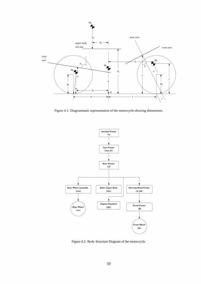
PSfrag replacements
bb
a
Mr
Mb
Mp
M f
j
b l
hs
hb
bp
hp
s
R f
t
hRr
e
εε1
twist axis
steer axis
upper body
roll axis
twist
axis
O
k
Figure 4.1: Diagrammatic representation of the motorcycle showing dimensions.
(efw)
Inertial Frame(n)
Yaw Frame(yaw_fr)
Rear Frame(rf)
Front Wheel(fw)
(ff)
Steering Head Frame
Front Frame
(st_hd)Rider Upper Body
(ubr)Rear Wheel Assembly
(rwa)
Rear Wheel(rw)
Engine Flywheel
Figure 4.2: Body Structure Diagram of the motorcycle.
50
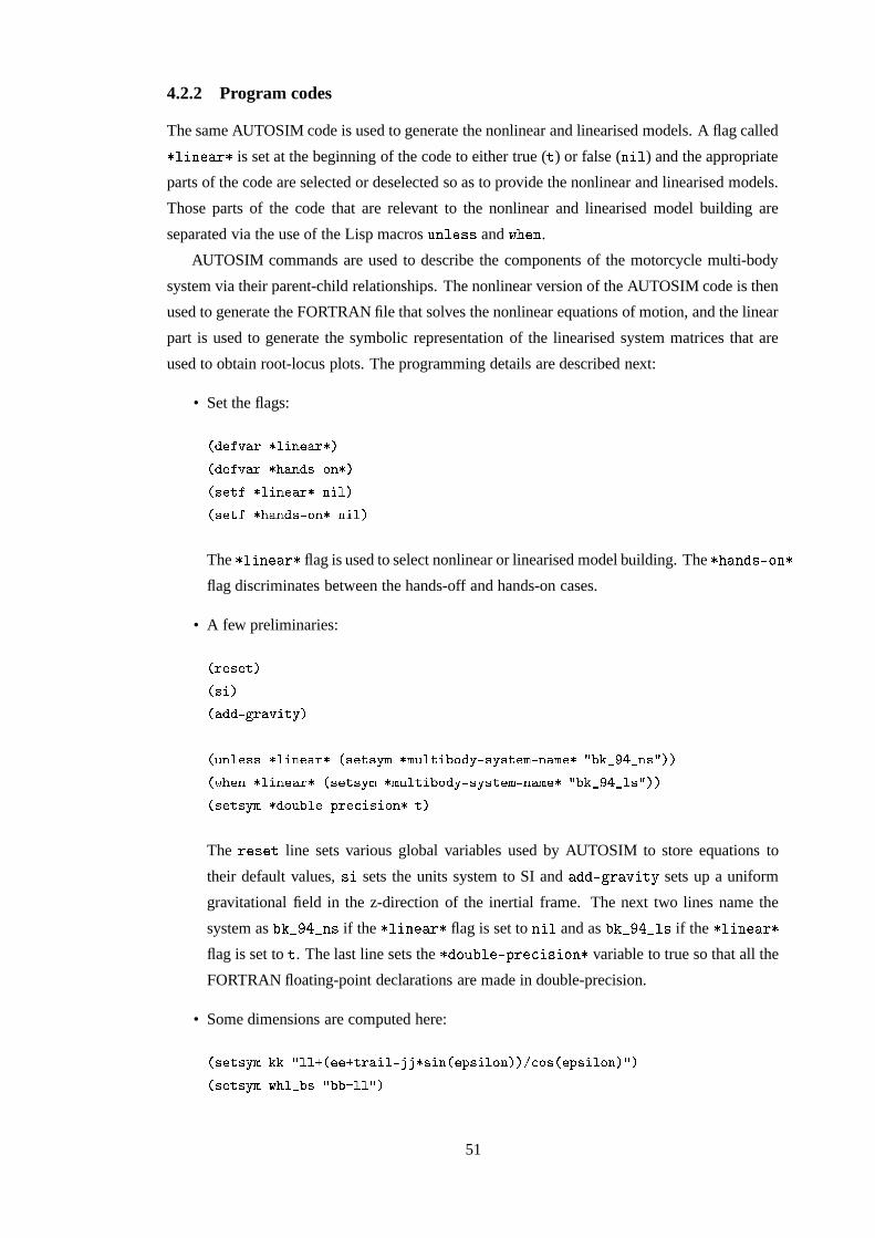
4.2.2 Program codes
The same AUTOSIM code is used to generate the nonlinear and linearised models. A flag called
������ � � is set at the beginning of the code to either true ( � ) or false ( �
� �) and the appropriate
parts of the code are selected or deselected so as to provide the nonlinear and linearised models.
Those parts of the code that are relevant to the nonlinear and linearised model building are
separated via the use of the Lisp macros ������ � � and � � � � .
AUTOSIM commands are used to describe the components of the motorcycle multi-body
system via their parent-child relationships. The nonlinear version of the AUTOSIM code is then
used to generate the FORTRAN file that solves the nonlinear equations of motion, and the linear
part is used to generate the symbolic representation of the linearised system matrices that are
used to obtain root-locus plots. The programming details are described next:
• Set the flags:
������������� �������������������������,7����������5+���������������� ���������� �I�� ������������,7����������'+���� ���� ��
The ������ � � flag is used to select nonlinear or linearised model building. The � � � ���=�F � �
flag discriminates between the hands-off and hands-on cases.
• A few preliminaries:
����������������������������� ���������!��
�#"��� ������$� ����������%�&������'!'()��(�"� �����*�+���!����'!��'���,(-�.���,(����0/�*�1�2 ���25����/�����#6�7����8� ����������%��������'!5(%��(�"� �����*�+���!����,!��'���,(9������(����0/�*�1�2 ���2� ���/�����������,!5()�5��+�"�*� �����:����;������'+����<���
The � � � � � line sets various global variables used by AUTOSIM to store equations to
their default values, � � sets the units system to SI and >=�? � �@ � ��A sets up a uniform
gravitational field in the z-direction of the inertial frame. The next two lines name the
system as B�C ����� � � � if the ������ � � flag is set to �
���and as B�C ����� � � � if the �
����� � �
flag is set to � . The last line sets the � �F � B ��� =�G � �IH�� � � F � � variable to true so that all the
FORTRAN floating-point declarations are made in double-precision.
• Some dimensions are computed here:
��������,!5( 1�1)/' � ����� �������� �� �+�������.� ���':����5 +��I�� ��;5+��-���':����5 �+5�I��/���������,!5( 6�7� �2'*�� /�*�* � � �/�
51
PSfrag replacements
p1
p2
p3
p4
p5p6
p7
p8
p9
p10 p11
p12
twist axis
steer axis
upper body
roll axis
twistaxis
O
Figure 4.3: Diagrammatic representation of the motorcycle showing points.
• Various points in the motorcycle nominal configuration within the coordinate system of
body n are defined (shown diagrammatically in Figure 4.3):
����������� ��������� ���������������� ����� ��� �"!#�#��� � �$ � ��%�%����&���(')�*��!+� � ������(����%���,-,.��/�/10�0
����������� ��������2 ���������������� �$3 /�����465�%�%+����& 4#'"!#�#��� � �$ ����%�%����&���(')�*��!+� � ������(����%����&�&�7+&",.�/�/ 7+&10�0
����������� ��������8 ����������� ��� #��� ��� ��� �9!#�+��� � �$ � ��%�%����&���(')�*��!+� � ������(����%���:(;�;",��+<�< 0�0
����������� ��������= ������������ �>��� � !#�#��� � �$ ����%�%����&���(')�*��!+� � ������(����%����&�&�7+�",?�#��/�/ 7�%���/�/ 7+�@�(0�0
����������� ��������A ���������������� �$3 /�����4-!#�#��� � �6�� ����@���&���(')�*��!+� � ������(����%����&�&9,���� � 0�0����������� ��������B ����������� ��� #��� 3 /�����4"!#�+��� � �6��������@���&���(')�*��!+� � ������(����%��C4�4$,���� 0�0����������� ��������D ���������������� �$3 /�����465�%�%+����& 4#'$<� �����$E1����/-����� ����� ��� � ���&���(')�*��!+� � ������(����%����(��&�&�F�����G�!#�%����+� %��#4##�@�#0��H,
�(�>����G�%���I���#� %��#4�#���+0��#0�0����������� ��������J ����������� ��� #���$K�E1��%>� ��� ��� �$<� ����$E1����/-����� �$��� ��� �����&���(')�*��!+� � ������(����%���>4�4#F�� � � �+4�L�!#�%@�M�#� %��#4(+� 0���%(%�G����+�I���>� %��+4�+�10��H,N��%�%�0�0����������� ��������O ������������ �>��� � <� �����$E1����/-����� �$��� ��� � ���&���(')�*��!+� � ������(����%����&�&�7+�",.�/�/ 7�%�0�0����������� ����������,P���������������� �$3 /�����46Q � +R����9!##������!>�)������������-���
��&���(')�*��!+� � ������(����%����&�&9,-, 0�0����������� �����������S����������� ��� #��� 3 /�����4TQ � #R����9!#+������!>�6�� �����.���-���
��&���(')�*��!+� � ������(����%��C4�4$,-, 0�0����������� ����������2P������������U��#��� � �$ � � ��%�%�R � � ���&���(')�*��!+� � ������(����%�����:#E�/ 4�7+& %#L�2 ��&�&@�V,���/�/�7�!��10�0
52
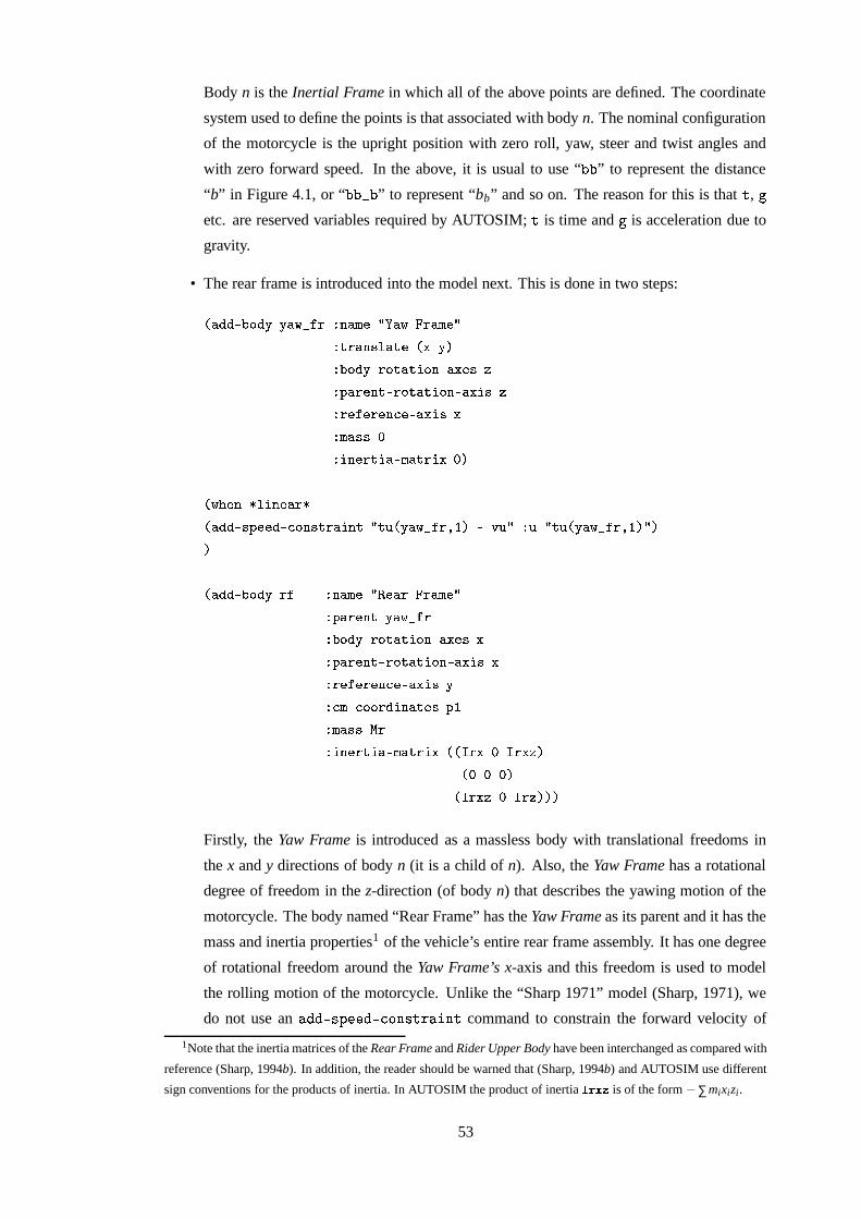
Body n is the Inertial Frame in which all of the above points are defined. The coordinate
system used to define the points is that associated with body n. The nominal configuration
of the motorcycle is the upright position with zero roll, yaw, steer and twist angles and
with zero forward speed. In the above, it is usual to use “ B�B ” to represent the distance
“b” in Figure 4.1, or “ B�B���B ” to represent “bb” and so on. The reason for this is that � , ?etc. are reserved variables required by AUTOSIM; � is time and ? is acceleration due to
gravity.
• The rear frame is introduced into the model next. This is done in two steps:
���������.*�+���! !���6�2���� ���,(�� /�����6�����,(���/� ��������� �����)��� !��� *�+���!����+������5+��I�5���������� :����������,�+������5+����5��������� �����������;����'���������� (�������������������5���&(�������������
�#6�7����8� ��������������������,:���������;�+����,���������� /.��" �#!���6�2�"��4� � �"-/ � " /���" ��!��56�2��"�.4��/��
���������.*�+���! �� � ���,(��8/������������,(���/� :��������$!���6�2��� *�+���!��,�+������'+��I�5���������� :����������,�+�������5+��I�,��������� ��������5��;����5������� !��;&(>��;�+�+���������������<:-4� (������ $�� �.�������'���&(�������� ����&,+���)&,+�+���
�����������&, �(���,&,+�������
Firstly, the Yaw Frame is introduced as a massless body with translational freedoms in
the x and y directions of body n (it is a child of n). Also, the Yaw Frame has a rotational
degree of freedom in the z-direction (of body n) that describes the yawing motion of the
motorcycle. The body named “Rear Frame” has the Yaw Frame as its parent and it has the
mass and inertia properties1 of the vehicle’s entire rear frame assembly. It has one degree
of rotational freedom around the Yaw Frame’s x-axis and this freedom is used to model
the rolling motion of the motorcycle. Unlike the “Sharp 1971” model (Sharp, 1971), we
do not use an �-= ��G ��� -= H F � ����� � � � command to constrain the forward velocity of
1Note that the inertia matrices of the Rear Frame and Rider Upper Body have been interchanged as compared with
reference (Sharp, 1994b). In addition, the reader should be warned that (Sharp, 1994b) and AUTOSIM use different
sign conventions for the products of inertia. In AUTOSIM the product of inertia � ����� is of the form −∑mixizi.
53
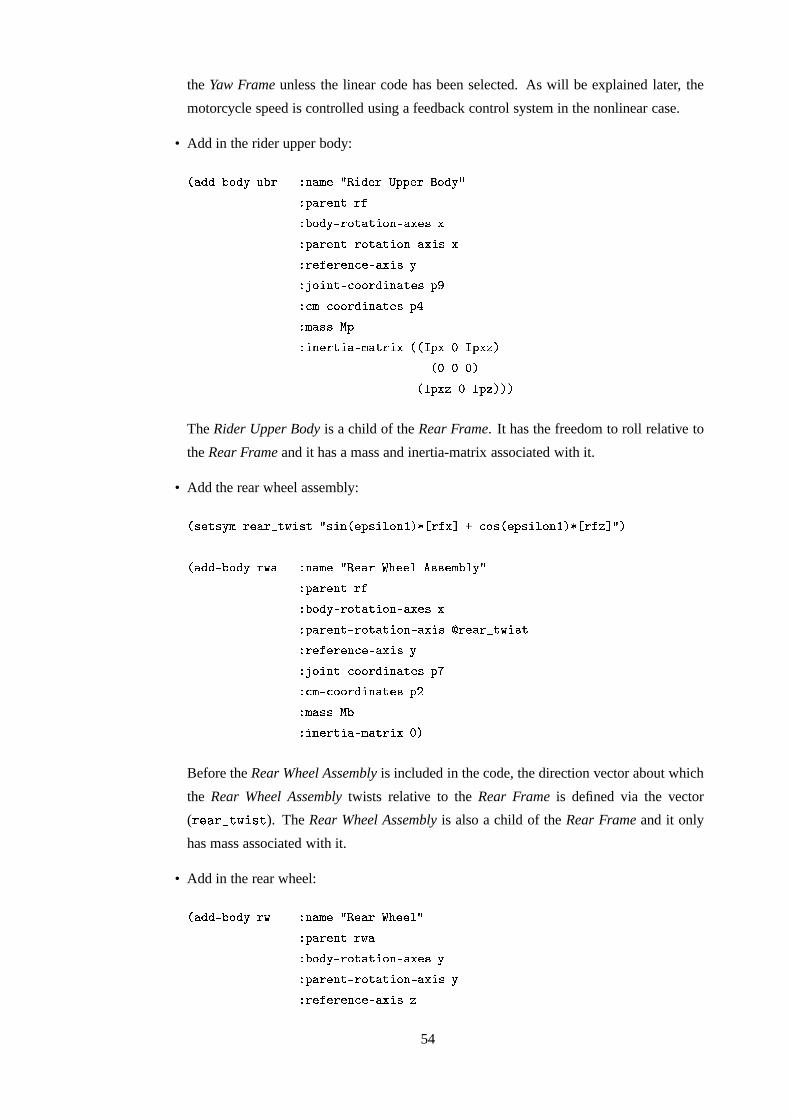
the Yaw Frame unless the linear code has been selected. As will be explained later, the
motorcycle speed is controlled using a feedback control system in the nonlinear case.
• Add in the rider upper body:
���������.*�+���!0"�*� � ���,(��8/����'������:�:������+���!9/� :��������$��� *�+���!��,�+������'+��I�5���������� :����������,�+�������5+��I�,��������� ��������5��;����5������� !����+��������;�+�+������������� : ���;&(>��;�+�+���������������<: � (������ $�:� �.�������'���&(�������� ����&�:(���)&�:(�+���
�����������&�:+�(���,&�:(�������
The Rider Upper Body is a child of the Rear Frame. It has the freedom to roll relative to
the Rear Frame and it has a mass and inertia-matrix associated with it.
• Add the rear wheel assembly:
��������,!5( �����2���6I���,� /����.� ����:����� �+��-4���� � ������ ;�+��-���5:����� �+5�-4��� � �� � ��/�
���������.*�+���! 6�� � ���,(��8/������� � 7����� ��������,(�*� 5!9/� :��������$��� *�+���!��,�+������'+��I�5���������� :����������,�+�������5+��I�,������ �������25��6I���'�� ��������5��;����5������� !����+��������;�+�+������������� :�3��;&(>��;�+�+���������������<: �� (������ $�*� �.�������'���&(������������
Before the Rear Wheel Assembly is included in the code, the direction vector about which
the Rear Wheel Assembly twists relative to the Rear Frame is defined via the vector
( � �� ���� � � � � ). The Rear Wheel Assembly is also a child of the Rear Frame and it only
has mass associated with it.
• Add in the rear wheel:
���������.*�+���! 6 � ���,(��8/������� � 7����� �/� :��������$6��� *�+���!��,�+������'+��I�5�������<!� :����������,�+�������5+��I�,������ !� ��������5��;����5���������
54
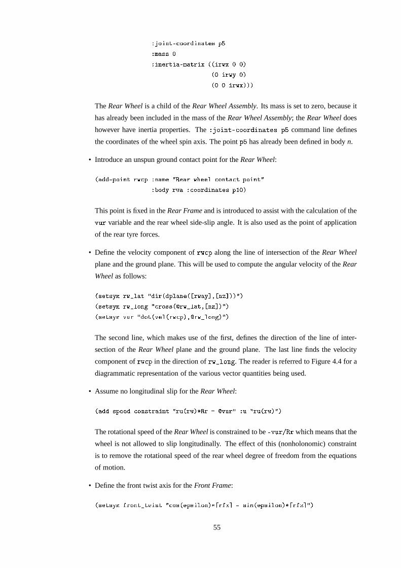
����+��������;�+�+������������� : �� (��������� �.�������'���&(�������� ���.�,�6+�������
��� �,�6�!���������8���6(�������
The Rear Wheel is a child of the Rear Wheel Assembly. Its mass is set to zero, because it
has already been included in the mass of the Rear Wheel Assembly; the Rear Wheel does
however have inertia properties. The � � F � � �>= H F�F �� � � � � � G�� command line defines
the coordinates of the wheel spin axis. The point G�� has already been defined in body n.
• Introduce an unspun ground contact point for the Rear Wheel:
���������.:�+������ �6�;,:#� ���,(��8/������� 6�7����� ;�+5������;'� :�+������I/� *�+���! �6�� ��;�+�+������������� :-4����
This point is fixed in the Rear Frame and is introduced to assist with the calculation of the@� � variable and the rear wheel side-slip angle. It is also used as the point of application
of the rear tyre forces.
• Define the velocity component of � � H G along the line of intersection of the Rear Wheel
plane and the ground plane. This will be used to compute the angular velocity of the Rear
Wheel as follows:
��������,!5( �6�2� ��%/����, ���:� ��5��� � � 6��!�� ��� �(� ������/���������,!5( �6�2� +��� 8/�;,�+����-����6�2� ��"��� �+� ����/����������,!5( ��"�)/���+�� ������ >���6�;,:�� ����6�2� �+'�� ���/��
The second line, which makes use of the first, defines the direction of the line of inter-
section of the Rear Wheel plane and the ground plane. The last line finds the velocity
component of � � H G in the direction of � � � � F � ? . The reader is referred to Figure 4.4 for a
diagrammatic representation of the various vector quantities being used.
• Assume no longitudinal slip for the Rear Wheel:
����������,:���������;�+����,���������� /.�" �#�6I��� ������"�9/ � " /." ���6I��/�
The rotational speed of the Rear Wheel is constrained to be = @ � ������� which means that the
wheel is not allowed to slip longitudinally. The effect of this (nonholonomic) constraint
is to remove the rotational speed of the rear wheel degree of freedom from the equations
of motion.
• Define the front twist axis for the Front Frame:
��������,!5(����+�����2���6I��'� /�;5+��-����:����� �+������ � ������$� ����� ���5:����� �+5�I��� � ��+� �I/5�
55
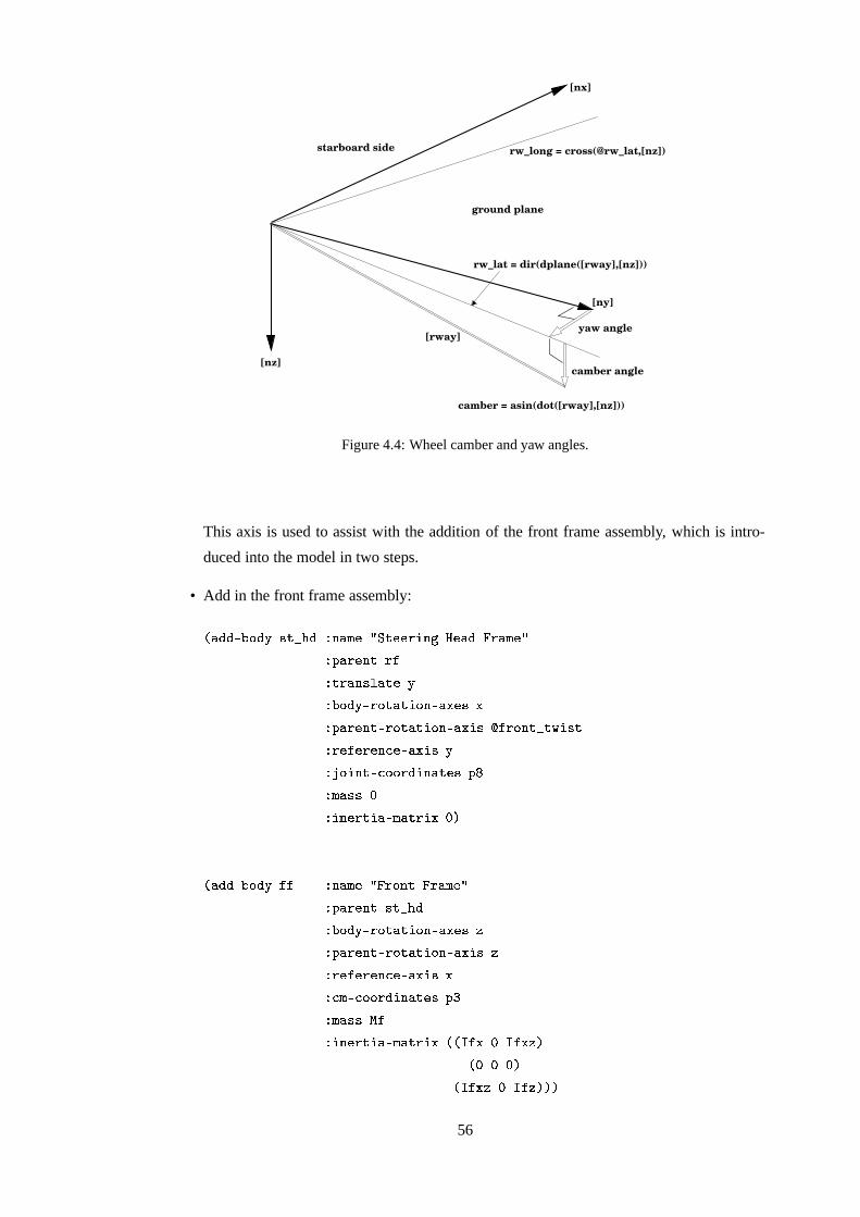
camber = asin(dot([rway],[nz]))
[nx]
ground plane
rw_lat = dir(dplane([rway],[nz]))
[ny]
yaw angle
camber angle
[rway]
[nz]
starboard side rw_long = cross(@rw_lat,[nz])
PSfrag replacements
Figure 4.4: Wheel camber and yaw angles.
This axis is used to assist with the addition of the front frame assembly, which is intro-
duced into the model in two steps.
• Add in the front frame assembly:
���������&����'9%���7+/�� ������� �.���(����� � ����Q�������� ��� ��� � ������ � �#��� ��� � � �#� %(4(�(���6'��&����' � � (���(� �>#�1�+������%������� � �#����� � (���#� �+#�1�������(% : � #����7#��E1��%��� � � � � �+� !#� �+��� ��% '� <� ����� �(!#� � � �����(����%H��J� ����%�%T,�C���� � � �>� � � �(� � ���T, 0
���������&����' ������� �.� ��� +��� ��� ����� ������ � �#��� %���7+/����&����' � � (���(� �>#�1�+������%������ � �#����� � (���#� �+#�1�������(%�� � � � � �+� !#� �+��� ��%���! � ��!#� � �������#����%V��8� ����%�%�� �C���� � � �>� � � �(� � ��� ���� �-,� ����0��,",-, 0
�� ���-,� ��0�0�0
56
To begin, the Steering Head Frame is used to represent lateral displacements and rotational
twist freedoms between the Front Frame and the Rear Frame. The Front Frame is then
added as a child of the Steering Head Frame. The steering freedom, the mass and the
inertia-matrix of the front frame assembly are also included at this point.
• Add in the Front Wheel:
���������.*�+���!$��6 � ���,(�� /����+���� � 7����� �/� :��������$���� *�+��!��,�+������5+����'�������<!� :����������,�+������'+5�I�5������<!� �����������;5���5������������+��.������;�+�+�������������� : �� (��������� ����������5��� (������ � �*�8�'��6�!������
This body has the Front Frame as its parent. Its mass and x and z inertias are zero since
these have been included in the Front Frame description. The spin inertia of the Front
Wheel is included so that angular momentum (gyroscopic) effects are correctly repre-
sented.
• Introduce an unspun ground contact point for the Front Wheel:
���������.:�+������0�6�;,:#� ���,(��8/����+5��� 6�7����� ;�+�������;'� :�+������9/� *�+���! ��� ��;�+�+������������� :94�4�
This point is fixed in the Front Frame. It is introduced to assist with the calculation of the@��
variable and the Front Wheel side-slip angle. It is also used as the point of application
of the front tyre forces.
• Define the velocity component of��H G along the line of intersection of the Front Wheel
plane and the ground plane:
��������,!5(��6�2� ��%/����, ���:� ��5��� � � ���!�� ��� �(� ������/5���������,!5(��6�2� +��� 8/�;,�+����-�����6�2� ��"��� �+� ����/����������,!5( ��"��%/���+�� ������ >���6�;,:�� �����6�2� �+'�� ���/��
The second line, which makes use of the first, defines the direction of the line of inter-
section of the Front Wheel plane and the ground plane. The last line finds the velocity
component of��H G in the direction of
�� � � F � ? .
• No longitudinal slip on the Front Wheel:
����������,:���������;�+����,���������� /.�" ���6I��� ��� ����"��I/ � " /." ���6I��/�
57
As with the Rear Wheel, it is assumed that the Front Wheel undergoes no longitudinal slip.
Consequently, its angular velocity is set to = @ � � ��� � and the rotational speed of the wheel
degree of freedom is eliminated from the equations of motion by AUTOSIM.
• Add in the engine flywheel:
���������.*�+���! ��6 � ���,(��8/����� ������0�� 5!�6�7����� �/� :��������$��� *�+���!��,�+������'+��I�5�������<!� :����������,�+�������5+��I�,������ !� ��������5��;����5���������� (��������� �.�������'���&(�������� �����,�!�����
The Engine Flywheel is a child of the Rear Frame and is located at its origin with freedom
to rotate about the A -axis of the Rear Frame. The Engine Flywheel has a spin inertia
associated with it so that the associated angular momentum effects associated with the
spinning engine can be reproduced in the model.
• The Engine Flywheel is assumed to rotate at the same speed as the Rear Wheel – Its inertia
is adjusted to make this accurate:
����������,:���������;�+����,���������� /.�" �����6I����������"�I/ � " /��" ������6I��/�
The Engine Flywheel rotates with an angular speed of = @ � ����� � and consequently this
freedom is eliminated from the equations of motion.
• Define the camber and side-slip angles:
��������,!5( :�7I�,)/,������� ����+� � � �(� � � � 6�!�������/����������,!5( :�7I�'�%/,������� ����+� � � �(� � � � ��6�!�������/����������,!5( �� 5:�7��%/,�����.� ����+� � ��6�2� ��"� ���� �#���� -��6�;�:I�������/����������,!5( �� 5:�7����8/,�����.� ����+� � ���6�2� ��"� ���� �#���� -����6�;�:I�������/��
These angles are needed in the calculation of the tyre side forces and moments. The first
line defines the Rear Wheel camber angle, the second line defines the Front Wheel camber
angle and the third defines the Rear Wheel side-slip angle by making use of the point � � H Gdefined above. The last line defines the Front Wheel side-slip angle via the point
��H G .
Note that for the side-slip angles, positive lateral velocities give positive slip values and
negative forces.
• Add the driving torque:
�#"��� ������$� ����������
58
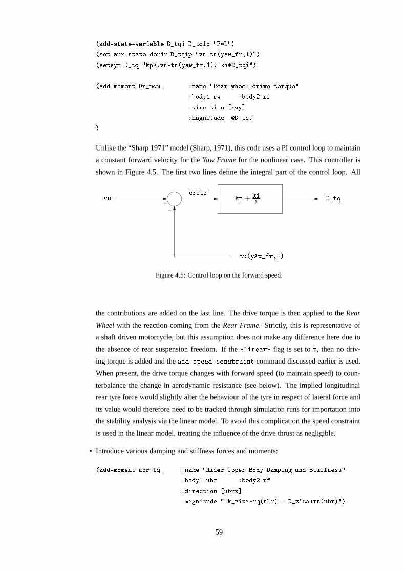
����������'��������,�����'�5*� �� ��25����� ��2�� ����:)/����� �/���������'��"(�����,��������,�����.� ��2������.:)/.��"I�,�" ��!���6�2��"��4���/���������,!5( ��2����%/.1:��-����"��,��" ��!���6�2�� ��4�� 1��� ��2'������/��
��������� (�+,(������ ���2.(�+,( � ����(��8/������ 6�7����� 0����,��� ��+���"���/� *�+��!94 �6 � *�+��! �0��� �������;'���'+�� � 6�!��� (��� ��I�,��"���� � � ��2������
�
Unlike the “Sharp 1971” model (Sharp, 1971), this code uses a PI control loop to maintain
a constant forward velocity for the Yaw Frame for the nonlinear case. This controller is
shown in Figure 4.5. The first two lines define the integral part of the control loop. All
PSfrag replacements ���
� ������� �� ��������
� � ���� �������
+
−
���+� �s
Figure 4.5: Control loop on the forward speed.
the contributions are added on the last line. The drive torque is then applied to the Rear
Wheel with the reaction coming from the Rear Frame. Strictly, this is representative of
a shaft driven motorcycle, but this assumption does not make any difference here due to
the absence of rear suspension freedom. If the �� ���� � � flag is set to � , then no driv-
ing torque is added and the �-= ��G ��� -= H F � ����� � � � command discussed earlier is used.
When present, the drive torque changes with forward speed (to maintain speed) to coun-
terbalance the change in aerodynamic resistance (see below). The implied longitudinal
rear tyre force would slightly alter the behaviour of the tyre in respect of lateral force and
its value would therefore need to be tracked through simulation runs for importation into
the stability analysis via the linear model. To avoid this complication the speed constraint
is used in the linear model, treating the influence of the drive thrust as negligible.
• Introduce various damping and stiffness forces and moments:
��������� (�+,(������ "�*��2���� � ���,(�� /����'������:�:�� ��+���! ����(�:I���� $����� ����'������������/� *�+���!94 "�*� � *�+��! �0��� ���,���;,���5+�� � "�*�+� �� (�� ��I����"���� /�,1�2����,�����' � �#"�*��� � ��2����,�����'" �#"�*����/�
59
��������� (�+,(������0�6���2���� � ���,(�� /������ ��6I���,� ���,(�:I�.�� ����� ����,�����������/� *�+���!94 6�� � *�+��! �0��� ���,���;,���5+�� � �6���� �� (�� ��I����"���� /�,1�2� �,(������,�� ���6���� � ��2� ��,(������'�" ��6�����/��
���������5 ��������,��+�;��0�'��257���2� � ���,(�� /����������.�� ������� �������� �����'������������/� ���,���;,���5+�� ���'��257���!��� :�+������I4 �'��257��+� � :�+������ � �'��257��+�� (�� ��I����"���� /�,1�2����'��� ���,��257���� � ��2����'�" ���'��2'7�����/�
��������� (�+,(������ �'��2'7���2���� � ���,(�� /����+���� ��6����'� ��+���"���/� *�+���!94 �,��257�� � *�+���! �0��� ���,���;,���5+�� ���'��257�� ���� (�� ��I����"���� /�,1�2� ��,(�(����,�� ���'��257���� � ��2� ���(�(����'" ���'��2'7�����/5�
��������� (�+,(������ �'������2���+��� � ���,(�� /����������.�� ����,(�:I���� ����� �����'�����������/� *�+���!94 ��� � *�+��! � �'��2'7��� ���,���;,���5+�� � ���+� �� (�� ��I����"���� /�,1�2��,�������,�� ��������� ��2��'�������'�" ������� ���'��25����/�
All the above moments are generated by torsional springs and dampers except for the
last one which includes an external torque input from the rider – this defaults to zero.
The first one is the moment between the Rider Upper Body and the Rear Frame. The
second is between the Rear Wheel Assembly and the Rear Frame. The third moment is
between the Steering Head Frame and the Rear Frame and the final one is between the
Front Frame and the Steering Head Frame. The �-= � � � � = � F� H�� command introduces
a lateral force between the Steering Head Frame and the Rear Frame via a spring and
damper. Appropriate values for the spring and damper constants are given at the end of
the program listing.
• Introduce the aerodynamic drag and lift forces:
���������.:�+������ :-4���� ���,(�� / '���������$+������������"��� ��� ���/!� *�+���!$�� ��;�+�+���������������<:-4����
���������5 ��������,��+�;������� � ���,(�� / ����+���!���,(>��; ���� I/� ���,���;,���5+�� � �� ���� :�+������I4 :-4��� (�� ��I����"���� /����;��9����" ��!���6�2�� ��4����� ����/�
���������5 ��������,��+�;�� ��,��� � ���,(�� / ����+���!���,(>��; ��'���I/� ���,���;,���5+�� � ��+� �� :�+������I4 :-4��� (�� ��I����"���� /� �;��9����" ��!���6�2�� ��4����� ����/�
The point G E � is used to define the centre of pressure which is a point attached on the
60
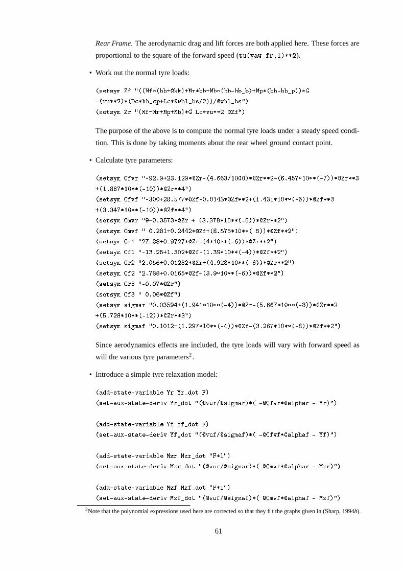
Rear Frame. The aerodynamic drag and lift forces are both applied here. These forces are
proportional to the square of the forward speed ( � ��� A � � � ���,E�� ����� ).
• Work out the normal tyre loads:
��������,!5(����%/�����$����-�#*�*���1�1�� $����*�* $�*��9� *�*I��**�2'*�� $�:��-� *�*I�.*�*�25:������ ��9����"���� �����-� ��;��,7�7�2�;,: �;�� �56�7� 25*�� � ����� � �56�7� �25*���/����������,!5(��)/���$�� $�� $: $�*I������ �;��'��"���� ��� ������/�
The purpose of the above is to compute the normal tyre loads under a steady speed condi-
tion. This is done by taking moments about the rear wheel ground contact point.
• Calculate tyre parameters:
��������,!5( '�����)/� � ���� ������4�� ��� � ����9� ��� � ����4����+���� ������� ���9� ��� ��3���4 ����-���'3������ �������� � �,4 � � � 3���4������-�.��4 ������� �������� 9/5���������,!5( '������%/� �+�+� �� � � ��3�3�� ������ ������4 ��� ��������� � �,4 � ���45��4 ����-��� ������� �������� � � ������3���4������-�.��4 ������� �������� 9/5���������,!5( ''(���)/�� (�������3���� ���� � �����3 � ��4������-�.� ������� � ����� ��/���������,!5( ''(����%/� ��� � � 4 (��� �� ��� � �� � � ����3 ����4������9��� ������ � ������� ��/����������,!5( '�94 /���3 �� � (� ���3 ��3�� ������I� ���4������9�.� ������ � ���� ��/����������,!5( '��I4 /��4���� ��� �4 ��+� ��� ������I�,4 ��������4 �����I�.�������� � ������� ��/���������,!5( '� �8/���� ����� (� ����4�� � ��� � �� � ��� � � ��4������9��� ������� � ������ ��/���������,!5( '����8/���� 3 ��� (� ����4������ ���� � ��������4 �����-�&� ������ ��������� ��/����������,!5( '���8/��� ����3�� � �9/���������,!5( '�� �8/��� ������� � ���I/���������,!5()���, 5(��%/������ ������� �,4 ���I45��4������9���������� � ����9� � �� ��3���4������9��� � ����� � ������ � � ���#3 � � ��4������-�.��4 ������� �����������/5���������,!5()���, 5(����8/�����4 ��4�� ��4 � ����3���4�����-���������� ������I� ��� ����3���4 ����-��� � ����� �������� ��/5�
Since aerodynamics effects are included, the tyre loads will vary with forward speed as
will the various tyre parameters2 .
• Introduce a simple tyre relaxation model:
����������'��������,�����'�5*� �� ������2��+�������������'��"(�����,��������,�����.�%���2��+��%/�� ���"��� ������ 5(�����9� � � '������� ���� ':�7�� � �����/�
����������'��������,�����'�5*� �� ��������2��+�������������'��"(�����,��������,�����.�%����2��+��%/�� ���"���� ������ 5(�������9� � � '�������� ���� ':�7����$� ������/�
����������'��������,�����'�5*� �� $(��$+���2��+��%/���� �/����������'��"(�����,��������,�����.�%$(���2��+�%/�� ��"��� �����, 5(�����-� � ''(����� ���� 5:�7�� � $(�����/��
����������'��������,�����'�5*� �� $(����$+����2��+��%/���� �/����������'��"(�����,��������,�����.�%$(����2��+�%/�� ��"���� �����, 5(�������-� � ''(������ ���� 5:�7���� � $(������/��
2Note that the polynomial expressions used here are corrected so that they fit the graphs given in (Sharp, 1994b).
61
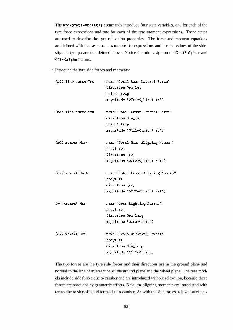
The �-= ��� � � = @ � � B ��� commands introduce four state variables, one for each of the
tyre force expressions and one for each of the tyre moment expressions. These states
are used to describe the tyre relaxation properties. The force and moment equations
are defined with the � � � = � � = ��� � � = � � �@ expressions and use the values of the side-
slip and tyre parameters defined above. Notice the minus sign on the � � E ��� �� G�� � and
� � E ��� �� G�� � terms.
• Introduce the tyre side forces and moments:
���������5 ��������,��+�;�� ���� � ���,(�� / ��+���� ������ �������� ���+�;5��/� ���,���;,���5+�� ��6�2� ��� :�+������I4 �6�;,:� (�� ��I����"���� / � '�945� ��:�7I�����9/�
���������5 ��������,��+�;�� ���� � ���,(�� / ��+���� ����+���� ��������� ���+�;���/� ���,���;,���5+�� ���6�2� ��� :�+������I4 �6�;,:� (�� ��I����"���� / � '��I45� ��:�7I�,� ����I/�
��������� (�+,(�������$(���� � ���,(�� / ��+���� ������ �� ��, ������� �$�+,(������9/� *�+���!94 6��� ���,���;,���5+�� � � � �� (�� ��I����"���� / � '� ��� ��:�7I���$(��9/�
��������� (�+,(�������$(���� � ���,(�� / ��+���� ����+���� �� ��, �I���� $�+,(������I/� *�+���!94 ���� ���,���;,���5+�� � � � �� (�� ��I����"���� / � '������ ��:�7I�,� �$(���I/�
��������� (�+,(�������$+�� � ���,(�� /����������, �7������� $�+,(������I/� *�+���!94 6��� ���,���;,���5+�� ��6�2� +��� � (�� ��I����"���� / � '����� ��:�7I��9/�
��������� (�+,(�������$+��� � ���,(�� /����+��������� �7������� �$�+,(������9/� *�+���!94 ���� ���,���;,���5+�� ���6�2� +��� � (�� ��I����"���� / � '�� ��� ��:�7I�,�I/�
The two forces are the tyre side forces and their directions are in the ground plane and
normal to the line of intersection of the ground plane and the wheel plane. The tyre mod-
els include side forces due to camber and are introduced without relaxation, because these
forces are produced by geometric effects. Next, the aligning moments are introduced with
terms due to side-slip and terms due to camber. As with the side forces, relaxation effects
62
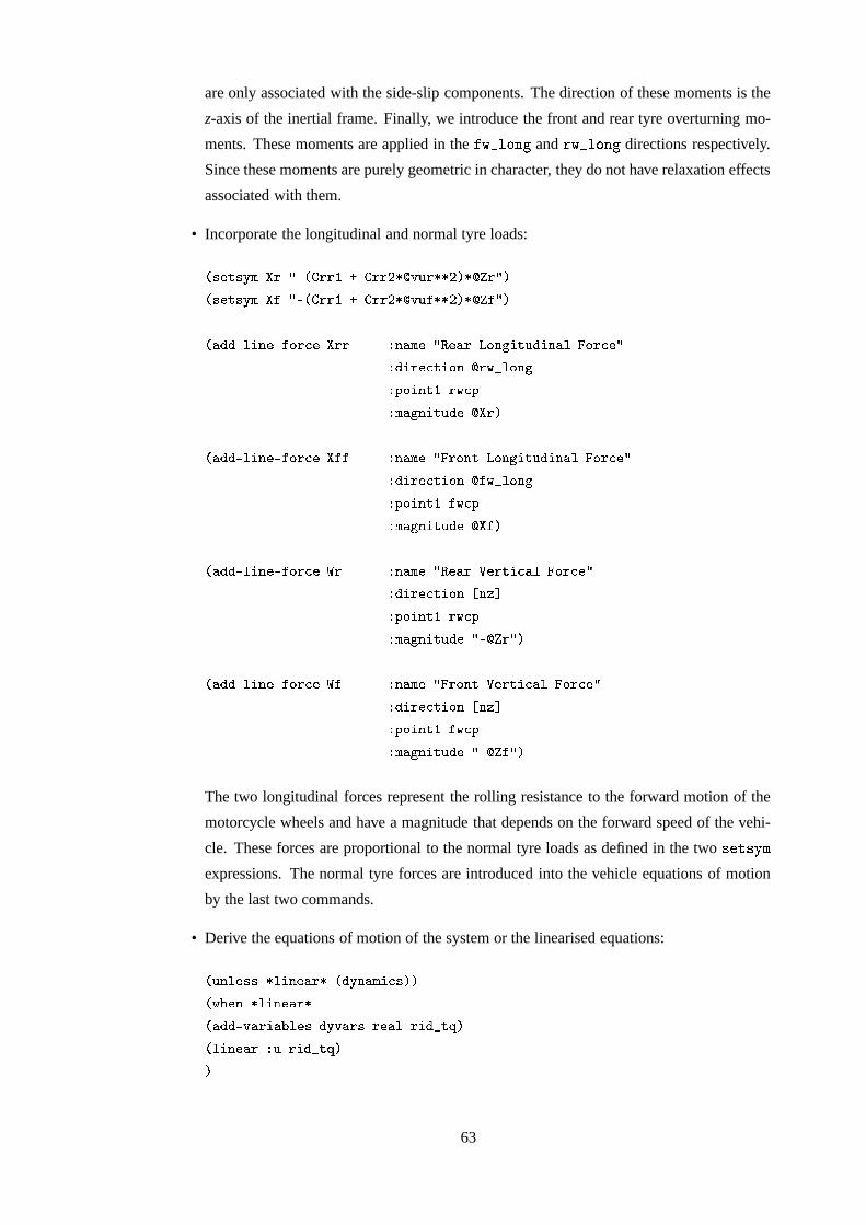
are only associated with the side-slip components. The direction of these moments is the
z-axis of the inertial frame. Finally, we introduce the front and rear tyre overturning mo-
ments. These moments are applied in the�� � � F � ? and � � � � F � ? directions respectively.
Since these moments are purely geometric in character, they do not have relaxation effects
associated with them.
• Incorporate the longitudinal and normal tyre loads:
��������,!5(���)/�9�*'�94 �'�� ��� ���"����� ����� � ��9/���������,!5(����%/�9�*'�94 �'�� ��� ���"������ ����� � ��I/�
���������5 ��������,��+�;�� ��� � ���,(�� /������ �+��� ��,��"����.���� ��+�;���/� ���,���;,���5+�� ��6�2� +��� � :�+������I4 �6�;,:� (�� ��I����"���� ������
���������5 ��������,��+�;�� ����� � ���,(�� /����+���� �+5�� ��,��"��������� ��+�;5��/� ���,���;,���5+�� ���6�2� +��� � :�+������I4 �6�;,:� (�� ��I����"���� �������
���������5 ��������,��+�;�� � � ���,(�� /������ � ������;��� ��+�;���/� ���,���;,���5+�� � � � �� :�+������I4 �6�;,:� (�� ��I����"���� /� ���I/�
���������5 ��������,��+�;�� � � � ���,(�� /����+���� � �������;��� ���+�;���/� ���,���;,���5+�� � � � �� :�+������I4 �6�;,:� (�� ��I����"���� /� ������/�
The two longitudinal forces represent the rolling resistance to the forward motion of the
motorcycle wheels and have a magnitude that depends on the forward speed of the vehi-
cle. These forces are proportional to the normal tyre loads as defined in the two � � � �A �expressions. The normal tyre forces are introduced into the vehicle equations of motion
by the last two commands.
• Derive the equations of motion of the system or the linearised equations:
�#"��� ������$� ����������%����!����,(-��;�������#6�7����8� �������������������������5�5*� ���� ��!������� ����� 0��,��2������� ���������� " ��'��25������
63
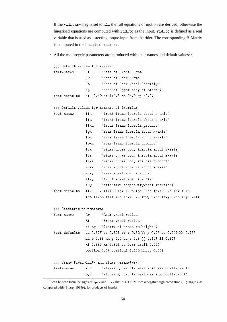
If the �� ���� � � flag is set to �
� �the full equations of motion are derived; otherwise the
linearised equations are computed with � � � � � as the input. � � � � � is defined as a real
variable that is used as a steering torque input from the rider. The corresponding B-Matrix
is computed in the linearised equations.
• All the motorcycle parameters are introduced with their names and default values3:
����� �������5"� ��$���� '"���� ��+ (���������� ���������.���,(���� $�� / $������ +������+5��������,(���/
$� / $������ +��������������,(���/$�* / $������ +��������� � 7����� �������,(�*� 5!9/$�: / $������ +�����:�:�� ��+���! +������'���9/�
��������,��������"� ���� $�� ������� $�)4,3+���� $�* ��� ��� $�: � �������
����� �������5"� ��$���� '"���� ��+ (�+�(�������� +�%���������5� ���������.���,(���� &'��� /.���+���� ���,(�� ���������5�$�5*�+�"������5��������/
&'� � /.���+���� ���,(�� ���������5�$�5*�+�"������5��������/&'���(� /.���+���� ���,(�� ���������5� :��+��"�;,�9/&�:+� /����� ����,(������������5� ��*�+�"������5��������/&�:(� /����� ����,(������������5� ��*�+�"������5��������/&�:+�(� /����� ����,(������������5� :��+��"�;'�I/&, � /���'��� "�:�:�� *�+��!8���������5�$��*�+�"������5�������/&,+� /���'��� "�:�:�� *�+��!8���������5�$��*�+�"������5�������/&, �(� /���'��� "�:�:�� *�+��!8���������5� :��+���"�;'�9/�,6(� /����� 6�7����� ���������5� ��*�+�"������5��������/�,6�! /����� 6�7����� �,:I���%���������5��/�'��6�! /.���+���� 6�7����� �,:����%���������5��/�,�! /���������;,���,��� ���� ������ �� �!�6�7����� ����������5��/��
��������,��������"� ���� &'��� ��� ��3 &'� �(���,&�:(�)4 ���� &�:(��� � ��� &�:(�(����� ��� &,+� 3�����&,+� 4�4 ����&,+�+� 3 ��8�,�6(������8�,6�!���������'�6�!� � � � �,�!�����I4�
����� ����+,(�������; :����,(������� ���������.���,(���� �� / ����� 6�7����� 0������."���/
��� / ���+���� 6�7����� ������"���/7�7�2�;,: /�'���������$+�� :��������"��� 7����, �7��9/��
��������,��������"� ���� ������� � ��30*�*���� � � *�*�25*���� � *�*�25:��� � � ���������� � 7�7)� ���� �7�7�25*������07�7�2': � ��$7�7�2������ � �+����� � ��3 � ���� � ��3�������� ��� ������� ��40������� 3�3 ������� ���� ������:����� �+���� ���3 ��:����5 �+��-4 4 ������ 7�7�2�;,:��������
����� ����,(�� �� �������*��� ��,��! �����$��'���$:����,(������� ���������.���,(���� 1�25� /5�'���������� 07������ �������� �'���,��������0;�+���������;��5�����9/
��25� /5�'���������� 07������ �������� ���,(�:I���� �;�+���������;��5�����9/3It can be seen from the signs of ��� ��� and � ����� that AUTOSIM uses a negative sign convention (−∑mixizi), as
compared with (Sharp, 1994b), for products of inertia.
64

1�2� ��,(���� /����� 6�7����� $��������(�*� �! �6I���'� �'���,����������0;�+��������;��'�����9/��2� ��,(���� /����� 6�7����� $��������(�*� �! �6I���'� ���,(�:I���� ;5+��������;��5�����I/1�25 ��,(�(�� /5�'���������� 07������$��+����'+����� �'���'����������� ;5+��������;��5�����I/��25 ��,(�(�� /5�'���������� 07������$��+����'+����� ���,(�:I�.�� �;�+���������;��5�5���9/1�2����,��� /���'��� "�:�:�� *�+��! ����'���������� �,���'���������� ;�+���������;��5�����9/��2����,��� /���'��� "�:�:�� *�+��! ����'����������$���,(�:I���� �;�+���������;��5�����9/1�2��'�����%/5�'�������,���'���������� ;�+���������;��5�����9/��2��'�����%/5�'����� ���,(�:I���� �;�+���������;��5�����9/�
��������,��������"� ���� 1�25� /�4 ������-��4�����������/ ��2�� ��� 1�2� ���(���� ��+� �+� ��2� ���(���� 4,3�� 31�25 ��,(�(�� ��4��+�+� ��25 ��,(�(�� ���4 1�2�������� 4��+�+� � ��2����,��� 4������
�#"��� ������$�,7����������5+����8���������'��������"� �����&'�+����� 3�4 1�2��'��������������2��,�����%4 � ������#6�7����8�,7����������'+����8�&������'��������"� 5����&,�+�������4 1�2��,����� �+� ������2��'����� ���������
����� ��!���0:�����,(������� ���������.���,(���� � '������ / ���+���� ��!����'�+��������� ����'������������/
� '����� / ����� ��!����'�+���������� �����'�����������/� ',(���� / ���+���� ��!������ ��, �I���� $�+,(������ �����'�����������/� ',(��� / ����� ��!������ ��, ������� $�+�(������ ����,�����������/� '��I4 / ���+���� ��!����'��,(�*�� ����'�����������/� '94 / ����� ��!����'��,(�*��� ����'������������/� '���� / ���+���� ��!������ ��, �I���� $�+,(�������'��,(�*���'�+��������;��5�����I/� ' � / ����� ��!������ ��, ������� $�+�(�������'��,(�*���'�+��������;��'�����9/� '�� � / ���+���� ��!��� ��������"���I�.�� �$�+�(�������'�+���������;��5�����9/� '�� / ����� ��!��� �������"���I���� �$�+,(�������'�+��������;��'�����9/'��94 / ��!���0�+� � ����� $��������'������;��$;�+���������;��5����� 4�/'�� � / ��!���0�+� � ����� $��������'������;��$;�+���������;��5����� ��/�
��������,��������"� ���� '��94%������4 � '�� �8/���� � ��4������-��� ����/�
����� ����7��� :����,(�������� ���������.���,(���� ��; / ����+��!����,(>�; ���� �'�+���������;��5�����9/
�; / ����+��!����,(>�; ��,����'�+���������;��5�����9/���������,��������"� ���� ��; �����3�3 �;�������� ��" ����� ����#"��� ������$� ����������%�&������'��������"� 5��� �,����:�����+��4 �'��+�:�� �+� ��:�������%4�� ��'��2������
1�� �+�+� 1�: �+�+�8/.�" ��!���6�2��"��4���/ �" /. � �������/ �����+� �����
The � � � ��=�F � � flag is used to choose the appropriate values for the parameters corre-
sponding to the hands-off and hands-on cases. Strictly speaking, for the hands-on case, the
reaction to the steering restraint torque ( � � ��� � � � � ) comes from both the Steering Head
( � � �� ) and the Rider Upper Body ( � B�� ) and not only from the Steering Head as in the
hands-off case, but this is neglected. The last line sets some default values relevant only
to the nonlinear model.
• Write up files:
65
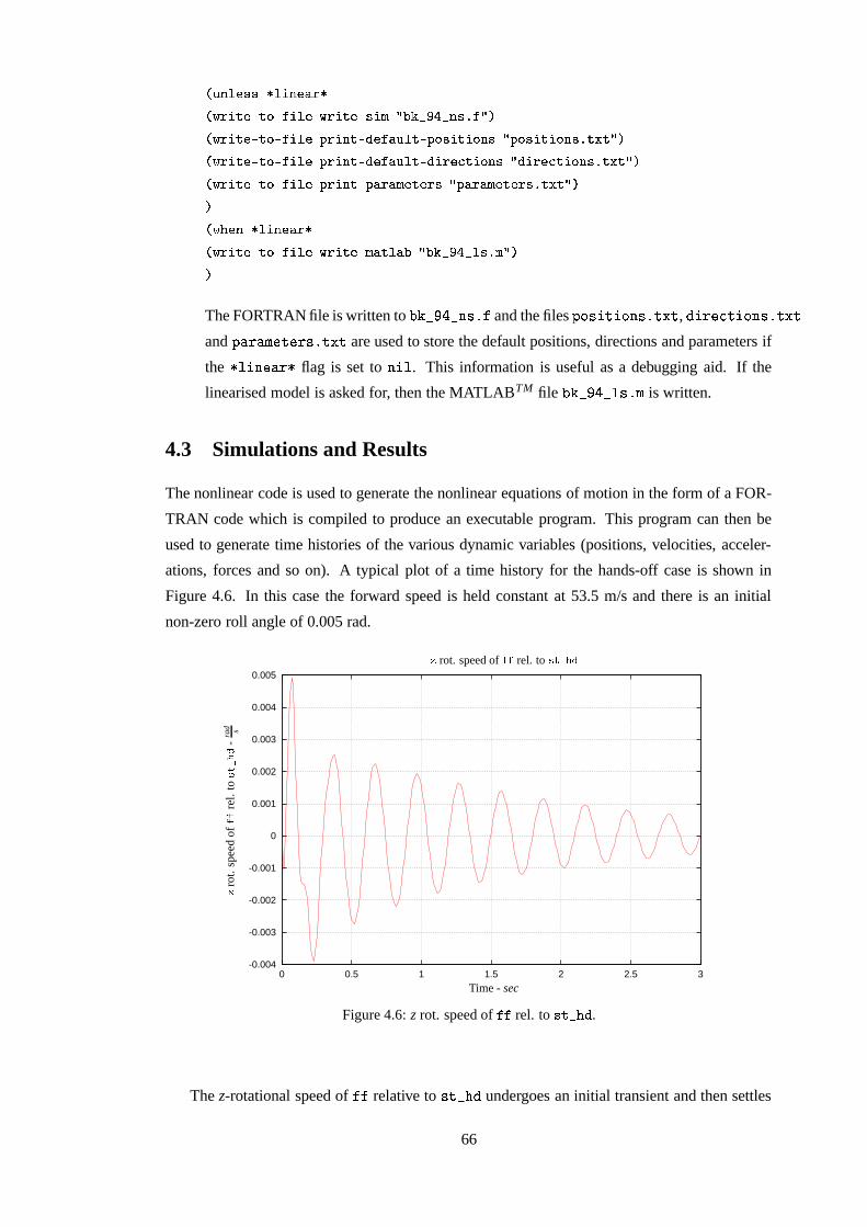
�#"��� ������$� �����������#6���,�����,��+��,���� �� 6���,���������&( /�*�1�2 ���25��� � �I/��#6���,�����,��+��,���� �� :���������'��������"� ����.:�+����.���'+5��� /�:�+��������5+���� � �+���9/5��#6���,�����,��+��,���� �� :���������'��������"� ����,���,���;'���'+5���0/��������;'���'+���� � � ���9/���#6���,�����,��+��,���� �� :����������:����,(�������� /�:�����(������� � �+����/���#6�7����8� �����������#6���,�����,��+��,���� �� 6���,�����&(���� ���*�/�*�1�2 ���2� �� � ( /��
The FORTRAN file is written to B�C ����� � � ��� � and the files G�F � � � � F � ��� � � � , � � ��H � � F � �� � � �and G � �� � � � � ��� � � � are used to store the default positions, directions and parameters if
the �� ���� � � flag is set to �
� �. This information is useful as a debugging aid. If the
linearised model is asked for, then the MATLABTM file B�C ����� � � ��� � is written.
4.3 Simulations and Results
The nonlinear code is used to generate the nonlinear equations of motion in the form of a FOR-
TRAN code which is compiled to produce an executable program. This program can then be
used to generate time histories of the various dynamic variables (positions, velocities, acceler-
ations, forces and so on). A typical plot of a time history for the hands-off case is shown in
Figure 4.6. In this case the forward speed is held constant at 53.5 m/s and there is an initial
non-zero roll angle of 0.005 rad.
-0.004
-0.003
-0.002
-0.001
0
0.001
0.002
0.003
0.004
0.005
0 0.5 1 1.5 2 2.5 3
PS
fragreplacem
ents
� rot. speed of���
rel. to �������
� rot
.spe
edof
rel.
to
������
-ra
d s
Time - sec
Figure 4.6: z rot. speed of���
rel. to�,��257��
.
The z-rotational speed of� �
relative to ������� undergoes an initial transient and then settles
66
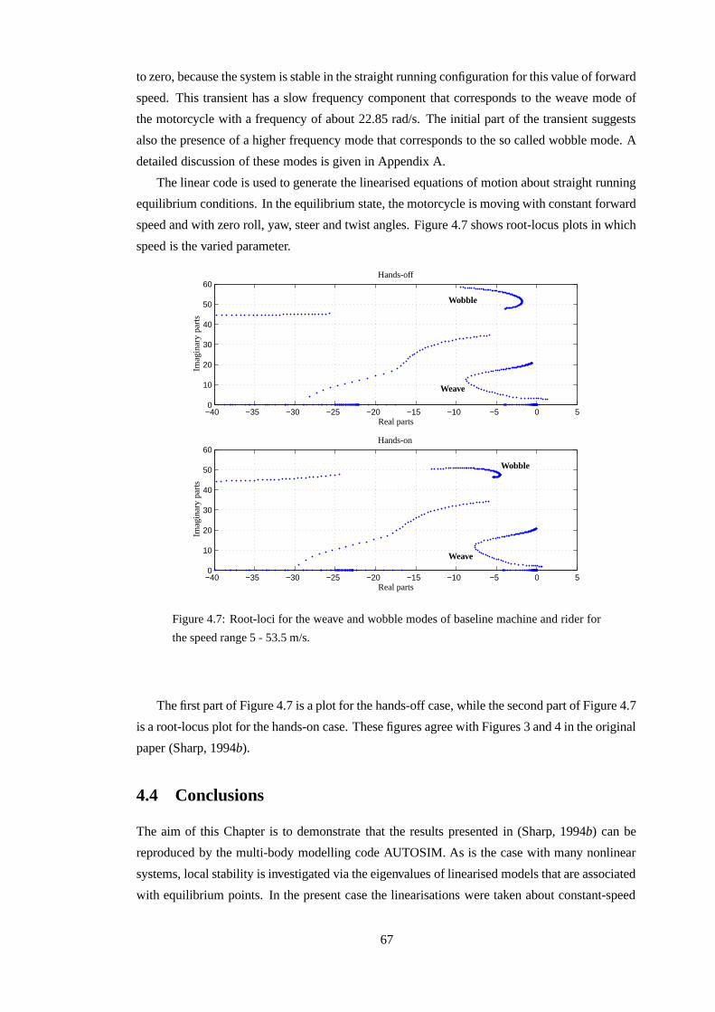
to zero, because the system is stable in the straight running configuration for this value of forward
speed. This transient has a slow frequency component that corresponds to the weave mode of
the motorcycle with a frequency of about 22.85 rad/s. The initial part of the transient suggests
also the presence of a higher frequency mode that corresponds to the so called wobble mode. A
detailed discussion of these modes is given in Appendix A.
The linear code is used to generate the linearised equations of motion about straight running
equilibrium conditions. In the equilibrium state, the motorcycle is moving with constant forward
speed and with zero roll, yaw, steer and twist angles. Figure 4.7 shows root-locus plots in which
speed is the varied parameter.
−40 −35 −30 −25 −20 −15 −10 −5 0 50
10
20
30
40
50
60
−40 −35 −30 −25 −20 −15 −10 −5 0 50
10
20
30
40
50
60
PSfrag replacements
Hands-on
Real parts
Real parts
Imag
inar
ypa
rts
Imag
inar
ypa
rts
Hands-off
Wobble
Wobble
Weave
Weave
Figure 4.7: Root-loci for the weave and wobble modes of baseline machine and rider for
the speed range 5 - 53.5 m/s.
The first part of Figure 4.7 is a plot for the hands-off case, while the second part of Figure 4.7
is a root-locus plot for the hands-on case. These figures agree with Figures 3 and 4 in the original
paper (Sharp, 1994b).
4.4 Conclusions
The aim of this Chapter is to demonstrate that the results presented in (Sharp, 1994b) can be
reproduced by the multi-body modelling code AUTOSIM. As is the case with many nonlinear
systems, local stability is investigated via the eigenvalues of linearised models that are associated
with equilibrium points. In the present case the linearisations were taken about constant-speed
67
straight running conditions. AUTOSIM can be used to generate time histories from the nonlinear
equations of motion, and most usefully, it can be used to generate linearised state-space models
in symbolic form. The linearised models can be imported into MATLABTM for evaluation. A
typical local stability study will require time histories from the nonlinear model and the symbolic
linearised equations of motion generated by the linear AUTOSIM code. The nonlinear equations
are stored in the FORTRAN file B�C ����� � � ��� � and the linearised equations of motion are stored
in the MATLABTM file B�C������ � � �� � . In order to construct the root-loci in Figure 4.7, two lines
have to be removed from this code: the first line which is aH����� � statement and second a line
containing the � ����� � � � statement. The modified version of the MATLABTM file is stored in
B�C������ � � �� � and the diagrams in Figure 4.7 may be generated using this file and the hand-
written plotting code B�C������ ��IF�F � � F H � �� � .
68
Chapter 5
The “SL2001” motorcycle model
5.1 The Mathematical Model
The basic components of the vehicle are:
(a) separate bodies for the front and rear frame that are joined by an inclined steering axis;
(b) a rear frame that is allowed longitudinal, lateral and heave translational freedoms, as well
as yaw, pitch and roll angular freedoms;
(c) a swinging arm and its associated rear suspension system;
(d) telescopic front forks and the associated front suspension system;
(e) spinning road wheels;
(f) twist and steer freedoms for the rear frame relative to the front frame;
(g) longitudinal tyre forces proportional to and opposed to the longitudinal slip as defined in
(Pacejka and Sharp, 1991)1;
(h) lateral tyre forces and moments decoupled from the longitudinal tyre forces, and computed
using the empirical expressions given in (Koenen, 1983);
(i) first order lags to represent tyre relaxation effects, whereby the tyre forces and moments
do not respond immediately to changes in the tyre slip (dynamic tyres)2;
(j) overturning moments due to camber assumed to be instantaneous functions of the tyre
contact geometry (Sharp and Limebeer, 2001; Sharp et al., 1999).
1Checks are made to ensure that these longitudinal tyre forces do not exceed 80% of the normal tyre load. If this
figure is exceeded by either tyre at any point during a simulation run the results are deemed invalid, because they lie
outside the tyre model’s intended operating regime.2Relaxation effects are associated with the lateral force systems, but not with the longitudinal ones. The wheel
aligning moments due to side-slip include relaxation effects, while those due to camber are assumed instantaneous.
69
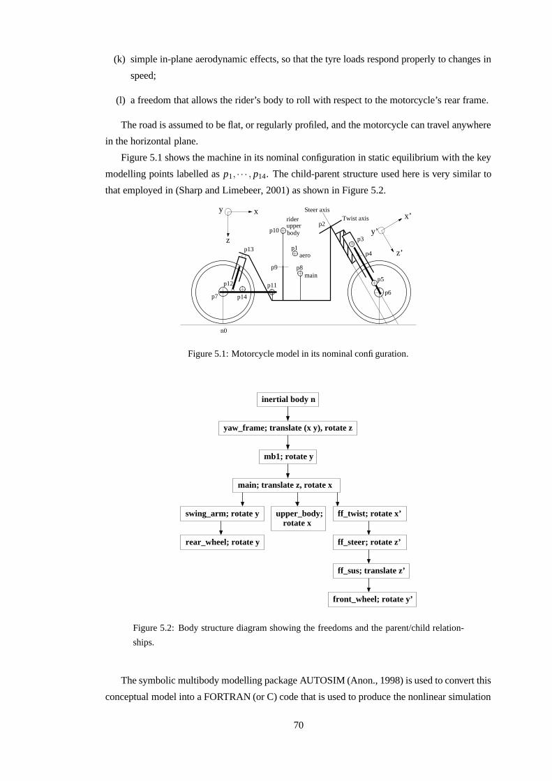
(k) simple in-plane aerodynamic effects, so that the tyre loads respond properly to changes in
speed;
(l) a freedom that allows the rider’s body to roll with respect to the motorcycle’s rear frame.
The road is assumed to be flat, or regularly profiled, and the motorcycle can travel anywhere
in the horizontal plane.
Figure 5.1 shows the machine in its nominal configuration in static equilibrium with the key
modelling points labelled as p1, · · · , p14. The child-parent structure used here is very similar to
that employed in (Sharp and Limebeer, 2001) as shown in Figure 5.2.
zp1
p2
p3
p4
p5
p6p7
p8
p10
p11p12
p13
p14
p9
Steer axisTwist axis
aero
main
riderupperbody
n0
x’
y’
z’
xy
Figure 5.1: Motorcycle model in its nominal configuration.
rear_wheel; rotate y
inertial body n
yaw_frame; translate (x y), rotate z
mb1; rotate y
main; translate z, rotate x
swing_arm; rotate y upper_body;rotate x
ff_twist; rotate x’
ff_steer; rotate z’
ff_sus; translate z’
front_wheel; rotate y’
Figure 5.2: Body structure diagram showing the freedoms and the parent/child relation-
ships.
The symbolic multibody modelling package AUTOSIM (Anon., 1998) is used to convert this
conceptual model into a FORTRAN (or C) code that is used to produce the nonlinear simulation
70
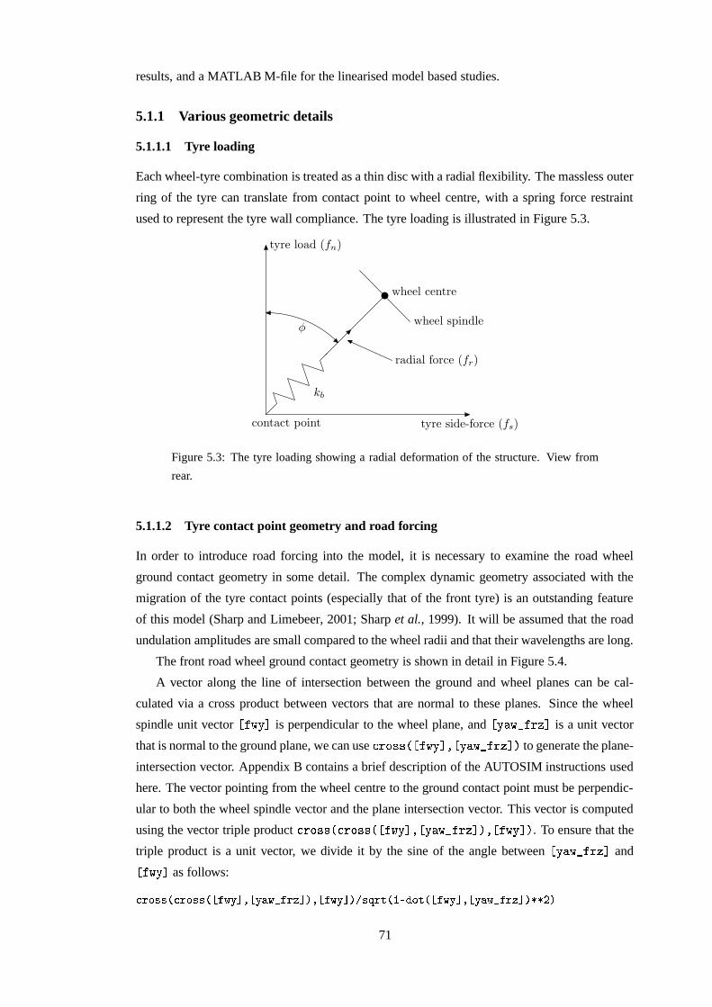
results, and a MATLAB M-file for the linearised model based studies.
5.1.1 Various geometric details
5.1.1.1 Tyre loading
Each wheel-tyre combination is treated as a thin disc with a radial flexibility. The massless outer
ring of the tyre can translate from contact point to wheel centre, with a spring force restraint
used to represent the tyre wall compliance. The tyre loading is illustrated in Figure 5.3.
contact point tyre side-force (fs)
tyre load (fn)
φ
wheel centre
wheel spindle
radial force (fr)
kb
Figure 5.3: The tyre loading showing a radial deformation of the structure. View from
rear.
5.1.1.2 Tyre contact point geometry and road forcing
In order to introduce road forcing into the model, it is necessary to examine the road wheel
ground contact geometry in some detail. The complex dynamic geometry associated with the
migration of the tyre contact points (especially that of the front tyre) is an outstanding feature
of this model (Sharp and Limebeer, 2001; Sharp et al., 1999). It will be assumed that the road
undulation amplitudes are small compared to the wheel radii and that their wavelengths are long.
The front road wheel ground contact geometry is shown in detail in Figure 5.4.
A vector along the line of intersection between the ground and wheel planes can be cal-
culated via a cross product between vectors that are normal to these planes. Since the wheel
spindle unit vector� �� A�� is perpendicular to the wheel plane, and
� A � � � ����� is a unit vector
that is normal to the ground plane, we can useH �IF � � � � � � A�� � � A � � � ����� � to generate the plane-
intersection vector. Appendix B contains a brief description of the AUTOSIM instructions used
here. The vector pointing from the wheel centre to the ground contact point must be perpendic-
ular to both the wheel spindle vector and the plane intersection vector. This vector is computed
using the vector triple productH ��F � � � H �IF ��� � � � � A�� � � A � � � ����� � � � � � A�� � . To ensure that the
triple product is a unit vector, we divide it by the sine of the angle between� A � � � ����� and
� �� A�� as follows:
;'�+����-��;'�+����-� � �6�! � � � !���6�2��+� ��� ��� ��6�!���� ��� ��� �.4�'��+�� � � �56�! � � � !��'6�2��+� ������� ���
71
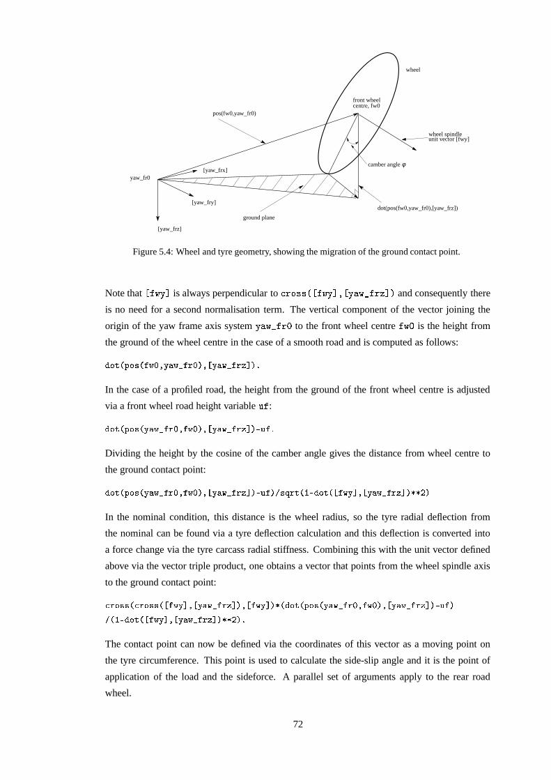
PSfrag replacements
pos(fw0,yaw_fr0)
front wheelcentre, fw0
wheel
horizontal
camber angle φ
projection of
wheel spindleunit vector [fwy]
dot(pos(fw0,yaw_fr0),[yaw_frz])
ground plane
fw_latfw_long
[yaw_frx]
[yaw_fry]
[yaw_frz]
yaw_fr0
Figure 5.4: Wheel and tyre geometry, showing the migration of the ground contact point.
Note that� �� A�� is always perpendicular to
H �IF � � � � � � A�� � � A � � � ����� � and consequently there
is no need for a second normalisation term. The vertical component of the vector joining the
origin of the yaw frame axis system A � � � ��� to the front wheel centre�� � is the height from
the ground of the wheel centre in the case of a smooth road and is computed as follows:
��+� �#:�+��-���6 � �#!���6�2��(��� ��� !��56�2��(� ��� �
In the case of a profiled road, the height from the ground of the front wheel centre is adjusted
via a front wheel road height variable ��:
��+� �#:�+��-�#!���6�2� � �#��6 ��� ��� !��56�2��(� �����."�� �
Dividing the height by the cosine of the camber angle gives the distance from wheel centre to
the ground contact point:
��+� �#:�+��-�#!���6�2� � �#��6 ��� ��� !��56�2��(� �����."���� ��� ��� �.4�'��+�� � � �56�! � � � !��'6�2��+� ������� ���
In the nominal condition, this distance is the wheel radius, so the tyre radial deflection from
the nominal can be found via a tyre deflection calculation and this deflection is converted into
a force change via the tyre carcass radial stiffness. Combining this with the unit vector defined
above via the vector triple product, one obtains a vector that points from the wheel spindle axis
to the ground contact point:
;'�+����-��;'�+����-� � �6�! � � � !���6�2��+� ��� ��� ��6�!������-����+�� � :�+��9�#!���6�25��(� �#�6 ��� � � !���6�25��+� ������"����� �,4��'��+� ��� �6�!�� ��� !��56�2��(� ������ ��� �
The contact point can now be defined via the coordinates of this vector as a moving point on
the tyre circumference. This point is used to calculate the side-slip angle and it is the point of
application of the load and the sideforce. A parallel set of arguments apply to the rear road
wheel.
72
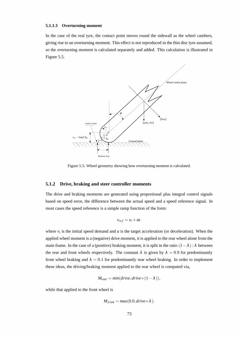
5.1.1.3 Overturning moment
In the case of the real tyre, the contact point moves round the sidewall as the wheel cambers,
giving rise to an overturning moment. This effect is not reproduced in the thin disc tyre assumed,
so the overturning moment is calculated separately and added. This calculation is illustrated in
Figure 5.5.
Wheel centre plane
Moment Arm
Ground plane
contact centre
PSfrag replacementsrtc − load/kb kb
φ
rtc
[yaw_frz][fwy]
Figure 5.5: Wheel geometry showing how overturning moment is calculated.
5.1.2 Drive, braking and steer controller moments
The drive and braking moments are generated using proportional plus integral control signals
based on speed error, the difference between the actual speed and a speed reference signal. In
most cases the speed reference is a simple ramp function of the form:
vre f = vi +at.
where vi is the initial speed demand and a is the target acceleration (or deceleration). When the
applied wheel moment is a (negative) drive moment, it is applied to the rear wheel alone from the
main frame. In the case of a (positive) braking moment, it is split in the ratio (1−λ ) : λ between
the rear and front wheels respectively. The constant λ is given by λ = 0.9 for predominantly
front wheel braking and λ = 0.1 for predominantly rear wheel braking. In order to implement
these ideas, the driving/braking moment applied to the rear wheel is computed via,
Mrear = min(drive,drive∗ (1−λ )),
while that applied to the front wheel is
M f ront = max(0.0,drive∗λ ).
73
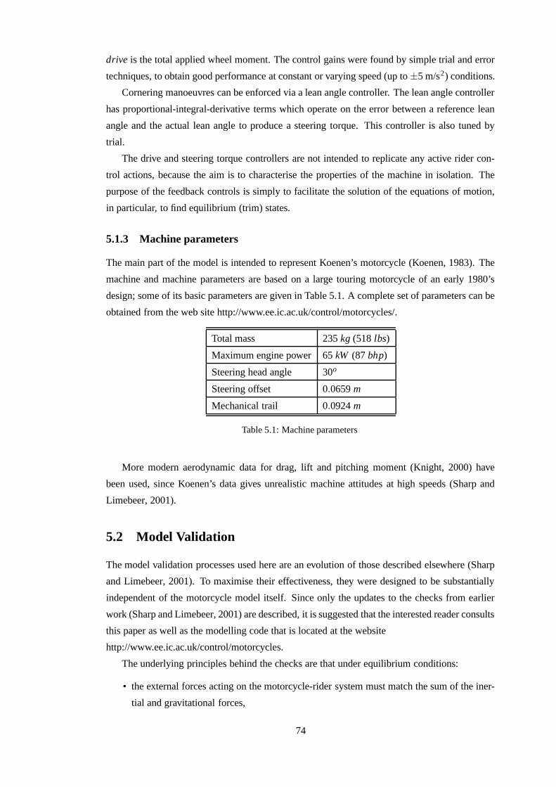
drive is the total applied wheel moment. The control gains were found by simple trial and error
techniques, to obtain good performance at constant or varying speed (up to ±5 m/s2) conditions.
Cornering manoeuvres can be enforced via a lean angle controller. The lean angle controller
has proportional-integral-derivative terms which operate on the error between a reference lean
angle and the actual lean angle to produce a steering torque. This controller is also tuned by
trial.
The drive and steering torque controllers are not intended to replicate any active rider con-
trol actions, because the aim is to characterise the properties of the machine in isolation. The
purpose of the feedback controls is simply to facilitate the solution of the equations of motion,
in particular, to find equilibrium (trim) states.
5.1.3 Machine parameters
The main part of the model is intended to represent Koenen’s motorcycle (Koenen, 1983). The
machine and machine parameters are based on a large touring motorcycle of an early 1980’s
design; some of its basic parameters are given in Table 5.1. A complete set of parameters can be
obtained from the web site http://www.ee.ic.ac.uk/control/motorcycles/.
Total mass 235 kg (518 lbs)
Maximum engine power 65 kW (87 bhp)
Steering head angle 30o
Steering offset 0.0659 m
Mechanical trail 0.0924 m
Table 5.1: Machine parameters
More modern aerodynamic data for drag, lift and pitching moment (Knight, 2000) have
been used, since Koenen’s data gives unrealistic machine attitudes at high speeds (Sharp and
Limebeer, 2001).
5.2 Model Validation
The model validation processes used here are an evolution of those described elsewhere (Sharp
and Limebeer, 2001). To maximise their effectiveness, they were designed to be substantially
independent of the motorcycle model itself. Since only the updates to the checks from earlier
work (Sharp and Limebeer, 2001) are described, it is suggested that the interested reader consults
this paper as well as the modelling code that is located at the website
http://www.ee.ic.ac.uk/control/motorcycles.
The underlying principles behind the checks are that under equilibrium conditions:
• the external forces acting on the motorcycle-rider system must match the sum of the iner-
tial and gravitational forces,
74
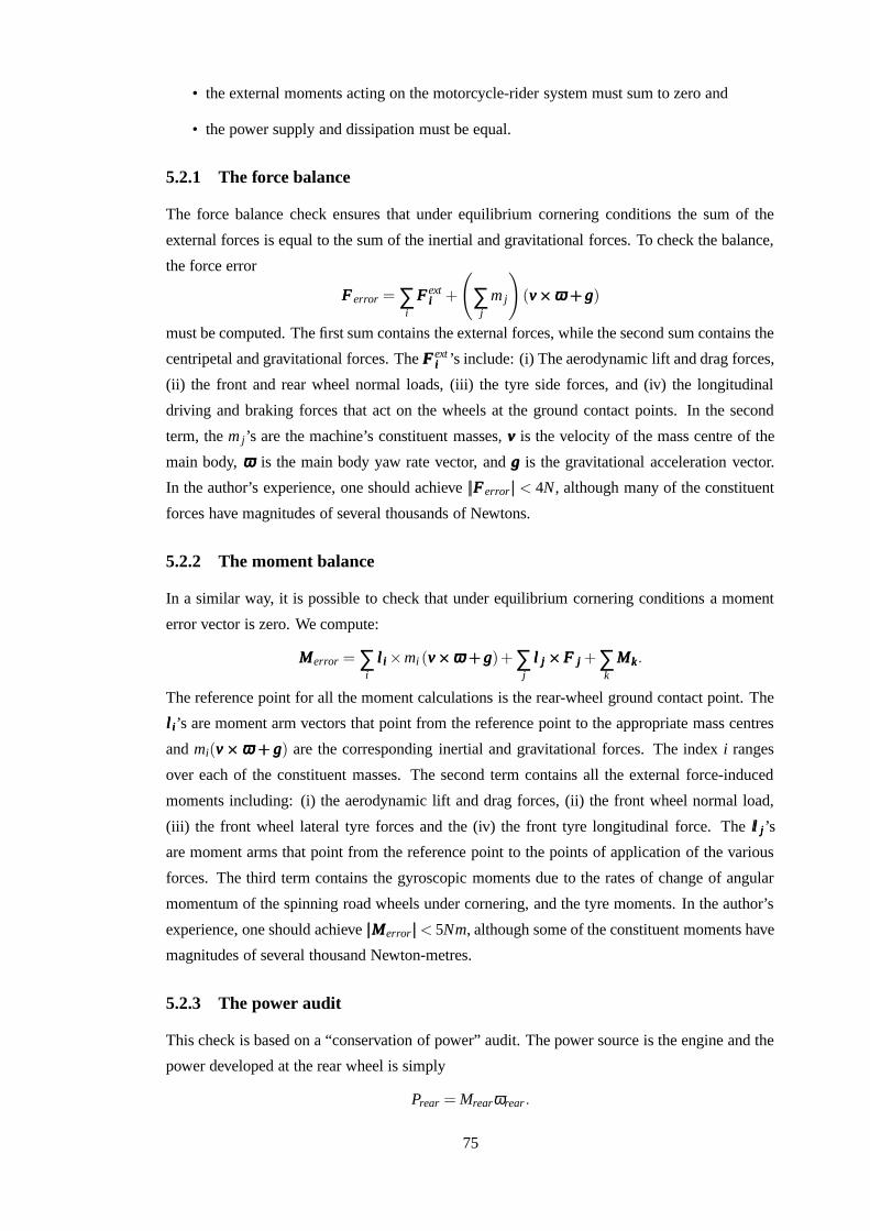
• the external moments acting on the motorcycle-rider system must sum to zero and
• the power supply and dissipation must be equal.
5.2.1 The force balance
The force balance check ensures that under equilibrium cornering conditions the sum of the
external forces is equal to the sum of the inertial and gravitational forces. To check the balance,
the force error
FFFerror = ∑i
FFFextiii +
(
∑j
m j
)
(vvv×××ωωω +++ggg)
must be computed. The first sum contains the external forces, while the second sum contains the
centripetal and gravitational forces. The FFFextiii ’s include: (i) The aerodynamic lift and drag forces,
(ii) the front and rear wheel normal loads, (iii) the tyre side forces, and (iv) the longitudinal
driving and braking forces that act on the wheels at the ground contact points. In the second
term, the m j’s are the machine’s constituent masses, vvv is the velocity of the mass centre of the
main body, ωωω is the main body yaw rate vector, and ggg is the gravitational acceleration vector.
In the author’s experience, one should achieve |||FFFerror||| < 4N, although many of the constituent
forces have magnitudes of several thousands of Newtons.
5.2.2 The moment balance
In a similar way, it is possible to check that under equilibrium cornering conditions a moment
error vector is zero. We compute:
MMMerror = ∑i
llliii ×mi (vvv×××ωωω +++ggg)+∑j
lll jjj ×××FFF jjj +∑k
MMMkkk.
The reference point for all the moment calculations is the rear-wheel ground contact point. The
llliii’s are moment arm vectors that point from the reference point to the appropriate mass centres
and mi(vvv×××ωωω +++ ggg) are the corresponding inertial and gravitational forces. The index i ranges
over each of the constituent masses. The second term contains all the external force-induced
moments including: (i) the aerodynamic lift and drag forces, (ii) the front wheel normal load,
(iii) the front wheel lateral tyre forces and the (iv) the front tyre longitudinal force. The lll jjj’s
are moment arms that point from the reference point to the points of application of the various
forces. The third term contains the gyroscopic moments due to the rates of change of angular
momentum of the spinning road wheels under cornering, and the tyre moments. In the author’s
experience, one should achieve |||MMMerror|||< 5Nm, although some of the constituent moments have
magnitudes of several thousand Newton-metres.
5.2.3 The power audit
This check is based on a “conservation of power” audit. The power source is the engine and the
power developed at the rear wheel is simply
Prear = Mrearωrear.
75
where ωrear is the angular speed of the rear wheel. The most important dissipators are the
aerodynamic forces and are given by
Paero = −dot((FFFdrag +FFF li f t ),vvvmain)
where dot(·,·) represents a dot product between the relevant vectors. vmain is the velocity ofthe rear frame assembly. Not surprisingly, a reliable checking process necessitates the inclusion
of other effects to do with the tyre forces and moments. The tyres dissipate power via the
longitudinal and lateral slip forces and this power dissipation is, in each case, computed via a
dot product of the form FFF ··· vvv in which FFF is the force applied to the tread base material and
vvv is the corresponding velocity3 . The longitudinal component of this velocity is the machine
velocity multiplied by the tyre’s longitudinal slip, while the lateral component is the machine
velocity multiplied by the tangent of the tyre side-slip angle. The remaining dissipation effects
are associated with the tyres’ aligning moments. These dissipation effects can be computed
using expressions of the form MMM ···ωωω in which the MMM’s are the aligning moments and the ωωω’s are
the wheel’s angular velocity vectors. The experience has been that the power checksum error
should be no more than 100 W even if the power produced by the engine could reach 65 kW .
Checks that achieve higher accuracy (smaller error in the checksum) will be described later.
5.3 Conclusions
The model presented here is believed to be the most comprehensive motorcycle model in the
public domain. The basis of this model has been described elsewhere (Sharp and Limebeer,
2001), and it is suggested that this paper is consulted in conjunction with the current Chapter
for completeness. For further details, the reader is also referred to the AUTOSIM code that
can be found at the website: http://www.ee.ic.ac.uk/control/motorcycles/. This code contains
much fine detail that is only discussed briefly here. The code also contains a complete list of
the motorcycle parameters, most of which are the same as those in (Sharp and Limebeer, 2001).
The symbolic multibody modelling tool AUTOSIM (Anon., 1998) can be used to obtain the full
nonlinear model in a FORTRAN (or C) code that is used to produce the nonlinear simulation
results. The small perturbation linearised model can also be obtained as a MATLAB M-file,
containing the state space matrices in symbolic form, for the investigation of the local stability
of the open loop system via eigenvalue type studies. The complexity of the model allows to
some extent general equilibrium conditions to be considered such as steady cornering, whereby
the equilibrium states are obtained from nonlinear simulations of the closed loop system. The
drive and steering controllers are not connected to the rider control actions in that case but merely
they provide the solving algorithm for the nonlinear equations of motion. Both the symbolic state
space matrices and equilibrium states are required to quantify the system eigenvalues associated
with some operating condition. The present model is the one that will be used in subsequent
chapters.
3The required velocity is that of a material point of the tyre that is currently the nominal contact point. This
material point changes continuously as the wheel rotates.
76
Chapter 6
Animation of the “SL2001” motorcycle
model
Animations are a valuable aid in the visualisation of complicated motions. A methodology for
fulfilling animation tasks in connection with AUTOSIM will be described next. The motorcycle
under study is that presented in the previous chapter.
6.1 Program codes
As shown in Figure 6.1, two files are required to run the animation: the parsfile and the simula-
tion file. The first file is a keyword-based text file that contains the definitions of all the parts of
the model, their shape information and other information such as program settings. Typically,
Animator
Animator set up and shapePAR file
Motion information froma simulation program
ERD file
information
Figure 6.1: Animator input files.
77
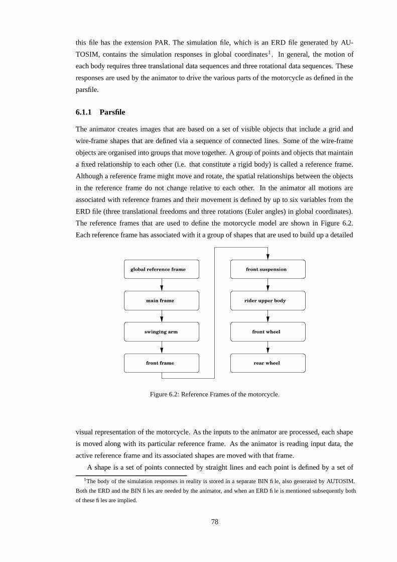
this file has the extension PAR. The simulation file, which is an ERD file generated by AU-
TOSIM, contains the simulation responses in global coordinates1 . In general, the motion of
each body requires three translational data sequences and three rotational data sequences. These
responses are used by the animator to drive the various parts of the motorcycle as defined in the
parsfile.
6.1.1 Parsfile
The animator creates images that are based on a set of visible objects that include a grid and
wire-frame shapes that are defined via a sequence of connected lines. Some of the wire-frame
objects are organised into groups that move together. A group of points and objects that maintain
a fixed relationship to each other (i.e. that constitute a rigid body) is called a reference frame.
Although a reference frame might move and rotate, the spatial relationships between the objects
in the reference frame do not change relative to each other. In the animator all motions are
associated with reference frames and their movement is defined by up to six variables from the
ERD file (three translational freedoms and three rotations (Euler angles) in global coordinates).
The reference frames that are used to define the motorcycle model are shown in Figure 6.2.
Each reference frame has associated with it a group of shapes that are used to build up a detailed
rear wheel
main frame
global reference frame
swinging arm
front frame
front suspension
rider upper body
front wheel
Figure 6.2: Reference Frames of the motorcycle.
visual representation of the motorcycle. As the inputs to the animator are processed, each shape
is moved along with its particular reference frame. As the animator is reading input data, the
active reference frame and its associated shapes are moved with that frame.
A shape is a set of points connected by straight lines and each point is defined by a set of
1The body of the simulation responses in reality is stored in a separate BIN file, also generated by AUTOSIM.
Both the ERD and the BIN files are needed by the animator, and when an ERD file is mentioned subsequently both
of these files are implied.
78
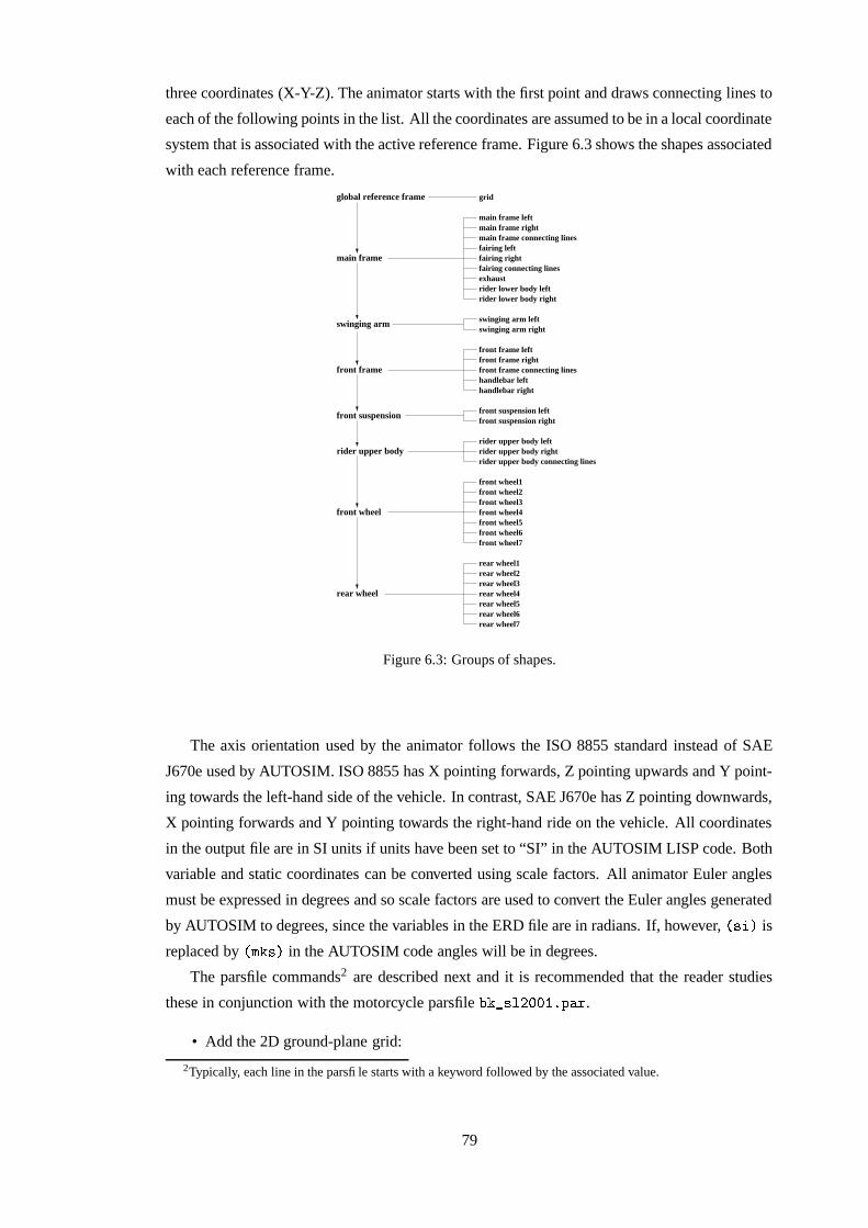
three coordinates (X-Y-Z). The animator starts with the first point and draws connecting lines to
each of the following points in the list. All the coordinates are assumed to be in a local coordinate
system that is associated with the active reference frame. Figure 6.3 shows the shapes associated
with each reference frame.
rear wheel
main frame rightmain frame connecting linesfairing leftfairing rightfairing connecting linesexhaustrider lower body leftrider lower body right
swinging arm leftswinging arm right
front frame leftfront frame rightfront frame connecting lineshandlebar lefthandlebar right
front suspension rightfront suspension left
rider upper body leftrider upper body rightrider upper body connecting lines
front wheel1front wheel2front wheel3front wheel4front wheel5front wheel6front wheel7
rear wheel1rear wheel2rear wheel3rear wheel4rear wheel5rear wheel6rear wheel7
global reference frame grid
main frame
swinging arm
front frame
front suspension
rider upper body
front wheel
main frame left
Figure 6.3: Groups of shapes.
The axis orientation used by the animator follows the ISO 8855 standard instead of SAE
J670e used by AUTOSIM. ISO 8855 has X pointing forwards, Z pointing upwards and Y point-
ing towards the left-hand side of the vehicle. In contrast, SAE J670e has Z pointing downwards,
X pointing forwards and Y pointing towards the right-hand ride on the vehicle. All coordinates
in the output file are in SI units if units have been set to “SI” in the AUTOSIM LISP code. Both
variable and static coordinates can be converted using scale factors. All animator Euler angles
must be expressed in degrees and so scale factors are used to convert the Euler angles generated
by AUTOSIM to degrees, since the variables in the ERD file are in radians. If, however, � � � � is
replaced by � � C � � in the AUTOSIM code angles will be in degrees.
The parsfile commands2 are described next and it is recommended that the reader studies
these in conjunction with the motorcycle parsfile B�C � � � � ���-E � G � .
• Add the 2D ground-plane grid:
2Typically, each line in the parsfile starts with a keyword followed by the associated value.
79
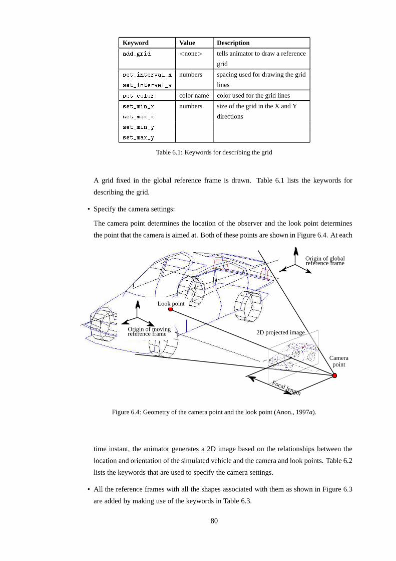
Keyword Value Description������2� ���'�<none> tells animator to draw a reference
grid�����2�������������� �2��numbers spacing used for drawing the grid�����2�������������� �25!
lines�����2�;�+� �+�color name color used for the grid lines�����2�(>����2��numbers size of the grid in the X and Y�����2�(�����2��
directions�����2�(>����25!�����2�(�����25!
Table 6.1: Keywords for describing the grid
A grid fixed in the global reference frame is drawn. Table 6.1 lists the keywords for
describing the grid.
• Specify the camera settings:
The camera point determines the location of the observer and the look point determines
the point that the camera is aimed at. Both of these points are shown in Figure 6.4. At eachChapter 6 The Animator
— 64 —
Origin of global reference frame
Origin of moving reference frame 2D projected image
Camera point
Look point
Focal length
Figure 6.1. Geometry of the camera point and the look point.
The animator allows you, the user, to build and modify descriptions of the system to beanimated. In order to use the program effectively, it is helpful to understand the conceptof a moving reference frame.
Reference FramesThe animator creates images based on a set of visible objects that includes a grid andarbitrary wire-frame shapes defined by a sequence of connected lines. Some of the wire-frame objects are organized into groups that move together. For example, the body of thevehicle is made up of the bumper, rear bumper, left-front door, etc.
A group of points and objects that maintains a fixed relationship (i.e., that constitute arigid body) is called a reference frame. Although the reference frame might move androtate, the spatial relationships between objects in the reference frame do not changerelative to each other. In the animator, all motions are associated with reference frames.Each reference frame has a rectangular coordinate system that is used to describe 3Dlocations of points within that reference frame. For example, Figure 6.1 shows the originsand axes for two reference frames: a global non-moving frame, and a frame that moveswith a vehicle body.
In general, it is not possible to tell how many reference frames exist by looking at a singleimage. However, by observing an animation, it is sometimes possible to see the effects ofall reference frames. For example, the system shown in Figure 6.1 includes six referenceframes:
Figure 6.4: Geometry of the camera point and the look point (Anon., 1997a).
time instant, the animator generates a 2D image based on the relationships between the
location and orientation of the simulated vehicle and the camera and look points. Table 6.2
lists the keywords that are used to specify the camera settings.
• All the reference frames with all the shapes associated with them as shown in Figure 6.3
are added by making use of the keywords in Table 6.3.
80
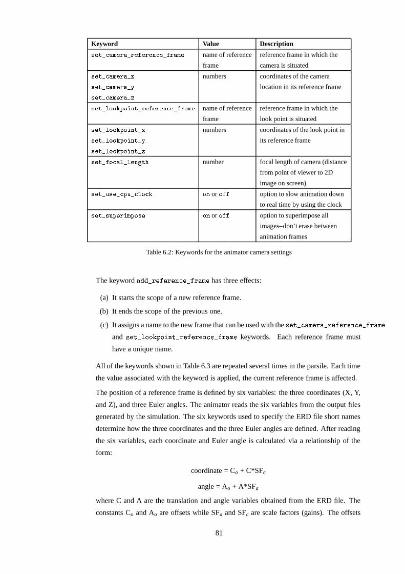
Keyword Value Description�����2�;5�,(�����2����������5��;'��2�����(��name of reference reference frame in which the
frame camera is situated�����2�;5�,(�����2��numbers coordinates of the camera�����2�;5�,(�����2�!
location in its reference frame�����2�;5�,(�����2�������2� +�+1�:�+�������2������������;'��2�����,(��
name of reference reference frame in which the
frame look point is situated�����2� +�+1�:�+�������2��numbers coordinates of the look point in�����2� +�+1�:�+�������2�!
its reference frame�����2� +�+1�:�+�������2�������2��+�;��� �2� ����� ��7
number focal length of camera (distance
from point of viewer to 2D
image on screen)�����25"�����2�;,:�"�2�; �+�;'1 +��or+���
option to slow animation down
to real time by using the clock�����2���"�:���� (�:�+���� +��or+���
option to superimpose all
images–don’t erase between
animation frames
Table 6.2: Keywords for the animator camera settings
The keyword � �� �
� � � � � H � � � � � � has three effects:
(a) It starts the scope of a new reference frame.
(b) It ends the scope of the previous one.
(c) It assigns a name to the new frame that can be used with the � � ��� H �� � � �� � � � � � � H�� � � � �� �and � � � � � F�F�C�GIF � � � � � � � � � � � H � � � � � � keywords. Each reference frame must
have a unique name.
All of the keywords shown in Table 6.3 are repeated several times in the parsile. Each time
the value associated with the keyword is applied, the current reference frame is affected.
The position of a reference frame is defined by six variables: the three coordinates (X, Y,
and Z), and three Euler angles. The animator reads the six variables from the output files
generated by the simulation. The six keywords used to specify the ERD file short names
determine how the three coordinates and the three Euler angles are defined. After reading
the six variables, each coordinate and Euler angle is calculated via a relationship of the
form:
coordinate = Co + C*SFc
angle = Ao + A*SFa
where C and A are the translation and angle variables obtained from the ERD file. The
constants Co and Ao are offsets while SFa and SFc are scale factors (gains). The offsets
81
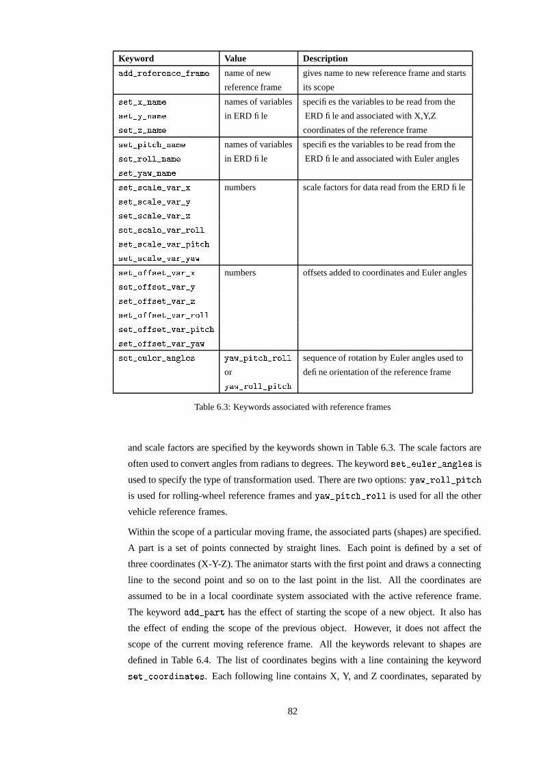
Keyword Value Description������2�������������;���2�����(��name of new gives name to new reference frame and starts
reference frame its scope�����2���25����(��names of variables specifies the variables to be read from the�����2�!�25����(��in ERD file ERD file and associated with X,Y,Z�����2���25����(��
coordinates of the reference frame�����25:I�,��;�7�25���,(��names of variables specifies the variables to be read from the�����2��+� � �25���,(��in ERD file ERD file and associated with Euler angles�����2�!���6�2'���,(��
�����2���;��� ��2�����2��numbers scale factors for data read from the ERD file�����2���;��� ��2�����2�!
�����2���;��� ��2�����2�������2���;��� ��2�����2��+� � �����2���;��� ��2�����25:I����;�7�����2���;��� ��2�����2�!��56�����2�+������5���2������2��
numbers offsets added to coordinates and Euler angles�����2�+������5���2������2�!�����2�+������5���2������2�������2�+������5���2������2��+� � �����2�+������5���2������25:�����;,7�����2�+������5���2������2�!��56�����2���"� ����2����� � ���� !���6�2':I�,��;,7�2��+� �
sequence of rotation by Euler angles used to
or define orientation of the reference frame!���6�25�+� � �2':I�,��;,7
Table 6.3: Keywords associated with reference frames
and scale factors are specified by the keywords shown in Table 6.3. The scale factors are
often used to convert angles from radians to degrees. The keyword � � � � � � ��� ��� � ? ��� � is
used to specify the type of transformation used. There are two options: A � ���F ��� ��G � � H �is used for rolling-wheel reference frames and A � ��G � � H �����F ��� is used for all the other
vehicle reference frames.
Within the scope of a particular moving frame, the associated parts (shapes) are specified.
A part is a set of points connected by straight lines. Each point is defined by a set of
three coordinates (X-Y-Z). The animator starts with the first point and draws a connecting
line to the second point and so on to the last point in the list. All the coordinates are
assumed to be in a local coordinate system associated with the active reference frame.
The keyword ��G � � has the effect of starting the scope of a new object. It also has
the effect of ending the scope of the previous object. However, it does not affect the
scope of the current moving reference frame. All the keywords relevant to shapes are
defined in Table 6.4. The list of coordinates begins with a line containing the keyword
� � ��� H F�F� � � � � � . Each following line contains X, Y, and Z coordinates, separated by
82
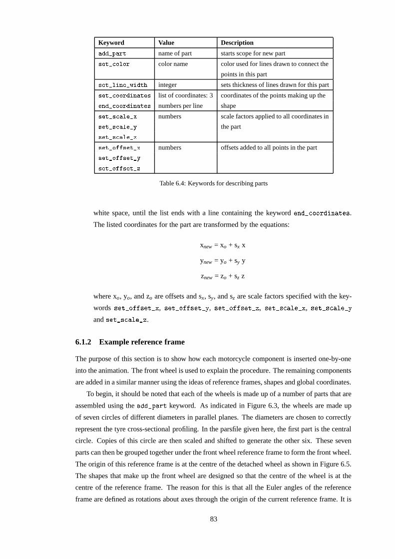
Keyword Value Description������25:����name of part starts scope for new part������2�;�+� +color name color used for lines drawn to connect the
points in this part������2� �������256I�'���7integer sets thickness of lines drawn for this part������2�;�+�+���������������list of coordinates: 3 coordinates of the points making up the������2�;�+�+���������������numbers per line shape������2���;��� ���2��numbers scale factors applied to all coordinates in������2���;��� ���2�!
the part������2���;��� ���2��������2�+����������2��
numbers offsets added to all points in the part������2�+����������2�!������2�+����������2��
Table 6.4: Keywords for describing parts
white space, until the list ends with a line containing the keyword�� � H F�F �� � � � � � .
The listed coordinates for the part are transformed by the equations:
xnew = xo + sx x
ynew = yo + sy y
znew = zo + sz z
where xo, yo, and zo are offsets and sx, sy, and sz are scale factors specified with the key-
words � � � ��F � � � � ��� � , � � ����F � � � � ����A , � � � ��F ��� � � � � � , � � � � � H����� � � , � � � � � H ���� ��Aand � � � � � H����� � � .
6.1.2 Example reference frame
The purpose of this section is to show how each motorcycle component is inserted one-by-one
into the animation. The front wheel is used to explain the procedure. The remaining components
are added in a similar manner using the ideas of reference frames, shapes and global coordinates.
To begin, it should be noted that each of the wheels is made up of a number of parts that are
assembled using the ��G � � keyword. As indicated in Figure 6.3, the wheels are made up
of seven circles of different diameters in parallel planes. The diameters are chosen to correctly
represent the tyre cross-sectional profiling. In the parsfile given here, the first part is the central
circle. Copies of this circle are then scaled and shifted to generate the other six. These seven
parts can then be grouped together under the front wheel reference frame to form the front wheel.
The origin of this reference frame is at the centre of the detached wheel as shown in Figure 6.5.
The shapes that make up the front wheel are designed so that the centre of the wheel is at the
centre of the reference frame. The reason for this is that all the Euler angles of the reference
frame are defined as rotations about axes through the origin of the current reference frame. It is
83
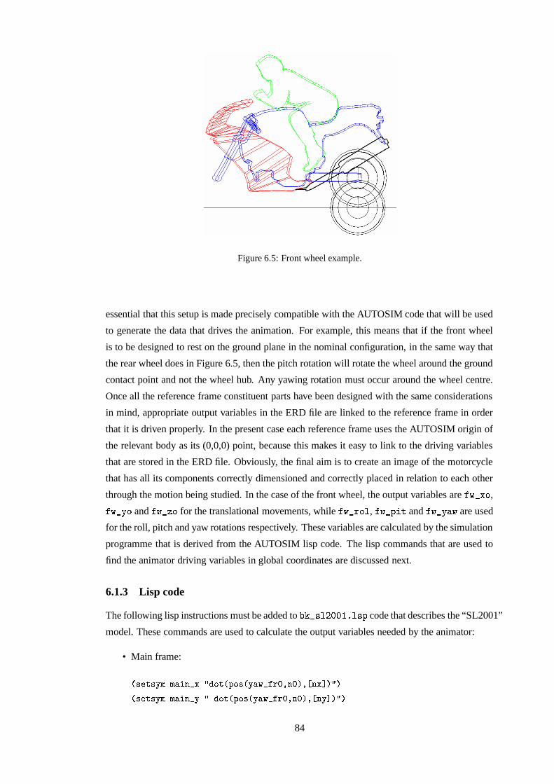
Figure 6.5: Front wheel example.
essential that this setup is made precisely compatible with the AUTOSIM code that will be used
to generate the data that drives the animation. For example, this means that if the front wheel
is to be designed to rest on the ground plane in the nominal configuration, in the same way that
the rear wheel does in Figure 6.5, then the pitch rotation will rotate the wheel around the ground
contact point and not the wheel hub. Any yawing rotation must occur around the wheel centre.
Once all the reference frame constituent parts have been designed with the same considerations
in mind, appropriate output variables in the ERD file are linked to the reference frame in order
that it is driven properly. In the present case each reference frame uses the AUTOSIM origin of
the relevant body as its (0,0,0) point, because this makes it easy to link to the driving variables
that are stored in the ERD file. Obviously, the final aim is to create an image of the motorcycle
that has all its components correctly dimensioned and correctly placed in relation to each other
through the motion being studied. In the case of the front wheel, the output variables are�� � � F ,
�� ��AIF and
�� � ��F for the translational movements, while
�� ��IF � ,
�� ��G � � and
�� ��A � are used
for the roll, pitch and yaw rotations respectively. These variables are calculated by the simulation
programme that is derived from the AUTOSIM lisp code. The lisp commands that are used to
find the animator driving variables in global coordinates are discussed next.
6.1.3 Lisp code
The following lisp instructions must be added to B�C�� � � � ���-E � � ��G code that describes the “SL2001”
model. These commands are used to calculate the output variables needed by the animator:
• Main frame:
��������,!5($(�������2��%/���+� �#:�+��-�#!���6�2�(� � �(��� � � �(������/����������,!5($(�������2�!%/�'��+�� �#:�+��9��!���6�2�� � � � ��� � � ��! ����/��
84
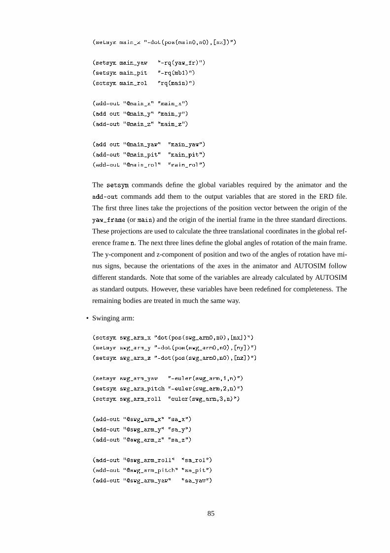
��������,!5($(�������2��8/�'��+�� �#:�+��9� (������ � � � ��� � � �(� ����/�
��������,!5($(�������2�!���6 /�, � ��!���6�2�����/����������,!5($(�������25:I�,� /�, � � (�*-4���/���������,!5($(�������2��+� /.�� � (���������/�
���������'+�"��8/ ��(�������2��9/ /�(�������2��9/�����������'+�"��8/ ��(�������25!9/ /�(�������2�!9/�����������'+�"��8/ ��(�������2��I/ /�(�������2��I/��
���������'+�"��8/ ��(�������25!���6-/ /�(����.��2�!���69/����������'+�"��8/ ��(�������2':I�,�9/ /�(����.��25:I�,�I/����������'+�"��8/ ��(�������25�+� �/ /�(����.��2��+� �/�
The � � � ��A � commands define the global variables required by the animator and the >=�F � � commands add them to the output variables that are stored in the ERD file.
The first three lines take the projections of the position vector between the origin of the
A � � � � �� � (or� �
� ) and the origin of the inertial frame in the three standard directions.
These projections are used to calculate the three translational coordinates in the global ref-
erence frame � . The next three lines define the global angles of rotation of the main frame.
The y-component and z-component of position and two of the angles of rotation have mi-
nus signs, because the orientations of the axes in the animator and AUTOSIM follow
different standards. Note that some of the variables are already calculated by AUTOSIM
as standard outputs. However, these variables have been redefined for completeness. The
remaining bodies are treated in much the same way.
• Swinging arm:
��������,!5()�,6� �2�5(I2�� /���+� � :�+��-����6� �2��,( � � � ��� ��� �+� ����/���������,!5()�,6� �2�5(I2�! /�'��+� �#:�+��-�&�,6� �2��55( � � � ��� ��� ��! ����/5���������,!5()�,6� �2�5(I2���/�'��+� �#:�+��-�&�,6� �2��55( � � � ��� ��� �(� ����/5�
��������,!5()�,6� �2�5(I2�!���6 /�5��"� �� ����6� �2��'( ��4 � �I��/����������,!5()�,6� �2�5(I25:��,��;,7�/�5��"� �� ����6� �2��'( � � � �I��/����������,!5()�,6� �2�5(I2��+� � /,��"� � ���,6� �2��5( � � � ����/��
���������'+�"��8/ ���,6� �2���5(I2��9/ /�����2��9/����������'+�"��8/ ���,6� �2���5(I2�!9/ /�����25!9/����������'+�"��8/ ���,6� �2���5(I2��I/ /�����2��I/�
���������'+�"��8/ ���,6� �2���5(I2��+� � �/ /�����2��+� �/�����������'+�"��8/ ���,6� �2���5(I25:I����;,7-/ /�����25:I�,�9/�����������'+�"��8/ ���,6� �2���5(I2�!��56-/ /�����2�!���6-/��
85
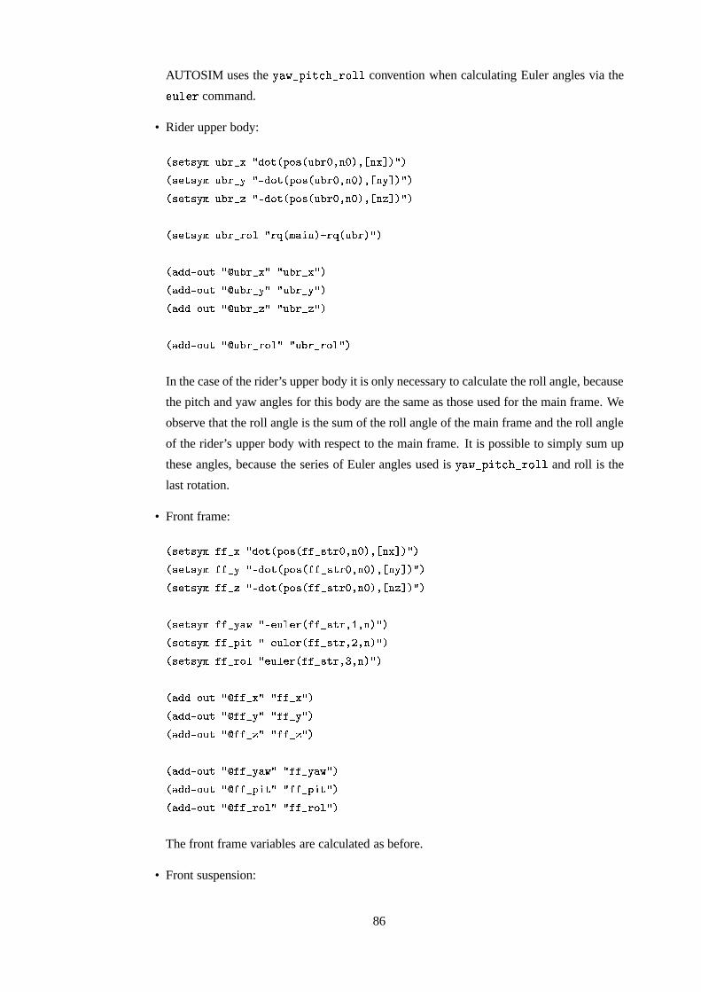
AUTOSIM uses the A � ��G � � H � � ��F ��� convention when calculating Euler angles via the����� � command.
• Rider upper body:
��������,!5( "�*��2��%/���+� � :�+��-�#"�*� � � � ��� ��� �(� ����/���������,!5( "�*��25!%/�'��+� �#:�+��-� "�*� � � � ��� ��� ��! ����/���������,!5( "�*��2��8/�'��+� �#:�+��-� "�*� � � � ��� ��� �(� ����/�
��������,!5( "�*��25�+� /. � � (����.�I� ��� �#"�*����/�
���������'+�"��8/ �5"�*��2��I/$/�"�*��2��9/����������'+�"��8/ �5"�*��2�!I/$/�"�*��25!9/����������'+�"��8/ �5"�*��2���/$/�"�*��2��I/�
���������'+�"��8/ �5"�*��2��+� �/ /�"�*��2��+� �/�
In the case of the rider’s upper body it is only necessary to calculate the roll angle, because
the pitch and yaw angles for this body are the same as those used for the main frame. We
observe that the roll angle is the sum of the roll angle of the main frame and the roll angle
of the rider’s upper body with respect to the main frame. It is possible to simply sum up
these angles, because the series of Euler angles used is A � ��G � � H � ��IF ��� and roll is the
last rotation.
• Front frame:
��������,!5(�����2��)/���+� �#:�+��-������2��'��(� � � ��� ��� �+� ����/5���������,!5(�����2�!)/�,��+� �#:�+��-������2��'��(� � � ��� � � ��!�����/���������,!5(�����2��%/�,��+� �#:�+��-������2��'��(� � � ��� � � �(� ����/�
��������,!5(�����2�!���6)/�5��"� �� ������2��'�� �.4 � ����/����������,!5(�����25:��,�%/�5��"� �� ������2��'�� � � � ����/����������,!5(�����2��+� �/,��"� � ������2��'��"� � � �I��/�
���������'+�"��8/ �����2��9/$/.����2��9/�����������'+�"��8/ �����2�!9/$/.����2�!9/�����������'+�"��8/ �����2��I/$/.����2��I/��
���������'+�"��8/ �����2�!��56-/ /�����2�!���6-/�����������'+�"��8/ �����25:I���9/ /�����25:I�,�9/�����������'+�"��8/ �����2��+� �/ /�����2��+� �/��
The front frame variables are calculated as before.
• Front suspension:
86
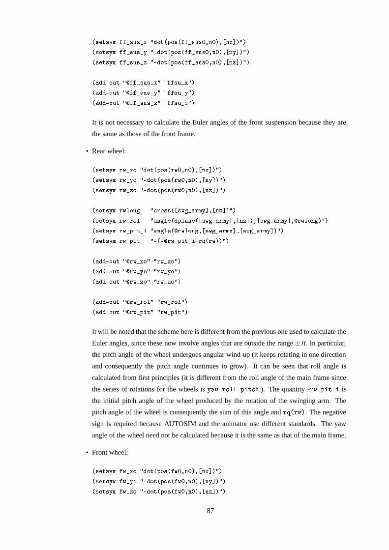
��������,!5(�����2���"��2��8/.��+� �#:�+��-������2��,"���� � � ��� ��� � ������/����������,!5(�����2���"��2�!8/��'��+� � :�+��-������2��,"�� � � � ��� ��� ��! ����/���������,!5(�����2���"��2�� /��'��+� � :�+��-������2��,"�� � � � ��� ��� � � ����/�
���������'+�"��8/ �����2��,"��2��9/ /������,"�2��9/����������'+�"��8/ �����2��,"��2�!9/ /������,"�2�!9/����������'+�"��8/ �����2��,"��2��I/ /������,"�2��I/�
It is not necessary to calculate the Euler angles of the front suspension because they are
the same as those of the front frame.
• Rear wheel:
��������,!5( �6�2���+ /���+� � :�+��-��6 � � � ��� ��� � ������/����������,!5( �6�2�!�+ /�'��+� �#:�+��-�#�6 � � � ��� ��� ��! ����/���������,!5( �6�2���+ /�'��+� �#:�+��-�#�6 � � � ��� ��� � � ����/�
��������,!5( �6� �+5�� /5;'�+����9� ���,6� �2��5(�! � � � �(� ����/���������,!5( �6�2��+� /����� � �� ���:� ��5��� � ���.6� �2��5(�! � � � �(� ��� ������6� �2��55(�! � � ��6� +5�� ���/5���������,!5( �6�25:��,��2�� /����� � �� � ��6� +��� "���#�,6� �2�5( ��� � ���,6� �2���'(�! ����/���������,!5( �6�25:��,� /��9�.� �6�25:I�,��2�� ��� ��6�����/�
���������'+�"��8/ ���6�2���+�/$/.�6�2���+�/����������'+�"��8/ ���6�2�!�+�/$/.�6�2�!�+�/����������'+�"��8/ ���6�2���+�/$/.�6�2���+�/�
���������'+�"��8/ ���6�2��+� �/ /.�6�2��+� �/�����������'+�"��8/ ���6�25:I���9/ /.�6�25:I�,�9/��
It will be noted that the scheme here is different from the previous one used to calculate the
Euler angles, since these now involve angles that are outside the range ±π . In particular,
the pitch angle of the wheel undergoes angular wind-up (it keeps rotating in one direction
and consequently the pitch angle continues to grow). It can be seen that roll angle is
calculated from first principles (it is different from the roll angle of the main frame since
the series of rotations for the wheels is A � � ��F ��� ��G � � H � .). The quantity - � � ��G � � � � is
the initial pitch angle of the wheel produced by the rotation of the swinging arm. The
pitch angle of the wheel is consequently the sum of this angle and ��� � � � � . The negative
sign is required because AUTOSIM and the animator use different standards. The yaw
angle of the wheel need not be calculated because it is the same as that of the main frame.
• Front wheel:
��������,!5(��6�2���+ /���+� � :�+��-����6 � � � ��� ��� � ������/����������,!5(��6�2�!�+ /�'��+� �#:�+��-���6 � � � ��� ��� ��! ����/���������,!5(��6�2���+ /�'��+� �#:�+��-���6 � � � ��� ��� � � ����/�
87
��������,!5(��6� �+5�� /5;'�+����9� � ����2��,"��'!�� ��� �(� ����/5���������,!5(��6�2��+� /����� � �� ���:� ��5��� � � ���2���"��'!�� ��� �(� ��� ��� ����2���"���!�� � ����6� �+��� ���/����������,!5(��6�25:��,��2�� /����� � �� � ���6� +��� "��� ����2���"�� � � � � ����2��."��,! ����/���������,!5(��6�25:��,� /��9�.� ����6�25:I�,��2�� ��� ����6�����/�
���������'+�"��8/ ��6�2���+�/$/��6�2���+�/����������'+�"��8/ ��6�2�!�+�/$/��6�2�!�+�/����������'+�"��8/ ��6�2���+�/$/��6�2���+�/�
���������'+�"��8/ ��6�2��+� �/ /��6�2��+� �/�����������'+�"��8/ ��6�25:I���9/ /��6�25:I�,�9/��
6.1.4 Running the animator
To run the animator the following items are needed:
• The animator executable file�� � �IF� � ���� (this can be downloaded from the author’s
website http://www.ee.ic.ac.uk/control/motorcycles).
• The parsile B�C�� � � � ���-E � G � (this can be downloaded from the same website).
• The simulation files����� G ��� � � � and
��� � G ��� �#B � � . These files can be downloaded
from the above website, or they can be generated by patching the Lisp code B�C�� � � � ���-E � � ��G .
The instructions that generate the required data in global coordinates should be placed just
before the � � � � � ��� � command. A new data file must be generated by loading the modi-
fied AUTOSIM code and running the associated simulation file.
The animation can be run as follows:
• Start the animator by running the executable file�� � ��F � � ��� � .
• Go to the file roll-down menu in the animator window, click on Open Parsfile and select
the parsfile B�C � � � � ���-E � G � .
• Find and select the ERD file (����� G ��� � � �� ) in the same window.
• After all the files are loaded the animation can be started by going to the Animation roll-
down menu and clicking on Start From Beginning.
88

Part III
Results
89
The theoretical techniques that have been presented will now be employed for the inves-
tigation of the stability of motorcycles under acceleration and deceleration, and the effects on
motorcycle stability from road forcing. These issues are treated in Chapters 7 and 8 respectively.
The work presented was also covered in (Limebeer et al., 2001) and (Limebeer et al., 2002).
90
Chapter 7
The stability of motorcycles under
acceleration and braking
The dynamic properties of single-track vehicles under acceleration and deceleration have not
received much attention in the literature, and as far the present author is aware, the only work
in this area is that given in (Sharp, 1976b). The analysis techniques employed in that study
were introduced earlier in the context of the jack-knifing of articulated vehicles (Hales, 1965),
but by contemporary standards these are simplistic because they only consider the ‘inertial ef-
fects’ of acceleration. Also, the vehicle model used was simple and the absence of a suspension
system meant that the effects of acceleration on the tyre loads were not treated accurately. A
further weakness was that the influence of load on the tyre shear forces was not known with any
precision.
In the present chapter an attempt is made to evaluate the dynamic behaviour of motorcycles
under acceleration and deceleration using modern theoretical techniques. The main focus is on
the behaviour of the wobble and weave modes and the motorcycle model employed is the one
described in Chapter 5.
7.1 Stability/instability of time varying systems
Mathematical models of motorcycles under acceleration and deceleration are time varying sys-
tems and special methods are required to examine their dynamic stability properties. The pur-
pose of this short section is to review briefly some of the stability/instability properties of time-
varying systems.
It is well known that the nth-order order differential equation:
xxx(t) = AAAxxx(t) xxx(0) = xxxo,
has solution:
xxx(t) =n
∑i=1
wieλitv∗i xxxo
91
in which the λi’s are the eigenvalues of the constant matrix AAA (AAA is assumed to be diagonalisable)
(Strang, 1988), and the wi’s and vi’s are the corresponding eigenvectors and dual eigenvectors
respectively. These solutions will vanish asymptotically if Re(λi) < 0. In other words, for an
arbitrary xxxooo the solutions of this equation converge to zero if (and only if) all the eigenvalues
of AAA have negative real parts. In general, the stability properties of linear time varying systems
cannot be tested using the eigenvalues in this way. For example, the matrix
AAA(t) =
[
−1 e2t
0 −1
]
has both its eigenvalues at −1 for all t, but the corresponding system xxx(t) = AAA(t)xxx(t) is unstable
in the sense that for some initial conditions limt→∞ xxx(t) is unbounded (Kailath, 1980). There-
fore, in general, there is no significance to the concept of a ‘mode’, or a ‘time varying natural
frequency’ in the case of time-variant linear systems. Consider:
xxx(t) = AAA(t)xxx(t), xxxo = xxx(0).
Provided AAA(t) is small enough for all t ≥ 0, it would be expected intuitively that the time-
varying system will be stable provided that for each frozen time t, the (frozen-time) system AAA(t)
is stable. It is known (Desoer, 1969) that if the eigenvalues of AAA(t) have real parts that are
sufficiently negative for all t ≥ 0, and supt≥0 ‖AAA(t)‖ is sufficiently small, then the solutions of
xxx(t) = AAA(t)xxx(t) go to zero as t → ∞.
There might also be trouble when predicting instability using the frozen-time eigenvalues
of AAA(t). If AAA(t) has at least one frozen-time eigenvalue with positive real part, the solutions
of xxx(t) = AAA(t)xxx(t) may be stable. One would expect that if AAA(t) has eigenvalues in the right
half plane, then the system xxx(t) = AAA(t)xxx(t) will have unbounded solutions if supt≥0 ‖AAA(t)‖ is
sufficiently small. This is indeed the case provided no eigenvalue crosses the imaginary axis
(Skoog and Lau, 1972) as time changes. If eigenvalues are allowed to cross the imaginary
axis, then even though there is always an eigenvalue with positive real part, the system can be
asymptotically stable for arbitrarily small supt≥0 ‖AAA(t)‖. Consider the matrix (Skoog and Lau,
1972)
AAA(t) =
[
−1+α cos ωt sinωt α cos2 ωt +ω−α sin2 ωt −ω −1−α cosωt sinωt
]
.
The corresponding transition matrix φ(t, t0) is given by
Φ(t, to) = e−(t−t0)
[
cosωt sin ωt
−sinωt cosωt
][
1 α(t − t0)
0 1
][
cosωt0 −sinωt0
sin ωt0 cos ωt0
]
and so with this AAA(t) all the corresponding equation solutions are exponentially bounded. It is
easy to check that the eigenvalues of AAA(t) are time independent and given by
λ = −1±√
−αω −ω2.
92
Setting ω = 1 and α =−5 the eigenvalues of AAA(t) are at +1 and −3 for all time. Note, however,
that for any α < −2, if
0 < ω < −α2− 1
2
√
α2 −4
or
ω > −α2
+12
√
α2 −4,
then the eigenvalues of AAA(t) have negative real parts. Thus when AAA(t) is varying either slowly or
rapidly, the eigenvalues of AAA(t) correctly predict the stability properties of the system. When ωlies between the aforementioned limits,
−α2− 1
2
√
α2 −4 < ω < −α2
+12
√
α2 −4
they do not.
The idea of a ‘mode’ will be used for the linear time varying systems and the eigenvalues of
frozen-time linearised models will be used to infer stability properties, but it is recognised that
this must be done with due caution.
7.2 Results
Root-loci and nonlinear simulation results are presented that show the effects of acceleration
and deceleration on motorcycle stability. The main emphasis will be on the weave and wobble
modes, as these are the dominant ones under the acceleration/deceleration conditions of interest
here. The nonlinear simulation results come directly from the FORTRAN simulation codes
generated by AUTOSIM. The root-locus plots are generated via the eigenvalues of frozen-time
symbolic linearised state-space models (also generated by AUTOSIM). The evaluation of the
linearised state-space model matrices requires information about the frozen-time values of the
various model states—this information is provided by the nonlinear simulation codes. In order
to generate a root-locus plot, the nonlinear simulation model is accelerated/decelerated over the
speed range of interest. These data had to be checked to ensure: (a) that the rear wheel did not
leave the ground (thereby indicating a stoppie), (b) that the front wheel did not leave the ground
(thereby indicating a wheelie), (c) that the tyres did not undergo longitudinal saturation; and
(d) that the engine power did not exceed 65 kW. The saturation condition was checked via the
negativity, or otherwise, of the test force:
Fcheck = 0.8Fload + |Flong| (7.1)
in which Fload is the tyre normal load and is always negative, while Flong is the tyre longitudinal
force and can be positive or negative. If Fcheck ≥ 0, the tyre was deemed to have saturated and the
associated simulation data was disregarded. The root-locus plots that correspond to the constant-
speed cases were generated by accelerating the machine very gradually over the speed range of
interest.
93
7.2.1 Straight running on an incline
The results in this chapter begin by building on the intuitive ideas in (Hales, 1965) and (Sharp,
1976b). To do this, the stability properties of the machine on inclined surfaces are studied
at constant speed. The idea is that ascending/descending inclined running surfaces generates
gravitational forces that mimic the inertial forces associated with acceleration/deceleration con-
ditions, respectively. It should also be noted that the constant-speed condition means that there
is no temporal variation in the aerodynamic loading as the speed changes and that the associated
linearised models are time-invariant. There is therefore no need to consider the complications
associated with the stability testing, via the eigenvalues of frozen-time linearised models, of
time-varying systems. Figure 7.1 shows root-locus plots for the cases of straight running, at
constant speed, on both level and inclined smooth surfaces. The speed ranges associated with
the various cases are dictated by the limiting conditions referred to above. The first thing to
note is that the wobble mode is destabilised significantly on downhill (as opposed to uphill)
inclinations. It can also be seen that the wobble mode is marginally more stable under rear-
wheel-dominated braking. It is common experience that one should use rear-wheel-dominated
braking on down-hill slopes at very low speeds, especially in slippery road conditions. Fig-
ure 7.1 also shows that inclined road surfaces have very little influence on the weave mode. At
very low speeds, the weave mode forms at higher than usual speed under front-wheel dominated
braking. Intuitively, this makes the machine harder to control under these conditions, because it
tends to just ‘fall over’, rather than undergo an unstable low frequency oscillation. This could be
the reason for the rider training advice that at very low speed the machine should be controlled
by alternating the throttle and rear brake.
7.2.2 Acceleration studies
Figures 7.2, 7.3 and 7.4 consider the effects of acceleration on motorcycle stability. As ex-
pected, the general trends follow those associated with the results obtained for constant speeds
on ascending slopes. The reason for this is that the inertial forces act in the same direction in
the acceleration case as the gravity forces do in the uphill case. Figure 7.2 shows that the weave
mode is hardly affected by the acceleration, while the wobble mode is substantially more heavily
damped. These effects probably account for the good ‘feel’ associated with powerful machines
under firm acceleration.
Figure 7.3 shows the effect of speed on the aerodynamic drag, the tyre loads, the drive torque
and the rear tyre saturation. The aerodynamic drag increases quadratically with speed as does
the required drive moment. The aerodynamic drag also tends to load the rear wheel, while
correspondingly lightening the normal load on the front tyre. Also, as expected, the increased
drive torque and longitudinal tyre force bring the rear tyre closer to saturation.
In Section 7.1 the reader was reminded that the stability of linear time-varying systems
cannot be tested using the frozen-time eigenvalues of AAA(t) alone. With that warning in mind,
the transient behaviour of the machine was examined with the nonlinear simulation model and
94
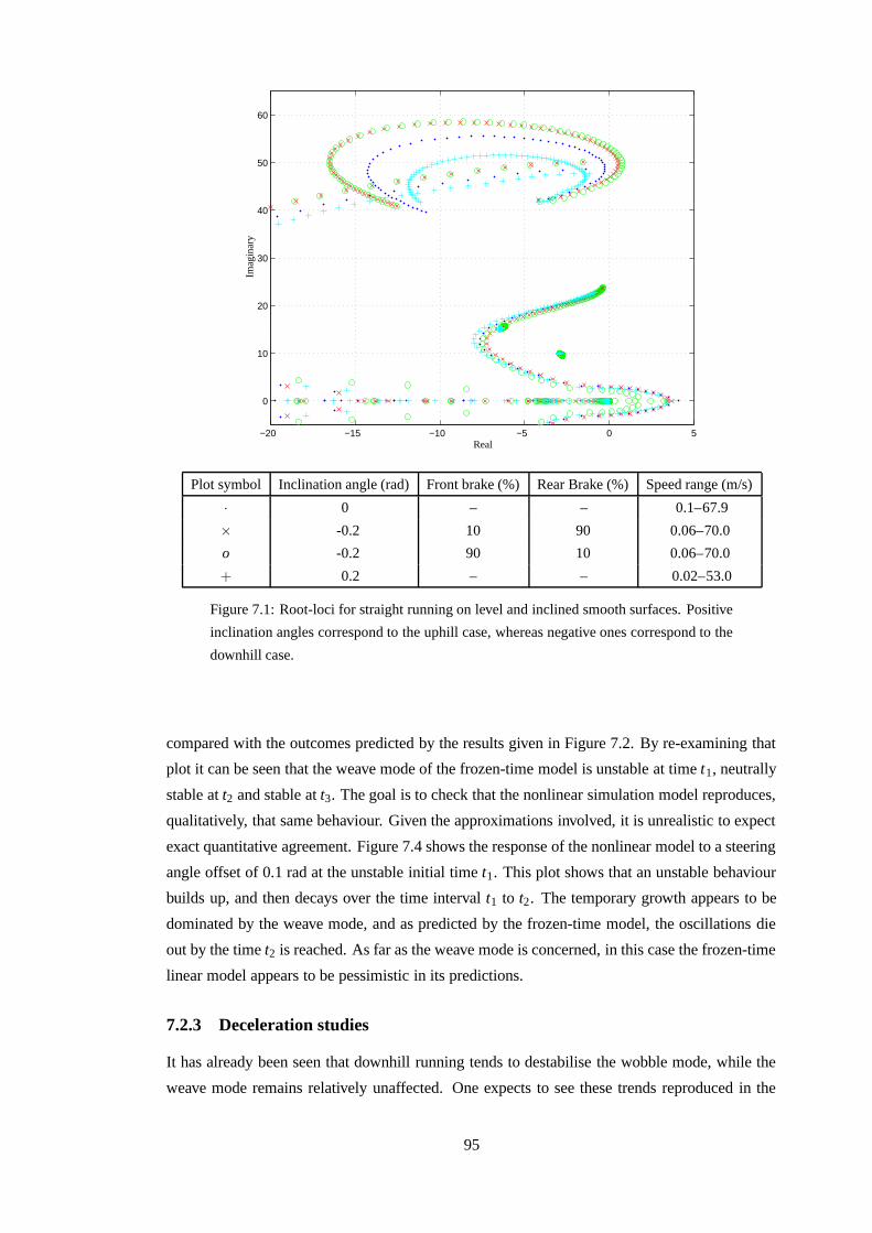
−20 −15 −10 −5 0 5
0
10
20
30
40
50
60
PSfrag replacements
Real
Imag
inar
y
Plot symbol Inclination angle (rad) Front brake (%) Rear Brake (%) Speed range (m/s)
· 0 – – 0.1–67.9
× -0.2 10 90 0.06–70.0
o -0.2 90 10 0.06–70.0
+ 0.2 – – 0.02–53.0
Figure 7.1: Root-loci for straight running on level and inclined smooth surfaces. Positive
inclination angles correspond to the uphill case, whereas negative ones correspond to the
downhill case.
compared with the outcomes predicted by the results given in Figure 7.2. By re-examining that
plot it can be seen that the weave mode of the frozen-time model is unstable at time t1, neutrally
stable at t2 and stable at t3. The goal is to check that the nonlinear simulation model reproduces,
qualitatively, that same behaviour. Given the approximations involved, it is unrealistic to expect
exact quantitative agreement. Figure 7.4 shows the response of the nonlinear model to a steering
angle offset of 0.1 rad at the unstable initial time t1. This plot shows that an unstable behaviour
builds up, and then decays over the time interval t1 to t2. The temporary growth appears to be
dominated by the weave mode, and as predicted by the frozen-time model, the oscillations die
out by the time t2 is reached. As far as the weave mode is concerned, in this case the frozen-time
linear model appears to be pessimistic in its predictions.
7.2.3 Deceleration studies
It has already been seen that downhill running tends to destabilise the wobble mode, while the
weave mode remains relatively unaffected. One expects to see these trends reproduced in the
95
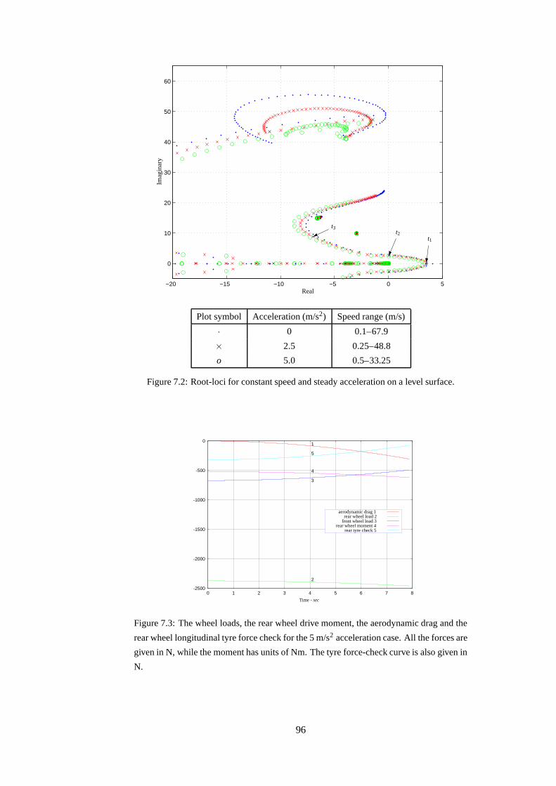
−20 −15 −10 −5 0 5
0
10
20
30
40
50
60
PSfrag replacements
Real
Imag
inar
y
t1t2
t3
Plot symbol Acceleration (m/s2) Speed range (m/s)
· 0 0.1–67.9
× 2.5 0.25–48.8
o 5.0 0.5–33.25
Figure 7.2: Root-loci for constant speed and steady acceleration on a level surface.
-2500
-2000
-1500
-1000
-500
0
0 1 2 3 4 5 6 7 8
1
5
4
3
2
PSfrag replacements
Time - sec
aerodynamic drag 1rear wheel load 2
front wheel load 3rear wheel moment 4
rear tyre check 5
Figure 7.3: The wheel loads, the rear wheel drive moment, the aerodynamic drag and the
rear wheel longitudinal tyre force check for the 5 m/s2 acceleration case. All the forces are
given in N, while the moment has units of Nm. The tyre force-check curve is also given in
N.
96

-0.15
-0.1
-0.05
0
0.05
0.1
0.15
1 2 3 4 5 6
PSfrag replacements
Time - sec
yaw angleroll angle
steer angle
t1 = 0 t2 = 3.04 t3 = 7
Figure 7.4: Transient response of the weave mode for the 2.5 m/s2 acceleration case. The
initial speed is 0.25 m/s and the initial steer angle offset is 0.1 rad; the speed at t2 is 7.85
m/s, while that at t3 is 17.75 m/s. The time origin corresponds to the point t1 in Figure 7.2,
and the other two time-marker points are labelled as t2 and t3.
deceleration studies, because the inertial forces in deceleration are equivalent to the gravitational
forces in the downhill case. Figure 7.5 shows that these expectations are substantially true. It can
be seen from this figure that the wobble mode becomes significantly less stable under braking
and the effects become exaggerated as the deceleration rate increases. This figure also shows that
the weave mode remains relatively unaffected by braking—as with the downhill case, the weave
mode is affected most at very low speed. Figure 7.6 shows the anticipated changes in the wheel
loads and wheel drive moments under braking. As expected, the bulk of the motorcycle’s weight
is carried by the front wheel, as is the bulk of the braking torque (under front-wheel-dominated
braking). Note how the braking moment increases as the speed drops. This is explained by the
fact that the aerodynamic drag does most of the high-speed braking, but this task is then taken
over by the brakes as the aerodynamic drag reduces. Figure 7.7 is used to check the stability
interpretations being given to the root-loci in Figure 7.5. As the speed decreases, the 2.5 m/s2
wobble mode moves through the time markers t1, t2, t3 and t4 in that order. On the basis of the
frozen-time root-locus analysis, the wobble mode is deemed unstable at t1, neutrally stable at t2
and stable at times t3 and t4. Figure 7.7 shows the response of the nonlinear model to a steer
angle offset of 0.0001 rad applied at time t1. As expected, the oscillations grow until t3 and decay
thereafter. This figure is therefore in qualitative agreement with Figure 7.51. Figure 7.8 shows
the response of the nonlinear simulation model to a small roll angle offset of 0.0005 rad that
is applied at t1 in Figure 7.5. The yaw angle, roll angle and steering head twist angle all show
1The author’s supervisor has repeatedly noted a marked steering shimmy at about 60 mile/h under firm braking—
this was not caused by disk run out! At the time he was riding a Kawasaki ZX-9R on Snetterton race track in Norfolk
and was braking down from about 140 mile/h. This anecdotal evidence is in broad agreement with the theoretical
results presented here.
97
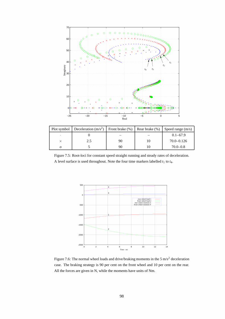
−25 −20 −15 −10 −5 0 5
0
10
20
30
40
50
60
70
PSfrag replacements
Real
Imag
inar
yt1
t2t3t4
Plot symbol Deceleration (m/s2) Front brake (%) Rear brake (%) Speed range (m/s)
· 0 – – 0.1–67.9
× 2.5 90 10 70.0–0.126
o 5 90 10 70.0–0.8
Figure 7.5: Root-loci for constant speed straight running and steady rates of deceleration.
A level surface is used throughout. Note the four time markers labelled t1 to t4.
-2500
-2000
-1500
-1000
-500
0
500
0 2 4 6 8 10 12 14
4
3
1
2
PSfrag replacements
Time - sec
rear wheel load 1front wheel load 2
rear wheel moment 3front wheel moment 4
Figure 7.6: The normal wheel loads and drive/braking moments in the 5 m/s2 deceleration
case. The braking strategy is 90 per cent on the front wheel and 10 per cent on the rear.
All the forces are given in N, while the moments have units of Nm.
98
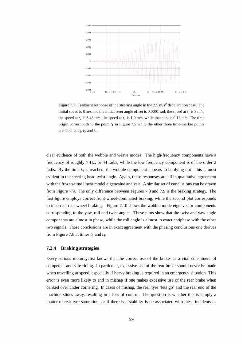
-0.004
-0.003
-0.002
-0.001
0
0.001
0.002
0.003
0.004
0.005
0.5 1 1.5 2 2.5 3
PSfrag replacements
Time - sec
t1 = 0 t2 = 0.61 t3 = 2.44 t4 = 3.15
Figure 7.7: Transient response of the steering angle in the 2.5 m/s2 deceleration case. The
initial speed is 8 m/s and the initial steer angle offset is 0.0001 rad; the speed at t1 is 8 m/s;
the speed at t2 is 6.48 m/s; the speed at t3 is 1.9 m/s, while that at t4 is 0.13 m/s. The time
origin corresponds to the point t1 in Figure 7.5 while the other three time-marker points
are labelled t2, t3 and t4.
clear evidence of both the wobble and weave modes. The high-frequency components have a
frequency of roughly 7 Hz, or 44 rad/s, while the low frequency component is of the order 2
rad/s. By the time t4 is reached, the wobble component appears to be dying out—this is most
evident in the steering head twist angle. Again, these responses are all in qualitative agreement
with the frozen-time linear model eigenvalue analysis. A similar set of conclusions can be drawn
from Figure 7.9. The only difference between Figures 7.8 and 7.9 is the braking strategy. The
first figure employs correct front-wheel-dominated braking, while the second plot corresponds
to incorrect rear wheel braking. Figure 7.10 shows the wobble mode eigenvector components
corresponding to the yaw, roll and twist angles. These plots show that the twist and yaw angle
components are almost in phase, while the roll angle is almost in exact antiphase with the other
two signals. These conclusions are in exact agreement with the phasing conclusions one derives
from Figure 7.8 at times t3 and t4.
7.2.4 Braking strategies
Every serious motorcyclist knows that the correct use of the brakes is a vital constituent of
competent and safe riding. In particular, excessive use of the rear brake should never be made
when travelling at speed, especially if heavy braking is required in an emergency situation. This
error is even more likely to end in mishap if one makes excessive use of the rear brake when
banked over under cornering. In cases of mishap, the rear tyre ‘lets go’ and the rear end of the
machine slides away, resulting in a loss of control. The question is whether this is simply a
matter of rear tyre saturation, or if there is a stability issue associated with these incidents as
99
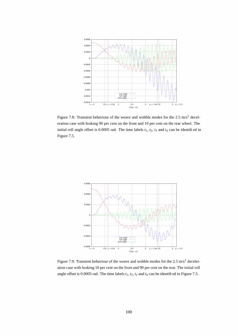
-0.0014
-0.0012
-0.001
-0.0008
-0.0006
-0.0004
-0.0002
0
0.0002
0.0004
0.0006
0.5 1 1.5 2 2.5 3
PSfrag replacements
Time - sec
t1 = 0 t2 = 0.61 t3 = 2.44 t4 = 3.15
yaw angleroll angle
twist angle
Figure 7.8: Transient behaviour of the weave and wobble modes for the 2.5 m/s2 decel-
eration case with braking 90 per cent on the front and 10 per cent on the rear wheel. The
initial roll angle offset is 0.0005 rad. The time labels t1, t2, t3 and t4 can be identified in
Figure 7.5.
-0.0006
-0.0004
-0.0002
0
0.0002
0.0004
0.0006
0.5 1 1.5 2 2.5 3
PSfrag replacements
Time - sec
t1 = 0 t2 = 0.61 t3 = 2.44 t4 = 3.15
yaw angleroll angle
twist angle
Figure 7.9: Transient behaviour of the weave and wobble modes for the 2.5 m/s2 deceler-
ation case with braking 10 per cent on the front and 90 per cent on the rear. The initial roll
angle offset is 0.0005 rad. The time labels t1, t2, t3 and t4 can be identified in Figure 7.5.
100
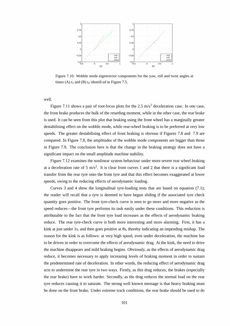
−0.5 0 0.5 1−0.5
−0.25
0
0.25
0.5
0.75
1
(A)−0.5 0 0.5 1
−0.5
−0.25
0
0.25
0.5
0.75
1
(B)
PSfrag replacements yawyawrollrolltwisttwist
Figure 7.10: Wobble mode eigenvector components for the yaw, roll and twist angles at
times (A) t3 and (B) t4 identified in Figure 7.5.
well.
Figure 7.11 shows a pair of root-locus plots for the 2.5 m/s2 deceleration case. In one case,
the front brake produces the bulk of the retarding moment, while in the other case, the rear brake
is used. It can be seen from this plot that braking using the front wheel has a marginally greater
destabilising effect on the wobble mode, while rear-wheel braking is to be preferred at very low
speeds. The greater destabilising effect of front braking is obvious if Figures 7.8 and 7.9 are
compared. In Figure 7.8, the amplitudes of the wobble mode components are bigger than those
in Figure 7.9. The conclusion here is that the change in the braking strategy does not have a
significant impact on the small amplitude machine stability.
Figure 7.12 examines the nonlinear system behaviour under more severe rear wheel braking
at a deceleration rate of 5 m/s2. It is clear from curves 1 and 2 that there is a significant load
transfer from the rear tyre onto the front tyre and that this effect becomes exaggerated at lower
speeds, owing to the reducing effects of aerodynamic loading.
Curves 3 and 4 show the longitudinal tyre-loading tests that are based on equation (7.1);
the reader will recall that a tyre is deemed to have begun sliding if the associated tyre check
quantity goes positive. The front tyre-check curve is seen to go more and more negative as the
speed reduces—the front tyre performs its task easily under these conditions. This reduction is
attributable to the fact that the front tyre load increases as the effects of aerodynamic braking
reduce. The rear tyre-check curve is both more interesting and more alarming. First, it has a
kink at just under 1s, and then goes positive at 8s, thereby indicating an impending mishap. The
reason for the kink is as follows: at very high speed, even under deceleration, the machine has
to be driven in order to overcome the effects of aerodynamic drag. At the kink, the need to drive
the machine disappears and mild braking begins. Obviously, as the effects of aerodynamic drag
reduce, it becomes necessary to apply increasing levels of braking moment in order to sustain
the predetermined rate of deceleration. In other words, the reducing effect of aerodynamic drag
acts to undermine the rear tyre in two ways. Firstly, as this drag reduces, the brakes (especially
the rear brake) have to work harder. Secondly, as the drag reduces the normal load on the rear
tyre reduces causing it to saturate. The strong well known message is that heavy braking must
be done on the front brake. Under extreme track conditions, the rear brake should be used to do
101
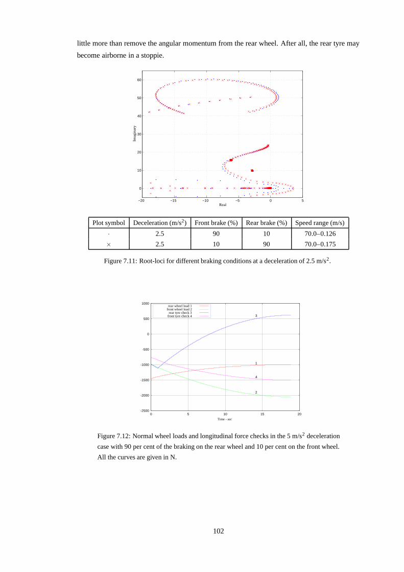
little more than remove the angular momentum from the rear wheel. After all, the rear tyre may
become airborne in a stoppie.
−20 −15 −10 −5 0 5
0
10
20
30
40
50
60
PSfrag replacements
Real
Imag
inar
y
Plot symbol Deceleration (m/s2) Front brake (%) Rear brake (%) Speed range (m/s)
· 2.5 90 10 70.0–0.126
× 2.5 10 90 70.0–0.175
Figure 7.11: Root-loci for different braking conditions at a deceleration of 2.5 m/s2.
-2500
-2000
-1500
-1000
-500
0
500
1000
0 5 10 15 20
3
1
4
2PSfrag replacements
Time - sec
rear wheel load 1front wheel load 2
rear tyre check 3front tyre check 4
Figure 7.12: Normal wheel loads and longitudinal force checks in the 5 m/s2 deceleration
case with 90 per cent of the braking on the rear wheel and 10 per cent on the front wheel.
All the curves are given in N.
102
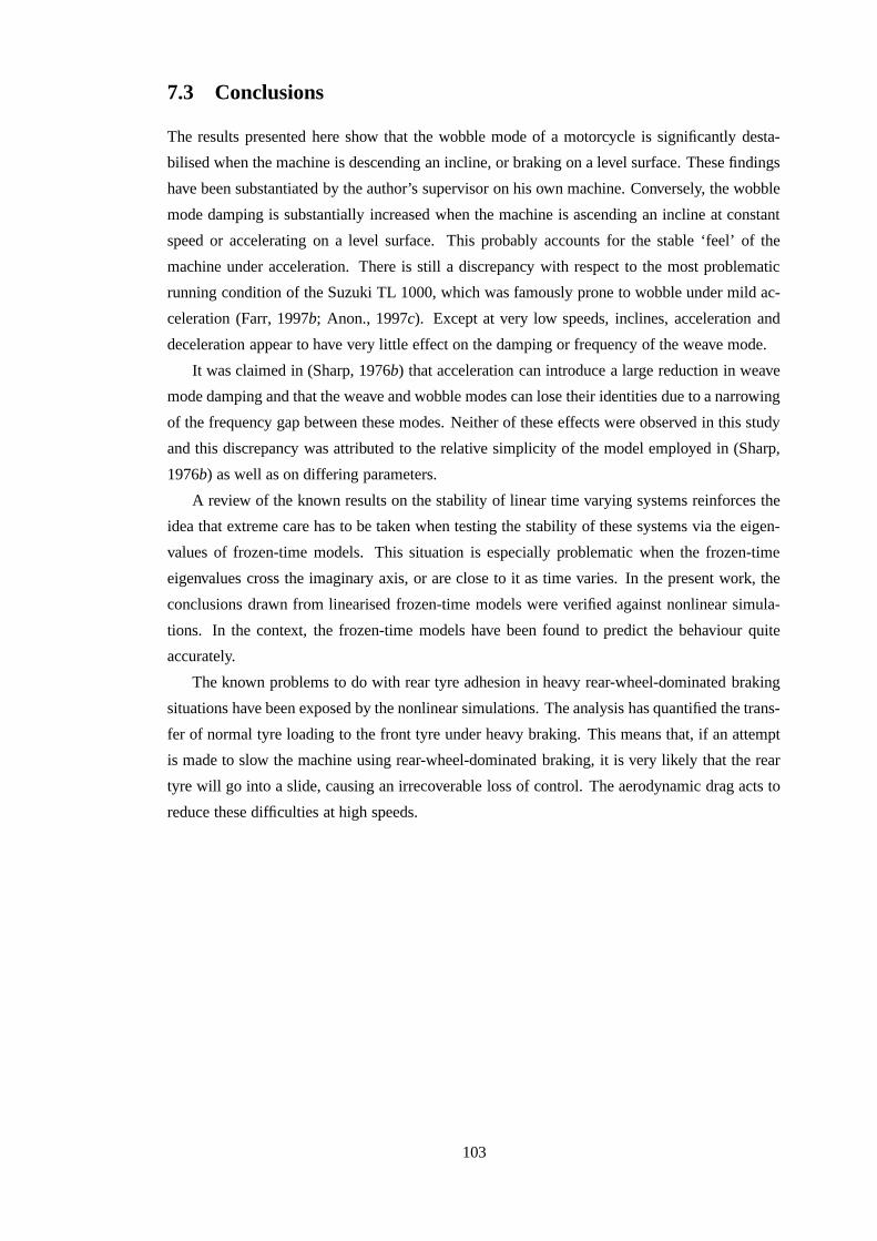
7.3 Conclusions
The results presented here show that the wobble mode of a motorcycle is significantly desta-
bilised when the machine is descending an incline, or braking on a level surface. These findings
have been substantiated by the author’s supervisor on his own machine. Conversely, the wobble
mode damping is substantially increased when the machine is ascending an incline at constant
speed or accelerating on a level surface. This probably accounts for the stable ‘feel’ of the
machine under acceleration. There is still a discrepancy with respect to the most problematic
running condition of the Suzuki TL 1000, which was famously prone to wobble under mild ac-
celeration (Farr, 1997b; Anon., 1997c). Except at very low speeds, inclines, acceleration and
deceleration appear to have very little effect on the damping or frequency of the weave mode.
It was claimed in (Sharp, 1976b) that acceleration can introduce a large reduction in weave
mode damping and that the weave and wobble modes can lose their identities due to a narrowing
of the frequency gap between these modes. Neither of these effects were observed in this study
and this discrepancy was attributed to the relative simplicity of the model employed in (Sharp,
1976b) as well as on differing parameters.
A review of the known results on the stability of linear time varying systems reinforces the
idea that extreme care has to be taken when testing the stability of these systems via the eigen-
values of frozen-time models. This situation is especially problematic when the frozen-time
eigenvalues cross the imaginary axis, or are close to it as time varies. In the present work, the
conclusions drawn from linearised frozen-time models were verified against nonlinear simula-
tions. In the context, the frozen-time models have been found to predict the behaviour quite
accurately.
The known problems to do with rear tyre adhesion in heavy rear-wheel-dominated braking
situations have been exposed by the nonlinear simulations. The analysis has quantified the trans-
fer of normal tyre loading to the front tyre under heavy braking. This means that, if an attempt
is made to slow the machine using rear-wheel-dominated braking, it is very likely that the rear
tyre will go into a slide, causing an irrecoverable loss of control. The aerodynamic drag acts to
reduce these difficulties at high speeds.
103
Chapter 8
Motorcycle steering oscillations due to
road profiling
8.1 Introduction
The previous chapter has shown that acceleration or deceleration can have an impact on the
stability of motorcycles. A source of even greater concern which can potentially endanger the
rider is the one described in this chapter. That is that there is a clear possibility for the lightly
damped modes of motorcycles to be excited by regular road surface undulations. The motivation
to study this issue is reinforced by a number of rider-loss-of-control incidents that have been
reported in the popular motorcycle press and involve no other road users. It is believed that road
forcing induced oscillations are strongly related to the causes of such accidents. These reports
are mainly non-technical and are based on anecdotal evidence, yet there is a compelling level of
consistency between them as we will see below.
One example of a loss-of-control event occurred during police motorcycle training and the
circumstances of this incident are summarised in the following extract from (Anon., 1993a):
“. . . there is a specific section of road which can cause severe handling difficulties for motorcy-
cles being ridden at high speed. . . this section of road has a series of small undulations in it at
the beginning of a large sweeping right hand bend. . . ”.
Another well-publicised event occurred at a relatively low speed under apparently benign
circumstances (Cutts, 1993): “. . . we were approaching a village at no more than 65/70 mph,
on a smooth road, on a constant or trailing throttle when, for no apparent reason, the bike went
wildly out of control. . . ”. This incident and some of the associated background are described
in (Evans, 1993; Raymond, 1993; Anon., 1993b,c).
A high profile fatal accident occurred, when according to an eye witness, the machine be-
ing ridden went into a violent “tank slapper”1 at about 60 mph as the rider was going around a
gentle corner (Duke, 1997). The offending machine model (Suzuki TL 1000) was subsequently
recalled in the U.S. (Anon., 1997c) as well as in the U.K. (Farr, 1997b). In their recall state-
1This expression is used to describe an oscillation that causes the handle bars to swing from lock to lock.
104
ment, the manufacturers said: “. . . the front wheel may oscillate, causing the handlebars to move
rapidly from side to side when accelerating from a corner and/or (accelerating) over a rough road
surface, commonly known as tank slapping. . . ”. There was further speculation as to the possible
causes of the difficulty and various tests were performed on the machine that involved changing
tyres, fitting a steering damper and changing the rear damper unit (Anon., 1997b). Tyre changes
did not seem to make a significant difference, but a steering damper and, strangely enough, a
new rear damper unit were reported to make a large improvement. One article claimed that riders
who weigh over 95 kg had not experienced the instability phenomena (Farr, 1997a).
A remarkable video tape of a weave-type instability was taken during the 1999 Formula One
Isle of Man TT race (Duke Marketing Ltd, 1999). Paul Orritt can be seen exiting the gentle
left-hand bend at the top of Bray Hill on a Honda Fireblade at approximately 150 mph when for
no apparent reason his machine went into an uncontrollable 2-3 Hz oscillation. His motorcycle
subsequently ran wide and crashed. “It just wouldn’t come out of the tank slapper,” he recalled.
“I was no longer in control . . . the trouble began immediately after I ran over a couple of bumps
in the freshly laid road surface. . . ” (Farrar, 2002). Another case of weave-type instability was
captured on video during the South African 250cc GP in April 2002. Casey Stoner can be
seen hitting a very small bump while exiting a corner, and subsequently undergoing an unstable
oscillation before falling on the road. His attempt to control the vehicle by using the brakes is
clear.
In technical terms, the mechanism by which an undulating road can influence the lateral
motions of a motorcycle is provided by the coupling terms between in-plane and out-of-plane
motions under cornering. A signal transmission path thus exists whereby steering oscillations
can be produced by road profiling. It is the author’s belief that the theory and results presented
here, provide an explanation for most of the behavioural problems described above.
In every case it will be assumed that the machine is operating in the neighbourhood of an
equilibrium cornering condition and the attention will be on quantifying the steering response
of the machine to regular road undulations through theoretical analysis. The associated design
parameter sensitivity problem is also studied. The machine condition of interest involves cor-
nering and consequently an elaborate mathematical model of the system is needed. The existing
state-of-the-art model in Chapter 5 is used with particular employment of the road forcing mech-
anism described there. The full nonlinear model is linearised for small perturbations about an
equilibrium cornering state that is found from a simulation of the motorcycle-rider system on a
smooth road. The linear, small perturbation, uncontrolled model is then subjected to sinusoidal
road displacement forcing and the frequency responses are computed. The responses to forcing
from both the front and rear wheels are considered. When studying the combined effects of
front and rear wheel road forcing, a wheelbase travel time delay is introduced into the model
that ensures that the two road wheel inputs are correctly phased.
105
8.1.1 Linearised models and Frequency response calculations
The preparation of linearised models involves a two-step procedure as usual. In the first, AU-
TOSIM is used to compute, symbolically, the linearised equations of motion. In the second, the
nonlinear simulation code is used to find the equilibrium state associated with the steady-state
cornering condition being studied, via the use of drive and steering controllers. The drive torque
is controlled so that the machine maintains a preset speed, while the steering torque is adjusted
to maintain a desired roll angle.
A number of Bode (frequency response) plots will be presented that were calculated using
the linearised models. In the current case, two inputs u f and ur are used. These represent
changes in the road height at the front and rear wheels’ ground contact points respectively. The
steering angle δ was the only output. Let us now suppose that the state-space model, generated
by AUTOSIM, that corresponds to a given cornering trim condition is:
x = Ax+Bu
δ = Cx
in which
u =
[
u f
ur
]
.
The transfer functions that relate the front and rear road disturbance input to the steering angle
are given by:[
g f gr
]
= C(sI −A)−1B
in which s is the usual Laplace transform complex variable. One can study separately the influ-
ences of the front and rear road-wheel disturbances using g f (s) and gr(s) independently. In the
case of studies of the combined influence of both wheels, the transfer function
g(s) = g f (s)+ e−sτgr(s)
is used, in which τ is the wheelbase filtering time delay given by wb/v. The constant wb is the
machine wheelbase and v its forward speed. All computations and plot outputs were computed
using MATLAB (The Mathworks Inc., 2000) M-files.
8.2 Results
8.2.1 Introductory comments
Straight running root-loci of the type presented in Figure 8.1 are well known from earlier chap-
ters.
This plot shows that the wobble mode is lightly damped at 13 m/s and that the associated
resonant frequency is approximately 48 rad/s (7.6 Hz). This diagram also shows that the weave
mode becomes lightly damped at high speeds and that the resonant frequency of this mode is ap-
proximately 22 rad/s (3.5 Hz) at a machine speed of 40 m/s. It should also be noted that the front
106
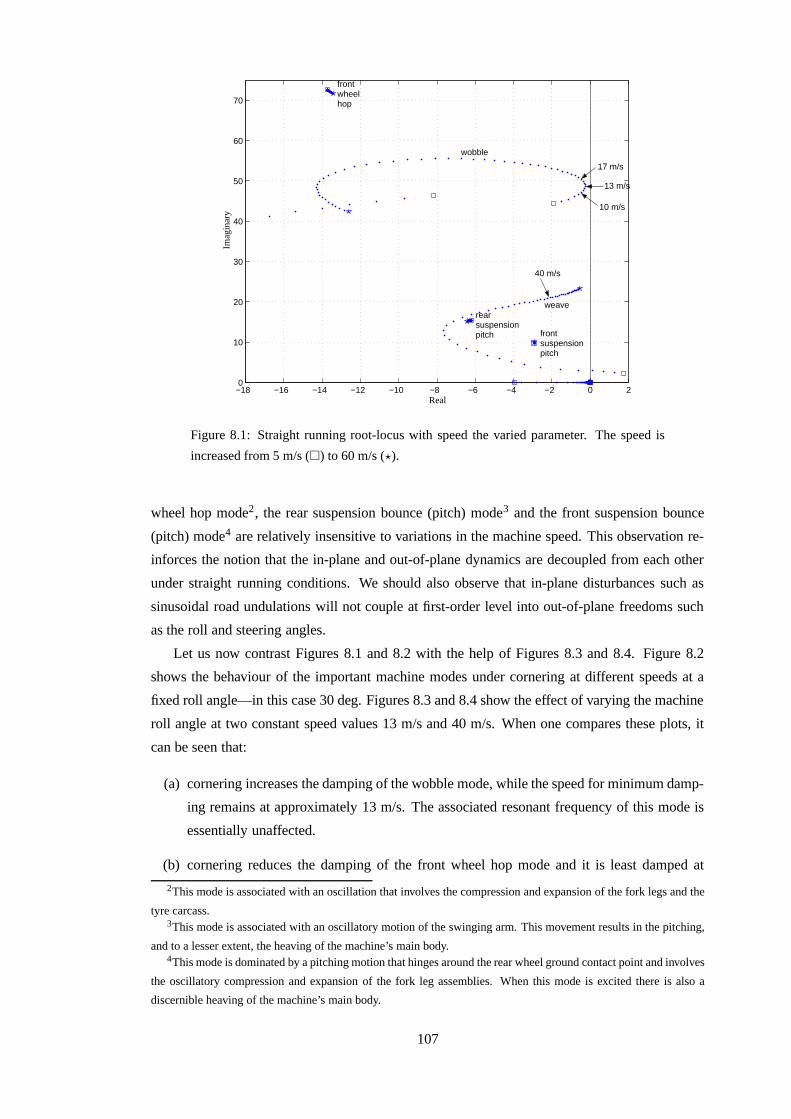
−18 −16 −14 −12 −10 −8 −6 −4 −2 0 20
10
20
30
40
50
60
70
10 m/s
13 m/s
17 m/s
wobble
weave
front suspensionpitch
rear suspensionpitch
40 m/s
frontwheelhop
PSfrag replacements
Imag
inar
y
Real
Figure 8.1: Straight running root-locus with speed the varied parameter. The speed is
increased from 5 m/s (�) to 60 m/s (?).
wheel hop mode2, the rear suspension bounce (pitch) mode3 and the front suspension bounce
(pitch) mode4 are relatively insensitive to variations in the machine speed. This observation re-
inforces the notion that the in-plane and out-of-plane dynamics are decoupled from each other
under straight running conditions. We should also observe that in-plane disturbances such as
sinusoidal road undulations will not couple at first-order level into out-of-plane freedoms such
as the roll and steering angles.
Let us now contrast Figures 8.1 and 8.2 with the help of Figures 8.3 and 8.4. Figure 8.2
shows the behaviour of the important machine modes under cornering at different speeds at a
fixed roll angle—in this case 30 deg. Figures 8.3 and 8.4 show the effect of varying the machine
roll angle at two constant speed values 13 m/s and 40 m/s. When one compares these plots, it
can be seen that:
(a) cornering increases the damping of the wobble mode, while the speed for minimum damp-
ing remains at approximately 13 m/s. The associated resonant frequency of this mode is
essentially unaffected.
(b) cornering reduces the damping of the front wheel hop mode and it is least damped at
2This mode is associated with an oscillation that involves the compression and expansion of the fork legs and the
tyre carcass.3This mode is associated with an oscillatory motion of the swinging arm. This movement results in the pitching,
and to a lesser extent, the heaving of the machine’s main body.4This mode is dominated by a pitching motion that hinges around the rear wheel ground contact point and involves
the oscillatory compression and expansion of the fork leg assemblies. When this mode is excited there is also a
discernible heaving of the machine’s main body.
107
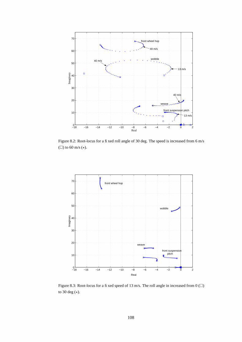
−18 −16 −14 −12 −10 −8 −6 −4 −2 0 20
10
20
30
40
50
60
70
wobble
front wheel hop
weave
front suspension pitch
40 m/s
40 m/s
13 m/s
40 m/s
13 m/s
PSfrag replacements
Imag
inar
y
Real
Figure 8.2: Root-locus for a fixed roll angle of 30 deg. The speed is increased from 6 m/s
(�) to 60 m/s (?).
−18 −16 −14 −12 −10 −8 −6 −4 −2 0 20
10
20
30
40
50
60
70
Real
Imag
inar
y
front wheel hop
wobble
weave
front suspension pitch
Figure 8.3: Root-locus for a fixed speed of 13 m/s. The roll angle in increased from 0 (�)
to 30 deg (?).
108

−18 −16 −14 −12 −10 −8 −6 −4 −2 0 20
10
20
30
40
50
60
70
Real
Imag
inar
y
front wheel hop
wobble
weave
front suspension pitch
Figure 8.4: Root-locus for a fixed speed of 40 m/s. The roll angle in increased from 0 (�)
to 30 deg (?).
approximately 40 m/s with an associated resonant frequency of approximately 63 rad/s
(10 Hz). This figure is lower than the straight running figure of 73 rad/s (11.6 Hz).
(c) cornering tends to reduce the damping of the weave mode and in the present case this
mode becomes unstable at high speed; the weave mode is lightly damped at 40 m/s.
(d) cornering has a destabilising effect on the front suspension pitch mode and it becomes
particularly lightly damped at 13 m/s and 30 deg of roll angle. The resonant frequency of
this mode is approximately 8 rad/s (1.27 Hz) under these conditions.
Since road forcing signals will couple into out-of-plane freedoms under cornering, these obser-
vations lead to the following hypotheses:
(a) The wobble and front suspension pitch modes are exposed to resonant forcing due to road
profiling at speeds of the order 13 m/s, and
(b) the weave and front wheel hop modes are similarly vulnerable at high speeds.
(c) Since the coupling between road disturbances and the out-of-plane dynamics increases
with roll angle, we expect to find an increase in the vulnerability of the front wheel hop
mode, the weave mode and the front suspension pitch mode with roll angle. All three
modal damping factors decrease with increasing roll angle.
(d) The vulnerability of the wobble mode is expected to reach a peak at some worst-case value
of roll angle. This is suggested because the interplane coupling increases with roll angle,
109
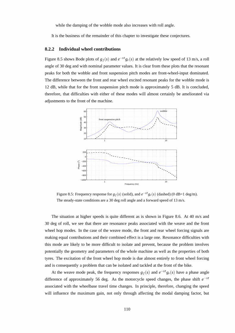
while the damping of the wobble mode also increases with roll angle.
It is the business of the remainder of this chapter to investigate these conjectures.
8.2.2 Individual wheel contributions
Figure 8.5 shows Bode plots of g f (s) and e−sτgr(s) at the relatively low speed of 13 m/s, a roll
angle of 30 deg and with nominal parameter values. It is clear from these plots that the resonant
peaks for both the wobble and front suspension pitch modes are front-wheel-input dominated.
The difference between the front and rear wheel excited resonant peaks for the wobble mode is
12 dB, while that for the front suspension pitch mode is approximately 5 dB. It is concluded,
therefore, that difficulties with either of these modes will almost certainly be ameliorated via
adjustments to the front of the machine.
1 1010
20
30
40
50
60
Mag
nitu
de (
dB)
1 10−1000
−800
−600
−400
−200
0
200
Frequency (Hz)
Pha
se (
o )
PSfrag replacements
wobble
front suspension pitch
Figure 8.5: Frequency response for g f (s) (solid), and e−sτgr(s) (dashed) (0 dB=1 deg/m).
The steady-state conditions are a 30 deg roll angle and a forward speed of 13 m/s.
The situation at higher speeds is quite different as is shown in Figure 8.6. At 40 m/s and
30 deg of roll, we see that there are resonance peaks associated with the weave and the front
wheel hop modes. In the case of the weave mode, the front and rear wheel forcing signals are
making equal contributions and their combined effect is a large one. Resonance difficulties with
this mode are likely to be more difficult to isolate and prevent, because the problem involves
potentially the geometry and parameters of the whole machine as well as the properties of both
tyres. The excitation of the front wheel hop mode is due almost entirely to front wheel forcing
and is consequently a problem that can be isolated and tackled at the front of the bike.
At the weave mode peak, the frequency responses g f (s) and e−sτ gr(s) have a phase angle
difference of approximately 56 deg. As the motorcycle speed changes, the phase shift e−sτ
associated with the wheelbase travel time changes. In principle, therefore, changing the speed
will influence the maximum gain, not only through affecting the modal damping factor, but
110
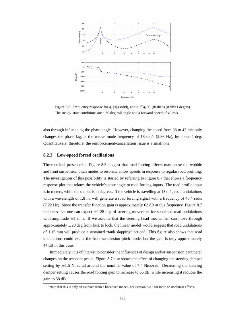
2 3 4 5 6 7 8 9 1010
20
30
40
50
60
Mag
nitu
de (
dB)
2 3 4 5 6 7 8 9 10−1000
−800
−600
−400
−200
0
200
Frequency (Hz)
Pha
se (
o )
PSfrag replacements
wea
ve
front wheel hop
Figure 8.6: Frequency response for g f (s) (solid), and e−sτgr(s) (dashed) (0 dB=1 deg/m).
The steady-state conditions are a 30 deg roll angle and a forward speed of 40 m/s.
also through influencing the phase angle. However, changing the speed from 38 to 42 m/s only
changes the phase lag, at the weave mode frequency of 18 rad/s (2.86 Hz), by about 4 deg.
Quantitatively, therefore, the reinforcement/cancellation issue is a small one.
8.2.3 Low-speed forced oscillations
The root-loci presented in Figure 8.3 suggest that road forcing effects may cause the wobble
and front suspension pitch modes to resonate at low speeds in response to regular road profiling.
The investigation of this possibility is started by referring to Figure 8.7 that shows a frequency
response plot that relates the vehicle’s steer angle to road forcing inputs. The road profile input
is in meters, while the output is in degrees. If the vehicle is travelling at 13 m/s, road undulations
with a wavelength of 1.8 m, will generate a road forcing signal with a frequency of 45.4 rad/s
(7.22 Hz). Since the transfer function gain is approximately 62 dB at this frequency, Figure 8.7
indicates that one can expect ±1.28 deg of steering movement for sustained road undulations
with amplitude ±1 mm. If we assume that the steering head mechanism can move through
approximately ±20 deg from lock to lock, the linear model would suggest that road undulations
of ±15 mm will produce a sustained “tank slapping” action5 . This figure also shows that road
undulations could excite the front suspension pitch mode, but the gain is only approximately
44 dB in this case.
Immediately, it is of interest to consider the influences of design and/or suspension parameter
changes on the resonant peaks. Figure 8.7 also shows the effect of changing the steering damper
setting by ±1.5 Nms/rad around the nominal value of 7.4 Nms/rad. Decreasing the steering
damper setting causes the road forcing gain to increase to 66 dB, while increasing it reduces the
gain to 58 dB.
5Note that this is only an estimate from a linearised model—see Section 8.2.6 for more on nonlinear effects.
111
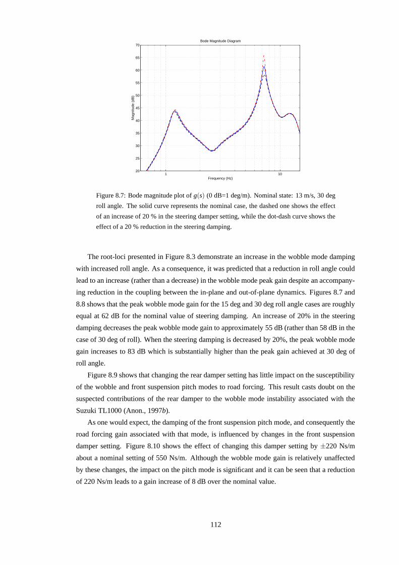
1 1020
25
30
35
40
45
50
55
60
65
70
Frequency (Hz)
Mag
nitu
de (
dB)
Bode Magnitude Diagram
Figure 8.7: Bode magnitude plot of g(s) (0 dB=1 deg/m). Nominal state: 13 m/s, 30 deg
roll angle. The solid curve represents the nominal case, the dashed one shows the effect
of an increase of 20 % in the steering damper setting, while the dot-dash curve shows the
effect of a 20 % reduction in the steering damping.
The root-loci presented in Figure 8.3 demonstrate an increase in the wobble mode damping
with increased roll angle. As a consequence, it was predicted that a reduction in roll angle could
lead to an increase (rather than a decrease) in the wobble mode peak gain despite an accompany-
ing reduction in the coupling between the in-plane and out-of-plane dynamics. Figures 8.7 and
8.8 shows that the peak wobble mode gain for the 15 deg and 30 deg roll angle cases are roughly
equal at 62 dB for the nominal value of steering damping. An increase of 20% in the steering
damping decreases the peak wobble mode gain to approximately 55 dB (rather than 58 dB in the
case of 30 deg of roll). When the steering damping is decreased by 20%, the peak wobble mode
gain increases to 83 dB which is substantially higher than the peak gain achieved at 30 deg of
roll angle.
Figure 8.9 shows that changing the rear damper setting has little impact on the susceptibility
of the wobble and front suspension pitch modes to road forcing. This result casts doubt on the
suspected contributions of the rear damper to the wobble mode instability associated with the
Suzuki TL1000 (Anon., 1997b).
As one would expect, the damping of the front suspension pitch mode, and consequently the
road forcing gain associated with that mode, is influenced by changes in the front suspension
damper setting. Figure 8.10 shows the effect of changing this damper setting by ±220 Ns/m
about a nominal setting of 550 Ns/m. Although the wobble mode gain is relatively unaffected
by these changes, the impact on the pitch mode is significant and it can be seen that a reduction
of 220 Ns/m leads to a gain increase of 8 dB over the nominal value.
112
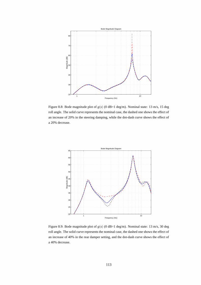
1 1020
30
40
50
60
70
80
Frequency (Hz)
Mag
nitu
de (
dB)
Bode Magnitude Diagram
Figure 8.8: Bode magnitude plot of g(s) (0 dB=1 deg/m). Nominal state: 13 m/s, 15 deg
roll angle. The solid curve represents the nominal case, the dashed one shows the effect of
an increase of 20% in the steering damping, while the dot-dash curve shows the effect of
a 20% decrease.
1 1020
25
30
35
40
45
50
55
60
65
Frequency (Hz)
Mag
nitu
de (
dB)
Bode Magnitude Diagram
Figure 8.9: Bode magnitude plot of g(s) (0 dB=1 deg/m). Nominal state: 13 m/s, 30 deg
roll angle. The solid curve represents the nominal case, the dashed one shows the effect of
an increase of 40% in the rear damper setting, and the dot-dash curve shows the effect of
a 40% decrease.
113
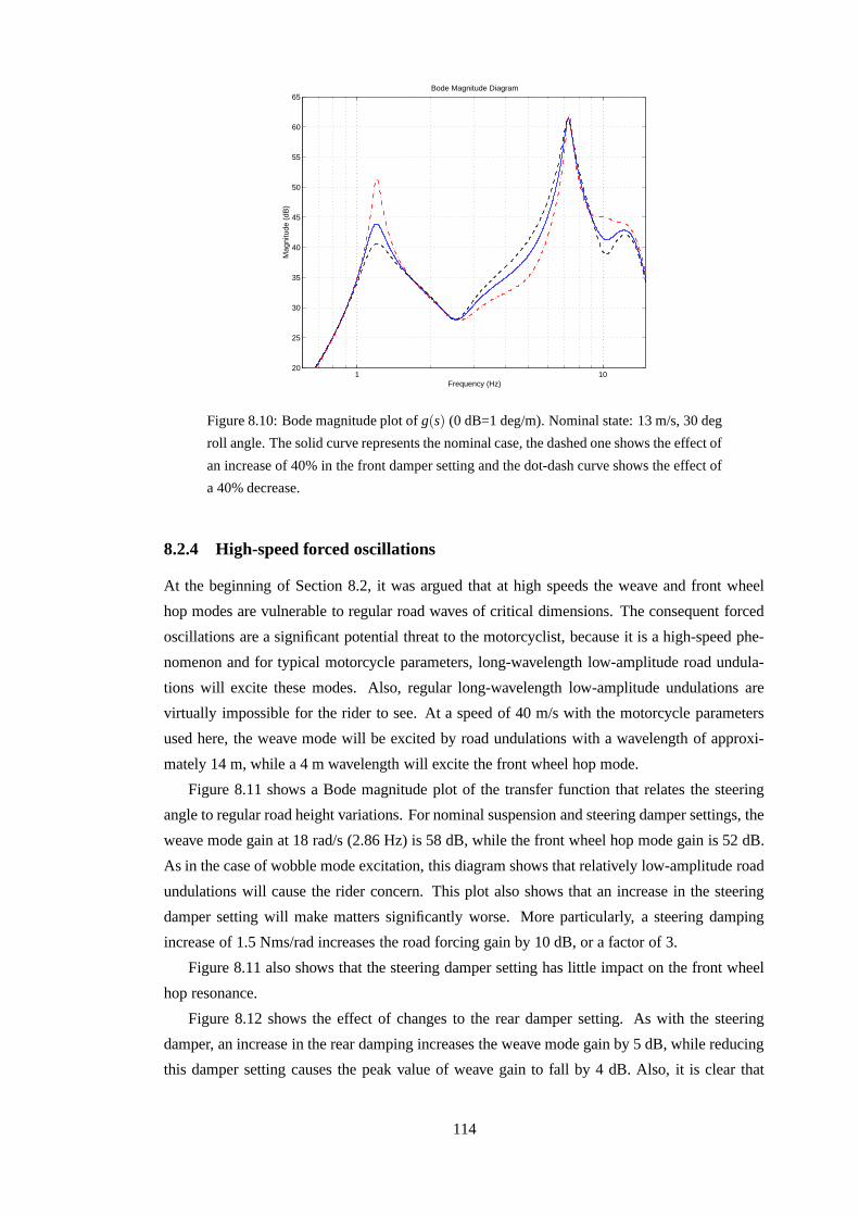
1 1020
25
30
35
40
45
50
55
60
65
Frequency (Hz)
Mag
nitu
de (
dB)
Bode Magnitude Diagram
Figure 8.10: Bode magnitude plot of g(s) (0 dB=1 deg/m). Nominal state: 13 m/s, 30 deg
roll angle. The solid curve represents the nominal case, the dashed one shows the effect of
an increase of 40% in the front damper setting and the dot-dash curve shows the effect of
a 40% decrease.
8.2.4 High-speed forced oscillations
At the beginning of Section 8.2, it was argued that at high speeds the weave and front wheel
hop modes are vulnerable to regular road waves of critical dimensions. The consequent forced
oscillations are a significant potential threat to the motorcyclist, because it is a high-speed phe-
nomenon and for typical motorcycle parameters, long-wavelength low-amplitude road undula-
tions will excite these modes. Also, regular long-wavelength low-amplitude undulations are
virtually impossible for the rider to see. At a speed of 40 m/s with the motorcycle parameters
used here, the weave mode will be excited by road undulations with a wavelength of approxi-
mately 14 m, while a 4 m wavelength will excite the front wheel hop mode.
Figure 8.11 shows a Bode magnitude plot of the transfer function that relates the steering
angle to regular road height variations. For nominal suspension and steering damper settings, the
weave mode gain at 18 rad/s (2.86 Hz) is 58 dB, while the front wheel hop mode gain is 52 dB.
As in the case of wobble mode excitation, this diagram shows that relatively low-amplitude road
undulations will cause the rider concern. This plot also shows that an increase in the steering
damper setting will make matters significantly worse. More particularly, a steering damping
increase of 1.5 Nms/rad increases the road forcing gain by 10 dB, or a factor of 3.
Figure 8.11 also shows that the steering damper setting has little impact on the front wheel
hop resonance.
Figure 8.12 shows the effect of changes to the rear damper setting. As with the steering
damper, an increase in the rear damping increases the weave mode gain by 5 dB, while reducing
this damper setting causes the peak value of weave gain to fall by 4 dB. Also, it is clear that
114
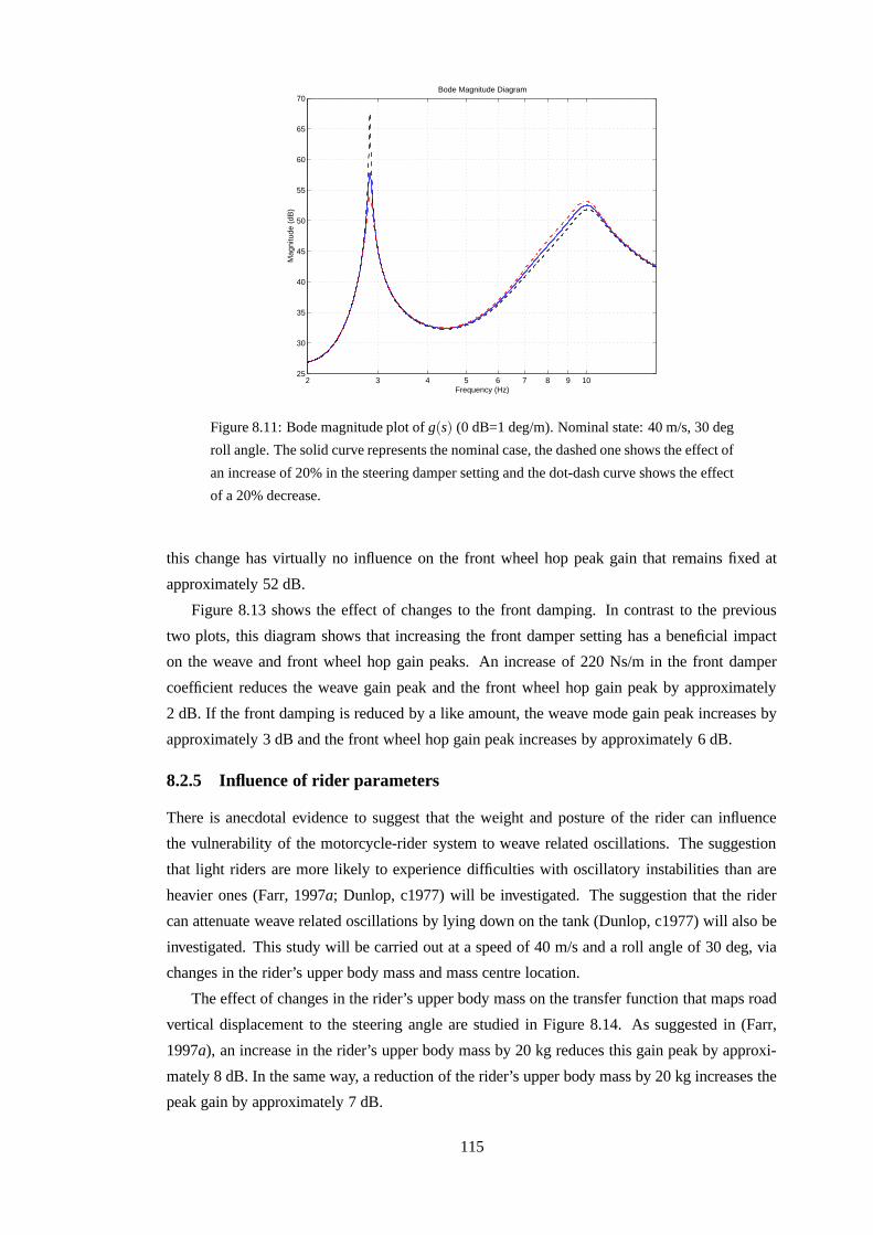
2 3 4 5 6 7 8 9 1025
30
35
40
45
50
55
60
65
70
Frequency (Hz)
Mag
nitu
de (
dB)
Bode Magnitude Diagram
Figure 8.11: Bode magnitude plot of g(s) (0 dB=1 deg/m). Nominal state: 40 m/s, 30 deg
roll angle. The solid curve represents the nominal case, the dashed one shows the effect of
an increase of 20% in the steering damper setting and the dot-dash curve shows the effect
of a 20% decrease.
this change has virtually no influence on the front wheel hop peak gain that remains fixed at
approximately 52 dB.
Figure 8.13 shows the effect of changes to the front damping. In contrast to the previous
two plots, this diagram shows that increasing the front damper setting has a beneficial impact
on the weave and front wheel hop gain peaks. An increase of 220 Ns/m in the front damper
coefficient reduces the weave gain peak and the front wheel hop gain peak by approximately
2 dB. If the front damping is reduced by a like amount, the weave mode gain peak increases by
approximately 3 dB and the front wheel hop gain peak increases by approximately 6 dB.
8.2.5 Influence of rider parameters
There is anecdotal evidence to suggest that the weight and posture of the rider can influence
the vulnerability of the motorcycle-rider system to weave related oscillations. The suggestion
that light riders are more likely to experience difficulties with oscillatory instabilities than are
heavier ones (Farr, 1997a; Dunlop, c1977) will be investigated. The suggestion that the rider
can attenuate weave related oscillations by lying down on the tank (Dunlop, c1977) will also be
investigated. This study will be carried out at a speed of 40 m/s and a roll angle of 30 deg, via
changes in the rider’s upper body mass and mass centre location.
The effect of changes in the rider’s upper body mass on the transfer function that maps road
vertical displacement to the steering angle are studied in Figure 8.14. As suggested in (Farr,
1997a), an increase in the rider’s upper body mass by 20 kg reduces this gain peak by approxi-
mately 8 dB. In the same way, a reduction of the rider’s upper body mass by 20 kg increases the
peak gain by approximately 7 dB.
115
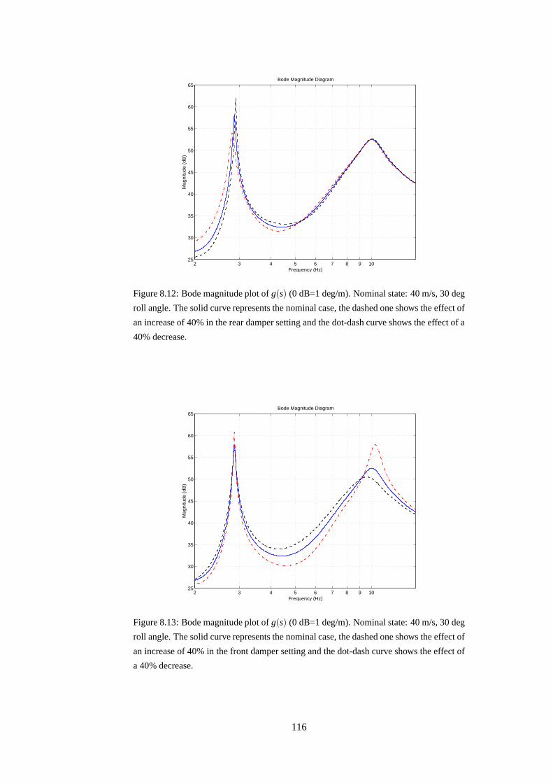
2 3 4 5 6 7 8 9 1025
30
35
40
45
50
55
60
65
Frequency (Hz)
Mag
nitu
de (
dB)
Bode Magnitude Diagram
Figure 8.12: Bode magnitude plot of g(s) (0 dB=1 deg/m). Nominal state: 40 m/s, 30 deg
roll angle. The solid curve represents the nominal case, the dashed one shows the effect of
an increase of 40% in the rear damper setting and the dot-dash curve shows the effect of a
40% decrease.
2 3 4 5 6 7 8 9 1025
30
35
40
45
50
55
60
65
Frequency (Hz)
Mag
nitu
de (
dB)
Bode Magnitude Diagram
Figure 8.13: Bode magnitude plot of g(s) (0 dB=1 deg/m). Nominal state: 40 m/s, 30 deg
roll angle. The solid curve represents the nominal case, the dashed one shows the effect of
an increase of 40% in the front damper setting and the dot-dash curve shows the effect of
a 40% decrease.
116
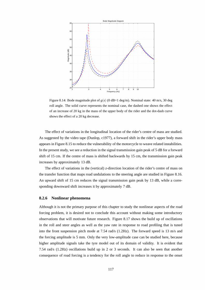
2 3 4 5 6 7 8 9 1025
30
35
40
45
50
55
60
65
Frequency (Hz)
Mag
nitu
de (
dB)
Bode Magnitude Diagram
Figure 8.14: Bode magnitude plot of g(s) (0 dB=1 deg/m). Nominal state: 40 m/s, 30 deg
roll angle. The solid curve represents the nominal case, the dashed one shows the effect
of an increase of 20 kg in the mass of the upper body of the rider and the dot-dash curve
shows the effect of a 20 kg decrease.
The effect of variations in the longitudinal location of the rider’s centre of mass are studied.
As suggested by the video tape (Dunlop, c1977), a forward shift in the rider’s upper body mass
appears in Figure 8.15 to reduce the vulnerability of the motorcycle to weave related instabilities.
In the present study, we see a reduction in the signal transmission gain peak of 5 dB for a forward
shift of 15 cm. If the centre of mass is shifted backwards by 15 cm, the transmission gain peak
increases by approximately 13 dB.
The effect of variations in the (vertical) z-direction location of the rider’s centre of mass on
the transfer function that maps road undulations to the steering angle are studied in Figure 8.16.
An upward shift of 15 cm reduces the signal transmission gain peak by 13 dB, while a corre-
sponding downward shift increases it by approximately 7 dB.
8.2.6 Nonlinear phenomena
Although it is not the primary purpose of this chapter to study the nonlinear aspects of the road
forcing problem, it is desired not to conclude this account without making some introductory
observations that will motivate future research. Figure 8.17 shows the build up of oscillations
in the roll and steer angles as well as the yaw rate in response to road profiling that is tuned
into the front suspension pitch mode at 7.54 rad/s (1.2Hz). The forward speed is 13 m/s and
the forcing amplitude is 5 mm. Only the very low-amplitude case can be studied here, because
higher amplitude signals take the tyre model out of its domain of validity. It is evident that
7.54 rad/s (1.2Hz) oscillations build up in 2 or 3 seconds. It can also be seen that another
consequence of road forcing is a tendency for the roll angle to reduce in response to the onset
117
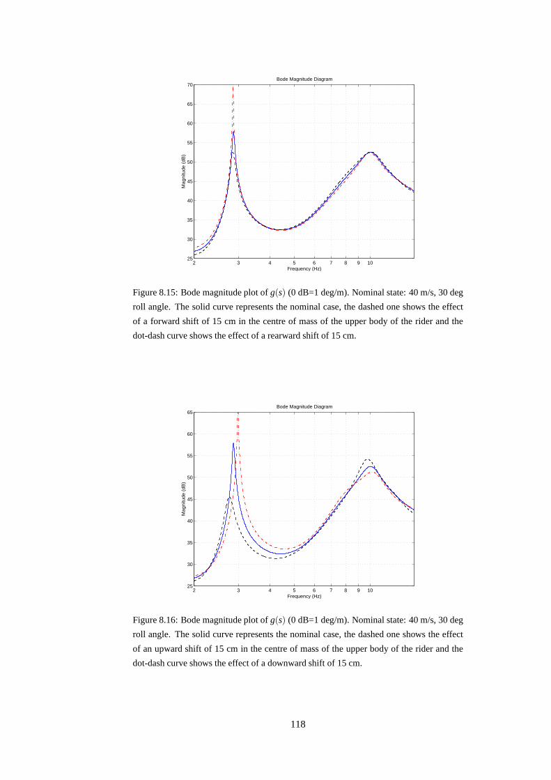
2 3 4 5 6 7 8 9 1025
30
35
40
45
50
55
60
65
70
Frequency (Hz)
Mag
nitu
de (
dB)
Bode Magnitude Diagram
Figure 8.15: Bode magnitude plot of g(s) (0 dB=1 deg/m). Nominal state: 40 m/s, 30 deg
roll angle. The solid curve represents the nominal case, the dashed one shows the effect
of a forward shift of 15 cm in the centre of mass of the upper body of the rider and the
dot-dash curve shows the effect of a rearward shift of 15 cm.
2 3 4 5 6 7 8 9 1025
30
35
40
45
50
55
60
65
Frequency (Hz)
Mag
nitu
de (
dB)
Bode Magnitude Diagram
Figure 8.16: Bode magnitude plot of g(s) (0 dB=1 deg/m). Nominal state: 40 m/s, 30 deg
roll angle. The solid curve represents the nominal case, the dashed one shows the effect
of an upward shift of 15 cm in the centre of mass of the upper body of the rider and the
dot-dash curve shows the effect of a downward shift of 15 cm.
118
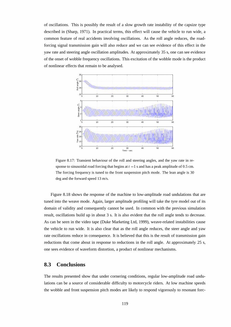
of oscillations. This is possibly the result of a slow growth rate instability of the capsize type
described in (Sharp, 1971). In practical terms, this effect will cause the vehicle to run wide, a
common feature of real accidents involving oscillations. As the roll angle reduces, the road-
forcing signal transmission gain will also reduce and we can see evidence of this effect in the
yaw rate and steering angle oscillation amplitudes. At approximately 35 s, one can see evidence
of the onset of wobble frequency oscillations. This excitation of the wobble mode is the product
of nonlinear effects that remain to be analysed.
0 10 20 30 40 50 6020
25
30
35R
oll a
ngle
(o )
0 10 20 30 40 50 601
2
3
4
Ste
er a
ngle
(o )
0 10 20 30 40 50 6010
15
20
25
30
Time − sec
Yaw
rat
e (o /s
)
Figure 8.17: Transient behaviour of the roll and steering angles, and the yaw rate in re-
sponse to sinusoidal road forcing that begins at t =1 s and has a peak amplitude of 0.5 cm.
The forcing frequency is tuned to the front suspension pitch mode. The lean angle is 30
deg and the forward speed 13 m/s.
Figure 8.18 shows the response of the machine to low-amplitude road undulations that are
tuned into the weave mode. Again, larger amplitude profiling will take the tyre model out of its
domain of validity and consequently cannot be used. In common with the previous simulation
result, oscillations build up in about 3 s. It is also evident that the roll angle tends to decrease.
As can be seen in the video tape (Duke Marketing Ltd, 1999), weave-related instabilities cause
the vehicle to run wide. It is also clear that as the roll angle reduces, the steer angle and yaw
rate oscillations reduce in consequence. It is believed that this is the result of transmission gain
reductions that come about in response to reductions in the roll angle. At approximately 25 s,
one sees evidence of waveform distortion, a product of nonlinear mechanisms.
8.3 Conclusions
The results presented show that under cornering conditions, regular low-amplitude road undu-
lations can be a source of considerable difficulty to motorcycle riders. At low machine speeds
the wobble and front suspension pitch modes are likely to respond vigorously to resonant forc-
119
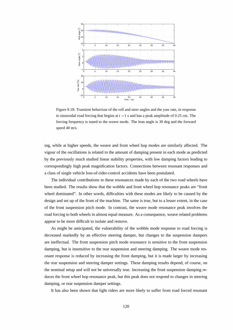
0 5 10 15 20 25 30 35 4020
25
30
35
Rol
l ang
le (
o )
0 5 10 15 20 25 30 35 40−1
0
1
2
Ste
er a
ngle
(o )
0 5 10 15 20 25 30 35 40−20
0
20
40
Time − sec
Yaw
rat
e (o /s
)
Figure 8.18: Transient behaviour of the roll and steer angles and the yaw rate, in response
to sinusoidal road forcing that begins at t =1 s and has a peak amplitude of 0.25 cm. The
forcing frequency is tuned to the weave mode. The lean angle is 30 deg and the forward
speed 40 m/s.
ing, while at higher speeds, the weave and front wheel hop modes are similarly affected. The
vigour of the oscillations is related to the amount of damping present in each mode as predicted
by the previously much studied linear stability properties, with low damping factors leading to
correspondingly high peak magnification factors. Connections between resonant responses and
a class of single vehicle loss-of-rider-control accidents have been postulated.
The individual contributions to these resonances made by each of the two road wheels have
been studied. The results show that the wobble and front wheel hop resonance peaks are “front
wheel dominated”. In other words, difficulties with these modes are likely to be caused by the
design and set up of the front of the machine. The same is true, but to a lesser extent, in the case
of the front suspension pitch mode. In contrast, the weave mode resonance peak involves the
road forcing to both wheels in almost equal measure. As a consequence, weave related problems
appear to be more difficult to isolate and remove.
As might be anticipated, the vulnerability of the wobble mode response to road forcing is
decreased markedly by an effective steering damper, but changes to the suspension dampers
are ineffectual. The front suspension pitch mode resonance is sensitive to the front suspension
damping, but is insensitive to the rear suspension and steering damping. The weave mode res-
onant response is reduced by increasing the front damping, but it is made larger by increasing
the rear suspension and steering damper settings. These damping results depend, of course, on
the nominal setup and will not be universally true. Increasing the front suspension damping re-
duces the front wheel hop resonance peak, but this peak does not respond to changes in steering
damping, or rear suspension damper settings.
It has also been shown that light riders are more likely to suffer from road forced resonant
120
weave oscillations than are heavy ones, as has been observed in practice (Farr, 1997a) and on
the video tape (Dunlop, c1977). The results indicate also that the peak gains associated with
the weave mode are brought down by moving the rider upper body mass forwards and upwards.
There is not sufficient practical evidence at the moment to indicate whether or not these findings
coincide with experience. From the rider’s perspective, a worrying feature of the road profile
induced oscillations is the tendency of the uncontrolled machine to “sit up” and run wide. This
aspect of the machine behaviour can be seen on the video tape (Duke Marketing Ltd, 1999) in
the case of a high-speed weave accident.
A preliminary study of motion simulations under resonance conditions has shown the exis-
tence of interesting and essentially nonlinear phenomena, that seem to conform with practical
experience. These nonlinear phenomena are worthy of further study.
121
Part IV
Modelling Upgrades
122
Chapter 9
An improved motorcycle model
This chapter deals with recent work in bringing the already advanced model of Chapter 5 in line
with modern motorcycle designs, both at the conceptual level and the parametric description.
Some of the work presented here was also covered in (Sharp et al., 2003).
In the base configuration the upgraded model has the same number of bodies and freedoms
as the one in Chapter 5. The addition of new bodies will be required for some of the new configu-
rations considered below, such as the chain drive system and telelever front suspension. The new
monoshock rear suspension does not require any further bodies. It is possible to switch among
the various configurations by activating the appropriate Lisp logical variables at the beginning
of the AUTOSIM code to allow the Lisp macros ������ ��� and � � � � to choose the relevant pieces
of code from the master file. A similar method was described earlier in Chapters 3 and 4 in the
context of choosing between the nonlinear and linearised models, except that this time there are
many more flags.
9.1 Parametric description
A measurement campaign to obtain the relevant parameter values of a Suzuki GSX-R1000 mo-
torcycle is currently in progress. One such machine has been disassembled and many parameters
of the parts have been measured. At this point the campaign is incomplete and the measurements
that are pending will be pointed out below together with those already done. This machine comes
with a monoshock rear suspension, and the associated parameters with this type of suspension
can be measured. For the front suspension the only parameters possible to obtain are those for
the telescopic forks that come with this machine, and parameters for a telelever type suspension
should be pursued elsewhere.
9.1.1 Geometry, mass centres, masses and inertias
The workshop manual for the motorcycle includes pictures to scale and key dimensions, like
the wheelbase and the steering head angle. Joints between components at the steering head
and the swing arm pivot can be identified there and many key points, including those related to
123
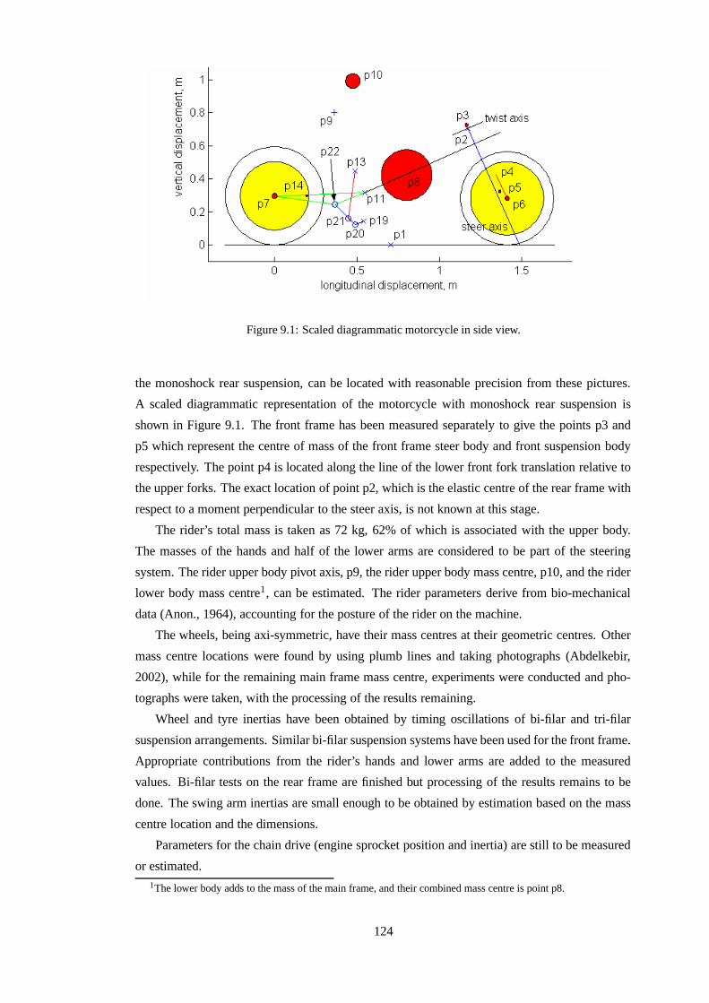
Figure 9.1: Scaled diagrammatic motorcycle in side view.
the monoshock rear suspension, can be located with reasonable precision from these pictures.
A scaled diagrammatic representation of the motorcycle with monoshock rear suspension is
shown in Figure 9.1. The front frame has been measured separately to give the points p3 and
p5 which represent the centre of mass of the front frame steer body and front suspension body
respectively. The point p4 is located along the line of the lower front fork translation relative to
the upper forks. The exact location of point p2, which is the elastic centre of the rear frame with
respect to a moment perpendicular to the steer axis, is not known at this stage.
The rider’s total mass is taken as 72 kg, 62% of which is associated with the upper body.
The masses of the hands and half of the lower arms are considered to be part of the steering
system. The rider upper body pivot axis, p9, the rider upper body mass centre, p10, and the rider
lower body mass centre1, can be estimated. The rider parameters derive from bio-mechanical
data (Anon., 1964), accounting for the posture of the rider on the machine.
The wheels, being axi-symmetric, have their mass centres at their geometric centres. Other
mass centre locations were found by using plumb lines and taking photographs (Abdelkebir,
2002), while for the remaining main frame mass centre, experiments were conducted and pho-
tographs were taken, with the processing of the results remaining.
Wheel and tyre inertias have been obtained by timing oscillations of bi-filar and tri-filar
suspension arrangements. Similar bi-filar suspension systems have been used for the front frame.
Appropriate contributions from the rider’s hands and lower arms are added to the measured
values. Bi-filar tests on the rear frame are finished but processing of the results remains to be
done. The swing arm inertias are small enough to be obtained by estimation based on the mass
centre location and the dimensions.
Parameters for the chain drive (engine sprocket position and inertia) are still to be measured
or estimated.1The lower body adds to the mass of the main frame, and their combined mass centre is point p8.
124
9.1.2 Stiffness and damping properties
Springs and damper units were tested in a standard dynamic materials testing machine (Ab-
delkebir, 2002). The damper characteristic measurements were limited by the maximum actu-
ator velocity available of about 0.25 m/s. Uni-directional forcing of the steering damper at the
maximum rate of the actuator yielded a substantially linear force / velocity relationship with
slope 4340 N/(m/s). Using the effective moment arm of the damper (0.04 m) this value was
converted to an equivalent rotational coefficient of value 6.944 Nm/(rad/s).
The dimensions of the single steel spring from the monoshock rear suspension were mea-
sured, and the standard helical spring formula, k = Gd4/(64R3n), was applied to calculating the
rate, k, as 55000 N/m. The gas filled damper contributes some suspension preload and a small
rate which was determined from the test machine via static measurements as 3570 N/m. The
damper unit was stroked at full actuator performance first in compression and then in extension,
achieving velocities up to about 0.13 m/s. Allowing for the gas pressure forces in the processing,
the damping coefficient in compression was 9600 N/(m/s) and in rebound 13700 N/(m/s). Front
spring and damper coefficients need to be measured. Suspension limit stops are included at each
end, modelled as fifth powers of displacement from stop contact. The relevant displacements are
known from examination of the parts and from information given in the workshop manual.
The torsional stiffness of the main frame, between the steering head and the power unit, is
yet to be measured. It is clear from the structural design and materials used that the frame is
considerably stiffer than conventional tubular framed motorcycles of some years ago. In those
cases, it was established that the frame flexibility was an essential contributor to the stability
of the wobble mode, in particular (Sharp and Alstead, 1980; Spierings, 1981). It remains to
be seen how significant this area is for modern machines. Tyre radial stiffnesses come directly
from (Cossalter and Lot, 2002).
The rider’s upper body has roll freedom relative to the main frame, while the lower body is
part of the main frame. The upper body is restrained by a parallel spring damper system, stiff
enough to give a decoupled natural frequency of 11.7 Hz for the rider upper body lean motion.
This allows only a modest participation of the rider body in the motorcycle motions.
9.1.3 Aerodynamics
In-plane aerodynamic effects are included, and associated aerodynamic force and moment data
comes from a Triumph motorcycle of similar style and dimensions to the GSX-R1000 (Sharp,
2001). This is steady-state drag force, lift force and pitching moment data from full scale wind
tunnel testing, with a prone rider.
9.2 Tyre-road contact modelling
A correct representation of the tyre-road contact is important in the accuracy of predicted be-
haviour for the motorcycle. The geometries involved are naturally complex, especially at the
125
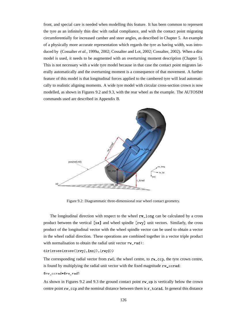
front, and special care is needed when modelling this feature. It has been common to represent
the tyre as an infinitely thin disc with radial compliance, and with the contact point migrating
circumferentially for increased camber and steer angles, as described in Chapter 5. An example
of a physically more accurate representation which regards the tyre as having width, was intro-
duced by (Cossalter et al., 1999a, 2002; Cossalter and Lot, 2002; Cossalter, 2002). When a disc
model is used, it needs to be augmented with an overturning moment description (Chapter 5).
This is not necessary with a wide tyre model because in that case the contact point migrates lat-
erally automatically and the overturning moment is a consequence of that movement. A further
feature of this model is that longitudinal forces applied to the cambered tyre will lead automati-
cally to realistic aligning moments. A wide tyre model with circular cross-section crown is now
modelled, as shown in Figures 9.2 and 9.3, with the rear wheel as the example. The AUTOSIM
commands used are described in Appendix B.
���������������������������������������������������������������������������������������������������������������������������������������������������������������������������������������������������������������������������������������������������������������������
���������������������������������������������������������������������������������������������������������������������������������������������������������������������������������������������������������������������������������������������������������������
r_tcrad
rw_c
crad
rw_long
rw_lat
[nz]
rw_long
n0
pos(rw0,n0)
rw0
rw_cp
rw_ccp
Figure 9.2: Diagrammatic three-dimensional rear wheel contact geometry.
The longitudinal direction with respect to the wheel � � � � F � ? can be calculated by a cross
product between the vertical�� ��� and wheel spindle
�� � A�� unit vectors. Similarly, the cross
product of the longitudinal vector with the wheel spindle vector can be used to obtain a vector
in the wheel radial direction. These operations are combined together in a vector triple product
with normalisation to obtain the radial unit vector � � � � � :���, ��;'�+����-��;'�+����-��� 6�! � ��� �(� ��� ��� 6�! ����
The corresponding radial vector from � � � , the wheel centre, to � � � H�H G , the tyre crown centre,
is found by multiplying the radial unit vector with the fixed magnitude � � � H�H � :��6�2�;�;'����� ��6�2�����
As shown in Figures 9.2 and 9.3 the ground contact point � � � H G is vertically below the crown
centre point � � � H�H G and the nominal distance between them is � � � H � . In general this distance
126
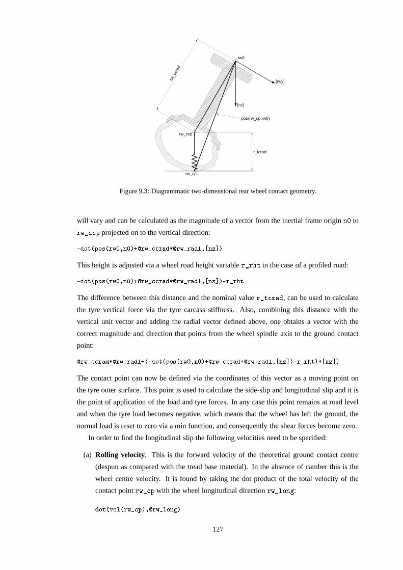
rw_c
crad
[rwy]
[nz]
r_tcrad
rw_ccp
rw0
rw_cp
pos(rw_cp,rw0)
Figure 9.3: Diagrammatic two-dimensional rear wheel contact geometry.
will vary and can be calculated as the magnitude of a vector from the inertial frame origin � � to
� � � H�H G projected on to the vertical direction:
�'��+�� �#:�+��9���6 � � � ��� ���6�2�;�;,����� ��6�25����� ��� �(� ���
This height is adjusted via a wheel road height variable ������ � in the case of a profiled road:
�'��+�� �#:�+��9���6 � � � ��� ���6�2�;�;,����� ��6�25����� ��� �(� ����,�257��
The difference between this distance and the nominal value ���� H � , can be used to calculate
the tyre vertical force via the tyre carcass stiffness. Also, combining this distance with the
vertical unit vector and adding the radial vector defined above, one obtains a vector with the
correct magnitude and direction that points from the wheel spindle axis to the ground contact
point:
��6�2�;�;'����� ��6�2����� �&�'��+�� � :�+��-��6 � � �(��� ��6�2�;�;'����� ��6�25���� ��� �(� �����,�2�7������ � � � ���
The contact point can now be defined via the coordinates of this vector as a moving point on
the tyre outer surface. This point is used to calculate the side-slip and longitudinal slip and it is
the point of application of the load and tyre forces. In any case this point remains at road level
and when the tyre load becomes negative, which means that the wheel has left the ground, the
normal load is reset to zero via a min function, and consequently the shear forces become zero.
In order to find the longitudinal slip the following velocities need to be specified:
(a) Rolling velocity. This is the forward velocity of the theoretical ground contact centre
(despun as compared with the tread base material). In the absence of camber this is the
wheel centre velocity. It is found by taking the dot product of the total velocity of the
contact point � � � H G with the wheel longitudinal direction � � � � F � ? :
��+� ������ ���6�2�;,:I� � ���6�2 �+5�� ��
127
(b) Tread base velocity. This is the component of the material contact point velocity in the
wheel longitudinal direction, and is found by adding the spin component of the longitudi-
nal velocity to the rolling velocity above:
�" ���6����5��+� �#:�+��-�#6�2�;.: � 6 ��� � �6�25����� �� ���+� � ���� >�#�6�2�;,:�� �����6�2� +5�� ��
The spin component of the longitudinal velocity is found by projecting the distance from
� � � to � � � H G , shown in Figure 9.3, onto the wheel radial direction and multiplying by the
wheel spin velocity � ��� � � � .
The tread material longitudinal distortion depends on the ratio of the two velocities specified
above. The longitudinal slip is then given by an expression of the form:
κ = −(tread base velocity)/abs(rolling velocity)
In order to calculate the side-slip, the lateral velocity of the tyre crown centre is defined first
as:��+� ������ �#�6�2�;�;�:I� � ��6�2 �����
The lateral distortion of the tread material depends on the ratio of the lateral velocity to the
rolling velocity. Side-slip is consequently given by:
β = −(crown centre lateral velocity)/abs(rolling velocity)
Note that the lateral velocity and rolling velocity of the crown centre are equal to the correspond-
ing quantities of the ground contact point because these points always lie in the same vertical
line, as shown in Figures 9.2 and 9.3, and consequently they can be interchanged without prob-
lem.
In developing the wide tyre model from the previous one (Chapter 5), which treated the
wheels as thin discs, subtle differences between the root locus predictions of the old and new
versions were observed in circumstances which were at that stage thought physically equivalent.
Such differences were found to be associated with the former description of the slip angles as
deriving from the lateral velocity components of the disc tyre contact points. When the wheel
camber angle is changing these points have a small lateral velocity component not connected
with side-slipping, since, with a real tyre, the contact point moves around the circular section
sidewall of the tyre. The former model would have provided a more accurate description if it
had used the crown centre point velocities to derive the slip angles.
9.3 Tyre forces and moments
9.3.1 Introductory comments
The new tyre model is based on the “Magic Formula” (de Vries and Pacejka, 1997, 1998; Tezuka
et al., 2001; Pacejka, 2002). As has been explained earlier, this method was originally devel-
oped for car tyres, in which context it became dominant, but recently it has been extended to
128
motorcycle tyres as well. In the motorcycle case substantial changes are required in order to
accommodate the completely different roles of side-slip and camber. In any case, the “Magic
Formula” is a set of mathematical equations relating longitudinal slip, side-slip, camber angle
and load to longitudinal force, side force and aligning moment with constraints on the equation
parameters to preserve at least qualitatively the correctness of the predicted quantities in any
operating conditions. Parameter values in the literature are limited, but there is a certain amount
of relevant experimental data that can be used for parameter identification.
The requirement here is to find a complete set of parameters to describe modern high per-
formance front and rear tyres. Available test data can be found in (Sakai et al., 1979; Koenen,
1983; Fujioka and Goda, 1995a; Ishii and Tezuka, 1997; de Vries and Pacejka, 1997; Tezuka
et al., 2001; Pacejka, 2002; Cossalter and Lot, 2002; Cossalter et al., 2003), some of which re-
late to older tyres. In general, owing to tyre imperfections, these data show bias and left/right
asymmetry which is not desired for modelling a generic tyre (rather than a particular tyre), and
therefore such imperfections are ignored by omitting certain offset or other terms in the “Magic
Formula” relations. The main data sources relied upon here are (de Vries and Pacejka, 1997;
Pacejka, 2002), and the others are used for checking purposes. The full set of “Magic Formula”
equations is from (Pacejka, 2002) and is reproduced here with minor changes in Appendix C,
while the appropriately reduced equations are shown in the following sections.
The data provided were obtained in digital form, either by scanning or from the original
source pdf file, and were imported as bitmaps into MATLAB. Manual tracking via the ? � � G � �(The Mathworks Inc., 2000) command was then necessary to obtain x-y coordinates. The Se-
quential Quadratic Programming constrained optimisation routine� � �
�H F � (The Mathworks
Inc., 2000) was employed to iteratively improve the elements of a starting vector of parameters
appearing in the “Magic Formula” equations, to obtain a best fit (in a least sum of squares of dif-
ferences sense) of the formula predictions to the measurements. Alternatively, for unconstrained
optimisation, the Nelder Mead Simplex routine� � �
� � �� � H � (The Mathworks Inc., 2000) was
used. Also occasionally, owing to the small amount of data available compared with the number
of required parameters, it was necessary to “invent” data outside the range of experimental re-
sults available, to force the identified parameters to give sensible predictions over a wide range
of operating circumstances, a problem also referred to in (van Oosten et al., 2003). The “brush”
model (Pacejka, 2002) behaviour was used on one occasion to guide the choice of constructed
data–see 9.3.5. In order to ensure convergence to the optimal solution, it was often needed to
provide reasonably accurate starting values for the parameters. The methods should be judged
by the results obtained.
129
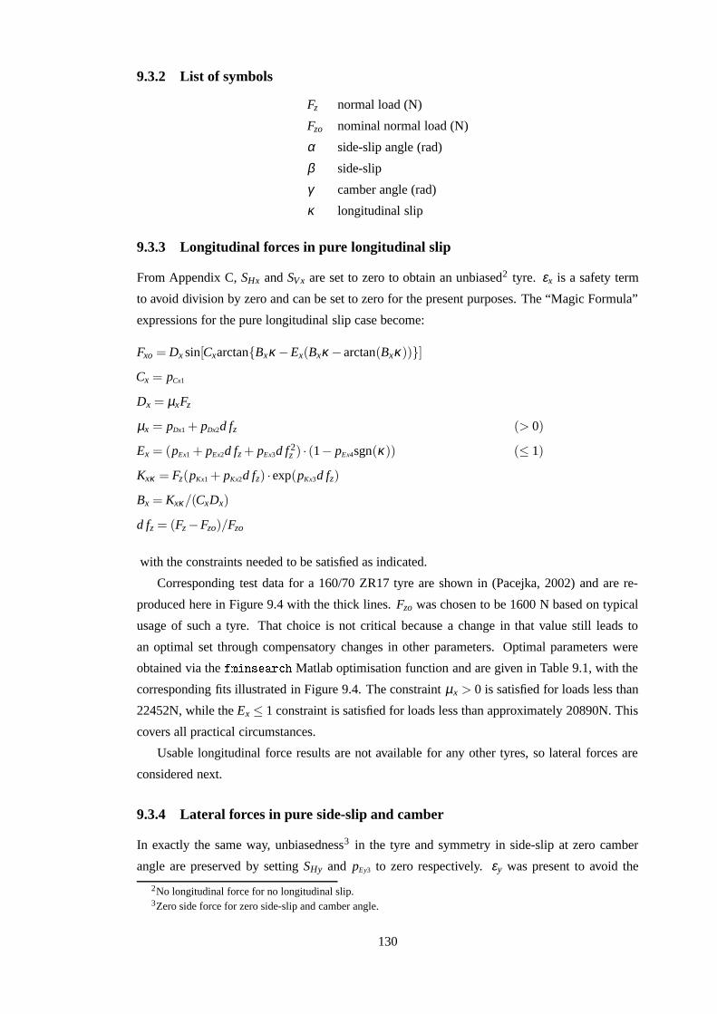
9.3.2 List of symbols
Fz normal load (N)
Fzo nominal normal load (N)
α side-slip angle (rad)
β side-slip
γ camber angle (rad)
κ longitudinal slip
9.3.3 Longitudinal forces in pure longitudinal slip
From Appendix C, SHx and SVx are set to zero to obtain an unbiased2 tyre. εx is a safety term
to avoid division by zero and can be set to zero for the present purposes. The “Magic Formula”
expressions for the pure longitudinal slip case become:
Fxo = Dx sin[Cxarctan{Bxκ −Ex(Bxκ − arctan(Bxκ))}]Cx = pCx1
Dx = µxFz
µx = pDx1 + pDx2d fz (> 0)
Ex = (pEx1 + pEx2d fz + pEx3d f 2z ) · (1− pEx4sgn(κ)) (≤ 1)
Kxκ = Fz(pKx1 + pKx2d fz) · exp(pKx3d fz)
Bx = Kxκ/(CxDx)
d fz = (Fz −Fzo)/Fzo
with the constraints needed to be satisfied as indicated.
Corresponding test data for a 160/70 ZR17 tyre are shown in (Pacejka, 2002) and are re-
produced here in Figure 9.4 with the thick lines. Fzo was chosen to be 1600 N based on typical
usage of such a tyre. That choice is not critical because a change in that value still leads to
an optimal set through compensatory changes in other parameters. Optimal parameters were
obtained via the� � �
� � �� � H � Matlab optimisation function and are given in Table 9.1, with the
corresponding fits illustrated in Figure 9.4. The constraint µx > 0 is satisfied for loads less than
22452N, while the Ex ≤ 1 constraint is satisfied for loads less than approximately 20890N. This
covers all practical circumstances.
Usable longitudinal force results are not available for any other tyres, so lateral forces are
considered next.
9.3.4 Lateral forces in pure side-slip and camber
In exactly the same way, unbiasedness3 in the tyre and symmetry in side-slip at zero camber
angle are preserved by setting SHy and pEy3 to zero respectively. εy was present to avoid the
2No longitudinal force for no longitudinal slip.3Zero side force for zero side-slip and camber angle.
130
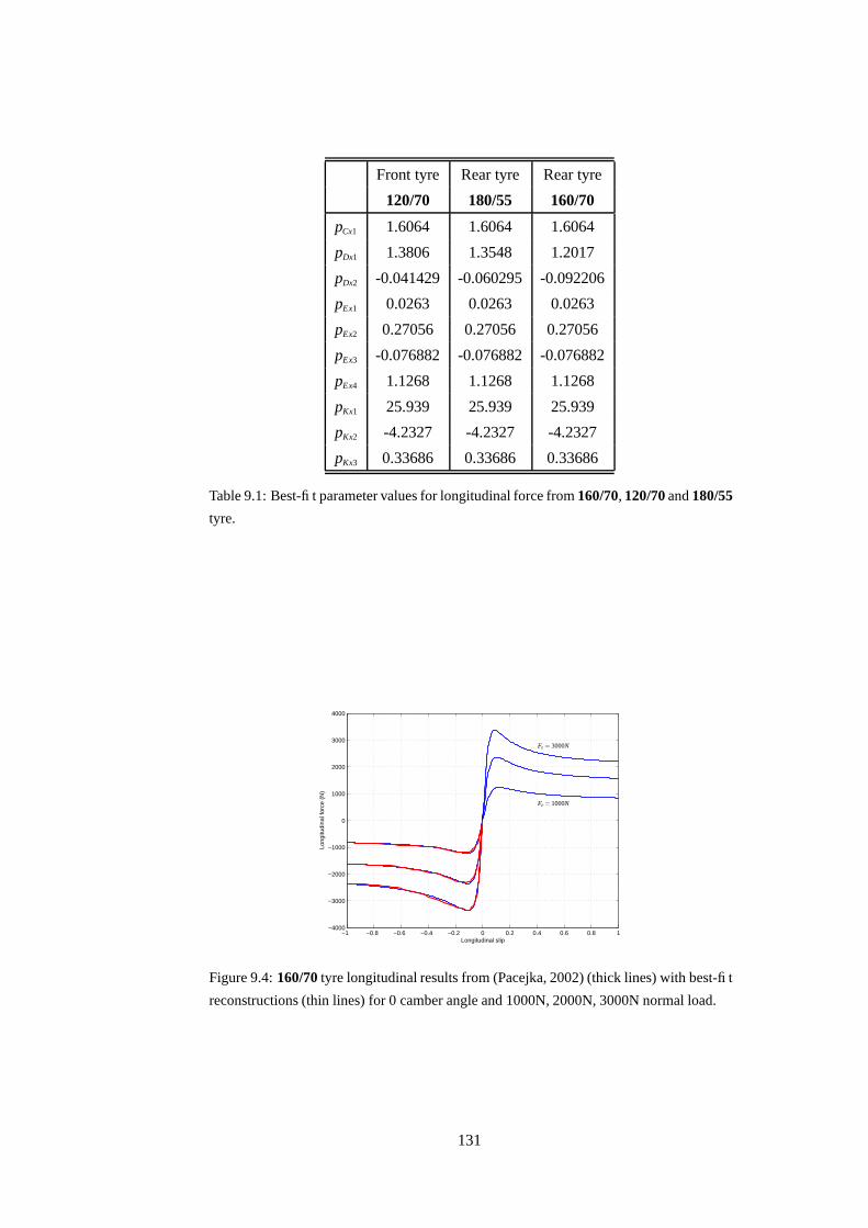
Front tyre Rear tyre Rear tyre
120/70 180/55 160/70
pCx1 1.6064 1.6064 1.6064
pDx1 1.3806 1.3548 1.2017
pDx2 -0.041429 -0.060295 -0.092206
pEx1 0.0263 0.0263 0.0263
pEx2 0.27056 0.27056 0.27056
pEx3 -0.076882 -0.076882 -0.076882
pEx4 1.1268 1.1268 1.1268
pKx1 25.939 25.939 25.939
pKx2 -4.2327 -4.2327 -4.2327
pKx3 0.33686 0.33686 0.33686
Table 9.1: Best-fit parameter values for longitudinal force from 160/70, 120/70 and 180/55
tyre.
−1 −0.8 −0.6 −0.4 −0.2 0 0.2 0.4 0.6 0.8 1−4000
−3000
−2000
−1000
0
1000
2000
3000
4000
Longitudinal slip
Long
itudi
nal f
orce
(N
)
Fz = 1000N
Fz = 3000N
Figure 9.4: 160/70 tyre longitudinal results from (Pacejka, 2002) (thick lines) with best-fit
reconstructions (thin lines) for 0 camber angle and 1000N, 2000N, 3000N normal load.
131
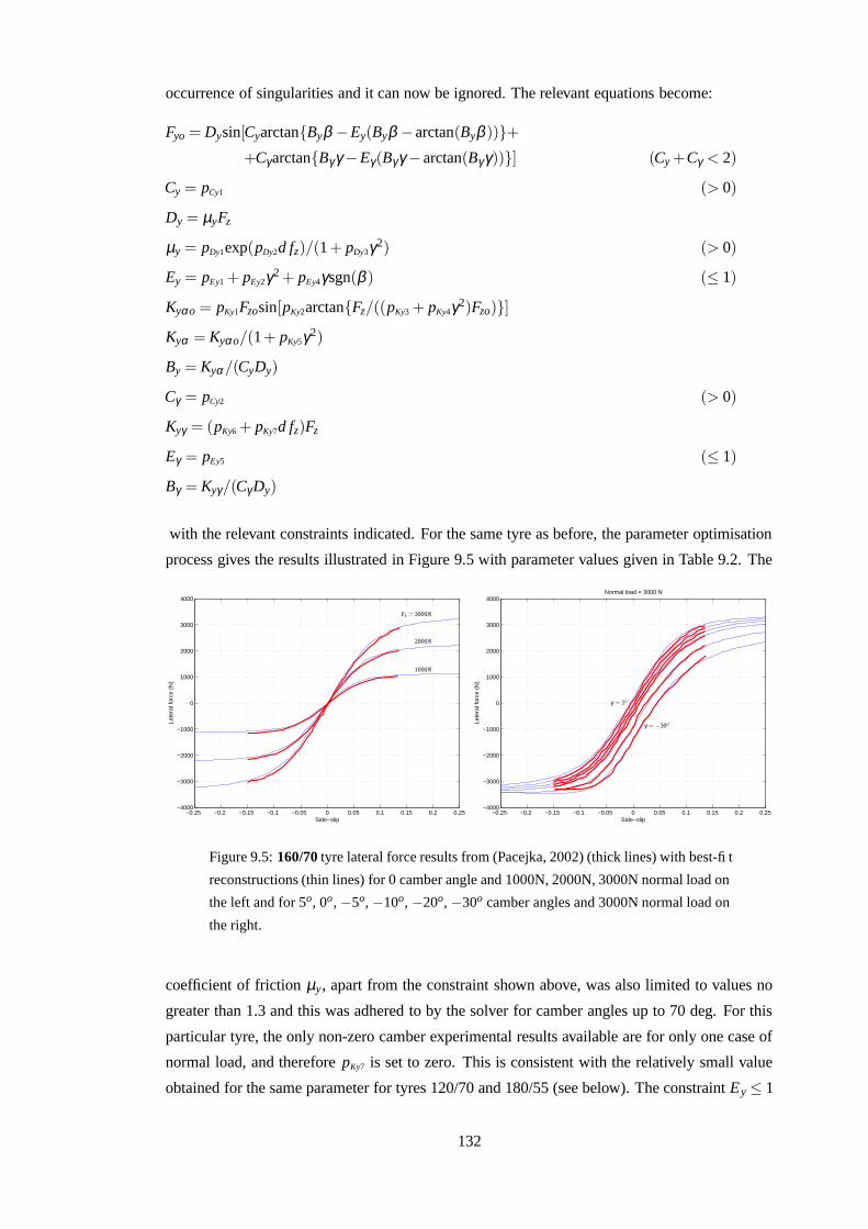
occurrence of singularities and it can now be ignored. The relevant equations become:
Fyo = Dysin[Cyarctan{Byβ −Ey(Byβ − arctan(Byβ ))}++Cγarctan{Bγ γ −Eγ(Bγγ − arctan(Bγ γ))}] (Cy +Cγ < 2)
Cy = pCy1 (> 0)
Dy = µyFz
µy = pDy1exp(pDy2d fz)/(1+ pDy3γ2) (> 0)
Ey = pEy1 + pEy2γ2 + pEy4γsgn(β ) (≤ 1)
Kyαo = pKy1Fzosin[pKy2arctan{Fz/((pKy3 + pKy4γ2)Fzo)}]Kyα = Kyαo/(1+ pKy5γ2)
By = Kyα/(CyDy)
Cγ = pCy2 (> 0)
Kyγ = (pKy6 + pKy7d fz)Fz
Eγ = pEy5 (≤ 1)
Bγ = Kyγ/(Cγ Dy)
with the relevant constraints indicated. For the same tyre as before, the parameter optimisation
process gives the results illustrated in Figure 9.5 with parameter values given in Table 9.2. The
−0.25 −0.2 −0.15 −0.1 −0.05 0 0.05 0.1 0.15 0.2 0.25−4000
−3000
−2000
−1000
0
1000
2000
3000
4000
Side−slip
Late
ral f
orce
(N
)
1000N
2000N
Fz = 3000N
−0.25 −0.2 −0.15 −0.1 −0.05 0 0.05 0.1 0.15 0.2 0.25−4000
−3000
−2000
−1000
0
1000
2000
3000
4000
Side−slip
Late
ral f
orce
(N
)
Normal load = 3000 N
γ = −30o
γ = 5o
Figure 9.5: 160/70 tyre lateral force results from (Pacejka, 2002) (thick lines) with best-fit
reconstructions (thin lines) for 0 camber angle and 1000N, 2000N, 3000N normal load on
the left and for 5o, 0o, −5o, −10o, −20o, −30o camber angles and 3000N normal load on
the right.
coefficient of friction µy, apart from the constraint shown above, was also limited to values no
greater than 1.3 and this was adhered to by the solver for camber angles up to 70 deg. For this
particular tyre, the only non-zero camber experimental results available are for only one case of
normal load, and therefore pKy7 is set to zero. This is consistent with the relatively small value
obtained for the same parameter for tyres 120/70 and 180/55 (see below). The constraint Ey ≤ 1
132
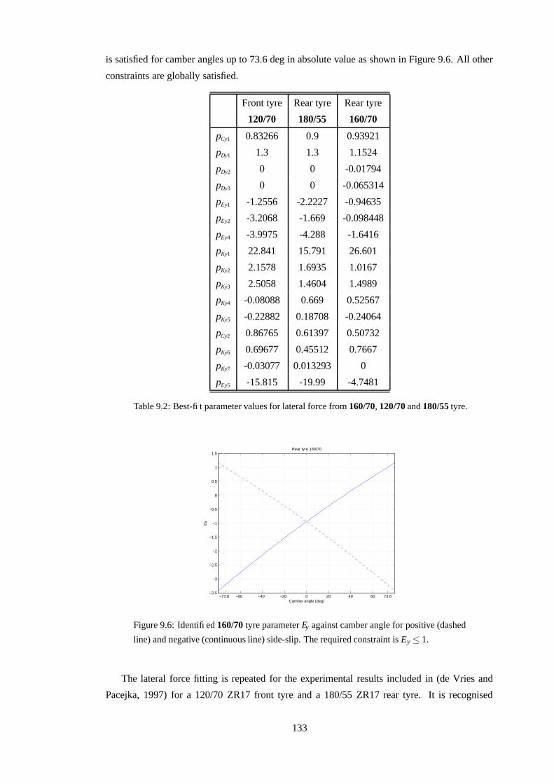
is satisfied for camber angles up to 73.6 deg in absolute value as shown in Figure 9.6. All other
constraints are globally satisfied.
Front tyre Rear tyre Rear tyre
120/70 180/55 160/70
pCy1 0.83266 0.9 0.93921
pDy1 1.3 1.3 1.1524
pDy2 0 0 -0.01794
pDy3 0 0 -0.065314
pEy1 -1.2556 -2.2227 -0.94635
pEy2 -3.2068 -1.669 -0.098448
pEy4 -3.9975 -4.288 -1.6416
pKy1 22.841 15.791 26.601
pKy2 2.1578 1.6935 1.0167
pKy3 2.5058 1.4604 1.4989
pKy4 -0.08088 0.669 0.52567
pKy5 -0.22882 0.18708 -0.24064
pCy2 0.86765 0.61397 0.50732
pKy6 0.69677 0.45512 0.7667
pKy7 -0.03077 0.013293 0
pEy5 -15.815 -19.99 -4.7481
Table 9.2: Best-fit parameter values for lateral force from 160/70, 120/70 and 180/55 tyre.
−73.6 −60 −40 −20 0 20 40 60 73.6−3.5
−3
−2.5
−2
−1.5
−1
−0.5
0
0.5
1
1.5
Camber angle (deg)
Ey
Rear tyre 160/70
Figure 9.6: Identified 160/70 tyre parameter Ey against camber angle for positive (dashed
line) and negative (continuous line) side-slip. The required constraint is Ey ≤ 1.
The lateral force fitting is repeated for the experimental results included in (de Vries and
Pacejka, 1997) for a 120/70 ZR17 front tyre and a 180/55 ZR17 rear tyre. It is recognised
133
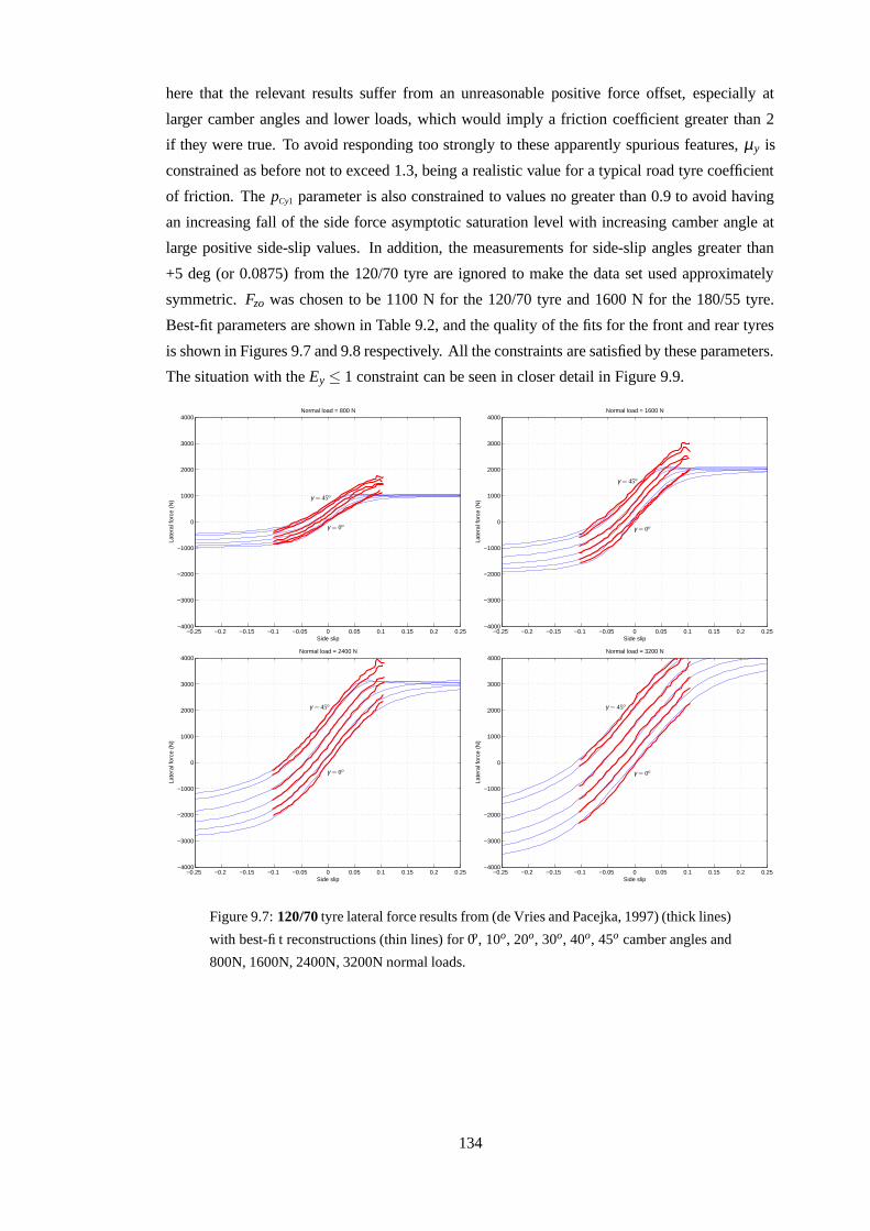
here that the relevant results suffer from an unreasonable positive force offset, especially at
larger camber angles and lower loads, which would imply a friction coefficient greater than 2
if they were true. To avoid responding too strongly to these apparently spurious features, µy is
constrained as before not to exceed 1.3, being a realistic value for a typical road tyre coefficient
of friction. The pCy1 parameter is also constrained to values no greater than 0.9 to avoid having
an increasing fall of the side force asymptotic saturation level with increasing camber angle at
large positive side-slip values. In addition, the measurements for side-slip angles greater than
+5 deg (or 0.0875) from the 120/70 tyre are ignored to make the data set used approximately
symmetric. Fzo was chosen to be 1100 N for the 120/70 tyre and 1600 N for the 180/55 tyre.
Best-fit parameters are shown in Table 9.2, and the quality of the fits for the front and rear tyres
is shown in Figures 9.7 and 9.8 respectively. All the constraints are satisfied by these parameters.
The situation with the Ey ≤ 1 constraint can be seen in closer detail in Figure 9.9.
−0.25 −0.2 −0.15 −0.1 −0.05 0 0.05 0.1 0.15 0.2 0.25−4000
−3000
−2000
−1000
0
1000
2000
3000
4000
Side slip
Late
ral f
orce
(N
)
Normal load = 800 N
γ = 0o
γ = 45o
−0.25 −0.2 −0.15 −0.1 −0.05 0 0.05 0.1 0.15 0.2 0.25−4000
−3000
−2000
−1000
0
1000
2000
3000
4000
Side slip
Late
ral f
orce
(N
)
Normal load = 1600 N
γ = 0o
γ = 45o
−0.25 −0.2 −0.15 −0.1 −0.05 0 0.05 0.1 0.15 0.2 0.25−4000
−3000
−2000
−1000
0
1000
2000
3000
4000
Side slip
Late
ral f
orce
(N
)
Normal load = 2400 N
γ = 0o
γ = 45o
−0.25 −0.2 −0.15 −0.1 −0.05 0 0.05 0.1 0.15 0.2 0.25−4000
−3000
−2000
−1000
0
1000
2000
3000
4000
Side slip
Late
ral f
orce
(N
)
Normal load = 3200 N
γ = 0o
γ = 45o
Figure 9.7: 120/70 tyre lateral force results from (de Vries and Pacejka, 1997) (thick lines)
with best-fit reconstructions (thin lines) for 0o, 10o, 20o, 30o, 40o, 45o camber angles and
800N, 1600N, 2400N, 3200N normal loads.
134
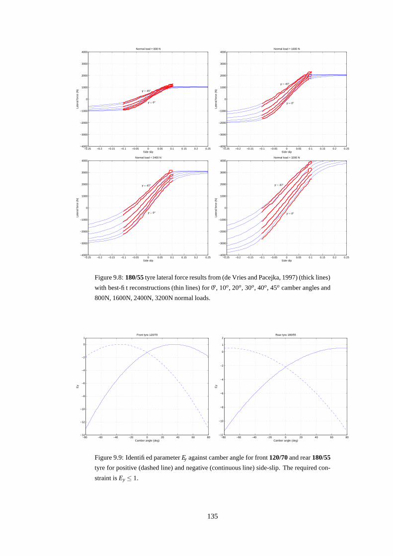
−0.25 −0.2 −0.15 −0.1 −0.05 0 0.05 0.1 0.15 0.2 0.25−4000
−3000
−2000
−1000
0
1000
2000
3000
4000
Side slip
Late
ral f
orce
(N
)
Normal load = 800 N
γ = 0o
γ = 45o
−0.25 −0.2 −0.15 −0.1 −0.05 0 0.05 0.1 0.15 0.2 0.25−4000
−3000
−2000
−1000
0
1000
2000
3000
4000
Side slip
Late
ral f
orce
(N
)
Normal load = 1600 N
γ = 0o
γ = 45o
−0.25 −0.2 −0.15 −0.1 −0.05 0 0.05 0.1 0.15 0.2 0.25−4000
−3000
−2000
−1000
0
1000
2000
3000
4000
Side slip
Late
ral f
orce
(N
)
Normal load = 2400 N
γ = 0o
γ = 45o
−0.25 −0.2 −0.15 −0.1 −0.05 0 0.05 0.1 0.15 0.2 0.25−4000
−3000
−2000
−1000
0
1000
2000
3000
4000
Side slip
Late
ral f
orce
(N
)
Normal load = 3200 N
γ = 0o
γ = 45o
Figure 9.8: 180/55 tyre lateral force results from (de Vries and Pacejka, 1997) (thick lines)
with best-fit reconstructions (thin lines) for 0o, 10o, 20o, 30o, 40o, 45o camber angles and
800N, 1600N, 2400N, 3200N normal loads.
−80 −60 −40 −20 0 20 40 60 80−14
−12
−10
−8
−6
−4
−2
0
1
Camber angle (deg)
Ey
Front tyre 120/70
−80 −60 −40 −20 0 20 40 60 80−12
−10
−8
−6
−4
−2
0
1
2
Camber angle (deg)
Ey
Rear tyre 180/55
Figure 9.9: Identified parameter Ey against camber angle for front 120/70 and rear 180/55
tyre for positive (dashed line) and negative (continuous line) side-slip. The required con-
straint is Ey ≤ 1.
135
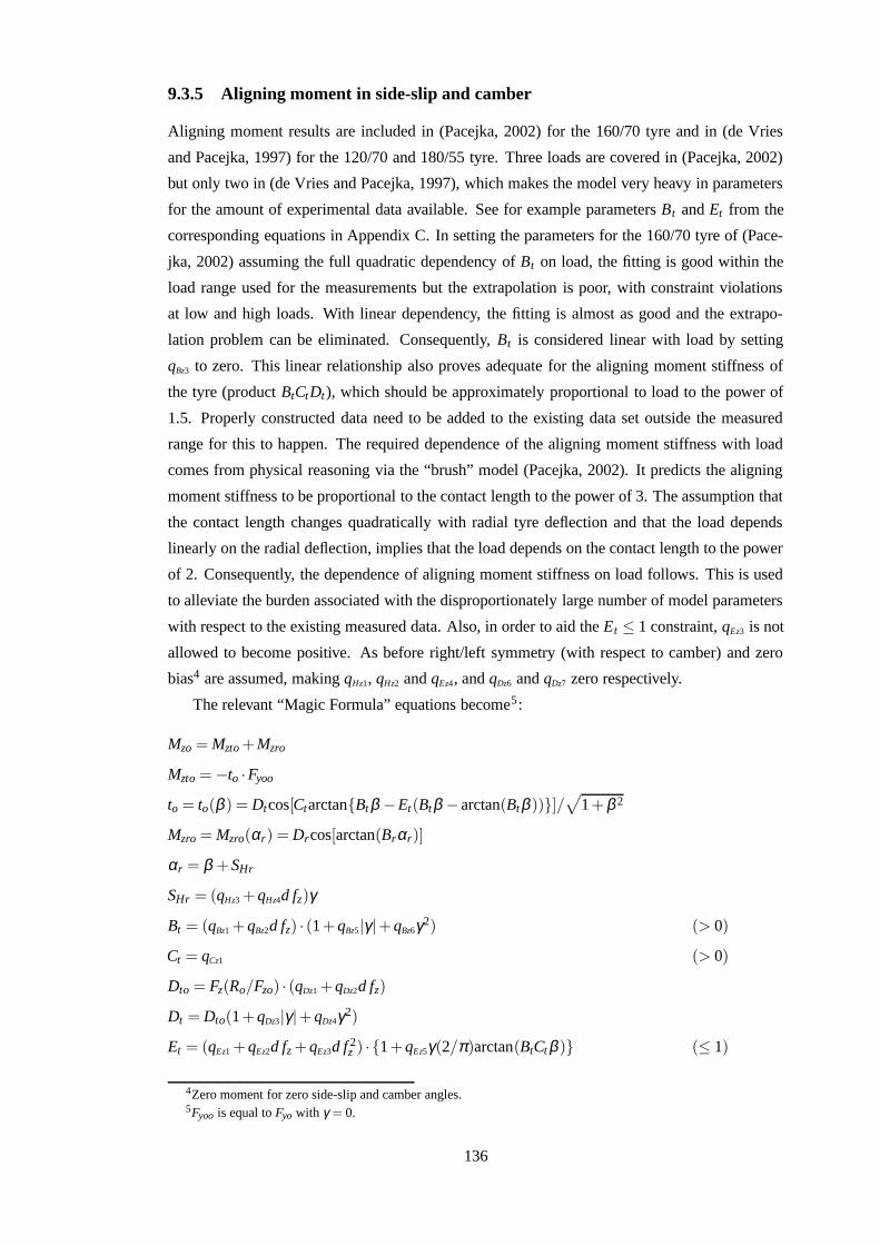
9.3.5 Aligning moment in side-slip and camber
Aligning moment results are included in (Pacejka, 2002) for the 160/70 tyre and in (de Vries
and Pacejka, 1997) for the 120/70 and 180/55 tyre. Three loads are covered in (Pacejka, 2002)
but only two in (de Vries and Pacejka, 1997), which makes the model very heavy in parameters
for the amount of experimental data available. See for example parameters Bt and Et from the
corresponding equations in Appendix C. In setting the parameters for the 160/70 tyre of (Pace-
jka, 2002) assuming the full quadratic dependency of Bt on load, the fitting is good within the
load range used for the measurements but the extrapolation is poor, with constraint violations
at low and high loads. With linear dependency, the fitting is almost as good and the extrapo-
lation problem can be eliminated. Consequently, Bt is considered linear with load by setting
qBz3 to zero. This linear relationship also proves adequate for the aligning moment stiffness of
the tyre (product BtCtDt ), which should be approximately proportional to load to the power of
1.5. Properly constructed data need to be added to the existing data set outside the measured
range for this to happen. The required dependence of the aligning moment stiffness with load
comes from physical reasoning via the “brush” model (Pacejka, 2002). It predicts the aligning
moment stiffness to be proportional to the contact length to the power of 3. The assumption that
the contact length changes quadratically with radial tyre deflection and that the load depends
linearly on the radial deflection, implies that the load depends on the contact length to the power
of 2. Consequently, the dependence of aligning moment stiffness on load follows. This is used
to alleviate the burden associated with the disproportionately large number of model parameters
with respect to the existing measured data. Also, in order to aid the Et ≤ 1 constraint, qEz3 is not
allowed to become positive. As before right/left symmetry (with respect to camber) and zero
bias4 are assumed, making qHz1, qHz2 and qEz4, and qDz6 and qDz7 zero respectively.
The relevant “Magic Formula” equations become5:
Mzo = Mzto +Mzro
Mzto = −to ·Fyoo
to = to(β ) = Dtcos[Ctarctan{Bt β −Et(Btβ − arctan(Btβ ))}]/√
1+β 2
Mzro = Mzro(αr) = Drcos[arctan(Brαr)]
αr = β +SHr
SHr = (qHz3 +qHz4d fz)γ
Bt = (qBz1 +qBz2d fz) · (1+qBz5|γ |+qBz6γ2) (> 0)
Ct = qCz1 (> 0)
Dto = Fz(Ro/Fzo) · (qDz1 +qDz2d fz)
Dt = Dto(1+qDz3|γ |+qDz4γ2)
Et = (qEz1 +qEz2d fz +qEz3d f 2z ) · {1+qEz5γ(2/π)arctan(BtCt β )} (≤ 1)
4Zero moment for zero side-slip and camber angles.5Fyoo is equal to Fyo with γ = 0.
136
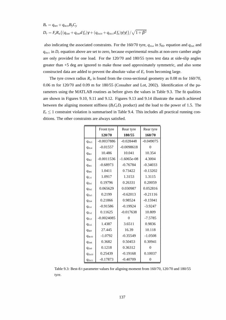
Br = qBz9 +qBz10ByCy
Dr = FzRo{(qDz8 +qDz9d fz)γ +(qDz10 +qDz11d fz)γ |γ |}/√
1+β 2
also indicating the associated constraints. For the 160/70 tyre, qHz4 in SHr equation and qDz9 and
qDz11 in Dr equation above are set to zero, because experimental results at non-zero camber angle
are only provided for one load. For the 120/70 and 180/55 tyres test data at side-slip angles
greater than +5 deg are ignored to make those used approximately symmetric, and also some
constructed data are added to prevent the absolute value of Et from becoming large.
The tyre crown radius Ro is found from the cross-sectional geometry as 0.08 m for 160/70,
0.06 m for 120/70 and 0.09 m for 180/55 (Cossalter and Lot, 2002). Identification of the pa-
rameters using the MATLAB routines as before gives the values in Table 9.3. The fit qualities
are shown in Figures 9.10, 9.11 and 9.12. Figures 9.13 and 9.14 illustrate the match achieved
between the aligning moment stiffness (BtCtDt product) and the load to the power of 1.5. The
Et ≤ 1 constraint violation is summarised in Table 9.4. This includes all practical running con-
ditions. The other constraints are always satisfied.
Front tyre Rear tyre Rear tyre
120/70 180/55 160/70
qHz3 -0.0037886 -0.028448 -0.049075
qHz4 -0.01557 -0.0098618 0
qBz1 10.486 10.041 10.354
qBz2 -0.0011536 -1.6065e-08 4.3004
qBz5 -0.68973 -0.76784 -0.34033
qBz6 1.0411 0.73422 -0.13202
qCz1 1.0917 1.3153 1.3115
qDz1 0.19796 0.26331 0.20059
qDz2 0.065629 0.030987 0.052816
qDz3 0.2199 -0.62013 -0.21116
qDz4 0.21866 0.98524 -0.15941
qEz1 -0.91586 -0.19924 -3.9247
qEz2 0.11625 -0.017638 10.809
qEz3 -0.0024085 0 -7.5785
qEz5 1.4387 3.6511 0.9836
qBz9 27.445 16.39 10.118
qBz10 -1.0792 -0.35549 -1.0508
qDz8 0.3682 0.50453 0.30941
qDz9 0.1218 0.36312 0
qDz10 0.25439 -0.19168 0.10037
qDz11 -0.17873 -0.40709 0
Table 9.3: Best-fit parameter values for aligning moment from 160/70, 120/70 and 180/55
tyre.
137
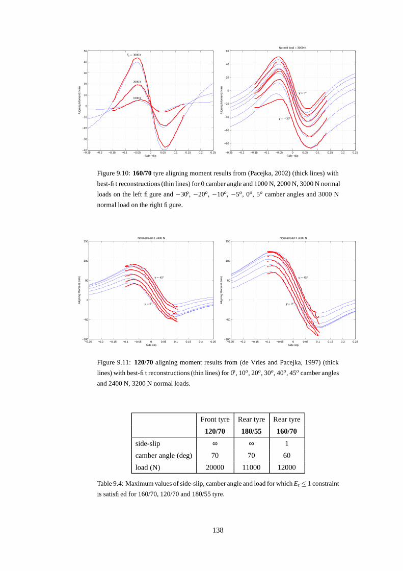
−0.25 −0.2 −0.15 −0.1 −0.05 0 0.05 0.1 0.15 0.2 0.25−40
−30
−20
−10
0
10
20
30
40
50
Side−slip
Alig
ning
Mom
ent (
Nm
)
1000N
2000N
Fz = 3000N
−0.25 −0.2 −0.15 −0.1 −0.05 0 0.05 0.1 0.15 0.2 0.25
−80
−60
−40
−20
0
20
40
60
Side−slip
Alig
ning
Mom
ent (
Nm
)
Normal load = 3000 N
γ = −30o
γ = 5o
Figure 9.10: 160/70 tyre aligning moment results from (Pacejka, 2002) (thick lines) with
best-fit reconstructions (thin lines) for 0 camber angle and 1000 N, 2000 N, 3000 N normal
loads on the left figure and −30o, −20o, −10o, −5o, 0o, 5o camber angles and 3000 N
normal load on the right figure.
−0.25 −0.2 −0.15 −0.1 −0.05 0 0.05 0.1 0.15 0.2 0.25−100
−50
0
50
100
150
Side slip
Alig
ning
Mom
ent (
Nm
)
Normal load = 2400 N
γ = 0o
γ = 45o
−0.25 −0.2 −0.15 −0.1 −0.05 0 0.05 0.1 0.15 0.2 0.25−100
−50
0
50
100
150
Side slip
Alig
ning
Mom
ent (
Nm
)
Normal load = 3200 N
γ = 0o
γ = 45o
Figure 9.11: 120/70 aligning moment results from (de Vries and Pacejka, 1997) (thick
lines) with best-fit reconstructions (thin lines) for 0o, 10o, 20o, 30o, 40o, 45o camber angles
and 2400 N, 3200 N normal loads.
Front tyre Rear tyre Rear tyre
120/70 180/55 160/70
side-slip ∞ ∞ 1
camber angle (deg) 70 70 60
load (N) 20000 11000 12000
Table 9.4: Maximum values of side-slip, camber angle and load for which Et ≤ 1 constraint
is satisfied for 160/70, 120/70 and 180/55 tyre.
138
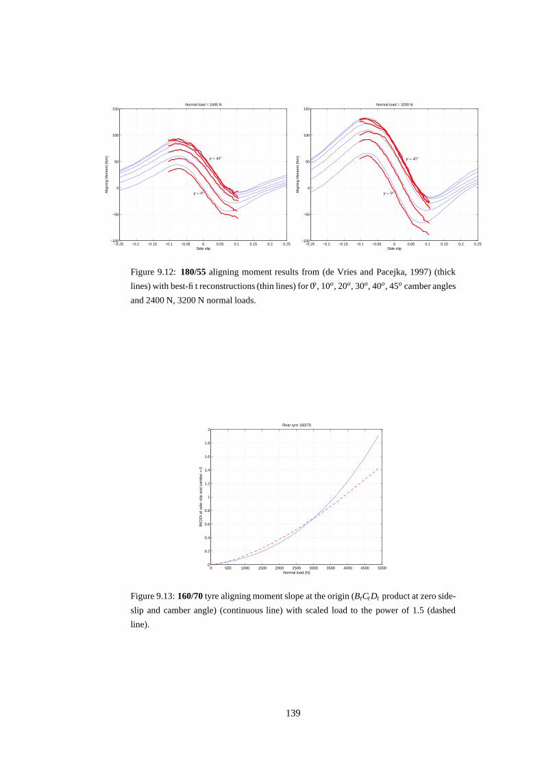
−0.25 −0.2 −0.15 −0.1 −0.05 0 0.05 0.1 0.15 0.2 0.25−100
−50
0
50
100
150
Side slip
Alig
ning
Mom
ent (
Nm
)Normal load = 2400 N
γ = 0o
γ = 45o
−0.25 −0.2 −0.15 −0.1 −0.05 0 0.05 0.1 0.15 0.2 0.25−100
−50
0
50
100
150
Side slip
Alig
ning
Mom
ent (
Nm
)
Normal load = 3200 N
γ = 0o
γ = 45o
Figure 9.12: 180/55 aligning moment results from (de Vries and Pacejka, 1997) (thick
lines) with best-fit reconstructions (thin lines) for 0o, 10o, 20o, 30o, 40o, 45o camber angles
and 2400 N, 3200 N normal loads.
0 500 1000 1500 2000 2500 3000 3500 4000 4500 50000
0.2
0.4
0.6
0.8
1
1.2
1.4
1.6
1.8
2
Normal load (N)
BtC
tDt a
t sid
e−sl
ip a
nd c
ambe
r =
0
Rear tyre 160/70
Figure 9.13: 160/70 tyre aligning moment slope at the origin (BtCt Dt product at zero side-
slip and camber angle) (continuous line) with scaled load to the power of 1.5 (dashed
line).
139
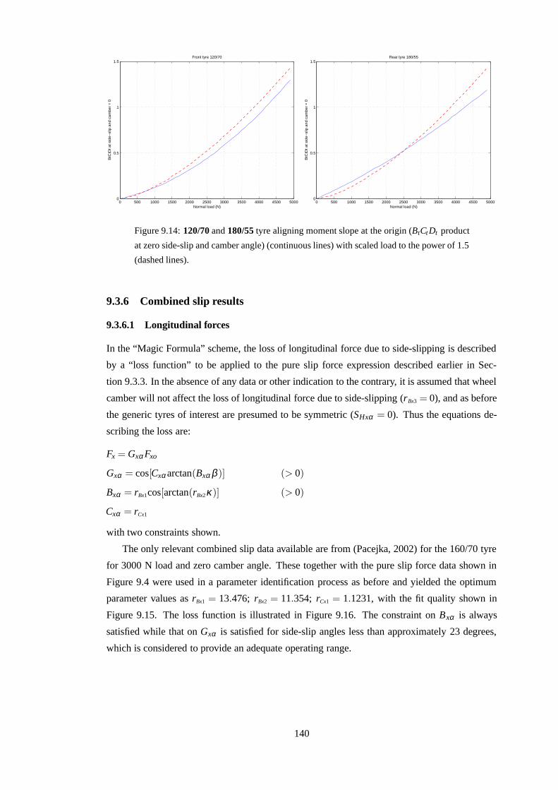
0 500 1000 1500 2000 2500 3000 3500 4000 4500 50000
0.5
1
1.5
Normal load (N)
BtC
tDt a
t sid
e−sl
ip a
nd c
ambe
r =
0
Front tyre 120/70
0 500 1000 1500 2000 2500 3000 3500 4000 4500 50000
0.5
1
1.5
Normal load (N)
BtC
tDt a
t sid
e−sl
ip a
nd c
ambe
r =
0
Rear tyre 180/55
Figure 9.14: 120/70 and 180/55 tyre aligning moment slope at the origin (BtCt Dt product
at zero side-slip and camber angle) (continuous lines) with scaled load to the power of 1.5
(dashed lines).
9.3.6 Combined slip results
9.3.6.1 Longitudinal forces
In the “Magic Formula” scheme, the loss of longitudinal force due to side-slipping is described
by a “loss function” to be applied to the pure slip force expression described earlier in Sec-
tion 9.3.3. In the absence of any data or other indication to the contrary, it is assumed that wheel
camber will not affect the loss of longitudinal force due to side-slipping (rBx3 = 0), and as before
the generic tyres of interest are presumed to be symmetric (SHxα = 0). Thus the equations de-
scribing the loss are:
Fx = Gxα Fxo
Gxα = cos[Cxα arctan(Bxα β )] (> 0)
Bxα = rBx1cos[arctan(rBx2κ)] (> 0)
Cxα = rCx1
with two constraints shown.
The only relevant combined slip data available are from (Pacejka, 2002) for the 160/70 tyre
for 3000 N load and zero camber angle. These together with the pure slip force data shown in
Figure 9.4 were used in a parameter identification process as before and yielded the optimum
parameter values as rBx1 = 13.476; rBx2 = 11.354; rCx1 = 1.1231, with the fit quality shown in
Figure 9.15. The loss function is illustrated in Figure 9.16. The constraint on Bxα is always
satisfied while that on Gxα is satisfied for side-slip angles less than approximately 23 degrees,
which is considered to provide an adequate operating range.
140
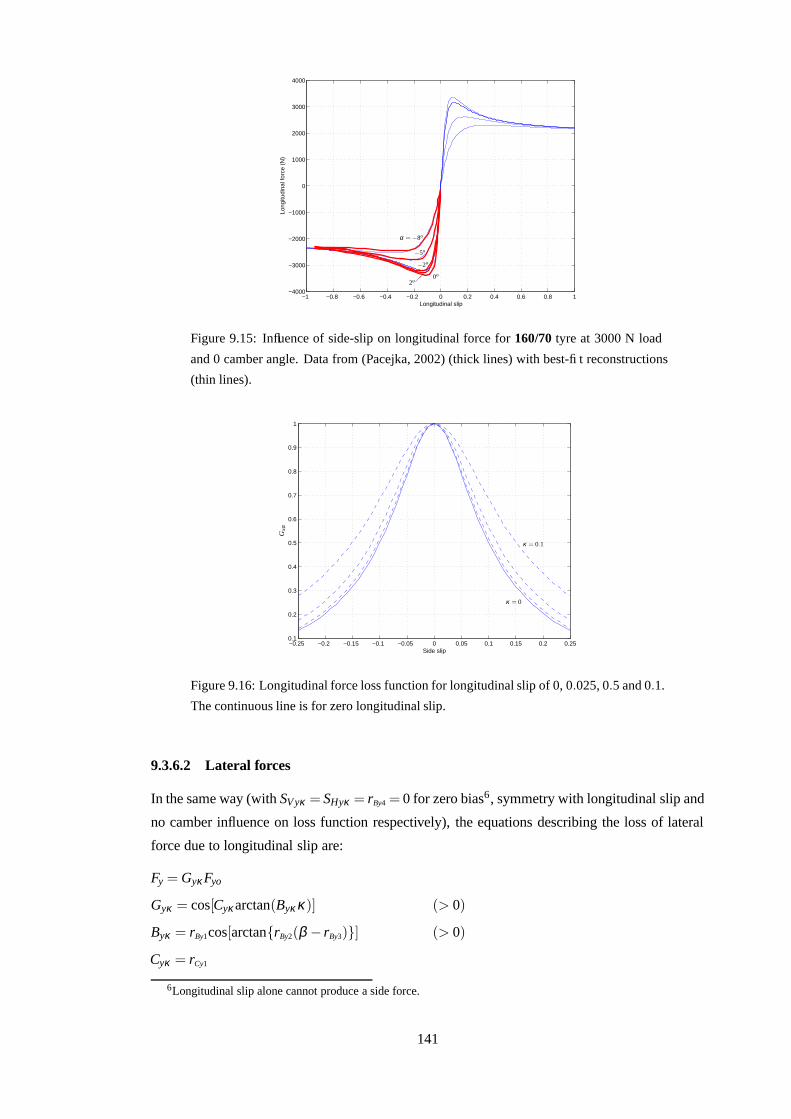
−1 −0.8 −0.6 −0.4 −0.2 0 0.2 0.4 0.6 0.8 1−4000
−3000
−2000
−1000
0
1000
2000
3000
4000
Longitudinal slip
Long
itudi
nal f
orce
(N
)��
2o0o
−2o
−5o
α = −8o
Figure 9.15: Influence of side-slip on longitudinal force for 160/70 tyre at 3000 N load
and 0 camber angle. Data from (Pacejka, 2002) (thick lines) with best-fit reconstructions
(thin lines).
−0.25 −0.2 −0.15 −0.1 −0.05 0 0.05 0.1 0.15 0.2 0.250.1
0.2
0.3
0.4
0.5
0.6
0.7
0.8
0.9
1
Side slip
PSfrag replacements
κ = 0
0.1
Gxα
κ = 0
κ = 0.1
Figure 9.16: Longitudinal force loss function for longitudinal slip of 0, 0.025, 0.5 and 0.1.
The continuous line is for zero longitudinal slip.
9.3.6.2 Lateral forces
In the same way (with SVyκ = SHyκ = rBy4 = 0 for zero bias6, symmetry with longitudinal slip and
no camber influence on loss function respectively), the equations describing the loss of lateral
force due to longitudinal slip are:
Fy = Gyκ Fyo
Gyκ = cos[Cyκ arctan(Byκ κ)] (> 0)
Byκ = rBy1cos[arctan{rBy2(β − rBy3)}] (> 0)
Cyκ = rCy1
6Longitudinal slip alone cannot produce a side force.
141
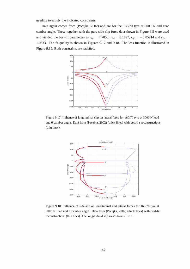
needing to satisfy the indicated constraints.
Data again comes from (Pacejka, 2002) and are for the 160/70 tyre at 3000 N and zero
camber angle. These together with the pure side-slip force data shown in Figure 9.5 were used
and yielded the best-fit parameters as rBy1 = 7.7856, rBy2 = 8.1697, rBy3 = −0.05914 and rCy1 =
1.0533. The fit quality is shown in Figures 9.17 and 9.18. The loss function is illustrated in
Figure 9.19. Both constraints are satisfied.
−1 −0.8 −0.6 −0.4 −0.2 0 0.2 0.4 0.6 0.8 1−3000
−2500
−2000
−1500
−1000
−500
0
500
1000
1500
Longitudinal slip
Late
ral f
orce
(N
)
α = 2o
0o
−2o
−5o
−8o
Figure 9.17: Influence of longitudinal slip on lateral force for 160/70 tyre at 3000 N load
and 0 camber angle. Data from (Pacejka, 2002) (thick lines) with best-fit reconstructions
(thin lines).
−3000 −2000 −1000 0 1000 2000 3000−3000
−2500
−2000
−1500
−1000
−500
0
500
1000
1500
Longitudinal Force (N)
Late
ral F
orce
(N
)
Normal load = 3000 N
α = 2o
0o
−2o
−5o
−8o
Figure 9.18: Influence of side-slip on longitudinal and lateral forces for 160/70 tyre at
3000 N load and 0 camber angle. Data from (Pacejka, 2002) (thick lines) with best-fit
reconstructions (thin lines). The longitudinal slip varies from -1 to 1.
142
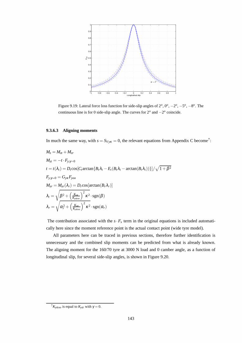
−1 −0.8 −0.6 −0.4 −0.2 0 0.2 0.4 0.6 0.8 10
0.1
0.2
0.3
0.4
0.5
0.6
0.7
0.8
0.9
1
Longitudinal slip
PSfrag replacements
Gyk
α = 2o
Figure 9.19: Lateral force loss function for side-slip angles of 2o, 0o, −2o, −5o, −8o. The
continuous line is for 0 side-slip angle. The curves for 2o and −2o coincide.
9.3.6.3 Aligning moments
In much the same way, with s = SVyκ = 0, the relevant equations from Appendix C become7:
Mz = Mzt +Mzr
Mzt = −t ·Fy,γ=0
t = t(λt) = Dtcos[Ctarctan{Bt λt −Et(Btλt − arctan(Bt λt))}]/√
1+β 2
Fy,γ=0 = Gyκ Fyoo
Mzr = Mzr(λr) = Drcos[arctan(Brλr)]
λt =
√
β 2 +(
KxκKyαoo
)2κ2 · sgn(β )
λr =
√
α2r +(
KxκKyαoo
)2κ2 · sgn(αr)
The contribution associated with the s ·Fx term in the original equations is included automati-
cally here since the moment reference point is the actual contact point (wide tyre model).
All parameters here can be traced in previous sections, therefore further identification is
unnecessary and the combined slip moments can be predicted from what is already known.
The aligning moment for the 160/70 tyre at 3000 N load and 0 camber angle, as a function of
longitudinal slip, for several side-slip angles, is shown in Figure 9.20.
7Kyαoo is equal to Kyα with γ = 0.
143
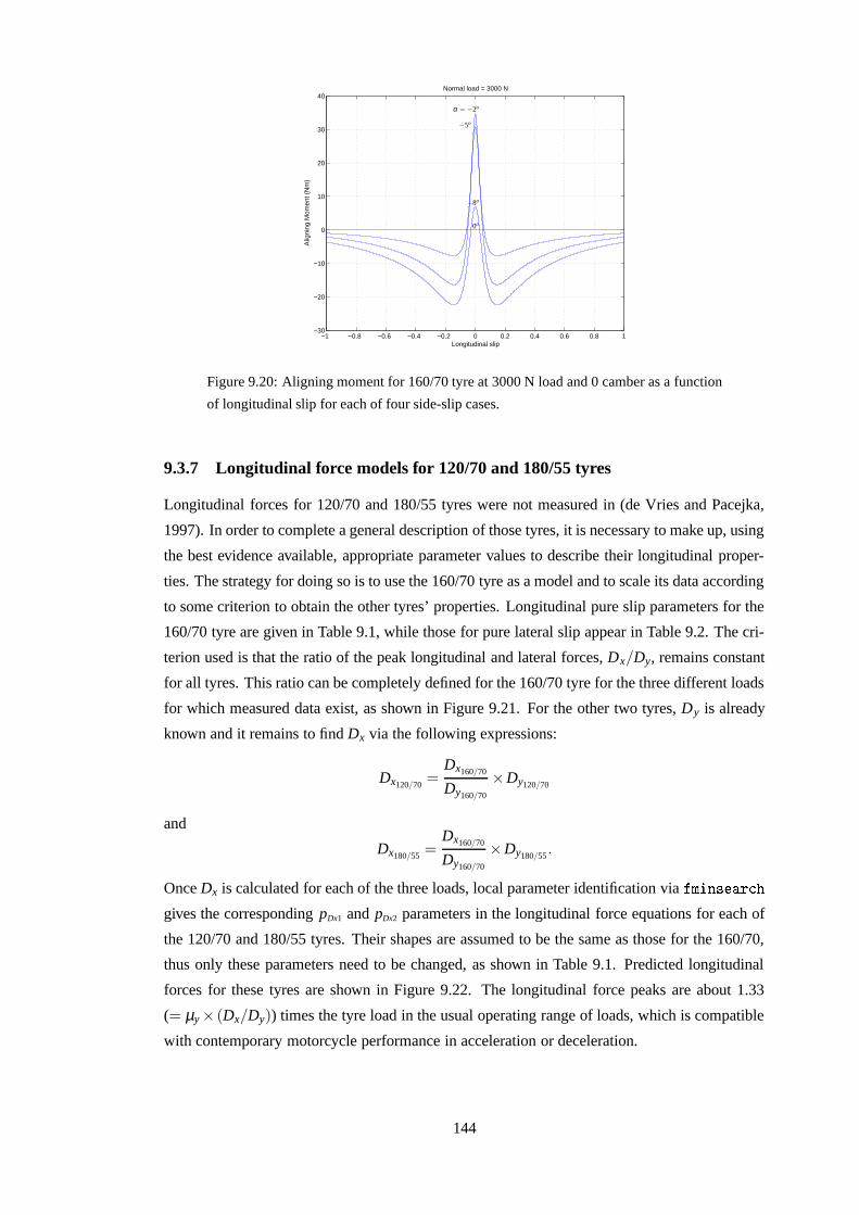
−1 −0.8 −0.6 −0.4 −0.2 0 0.2 0.4 0.6 0.8 1−30
−20
−10
0
10
20
30
40
Longitudinal slip
Alig
ning
Mom
ent (
Nm
)
Normal load = 3000 N
α = −2o
−8o
−5o
0o
Figure 9.20: Aligning moment for 160/70 tyre at 3000 N load and 0 camber as a function
of longitudinal slip for each of four side-slip cases.
9.3.7 Longitudinal force models for 120/70 and 180/55 tyres
Longitudinal forces for 120/70 and 180/55 tyres were not measured in (de Vries and Pacejka,
1997). In order to complete a general description of those tyres, it is necessary to make up, using
the best evidence available, appropriate parameter values to describe their longitudinal proper-
ties. The strategy for doing so is to use the 160/70 tyre as a model and to scale its data according
to some criterion to obtain the other tyres’ properties. Longitudinal pure slip parameters for the
160/70 tyre are given in Table 9.1, while those for pure lateral slip appear in Table 9.2. The cri-
terion used is that the ratio of the peak longitudinal and lateral forces, Dx/Dy, remains constant
for all tyres. This ratio can be completely defined for the 160/70 tyre for the three different loads
for which measured data exist, as shown in Figure 9.21. For the other two tyres, Dy is already
known and it remains to find Dx via the following expressions:
Dx120/70=
Dx160/70
Dy160/70
×Dy120/70
and
Dx180/55=
Dx160/70
Dy160/70
×Dy180/55.
Once Dx is calculated for each of the three loads, local parameter identification via� � �
� � �� � H �gives the corresponding pDx1 and pDx2 parameters in the longitudinal force equations for each of
the 120/70 and 180/55 tyres. Their shapes are assumed to be the same as those for the 160/70,
thus only these parameters need to be changed, as shown in Table 9.1. Predicted longitudinal
forces for these tyres are shown in Figure 9.22. The longitudinal force peaks are about 1.33
(= µy × (Dx/Dy)) times the tyre load in the usual operating range of loads, which is compatible
with contemporary motorcycle performance in acceleration or deceleration.
144
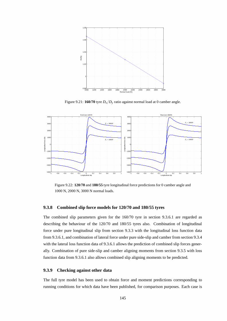
1000 1200 1400 1600 1800 2000 2200 2400 2600 2800 30000.98
1
1.02
1.04
1.06
1.08
Dx/
Dy
PSfrag replacements
Normal load (N)
Figure 9.21: 160/70 tyre Dx/Dy ratio against normal load at 0 camber angle.
−1 −0.8 −0.6 −0.4 −0.2 0 0.2 0.4 0.6 0.8 1−4000
−3000
−2000
−1000
0
1000
2000
3000
4000
Longitudinal slip
Long
itudi
nal f
orce
(N
)
Front tyre 120/70
Fz = 1000N
Fz = 3000N
−1 −0.8 −0.6 −0.4 −0.2 0 0.2 0.4 0.6 0.8 1−4000
−3000
−2000
−1000
0
1000
2000
3000
4000
Longitudinal slip
Long
itudi
nal f
orce
(N
)
Rear tyre 180/55
Fz = 1000N
Fz = 3000N
Figure 9.22: 120/70 and 180/55 tyre longitudinal force predictions for 0 camber angle and
1000 N, 2000 N, 3000 N normal loads.
9.3.8 Combined slip force models for 120/70 and 180/55 tyres
The combined slip parameters given for the 160/70 tyre in section 9.3.6.1 are regarded as
describing the behaviour of the 120/70 and 180/55 tyres also. Combination of longitudinal
force under pure longitudinal slip from section 9.3.3 with the longitudinal loss function data
from 9.3.6.1, and combination of lateral force under pure side-slip and camber from section 9.3.4
with the lateral loss function data of 9.3.6.1 allows the prediction of combined slip forces gener-
ally. Combination of pure side-slip and camber aligning moments from section 9.3.5 with loss
function data from 9.3.6.1 also allows combined slip aligning moments to be predicted.
9.3.9 Checking against other data
The full tyre model has been used to obtain force and moment predictions corresponding to
running conditions for which data have been published, for comparison purposes. Each case is
145
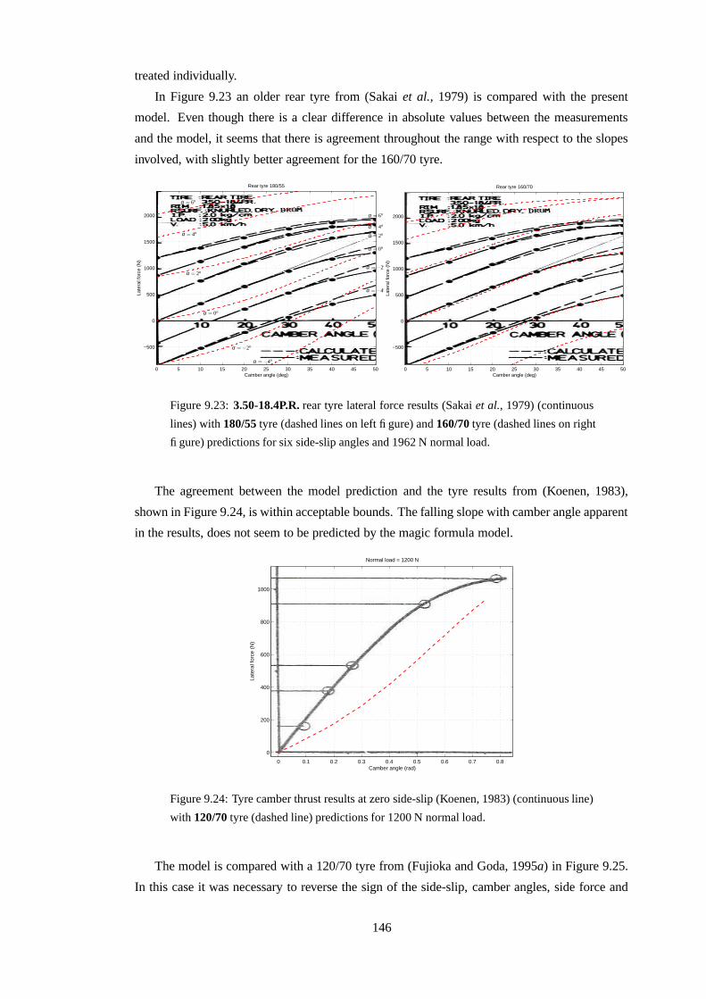
treated individually.
In Figure 9.23 an older rear tyre from (Sakai et al., 1979) is compared with the present
model. Even though there is a clear difference in absolute values between the measurements
and the model, it seems that there is agreement throughout the range with respect to the slopes
involved, with slightly better agreement for the 160/70 tyre.
Camber angle (deg)
Late
ral f
orce
(N
)
Rear tyre 180/55
0 5 10 15 20 25 30 35 40 45 50
−500
0
500
1000
1500
2000
α = −4o
α = −2o
α = 0o
α = 2o
α = 4o
α = 6o
α = −4o
α = −2o
α = 0o
α = 2o
α = 4o
α = 6o
Camber angle (deg)
Late
ral f
orce
(N
)
Rear tyre 160/70
0 5 10 15 20 25 30 35 40 45 50
−500
0
500
1000
1500
2000
Figure 9.23: 3.50-18.4P.R. rear tyre lateral force results (Sakai et al., 1979) (continuous
lines) with 180/55 tyre (dashed lines on left figure) and 160/70 tyre (dashed lines on right
figure) predictions for six side-slip angles and 1962 N normal load.
The agreement between the model prediction and the tyre results from (Koenen, 1983),
shown in Figure 9.24, is within acceptable bounds. The falling slope with camber angle apparent
in the results, does not seem to be predicted by the magic formula model.
Camber angle (rad)
Late
ral f
orce
(N
)
Normal load = 1200 N
0 0.1 0.2 0.3 0.4 0.5 0.6 0.7 0.8
0
200
400
600
800
1000
Figure 9.24: Tyre camber thrust results at zero side-slip (Koenen, 1983) (continuous line)
with 120/70 tyre (dashed line) predictions for 1200 N normal load.
The model is compared with a 120/70 tyre from (Fujioka and Goda, 1995a) in Figure 9.25.
In this case it was necessary to reverse the sign of the side-slip, camber angles, side force and
146
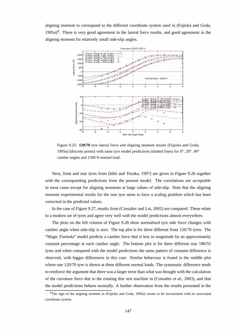
aligning moment to correspond to the different coordinate system used in (Fujioka and Goda,
1995a)8 . There is very good agreement in the lateral force results, and good agreement in the
aligning moment for relatively small side-slip angles.
Late
ral f
orce
(N
)
Front tyre (120/70 ZR17)
Normal load = 1500 N
−8 −6 −4 −2 0 2 4 6 8−1500
−1000
−500
0
500
1000
1500
2000
Side−slip angle (deg)
Alig
ning
mom
ent (
Nm
)
−8 −6 −4 −2 0 2 4 6 8−60
−40
−20
0
20
Figure 9.25: 120/70 tyre lateral force and aligning moment results (Fujioka and Goda,
1995a) (discrete points) with same tyre model predictions (dashed lines) for 0o, 20o, 40o
camber angles and 1500 N normal load.
Next, front and rear tyres from (Ishii and Tezuka, 1997) are given in Figure 9.26 together
with the corresponding predictions from the present model. The correlations are acceptable
in most cases except for aligning moments at large values of side-slip. Note that the aligning
moment experimental results for the rear tyre seem to have a scaling problem which has been
corrected in the predicted values.
In the case of Figure 9.27, results from (Cossalter and Lot, 2002) are compared. These relate
to a modern set of tyres and agree very well with the model predictions almost everywhere.
The plots on the left column of Figure 9.28 show normalised tyre side force changes with
camber angle when side-slip is zero. The top plot is for three different front 120/70 tyres. The
“Magic Formula” model predicts a camber force that is less in magnitude by an approximately
constant percentage at each camber angle. The bottom plot is for three different rear 180/55
tyres and when compared with the model predictions the same pattern of constant difference is
observed, with bigger differences in this case. Similar behaviour is found in the middle plot
where one 120/70 tyre is shown at three different normal loads. The systematic difference tends
to reinforce the argument that there was a larger error than what was thought with the calculation
of the curvature force due to the rotating disc test machine in (Cossalter et al., 2003), and that
the model predictions behave normally. A further observation from the results presented in the
8The sign of the aligning moment in (Fujioka and Goda, 1995a) seems to be inconsistent with its associated
coordinate system.
147
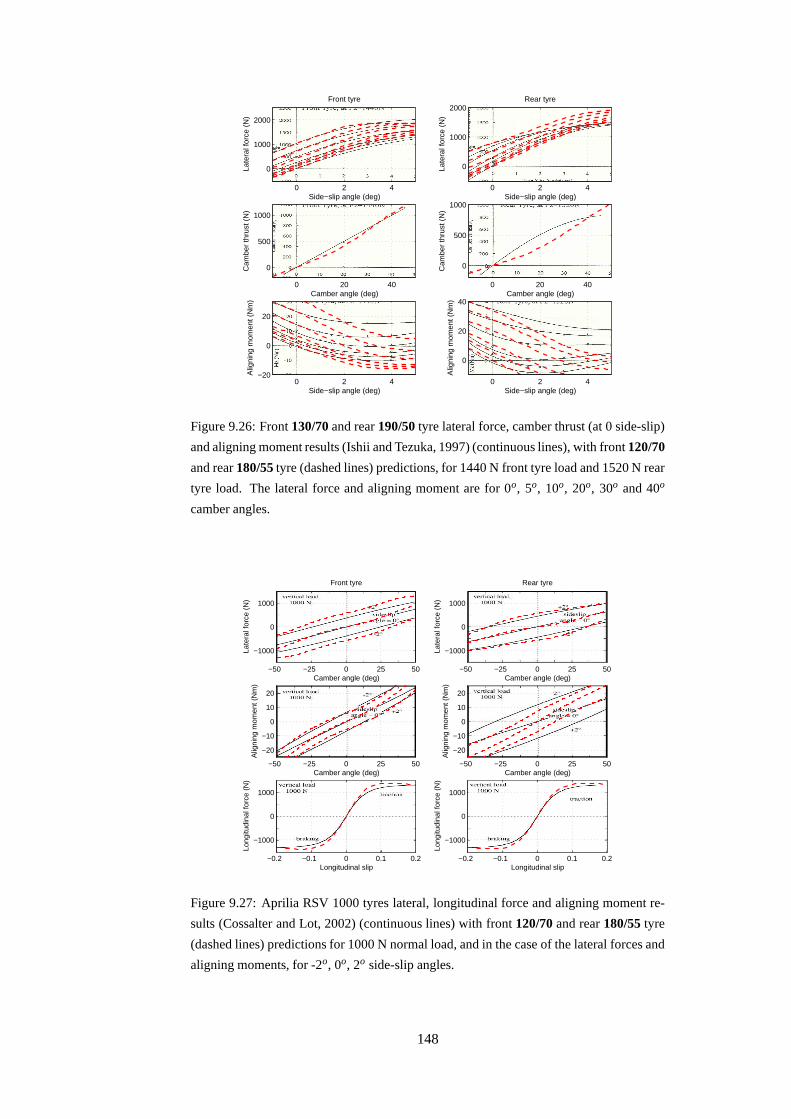
Side−slip angle (deg)
Late
ral f
orce
(N
)
Rear tyre
0 2 4
0
1000
2000
Camber angle (deg)
Cam
ber
thru
st (
N)
0 20 40
0
500
1000
Side−slip angle (deg)
Alig
ning
mom
ent (
Nm
)
0 2 4
0
20
40
Side−slip angle (deg)
Late
ral f
orce
(N
)
Front tyre
0 2 4
0
1000
2000
Camber angle (deg)
Cam
ber
thru
st (
N)
0 20 40
0
500
1000
Side−slip angle (deg)
Alig
ning
mom
ent (
Nm
)
0 2 4−20
0
20
Figure 9.26: Front 130/70 and rear 190/50 tyre lateral force, camber thrust (at 0 side-slip)
and aligning moment results (Ishii and Tezuka, 1997) (continuous lines), with front 120/70
and rear 180/55 tyre (dashed lines) predictions, for 1440 N front tyre load and 1520 N rear
tyre load. The lateral force and aligning moment are for 0o, 5o, 10o, 20o, 30o and 40o
camber angles.
Camber angle (deg)
Late
ral f
orce
(N
)
Rear tyre
−50 −25 0 25 50
−1000
0
1000
Longitudinal slip
Long
itudi
nal f
orce
(N
)
−0.2 −0.1 0 0.1 0.2
−1000
0
1000
Camber angle (deg)
Alig
ning
mom
ent (
Nm
)
−50 −25 0 25 50
−20
−10
0
10
20
Camber angle (deg)
Late
ral f
orce
(N
)
Front tyre
−50 −25 0 25 50
−1000
0
1000
Longitudinal slip
Long
itudi
nal f
orce
(N
)
−0.2 −0.1 0 0.1 0.2
−1000
0
1000
Camber angle (deg)
Alig
ning
mom
ent (
Nm
)
−50 −25 0 25 50
−20
−10
0
10
20
Figure 9.27: Aprilia RSV 1000 tyres lateral, longitudinal force and aligning moment re-
sults (Cossalter and Lot, 2002) (continuous lines) with front 120/70 and rear 180/55 tyre
(dashed lines) predictions for 1000 N normal load, and in the case of the lateral forces and
aligning moments, for -2o, 0o, 2o side-slip angles.
148
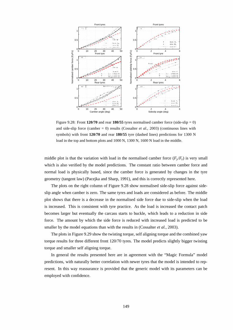
Front tyres
0 10 20 30 40 500
0.5
1
Front tyres
0 2 4 60
0.5
1
Nor
mal
ised
cam
ber
forc
e (F
y/F
z)
Front tyre
0 10 20 30 40 500
0.5
1
Nor
mal
ised
sid
elsl
ip fo
rce
(Fy/
Fz)
Front tyre
0 2 4 60
0.5
1
Camber angle (deg)
Rear tyres
0 10 20 30 40 500
0.5
1
Sideslip angle (deg)
Rear tyres
0 2 4 60
0.5
1
Figure 9.28: Front 120/70 and rear 180/55 tyres normalised camber force (side-slip = 0)
and side-slip force (camber = 0) results (Cossalter et al., 2003) (continuous lines with
symbols) with front 120/70 and rear 180/55 tyre (dashed lines) predictions for 1300 N
load in the top and bottom plots and 1000 N, 1300 N, 1600 N load in the middle.
middle plot is that the variation with load in the normalised camber force (Fy/Fz) is very small
which is also verified by the model predictions. The constant ratio between camber force and
normal load is physically based, since the camber force is generated by changes in the tyre
geometry (tangent law) (Pacejka and Sharp, 1991), and this is correctly represented here.
The plots on the right column of Figure 9.28 show normalised side-slip force against side-
slip angle when camber is zero. The same tyres and loads are considered as before. The middle
plot shows that there is a decrease in the normalised side force due to side-slip when the load
is increased. This is consistent with tyre practice. As the load is increased the contact patch
becomes larger but eventually the carcass starts to buckle, which leads to a reduction in side
force. The amount by which the side force is reduced with increased load is predicted to be
smaller by the model equations than with the results in (Cossalter et al., 2003).
The plots in Figure 9.29 show the twisting torque, self aligning torque and the combined yaw
torque results for three different front 120/70 tyres. The model predicts slightly bigger twisting
torque and smaller self aligning torque.
In general the results presented here are in agreement with the “Magic Formula” model
predictions, with naturally better correlation with newer tyres that the model is intended to rep-
resent. In this way reassurance is provided that the generic model with its parameters can be
employed with confidence.
149
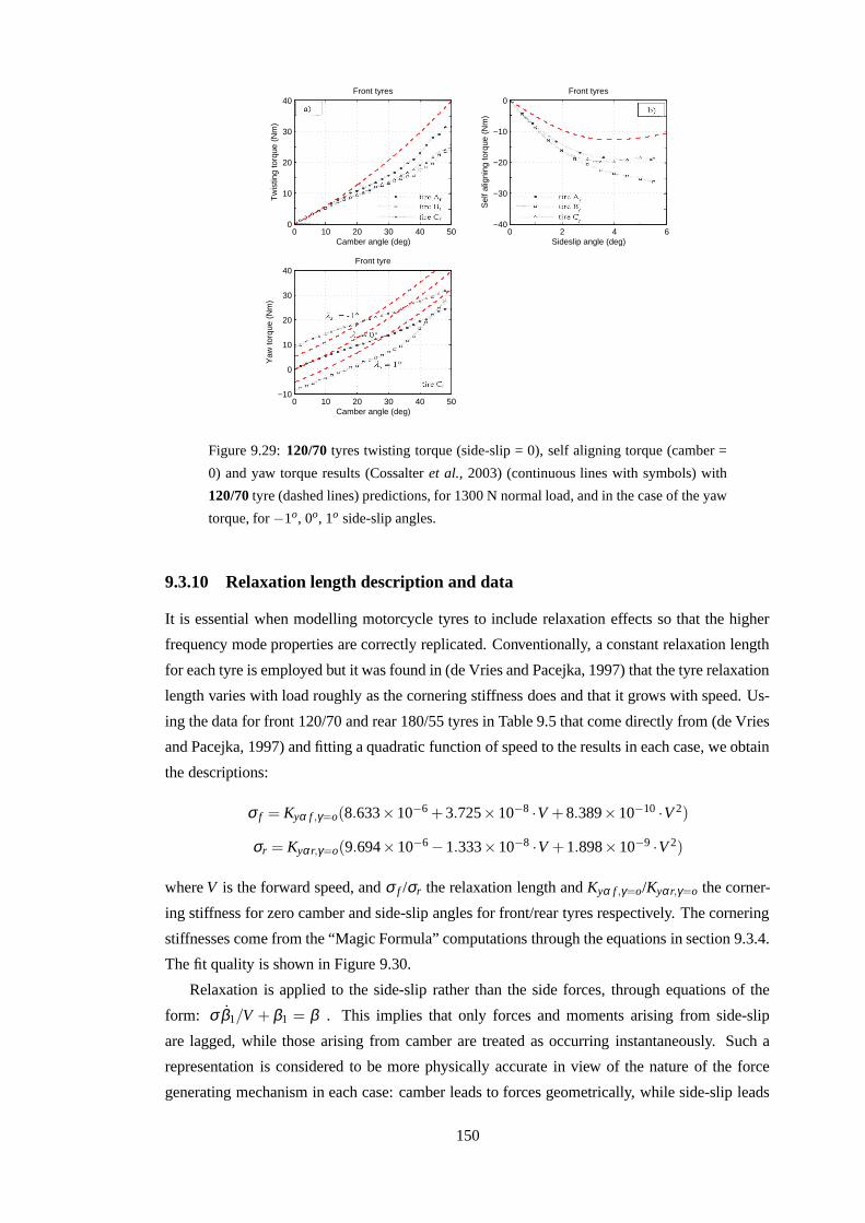
Camber angle (deg)
Tw
istin
g to
rque
(N
m)
Front tyres
0 10 20 30 40 500
10
20
30
40
Sideslip angle (deg)
Sel
f alig
ning
torq
ue (
Nm
)
Front tyres
0 2 4 6−40
−30
−20
−10
0
Camber angle (deg)
Yaw
torq
ue (
Nm
)Front tyre
0 10 20 30 40 50−10
0
10
20
30
40
Figure 9.29: 120/70 tyres twisting torque (side-slip = 0), self aligning torque (camber =
0) and yaw torque results (Cossalter et al., 2003) (continuous lines with symbols) with
120/70 tyre (dashed lines) predictions, for 1300 N normal load, and in the case of the yaw
torque, for −1o, 0o, 1o side-slip angles.
9.3.10 Relaxation length description and data
It is essential when modelling motorcycle tyres to include relaxation effects so that the higher
frequency mode properties are correctly replicated. Conventionally, a constant relaxation length
for each tyre is employed but it was found in (de Vries and Pacejka, 1997) that the tyre relaxation
length varies with load roughly as the cornering stiffness does and that it grows with speed. Us-
ing the data for front 120/70 and rear 180/55 tyres in Table 9.5 that come directly from (de Vries
and Pacejka, 1997) and fitting a quadratic function of speed to the results in each case, we obtain
the descriptions:
σ f = Kyα f ,γ=o(8.633×10⁻⁶ +3.725×10⁻⁸ ·V +8.389×10⁻¹⁰ ·V 2)
σr = Kyαr,γ=o(9.694×10⁻⁶ −1.333×10⁻⁸ ·V +1.898×10⁻⁹ ·V 2)
where V is the forward speed, and σ f /σr the relaxation length and Kyα f ,γ=o/Kyαr,γ=o the corner-
ing stiffness for zero camber and side-slip angles for front/rear tyres respectively. The cornering
stiffnesses come from the “Magic Formula” computations through the equations in section 9.3.4.
The fit quality is shown in Figure 9.30.
Relaxation is applied to the side-slip rather than the side forces, through equations of the
form: σβ1/V + β1 = β . This implies that only forces and moments arising from side-slip
are lagged, while those arising from camber are treated as occurring instantaneously. Such a
representation is considered to be more physically accurate in view of the nature of the force
generating mechanism in each case: camber leads to forces geometrically, while side-slip leads
150
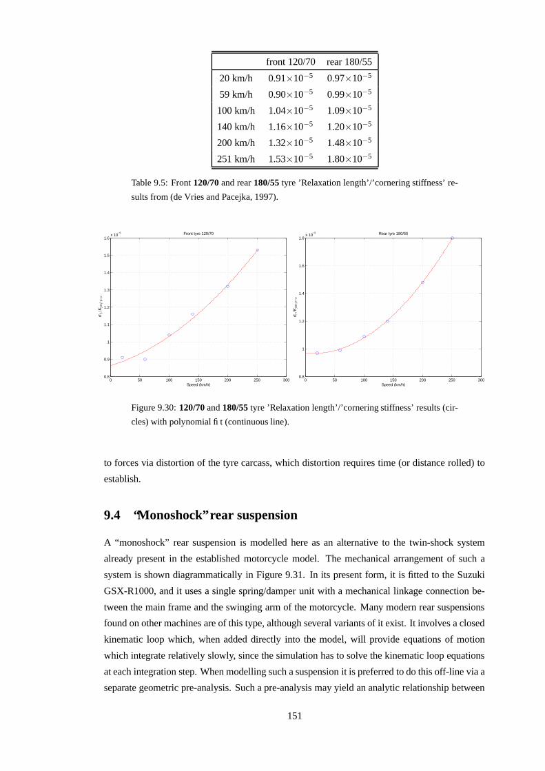
front 120/70 rear 180/55
20 km/h 0.91×10⁻⁵ 0.97×10⁻⁵
59 km/h 0.90×10⁻⁵ 0.99×10⁻⁵
100 km/h 1.04×10⁻⁵ 1.09×10⁻⁵
140 km/h 1.16×10⁻⁵ 1.20×10⁻⁵
200 km/h 1.32×10⁻⁵ 1.48×10⁻⁵
251 km/h 1.53×10⁻⁵ 1.80×10⁻⁵
Table 9.5: Front 120/70 and rear 180/55 tyre ’Relaxation length’/’cornering stiffness’ re-
sults from (de Vries and Pacejka, 1997).
0 50 100 150 200 250 3000.8
0.9
1
1.1
1.2
1.3
1.4
1.5
1.6x 10
−5
Speed (km/h)
Front tyre 120/70
σf/
Kyα
f,γ=
o
0 50 100 150 200 250 3000.8
1
1.2
1.4
1.6
1.8x 10
−5
Speed (km/h)
Rear tyre 180/55
σ r/K
yαr,
γ=o
Figure 9.30: 120/70 and 180/55 tyre ’Relaxation length’/’cornering stiffness’ results (cir-
cles) with polynomial fit (continuous line).
to forces via distortion of the tyre carcass, which distortion requires time (or distance rolled) to
establish.
9.4 “Monoshock” rear suspension
A “monoshock” rear suspension is modelled here as an alternative to the twin-shock system
already present in the established motorcycle model. The mechanical arrangement of such a
system is shown diagrammatically in Figure 9.31. In its present form, it is fitted to the Suzuki
GSX-R1000, and it uses a single spring/damper unit with a mechanical linkage connection be-
tween the main frame and the swinging arm of the motorcycle. Many modern rear suspensions
found on other machines are of this type, although several variants of it exist. It involves a closed
kinematic loop which, when added directly into the model, will provide equations of motion
which integrate relatively slowly, since the simulation has to solve the kinematic loop equations
at each integration step. When modelling such a suspension it is preferred to do this off-line via a
separate geometric pre-analysis. Such a pre-analysis may yield an analytic relationship between
151

x
z
PSfrag replacements
ppp777
ppp11
ppp13
ppp19
ppp20
ppp21
ppp22
lll111
lll222
lll333
lll444
lll
ζ
θθc
δφ0
Figure 9.31: Geometry of monoshock suspension arrangement on GSX-R1000 motorcy-
cle.
the swinging arm angle change and angular speed, and the moment of the spring/damper force
about the swinging arm pivot, which is then added directly in the motorcycle model building.
The analysis follows.
Points p11, p13 and p19 are fixed to the main frame. l1, l4 and φo are dimensions of the
swinging link and l2 the length of the pull rod. l3 is a fixed length in the swinging arm. The
spring/damper unit is of variable length l. θ is the sum of the angle of the swinging arm to the
horizontal x-axis and the fixed angle θc, which is the angle of the line connecting points p11 and
p22 to the horizontal in the nominal configuration (the swinging arm is not necessarily horizontal
in the nominal configuration). δ and ζ are angles to the horizontal for the swinging link and pull
rod respectively. Traversing the loop p19-p20-p22-p11-p19, both x and z displacements are nil,
since we end where we begin. Therefore:
x11 − x19 − l3 cos θ + l2 cosζ + l1 cos δ = 0
and
z11 − z19 + l3 sinθ + l2 sinζ − l1 sinδ = 0
Forming l22 as (l2
2 sin2 ζ + l22 cos2 ζ ) and substituting:
c1 = −x11 + x19 + l3 cos θ
and
c2 = −z11 + z19 − l3 sinθ
152
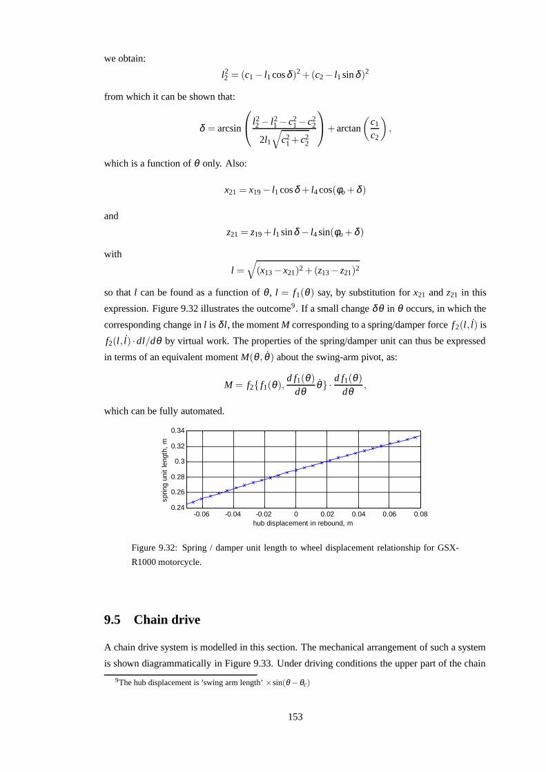
we obtain:
l22 = (c1 − l1 cosδ )2 +(c2 − l1 sin δ )2
from which it can be shown that:
δ = arcsin
l22 − l2
1 − c21 − c2
2
2l1√
c21 + c2
2
+ arctan
(
c1
c2
)
,
which is a function of θ only. Also:
x21 = x19 − l1 cosδ + l4 cos(φo +δ )
and
z21 = z19 + l1 sinδ − l4 sin(φo +δ )
with
l =√
(x13 − x21)2 +(z13 − z21)2
so that l can be found as a function of θ , l = f1(θ) say, by substitution for x21 and z21 in this
expression. Figure 9.32 illustrates the outcome9. If a small change δθ in θ occurs, in which the
corresponding change in l is δ l, the moment M corresponding to a spring/damper force f2(l, l) is
f2(l, l) ·dl/dθ by virtual work. The properties of the spring/damper unit can thus be expressed
in terms of an equivalent moment M(θ , θ ) about the swing-arm pivot, as:
M = f2{ f1(θ),d f1(θ)
dθθ} · d f1(θ)
dθ,
which can be fully automated.
-0.06 -0.04 -0.02 0 0.02 0.04 0.06 0.080.24
0.26
0.28
0.3
0.32
0.34
hub displacement in rebound, m
sprin
g un
it le
ngth
, m
Figure 9.32: Spring / damper unit length to wheel displacement relationship for GSX-
R1000 motorcycle.
9.5 Chain drive
A chain drive system is modelled in this section. The mechanical arrangement of such a system
is shown diagrammatically in Figure 9.33. Under driving conditions the upper part of the chain
9The hub displacement is ’swing arm length’ ×sin(θ −θc)
153
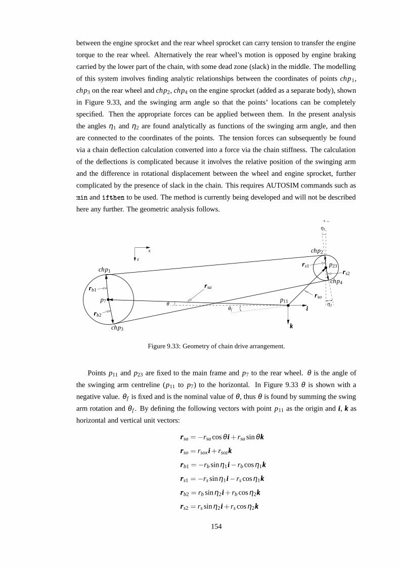
between the engine sprocket and the rear wheel sprocket can carry tension to transfer the engine
torque to the rear wheel. Alternatively the rear wheel’s motion is opposed by engine braking
carried by the lower part of the chain, with some dead zone (slack) in the middle. The modelling
of this system involves finding analytic relationships between the coordinates of points chp1,
chp3 on the rear wheel and chp2, chp4 on the engine sprocket (added as a separate body), shown
in Figure 9.33, and the swinging arm angle so that the points’ locations can be completely
specified. Then the appropriate forces can be applied between them. In the present analysis
the angles η1 and η2 are found analytically as functions of the swinging arm angle, and then
are connected to the coordinates of the points. The tension forces can subsequently be found
via a chain deflection calculation converted into a force via the chain stiffness. The calculation
of the deflections is complicated because it involves the relative position of the swinging arm
and the difference in rotational displacement between the wheel and engine sprocket, further
complicated by the presence of slack in the chain. This requires AUTOSIM commands such as� �
� and� � � � � � to be used. The method is currently being developed and will not be described
here any further. The geometric analysis follows.
PSfrag replacements
rrrsarrrb1
rrrb2
rrrso
rrrs1rrrs2
η1
η2θθ f
chp1
chp2
chp3
chp4
iii
kkk
p7 p11
p23
x
z
+ –
Figure 9.33: Geometry of chain drive arrangement.
Points p11 and p23 are fixed to the main frame and p7 to the rear wheel. θ is the angle of
the swinging arm centreline (p11 to p7) to the horizontal. In Figure 9.33 θ is shown with a
negative value. θ f is fixed and is the nominal value of θ , thus θ is found by summing the swing
arm rotation and θ f . By defining the following vectors with point p11 as the origin and iii, kkk as
horizontal and vertical unit vectors:
rrrsa = −rsa cosθ iii + rsa sinθkkk
rrrso = rsoxiii+ rsozkkk
rrrb1 = −rb sinη1iii− rb cosη1kkk
rrrs1 = −rs sinη1iii− rs cosη1kkk
rrrb2 = rb sinη2iii+ rb cos η2kkk
rrrs2 = rs sinη2iii+ rs cosη2kkk
154
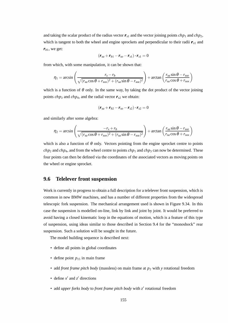
and taking the scalar product of the radius vector rrrs1 and the vector joining points chp1 and chp2,
which is tangent to both the wheel and engine sprockets and perpendicular to their radii rrrs1 and
rrrb1, we get:
(rrrsa + rrrb1 − rrrso − rrrs1) ··· rrrs1 = 0
from which, with some manipulation, it can be shown that:
η1 = arcsin
(
rs − rb√
(rsa cosθ + rsox)2 +(rsa sinθ − rsoz)2
)
+ arctan
(
rsa sinθ − rsoz
rsa cosθ + rsox
)
which is a function of θ only. In the same way, by taking the dot product of the vector joining
points chp3 and chp4, and the radial vector rrrs2 we obtain:
(rrrsa + rrrb2 − rrrso − rrrs2) ··· rrrs2 = 0
and similarly after some algebra:
η2 = arcsin
(
−rs + rb√
(rsa cosθ + rsox)2 +(rsa sinθ − rsoz)2
)
+ arctan
(
rsa sinθ − rsoz
rsa cosθ + rsox
)
which is also a function of θ only. Vectors pointing from the engine sprocket centre to points
chp2 and chp4, and from the wheel centre to points chp1 and chp3 can now be determined. These
four points can then be defined via the coordinates of the associated vectors as moving points on
the wheel or engine sprocket.
9.6 Telelever front suspension
Work is currently in progress to obtain a full description for a telelever front suspension, which is
common in new BMW machines, and has a number of different properties from the widespread
telescopic fork suspension. The mechanical arrangement used is shown in Figure 9.34. In this
case the suspension is modelled on-line, link by link and joint by joint. It would be preferred to
avoid having a closed kinematic loop in the equations of motion, which is a feature of this type
of suspension, using ideas similar to those described in Section 9.4 for the “monoshock” rear
suspension. Such a solution will be sought in the future.
The model building sequence is described next:
• define all points in global coordinates
• define point p15 in main frame
• add front frame pitch body (massless) on main frame at p2 with y rotational freedom
• define x′ and z′ directions
• add upper forks body to front frame pitch body with z′ rotational freedom
155
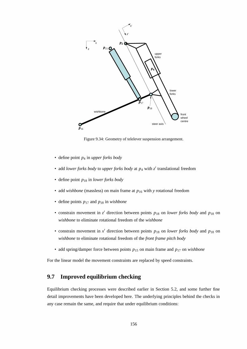
upperforks
lowerforks
frontwheelcentre
z
x
steer axis
wishbone
x’
z’
PSfrag replacements
ppp222
ppp444
ppp15
ppp16
ppp17
ppp18
Figure 9.34: Geometry of telelever suspension arrangement.
• define point p4 in upper forks body
• add lower forks body to upper forks body at p4 with z′ translational freedom
• define point p18 in lower forks body
• add wishbone (massless) on main frame at p16 with y rotational freedom
• define points p17 and p18 in wishbone
• constrain movement in z′ direction between points p18 on lower forks body and p18 on
wishbone to eliminate rotational freedom of the wishbone
• constrain movement in x′ direction between points p18 on lower forks body and p18 on
wishbone to eliminate rotational freedom of the front frame pitch body
• add spring/damper force between points p15 on main frame and p17 on wishbone
For the linear model the movement constraints are replaced by speed constraints.
9.7 Improved equilibrium checking
Equilibrium checking processes were described earlier in Section 5.2, and some further fine
detail improvements have been developed here. The underlying principles behind the checks in
any case remain the same, and require that under equilibrium conditions:
156
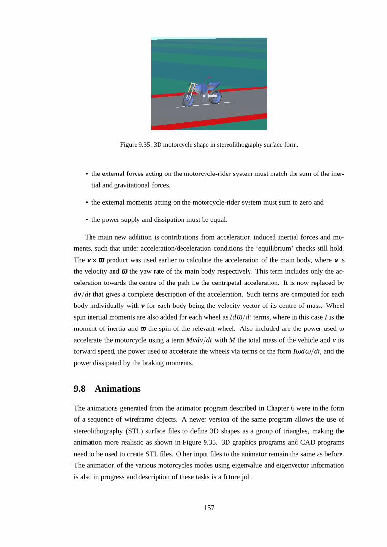
Figure 9.35: 3D motorcycle shape in stereolithography surface form.
• the external forces acting on the motorcycle-rider system must match the sum of the iner-
tial and gravitational forces,
• the external moments acting on the motorcycle-rider system must sum to zero and
• the power supply and dissipation must be equal.
The main new addition is contributions from acceleration induced inertial forces and mo-
ments, such that under acceleration/deceleration conditions the ‘equilibrium’ checks still hold.
The vvv×××ωωω product was used earlier to calculate the acceleration of the main body, where vvv is
the velocity and ωωω the yaw rate of the main body respectively. This term includes only the ac-
celeration towards the centre of the path i.e the centripetal acceleration. It is now replaced by
dvvv/dt that gives a complete description of the acceleration. Such terms are computed for each
body individually with vvv for each body being the velocity vector of its centre of mass. Wheel
spin inertial moments are also added for each wheel as Idω/dt terms, where in this case I is the
moment of inertia and ω the spin of the relevant wheel. Also included are the power used to
accelerate the motorcycle using a term Mvdv/dt with M the total mass of the vehicle and v its
forward speed, the power used to accelerate the wheels via terms of the form Iωdω/dt, and the
power dissipated by the braking moments.
9.8 Animations
The animations generated from the animator program described in Chapter 6 were in the form
of a sequence of wireframe objects. A newer version of the same program allows the use of
stereolithography (STL) surface files to define 3D shapes as a group of triangles, making the
animation more realistic as shown in Figure 9.35. 3D graphics programs and CAD programs
need to be used to create STL files. Other input files to the animator remain the same as before.
The animation of the various motorcycles modes using eigenvalue and eigenvector information
is also in progress and description of these tasks is a future job.
157
Part V
Conclusions and Future Work
158
Chapter 10
Conclusions
The use of automated methods for generating equations of motion and analysing motorcycle
dynamics has been demonstrated. In particular it has been shown that the hand derived results
in (Sharp, 1971, 1994b) can be reproduced by the multi-body modelling code AUTOSIM. As
is the case with many nonlinear systems, local stability is investigated via the eigenvalues of
linearised models that are associated with equilibrium points of the nonlinear system. The full
nonlinear equations of motion in each case are obtained in FORTRAN or C code that is used
to generate time histories, and the linearised state-space model is obtained in symbolic form as
a MATLAB m-file. The employment of feedback controllers is necessary to establish specified
straight running or cornering equilibrium states prior to testing the stability. A typical local
stability study requires the importation of quasi-steady time histories from the nonlinear model
to the symbolic linearised equations of motion.
A more comprehensive model has also been presented, capable of more general equilibrium
conditions, acceleration/deceleration conditions and road forcing on the wheels. The relevant
account given here is based on previous work from (Sharp and Limebeer, 2001). There is novelty
in the development of animation runs with the same model.
The modern theoretical techniques developed have been employed to investigate the be-
haviour of motorcycles under acceleration and deceleration. Extensive use has been made of
both nonlinear and linearised models. Control systems have been used to control the motorcycle
drive and braking systems in order that the machine maintains preset rates of acceleration or
deceleration. The results show that the wobble mode damping of a motorcycle is significantly
reduced when the machine is descending an incline or braking on a level surface. Conversely,
the wobble mode is substantially stabilised when the machine is ascending an incline at constant
speed or accelerating on a level surface. Ascending, descending inclines, acceleration and de-
celeration appear to have very little influence on the damping or frequency of the weave mode.
(Sharp, 1976b) reported that acceleration can reduce weave mode damping by a large amount
and that the weave and wobble modes can lose their identities because of the narrowing of the
frequency gap between these modes. Neither of these observations were predicted in this study
which reinforces the idea that the model and ideas employed in (Sharp, 1976b) were too simpli-
159
fied for the intended purpose.
The known problems to do with rear tyre adhesion in heavy rear-wheel-dominated braking
situations have also been exposed by nonlinear simulations. The analysis has quantified the
transfer of normal tyre loading to the front tyre under heavy braking, which implies that the rear
tyre cannot perform its task under such conditions. If an attempt is made to slow the machine
using rear-wheel-dominated braking, it very likely that the rear tyre will go into a slide, causing
an irrecoverable loss of control. The aerodynamic drag does some of the braking and reduces
these difficulties at high speeds.
Theoretical analysis with the use of the techniques developed has also been carried out to
examine the behaviour of motorcycles under road forcing conditions. The results presented show
that under cornering, regular low-amplitude road undulations can be a source of considerable
difficulty to motorcycle riders. At low machine speeds the wobble and front suspension pitch
modes are likely to respond vigorously to resonant forcing, while at higher speeds, the weave
and front wheel hop modes are similarly affected. The vigour of the oscillations is related to the
amount of damping present in each mode, with low damping factors leading to correspondingly
high peak magnification factors.
The individual contributions to these resonances made by each of the two road wheels have
been studied. The results show that the wobble and front wheel hop resonance peaks are “front
wheel dominated”. In other words, difficulties with these modes are likely to be caused by the
design and set up of the front of the machine. The same is true, but to a lesser extent, in the case
of the front suspension pitch mode. In contrast, the weave mode resonance peak involves the
road forcing to both wheels in almost equal measure. As a consequence, weave related problems
appear to be more difficult to isolate and remove.
As might be anticipated, the vulnerability of the wobble mode response to road forcing is
decreased markedly by an effective steering damper, but changes to the suspension dampers
are ineffectual. The front suspension pitch mode resonance is sensitive to the front suspension
damping, but is insensitive to the rear suspension and steering damping. The weave mode res-
onant response appears to be reduced by increasing the front damping, but it is made larger by
increasing the rear suspension and steering damper settings. Increasing the front suspension
damping reduces the front wheel hop resonance peak, but this peak does not respond to changes
in steering damping, or rear suspension damper settings.
It has also been shown that light riders are more likely to suffer from road forced resonant
weave oscillations than are heavy ones, as has been observed in practice (Farr, 1997a) and on
the video tape (Dunlop, c1977). The results indicate also that the peak gains associated with
the weave mode are brought down by moving the rider upper body mass forwards and upwards.
There is not sufficient practical evidence at the moment to indicate whether or not these findings
coincide with experience. From a safety point of view, a worrying feature of the road profile
induced oscillations is the tendency of the uncontrolled machine to “sit up” and run wide. This
aspect of the machine behaviour can be seen on the video tape (Duke Marketing Ltd, 1999) in
the case of a high-speed weave accident.
160
The work reported here has a number of practical consequences. It appears to provide an
explanation for a class of single vehicle loss-of-rider-control accidents reported in the popular
literature, and it helps to explain why motorcycles that behave perfectly well for long periods
can suddenly suffer serious and dangerous oscillation problems. Such oscillations are likely to
be difficult to reproduce and study in practice, because they occur under a rare combination of
running conditions, characterised by the machine speed, the lean angle, the rider’s mass and
posture, and the road profile wavelength. The safety of the rider is also an issue. The kind
of theoretical analysis presented here provides a safe and economical way for reproducing and
studying these dangerous oscillatory phenomena associated with motorcycles, and can easily be
used by motorcycle manufacturers to determine “worst case” operating conditions for their new
products.
New work has also been started and described here, relating to modelling improvements
to the already advanced motorcycle model described earlier in this thesis. The tyre model, in
particular, has been fully developed to provide a generic description of a set of modern high
performance motorcycle tyres with a wide range of validity. The basis for the shear force and
moment description is the powerful Magic Formula method, for which parameters have been de-
rived from recent published tyre results. The tyre relaxation properties have also been updated,
and the tyre-road contact geometry has been adapted to correspond to the geometry of a wide
tyre, as opposed to the previously infinitely thin tyre assumed. Improved equilibrium checking
procedures have also been developed. A monoshock rear suspension has been described through
a separate off-line geometric analysis. Significant progress has been made in modelling other
parts of the motorcycle design–chain drive, front telelever suspension–, and in obtaining a com-
plete parametric description of a contemporary, high performance motorcycle, although further
work is required to complete these tasks.
161
Chapter 11
Future Work
The immediate work that needs to be completed in the future involves the pending modelling
improvements described earlier and the parametric description of a modern sports bike. The
chain drive and telelever front suspension, in particular, need to be finalised and the remaining
unknown parameters to be measured. More advanced animations, that involve the use of eigen-
value and eigenvector information from linearised models, can show the various normal modes
of the motorcycle in a 3-dimensional form. Further work is required to complete such animation
tasks or animations of any other general motion of the motorcycle with the newly developed
solid object form.
In the improved motorcycle model, a first order relaxation model has been used to capture
the transient behaviour of the tyre. Although this is adequate for the present purposes it might
be advantageous, in other circumstances, to model the tyre carcass as a rigid ring, that correctly
represents the tyre behaviour for a larger range of frequencies. This feature when included
complicates the tyre model substantially and the benefits to be gained have to outweigh the
increase in complexity, if it is to be used.
A preliminary time domain study of motion simulations under resonance conditions has been
presented earlier. It has shown the existence of interesting and essentially nonlinear phenom-
ena, that seem to conform with practical experience. The task of understanding these nonlinear
phenomena has been undertaken in a separate project and time-frequency signal processing tech-
niques have been employed in an attempt to detect super-harmonic or sub-harmonic excitations
of the resonant motorcycle modes. The results appear to indicate that road forcing induced oscil-
lations are mainly explained by the linear theory presented in this thesis and the use of nonlinear
techniques is not necessary, but further investigation is clearly required before anything can be
said with certainty. Bifurcation theory can also help to further examine nonlinear stability, par-
ticularly with respect to the not so well understood high speed wobble, commonly known as a
“tank slapper”.
The completed representation of a modern high performance machine will be used to de-
termine steady turning, stability, response and parameter sensitivity data to be compared with
older information and determine to what extent it remains valid in order to acquire a better un-
162
derstanding of modern machines. In addition, the linearised version of the motorcycle model
can be used to develop the rider’s feedback stabilisation and path following response via linear
optimal preview steering and rider lean control.
163
Part VI
Appendices
164
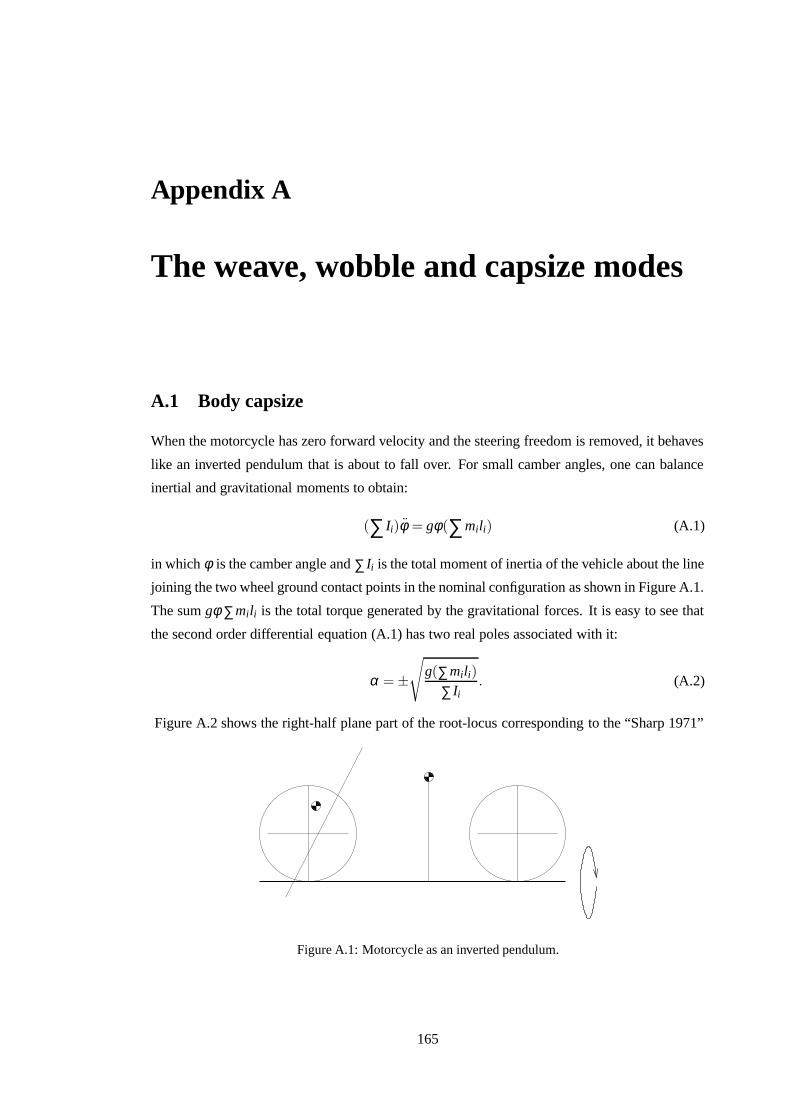
Appendix A
The weave, wobble and capsize modes
A.1 Body capsize
When the motorcycle has zero forward velocity and the steering freedom is removed, it behaves
like an inverted pendulum that is about to fall over. For small camber angles, one can balance
inertial and gravitational moments to obtain:
(∑ Ii)φ = gφ(∑mili) (A.1)
in which φ is the camber angle and ∑ Ii is the total moment of inertia of the vehicle about the line
joining the two wheel ground contact points in the nominal configuration as shown in Figure A.1.
The sum gφ ∑mili is the total torque generated by the gravitational forces. It is easy to see that
the second order differential equation (A.1) has two real poles associated with it:
α = ±√
g(∑mili)
∑ Ii. (A.2)
Figure A.2 shows the right-half plane part of the root-locus corresponding to the “Sharp 1971”
Figure A.1: Motorcycle as an inverted pendulum.
165
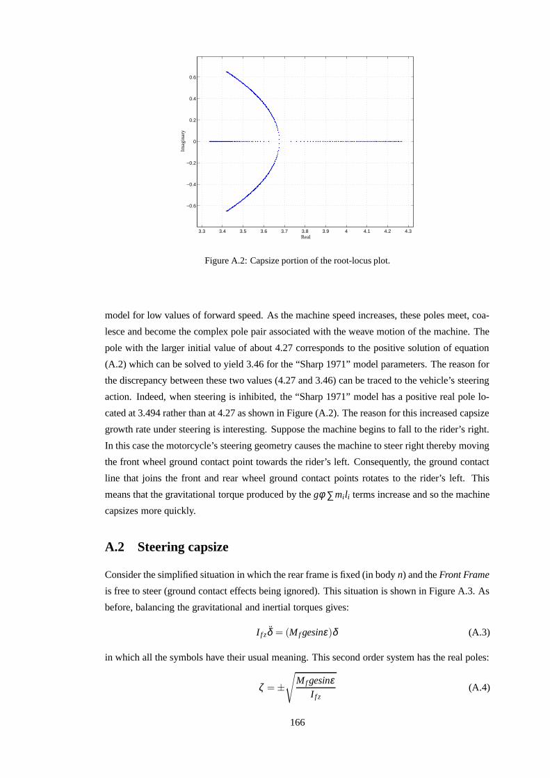
3.3 3.4 3.5 3.6 3.7 3.8 3.9 4 4.1 4.2 4.3
−0.6
−0.4
−0.2
0
0.2
0.4
0.6
PSfrag replacements
Imag
inar
y
Real
Figure A.2: Capsize portion of the root-locus plot.
model for low values of forward speed. As the machine speed increases, these poles meet, coa-
lesce and become the complex pole pair associated with the weave motion of the machine. The
pole with the larger initial value of about 4.27 corresponds to the positive solution of equation
(A.2) which can be solved to yield 3.46 for the “Sharp 1971” model parameters. The reason for
the discrepancy between these two values (4.27 and 3.46) can be traced to the vehicle’s steering
action. Indeed, when steering is inhibited, the “Sharp 1971” model has a positive real pole lo-
cated at 3.494 rather than at 4.27 as shown in Figure (A.2). The reason for this increased capsize
growth rate under steering is interesting. Suppose the machine begins to fall to the rider’s right.
In this case the motorcycle’s steering geometry causes the machine to steer right thereby moving
the front wheel ground contact point towards the rider’s left. Consequently, the ground contact
line that joins the front and rear wheel ground contact points rotates to the rider’s left. This
means that the gravitational torque produced by the gφ ∑mili terms increase and so the machine
capsizes more quickly.
A.2 Steering capsize
Consider the simplified situation in which the rear frame is fixed (in body n) and the Front Frame
is free to steer (ground contact effects being ignored). This situation is shown in Figure A.3. As
before, balancing the gravitational and inertial torques gives:
I f zδ = (M f gesinε)δ (A.3)
in which all the symbols have their usual meaning. This second order system has the real poles:
ζ = ±√
M f gesinεI f z
(A.4)
166
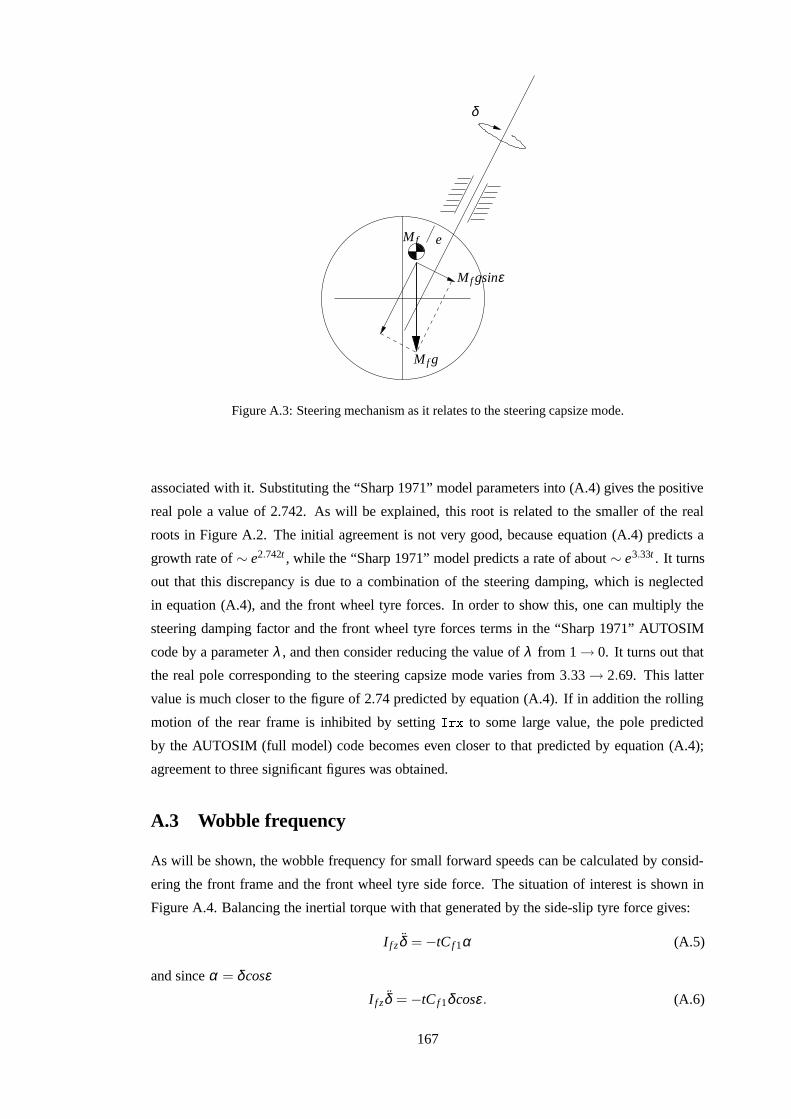
PSfrag replacements
M f e
δ
M f g
M f gsinε
Figure A.3: Steering mechanism as it relates to the steering capsize mode.
associated with it. Substituting the “Sharp 1971” model parameters into (A.4) gives the positive
real pole a value of 2.742. As will be explained, this root is related to the smaller of the real
roots in Figure A.2. The initial agreement is not very good, because equation (A.4) predicts a
growth rate of ∼ e2.742t , while the “Sharp 1971” model predicts a rate of about ∼ e3.33t . It turns
out that this discrepancy is due to a combination of the steering damping, which is neglected
in equation (A.4), and the front wheel tyre forces. In order to show this, one can multiply the
steering damping factor and the front wheel tyre forces terms in the “Sharp 1971” AUTOSIM
code by a parameter λ , and then consider reducing the value of λ from 1 → 0. It turns out that
the real pole corresponding to the steering capsize mode varies from 3.33 → 2.69. This latter
value is much closer to the figure of 2.74 predicted by equation (A.4). If in addition the rolling
motion of the rear frame is inhibited by setting � � � to some large value, the pole predicted
by the AUTOSIM (full model) code becomes even closer to that predicted by equation (A.4);
agreement to three significant figures was obtained.
A.3 Wobble frequency
As will be shown, the wobble frequency for small forward speeds can be calculated by consid-
ering the front frame and the front wheel tyre side force. The situation of interest is shown in
Figure A.4. Balancing the inertial torque with that generated by the side-slip tyre force gives:
I f zδ = −tC f 1α (A.5)
and since α = δcosεI f zδ = −tC f 1δcosε . (A.6)
167
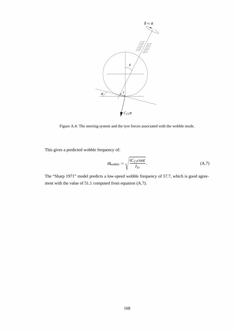
PSfrag replacements
δ ≈ α
ε
t
C f 1α
α
Figure A.4: The steering system and the tyre forces associated with the wobble mode.
This gives a predicted wobble frequency of:
ωwobble =
√
tC f 1cosεI f z
. (A.7)
The “Sharp 1971” model predicts a low-speed wobble frequency of 57.7, which is good agree-
ment with the value of 51.1 computed from equation (A.7).
168
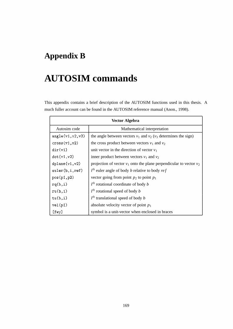
Appendix B
AUTOSIM commands
This appendix contains a brief description of the AUTOSIM functions used in this thesis. A
much fuller account can be found in the AUTOSIM reference manual (Anon., 1998).
Vector Algebra
Autosim code Mathematical interpretation� ? ��� � @ E � @ � � @ � � the angle between vectors v1 and v2 (v3 determines the sign)H ��F � � � @ E � @ � � the cross product between vectors v1 and v2
� � � @ E�� unit vector in the direction of vector v1
�F� � @ E � @ � � inner product between vectors v1 and v2
�G �� � � � @ E � @ � � projection of vector v1 onto the plane perpendicular to vector v2����� � � B � � � � � � � ith euler angle of body b relative to body re f
G�F � � G E ��G � � vector going from point p2 to point p1
� � � B � � � ith rotational coordinate of body b
� ��� B � � � ith rotational speed of body b
� ��� B � � � ith translational speed of body b@ ��� � G E�� absolute velocity vector of point p1� �� A�� symbol is a unit-vector when enclosed in braces
169
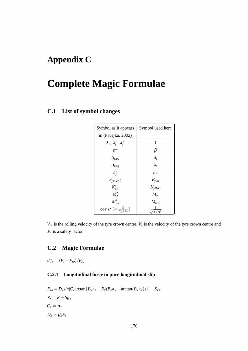
Appendix C
Complete Magic Formulae
C.1 List of symbol changes
Symbol as it appears Symbol used here
in (Pacejka, 2002)
λi, λ ′i , λ ∗
i 1
α∗ βαt,eq λt
αr,eq λr
F ′y Fyt
Fyo,γ=0 Fyoo
K′yα Kyαoo
M′z Mzt
M′zo Mzto
cos′ α (= VcxVc+εV
) 1√1+β 2
Vcx is the rolling velocity of the tyre crown centre, Vc is the velocity of the tyre crown centre and
εV is a safety factor.
C.2 Magic Formulae
d fz = (Fz −Fzo)/Fzo
C.2.1 Longitudinal force in pure longitudinal slip
Fxo = Dxsin[Cxarctan{Bxκx −Ex(Bxκx − arctan(Bxκx))}]+SVx
κx = κ +SHx
Cx = pCx1
Dx = µxFz
170
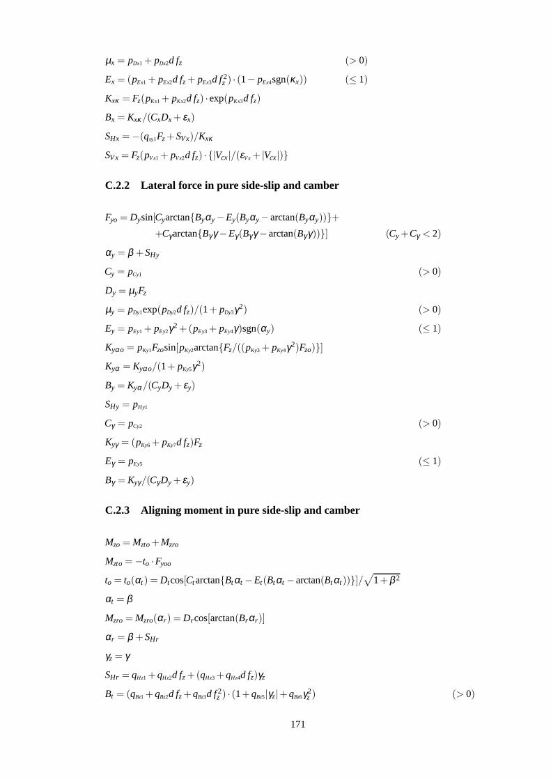
µx = pDx1 + pDx2d fz (> 0)
Ex = (pEx1 + pEx2d fz + pEx3d f 2z ) · (1− pEx4sgn(κx)) (≤ 1)
Kxκ = Fz(pKx1 + pKx2d fz) · exp(pKx3d fz)
Bx = Kxκ/(CxDx + εx)
SHx = −(qsy1Fz +SVx)/Kxκ
SVx = Fz(pV x1 + pVx2d fz) · {|Vcx|/(εV x + |Vcx|)}
C.2.2 Lateral force in pure side-slip and camber
Fyo = Dysin[Cyarctan{Byαy −Ey(Byαy − arctan(Byαy))}++Cγarctan{Bγ γ −Eγ(Bγγ − arctan(Bγ γ))}] (Cy +Cγ < 2)
αy = β +SHy
Cy = pCy1 (> 0)
Dy = µyFz
µy = pDy1exp(pDy2d fz)/(1+ pDy3γ2) (> 0)
Ey = pEy1 + pEy2γ2 +(pEy3 + pEy4γ)sgn(αy) (≤ 1)
Kyαo = pKy1Fzosin[pKy2arctan{Fz/((pKy3 + pKy4γ2)Fzo)}]Kyα = Kyαo/(1+ pKy5γ2)
By = Kyα/(CyDy + εy)
SHy = pHy1
Cγ = pCy2 (> 0)
Kyγ = (pKy6 + pKy7d fz)Fz
Eγ = pEy5 (≤ 1)
Bγ = Kyγ/(Cγ Dy + εy)
C.2.3 Aligning moment in pure side-slip and camber
Mzo = Mzto +Mzro
Mzto = −to ·Fyoo
to = to(αt) = Dtcos[Ct arctan{Btαt −Et(Btαt − arctan(Btαt))}]/√
1+β 2
αt = β
Mzro = Mzro(αr) = Drcos[arctan(Brαr)]
αr = β +SHr
γz = γ
SHr = qHz1 +qHz2d fz +(qHz3 +qHz4d fz)γz
Bt = (qBz1 +qBz2d fz +qBz3d f 2z ) · (1+qBz5|γz|+qBz6γ2
z ) (> 0)
171
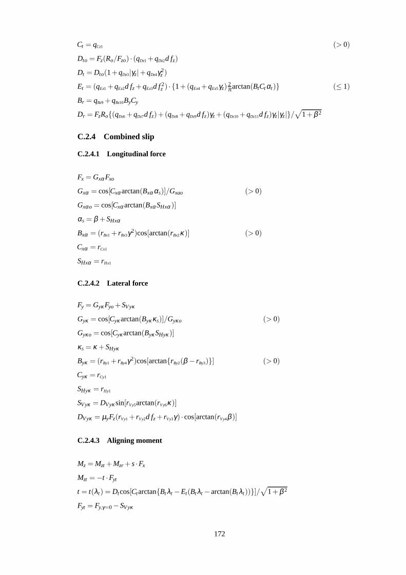
Ct = qCz1 (> 0)
Dto = Fz(Ro/Fzo) · (qDz1 +qDz2d fz)
Dt = Dto(1+qDz3|γz|+qDz4γ2z )
Et = (qEz1 +qEz2d fz +qEz3d f 2z ) · {1+(qEz4 +qEz5γz)
2π arctan(BtCt αt)} (≤ 1)
Br = qBz9 +qBz10ByCy
Dr = FzRo{(qDz6 +qDz7d fz)+(qDz8 +qDz9d fz)γz +(qDz10 +qDz11d fz)γz|γz|}/√
1+β 2
C.2.4 Combined slip
C.2.4.1 Longitudinal force
Fx = Gxα Fxo
Gxα = cos[Cxα arctan(Bxα αS)]/Gxao (> 0)
Gxαo = cos[Cxα arctan(Bxα SHxα )]
αS = β +SHxα
Bxα = (rBx1 + rBx3γ2)cos[arctan(rBx2κ)] (> 0)
Cxα = rCx1
SHxα = rHx1
C.2.4.2 Lateral force
Fy = Gyκ Fyo +SVyκ
Gyκ = cos[Cyκ arctan(Byκ κS)]/Gyκo (> 0)
Gyκo = cos[Cyκ arctan(Byκ SHyκ )]
κS = κ +SHyκ
Byκ = (rBy1 + rBy4γ2)cos[arctan{rBy2(β − rBy3)}] (> 0)
Cyκ = rCy1
SHyκ = rHy1
SVyκ = DVyκ sin[rV y5arctan(rV y6κ)]
DVyκ = µyFz(rVy1 + rVy2d fz + rVy3γ) · cos[arctan(rV y4β )]
C.2.4.3 Aligning moment
Mz = Mzt +Mzr + s ·Fx
Mzt = −t ·Fyt
t = t(λt) = Dtcos[Ctarctan{Bt λt −Et(Btλt − arctan(Bt λt))}]/√
1+β 2
Fyt = Fy,γ=0 −SVyκ
172
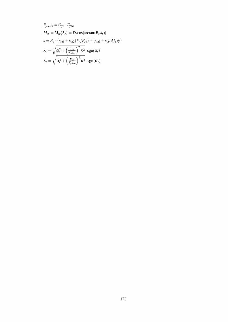
Fy,γ=0 = Gyκ ·Fyoo
Mzr = Mzr(λr) = Drcos[arctan(Brλr)]
s = Ro · {ssz1 + ssz2(Fy/Fzo)+(ssz3 + ssz4d fz)γ}
λt =
√
α2t +
(
KxκKyαoo
)2κ2 · sgn(αt)
λr =
√
α2r +(
KxκKyαoo
)2κ2 · sgn(αr)
173
Bibliography
Abdelkebir, A. (2002). Measurements of inertia, stiffness and damping components of a Suzuki
GSX-R1000. Technical report. Imperial College London, Mechanical Engineering Depart-
ment.
Anon. (1964). Bio-astronautus data book. NASA SP 3006.
Anon. (1993a). BMW statement to all (UK) chief constables.
Anon. (1993b). Boxer comeback. Which Motorcycle pp. 26–32.
Anon. (1993c). An interview with Dr. Goeschel. Motorcycle Sport pp. 234–235.
Anon. (1997a). Chapter 5 of CarsimEd Manual. Mechanical Simulation Corporation. 709 West
Huron, Ann Arbor MI. http://www.carsim.com.
Anon. (1997b). Operating stable. Performance Bikes pp. 44–51.
Anon. (1997c). Safety recall notice, American Suzuki Motor Corporation. Motorcycle.
Anon. (1998). Autosim 2.5+ Reference Manual. Mechanical Simulation Corporation. 709 West
Huron, Ann Arbor MI. http://www.carsim.com.
Bakker, E., H.B. Pacejka and L. Lidner (1989). A new tyre model with an application in vehicle
dynamics studies. SAE 890097.
Bayer, B. (1988). Flattern und pendeln bei kraftradern. Automobil_Industrie 2, 193–197.
Bridges, P. and J.B. Russell (1987). The effect of topboxes on motorcycle stability. Vehicle Sys-
tem Dynamics 16(5–6), 345–354.
Cooper, K.R. (1974). The effects of aerodynamics on the performance and stability of high speed
motorcycles. In: 2nd AIAA Symp. on Aerodynamics of Sport and Competition Automobiles.
Los Angeles.
Cossalter, V. (2002). Motorcycle Dynamics. Race Dynamics. Greendale (WI).
Cossalter, V., A. Doria and R. Lot (1999a). Steady turning of two-wheeled vehicles. Vehicle
System Dynamics 31(3), 157–181.
174
Cossalter, V., A. Doria, R. Lot, N. Ruffo and M. Salvador (2003). Dynamic properties of motor-
cycle and scooter tires: Measurement and comparison. Vehicle System Dynamics 39(5), 329–
352.
Cossalter, V. and R. Lot (2002). A motorcycle multi-body model for real time simulations based
on the natural coordinates approach. Vehicle System Dynamics 37(6), 423–447.
Cossalter, V., M. Da Lio, R. Lot and L. Fabbri (1999b). A general method for the evaluation
of vehicle manoeuvrability with special emphasis on motorcycles. Vehicle System Dynamics
31(2), 113–135.
Cossalter, V., R. Lot and M. Fabiano (2002). The influence of tire properties on the stability of a
motorcycle in straight running and curves. SAE 2002-01-1572.
Cutts, J. (1993). The boxer rebellion. Superbike pp. 4–10.
de Vries, E.J.H. and H.B. Pacejka (1997). Motorcycle tyre measurements and models. In: Proc.
15th IAVSD Symposium on the Dynamics of Vehicles on Roads and on Tracks (L. Palkovics,
Ed.). Budapest Hungary. Suppl. Vehicle System Dynamics, 28, 1998, 280–298.
de Vries, E.J.H and H.B. Pacejka (1998). The effect of tyre modeling on the stability analysis of
a motorcycle. In: Proc. AVEC’98. SAE of Japan. Nagoya. pp. 355–360.
Desoer, C.A. (1969). Slowly varying system x = a(t)x. IEEE Trans Auto Control (Correspon-
dence) AC-14(12), 780–781.
Duke Marketing Ltd (1999). Motorcycle magic.
Duke, O. (1997). Planet bike—Radical thriller or flawed killer. Bike pp. 14–17.
Dunlop (c1977). Wobble and weave videotape.
Eaton, D.J. (1973). Man-Machine dynamics in the stabilization of single-track vehicles. PhD
thesis. University of Michigan.
Evangelou, S. and D.J.N. Limebeer (2000a). Lisp programming of the “sharp 1971” motorcycle
model. http://www.ee.ic.ac.uk/control/motorcycles.
Evangelou, S. and D.J.N. Limebeer (2000b). Lisp programming of the “sharp 1994” motorcycle
model. http://www.ee.ic.ac.uk/control/motorcycles.
Evangelou, S. and D.J.N. Limebeer (2001). Animation of the "sl2001" motorcycle model.
http://www.ee.ic.ac.uk/control/motorcycles.
Evans, J. (1993). BMW R1100RS. Motor Cycle International pp. 58–64.
Farr, K. (1997a). Fats the way to. Motorcycle News.
175
Farr, K. (1997b). Suzuki TL1000 recalled in UK. Motorcycle News.
Farrar, S. (2002). Orritt’s story to explain the phenomena. Times Higher Educational Supple-
ment.
Fujioka, T. and K. Goda (1995a). Discrete brush tire model for calculating tire forces with large
camber angle. In: Proc. 14th IAVSD Symposium on the Dynamics of Vehicles on Roads and
on Tracks (L. Segel, Ed.). Suppl. Vehicle System Dynamics, 25, 1996, 200–216.
Fujioka, T. and K. Goda (1995b). Tire cornering properties at large camber angles: mechanism
of the moment around the vertical axis. JSAE Review 16(3), 257–261.
Giles, C.G. and R.S. Sharp (1983). Static and dynamic stiffness and deflection mode mea-
surements on a motorcycle, with particular reference to steering behaviour. In: Proc. Inst.
Mech. Eng./MIRA Conference on Road Vehicle Handling. Mechanical Engineering Publica-
tions. London. pp. 185–192.
Hales, F.D. (1965). Lateral stability problems of simply articulated vehicles. In: Proceedings of
IUTAM Symposium on Recent Progress in Linear Mechanical Vibrations. pp. 17–34.
Hasegawa, A. (1985). Analysis of controllability and stability of motorcycles – Analysis of
stability at high speed driving. In: 10th International Technical Conference on Experimental
Safety Vehicles. Oxford. pp. 479–500.
Imaizumi, H. and T. Fujioka (1998). Motorcycle-rider system dynamics by multibody dynamics
analysis—effects of the rear load and the suspension assembly on wobble and weave motions.
JSAE Review 19(1), 54–57.
Imaizumi, H., T. Fujioka and M. Omae (1996). Rider model by use of multibody dynamics
analysis. JSAE 17, 75–77.
Ishii, H. and Y. Tezuka (1997). Considerations of turning performance for motorcycles. In: Proc.
SETC’97. Yokohama. pp. 383–389. JSAE 9734601; SAE 972127.
Jennings, G. (1974). A study of motorcycle suspension damping characteristics. SAE 740628.
Kailath, T. (1980). Linear Systems. Chap. 9, p. 607. Prentice-Hall. ISBN 0-13-536961-4.
Kamioka, T., N. Yoshimura and S. Sato (1997). Influence of the front fork on the movement of
a motorcycle. In: Proc. SETC’97. Yokohama. pp. 397–403. SAE 972129.
Kane, T.R. and D.A. Levinson (1983). Multibody dynamics. Transactions of the ASME, Journal
of Applied Mechanics 50, 1071–1078.
Kane, T.R. and D.A. Levinson (1985). Dynamics: theory and applications. McGraw-Hill Series
in Mechanical Engineering. McGraw-Hill. New York.
176
Katayama, T., A. Aoki and T. Nishimi (1988). Control behaviour of motorcycle riders. Vehicle
System Dynamics 17, 211–229.
Knight, M. (2000). Triumph Designs private communication.
Koenen, C. (1983). The dynamic behaviour of motorcycles when running straight ahead and
when cornering. PhD thesis. Delft University of Technology.
Koenen, C. and H.B. Pacejka (1980). Vibrational modes of motorcycles in curves. In: Proc. In-
ternational Motorcycle Safety Conference. Vol. II. Motorcycle Safety Foundation. Washington
DC. pp. 501–543.
Koenen, C. and H.B. Pacejka (1981). The influence of frame elasticity, simple rider body dy-
namics, and tyre moments on free vibrations of motorcycles in curves. In: Proc. 7th IAVSD
Symp. on Dynamics of Veicles on Roads and on Railway Tracks. Swets and Zeitlinger, Lisse.
Cambridge UK. pp. 53–65.
Limebeer, D.J.N., R.S. Sharp and S. Evangelou (2001). The stability of motorcycles under ac-
celeration and braking. Proc. Inst. Mech. Eng. 215(C9), 1095–1109.
Limebeer, D.J.N., R.S. Sharp and S. Evangelou (2002). Motorcycle steering oscillations due to
road profiling. Transactions of the ASME, Journal of Applied Mechanics 69(6), 724–739.
Metropolitan Police (2000). Metropolitan Police, private communication.
Nishimi, T., A. Aoki and T. Katayama (1985). Analysis of straight running stability of motor-
cycles. In: 10th International Technical Conference on Experimental Safety Vehicles. Oxford.
p. 33.
Otto, W.M. (1980). Effect of motorcycle accessories on stability. In: Proc. International Motor-
cycle Safety Conference. Motorcycle Safety Foundation. Linthicum MD 21090, Washington
DC. pp. 1560–1581.
Pacejka, H.B. (2002). Tyre and Vehicle Dynamics. Butterworth Heinemann. Oxford.
Pacejka, H.B. and E. Bakker (1991). The magic formula tyre model. In: Proc. 1st International
Colloquium on Tyre Models for Vehicle Dynamics Analysis. Swets and Zeitlinger, Lisse. Delft.
Suppl. Vehicle System Dynamics, 21, 1993, 1–18.
Pacejka, H.B. and I.J.M. Besselink (1997). Magic formula tyre model with transient proper-
ties. In: Proc. 2nd International Colloquium on Tyre Models for Vehicle Dynamics Analysis.
Berlin. Suppl. Vehicle System Dynamics, 27, 1997, 234–249.
Pacejka, H.B. and R.S. Sharp (1991). Shear force development by pneumatic tyres in steady
state conditions: A review of modelling aspects. Vehicle System Dynamics 20, 121–176.
Raymond, K. (1993). Could do better. Performance Bikes pp. 34–36.
177
Roe, G.E. and T.E. Thorpe (1976). A solution of the low-speed wheel flutter instability in mo-
torcycles. Jour. Mech. Eng. Sci. 18(2), 57–65.
Sakai, H., O. Kanaya and H. Iijima (1979). Effect of main factors on dynamic properties of
motorcycle tires. SAE 790259.
Sayers, M.W. (1991a). Symbolic computer language for multibody systems. Journal of Guid-
ance, Control, and Dynamics 14(6), 1153–1163.
Sayers, M.W. (1991b). Symbolic vector/dyadic multibody formalism for tree-topology systems.
Journal of Guidance, Control, and Dynamics 14(6), 1240–1250.
Segel, L. and R. Wilson (1975). Requirements for describing the mechanics of tires used on
single-track vehicles. In: IAVSD-IUTAM Symp. on Dynamics of Vehicles on Roads and Rail-
way Tracks. Swets and Zeitlinger, Lisse. Delft. pp. 173–186.
Sharp, R.S. (1971). The stability and control of motorcycles. Jour. Mech. Eng. Sci. 13(5), 316–
329.
Sharp, R.S. (1974). The influence of frame flexibility on the lateral stability of motrcycles. Jour.
Mech. Eng. Sci. 15(2), 117–120.
Sharp, R.S. (1976a). The influence of the suspension system on motorcycle weave-mode oscil-
lations. Vehicle System Dynamics 5, 147–154.
Sharp, R.S. (1976b). The stability of motorcycles in acceleration and deceleration. In: Inst.
Mech. Eng. Conference Proceedings on “Braking of Road Vehicles”. MEP. London. pp. 45–
50.
Sharp, R.S. (1985). The lateral dynamics of motorcycles and bicycles. Vehicle System Dynamics
14, 265–283.
Sharp, R.S. (1991). Tyre structural mechanisms influencing shear force generation: Ideas from a
multi-radial-spoke model. In: Proc. 1st International Colloquium on Tyre Models for Vehicle
Dynamics Analysis (H.B. Pacejka, Ed.). Swets and Zeitlinger, Lisse. Delft. Suppl. Vehicle
System Dynamics, 21, 1993, 145–155.
Sharp, R.S. (1994a). The application of multi-body computer codes to road vehicle dynam-
ics modelling problems. Proc. Inst. Mech. Eng., Part D, Journal of Automobile Engineering
208(D1), 55–61.
Sharp, R.S. (1994b). Vibrational modes of motorcycles and their design parameter sensitivities.
In: Vehicle NVH and Refinement, Proc Int Conf.. Mech. Eng. Publications, London. Birming-
ham. pp. 107–121.
178
Sharp, R.S. (2000). Variable geometry active rear suspension for motorcycles. In: Proc. of the
5th International Symposium on Automotive Control (AVEC 2000). Ann Arbor MI. pp. 585–
592.
Sharp, R.S. (2001). Stability, control and steering responses of motorcycles. Vehicle System
Dynamics 35(4–5), 291–318.
Sharp, R.S. and C.J. Alstead (1980). The influence of structural flexibilities on the straight run-
ning stability of motorcycles. Vehicle System Dynamics 9(6), 327–357.
Sharp, R.S. and C.J. Jones (1977). The straight-running stability of single-track vehicles. In:
Proc. 5th IAVSD Symp. on The Dynamics of Vehicles on Roads and on Railway Tracks. Swets
and Zeitlinger, Lisse. Vienna. pp. 334–342.
Sharp, R.S. and D.J.N. Limebeer (2001). A motorcycle model for stability and control analysis.
Multibody System Dynamics 6(2), 123–142.
Sharp, R.S. and M.A. El-Nashar (1986). A generally applicable digital computer based mathe-
matical model for the generation of shear forces by pneumatic tyres. Vehicle System Dynamics
15, 187–209.
Sharp, R.S., D.J.N. Limebeer and M.R. Gani (1999). A motorcycle model for stability and con-
trol analysis. In: Euromech Colloquium 404, Advances in Computational Multibody Dynam-
ics (J.A.C. Ambrosio and W.O. Schiehlen, Eds.). pp. 287–312.
Sharp, R.S., S. Evangelou and D.J.N. Limebeer (2003). Improvements in the modelling of
motorcycle dynamics. In: ECCOMAS Thematic Conference on Advances in Computational
Multibody Dynamics (J.A.C. Ambrósio, Ed.). Lisbon. MB2003-029 (CD-ROM).
Singh, D.V. and V.K. Goel (1975). Stability of single track vehicles. In: IAVSD-IUTAM Symp.
on Dynamics of Vehicles on Roads and Railway Tracks. Swets and Zeitlinger, Lisse. Delft.
pp. 187–196.
Singh, D.V., V.K. Goel and M. Bhattacharya (1974). Rolling characteristics of small size pneu-
matic tyres. Proc. Inst. Mech. Engrs. 188(AD), 701–713.
Skoog, R.A. and C.G.Y. Lau (1972). Instability of slowly varying systems. IEEE Trans Auto
Control AC-17(1), 86–92.
Spierings, P.T.J. (1981). The effects of lateral front fork flexibility on the vibrational modes of
straight-running single-track vehicles. Vehicle System Dynamics 10(1), 21–35.
Steele, Jr. and L. Guy (1984). COMMON LISP: the language. Digital Press. Burlington, Mass.
Strang, G. (1988). Linear Algebra and its applications. 3rd ed.. Saunders HBJ.
179
Takahashi, T., T. Tatsuo and T. Nakamura (1984). Experimental and theoretical study of the
influence of tires on straight-running motorcycle weave response. SAE 840248.
Tezuka, Y., H. Ishii and S. Kiyota (2001). Application of the magic formula tire model to mo-
torcycle maneuverability analysis. JSAE Review 22, 305–310.
The Mathworks Inc. (2000). MATLAB 6 Reference Manual. http://www.mathworks.com.
van Oosten, J.J.M., E. Kuiper, G. Leister, D. Bode, H. Schindler, J. Tischleder and S. Köhne
(2003). A new tyre model for TIME measurement data. in press.
Weir, D.H. (1972). Motorcycle handling dynamics and rider control and the effect of design con-
figuration on response and performance. PhD thesis. University of California at Los Angeles.
Weir, D.H. and J.W. Zellner (1978). Lateral-directional motorcycle dynamics and rider control.
SAE 780304.
Weir, D.H. and J.W. Zellner (1979). Experimental investigation of the transient behaviour of
motorcycles. SAE 790266.
Zellner, J.W. and D.H. Weir (1978). Development of handling test procedures for motorcycles.
SAE 780313.
180