DYNAMIC STABILITY OF SPACE VEHICLES

NASA CONTRACTOR

REPORT

DYNAMIC STABILITY

NASA

:. % V.11 c.1

OF SPACE VEHICLES

Volume XI - Entry Disturbance

and Control

by F. D. Steketee

Prepared by

GENERAL DYNAMICS CORPORATION

: ‘:.

San Diego, Calif.

for George C. Marshall Space Flight Center

NATIONAL AERONAUTICS AND SPACE ADMINISTRATION . WASHINGTON, D. C. . NOVEMBER 1967

TECH LIBRARY KAFB, NM

00b0030 NASA CR- 945

DYNAMIC STABILITY OF SPACE VEHICLES

Volume XI - Entry Disturbance and Control

By F. D. Steketee

Distribution of this report is provided in the interest of information exchange. Responsibility for the contents resides in the author or organization that prepared it.

Issued by Originator as Report No. GDC-BTD67-023

Prepared under Contract No. NAS 8-11486 by GENERAL DYNAMICS CORPORATION

San Diego, Calif.

for George C. Marshall Space Flight Center

NATIONAL AERONAUTICS AND SPACE ADMINISTRATION

For sole by the Clearinghouse for Federal Scientific and Technical Information Springfield, Virginia 22151 - CFSTI price $3.00

FOREWORD

This report is one of a series in the field of structural dynamics prepared under contract NAS 8-11486. The series of reports is intended to illustrate methods used to determine parameters required for the design and analysis of flight control systems of space vehicles. Below is a complete list of the reports of the series.

Volume I Volume II Volume III Volume IV Volume V Volume VI Volume VII

Volume VIII

Volume IX

Volume X Volume XI Volume XII Volume XIII

Volume XIV Volume XV

Lateral Vibration Modes Determination of Longitudinal Vibration Modes Torsional Vibration Modes Full Scale Testing for Flight Control Parameters Impedence Testing for Flight Control Parameters Full Scale Dynamic Testing for Mode Determination The Dynamics of Liquids in Fixed and Moving

Containers Atmospheric Disturbances that Affect Flight Control

Analysis The Effect of Liftoff Dynamics on Launch Vehicle

Stability and Control Exit Stability Entry Disturbance and Control Re-entry Vehicle Landing Ability and Control Aerodynamic Model Tests for Control Parameters

Determination Testing for Booster Propellant Sloshing Parameters Shell Dynamics with Special Applications to

Control Problems

The work was conducted under the direction of Clyde D. Baker and George F. McDonough, Aero Astro Dynamics Laboratory, George C. Marshall Space Flight Center. The General Dynamics Convair Program was conducted under the direction of David R. Lukens.

. . . 111

TABLE OF CONTENTS

Section Page

1 INTRODUCTION . . . . . . , . . . . . . . . . 1

2 STATEOFTHEART . . . . . . . , . . . . . . . 5

3 DESIGN CRITERIA. . . . . . . . . .

3.1 Re-entry Corridor . . , . . . . 3.2 Handling Criteria. . . . . . . .

3.2.1 Desired Control System Characteristics 3.2.2 Longitudinal Stability and Control . . 3.2.3 Lateral/Directional Stability . . . .

3.3 Disturbances . . . . . . . . .

3.3.1 Upper Atmospheric Density . . . .

4 CONTROLMETHODS. . . . . . . . . . . . . . .

. . . . . .

......

......

......

......

......

. . . . . .

4.1 Constant L/D Vehicles 1 : 1 1 . . .

4.1.1 Relationship Between Control and Guidance 4.1.2 Typical Control System . . . . . . .

4.2 Variable L/D Vehicles . . . . . . .

. . . . .

. . . . .

. . . . .

4.2.1 Relationship Between Control and Guidance 4.2.2 Typical Control System. . . . . . . 4.2.3 Possible Problem Areas . . . . . .

. . . . .

. . . . .

4.3 Experimental Control Techniques . . .

4.3.1 Movable Nose Spike . . . . . . . . . . . . . 4.3.2 Magnetohydrodynamic Flight Control . . . . . . . 4.3.3 Variable-Drag Devices . . . . . . . . . . . . 4.3.4 Augmented Minimum Systems. . . . . . . . . .

4.4 Unmanned Re-entry Vehicles . . . . . . . . . .

5 ANALYSIS ..................

5.1 Small Perturbation Equations. .........

5.1.1 Euler Angles ............... 5.1.2 Expansion of the Gravity Force ......... 5.1.3 Equations of Elastic Vibrations .........

7

7 9

9 10 13

15

15

19

19

19 21

22

22 24 26

29

29 29 30 30

31

33

33

36 37 40

V

Section

6

TABLE OF CONTENTS, Contd

Page

5.2 Variable Density Solution ........... 44

5.2.1 Equations of Motion ............. 44 5.2.2 Bessel Function Solution ........... 47 5.2.3 Solutions for Special Cases .......... 50

REFERENCES . . . . . . . . . . . . . , . . . 53

vi

LIST OF ILLUSTRATIONS

c 1

2

3

4

5

6

7

8

9

10

11

12

13

14

15

16

17

Control System Design Interconnection Diagram . . .

Re-entry Operational Constraints 1. . . . . . . .

12-G Corridor Depth . . . . . . . . . . . .

Longitudinal Short Period Dynamics Requirements for Normal Operation . . . . . . . . . . . . .

Longitudinal Short Period Dynamics Requirements for Emergency Operation . . . . . . . . . . . .

Measured Variations in Air,Density versus 1959 ARDC Standard Atmosphere (Ref. 34) . . . . . . . . .

Typical Landing Capability from Circular Orbit. . . .

Approximate Weight Penalty versus L/D Ratio . . . .

One-man M2-F2 Inboard Profile. . . . . . . . .

Four-man HL-10 Inboard Profile . . . . . . . .

Typical L/D and CL Data versus Angle of Attack . . .

Vehicle Coordinate System . . . . . . . . . .

Acceleration Components . . . . . . . . . . .

Gravity Force in the Steady-State Condition, Pitch Plane

Elastic Vehicle in the Pitch Plane . . . . . . . .

Elastic Vehicle in Yaw Plane . . . . . . . . .

Vehicle Flight Parameters. . . . . . . . . . .

. . .

. . .

. . .

. . .

. . .

. . . 17

. . . 20

. . . 20

. . . 23

. . . 23

. . . 25

. . . 34

. . . 38

. . . 38

. . . 42

. . . 43

. . . 45

2

7

8

11

12

vii

.NOMENCLATURE

a = acceleration vector

A = reference area

b = reference length

(‘A 9 ‘y 9 CN) = axial, side, and normal force coefficients

q, s cm 9 Cn) = roll, pitch, and yaw moment coefficients

cL = lift coefficient

D = drag

F = force vector

F i

= force vector acting on element of mass, mi

(TFx, CFy, CFZ) = total perturbation force acting parallel to vehicle body axes

[ fp (a , t), fy (4 , t), fr (a , t)] = force (moment) causing bending (torsion) in pitch, yaw, and roll planes.

g = gravity acceleration

gl = U,” apparent acceleration due to gravity, g - r

GO = moment of external forces about origin of inertial coordinates

GS, = moment of external forces about origin of body axis system

HO = angular momentum

HS, = angular momentum

CHx 9 Hy P Hz) = components of i$, in body axis system

‘In 3 Iyy s Iz,) = moment of inertia of reduced vehicle about vehicle body axes _

I = unit matrix

I r

(a) = moment of inertia per unit length of reduc.ed vehicle about longitudinal axis of vehicle

‘Ixy 9 Ixz 9 Iyz) = product of inertia of reduced vehicle about vehicle body sxes

ix

i, i, k = unit vector triad in body axis system

Ji (6) = Bessel function of the first kind and order i

K1 = a constant defined by Equation 45

K2 = a constant defined by Equation 47

a = length parameter along vehicle longitudinal axis; positive in aft direction

AQ = distance from center of pressure in pitch plane to origin of body axis system

a B

= distance from center of pressure in yaw plane to origin of body axis system

L/D = lift-to-drag ratio

L’ = [Li +(Ixz/In)Ni) l/cl- (I~s/I~ zz I i

) J = principal axis roll acceleration

due to external torques (i)

L P

= PsUob2C JP

/41*

Lr = PsUob2Clp/41n

LP = qAbC&

La = qAbCQb/Ixx

m. = element of mass 1 L

m(1) = reduced mass per unit length along vehicle longitudinal axis: Jf

m(a) dA = m. 0

m 0

= reduced mass of vehicle ( = Mt - cm .) i Pl

Mc = total mass of vehicle

i (MO

P , M@, Mf)) =

Y

GM,, cMy, CMZ ) =

Ni’ = ‘Nif(lxz’lzz)

generalized mass of i th

bending mode in (pitch, yaw, roll) plane

total perturbation moment along vehicle body axes

Li I/ r 1 - (IZz / I I xx zz

) I = principal axis yaw acceleration

due to external torques (i)

N P

= pAUob2 Cnp/41 zz

X

Nr = PAUob2 Cnr/41zz

NV = Ns/Uo

Ns = q A b Cnb / Izz

Nb = qAbCn6/I zz

(P , Q , R) = angular velocities defined by Figure 12

PO 9 Q. 9 R. ) = steady-state values of P, Q, and R

(p , q , r) = perturbation values of P, Q, and R

(<) , qr , qf) ) = generalized coordinate of ith bending mode in pitch, yaw, and roll planes

i (Q( ) , Qli) (i) .th

P Y , Qr ) = generalized force (moment) of I bending mode in pitch, yaw,

and roll planes

8 = Laplace operator

t = time

TS = spiral mode time constant

T = roll mode time constant r

(U, V, W) = components of velocity vector of origin of body axis system

w. 3 v. 9 W. ) = steady-state values of U, V, and W

<uw 9 VW 9 W, ) = components of wind velocity vector in body axis system

(u, v, w) = perturbation values of U, V, and W

ve = horizontal velocity component

vE = atmospheric entrance velocity

(x, y, z) = coordinates specifying location of element of mass in body axis system

(x IY cg cg 9 zcg) = coordinates specifying location of c. g. of reduced vehicle relative

to body axis system

Yi (5) = Bessel function of the second kind and order i

Y6=qAC /m Yb 0

xi

Cy = perturbation angle of attack in pitch plane

o! 9

= nominal angle of attack

CY t

= total angle of attack

@ = perturbation angle of attack in yaw plane

y = perturbation flight-path angle ( = o! - 8)

yE = atmospheric entrance flight path

yS = nominal flight-path angle

Yt = total flight-path angle

< d

= dutch roll damping coefficient

p #

= lateral mode numerator “damping” coefficient

(c (9 P

,. c y 0) , cf) ) = relative damping ratio for ith bending mode in pitch, yaw, and roll planes

(6, $ , ‘p) = perturbation attitude angle in pitch, yaw, and roll planes

8 = nominal Pitch attitude

et = total pitch attitude

x = radius vector from origin of inertial reference to origin of body axis system

/J = velocity vector from origin of inertial reference to origin of body axis system

7 = constant in density-altitude relation

= (22,000 ft)-l

5 = earth’s rotational rate

[ 5, (a, t), ey (a, t), 4, (A, t) 1 = bending (torsion) deflection in pitch, yaw, and roll planes

p = atmospheric density

6 = radius vector from element of mass to origin of body axis system

P C

= radius vector from c. g. of reduced mass of vehicle to origin of body axis system

0 = density ratio p / p.

xii

@ , aW , o (9 - r ) - negative slope of ifh bending mode in pitch, yaw, and roll planes; P Y

( -&p() i i -a& i +o()

= g-s-$-- alir >

p (9 , cp (9 , ’ 9:’ ) = normalized mode shape fundicm for the i th

bending (@r&on) mode P Y

Wd = dutch roll frequency

% = lateral mode numerator frequency

p (i) , o 0) , o 0) th _ P Y

r ) - undamped natural frequency of the i bending mode in lhe pitch, yaw, and roll planes

3 = velocity vector of body axis coordinate frame relative to earth axie

(7 = a vector

(‘) = derivative with respect to time in local coordinate frame

( 10 = steady-state value

xiii

l/INTRODUCTION

This monograph is intended to serve as a gui& for the design of re-entry vehicle control systems, from a systems standpoint. In some cases the depth of a particular field prevents a detailed treatment; however, the reference section has been compiled to represent the latest recognized work in the various disciplines. It should be pointed out that the field of re-entry control is advancing rapidly in several areas; the serious investigator should be careful, therefore, that his material represents the latest en- deavors.

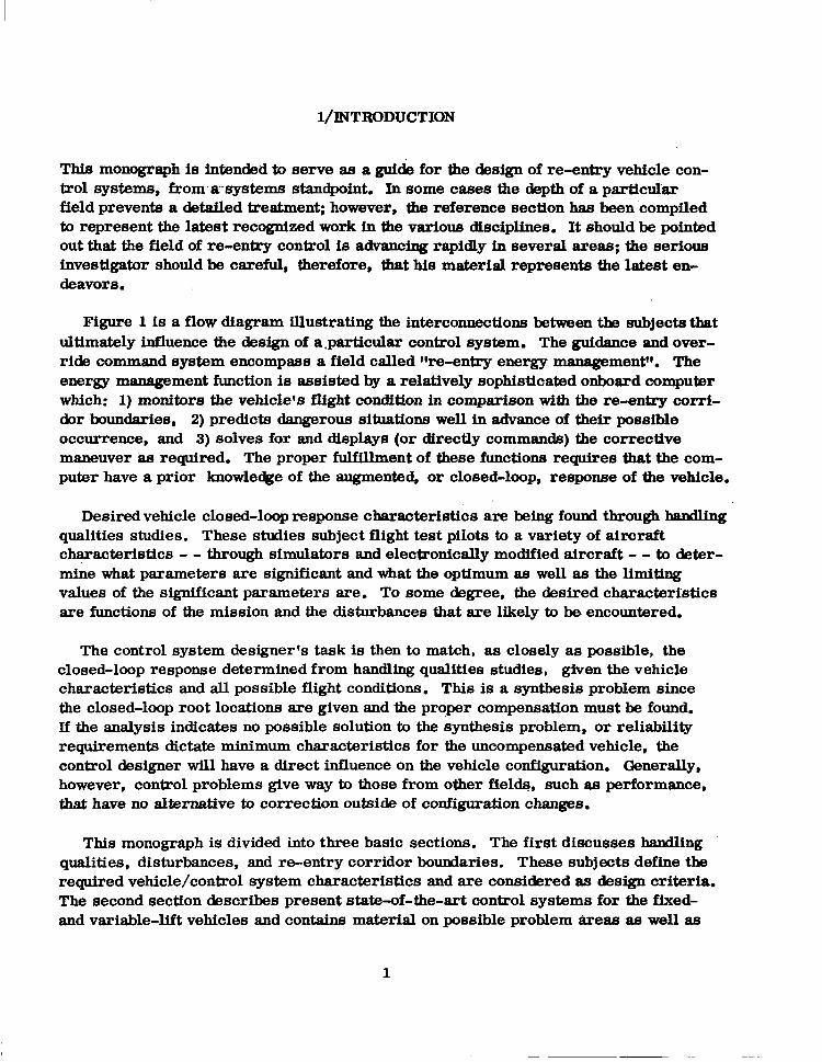
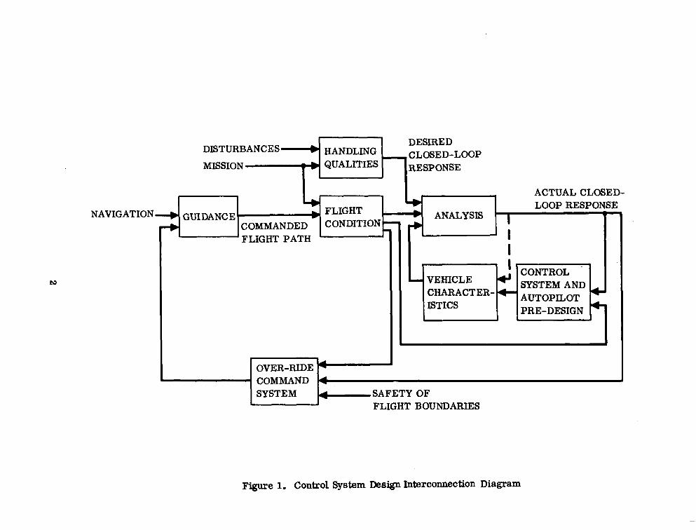
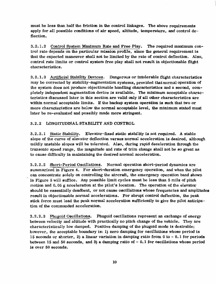
Figure 1 is a flow diagram illustrating the interconnections between the subjectsthat ultimately influence the design of a.particular control system. The guidance and override command system encompass a field cslled fVe-entry energy management”. The energy management function is assisted by a relatively sophisticated onboard computer which: 1) monitors the vehicle’s flight condition in comparison with the re-enlry cod- dor boundaries, 2) predicts dangerous situations well in advance of their possible occurrence, and 3) solves for and displays (or directly commands) the corrective maneuver ‘as required. The proper fuIfillment of these functions requires that the computer have a prior lmowleae of the augmented, or closed-loop, response of the vehicle.

Desired vehicle closed-loop response characteristics are being fouxxi through handling qualities studies. These studies subject flight test pilots to a variety of aircraft characteristics - - through simulators and electronically modified aircraft - - to determine what parameters are significant and what the optimum as well as the limiting values of the significant parameters are. To some degree, the desired characteristics are functions of the mission and the disturbances that are likely to be encountered.

The control system designer’s task is then to match, as closely as possible, the closed-loop response determined from handling qualities studies, given the vehicle characteristics and all possible flight conditions. This is a synthesis problem since the closed-loop root locations are given and the proper compensation must be found. If the analysis indicates no possible solution to the synthesis problem, or reliability requirements dictate minimum characteristics for the uncompensated vehicle, the control designer will have a direct influence on the vehicle configuration. Generally, however, control problems give way to those from other fields, such as performance, that have no alternative to correction outside of configuration changes.

This monograph is divided into three basic sections. The first diecusses handling qualities, disturbances, and re-entry corridor boundaries. These subjects define the required vehicle/control system characteristics and are considered as design criteria. The second section &scribes present state-of-the-art control systems for the fixed- and variable-lift vehicles and contains material on possible problem irreas as well as

1

tu

DESIRED CLOSED-LOOP RESPONSE

ACTUAL CLOSED-

NAVIGATION + GUI DANC E + FLIGHT .-

LOOP RESPONSE l ANALYSIS ’ fi I

I 1

-FLIGHT PATH -

. I’ I- 3

COMMAND SYSTEM d-SAFETY OF

FLIGHT BOUNDARIES

[ OVER-RIDE r-

Figure 1. Control System Design Interconnection Diagram

a discussion of some new experimental control techniques. The purpose of this second section is to illustrate how re-entry control systems are currently being designed and to point out some of the problem areas that the &signer should be aware of. The third section develops the small perturbation equations that are required for the analysis/ synthesis problem. This section also expands the pitch mode equation to include density as an exponential function of altitude.

3

B/STATE OF THE ART

The field of re-entry control can be considered as consisting of three subjects: configuration studies, stability analyses, and handling criteria investigations. The configuration studies can be subdivided into 1) the constant, and relatively low, L/D (lift/ drag) vehicles typified by the Mercury-Gemini-Apollo series, and 2) the variable-lift vehicles. The state of the art in the constant L/D vehicles is represented, of course, by Apollo. The majority of present-day research is involved with the variable L/D vehicles because of their advantages of wide range and conventional landing capability. NASA is doing the, bulk of the configuration investigations of variable L/D shapes. These investigations, which are primarily wind tunnel studies, have been strongly influenced by past experience with the X-15 and by what is presently known regarding necessary handling characteristics. To date this evolutionary process has produced the HL-10, a vehicle that can be considered as representing the state of the art in re- entry control.

Cornell Aeronautical Laboratory is the leader, although not the sole contributor, in the field of defining handling requirements. In addition to fixed and moving base simulator& considerable work is being done with Wariable st.abilitytV aircraft. These aircraft have their short-period dynamics modified by a special form of autopilot to represent a selected re-entry vehicle. In addition, variable-drag devices are installed to approximate the L/D ratio of the re-entry configuration. The wide interest in handling requirements for re-entry vehicles stems from the fact that the flight regime is well beyond the areas used to define conventional aircraft handling requirements; and the rather unusual shapes imply that the handling quality boundaries should be clearly defined since unneeded modifications for handling tend to be costly in terms of performance.

Stability analysis generally follows the well known small perturbation techniques that have been successfully applied to the design of aircraft and missile autopilots in the past. A slight modification is the inclusion of the centripetal force term due to the very high velocity of the vehicle. Techniques have been developed for including terms due to the change in atmospheric density. Including these terms results in time-variable- parameter systems that can, in some cases, be solved by the frequency-transformation approach, or the second method of Liapunov, or other sophisticated techniques. How- ever, the difficulty in applying these techniques to a particular engineering problem has prevented their wide usage.

5

3/DESIGN CRITlZ RIA

3.1 RE-ENTRY CORRIDOR

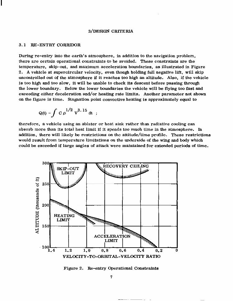
During re-entry into the earth’s atmosphere, in addition to the navigation problem, there are certain operational constraints,to be avoided. These constraints are the temperature, skip-out, and maximum acceleration boundaries, as illustrated in Figure 2. A vehicle at supercircular velocity, even though holding full negative lift, will skip uncontrolled out of the atmosphere if it reaches too high an altitude. Also, if the vehicle is too high and too slow, it will be unable to check its descent before passing through the lower boundary. Below the lower boundaries the vehicle will be flying too fast and exceeding either deceleration and/or heating rate limits. Another parameter not shown on the figure is time. Stagnation point convective heating is approximately equal to

Q(t) = f C 01’2 V3. l5 dt ;

therefore, a vehicle using an ablater or heat sink rather than radiative cooling can absorb more than its total heat limit if it spends too much time in the atmosphere. In addition, there will likely be restrictions on the attitude/time profile. These restrictions would result from temperature limitations on the underside of the wing and body which could be exceeded if large angles of atta&were maintained for extended periods of time.

% SKIP-OUT

4 1.2 1.0 0.8 0.6 6.4 0.2 VELOCITY-TO-ORBITAL-VELOCITY RATIO

.Y CEILING

Figure 2. Re-entry Operational Constraints

7

100

YO

60

2 ‘0 E . = 60

2 g 50

i 40

d o 30

20

10

0 30 40 50 60 10 80 00 loo

The width of the re-entry corridor, as might be expected, is closely related to the penetration velocity. It is ah30 a function of tlm3 allowable acceleration and maximum hypersonic lift-to-drag ratio of the vehicle. Figure 3 illustrates the variation of entry corridor width versus velocity for several L/D ratios and a deceleration limit of 12 g. Note the increased tolerance in entry corridor width for the variable (modulated) lift vehicles.

EARTH ENTRY VELOCITY (thouunda of It/m)

Figure 3. 12-G Corridor Depth

Supercircular re-entry undoubtedly poses the more etringent requirements on the control system, since the skip-out boundary must be avoided. Skip-out is prevented by a carefully timed and executed maneuver to a maximum negative lift attitude. This maneuver must be accomplished shortly after the pull out (e. g. , when Y = 0) and at a relatively low altitude, or the flight-path angle will rapidly increase due to the initially high dynamic pressure. If the maneuver is accomplished too late, the rate of climb and vertical momentum will build up to values which cannot then be easily overcome in the low density of the higher altitude. Conversely, over-control of the maneuver would result in a dangerous rapid dive-in trajectory.

There are two possible methods of reversing the lift vector: roll the vehicle 180 degrees or pitch the vehicle down to a negative attitude. If the latter maneuver is chosen, the vehicle must be rotated through 40 to 50 degrees. to a negative angle of attack of approximately -45 degrees. The obvious implications are that the vehicle must be trimmable and controllable in this unusual attitude. A possible troublesome controllability characteristic would be the likely negative dihedral effect that would result from the negative angle of attack. The roll maneuver would appear to be a far better choice; however, vehicle roll characterietice must be such as to permit this precise and relatively rapid maneuver to occur near the peak load factor. For a vehicle with a roll rate capability of 20 deg/sec entering the atmosphere at a velocity of 36,000 ft/sec, there ie a lo-second interval during which the roll can be initiated without the vehicle’s skipping back out of the atmosphere or exceeding sn deceleration loading of 10 g. For an entry speed of 70,000 ft/eec the time interval is about one second.

8

During re-entry, control of the vehicle must be transferred from a purely reaction control system to an aerodynamic system for the variable-lift vehicles. This change- over must be smooth and require no unusual piloting techniques.

Generally, the flight condition/vehicle situation will produce a longitudinal short- period mode whose frequency is too low for normal operation. This appears to be true for altitudes down to at least 100,000 feet, by which time the re-entry maneuver is essentially complete. The implication is that a stability-augmentation device that raises the vehicle’s natural frequency as well as the damping will usually be required.

3.2 HANDLING CRlTERIA

Generally, re-entry vehicles will be under the more or lerr direct control of a human pilot. Automatic control is possible, but even in this case the vehicle-control ayatem, or inner loop, must be reaeonably well behaved so that the guidance, or outer loop, will adequately perform ite,,task, To a large extent, handling quality rpecificatlonr are based on mieeion requirements. For Instance, fighter-type aircraft must have much higher roll rates and roll acceleration8 than bombers. Similarly, the roll rate and roll acceleration characterietics of a variable-lift vehicle returning from Mars are more crit- ical than a constant L/D vehicle returning from orbit, since the former must perform a precisely timed and executed roll maneuver in order to prevent atmospheric skip-out. The factors that influence controllability (which is a fundamental requirement pertinent to re-entry vehicles as well as to more conventional aircraft) are reasonably well known; however, refinements and additions are continuously being considered. At the present time several major handling quality requirements studies are in progress. In particular, Cornell Laboratory has studies underway using a variable-stability T-33 aircraft and fixed-base simulators which are slanted toward re-entry vehicles. The basic document delineating handling requirements for aircraft is Military Specification MIL-F-8785 (ASG), Reference 9. Reference 1, the Cornell Aeronautical Laboratory report on hyper- velocity aircraft handling quality requirements, is a refinement and improvement on MIL-F-8785 since it is particularly slanted toward re-entry vehicles. These two documents provide a good foundation for the handling quality specifications of a re-entry vehicle.

The handling quality requirements listed in References 1 and 9 are quite detailed and no attempt will be made to completely cover them here, Rather, the aspects pertinent to re-entry will be discussed, and additional work as reported in References 2 through 8 will be included where applicable.

3.2.1 DESIRED CONTROL SYSTEM CHARACTERISTICS

3.2.1.1 Friction and Breakout Force. About all axes, and for all normal trim settings, the controls shall exhibit positive centering. The centering accuracy should be sufficient to prevent large departures from trim, or any other objectional flight characteristics, with controls free. For hydraulic control systems, friction within the hydraulic valve

9

must be less than half the friction in the control linkages. The above requirements apply for all possible conditions of air speed, altitude, temperature, and control deflection.

3.2.1.2 Control System Maximum Rate an.d Free Play. The required maximum control rate depends on the particular mission profile, since the general requirement is that the expected maneuver shall not be limited by the rate of control deflection. Also, control rate limits or control system free play shall not result in objectionable flight characteristics.

3.2.1.3 Artificial Stability Devices. Dangerous or intolerable flight characteristics may be corrected by stability-augmentation systems, provided that normal operation of the system does not produce objectionable handling characteristics and a second, completely independent augmentation device is available. The minimum acceptable characteristics discussed later in this section are valid only if all other characteristics are within normal acceptable limits. If the backup system operation is such that two or more characteristics are below the normal acceptable level, the minimum stated must later be re.-evaluated and possibly made more stringent.

3.2.2 LONGITUDINAL STABILITY AND CONTROL

3.2.2.1 Static Stability. Elevator-fixed static stability is not required. A stable slope of the curve of elevator deflection versus normal acceleration is desired, although mildly unstable slopes will be tolerated. Also, during rapid deceleration through the trsnsonic speed range, the magnitude and rate of trim change shall not be so great as to cause difficulty in maintaining the desired normal acceleration.

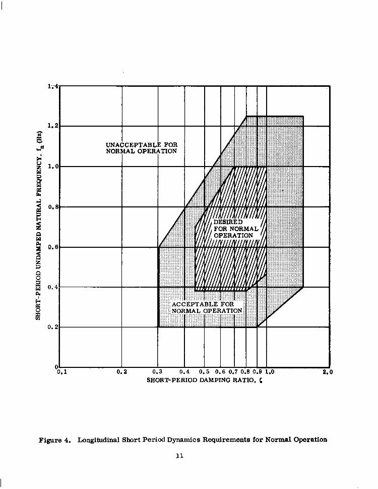
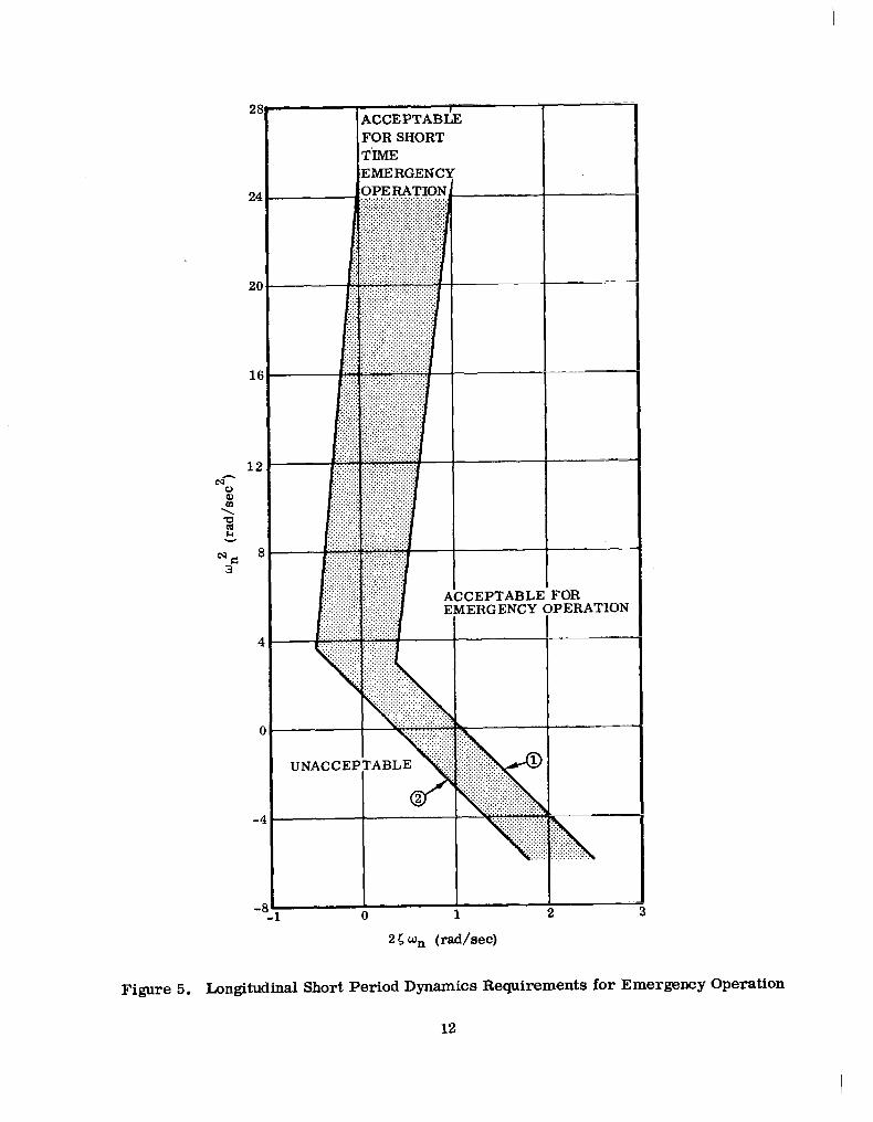
3.2.2.2 Short-Period Oscillations. Normal operation short-period dynamics are summarized in Figure 4. For short-duration emergency operation, and when the pilot can concentrate solely on controlling the aircraft, the emergency operation band shown in Figure 5 will suffice. Any possible limit cycles must be less than 5 mils of pitch motion and 0.05 g acceleration at the pilot’s location. The operation of the elevator should be essentially deadbeat, or not cause oscillations whose frequencies and amplitudes result in objectionable normal accelerations. For abrupt control deflection, the peak stick force must lead the peak normal acceleration sufficiently to give the pilot anticipa- tion of the commanded acceleration.

3.2.2.3 Phugoid Oscillations. Phugoid oscillations represent an exchange of energy between velocity and altitude with practically no pitch change of the vehicle. They are characteristically low damped. Positive damping of the phugoid mode is desirable; however, the acceptable boundary is: 1) zero damping for oscillations whose period is 15 seconds or shorter, 2) a linear variation in damping ratio from 0 to - 0.1 for periods between 15 and 50 seconds, and 3) a damping ratio of - 0.1 for oscillations whose period is over 50 seconds.

10

1.2

-I - I P P UNACCEPTABI UNACCEPTABI

NORMAL OPEIi NORMAL OPEIi . . e e 2 2 1.0 1.0 g g 8 8 E E d d i i 0.6 0.6

52 52

! ! f f 0.6 0.6

g g

s s 2 2 7 7 0.4 0.4

0.2 0.2

O- 0.1 0.2 C “0.1 0.2 C 0.4 0.5 0.6 0.7 0.6 0.B 1.0 2 SHORT-PERIOD DAMPING RATIO, C

Figure 4. Longitudinal Short Period Dynamics Requirements for Normal Operation

11

ACCEPTABLk FOR SHORT T’iMJZ EMERGENCY

0 1 2 2 6 w, (rad/eec)

Figure 5. Longitudinal Short Period Dynamics Requirements for Emergency Operation

12

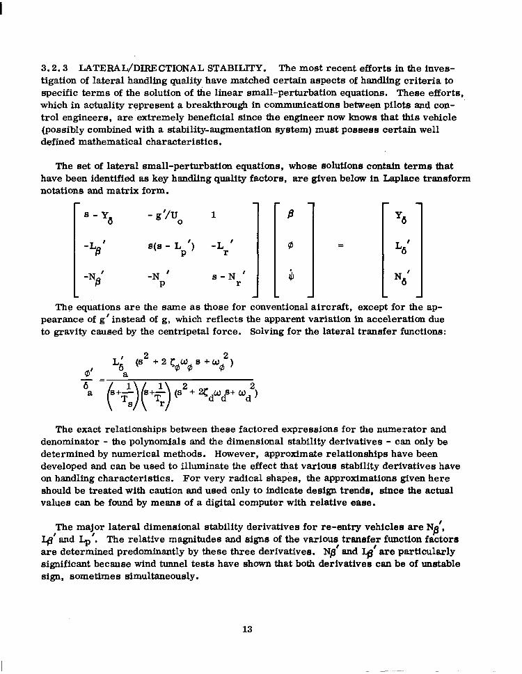
3.2.3 LATERAL/DIRECTIONAL STABILITY. The most recent efforts in the investigation of lateral handling quality have matched certain aspects of handling criteria to specific terms of the solution of the linear small-perturbation equations. These efforts, which in actuality represent a breakthrough in communications between pilots and control engineers, are extremely beneficial since the engineer now knows that this vehicle (possibly combined with a stability-augmentation system) must possess certain well defined mathematical characteristics.

The set of lateral small-perturbation equations, whose Bolutions contain terms that have been identified as key handling quality factors, are given below in Laplace transform notations and matrix form.

B-Y 6 - g’/u 1 0

B(S - Lp’) -Lr’

-N ’ P

B-N I

r

=

. m

y&

La’

N6’

The equations are the same as those for conventional aircraft, except for the appearance of g’ instead of g, which reflects the apparent variation in acceleration due to gravity caused by the centripetal force. Solving for the lateral transfer functions:

’ (B2 +2 57 +Wg2)

a

i;)( ) 1 Bf-

TS

s+$- (B2 + 2rdwds+ W,2) r

The exact relationships between these factored expressions for the numerator and denominator - the polynomials and the dimensional stability derivatives - can only be determined by numerical methods. However, approximate relationships have been developed and can be used to illuminate the effect that various stability derivatives have on handling characteristics. For very radical shapes, the approximations given here should be treated with caution and used only to indicate design trends, since the actual values can be found by means of a digital computer with relative ease.

The major lateral dimensional stability derivatives for re-entry vehicles are Np’, L,g’and II,‘. The relative magnitudes and signs of the various tranefer function factors are determined predominantly by these three derivatives. N@’ and 9’ are particularly significant because wind tunnel tests have shown that both derivatives can be of unstable sign, sometimes simultaneously.

13

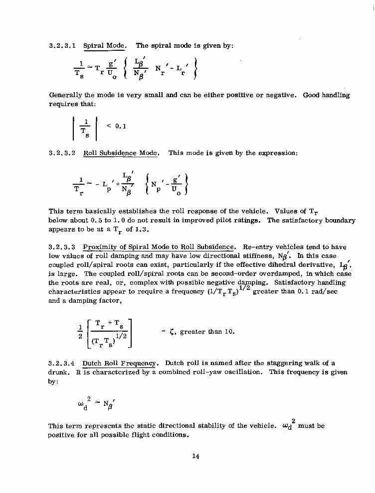
3.2.3.1 Spiral Mode. The spiral mode is given by:

‘Generally the mode is very small and can be either positive or negative. Good handling requires that:

1

T < 0.1

3.2.3.2 Roll Subsidence Mode. This mode is given by the expression:

This term basically establishes the roll response of the vehicle. Values of Tr below about 0.5 to 1.0 do not result in improved pilot ratings. The satisfactory boundary appears to be at a T, of 1.3.

3.2.3.3 Proximity of Spiral Mode to Roll Subsidence. Re-entry vehicles tend to have low values of roll damping and may have low directional stiffness, Np’. In this case coupled roll/spiral roots can exist, particularly if the effective dihedral derivative, 49’1 is large. The coupled roll/spiral roots can be second-order overdamped, in which case the roots are real, or, complex with possible negative da ping. Satisfactory handling characteristics appear to require a frequency (l/T, T,) 1E greater than 0.1 rad/sec and a damping factor,

1 Tr + TS z [ 1 l/2 = c, greater than 10.

(T&l

3.2.3.4 Dutch Roll Frequency. Dutch roll is named after the staggering walk of a drunk. It is characterized by a combined roll-yaw oscillation. This frequency is given by:

This term represents the static directional stability of the vehicle. Ud2 must be positive for all possible flight conditions.

14

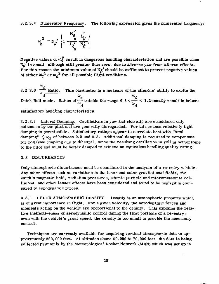
3.2.3.5 Numerator Frequency. The following expression gives the numerator frequency:

Negative values of WJ result in dangerous handling characteristics and are possible when N@’ is small, although still greater thsn zero, due to adverse yaw from aileron effects. For this reason the minimum value of Np’ should be sufficient to prevent negative values of either WC or Wd2 for all possible flight conditions.

3.2.3.6 3 o Ratio. This parameter is a measure of the ailerons’ ability to excite the d

Dutch Roll mode. % % RatlOB of - outside the range 0.8 < w < 1.2 usually result in below-

Wd d satisfactory handling characteristics.

3.2.3.7 Lateral Damping. Oscillations in yaw and side slip are considered only nuisances by the pilot and are generally disregarded. For this reason relatively light damping is permissible. Satisfactory ratings appear to correlate best with “total damping” l;dq of between 0.2 and 0.3. Additional damping is required to compensate for roll/yaw coupling due to dihedral, since the resulting oscillation in roll is bothersome to the pilot and must be better damped to achieve an equivalent handling quality rating.

3.3 DISTURBANCES

Only atmospheric disturbances need be considered in the analysis of a re-entry vehicle. Any other effects such as variations in the lunar and solar gravitational fields, the earth’s magnetic field, radiation pressures, atomic particle and micrometeorite col- lisions, and other lesser effects have been considered and found to be negligible compared to aerodynamic forces.

3.3.1 UPPER ATMOSPHERIC DENSITY. Density is an atmospheric property which is of great importance in flight. For a given velocity, the aerodynamic forces and moments acting on the vehicle are proportional to the density. This explains the relative ineffectiveness of aerodynamic control during the first portions of a re-entry; even with the VehiCk'B great speed, the density is too small to provide the necessary control.

Techniques are currently available for acquiring vertical atmospheric data to approximately 220,000 feet. At altitudes above 60,000 to 70,000 feet, the data is being collected primarily by the Meteorological Rocket Network (MRN) which was set up in

15

October 1959. Data from this source gives detailed information on the upper atmosphere. for the vicinity of the North American continent only.

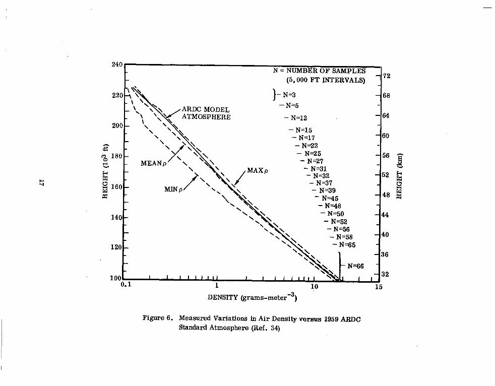
MRN data shows that large density variations exist over latitudinal and seasonal scales, increasing steadily as one moves upward and approaching a range of a factor of 2 at the 200,000 ft level. This condition is illustrated by Figure 6 which shows the minimum and maximum recorded densities above White Sands and Fort Churchill, Canada. Relative changes on a daily basis in upper atmospheric density are greater, by percentage, than annual sea level changes, and they approach the maximum observed at the surface.

3.3.1.1 Upper Atmospheric Winds. Above the North American continent, rocket data indicates that winds in the upper atmosphere exhibit a strong monsoonal tendency in all except equatorial regions. Summer conditions are relatively sedate in comparison with the winter circulation. Generally steady winds from the east, increasing gradually with altitude, are observed regularly throughout the summer season. These prevailing easterly winds achieve a speed of approximately 150 ft/sec during their peak strength in July. After July, there is a gradual decay in wind speed to a reversal in direction, which generally occurs in September. Peak winter winds generally occur in November and reach a peak of 150 to 300 ft/sec. During December and January a noticeable change in the data is evident. Large excursions become the rule, with a weakening of the strong westerly circulation in the general trend. The wind speed is observed to change at rates greater than 60 ft/sec per day and, on occasion, reverse for a few days to present the appearance of a typical moderate summer situation. After the strong January period the winds generally drop to a more sedate speed of 150 ft/sec through early April. The winds usually decrease during April and reverse in early May to the prevailing easterly summer state.

16

-

240/ I- N = NUMBER OF SAMPLES

(5,000 FT INTERVALS)

a20 - N=3 168

L- I - N=5

ATMOSPHERE - N=12 -64 I

200, 3 - N=15 - N=17 - 60 - N=22

180 - - N=25 - N=27

- N=31 - N=32

160 - - N=37 - N39 - N=45 - N--P8

140 - - N=50 -44

120 -

1 10 15 DENSITY (grams-meters3)

Figure 6. Measured Variations in Air Density versus 1959 ARDC Standard Atmosphere (Ref. 34)

4/CONTROL METHODS

4.1 CONSTANT L/D VEHICLES

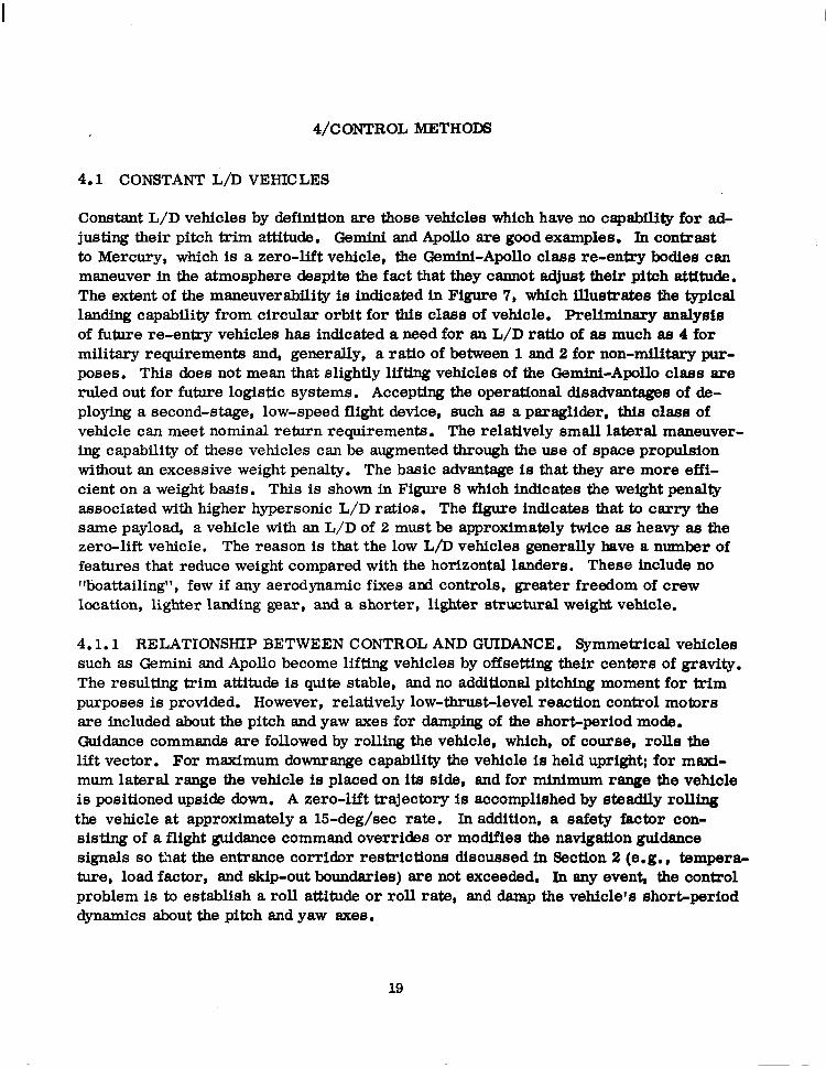
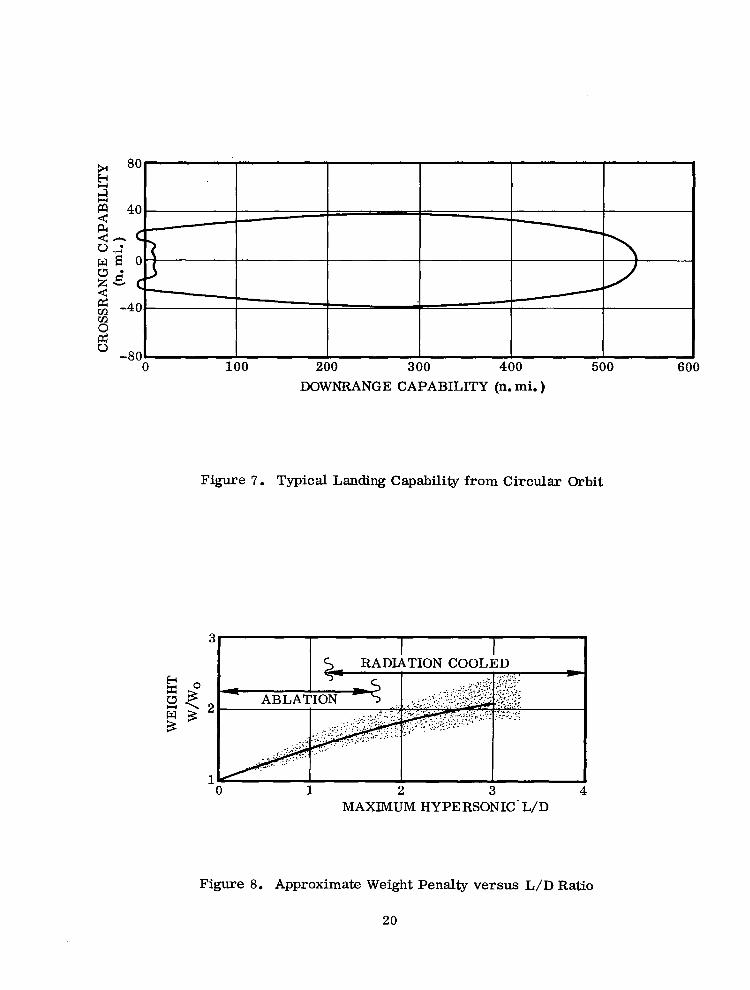
Constant L/D vehicles by definition are those vehicles which have no capability for adjusting their pitch trim attitude. Gemini and Apollo are good examples. In contrast to Mercury, which is a zero-lift vehicle, the Gemini-Apollo class re-entry bodies can maneuver in the atmosphere despite the fact that they cannot adjust their pitch attitude. The extent of the maneuverability is indicated in Figure 7, which fflustrates the typical landing capability from circular orbit for this class of vehicle. Preliminary analysis of future re-entry vehicles has indicated a need for sn L/D ratlo of as much as 4 for military requirements and, generally, a raUo of between 1 and 2 for non-military purposes. This does not mean that slightly lifting vehicles of the Gemini-Apollo class are ruled out for future logistic systems. Accepting the operational disadvantages of de- ploying a second-stage, low-speed flight device, such as a paraglider, this class of vehicle can meet nominal return requirements. The relatively small lateral msneuver- ing capability of these vehicles can be augmented through the use of space propulsion without an excessive weight penalty. The basic advantage is that they are more effi- cient on a weight basis. This is shown in Figure 8 which indicates the weight penally associated with higher hypersonic L/D ratios. The figure indicates that to carry the same payload, a vehicle with an L/D of 2 must be approximately twice as heavy as the zero-lift vehicle. The reason is that the low L/D vehicles generally have a number of features that reduce weight compared with the horizontal landers. These include no %oattailing”, few if any aerodynamic fixes and controls, greater freedom of crew location, lighter landing gear, and a shorter, lighter structural weight vehicle.

4.1.1 RELATIONSHIP BETWEEN CONTROL AND GUIDANCE. Symmetrical vehicles such as Gemini and Apollo become lifting vehicles by offsetting their centers of gravity. The resulting trim attitude is quite stable, and no additional pitching moment for trim purposes is provided. However, relatively low-thrust-level reaction control motors are included about the pitch and yaw axes for damping of the short-period mode. Guidance commands are followed by rolling the vehicle, which, of course, rolls the lift vector. For maximum downrange capability the vehicle is held upright; for maximum lateral range the vehicle is placed on its side, and for minimum range the vehicle is posiuoned upside down. A zero-lift trajectory is accomplished by steadily rolling the vehicle at approximately a 15-deg/sec rate. In addition, a safety factor consisting of a flight guidance command overrides or modifies the navigation guidance signals so that the entrance corridor restrictions discussed in Section 2 (e.g., temperature, load factor, and ship-out boundaries) are not exceeded. In any event, the control problem is to establish a roll attitude or roll rate, and damp the vehiclels short+eriod dynamics about the pitch and yaw axes.

19

-80 0 100 200 300 400 500 600

DOWNRANGE CAPABILITY (n. mi. )

Figure 7. Typical Landing Capability from Circular Orbit

3

0 1 2 3 4 MAXIMUM HYPERSONIC-L/D

Figure 8. Approximate Weight Penalty versus L/D Ratio

20

4.1.2 TYPICAL CONTROL SYSTEM. The attitude reference system for these vehicles is an inertial platform. Gemini has a four-ring gimbal assembly, while Apollo has only three, for added reliability;The measuring devices - three floated rate-integrating gyro and three orthogonal pulse-rebalanced accelerometers - are located on a stabi- lized inner block. ‘The addition of a fourth gimbal ring on Gemini, which is redundant in the roll axis, provides the vehicle with full 360-degree freedom about all three axes. There are two analog pickoffs on each gimbal ring of the platform to measure the angular difference between the vehicle and platform axes. Data from one set of ‘pickoffs is fed into a digital computer; data from the other set provides attitude reference information to the artificial horizon attitude indicator on the instrument panel. The pla+ form can be aligned in orbit in either a blunt-end-first or small-end-first mode. To accomplish this, the pilot must align the vehicle to 5 degrees of the horizon in pitch and roll, and 15 degrees in yaw with the platform in a locked or caged mode. The platform will align itself when uncaged by reacting its momentum vectors with the orbital rotation. This is called gyro compassing.

The autopilot provides an option of five different control modes during the re-entry maneuver. They are, in ascending order of complexity:

1. Direct - IIn this mode, steady-state firing of the thrusters occurs as long as the stick is deflected outside of its deadband area. Switches on the stick trigger the solenoid valve drivers on the thrusters.

2. Pulse - This mode triggers the attitude thrusters for 20 milliseconds. The stick must be returned to the neutral position after each pulse before a second pulse can be triggered.

3. Rate Command - Rate gyro signals are summed with the stick deflection in such a way that the vehicle is driven about its axes at a rate proportional to the amount of deflection in the attitude control stick. When the stick is returned to neutral, further turning is automatically damped out by the rate gyro signals.

4. Re-entry Rate Command - This is basically similar to the rate command described above, except that a deadband is included to reduce the thruster firing commands and thereby conserve the reaction control fuel.

5. In all the previous modes, the re-entry crossrange and downrange error signals, as supplied by the onboard computer, are presented to the pilot as needle deflections in front of the artifical horizon attitude indicator. By modulating the lift vector which the vehicle’s offset center of gravity provides, the crew will normally bank until the crossrange error is nulled. Then they will fly a maximum-lift trajectory until the downrange error also goes to zero, at which time the vehicle is placed in a steady 15-deg/sec roll which wipes out the lift. The vehicle then flies a ballistic trajectory to the landing site. In this mode, the pitch and yaw angular rates are automatically maintained within a certain deadband, and the roll rate is automatically controlled, based on the downrange and crossrange error signals as supplied by the onboard computer.

21

Both Gemini and Apollo reaction control systems use monomethyl hydrazine and nitrogen tetroxide thrusters. This fuel is a storable hypergolic combination. Gemini has 16 25-pound thrusters for attitude control. They are located at the small end of the vehicle and are grouped into two completely redundant sets of eight. The Apollo attitude control system has 12 loo-pound thrusters. Ten are located around the adapt- er rim and two are up near the small end. The system is completely dual for redundancy, and each thruster receives a pure pitch, roll, or yaw signal. The thrusters near the small end are for negative pitch.

4.2 VARIABLE L/D VEHICLES

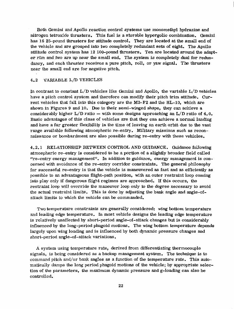
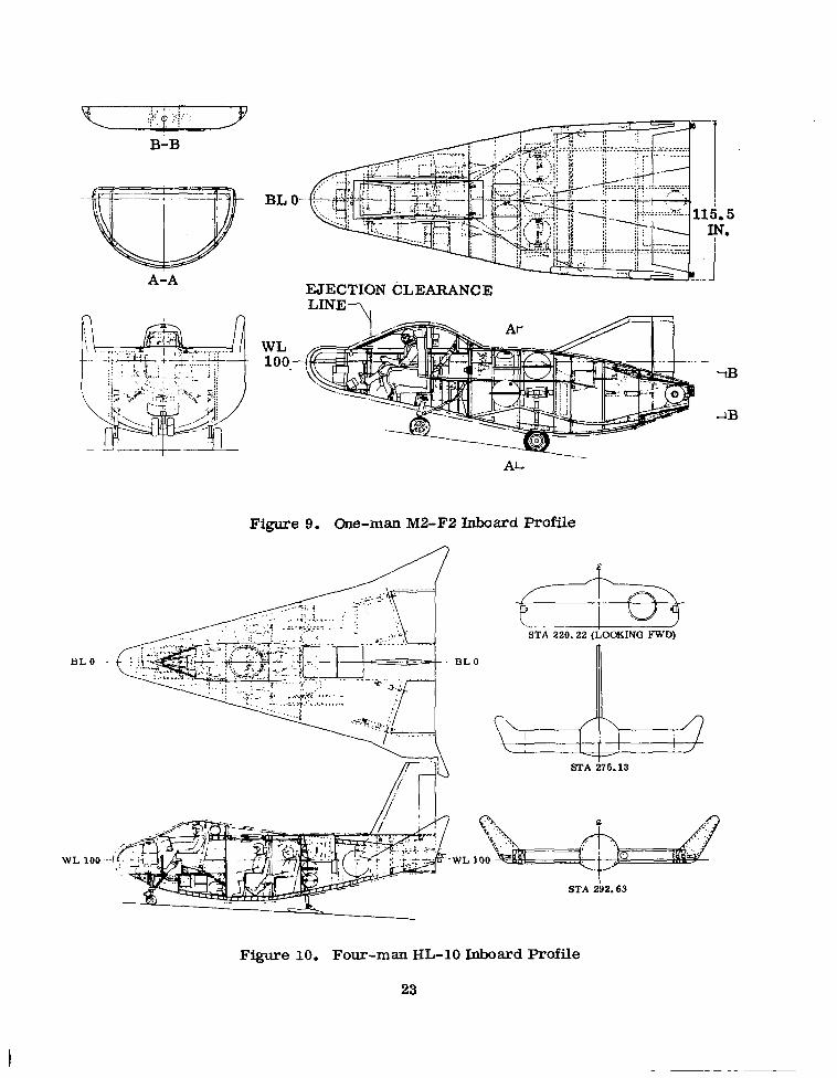
In contrast to constant L/D vehicles like Gemini and Apollo, the variable L/D vehicles have a pitch control system and therefore can modify their pitch trim attitude. Cur- rent vehicles that fall into this category are the M2-F2 and the HL-10, which are shown in Figures 9 and 10. Due to their semi-winged shape, they can achieve a considerably higher L/D ratio - with some designs approaching an L/D ratio of 4.0. Basic advantages of this class of vehicles are that they can achieve a normal landing and have a far greater flexibility in the time of leaving an earth orbit due to the vast range available following atmospheric re-entry. Military missions such as recon- naissance or bombardment are also possible during re-entry with these vehicles.

4.2.1 RELATIONSHIP BETWEEN CONTROL AND GUIDANCE. Guidance following atmospheric re-entry is considered to be a portion of a slightly broader field called IYe-entry energy management”. In addition to guidance, energy management is con- cerned with avoidance of the re-entry corridor constraints. The general philosophy for successful re-entry is that the vehicle is maneuvered as fast and as efficiently as possible to an advantageous flight-path position, with an outer restraint loop coming into play only if dangerous flight regimes are approached. If this occurs, the restraint loop will override the maneuver loop only to the degree necessary to avoid the actual restraint limits. This is done by adjusting the bank angle and angle-of- attack limits to which the vehicle can be commanded.

Two temperature constraints are generally considered: wing bottom temperature and leading edge temperature. In most vehicle designs the leading edge temperature is relatively unaffected by short-period angle-of-attack changes but is considerably influenced by the long-period phugoid motions. The wing bottom temperature depends largely upon wing loading and is influenced by both dynamic pressure changes and short-period angle-of-attack variations.

A system using temperature rate, derived from differentiating thermocouple signals, is being considered as a backup management system. The technique is to command pitch and/or bank angles as a function of the temperature rate. This automatically damps the long period phugoid motions of the vehicle; by appropriate selection of the parameters, the maximum dynamic pressure and g-loading can also be controlled.

22

B-B

AIA

BLO

BL O-

WL loo.-

.-._ .-__ ___. __.. .-_ . . . . . . ;: I-. .-...... L-l ; : ,, -.

EJECTIONCLEARANCE L~ET,

Figure 9. One-man M2-F2 InboardProfile

BLO

STA $75.13

STA 292.63

Figure 10. Four-manHL-10InboardProfile

23

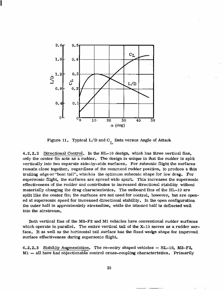
Generally, to extend the range, maximum L/D flight is required, and to decrease the range, maximum CL (lift coefficient) and possibly a large bank angle are required. Figure 11 illustrates typical L/D and CL data versus angle of attack for this class of vehicle. Note that. maximum CL occurs at an angle of attack of about 45 degrees. These guidance requirements have a direct influence on the control system. In particular, the handling criteria discussed in Section 2 must be met for these unusual vehicle attitudes.

4.2.2 TYPICAL CONTROL SYSTEM

4.2.2.1 Longitudinal/Lateral. The X-15, M2-F2, and HL-10 vehicles all combine the elevator-aileron function by having split trailing edge surfaces that operate differentially to perform the aileron function. The Ml vehicle, which is the plywood predecessor of the M2-F2, has independent ailerons outboard of the vertical fins; however, this design-was found to produce excessive dihedral which caused roll control difficulties during landing.

The M2-F2 longitudinal control system consists of upper and lower trailing-edge flaps. The upper flap (which is split to provide the aileron function) is controlled in the pitch ‘mode by a trim motor only. The primary pitch control actuates the bottom surface. The trim position of the bottom surface must be at some mid-deflection point to allow both positive and negative pitch control, without hitting the surface stops. This partial surface trim position is achieved by stick force trimming. The pilot’s pitch trim button, located on the stick, adjusts the force of a mechanical spring to counteract the aerodynamic forces on the surface for any desired surface position. Since both surfaces can be trimmed, there is a possibility that they can be inadvert- ently trimmed to oppose each other and produce a situation where insufficient lower surface motion is available to perform the flare maneuver. To guard against this possibility a panel meter is included to indicate to the pilot the positions of both the upper and lower surfaces.

In the HL-10, the trailing-edge surfaces that perform the elevator/aileron function are unusual because of their thickness. They generally follow the body shape and are approximately one-foot thick at the trailing edge. Attached to the surface on the top and bottom are auxiliary flaps that are opened during hypersonic flight to provide additional longitudinal stability and increased surface effectiveness.

The only movable flaps on the wings of the X-15 are conventional landing flaps. The elevator-aileron function is provided by fully movable and differentially operated, horizontal tail surfaces. Electrical control signals originating from the autopilot and/ or stability-augmentation systems have approximately the same authority as the pilot and are in series with his input. Failure-protection is supplied by redundancy and an electrical model of the actuator used to convert the electrical signal into a mechanical system input to the control system.

24

2. a

1.6

1.2 e I4

0.8

0.4

0

0.5

0.4

0.3

ti 0.2

0.1

r OO 10. 20 30 40 !

Figure 11. Typical L/D and CL Data versus Angle of Attack

4.2.2.2 Directional Control. In the HL-10 design, which has three vertical fins, only the center fin acts as a rudder. The design is unique in that the rudder is split vertically into two separate side-by-side surfaces. For subsonic flight the surfaces remain close together, regardless of the command rudder position, to produce a thin trailing edge or “boat tail”, whichis the optimum subsonic shape for low drag. For supersonic flight, the surfaces are spread wide apart. This increases the supersonic effectiveness of the rudder and contributes to increased directional stability without materially changing the drag characteristics. The outboard fins of the HL-10 are split like the center fin; the surfaces are not used for control, however, but are opened at supersonic speed for increased directional stability. In the open configuration the outer half is approximately streamline, while the inboard half is deflected.well into the airstream.

Both vertical fins of the M2-F2 and Ml vehicles have conventional rudder surfaces which operate in parallel. The entire vertical tail of the X-15 moves as a rudder surface. It as well as the horizontal tail surface has the fixed wedge shape for improved surface effectiveness during supersonic flight.

4.2.2.3 Stability Augmentation. The re-entry shaped vehicles - HL-10, M2-F2, Ml - all have had objectionable control cross-coupling characteristics. Primarily

25

these have been a yaw due to the action of the aileron and a roll due to that of the rudder. An adequate but simplified corrective measure consistent with the design objectives of the M2-F2 and HLklO, is to feed a roll rate signal tc the rudder. This is accomplished by tipping the yaw rate gyro (which normally supplies a damping signal to the rudder) away from the primary axis of the vehicle in such a way that it also senses a component of roll rate.

One of the three X-15 vehicles has an adaptive autopilot. This autopilot automatically blends in (starts) the reaction control motors when it determines that the aerodynamic control effectiveness is inadequate for proper control of the vehicle. All of the X-15 vehicles have side arm controllers located on the right-hand side of the cock- pit by which the pilot effectively flies the vehicle through the autopilot. The vehicles that do not have the adaptive autopilot have a left-hand controller to actuate the reaction control units. Pitch, roll, and yaw control are all built into the controller. Pitch and roll commands result from rotation of the controller, while yaw commands are produced by a lateral motion. Wing re-entry, the pilot operates both control systems, one with each hand. In the vehicle with the adaptive autopilot, reaction control pitch and roll are controlled by the right-hand stick along with aerodynamic pitch and roll, and reaction control yaw is controlled by the rudder pedals.

4.2.3 POSSIBLE PROBLEM AREAS. The following is a discussion of some of the problem areas that have been uncovered to date regarding the stability and control characteristics of variable-lift re-entry vehicles.

4.2.3.1 Lateral-Directional Stability. Mfficult problems of hypersonic lateral- directional stability were first encountered in the XlA and X2 aircraft. In December 1953 the XlA developed uncontrollable lateral oscillations at Mach 2.4. As a result, the aircraft was out of control for 70 seconds and lost over 10 miles of altitude before control was regained. The X2 on its last, fatal flight had the same difficulty. The trouble was traced back to loss of lifting effectiveness on the thin stabilizing surfaces and the resulting decrease in lateral stability. During development of the X-15 cal- culations indicated that a conventional vertical tail would have to be as large as one of the wings to maintain directional stability. The solution for the X-15 was the now familiar wedge-shaped tail. The advantage of the wedge shape can be seen by locking at the approximate formula for hypersonic lift on a flat plate, which is:

CN=- 2.8 sin2cW

and the practical derivative is

aCN - = CN au

= 5.4 sin o!

26

In other words, if there is a flow-incident angle at the trim position, as provided for by a wedge, the stability coefficient will be greatly increased. A refinement on the basic wedge shape is the variable wedge. This technique is used on the HL-10. The wedge is formed by split rudders that open like speed brakes. The advantage is that the wedge is available during hypersonic flight and can be modified to a thin surface for lower drag in the subsonic regime. Although the wedge shape has helped directional control considerably, the problem of instability is still present. Recent data on several possible re-entry configurations has shown directional instability at angles of attack required for maximum C at lower hypersonic speeds, which is a possible flight condition. The latest work 05 hypersonic vehicle criteria specifically states that positive directional stability is required for all permissible load factors.

With the conventional vertical tail location, the tail effectiveness in hypersonic flight csn decrease to zero with a particular angle of attack since the tail comes into the shadow of the body. This occurs on the upper tail of the X-15 at an angle of attack of about 20 degrees. To compensate for this, the X-15 was originally designed with a lower tail of the same size as the upper tail. The result produced good directional stability; however, the configuration had a negative dihedral effect, which is also an unacceptable handling characteristic. The reason for the negative dihedral effect was the marked increase in the effectiveness of the lower tail as a consequence of its penetration into the region of high dynamic pressure produced by the shock wave of the compression side of the wing. Consequently, the lower tail was reduced to 25 percent of its original area. Current re-entry configurations generally do not have lower tails. Instead, the vertical tails are placed where they are not easily shadowed by the body at higher angles of attack. The HL-10 and M2-F2 vehicles are examples of this approach.

4.2.3.2 Rudder Effectiveness. Rudder effectiveness is very closely connected to the lateral-directional stability control problems discussed above. In particular there exists the possibility that, for some configurations, the rudder or rudders can be in the shadow of the body for large angles of attack. Flight at high angles of attack including turns is required for certain situations in state of the art energy management techniques. In these situations it is likely that the rudder effectiveness must be sufficient to provide artificial yaw damping and assist in turn coordination.

4.2.3.3 Thermoelastic Effects. Re-entry vehicles will experience large differences in temperature, particularly between the upper and lower sections of the wing. Cn the X-15, this temperature difference is enough to cause a 15iinch upward deflection of the wing tip. Also, the high temperatures will have a substantial effect on the over- all bending stiffness. The result is a much greater deflection of the wing for the maximum g condition, and some difference in the bending modes. Because of this the control system design of surfaces and mechanisms should be checked for possible inter- ference or binding for hot vehicle bending deflections at the limit load factor. Also, body bending mode coupling into the autopilot for the hot vehicle will be more pronoun- ced, since the mode frequencies will be lower; this should be checked.

27

4.2.3.4 Vehicle Flexing. Vehicle bending modes can couple into an autopilot because the sensors (e.g., gyros and accelerometers) pick up not only the motion of the vehicles but the motion of the position of the sensor with respect to the total motion of the vehicle as well. Generally, the problem occurs with rate gyros and accelerometers because of the frequencies involved. Attitude gyro signals can be filtered to eliminate bending frequencies; however, this is usually not required. Re-entry vehicles will probably have adaptive rather than air-data-scheduled autopilots since the adaptive designs have the additional advantages of being able to compensate for uncertaim&s in the vehicle’s aerodynamics. The X-15 has such a system. In it, a number of changes in system gains and compensation networks as well as the addition of notch filters were required to prevent coupling between the self-adaptive flight control system and bending modes.

The state of the art for stabilizing or preventing instability of the elastic modes consists of three basic means. These consist of cancellation, phase-stabilization, and gain-stabilization. Cancellation consists of eliminating the bending mode signal from the sensor feedback, either by proper location on the vehicle, multiple sensors, or by some other method. Phase-stabilization is the provision of proper phase characteristics so that the feedback bending signal has a stabilizing effect. Gain- stabilization results from reduced gain of the flight control system at the frequency of bending mode due to the natural bandpass of the system or special filtering. Of the latest techniques the most promising are listed below.

a.

b.

C.

Rate-Gyro Blending. This method blends the signals from two gyros, one located forward of and the other behind the first bending mode antinode. The ratio of the gains of the two rate gyros is automatically adjusted to cancel or give the proper phase relationship to the first bending mode.

TrackingNotchFilters. This is a technique of automatically tracking and rejecting -- the bending mode signal. A frequency-sensing system determines the bending mode frequency and controls a variable notch filer.

Multiple Sensors. This method uses multiple rate gyros, generally 6 to 10, located at particular points along the vehicle. By proper location of the gyros and adjustments of the gains the bending modes can effectively be eliminated. The system also provides a degree of redundancy.

4.2.3.5 Control Cross-Coupling. Re-entry vehicles have substantial control cross- coupling. For instance, data from a current configuration indicates a yaw due to the aileron moment coefficient, C

%a’ approximately equal to l/2 of the roll due to the

aileron moment coefficient, CQ . Even worse, the pitching moment coefficient due 6a

28

to rudder action, C m6R’

is three times as great as the yawing moment coefEicient due

to rudder, Cn . In general, the ailerons will produce a yawing and pitching moment 6R

in addition to the rolling moment; and the rudder will give rolling and pitching momenta as well as the yawing moment. A particularly bad control cross-coupling situation is for the ailerons to produce, in addition to a positive rolling moment, a negative yawing moment. Eggleston, Baron, and Cheatham (Reference 7) conducted a re-entry simulation program that included control cross-coupling. Using relatively large, but possible, cross-coupling parameters, they found that partial or total loss of control resulted, particularly when vehicle damping was light.

4.3 EXPERlMENTAL CONTROL TECHNIQUES

The following devices have not aa yet been reduced to practical eyeterns; however, they indicate trends and possible future advances in the state of the art of controlling re-entry vehicles.

4.3.1 MOVABLE NOSE SPIKE; This device was conceived at Wright-PattersonAFB Aerospace Research Laboratories. The idea is to develop controllable pitch and yawing moments by means of a nose-mounted spike. The attitude of the spike with respect to the vehicle is controllable and the moment is proportional to the deflection angle. Spike ablation is a major problem. Suggested solutions are to lengthen tbe spike from within the vehicle or to use a liquid- or gas-cooled spike. Interesting advantages of the spike control system are that it would reduce the drag of the vehicle by about 10 to 16 percent and reduce the heat transfer to the nose cone.

4.3.2 MAGNETOHYDRODYNAMIC FLIGHT CONTROL. At hypersonic velocities a high-temperature, ionized shock layer exists about the forward porttons of a re-entry vehicle. Since this shock layer is an electrically conducting fluid, a magnetic field generated in the vehicle will react against it and produce a controllable force. The invisioned control system consists of an electromagnet and electrodes installed in the nose of the re-entry vehicle. Reversing the direction of the electric or magnetic fields reverses the direction of the control forces. Alternately, an electromagnet which can be swiveled about its center to some angle of attack to the flow direction can be used. The feasibility of this form of control system has been investigated by analysis and wind tunnel studies. The results are generally promising, particularly because of the recent discovery of high field strength super-conducting magnetrr, which require only the power necessary to maintain the cryogenic environment.

The reason magnetohydrodynamic control is being considered is that no external vehicle geometry changes (such as aerodynamic flaps) are required during re-entry. Instead, the magnetic and/or electric field acts as an invisible flap which extends in- to the flow, interacting with the ionized fluid and in turn producing a reaction at iti

29

source - the magnet onboard the vehicle. Thus the difficulties of heating and mechanical operation of conventional aerodynamic surfaces at hypersonic flight would be eliminated.

4.3.3 VARIABLE-DRAG DEVICES. The re-entry vehicle must be capable of staying within its operational envelope but still be able to change its flight condition (e.g., values of trim, lift and drag) at thediscretion of the pilot in order to control range. This is because the control of rate of change of velocity and altitude, or the ratio of kinetic to potential energy while energy is being dissipated, determines the total range of the flight and the point of landing. All variable-lift vehicles have a degree of variable drag, since changes in trim angle of attack cause drag as well as lift variations. However, desired changes in velocity and glide path angle may not be achiev- able in this manner for some configurations.

Proposed variable-drag devices include the split-rudder design of the HL-10, that opens like a conventional speed brake, and drag parachutes.

4.3.4 AUGMENTED MINIMUM SYSTEMS. Some of the vehicle-alone dynamic characteristics discussed in Section 4.2.3 are unsatisfactory from the standpoint of desirable handling qualities. But few high-performance craft have completely satisfactory vehicle-alone dynamics, and the problem of making the effective dynamics tfgoodtf gives the flight control ‘control designer a basis for the selection of feedbacks to correct the deficient dynamic characteristics.

of much greater significance to future manned entry vehicles is the possibility that the vehicle-alone dynamics are likely to be incapable of meeting even absolute minimum handling qualities. Specifically, the directional divergence indicated for high angles of attack is beyond pilot control capabilities. In the past, such situations have been eliminated by configuration changes, either fixed or variable in flight, or have been avoided by limiting the performance envelope. Based upon what is now known or suspected about the probable dynamics of lifting hypersonic entry configurations, the first of these possibilities is unlikely, and the second may restrict the entry corridor to unrealistically small limits.

A possible approach to alleviating the static instability problem is to rely on the augmentation system. Stability-augmentation systems that control unstable missiles are common. This solution has been avoided for manned aircraft because the reliability of static structures is-superior to that of electronic augmentation systems. Reliance has accordingly been placed upon one or the other of the fixes already noted. But with current re-entry vehicle configurations, such measures may no longer be sufficient. To meet the reliability desires, the primary system and any possible “residual” system should have a composite reliability index, based upon two independent failures, which is comparable to that of the vehicle structure. The present state

30

of the art appears to be at or near the point where such reliability levels can be achieved with properly dualed’and otherwise redundant systems.

4.4. UNMANNED RE-ENTRY VEHICLES

To date the most sophisticated vehicle which re-enters the atmosphere under automatic control is Asset. This vehicle is designed to evaluate the hypersonic lifting characteristics of a typical re-entry configuration. The 1200-pound vehicle has a total lifting area of 14 square feet and an unusually high density, approximately equal lx3 that of sea water. Operationally, the vehicle is boosted into a sub-orbital flight along the Atlantic Missile Range by a two-stage Thor rocket.

The Asset vehicle’s flight-stabilization system consists of three rate-integrating gyros as an angular reference package and three rate gyros to provide damping. Roll and pitch attitude programmers are also included. Reaction control motors provide the control forces; they use pressurized hydrogen peroxide which expands as a result of catalytic action at the motors to produce high-pressure steam and oxygen.

The Asset vehicle has a rather unique method of modifying its pitch trim attitude. The technique is to shift the center-of-gravity location by pumping liquid mercury between forward and aft tanks. The complete transfer of the mercury will shift the trim angle of attack about 15 degrees and can be done in 45 seconds. The amount of mercury is 30 pounds, which is sufficient to move the center of gravity 1.2 inches.

Electrical power for the flight-stabilization system is provided by rechargeable silver-zinc batteries. All wiring is insulated by teflon to provide temperature protection to 400°F, and bundles of wiring are wrapped in fiberglass tape for abrasion protection. In addition, redundant wiring techniques are employed.

Unmanned vehicles require some form of flight termination system to prevent possible impact damage to an inhabited area. Cn the Asset vehicle, flight termination is accomplished by severing the left wing with a shaped charge. The result of this action is a high rolling velocity and a predictable ballistic flight path. Since communications with the ground station can be interrupted by plasma effects around the vehicle during re-entry, the destruct logic is carried aboard the vehicle. For the Asset vehicle, the destruct logic is a roll angle in excess of a preselected value, or a loss of electrical power.

31

5 /ANALYSIS

&-entry vehicles when disturbed from an equilibrium flight path have been shown ana- lytically to exhibit characteristic oscillatory motions which may be identified with those of a conventional airframe. That is, there is a characteristic long-period motion in which the velocity, pitch angle, and altitude vary periodically, while the angle of attack remains essentially constant. There is a characteristic short-period motion in which the angle of attack and pitch angle vary periodically while the velocity remains essentially constant. Re-entry vehicles differ from conventional aircraft in that the period of the so-called “short-period” motion increases greatly at extreme altitude and may degenerate into a simple divergence at some high altitude.

Both the long- and short-period dynamics are analyzed on the basis of small disturbances from the equilibrium or non-oscillatory re-entry flight path. This leads to linear differential equations with time-varying coefficients since conditions along the flight path vary. The solution to these equations can be approximated by Bessel functions since the rapidly increasing atmospheric density as the vehicle descends through the atmosphere causes the aerodynamic restoring moment to act as a stiffening spring. Thus, the oscillation must decrease in amplitude and increase in frequency, which is precisely the behavior described by the Bessel function. (The analysis leading to the Bessel function solution is given in Section 5.2.)

A further simplification is made in order to analyze a specific re-entry vehicle- autopilot configuration. This is to assume that the changes in aerodynamic coefficients and dynamic pressure occur slowly with respect to the short-period motions of the vehicle. The time-varing coefficients in the linear differential equations thus become constant, and the designer can use the wide field of linear stability analysis techniques that are available. The development of these linear, constant coefficient differential equations is presented in Section 5.1.

5.1 SMALL PERTURBATION EQUATIOKS

The usual method for investigating the stability and control characteristics of either an aircraft or a re-entry vehicle is to investigate the response of the vehicle when it is disturbed a slight amount from a trimmed attitude. (Figure 12 exhibits the vehicle coordinate system.) The reason is that the equations for the aerodynamic forces and moments, as well as the D’Alembert forces and moments can be considered linear. The expansion and linearization of the D’Alembert or inertial terms is available in most standard texts on aircraft dynamics. Reference 33 is particularly clear and complete. It develops the rigid body equations of motion, taking into account the situation where the geometric center and mass center do not coincide. The major assumptions in this reference are that the earth’s position is fixed in inertial space and the

33

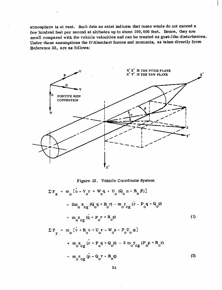
atmosphere is at rest. Such data as exist indicate that mean winds do not exceed a few hundred feet per second at altitudes up to about 100,000 feet. Hence, they are

small compared with the vehicle velocities and can be treated as gust-like disturbances. Under these assumptions the D’Alembert forces and moments, as taken directly from Reference 33, are as follows:

X’ 2’ IS THE PITCH PLANE X’ Y’ IS THE YAW PLANE

Figure 12. Vehicle Coordinate System

GF = mo[u- X

Vor + Woq + Uo(Qo~-RoB)l

- 2mo xcg (Q,q + Ror) - moycg 6 - Poq - Qop)

+ mozcg (i + Par + Rap) (1)

. GF =

Y * mo[v+Rou+U r-Wop-PoUoaI

0

+ mx 0 cg

(i + P$’ + Qop) - 2 moycg (Pop + Ror)

- moZcg 6 - Qor - RoO (2)

34

xFZ = mocw+Vop-Qou-Uoq+Pouo~]

- moxcg (;1- Par - RIP) + moycg (p + Qor + Ro4)

- 2 m. zcg (Pop + Q,Q

CM x = 12 + (Izz - Iyy’ (Qor + Bog’ - Ixy <i - PO’ - Rap)

- 1% 6 + Poq + Qop) - 3 Iyz (Ror - Q,4)

+mY 0 w (; + Vop - Qou - Uoq + PoUoB)

- mz 0 w

(; + Rou + Uor - Wop - PoUoa)

CMy = (Is - Izz) (PO’ + Rap) + Iyy q - Ixy (p + Q,r + Roq)

- I~ (i - PO9 - Qop’ + 2 Ixz (pop - Ro”

- mx 0 cg

6 + Vop - Qou - Uoq + PoUoB)

+ mozcg[u-Vor+Woq+Uo(Qoa!-RoBI

CMZ = (I YY

-Ixx)(Poq+Qop)+I zz r -I,(p-Q,r-Roq)

_ ryz (i + Par + Rap) + 3 I xy (Q,s - POP)

+ mx 0 w

(; + Rou + Uor - Wop - PoUo ar)

- moycg[;-Vor+Woq+Uo(Qo~ -Rob)]

(3) ..:

(4)

(5)

(6)

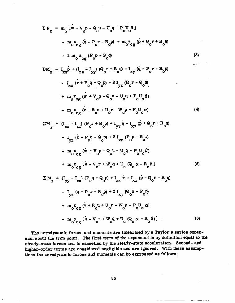
The aerodynamic forces and moments are linearized by a Taylor’s series expansion about the trim point. The first term of the expansion is by definition equal to the steady-state forces and is cancelled by the steady-&ate acceleration. Second- and higher-order terms are considered negligible and are ignored. With these assumptions the aerodynamic forces and moments can be expressed as follows:

35

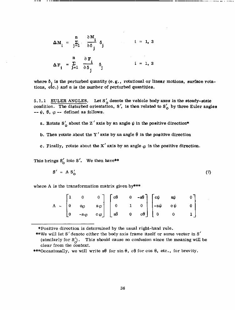
n aM.

AMi = jgl’ -2 6. a6

j '

i = 1,3

i = 1, 3

where 6. is the perturbed quantity (e. g. , rotational or linear motions, surface rota- tions, e ic.) d an n is the number of perturbed quantities.

5.1.1 EULER ANGLES. Let Sb denote the vehicle body axes in the steady-state condition. The disturbed orientation, S’, is then related to Sd by three Euler angles --St 0, cp -- defined as follows.

a. Rotate Sb about the Z ’ axis by an angle $I in the positive direction*

b. Then rotate about the Y’ axis by an angle 8 in the positive direction

c. Finally, rotate about the X’ axis by an angle cp in the positive direction.

This brings SL into S’. We then have**

S’ = AS;

where A is the transformation matrix given by***

(7)

*Positive direction is determined by the usual right-hand rule. **We will let S’ denote either the body axis frame itself or some vector in S’

(similarly for SJ . This should cause no confusion since the meaning will be clear from the context.

***Occasionally, we will write se for sin 8, cCI for cos 8, etc., for brevity.

36

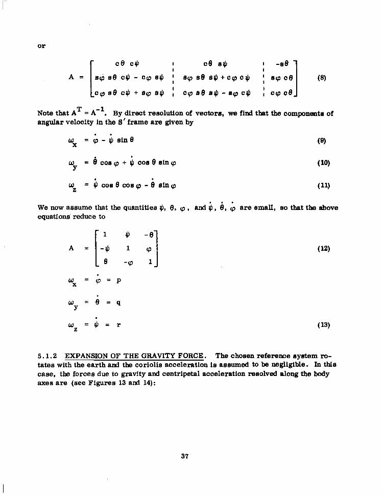
or

A= I (8)

T . NotethatA- =A-? By direct resolution of vectors, we fixxl that the components of angular velocity in the S’ frame are given by

0 X

= ;, - $I sin 8 (0)

WY = 6 cOSQ + $ CO08 SfnQ (10)

w Z

= 4 COB 8 COB Q - i sin Q (11)

We now assume that the quantities 9, 8, cp, and 6, 6, tjj are small, so that the above equations’ reduce to

[ 1 9 -8 A = -9 1 Q, 1 (12)

8 ‘Q 1

wX z&p

w Y =i=q

0 Z

=$= r (W

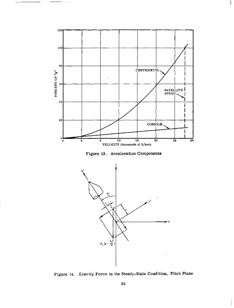
5.1.2 EXPANSION OF THE GRAVITY FORCE. The chosen reference system ro- tates with the earth and the coriolis acceleration is assumed to be negligible. In this case, the forces due to gravity and centripetal acceleration resolved along the body axes are (see Figures 13 and 14):

37

_._ _.-..-- .----

120

100

60

;M

8

g 60

ri 2

40

20

0- 0

CENTRIPETAL

I , a 12 16 20

VELOCITY (thousands of ft/sec)

Figure 13. Acceleration Components

VC2 M,(K- ~1

I

Figure 14. Gravity Force in the Steady-State Condition, Pitch Plane

38

F(O) xg

co9 e.

F(O) sin 8 xi3 0

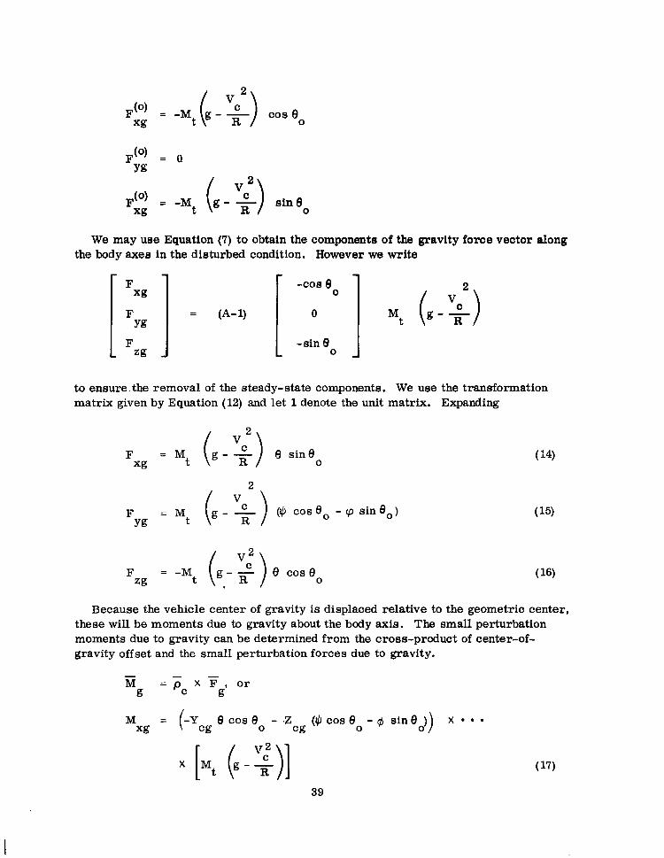
We may use Equation (7) to obtain the components of the gravity force vector along the body axes in the disturbed condition. However we write

to ensure. the removal of the steady-state components. We use the transformation matrix given by Equation (12) and let 1 denote the unit matrix. Expanding

F 9 sin8 xg 0

F Yg

(2) coseo -cp sineO)

F 8 co9 9 zg 0

( 14)

( 15)

(16)

Because the vehicle center of gravity is displaced relative to the geometric center, these will be moments due to gravity about the body axis. The small perturbation moments due to gravity can be determined from the cross-product of center-of- gravity offset and the small perturbation forces due to gravity.

ii g = K x 5’ Or 8 co9 8 - z

cg 0 cg (@costlo-g singo)) X l **

X [Mt (g-z)] 39

( 17)

M = Ylz

(+ z w

8 sine0 + x w

M zg

= C- ycge sine0 + x cg (G ~0~ 8

0 -@ sineO)] x . . .

t

(18)

(W

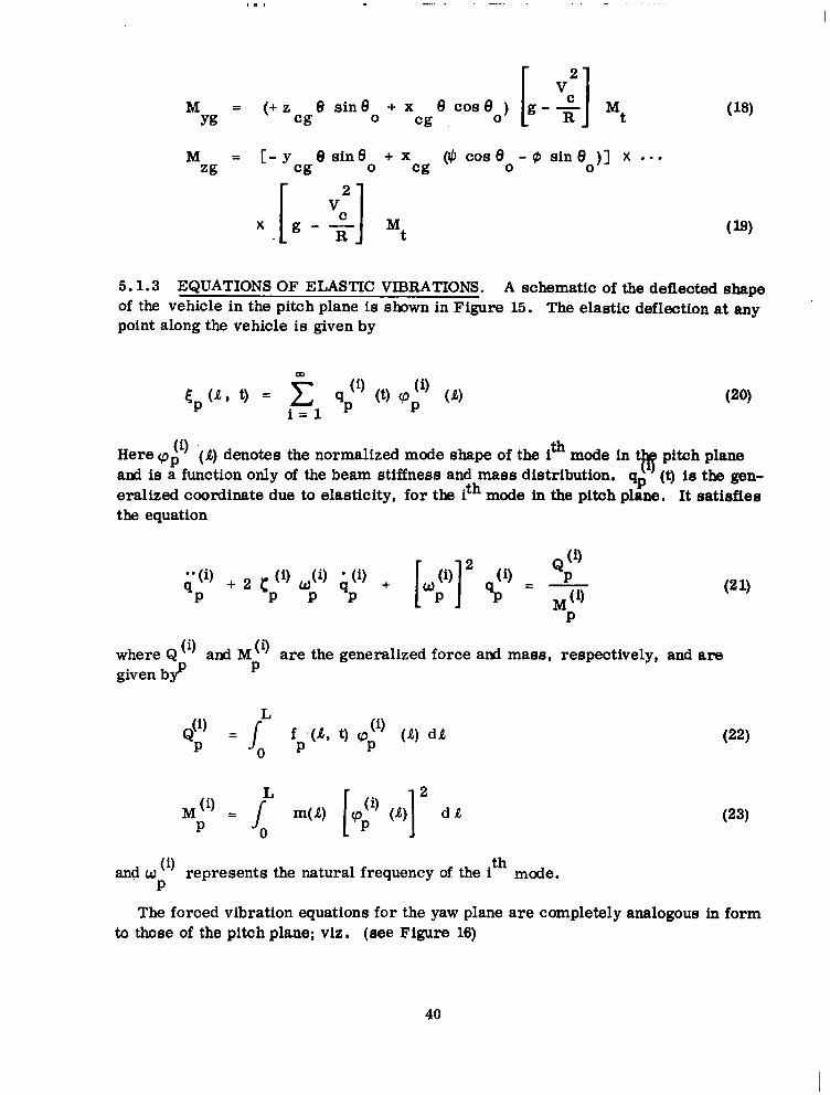
5.1.3 EQUATIONS OF ELASTIC VIBRATIONS. A schematic of the deflected shape of the vehicle in the pitch plane is shown in Figure 15. The elastic deflection at any point along the vehicle is given by

5, (a, t) = 2 pp”’ (t) Q;” (a) i=l

(20)

Here Q:) (a) denotes the normalized mode shape of the ith mode in t# pitch plane alld is a function only of the beam stiffness and mass distribution. qp (t) is the generalized coordinate due to elasticity, for the ith mode in the pitch plane. It satiefies the equation

;; (0

P P

where Q (i) and M(i) given byp P

are the generalized force and mass, respectively, and are

2 d.&

(21)

(22)

(33)

and w O) i th

mode. P

represents the natural frequency of the

The forced vibration equations for the yaw plane are completely analogous in form to those of the pitch plane; viz. (see Figure 16)

40

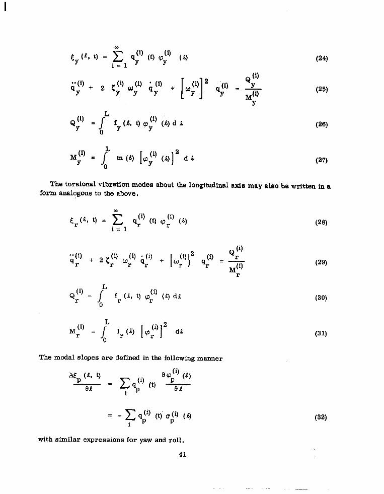
i$, ta, t) = 2 q; (t) Q; (a) (24) i=l

Q(‘) = L

Y J 0

fy (a, t) Q;’ ii) d a

(37)

The torsional vibration modes about the longitudinal axis may also be written in a form analogous to the above,

p

r

Q li)

r

(A, t) ,P(~) (k) dR r

Mti) = r /” 1r (A) [ $)]” d.8

0

The modal slopes are defined in the following manner

c q(i) (t) aQ;‘) (a)

aa = i ’ aa

= - c i

qj’) (tj c$) (a)

C-33)

(39)

(30)

(31)

(33)

with similar expressions for yaw and roll.

41

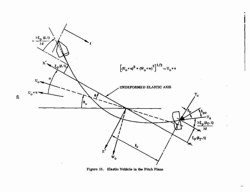
[ (uo+u12 + w,+w 2 m 1 do+u

UNDEFORMED ELASTIC AXIS

Figure 15. Elastic Vehicle in the Pitch Plane

Y’

Figure 16. Elastic Vehicle in Yaw Plam

5.2 VARIABLE DENSITY SOLUTION

The following analysis generally follows the work reported in References 10 through 22. The solutions describe the characteristic osciUations of a re-entry vehicle with controls fixed and subject to some form of initial disturbance. The equations are similar to the small perturbation eolution developed in the preceding section except

‘that atmospheric density is treated as an exponential function of altitude rather than as a constant. Since the solutions are linear equation6 with time-varing coefficients, they are generally not used for closed-loop stability analysis of the autopilot-vehicle configuration. Several investigators have recently pubDeW technique8 for analyzing TVP (time-varyingparameter) systems; however, the difficulty in applying’the techniques to a particular engineering problem has prevented their wide acceptance. Gib- son (Reference 23) gives a good presentation of the latest work in this field. In addition to their possible use in closed-loop stability analysie, the eolutions aid in understand- ing the re-entry control problem iir that they show the pneral characteristics of the oscillating motion. For instance, the solution pointa out that the maximum angle of attack of a vehicle descending through the atmosphere at a relatfvely constant speed is reduced. even without aerodynamic damping.

5.2.1 EQUATIONS OF MOTION, Beferring to Figure 17 oad using the nomenclature shown on the figure, the summation of force8 along the flight path; the summation of forces perpendicular ter of gravity lead to

mir = qA

.

to the flight path, and the summation of momenta about t& &en- the folIowing set of equations.

CD + nig sin yt

mVyt= -qACL + CO8 y t

16 =qARCCm

CC m = C=“t+ $ cm; &, + 1 c

V mq 6

(33)

(34)

Two distinot type8 of motion are represented by theBe equation@, One 10 the approximate trajectory of the vehicle’s center of gravity; the other ir ths oscillation of ths vehicle about ite center of gravity alid the oscillation of the center of gravity about the approximate or nominal trajeotory. The two types of motion are eeparated from eaoh other by assuming that the oscillatory motion consists of small perturbations about the nominal trajectory. This is done by making the following substitutions:

44

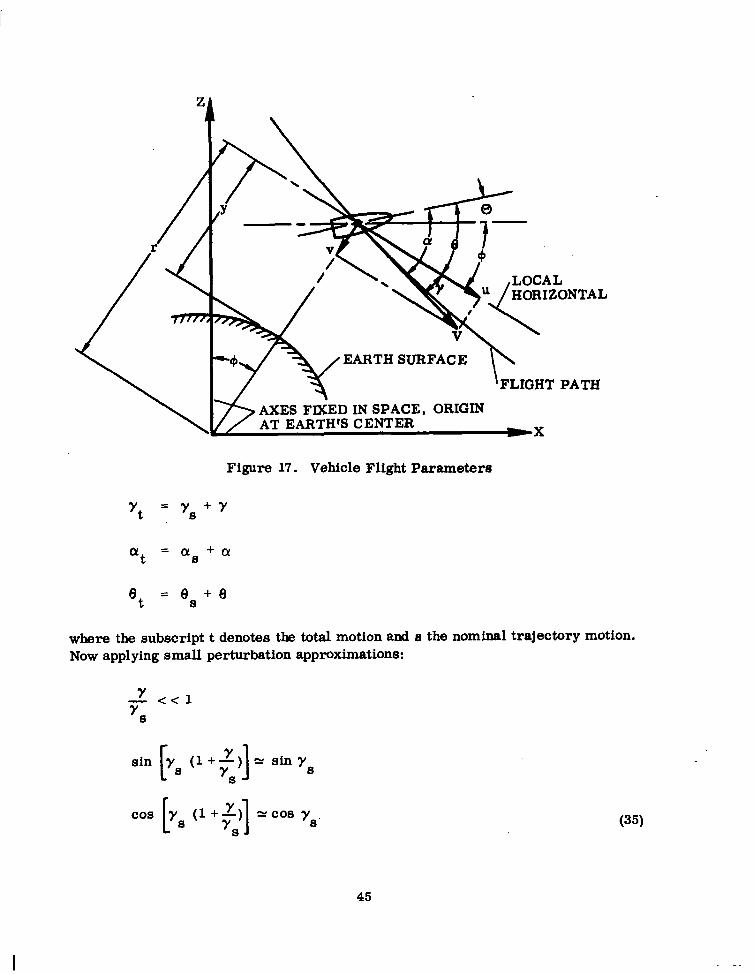
EARTH SURFACE

FLIGHT PATH

’ Au /HORIZONTAL

Figure 17. Vehicle Flight Parameters

Yt = y,+y

“t = cYg+cY

where the subscript t denotes the total motion and s the nominal trajectory motion. Now applying small perturbation approximations:

r <<l ys

sin [ys (1 +<)I = sin Y,

co9 [Ys (1 +J$] ‘ycos y,. (35)

45

I

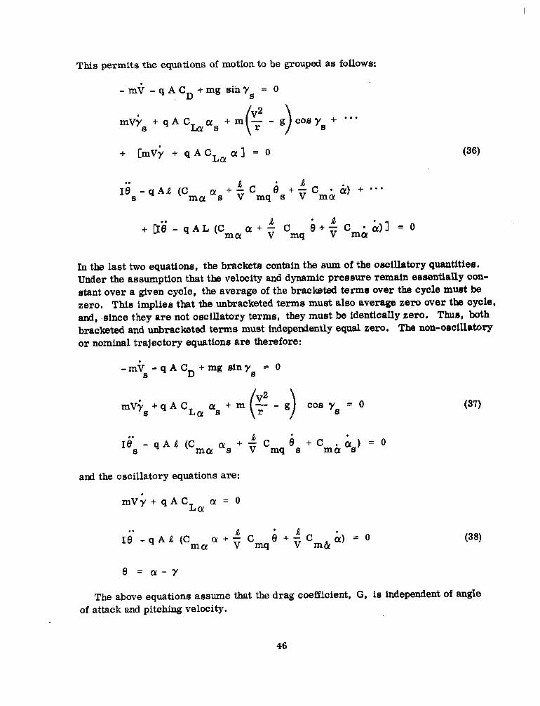
This permits the equations of motion to be grouped as follows: .

-mV -q+ +mgsiny = 0 S

rnV+ +qAC S

. + [mVy + qAC La!al = 0 (36)

1es AC -qAR (CmoLos+y mq~s++Cm&~) + . . .

+ CI’e’ - qAL (CmaQ + v ac i+ mq

+&&)I =o

In the last two equations, the brackets contain the sum of the oscillatory quantities, Under the assumption that the velocity and dynamic pressure remain essentially constant over a given cycle, the average of the bracketed terms over the cycle must be zero. This implies that the unbracketed terms must also average zero over tbs cycle, and, .since they are not oscillatory terms, they must be identically zero. Thus, both bracketed and unbracketed terms must independently equal zero, The non-oscillatory or nominal trajectory equations are therefore:

-mG s-qACD+mg sinys = 0

rnVi, + q A C

IKs - qAa(CmOros+T mqt$+Cm&&a) =0 5 *

and the oscillatory equations are:

mVj+qAC LCY

a=0

Iif .

-qAR (%P + kc e+ V mq a, ;y)=O V mh 8 = a-y

(37)

(36)

The above equations assume that the drag coefficient, G, is independent of angle of attack and pitching velocity.

46

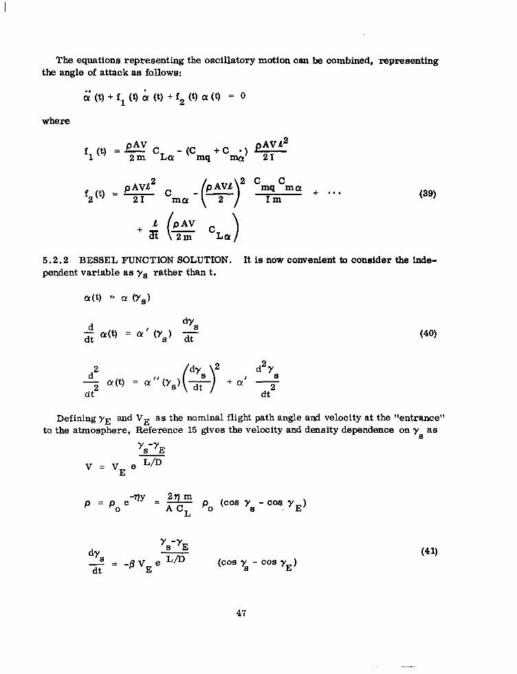
The equations representing the oscillatory motion csn be combined, representing the angle of attack as follows:

tit- (t) + f, (t) ; (t) + f2 0) 01(9 = 0

where

fl w =

f2 U) =

P AV 2m CLCY - (Cmq + C&l

p AW2 21

C ma

pAVd2 21

c c mq ma

Im + . . . WV

5.2.2 BESSEL FUNCTION SOLUTION. It is now convenient to consider the independent variable as ys rather than t.

a(t) = a (Y,)

$ o!(t) = ““YJ d’S

dt

2 A- o!(t) = cl!” (Y,) dt2

+ CY’

(40)

d2Y S

dt2

Defining YE and VE as the nominal flight path angle and velocity at the “entrance” to the atmosphere, Reference 15 gives the velocity and density dependence on ys as

‘s-‘E V = VE e L/D

p = p, e-” = AF p. (cos ys - COB YE) L

d’S

‘s-‘E

dt = -6 vE e L/D &OS Y

S - cos YE’

(41)

47

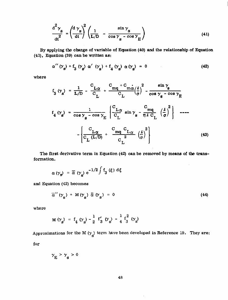
siny S

COB y - COB Y S E

(41)

By applying the change of variable of Equation (40) and the relationship of Equation (41), Equation (39) can be written as:

a” (Y,) + f3 cr,, a’ CY& + f4 CYs) a <Ys) = 0 w where

C f3(Ys) =$5- + +

C +c ’ 2

L mqc

ShY

L ma(%) -cosy -Bcosy

6 E

f4 (r,) = cosy 8

_‘cos y E

1 C Lot

- cL(LD) +

I C LCY C siny mq A2 - - -

cL 8 qla CL 0 ---- ()I

c c mq La

2 A

2 01 0 (43)

cL

The first derivative term in Equation (42) can be removed by means of the transformation.

0~ (Y,) = E Cr,) e -112 / f3 (5) d5

and Equation (42) becomes

Y" (ys) + M Cr,, i5i (Y,) = 0 (44)

where

1 2 M (r,) = f4 (Y,, - ; f’3 (Ys) - 4 f3 (Ys)

Approximations for the M (Y$ te rm have been developed in Reference 19. They are:

for

48

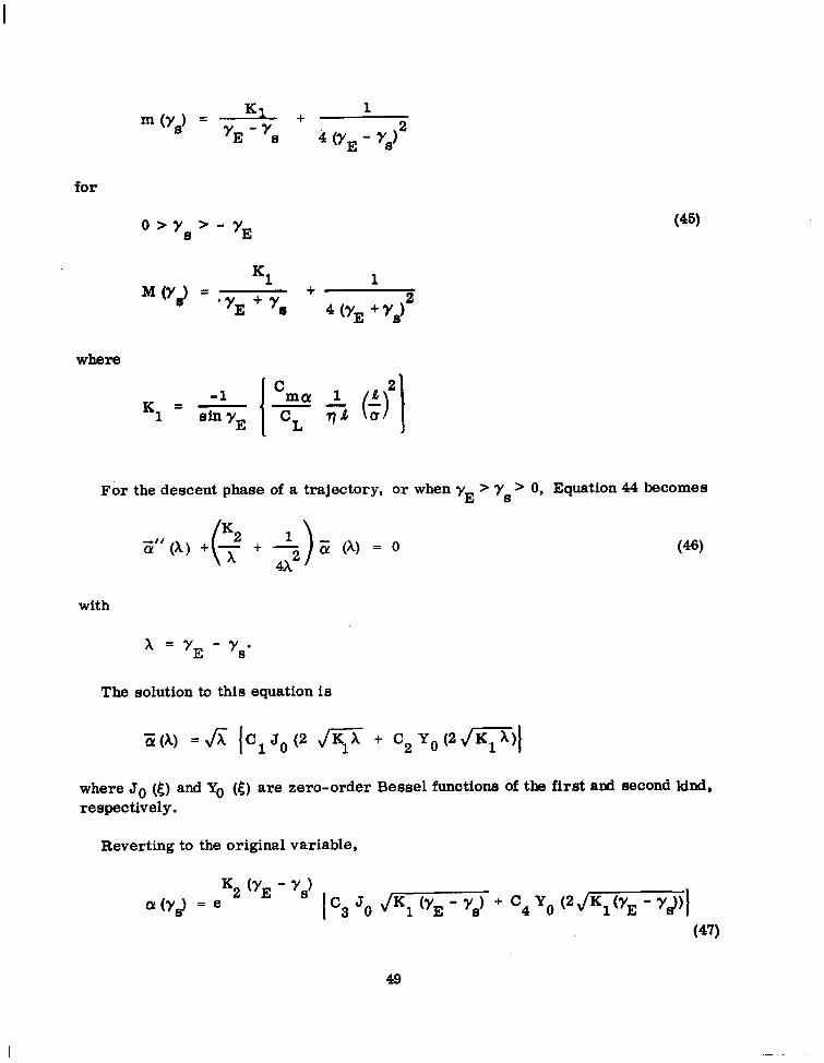
K1.. 1 m ‘YB’ =

YE O’S 4 (YE - Ys12

for

0 > Y, ’ - YE

K1 1 +y +

E s 4 (YE + Ys12

(45)

-1 C ma 1 A2

K1=- -- - sin yE i

C L 4 rlJ a

For the descent phase of a trajectory, or when yE > ys > 0, Equation 44 becomes

Z”(x) j(: + 2) z (A) = 0 (46)

with

x = YE - y * S

The solution to this equation is

z(A) =fi jC1Jo(2 m + C2yo(2~)I

where Jo (5) and Y. (5) are zero-order Bessel functions of the first and second kind, respectively.

Reverting to the original variable,

a tr,> = e K2 (‘E - YJ

I ‘3 JO JK1 (‘E - Ys’ + c4 y() (2 - ys))l (47)

49

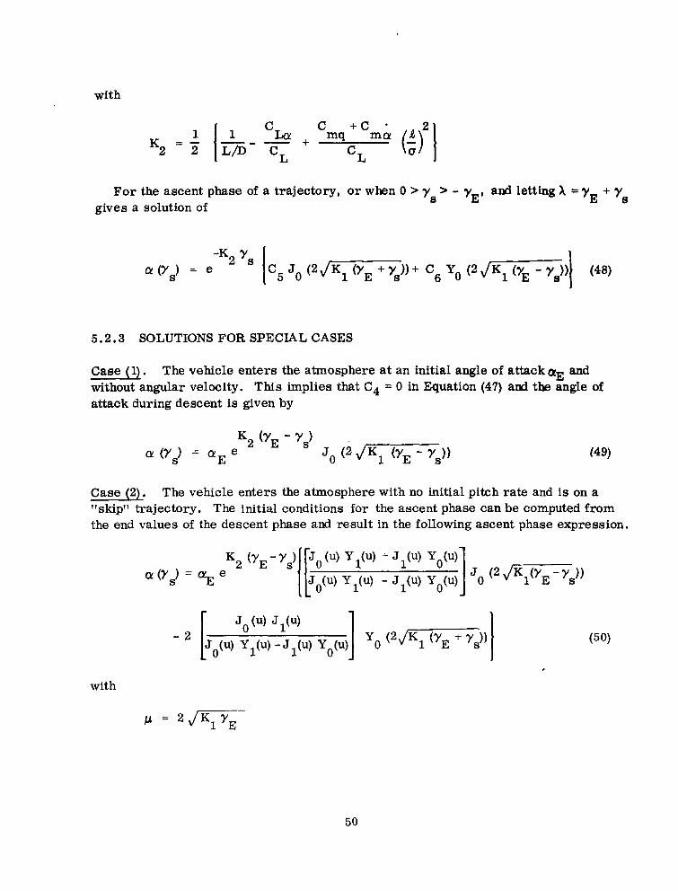
with

K2 = ; I

1 %cy cmq+cm& L/D--q + cL

For the ascent phase of a trajectory, or when 0 > y, > - YE, and letting X = yE + ye gives a solution of

a (Y,) = e -K2 Ys

I C5 Jo (2 d-1) + C6 Y. (2 d-1

I (48)

5.2.3 SOLUTIONS FOR SPECIAL CASES

(1). Case The vehicle enters the atmosphere at an initial angle of attackaE and without angular velocity. This implies that C4 = 0 in Equation (47) and the angle of attack during descent is given by

K2 ‘yE - ys) CY (YJ = aE e Jo l2 JK1 ‘YE - r,,, (49)

lu 1 Case (2). The v e ‘c e enters the atmosphere with no initial pitch rate and is on a l’skipV’ trajectory. The initial conditions for the ascent phase can be computed from the end values of the descent phase and result in the following ascent phase expression.

a Vs) = % e K2 WE - ys)

I Jo (2 dv;,,

-2 Jo 04 JIW Y,(u) - JIW Y,(u) 1 y. P$ppq) I (50)

,

50

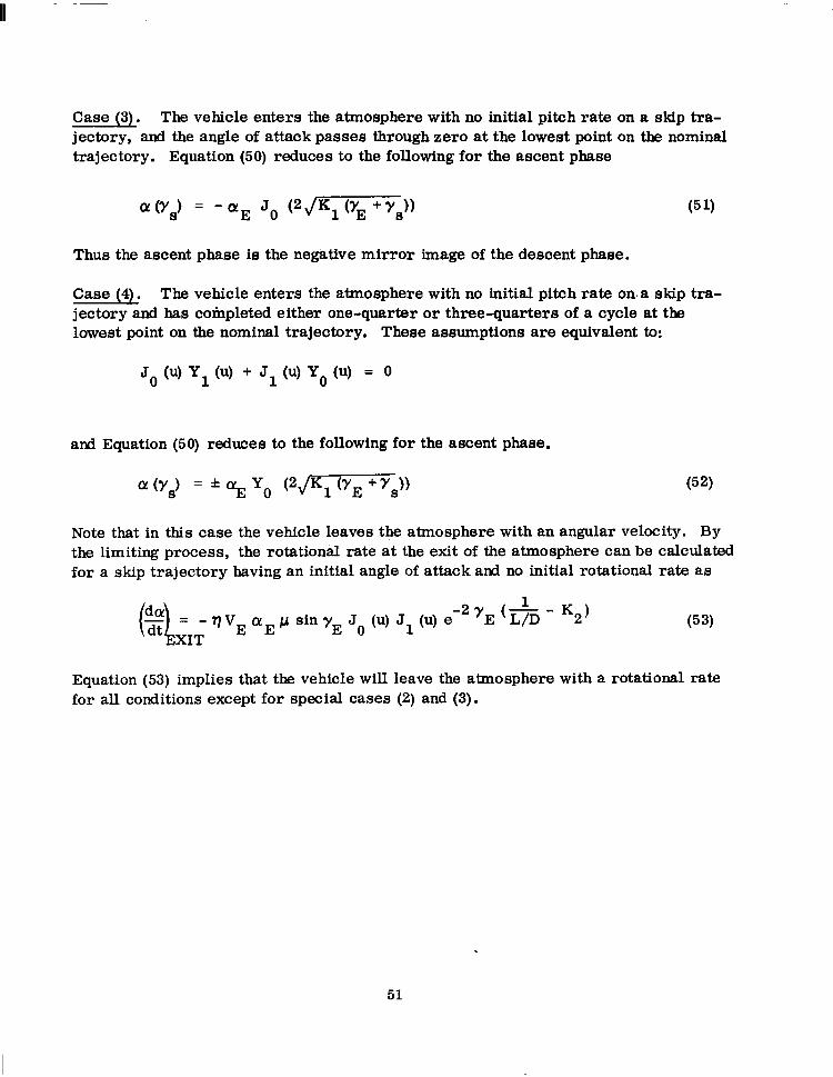
h 1 Case (3). The v e ‘c e enters the atmosphere with no initial pitch rate on a skip trajectory, and the angle of attack passes through zero at the lowest point on the nominal trajectory. Equation (50) reduces to the following for the ascent phase

a (Y,) = - aE Jo (2 ,/vsN (51)

Thus the ascent phase is the negative mirror image of the descent phase.

The vehl 1 Case (4). ‘c e enters the atmosphere with no initial pitch rate on a skip trajectory and has completed either one-quarter or three-quarters of a cycle at the lowest point on the nominal trajectory. These assumptions are equivalent to:

Jo 04 Y1 04 + J1 04 Y. 04 = 0

and Equation (50) reduces to the following for the ascent phase.

a (Y,) = * “E y. (q53pq) (52)

Note that in this case the vehicle leaves the atmosphere with an angular velocity. By the limiting process, the rotational rate at the exit of the atmosphere can be calculated for a skip trajectory having an initial angle of attack and no initial rotational rate as

- rl VE aE P sin yE Jo 0-O J1 0.9 e -2~~ (+B - X2) (53)

Equation (53) implies that the vehicle will leave the atmosphere with a rotational rate for all conditions except for special cases (2) and (3).

51

6/REFERENCES

1. Breuhaus, W; O., Reynolds, P. A., and Kidd, E. A. Handling Qualities Re- quirements for Hyper-velocity Aircraft, Cornell Aeronautical Laboratory Report No. TC-1332-F-1, January 1960.

2. Afhkenas, I. L., A Study -of Conventional Airplane Handling Qualities Require- ments, Part I, Roll Handling Qualities. AFFDL-TR-65-138 Part 1, November 1965.

3. Ashkenas, I. L., A Study of Conventional Airplane Handling Qualities Require- ments, Part II, Lateral-Directional Cscfflatory Handling Qualities. AFFDL-TR-65-138 Part II, November 1965.

4. Greer, B. Y., Stewart, J. D., Merrick, R. B., and Drinkwater, F. J. III, A Pilot Opinion Study of Lateral Control Requirements for Fighter-Type Aircraft, NASA Memo l-29-59A, March 1959.

5. Newell, F. D., Ground Simulator Evaluations of Coupled Roll-Spiral Mode Effects on Aircraft Handling Qualities, AFFDL-TR-65-39, March 1965.

6. Wingrove, R. C., Stinnett, G. W., and hmis, R. C., A Study of the Pilot’s Ability to Control an Apollo Type Vehicle During Atmosphere Entry, NASA FNxm; August 1964.

7. Eggleston, J. M., Baron, S., and Cheatham, D. C., Fixed Base SimulaUon Study of a Pilot’s Ability to Control a Winged-Satellite Vehicle During High-Drag, Variable-Lift Entries, NASA TN D-228, April 1960.

8. Taylor, L. W., Jr., Analysis of a Pilot-Airplane Lateral Instability Experienced with the X-15 Airplane, NASA TN D-1059, November 1961.

9. “Flying Qualities of Piloted Airplanesfl, MIL-F-8785 (ASG), Amendment 4, November 19 57.

10. Wingrove, R. C., A Survey of Atmosphere Re-Entry Guidance and Control Methods, IAS Paperr63-86, January 1963.

11. Wingrove, R. C., Trajectory Control Problems in the Planetary Entry of Manned Vehicles, AIAA Entry Technology Conference, October 1964.

12. Assadurian, A., and Cheatham, D. C., Longitudinal Range Control Ixlring the Atmospheric Phase of a Manned Satellite Re-entry, NASA TN D253, May 1960.

53

REFERENCES (Contd)

13. Leondes, C. T., Guidance and Control of Aerospace Vehicles, McGraw-Hill Book Company, New York, N. Y., 1963.

14. Galman, B. A., Some Fundamental Considerations for Lifting Vehicles in Return - from Satellite Orbit., Proceedings of the Fourth AFBMD/STL Symposium, Volumes 1 & 2, 1960.

15. Eggers, A. J., Alden, H. J., and Standord, E. W., A Comparative Analysis of the Performance of Long-Range Hyper-velocity Vehicles, NACA TN 4046, October 19 57.

16. Allen, H. J., and Eggers, A. J., Jr., A Study of the Motion and Aerodynamic Heating of Missiles Entering the Earth’s Atmosphere at High Supersonic Speeds, ~. -.- NACA TN 4047, October 1957.

17. Sommer, S. C., and Tobak, M., Study of the Oscillatory Motion of Manned .Vehicles Entering the Earth’s Atmosphere, NASA Memo 3-2-59A, April 1959.

18. Allen, H. J., Motion of a Ballistic Missile Angularly Misaligned with the Flight Path Upon Entering the Atmosphere and its Effect Upon Aerodynamic Heating and Mass Distance, NACA TN-4048, October 1957.

19. Tobak, M., and Allen, H. J., Analytical Investigation of the Dynamic Behavior of a Lifting Manned Re-entry Vehicle, NASA TN D-416, September 1960.

20. Noul, M. T., Schy, A. A., and Williams, J. L., Dynamic Stability and Control Problems of Piloted Re-entry from Lunar Missions, NASA TN D-986.

21. Computing Flight Control Systems for Entry Glider Lateral Control, .ASD-TDR- 62-699, February 1964.

22. Horinchi, F. Y., A Parametric Study of the Dynamic Motion of a Spinning and Non-spinning Re-entry Vehicle with Nonlinear Aerodynamic Characteristics,.. Symposium on Ballistic Missile and Aerospace Technology, 6th, 1961, Los Angeles Proceedings - V.4: Re-entry.

23. Gibson, J. E., Nonlinear Automatic Control, McGraw-Hill Book Company, New York, N. Y., 1963.

24. Frederick, H. R., and Dore, F. J., “The Dynamic Motion of a Missile Descend- ing Through the Atmosphere”,Journal of the Aeronautical Sciences, Vol. 22. 1965.

54

REFERENCES (Contd)

25. Syvertson, C. A., Swenson, B. L., Anderson, J. L., and Kenyon, G. C., “Some Considerations of the Performance of a.Maneuverable Lifting-Body Entry Vehiclelf, Advances in Astronautical Sciences, V16, Part 1, 1963.

26. Study of ElectricaIIy Produced Strain for Conlrol Purposes, AS&TDR-62-621, October 1962.

27. An Investigation of Magnetohydrodynamic Principles Applicable to Flight Control, ___-- - ASD-TDR-62-649, December 1962.

28. Kempel, R. W., The Hypersonic Lateral-Directional Dynamics of LifUng-Re- entry Vehicles, AFFTC TR-64-46, August 1965.

29. Grant, F. C., Importance of the Variation of Drag with Lift in Minimization of Satellite Entry Acceleration, NASA TN-D-1201 October 1959.

30. Etkin, B., Longitudinal Dynamics of a Lifting Vehicle in a Circular Orbit, Institute ofAerophysics, University of Toronto, AFCSR TN 60-191, February 1960.

31. Dubozanski, J. S., Re-entry Guidance and Control Using Temperature Rate Flight Control System, The Electronics Division of General Motors Corporation, August 1963.

32. Johannes, R. P., “Re-entry Energy Management”, AFFDL TR-65-61, June 1965.

33. Greensite, A. L., “Design Criteria for Control of Space VehiclesI’, Vol. 1, Part 1, Short-Period Dynamics, October 1965.

34. Webb, W. L., “The Dynamic Stratosphere”, Astronautics and Aeronautics, March 1964.

NASA-Langley, 1967 -32 CR-945 55

- -

“The aeronautical and space activities of the United States shall be conducted so as to contribute . . . to the expansion of human knowledge of phenomena in the atmosphere and space. The Administration shall provide for the widest practicable and appropriate dissemination of information concerning its activities and the reszdts thereof!’

-NATIONAL AERONALIXS AND SPACB Acr OF 1958

NASA SCIENTIFIC AND TECHNICAL PUBLICATIONS

TECHNICAL REPORTS: Scientific and technical information considered important, complete, and a lasting contribution to existing knowledge.

TECHNICAL NOTES: Information less broad in scope but nevertheIess of importance as a contribution to existing knowledge.

TECHNICAL MEMORANDUMS: Information receiving limited distribution because of preliminary data, security classification, or other reasons.

CONTRACTOR REPORTS: Scientific and technical information generated under a NASA contract or grant and considered an important contribution to existing knowledge.

TECHNICAL TRANSLATIONS: Information published in a foreign language considered to merit NASA distribution in English.

SPECIAL PUBLICATIONS: Information derived from or of value to NASA activities. Publications include conference proceedings, monographs, data compilations, handbooks, sourcebooks, and special bibliographies.

TECHNOLOGY UTILIZATION PUBLICATIONS: Information on technology used by NASA that may be of particular interest in commercial and other non-aerospace applications. Publications include Tech Briefs, Technology Utilization Reports and Notes, and Technology Surveys.

Defails on the availability of these publications may be obtained from:

SCIENTIFIC AND TECHNICAL INFORMATION DIVISION

NATIONAL AERONAUTICS AND SPACE ADMINISTRATION

Washington, D.C. PO546

DYNAMIC STABILITY OF SPACE VEHICLES

Documents

Transcript of DYNAMIC STABILITY OF SPACE VEHICLES