Stability of Three-Wheeled Vehicles with and without ... · PDF fileStability of Three-Wheeled...

International Journal of Automotive Engineering Vol. 3, Number 1, March 2013

Stability of Three-Wheeled Vehicles with and

without Control System

M. A. Saeedi 1,*

, R. Kazemi 2

1 Ph.D student, 2 Associate professor, Department of Mechanical Engineering, K. N. Toosi University of Technology,

Tehran, Iran.

*[email protected]

Abstract

In this study, stability control of a three-wheeled vehicle with two wheels on the front axle, a three-wheeled

vehicle with two wheels on the rear axle, and a standard four-wheeled vehicle are compared. For vehicle

dynamics control systems, the direct yaw moment control is considered as a suitable way of controlling the

lateral motion of a vehicle during a severe driving maneuver. In accordance to the present available

technology, the performance of vehicle dynamics control actuation systems is based on the individual

control of each wheel braking force known as the differential braking. Also, in order to design the vehicle

dynamics control system the linear optimal control theory is used. Then, to investigate the effectiveness of

the proposed linear optimal control system, computer simulations are carried out by using nonlinear twelve-

degree-of-freedom models for three-wheeled cars and a fourteen-degree-of-freedom model for a four-

wheeled car. Simulation results of lane change and J-turn maneuvers are shown with and without control

system. It is shown that for lateral stability, the three wheeled vehicle with single front wheel is more stable

than the four wheeled vehicle, which is in turn more stable than the three wheeled vehicle with single rear

wheel. Considering turning radius which is a kinematic property shows that the front single three-wheeled

car is more under steer than the other cars.

Keywords: stability, three-wheeled vehicles, differential braking, vehicle dynamics control systems.

1. Introduction

Nowadays, automobile companies are involved in

the design of more efficient vehicles improving the

energetic efficiency and making them smaller for the

best use of the current roads and streets. The idea of

smaller, energy-efficient vehicles for personal

transportation seems to naturally introduce the three

wheel platform. Opinions normally run either strongly

against or strongly in favor of the three wheel layout.

Advocates point to a mechanically simplified chassis,

lower manufacturing costs, and superior handling

characteristics. Opponents decry the three-wheeler's

propensity to overturn. Both opinions have merit.

Three-wheelers are lighter and less costly to

manufacture. But when poorly designed or in the

wrong application, a three wheel platform is the less

forgiving layout. When correctly designed, however,

a three wheel car can light new fires of enthusiasm

under tired and routine driving experiences. And

today's tilting three-wheelers, vehicles that lean into

turns like motorcycles, point the way to a new

category of personal transportation products of much

lower mass, far greater fuel economy, and superior

cornering power. Today, auto manufacturers to design

more efficient cars to improve energy and also to

make them smaller in order to better use on streets

and roads are modern. A three wheeled car, also

known as a tricar or tri-car, is an automobile having

either one wheel in the front for steering and two at

the rear for power, two in the front for steering and

one in the rear for power, or any other combination of

layouts [1,2].

Many efforts are being made in automotive

industries to develop the vehicle dynamics control

(VDC) system which improves the lateral vehicle

response in critical cornering situations by

distributing asymmetric brake forces to the wheels.

Some of the systems have already been

commercialized and are being installed in passenger

vehicles. The VDC system has a good potential of

M. A. Saeedi and R. Kazemi 344


becoming one of the chassis control necessities due to

its significant benefit at little extra cost when installed

on top of the ABS/TCS system. A critical lateral

motion of a vehicle refers to the situation when the

tire–road contactness can no longer be sustained. In

such situations, the body side slip angle grows and the

sensitivity of the yaw moment with respect to the

steer angle suddenly diminishes. An addition of the

steer angle can no longer increase the yaw moment,

which is however needed to restore the vehicle

stability. The target of the VDC system is to make the

vehicle’s lateral motion behave as commanded by the

driver’s steering action. To achieve this, the controller

generates the yaw moment to restore the stability by

distributing asymmetric brake forces to the wheels. In

vehicles without VDC, the yaw moment can be

generated only by the driver’s steering action. In

vehicles with the VDC, however, when a critical

situation is detected, the brake force becomes

exclusively under the control of the VDC and a

compensating yaw moment is generated [3].

For VDC systems, the yaw moment control is

considered as way of controlling the lateral motion of

a vehicle during a severe driving maneuver. One of

the most effective methods for improving the

handling performance and active safety of ground

vehicles in non-linear regimes is direct yaw moment

control (DYC) [4, 5].

In order to find a suitable control law for DYC, it

is necessary to have a deep understanding of vehicle

dynamics and control system limitations. From the

viewpoint of vehicle dynamics and tire

characteristics, Furukawa and Abe [6] reviewed the

several control methods proposed by previous

researchers and emphasized that, as DYC is more

effective on the vehicle motion control in a non-linear

range of vehicle dynamics and tire characteristics, the

reasonable control law should be take this

nonlinearity in to consideration. Thus, they proposed

the sliding control method for DYC and used it in

their later works [7, 8].

Some researchers have emphasized only the

development of the control logic of yaw moment

control cooperated with 4WS ignoring how the yaw

moment is generated [9, 10]. Other researchers

proposed PID controls or LQ-optimal controls to

compensate the error between the actual state and

desired state of the vehicle [11,12,13]. Also, many

studies have been done about controlling vehicle slip

ratio to generate sufficient lateral forces and

longitudinal forces [14]. However, most of them do

not guarantee the robustness to uncertainty in vehicle

parameters and disturbances that are intrinsically

associated with vehicles.

Many methods have been studied and actively

developed to improve a four-wheeled vehicle’s lateral

stability actively (Zanten et al., 1998; Nagai et al.,

1999; Nagai etal., 2002; Shino et al., 2001; Shibahata

et al., 1992, Song et al., 2007). However, there have

only been a few studies on the lateral stability of a

three-wheeled vehicle.

In the present study, comparing the stability

control of three-wheeled vehicles and a four-wheeled

one is the main goal which has never been done. In

order to do this, a linear control system for direct yaw

moment control, to improve the vehicle handling, is

developed. The control law is developed by

minimizing the difference between the predicted and

the desired yaw rate responses. The method is based

on individually controlling the braking force of each

wheel. In the case of lateral stability, it will be shown

that the three wheeled vehicle with two wheels on the

rear axle is more stable. Moreover, comparing turning

radii shows that the three-wheeled vehicle with a

single front wheel is more under steer. The optimal

control system is robust to changes, and also, has a

suitable performance while imposing changes.

Simulation results indicate that when the proposed

optimal controller is engaged with the models,

satisfactory handling performances for three kinds of

vehicles can be achieved.

This paper is organized as follows. First, two 12-

degree-of-freedom dynamic models for three-wheeled

cars and a 14-degree-of-freedom dynamic model for

four-wheeled car are used. The main reason of

adopting a 4-wheeled car in this paper is to verify the

models of 3-wheeled cars and to compare the

dynamic performance of three-wheeled cars with that

of the 4-wheeled car. Then, tire dynamics is modeled.

In order to improve the dynamic performance of

vehicles, linear optimal control theory is used, and

some design parameters for the control algorithm are

presented. Next, the validation of the four-wheeled

vehicle model, and the results of simulations in lane

change and J-turn maneuvers are presented, and the

effectiveness of the control system for three-wheeled

cars are shown. Finally, Conclusions are provided.

2. Vehicle Modeling

In this research, the vehicle dynamic model is a

nonlinear model with twelve degrees of freedom. This

model is made up of a sprung mass and four un

sprung masses. The vehicle body has six degrees of

freedom which are translational motions in x, y, and z

direction, and angular motions about those three axes.

Roll, pitch, and yaw motions are the rotation about x,

y, and z axes, respectively. Each of the wheels has

translational motion in z direction and wheel spin

345 Stability of Three-Wheeled Vehicles…..


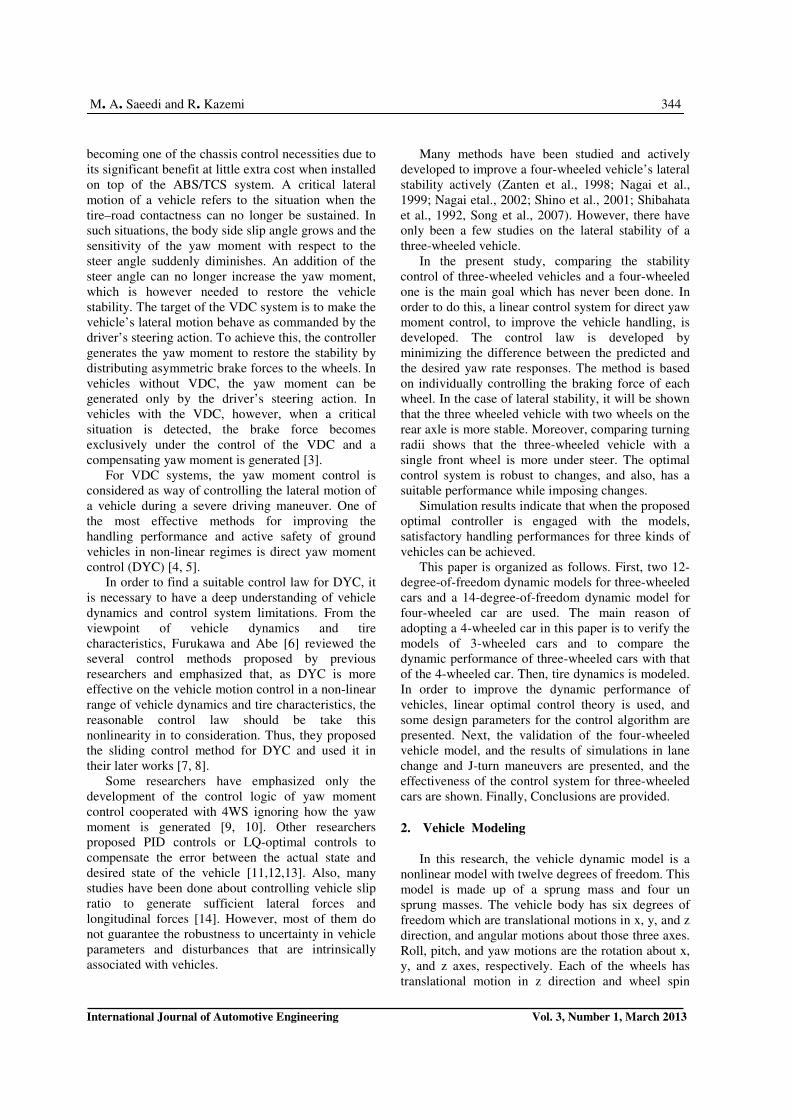
Fig1. (a) the fourteen-degree-of freedom model for four-wheeled vehicle, (b) the twelve-degree-of-freedom model for three-wheeled car

with front single wheel, (c) the twelve-degree-of-freedom model for three-wheeled car with rear single wheel

about y direction. The front wheels can steer about

the z-axis. It is worth noting that the four-wheeled

vehicle model has fourteen degrees of freedom. The

Full vehicle models are shown in Fig.1. In the

development of the vehicle model, the following

assumptions were made:

1. The steering angles � of both front wheels are

considered identical.

2. The effect of un sprung mass is ignored in the

vehicle’s pitch and roll motions.

3. The tire and suspension remain normal to the

ground during vehicle maneuvers.

4. The center of roll and pitch motion are placed

on the vehicle’s center of gravity.

2.1 Equations of motion:

Governing equations of the Longitudinal, Lateral,

and Vertical, Roll, Pitch and Yaw motions can be

expressed as [5]:

In Fig.1 (a): �� + �� − �� = �� + �� + �� +�� (1)



�� + �� − ∅� ��= �� + �� + �� + �� (2)

Where ∅� is the roll rate, and � is the pitch rate,

and � is the yaw rate. Also, �� is the tire self

aligning torque. The terms �� and �� are the

respective tire forces in the � and � directions, which

can be related to the tractive and the lateral tire forces.

F!"= Fx!" cos(δ!")− Fy!" sin(δ!") for �(i = f, r), (k= l, r)� (7)

�� = �� 123(��)+ �� 345(��) 627 �(4 = 6, 7), (8= 9, 7)� (8)

Tire Side Slip Angle:

The angle between tire directions of motion has

known as tire side slip angle and obtain based on the

following formulation.

The equations of motion for the suspension model

are as follows:

In Fig.1 (b):

Tire Side Slip Angle:

In Fig.1 (c):

�;�� + ∅� �� − �� = �<�� + �<�� + �<� (21)

�� = = >299 �2?@5A3 = B;��∅C − �B;�� − B;�� = ��<�� − �<�� D� 2⁄− �� + �� + ��ℎ (22)

�;�� + ∅� �� − ��= �<�� + �<�� + �<�� + �<�� (3)

�� = = H4A1ℎ �2?@5A3= B;��C − (B; − B;��)� �= (�<�� + �<��)9�− ��<�� + �<��9�+ �� + �� + ��+ ��)ℎ (5)

� = = �JK �2?@5A3 = B C − �B�� − B��∅� �= �� − �� D� 2⁄+ (�� − ��) 9� + ��+ ��)9� − (�� + ��)9�+ = ��

L

�MN (6)

�� = ∑ >299 �2?@5A3 = B;��∅C − �B;�� −B;)� � = ��<�� − �<�� D� 2⁄ + (�<�� −�<��) D� 2⁄ − �� + �� + �� + ��ℎ (4)

RN = AJ5SN T �� + 9� �� + D� 2⁄ �U − �� (9)

�<�� = 83N�<WX − <N� + 13N�<WX� − <N� � �<�� = 83Y�<WZ − <Y� + 13Y�<WZ� − <Y� � �<�� = 83[�<W\ − <[� + 13[�<W\� − <[� �

�<�� = 83L�<W] − <L� + 13L�<W]� − <L� � (10) And <�� = <a − �D� 2⁄ b� − 9� <�� = <a + �D� 2⁄ b� − 9� <�� = <a − (D� 2⁄ b) + 9� <�� = <a + (D� 2⁄ b) + 9� (11)

�� + �� − �� = �� + �� + �� (12) �� + �� − ∅� �� = �� + �� + �� (13) �;�� + ∅� �� − �� = �<� + �<�� + �<�� (14)

�� = = H4A1ℎ �2?@5A3= B;��C − (B; − B;��)� �= (�<�� + �<��)9� − ��<�9��+ �� + �� + ��ℎ (16)

� = = �JK �2?@5A3 = B C − �B�� − B��∅� �= (�� − ��) D� 2⁄ − (�� + ��)9� + ��9��+ = ��

[

�MN (17)

�� = ∑ >299 �2?@5A3 = B;��∅C − �B;�� −B;)� � = (�<�� − �<��) (15)

RN = AJ5SN T�� + 9� �� U − ��

RY = AJ5SN T �� − 9� �� + D� 2⁄ � U

R[ = AJ5SN c deS�fg�dhSif Y⁄ g� j (18)

�� + �� − �� = �� + �� + �� (19) �� + �� − ∅� �� = �� + �� + �� (20)

347 Stability of Three-Wheeled Vehicles…..


Tire Side Slip Angle

2.2 Tire Dynamics

Apart from aerodynamic forces, all of the forces

influencing the vehicle are created on the contact

surface between the tire and the road. Hence, in the

vehicle dynamic behavior simulation, the nonlinear

behavior of a tire is considered the most effective

factor. In this model, the combined slip situation was

modeled from a physical viewpoint. Tires generate

lateral and longitudinal forces in a non-linear manner.

In this paper, the combined slip Magic Formula of the

tire model (1993) is used since it can provide

considerable qualitative agreement between theory

and the measured data. This model describes the

effect of combined slip on the lateral force and on the

longitudinal force characteristics. The general

mathematical formulation of the Magic Formula

model is presented in the Appendix, and reference

[15].

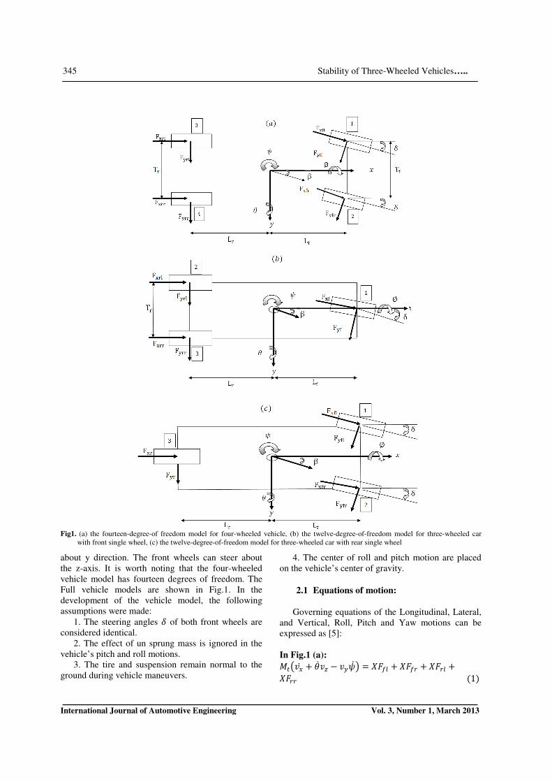
2.3 Wheel Dynamics

The following equation can be written for traction,

from Figure 2:

Note that in braking

where k� and �� denote rotational speed and

longitudinal force associated with wheel 4, Bl is the

spin inertia of the wheel, 7l is the tire rolling radius

and D is the input drive or brake torque coming to the

wheel [16].

Fig2. wheel rotation [7]

�� = = H4A1ℎ �2?@5A3= B;��C − (B; − B;��)� �= �<�9� − ��<�� + �<��9�+ �� + �� + ��ℎ (23)

� = = �JK �2?@5A3 = B C − �B�� − B��∅� �= �� − �� D� 2⁄ + �� + ��9� − (��9�)+ = ��

[

�MN (24)

RN = AJ5SN T �� + 9� �� + D� 2⁄ �U − ��

RY = AJ5SN T �� + 9� �� − D� 2⁄ �U − ��

R[ = AJ5SN T�� − 9� �� U (25)

km� = 1Bl

(D − 7l��) (26)

km� = 1Bl

(−D + 7l��) (27)



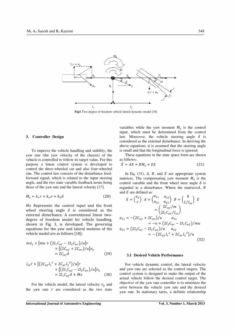
Fig3. Two-degree of freedom vehicle lateral dynamic model [18]

3. Controller Design

To improve the vehicle handling and stability, the

yaw rate (the yaw velocity of the chassis) of the

vehicle is controlled to follow its target value. For this

purpose a linear control system is developed to

control the three-wheeled car and also four-wheeled

one. The control law consists of the disturbance feed-

forward signal, which is related to the input steering

angle, and the two state variable feedback terms being

those of the yaw rate and the lateral velocity [17].

�n = 8�7 + 8d� + 8o� (28)

For the vehicle model, the lateral velocity �� and

the yaw rate 7 are considered as the two state

variables while the yaw moment � is the control

input, which must be determined from the control

law. Moreover, the vehicle steering angle � is

considered as the external disturbance. In deriving the

above equations, it is assumed that the steering angle

is small and that the longitudinal force is ignored.

These equations in the state space form are shown

as follows: �� = p� + q� + r� (31)

In Eq. (31), p, q, and r are appropriate system

matrices. The compensating yaw moment � is the

control variable and the front wheel steer angle � is

regarded as a disturbance. Where the matricesp, q

and r are defined as:

3.1 Desired Vehicle Performance

For vehicle dynamic control, the lateral velocity

and yaw rate are selected as the control targets. The

control system is designed to make the output of the

actual vehicle follow the desired control target. The

objective of the yaw rate controller is to minimize the

error between the vehicle yaw rate and the desired

yaw rate. In stationary turns, a definite relationship

?�� + s?t + �29Nuv� − 29Yuv�� t⁄ w7+ s�2uv� + 2uv�� t⁄ w��= 2uv�� (29)

B7� + s�2uv�9NY + 2uv�9YY� t⁄ w7+ s�29Nuv� − 29Yuv�� t⁄ w��= 29Nuv�� + �< (30)

�< Represents the control input and the front wheel steering angle � is considered as the external disturbance. A conventional linear two-degree of freedom model for vehicle handling, shown in Fig. 3, is developed. The governing equations for the yaw and lateral motions of the vehicle model are as follows [18]:

� = c��7 j p = �JNN JNYJYN JYY � q = � 01 B⁄ � r

= T 2uv� ?⁄29Nuv� B⁄ U

JNN = −�2uv� + 2uv�� t⁄ JNY= −t + �29Yuv� − 29Nuv�� ?t⁄ JYN = �29Yuv� − 29Nuv�� t⁄ JYY= − �2uv�9NY + 2uv�9YY� t⁄ (32)

349 Stability of Three-Wheeled Vehicles….


exists between the steering angle, the vehicle

longitudinal velocity, and the yaw rate. This

relationship is used to drive the desired yaw rate [19]:

Where 8W; is usually referred to as the under steer

coefficient.

It is important to note that the control effort �<

must satisfy some physical constrains due to both the

actuation system and the road-tire performance limits.

To satisfy those limits, the control effort �< in the

performance index must be written as in the following

form [17].

To determine the values of the feedback and feed-

forward control gains, which are based on the defined

performance index and the vehicle dynamic model, a

LQR problem has been formulated for which its

analytical solution is obtained, [20].

In that case, the performance index of Eq. (34)

may be rewritten in the following form

Where

The Hamiltonian function, in the expanded form,

is given by:

Where �� is the desired reference value of the

state vector, � is a real symmetric positive semi-

definite matrix, and > is a real symmetric positive

definite matrix, and

H = c�N�Yj (38)

Where the parameters �N and �Y are the

Lagrangian multipliers.

The cost ate equations are

and the algebraic relations that must be satisfied

are given by �� = >� + qiH = 0 (40)

Therefore,

Considering that the current optimal control

problem is a Tracking type, the matrix H is as

following H = �� + � (43)

Next, by substituting eq. (43) into (42), we will

have

Differentiating both sides with respect to A, we

obtain

Substituting from eq. (39) for H� and eq. (41) for �� , and using eq. (43) to eliminate H, the following

relations can be obtained:

By assuming that the solutions of the equations

converge rapidly to the constant values, therefore �� = 0 and �� = 0

Using the above assumptions, the following

system of algebraic equations could then be formed: pi� + �p + � − �q>SNqi� = 0 (48) (pi + �q>SNqi)� − �� + r� = 0 (49)

By solving equations (48) and (49) for � and �,

the control input can be fully calculated.

4. Simulation Results With The Vehicle Control

System

Validation of Four-Wheel Vehicle Model

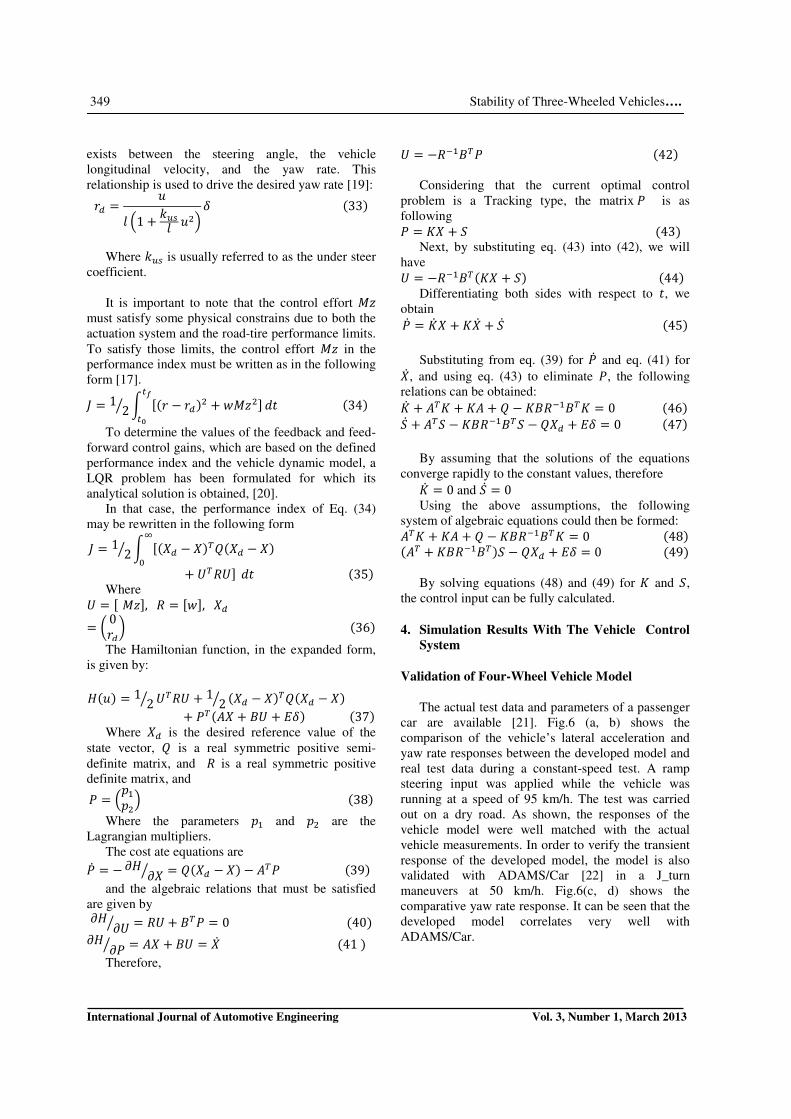
The actual test data and parameters of a passenger

car are available [21]. Fig.6 (a, b) shows the

comparison of the vehicle’s lateral acceleration and

yaw rate responses between the developed model and

real test data during a constant-speed test. A ramp

steering input was applied while the vehicle was

running at a speed of 95 km/h. The test was carried

out on a dry road. As shown, the responses of the

vehicle model were well matched with the actual

vehicle measurements. In order to verify the transient

response of the developed model, the model is also

validated with ADAMS/Car [22] in a J_turn

maneuvers at 50 km/h. Fig.6(c, d) shows the

comparative yaw rate response. It can be seen that the

developed model correlates very well with

ADAMS/Car.

7� = t9 c1 + 8W;9 tYj � (33)

� = 1 2� � [(7 − 7�)Y + K�<Y]��

�A (34)

� = 1 2� � [(�� − �)i�(�� − �)�� + �i>�] �A (35)

� = [ �<], > = [K], ��= � 07�� (36)

�(t) = 1 2� �i>� + 1 2� (�� − �)i�(�� − �)+ Hi(p� + q� + r�) (37)

H� = − �� = �(�� − �) − piH (39)

�� H� = p� + q� = �� (41 )

� = −>SNqiH (42)

� = −>SNqi(�� + �) (44)

H� = �� + �� + �� (45)

�� + pi� + �p + � − �q>SNqi� = 0 (46) �� + pi� − �q>SNqi� − �� + r� = 0 (47)



Fig4. Model validation results. with real test data: (a) Lateral acceleration. (b) Yaw rate response. With ADAMS/CAR: (c) Wheel steer angle.

(d) Yaw rate response.

To study the transient performance of the

proposed controller, numerical simulations are carried

out with the aim of simulation software based on

MATLAB and M-File for vehicles dynamic behavior

during lane change and J-turn maneuvers between the

cases with and without control. The effectiveness of

the controller is shown considering two different

steering angle inputs:

(a) a single lane change maneuver completed in

2s with two triangular pulses �� = ±3��.

(b) a J-turn maneuver produced from the ramp

steer input �� = +3��.

It should be noted that all of the vehicle

parameters are the same, and only in the cases of

single wheel 8� and 1� coefficients are doubled.

4.1 Vehicle dynamics under a single lane

change maneuver

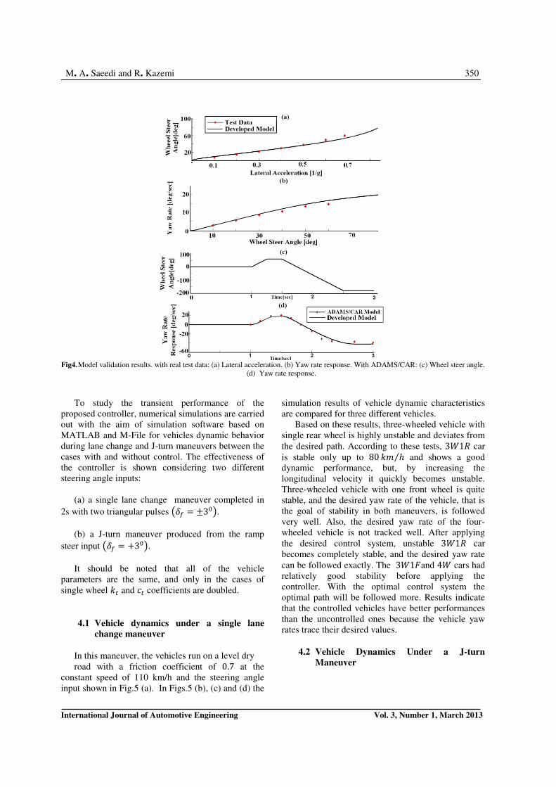
In this maneuver, the vehicles run on a level dry

road with a friction coefficient of 0.7 at the

constant speed of 110 km/h and the steering angle

input shown in Fig.5 (a). In Figs.5 (b), (c) and (d) the

simulation results of vehicle dynamic characteristics

are compared for three different vehicles.

Based on these results, three-wheeled vehicle with

single rear wheel is highly unstable and deviates from

the desired path. According to these tests, 3�1> car

is stable only up to 80 8? ℎ⁄ and shows a good

dynamic performance, but, by increasing the

longitudinal velocity it quickly becomes unstable.

Three-wheeled vehicle with one front wheel is quite

stable, and the desired yaw rate of the vehicle, that is

the goal of stability in both maneuvers, is followed

very well. Also, the desired yaw rate of the four-

wheeled vehicle is not tracked well. After applying

the desired control system, unstable 3�1> car

becomes completely stable, and the desired yaw rate

can be followed exactly. The 3�1�and 4� cars had

relatively good stability before applying the

controller. With the optimal control system the

optimal path will be followed more. Results indicate

that the controlled vehicles have better performances

than the uncontrolled ones because the vehicle yaw

rates trace their desired values.

4.2 Vehicle Dynamics Under a J-turn

Maneuver



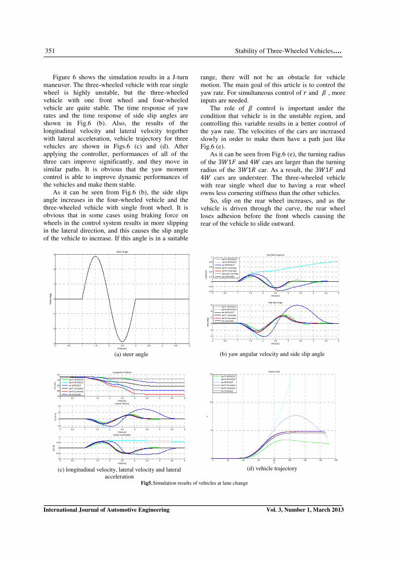
Figure 6 shows the simulation results in a J-turn

maneuver. The three-wheeled vehicle with rear single

wheel is highly unstable, but the three-wheeled

vehicle with one front wheel and four-wheeled

vehicle are quite stable. The time response of yaw

rates and the time response of side slip angles are

shown in Fig.6 (b). Also, the results of the

longitudinal velocity and lateral velocity together

with lateral acceleration, vehicle trajectory for three

vehicles are shown in Figs.6 (c) and (d). After

applying the controller, performances of all of the

three cars improve significantly, and they move in

similar paths. It is obvious that the yaw moment

control is able to improve dynamic performances of

the vehicles and make them stable.

As it can be seen from Fig.6 (b), the side slips

angle increases in the four-wheeled vehicle and the

three-wheeled vehicle with single front wheel. It is

obvious that in some cases using braking force on

wheels in the control system results in more slipping

in the lateral direction, and this causes the slip angle

of the vehicle to increase. If this angle is in a suitable

range, there will not be an obstacle for vehicle

motion. The main goal of this article is to control the

yaw rate. For simultaneous control of 7 and � , more

inputs are needed.

The role of � control is important under the

condition that vehicle is in the unstable region, and

controlling this variable results in a better control of

the yaw rate. The velocities of the cars are increased

slowly in order to make them have a path just like

Fig.6 (e).

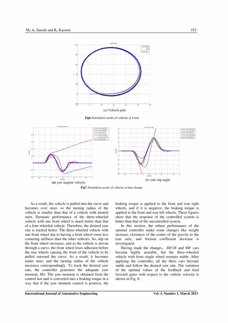
As it can be seen from Fig.6 (e), the turning radius

of the 3�1� and 4� cars are larger than the turning

radius of the 3�1> car. As a result, the 3�1� and 4� cars are understeer. The three-wheeled vehicle

with rear single wheel due to having a rear wheel

owns less cornering stiffness than the other vehicles.

So, slip on the rear wheel increases, and as the

vehicle is driven through the curve, the rear wheel

loses adhesion before the front wheels causing the

rear of the vehicle to slide outward.

(a) steer angle

(b) yaw angular velocity and side slip angle

(c) longitudinal velocity, lateral velocity and lateral

acceleration

(d) vehicle trajectory

Fig5. Simulation results of vehicles at lane change

0 0.5 1 1.5 2 2.5 3 3.5 4 4.5 5-3

-2

-1

0

1

2

3Steer Angle

time[sec]

Deltaf

[deg] 0 0.5 1 1.5 2 2.5 3 3.5 4 4.5 5

-0.4

-0.2

0

0.2

0.4

0.6

0.8

1Yaw Rate response

time[sec]

r [r

ad/s

ec]

0 0.5 1 1.5 2 2.5 3 3.5 4 4.5 5

-4

-2

0

2

4

6Side Slip Angle

time[sec]

beta

[deg]

3w1F WITHOUT

3w1R WITHOUT

4w WITHOUT

3w1F Controled

3w1R Controled

Desired Yaw Rate

4w Controled

3w1F WITHOUT

3w1R WITHOUT

4w WITHOUT

3w1F Controled

3w1R Controled

4w Controled

0 0.5 1 1.5 2 2.5 3 3.5 4 4.5 527

28

29

30

31Longitudinal Velocity

time[sec]

Vx [

m/s

]

0 0.5 1 1.5 2 2.5 3 3.5 4 4.5 5

-2

0

2

4Lateral Velocity

time[sec]

Vy [

m/s

]

0 0.5 1 1.5 2 2.5 3 3.5 4 4.5 5-1

-0.5

0

0.5

1Lateral acceleration

time[sec]

ay[1

/g]

3w1F WITHOUT

3w1R WITHOUT

4w WITHOUT

3w1F Controled

3w1R Controled

4w Controled

0 20 40 60 80 100 120 140 1600

5

10

15Vehicle Path

X

Y

3w1F WITHOUT

3w1R WITHOUT

4w WITHOUT

3w1F Controled

3w1R Controled

4w Controled



(e) Vehicle path

Fig6. Simulation results of vehicles at J-turn

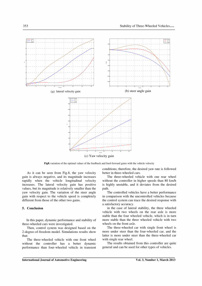
Fig7. Simulation results of vehicles at lane change.

As a result, the vehicle is pulled into the curve and

becomes over steer, so the turning radius of the

vehicle is smaller than that of a vehicle with neutral

steer. Dynamic performance of the three-wheeled

vehicle with one front wheel is much better than that

of a four-wheeled vehicle. Therefore, the desired yaw

rate is tracked better. The three-wheeled vehicle with

one front wheel due to having a front wheel owns less

cornering stiffness than the other vehicles. So, slip on

the front wheel increases, and as the vehicle is driven

through a curve, the front wheel loses adhesion before

the rear wheels causing the front of the vehicle to be

pulled outward the curve. As a result, it becomes

under steer, and the turning radius of the vehicle

increases correspondingly. To track the desired yaw

rate, the controller generates the adequate yaw

moment, �<. The yaw moment is obtained from the

control law and is converted into a braking torque in a

way that if the yaw moment control is positive, the

braking torque is applied to the front and rear right

wheels, and if it is negative, the braking torque is

applied to the front and rear left wheels. These figures

show that the response of the controlled system is

better than that of the uncontrolled system.

In this section, the robust performance of the

optimal controller under some changes like weight

increase, closeness of the center of the gravity to the

rear axle, and friction coefficient decrease is

investigated.

Having made the changes, 3�1> and 4� cars

become highly unstable, but the three-wheeled

vehicle with front single wheel remains stable. After

applying the controller, all the three cars become

stable and follow the desired yaw rate. The variation

of the optimal values of the feedback and feed

forward gains with respect to the vehicle velocity is

shown in Fig. 8.

-20 0 20 40 60 80 100-20

0

20

40

60

80

100Vehicle Path

X

Y

3w1F

3w1R

4w

(a) yaw angular velocity (b) side slip angle

0 0.5 1 1.5 2 2.5 3 3.5 4 4.5 5-0.4

-0.2

0

0.2

0.4

0.6

0.8

1Yaw Rate response

time[sec]

r [r

ad/s

ec]

3w1F WITHOUT

3w1R WITHOUT

4w WITHOUT

3w1F Controled

3w1R Controled

Desired Yaw Rate

4w Controled

0 0.5 1 1.5 2 2.5 3 3.5 4 4.5 5-5

-4

-3

-2

-1

0

1

2

3

4

5Side Slip Angle

time[sec]

beta

[deg]

3w1F WITHOUT

3w1R WITHOUT

4w WITHOUT

3w1F Controled

3w1R Controled

4w Controled



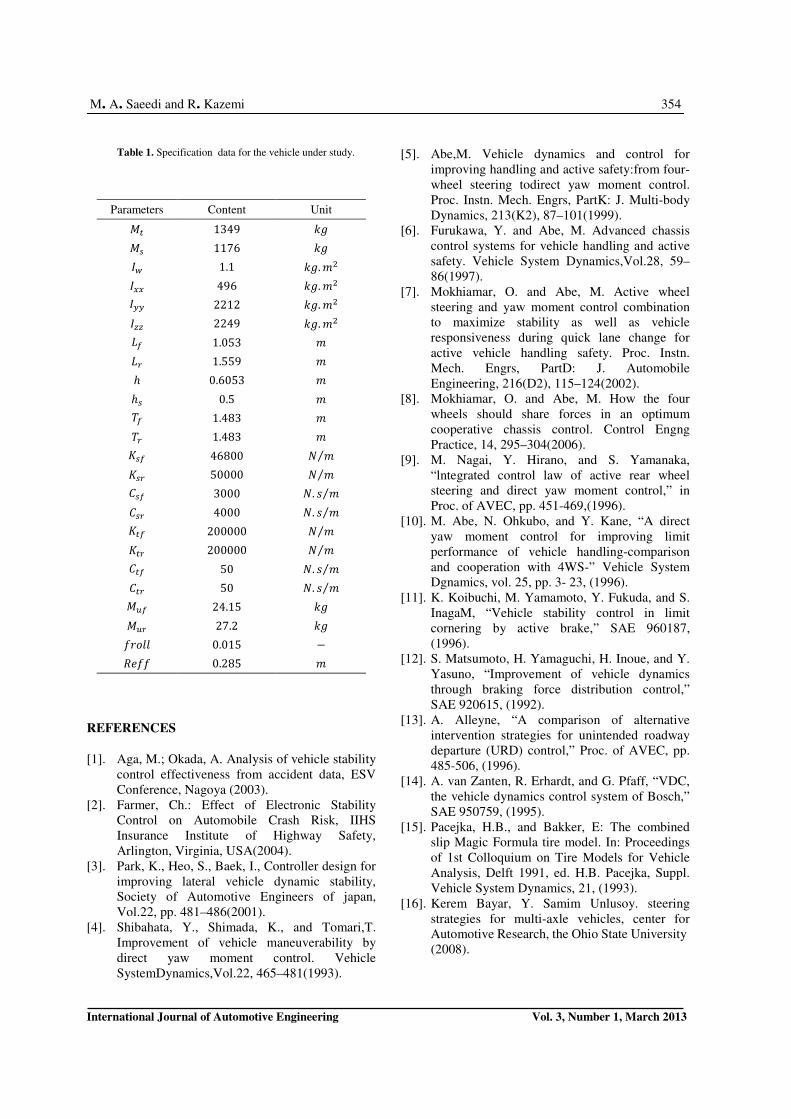
(c) Yaw velocity gain

Fig8. variation of the optimal values of the feedback and feed-forward gains with the vehicle velocity

As it can be seen from Fig.8, the yaw velocity

gain is always negative, and its magnitude increases

rapidly when the vehicle longitudinal velocity

increases. The lateral velocity gain has positive

values, but its magnitude is relatively smaller than the

yaw velocity gain. The variation of the steer angle

gain with respect to the vehicle speed is completely

different from those of the other two gains.

5. Conclusion

In this paper, dynamic performance and stability of

three-wheeled cars were investigated.

Then, control system was designed based on the

2-degree-of-freedom model. Simulations results show

that:

The three-wheeled vehicle with one front wheel

without the controller has a better dynamic

performance than four-wheeled vehicle in transient

conditions; therefore, the desired yaw rate is followed

better in three-wheeled cars.

The three-wheeled vehicle with one rear wheel

without the controller in higher speeds than 80 km/h

is highly unstable, and it deviates from the desired

path.

The controlled vehicles have a better performance

in comparison with the uncontrolled vehicles because

the control system can trace the desired response with

a satisfactory accuracy.

in the case of lateral stability, the three wheeled

vehicle with two wheels on the rear axle is more

stable than the four wheeled vehicle, which is in turn

more stable than the three wheeled vehicle with two

wheels on the front axle.

The three-wheeled car with single front wheel is

more under steer than the four-wheeled car, and the

latter is more under steer than the three-wheeled car

with single rear wheel.

The results obtained from this controller are quite

general and can be used for other types of vehicles.

0 5 10 15 20 25 30 35

0

200

400

600

800

1000

1200

1400

1600

1800

Vx(m/s)

-kr

3w1F

4w

3w1R

(a) lateral velocity gain

(b) steer angle gain

0 5 10 15 20 25 30 35

0

1

2

3

4

5

6

7

Vx(m/s)

kv

3w1F

4w

3w1R

0 5 10 15 20 25 30 35

-12000

-10000

-8000

-6000

-4000

-2000

0

2000

Vx(m/s)

k d

elt

a

3w1F

4w

3w1R



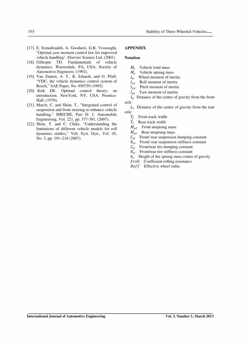
Table 1. Specification data for the vehicle under study.

Unit Content Parameters

8 1349 ��

8 1176 �;

8 . ?Y 1.1 Bl

8 . ?Y 496 B��

8 . ?Y 2212 B��

8 . ?Y 2249 B

? 1.053 ¡� ? 1.559 ¡� ? 0.6053 ℎ ? 0.5 ℎ; ? 1.483 D� ? 1.483 D�

¢ ?⁄ 46800 �;� ¢ ?⁄ 50000 �;�

¢. 3 ?⁄ 3000 u;� ¢. 3 ?⁄ 4000 u;� ¢ ?⁄ 200000 �� ¢ ?⁄ 200000 ��

¢. 3 ?⁄ 50 u�� ¢. 3 ?⁄ 50 u��

8 24.15 �W� 8 27.2 �W� − 0.015 67299 ? 0.285 >@66

REFERENCES

[1]. Aga, M.; Okada, A. Analysis of vehicle stability

control effectiveness from accident data, ESV

Conference, Nagoya (2003).

[2]. Farmer, Ch.: Effect of Electronic Stability

Control on Automobile Crash Risk, IIHS

Insurance Institute of Highway Safety,

Arlington, Virginia, USA(2004).

[3]. Park, K., Heo, S., Baek, I., Controller design for

improving lateral vehicle dynamic stability,

Society of Automotive Engineers of japan,

Vol.22, pp. 481–486(2001).

[4]. Shibahata, Y., Shimada, K., and Tomari,T.

Improvement of vehicle maneuverability by

direct yaw moment control. Vehicle

SystemDynamics,Vol.22, 465–481(1993).

[5]. Abe,M. Vehicle dynamics and control for

improving handling and active safety:from four-

wheel steering todirect yaw moment control.

Proc. Instn. Mech. Engrs, PartK: J. Multi-body

Dynamics, 213(K2), 87–101(1999).

[6]. Furukawa, Y. and Abe, M. Advanced chassis

control systems for vehicle handling and active

safety. Vehicle System Dynamics,Vol.28, 59–

86(1997).

[7]. Mokhiamar, O. and Abe, M. Active wheel

steering and yaw moment control combination

to maximize stability as well as vehicle

responsiveness during quick lane change for

active vehicle handling safety. Proc. Instn.

Mech. Engrs, PartD: J. Automobile

Engineering, 216(D2), 115–124(2002).

[8]. Mokhiamar, O. and Abe, M. How the four

wheels should share forces in an optimum

cooperative chassis control. Control Engng

Practice, 14, 295–304(2006).

[9]. M. Nagai, Y. Hirano, and S. Yamanaka,

“lntegrated control law of active rear wheel

steering and direct yaw moment control,” in

Proc. of AVEC, pp. 451-469,(1996).

[10]. M. Abe, N. Ohkubo, and Y. Kane, “A direct

yaw moment control for improving limit

performance of vehicle handling-comparison

and cooperation with 4WS-” Vehicle System

Dgnamics, vol. 25, pp. 3- 23, (1996).

[11]. K. Koibuchi, M. Yamamoto, Y. Fukuda, and S.

InagaM, “Vehicle stability control in limit

cornering by active brake,” SAE 960187,

(1996).

[12]. S. Matsumoto, H. Yamaguchi, H. Inoue, and Y.

Yasuno, “Improvement of vehicle dynamics

through braking force distribution control,”

SAE 920615, (1992).

[13]. A. Alleyne, “A comparison of alternative

intervention strategies for unintended roadway

departure (URD) control,” Proc. of AVEC, pp.

485-506, (1996).

[14]. A. van Zanten, R. Erhardt, and G. Pfaff, “VDC,

the vehicle dynamics control system of Bosch,”

SAE 950759, (1995).

[15]. Pacejka, H.B., and Bakker, E: The combined

slip Magic Formula tire model. In: Proceedings

of 1st Colloquium on Tire Models for Vehicle

Analysis, Delft 1991, ed. H.B. Pacejka, Suppl.

Vehicle System Dynamics, 21, (1993).

[16]. Kerem Bayar, Y. Samim Unlusoy. steering

strategies for multi-axle vehicles, center for

Automotive Research, the Ohio State University

(2008).



[17]. E. Esmailzadeh, A. Goodarzi, G.R. Vossoughi,

"Optimal yaw moment control law for improved

vehicle handling", Elsevier Science Ltd, (2001).

[18]. Gillespie TD. Fundamentals of vehicle

dynamics. Warrendale, PA, USA: Society of

Automotive Engineers; (1992).

[19]. Van Zanten, A. T., K. Erhardt, and G. Pfaff,

“VDC, the vehicle dynamics control system of

Bosch,” SAE Paper, No. 950759 (1995).

[20]. Kirk DE. Optimal control theory; an

introduction. NewYork, NY, USA: Prentice-

Hall; (1970).

[21]. March, C. and Shim, T., "Integrated control of

suspension and front steering to enhance vehicle

handling," IMECHE, Part D: J. Automobile

Engineering, Vol. 221, pp. 377-391, (2007).

[22]. Shim, T. and C. Chike, “Understanding the

limitations of different vehicle models for roll

dynamics studies,” Veh. Syst. Dyn., Vol. 45,

No. 3, pp. 191–216 (2007).

APPENDIX

Notation

�� Vehicle total mass �; Vehicle sprung mass Bl Wheel moment of inertia B�� Roll moment of inertia B�� Pitch moment of inertia

B Yaw moment of inertia ¡� Distance of the center of gravity from the front

axle ¡� Distance of the center of gravity from the rear

axle D� Front track width

D� Rear track width �W� Front unsprung mass

�W� Rear unsprung mass u;� Front/ rear suspension damping constant �;� Front/ rear suspension stiffness constant u�� Front/rear tire damping constant �� Front/rear tire stiffness constant ℎ; Height of the sprung mass center of gravity 67299 Coefficient rolling resistance >@66 Effective wheel radiu

Stability of Three-Wheeled Vehicles with and without ... · PDF fileStability of Three-Wheeled...

Documents

Transcript of Stability of Three-Wheeled Vehicles with and without ... · PDF fileStability of Three-Wheeled...