Taxonomies moléculaire et morphologique chez les foraminifères ...
245
HAL Id: tel-01048643 https://tel.archives-ouvertes.fr/tel-01048643 Submitted on 25 Jul 2014 HAL is a multi-disciplinary open access archive for the deposit and dissemination of sci- entific research documents, whether they are pub- lished or not. The documents may come from teaching and research institutions in France or abroad, or from public or private research centers. L’archive ouverte pluridisciplinaire HAL, est destinée au dépôt et à la diffusion de documents scientifiques de niveau recherche, publiés ou non, émanant des établissements d’enseignement et de recherche français ou étrangers, des laboratoires publics ou privés. Taxonomies moléculaire et morphologique chez les foraminifères planctoniques : élaboration d’un référentiel et cas particuliers de Globigerinoides sacculifer et Neogloboquadrina pachyderma Aurore André To cite this version: Aurore André. Taxonomies moléculaire et morphologique chez les foraminifères planctoniques: élab- oration d’un référentiel et cas particuliers de Globigerinoides sacculifer et Neogloboquadrina pachy- derma. Paléontologie. Université Claude Bernard - Lyon I, 2013. Français. <NNT: 2013LYO10200>. <tel-01048643>
Transcript of Taxonomies moléculaire et morphologique chez les foraminifères ...
HAL Id: tel-01048643https://tel.archives-ouvertes.fr/tel-01048643
Submitted on 25 Jul 2014
HAL is a multi-disciplinary open accessarchive for the deposit and dissemination of sci-entific research documents, whether they are pub-lished or not. The documents may come fromteaching and research institutions in France orabroad, or from public or private research centers.
L’archive ouverte pluridisciplinaire HAL, estdestinée au dépôt et à la diffusion de documentsscientifiques de niveau recherche, publiés ou non,émanant des établissements d’enseignement et derecherche français ou étrangers, des laboratoirespublics ou privés.
Taxonomies moléculaire et morphologique chez lesforaminifères planctoniques : élaboration d’un référentiel
et cas particuliers de Globigerinoides sacculifer etNeogloboquadrina pachyderma
Aurore André
To cite this version:Aurore André. Taxonomies moléculaire et morphologique chez les foraminifères planctoniques : élab-oration d’un référentiel et cas particuliers de Globigerinoides sacculifer et Neogloboquadrina pachy-derma. Paléontologie. Université Claude Bernard - Lyon I, 2013. Français. <NNT : 2013LYO10200>.<tel-01048643>

N° d’ordre 200-2013 Année 2013
THESE DE L’UNIVERSITE DE LYON
Délivrée par
L’UNIVERSITE CLAUDE BERNARD LYON 1
ECOLE DOCTORALE E2M2
DIPLOME DE DOCTORAT
(arrêté du 7 août 2006)
soutenue publiquement le 14 Novembre 2013
par
Madame Aurore ANDRE
Taxonomies moléculaire et morphologique chez les foraminifères
planctoniques : élaboration d'un référentiel et cas particuliers de
Globigerinoides sacculifer et Neogloboquadrina pachyderma
Directeurs
Gilles ESCARGUEL, Frédéric QUILLEVERE, Thibault de GARIDEL-THORON
JURY :
M. J. Dolan DR. CNRS Observatoire Océanologique de Villefranche/mer
M. R. Schiebel Pr. Université d’Angers
M. C. Douady Pr. Université Lyon 1
M. C. de Vargas DR. CNRS Station biologique de Roscoff
M. T. de Garidel –Thoron CR. CNRS CEREGE, Université Aix-Marseille
M. G. Escarguel MCF Université Lyon 1
M. F. Quillévéré MCF Université Lyon 1


_____________________________________________________________________Remerciements
2
Remerciements
Je tiens tout d’abord à remercier mes directeurs de thèse, Frédéric Quillévéré, Gilles
Escarguel et Thibault de Garidel-Thoron de m’avoir encadrée sur ce sujet aux frontières de la
biologie et de la géologie. Je les remercie également pour leur disponibilité et leur patience
sans faille.
Je remercie Christophe Douady qui a supervisé les analyses moléculaires et m’a permis de
hanter le LEHNA pendant une bonne partie de ces trois dernières années.
Je remercie Elisabeth Michel qui a collecté le matériel lors de la campagne OISO 21 et
Colomban de Vargas qui a également fourni du matériel biologique.
Je remercie Ralf Schiebel d’avoir accepté de rapporter cette thèse et pour son accueil au sein
du Laboratoire des Bio-Indicateurs Actuels et Fossiles d’Angers. Je remercie également John
Dolan qui a accepté d’être rapporteur dans un délai aussi bref.
Je voudrais remercier pour leur aide :
Raphael Morard qui m’a appris les bases de l’analyse de l’ADN chez les foraminifères et la
manipulation d’Adobe Illustrator. Je le remercie également pour son aide graphique et pour
ses nombreuses discussions.
Lara Konecny et Marie-Rose Viricel pour les manips de biologie moléculaire, pour le bon
fonctionnement du laboratoire tout au long de ces années de thèse et pour m’avoir gentiment
accueillie dans leur bureau.
Michal Kucera, Ralph Aurahs et Agnes Weiner pour avoir partagé avec moi leur méthode de
récolte ce qui a permis de donner un grand coup d’accélérateur à cette thèse. Je les remercie
également de m’avoir accueilli à Tübingen en Juillet 2011.
Tristan Lefébure qui m’a montré comment utiliser le serveur Proasellus sans lequel le calcul
de certains arbres ne serait toujours pas achevé.
Gilles Escarguel pour son aide et ses réponses rapides et claires sur les questions de
statistique.
Noëlle Buchet et Yurika Ujiié qui m’ont initié à la collecte et au tri des foraminifères
planctoniques. Je remercie Noëlle de m’avoir soutenu le moral durant la campagne Kh10-4.
_____________________________________________________________________Remerciements
3
Elisabeth Michel, Marie-Hélène Castéra, Linda Rossignol, Gulay Isguder et Julie Meilland
pour leur aide lors de la campagne OISO 19.
Yves Gally pour avoir hébergé des foraminifères dans son congélateur à La Réunion.
Je remercie également mes amis doctorants. Alexandra que je connais depuis la L3, avec qui
j’ai partagé rapports de terrain, appartements, cours de suédois, semestre Erasmus, préparation
à l’agrégation, répétitions de théâtre, grandes discussions pas toujours très sérieuses, un
nombre incalculable de repas…bref, une amie formidable. Je remercie aussi le reste de la
bande, Delphine, Abel, Emmanuel et Kévin, qui ont rendu ces années de thèse bien agréables.
Je n’oublie pas Gatsby et Elsa qui ont successivement partagé mon bureau.
Je voudrais également remercier mes amis chevaux : Fascinating, Thélème et Nataelle, et
toute l’équipe des cavaliers: Florence, Jean-Marc, Marc, Marie, Martin, Morgane, Olivia,
Olivier, Stéphane, Véronique, Virginie, et notre moniteur, Gérard. Grace à vous, la semaine
ne peut que bien se terminer.
Je n’oublie pas mes professeurs de SVT, Thierry Decaux (6ième
5ième
3ième
), Agnès Ménéroud
(2nd
1ière
TS) et Olivier Monnier dit « Momo » (Math sup), qui m’ont fait aimer la géologie et
la biologie.
Enfin je remercie ma grand’mère Mireille, ma famille et ma grand-mère de cœur, Nini, pour
leur soutien et leur affection tout au long de mes études.
Cette thèse est dédiée à mes merveilleux parents, Lyne et Frédéric, et à mon grand ’père René
qui me manque énormément.
4
RESUME
Les morpho-espèces de foraminifères planctoniques sont composées d’éco-génotypes
parfois différentiables sur la base de la morphologie de leur coquille. Cette découverte récente
d’une diversité ainsi qualifiée de « pseudo-cryptique » ouvre des perspectives d’amélioration
de la précision des reconstructions paléocéanographiques. Malheureusement, ces génotypes
ont été définis de façon subjective et ne sont pas homogènes quant à leur rang taxonomique,
ce qui est pourtant un pré-requis pour leur intégration dans les modèles de reconstruction.
Grâce à l’application de méthodes quantitatives de délimitation d’unités taxinomiques sur les
séquences partielles de la petite sous-unité ribosomale (SSU) disponibles chez l’ensemble des
morpho-espèces de foraminifères planctoniques, nous montrons que 49 de ces génotypes sont
suffisamment divergents pour constituer d’authentiques espèces. Deux morpho-espèces clefs
de la paléocéanographie sont étudiées plus en détail. Chez Neogloboquadrina pachyderma,
l’obtention des premières séquences complètes de la SSU et la comparaison morpho-
génétique de spécimens (sub)polaires permettent de proposer un nouveau scénario évolutif et
de montrer que les variations morphologiques sont ici d’origine éco-phénotypique, et donc
indépendantes de la diversité génétique. Chez Globigerinoides sacculifer, caractérisé par une
forte diversité morphologique, il existe au contraire une seule et unique espèce cosmopolite
dans les eaux (sub)tropicales de l’Océan mondial. Ces deux cas particuliers montrent que,
contrairement à ce que suggéraient les études précédentes, la spéciation pseudo-cryptique n’a
pas valeur de règle chez les foraminifères planctoniques.
Mots-clefs : foraminifères planctoniques, délimitation des unités taxonomiques, ABGD,
GMYC, SSUrDNA (partiel et complet), ITSrDNA, biogéographie, morphométrie,
écophénotypes.
5
ABSTRACT
Morphospecies of planktonic foraminifera are clusters of eco-genotypes that show
small but significant shell morphological differences (pseudo-cryptic species).This discovery
opens a new perspective for improving the accuracy and resolving power of
paleoceanographic reconstructions. Unfortunately, current genetic type delimitations suffer
subjectivity, inducing non-homogenous taxonomic status while homogenous taxonomic status
is a prerequisite for including genetic types in reconstruction models. By applying quantitative
and complementary methods for taxonomic units delimitation to the available dataset of
partial sequences of SSU (ribosomal small sub-unit), we delimited 49 genuine (pseudo)cryptic
species of planktonic foraminifera. We studied two paleoceanographic key-species. Complete
sequencing of the SSU and morpho-genetic comparison within austral (sub)polar genetic
types of Neogloboquadrina pachyderma lead to a new phylogeographic hypothesis and
showed that morphological variations are the result of ecophenotypic effects and are not
related with genetic types. The morphologically diverse Globigerinoides sacculifer is the first
case of a planktonic foraminifera morphospecies corresponding to a single genetic type
distributed world-wide in (sub)tropical waters. These two cases show that, contrary to
previous studies conclusions, pseudo-cryptic speciation is not a rule within planktonic
foraminifera.
Keywords: planktonic foraminifera, species delimitation, ABGD, GMYC, SSUrDNA (partial
and complete), ITSrDNA, biogeography, morphometry, ecophenotypes.
6
SOMMAIRE
Remerciements .......................................................................................................................... 2
Résumé …………………………………………………………………………….................. 4
Abstract ………………………………………………………………………………………..5
Sommaire……………………………………………………………………………………... 6
INTRODUCTION…………………………………………………………………………… 10
1. Découverte de la diversité cryptique…………………………………………………… 10
2. Les foraminifères planctoniques………………………………………………………... 13
3. Objectifs…………………………………………………………………………………. 24
PARTIE I : TAXONOMIE MOLECULAIRE CHEZ LES FORAMINIFERES
PLANCTONIQUES…………………………………………………………………………. 30
Chapitre 1 : taxonomie moléculaire chez les foraminifères planctoniques, élaboration d’un
référentiel……………………………………………………………………………………. 31
Abstract……………………………………………………………………………………… 32
1. Introduction……………………………………………………………………………… 33
2. Material…………………………………………………………………………………... 36
3. Methods…………………………………………………………………………………... 37
3.1. Extraction, amplification and sequencing of newly assembled data………………….... 37
3.2. Synonymy, ambiguous assignation and dataset assembly…………………………….... 37
3.3. Patristic distances………………………………………………………………………. 39
3.4. Automatic genetic types delimitation methods………………………………………….. 41
3.4.1. Automatic Barcode Gap Delimitation (ABGD)……………………………………..... 41
3.4.2. General Mixed Yule Coalescent (GMYC)……………………………………………. 42
4. Results……………………………………………………………………………………. 44
4.1. Patristic distances…………………………………………………………………….… 44
4.2. Automatic genetic type delimitation methods……………………………………….….. 47
4.2.1. ABGD…………………………………………………………………………….…... 47
4.2.2. GMYC…………………………………………………………………………..…….. 51
5. Discussion………………………………………………………………………………… 58
5.1. Heterogeneity of previous genetic type delimitations……………………………….….. 58
5.2. ABGD: an efficient method to build species delimitation hypotheses in planktonic
foraminifera…………………………………………………………………………………. 59
7
5.3. GMYC: a distance-independent method for building species delimitations in planktonic
foraminifera............................................................................................................................. 60
5.4. Towards a molecular taxonomy of planktonic foraminifera……………………………. 62
5.5. Integrative taxonomy and biogeography of planktonic foraminiferal cryptic species…. 64
5.5.1. Macroperforate spinoses…………………………………………….………………... 64
5.5.2. Macroperforate non-spinose………………………………………….………………. 68
5.5.3. Microperforate clade………………………………………………..………………… 70
6. Conclusions………………………………………………………………………………. 75
Acknowledgements…………………………………………………………………………... 77
References…………………………………………………………………………………… 78
Chapitre 2 : apport des séquences complètes de la SSU chez une morpho-espèce dont la
délimitation des types génétiques est problématique………………………………………... 83
Résumé………………………………………………………………………………………. 84
Abstract……………………………………………………………………………………… 85
1. Introduction……………………………………………………………………………… 86
2. Matériel et Méthodes……………………………………………………………………. 89
2.1. Reconstructions phylogénétiques à partir des séquences de la fin de la SSU…….……. 89
2.2. Obtention de séquences complètes de la SSU…………………………………….……. 90
2.3. Analyses phylogénétiques à partir des séquences complètes de la SSU…………….….. 92
3. Résultats………………………………………………………………………………….. 93
3.1. Analyses phylogénétiques obtenues à partir des séquences de la fin de la SSU….……. 93
3.2. Analyse des séquences complètes …...…………………………………….…………… 96
4. Discussion……………………………………………………………………………….. 101
4.1. Implications phylogénétiques……………………………………………….………… 101
4.2. Statut taxonomique des types génétiques de N. pachyderma et N. incompta à partir de
séquences complètes……………………………………………………………………….. 102
4.3. Révision des scénarios phylogéographiques de N. pachyderma…….……………….. 103
5. Conclusions………………………………………………………………………………106
Remerciements……………………………………………………………………………... 107
Références………………………………………………………………………………….. 108
8
PARTIE II : TAXONOMIES MORPHOLOGIQUE ET MOLECULAIRE : CAS DE
Globigerinoides sacculifer ET Neogloboquadrina pachyderma............................112
Chapitre 1 : un cas particulier, Globigerinoides sacculifer, morpho-espèce présentant une
forte diversité morphologique associée à une très faible diversité génétique……………… 113
Abstract…………………………………………………………………………………….. 115
1. Introduction…………………………………………………………………………….. 116
2. Material and Methods…………………………………………………………………. 120
2.1. Sampling………………………………………….……………………………………. 120
2.2. DNA Extraction, Amplification, and Sequencing…….………………………………... 123
2.3. Phylogenetic and Phylogeographic Analyse………….……………………………….. 125
2.4. CHRONOS Database…………………………………….……………………………. 126
3. Results…………………………………………………………………………………... 127
4. Discussion……………………………………………………………………………….. 131
4.1. Genetic Diversity in Globigerinoides sacculifer…………….………………………… 131
4.2. Morphological Taxonomy versus Genetic Divergence………….…………………….. 132
4.3. Significance of Morphological Variation in the Globigerinoides sacculifer Plexus….. 134
4.4. Global Dispersal and Gene Flow in Globigerinoides sacculifer……………………... 137
5. Conclusions……………………………………………………………………………... 141
Acknowledgements…………………………………………………………………………. 142
References………………………………………………………………………………….. 143
Chapitre 2 : un cas particulier, Neogloboquadrina pachyderma, morpho-espèce présentant
une diversité morphologique d’origine écophénotypique………………………………….. 148
Abstract…………………………………………………………………………………….. 149
1. Introduction…………………………………………………………………………….. 150
2. Material and Methods…………………………………………………………………. 153
2.1. Samples collection……………………….…………………………………………….. 153
2.2. Hydrographic data…………………………….………………………………………. 155
2.3. Sequencing and genotyping…………………….……………………………………... 155
2.3.1. DNA extraction, amplification and sequencing………..……………………………. 155
2.3.2. Restriction Fragment Length Polymorphism (RFLP) analysis….…………………... 156
2.4. Morphological analyses…………………………………………….…………………. 157
3. Results…………………………………………………………………………………... 159
9
3.1. Identification of genetic types……………………………………………….………… 159
3.2. Hydrography and geographic distribution of genetic types……………….………….. 160
3.3. Morphological analysis……………………………………………………..…………. 164
4. Discussion……………………………………………………………………………….. 175
4.1. Collection methods……………………………………………………….……………. 175
4.2. Environmental controls on the distribution of genetic types of Neogloboquadrina
pachyderma in the Southern Ocean………………………………………………………... 175
4.3. A case for true cryptic species in Neogloboquadrina pachyderma………………….... 179
4.4. Ecophenotypic variations in genetic types of Neogloboquadrina pachyderma…….…. 182
5. Conclusions……………………………………………………………………………... 185
Acknowledgements…………………………………………………………………………. 186
References………………………………………………………………………………….. 187
CONCLUSIONS GENERALES…………………………………………………………... 192
REFERENCES……………………………………………………………………………... 204
ANNEXE : Méthodes d’étude de la diversité génétique des foraminifères planctoniques... 220
1. Récolte et conditionnement des foraminifères planctoniques……………………….. 221
2. Extraction de l’ADN........................................................................................................ 222
3. Amplification de l’ADN………………………………………………………………... 223
4. Génotypage……………………………………………………………………………... 223
5. Clonage…………………………………………………………………………………. 224
Remerciements……………………………………………………………………………... 224
FICHE I : Récolte de foraminifères pour analyses génétiques…………………………….. 225
FICHE II : Récolte de foraminifères pour analyses génétiques……………………………. 226
FICHE III : Fabrication du GITC* ………………………………………………………… 227
FICHE IV : Extraction de l’ADN…………………………………………………………... 228
FICHE V : Amplification de l’ADN par PCR……………………………………………... 229
FICHE VI : Génotypage de Neogloboquadrina pachyderma Types Il, III et IV…………. 230
FICHE VII : Clonage de produits PCR kit TOPO TA K4510-20…………………………. 231
FICHE VIII : Scripts sous R……………………………………………………………….. 233

_______________________________________________________________________Introduction
10
INTRODUCTION
1. Diversité cryptique et domaine pélagique
Découverte de la diversité cryptique
Estimer et décrire la biodiversité est fondamental pour pouvoir comprendre le
fonctionnement des écosystèmes et donc pour permettre une protection et/ou gestion efficace
des environnements naturels. Ces estimations nécessitent l’identification d’espèces valides
(Bickford et al., 2006). Avant le développement, dans les années 1990, des techniques
d’amplification de l’ADN permettant le séquençage et/ou le génotypage de nombreux
individus et donc la caractérisation d’espèces au sens génétique, la taxonomie de la majorité
des organismes se basait sur le concept de morpho-espèce. Une des premières définitions de
l’espèce au sens biologique se réfère au critère d’interfécondité et de fécondité et viabilité de
la descendance (Mayr, 1995 in de Quierroz, 2005). Cette définition, couramment employée
(de Quierroz, 2005), est rarement remise en cause, même si quelques rares groupes,
principalement chez les plantes, posent problème (Coyne et Orr, 2004). Cependant, utiliser le
critère d’interfécondité implique de pouvoir observer des cycles complets de reproduction des
organismes. Cette observation peut parfois se faire en milieu naturel (pour les organismes de
grande taille notamment) mais implique le plus souvent de pouvoir cultiver/élever les
organismes en laboratoire. Au final, le critère d’interfécondité n’est pas testable pour la
majorité des organismes, soit du fait de l’impossibilité de les maintenir en laboratoire, soit du
fait qu’ils n’ont pas de reproduction sexuée. La biologie moléculaire a permis de décrire des
génotypes et de s’affranchir du critère d’interfécondité et du concept de morpho-espèce. De
nouveaux critères, basés sur les reconstitutions phylogénétiques, ont été proposés, pour définir
des espèces, alors dites espèces génétiques (Coyne et Orr, 2004 ; Bickford et al., 2006) et
pouvant être comparées aux morpho-espèces décrites par les taxonomistes. De nombreuses
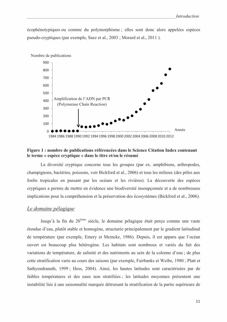
études (Fig. 1) ont mis en évidence une diversité cryptique c'est-à-dire que la diversité
génétique de nombreux organismes est bien supérieure à leur diversité morphologique. Ainsi,
les morpho-espèces correspondent à un regroupement de plusieurs espèces, identiques du
point de vue de la morphologie, appelées espèces cryptiques (Knowlton 1993 ; Norris, 2000 ;
Fenchel, 2005 ; Bickford et al., 2006). Ces espèces cryptiques peuvent toutefois présenter de
légères différences qui étaient jusqu’alors interprétées comme des variantes
_______________________________________________________________________Introduction
11
écophénotypiques ou comme du polymorphisme ; elles sont donc alors appelées espèces
pseudo-cryptiques (par exemple, Saez et al., 2003 ; Morard et al., 2011 ).
Figure 1 : nombre de publications référencées dans le Science Citation Index contenant
le terme « espèce cryptique » dans le titre et/ou le résumé
La diversité cryptique concerne tous les groupes (par ex. amphibiens, arthropodes,
champignons, bactéries, poissons, voir Bickford et al., 2006) et tous les milieux (des pôles aux
forêts tropicales en passant par les océans et les rivières). La découverte des espèces
cryptiques a permis de mettre en évidence une biodiversité insoupçonnée et a de nombreuses
implications pour la compréhension et la préservation des écosystèmes (Bickford et al., 2006).
Le domaine pélagique
Jusqu’à la fin du 20ième
siècle, le domaine pélagique était perçu comme une vaste
étendue d’eau, plutôt stable et homogène, structurée principalement par le gradient latitudinal
de température (par exemple, Emery et Meincke, 1986). Depuis, il est apparu que l’océan
ouvert est beaucoup plus hétérogène. Les habitats sont nombreux et variés du fait des
variations de température, de salinité et des nutriments au sein de la colonne d’eau ; de plus
cette stratification varie au cours des saisons (par exemple, Fairbanks et Weibe, 1980 ; Platt et
Sathyendranath, 1999 ; Hess, 2004). Ainsi, les hautes latitudes sont caractérisées par de
faibles températures et des eaux non stratifiées ; les latitudes moyennes présentent une
instabilité liée à une saisonnalité marquée détruisant la stratification de la partie supérieure de
0
100
200
300
400
500
600
700
800
900
1984 1986 1988 1990 1992 1994 1996 1998 2000 2002 2004 2006 2008 2010 2012
Amplification de l’ADN par PCR
(Polymerase Chain Reaction)
Année
Nombre de publications

_______________________________________________________________________Introduction
12
la colonne d’eau ; les régions équatoriales possèdent une stratification marquée, notamment
une thermocline nette et peu profonde (Rutherford et al., 1999). Le milieu pélagique reste
néanmoins un domaine vaste et il est difficile de distinguer des limites nettes entre ses
différentes parties. Certains auteurs ont proposé les fronts océaniques comme possibles
barrières, principalement pour le plancton (Rutherford et al., 1999 ; Boltovskoy et al., 2003),
mais ces fronts semblent loin d’être infranchissables comme le montre le maintien d’un flux
génique entre organismes planctoniques (foraminifères notamment) arctiques et antarctiques
(Norris et de Vargas, 2000).
Diversité cryptique en domaine pélagique
En 1994, Briggs estimait la diversité marine totale à 200 000 taxons (organismes
pluricellulaires), soit une diversité au moins 50 fois inférieure à celle du domaine terrestre qui
ne représente pourtant que 30% de la surface du globe. Cette faible diversité a été interprétée
comme résultant du fort potentiel de dispersion des organismes dans le milieu pélagique, ce
qui rend plus difficile la spéciation, en particulier si l’allopatrie en est la modalité principale
(Norris, 2000). Des études génétiques ont été réalisées sur des organismes pélagiques très
divers : bactéries (par ex. Moore et al., 1998), phytoplancton (par ex. Kooistra et al., 2008 ),
zooplancton (par ex. Laakmann et al., 2009 ; Bachy et al., 2013) ou ostéichtyens (par ex,
Miya et Nishida, 1997). Toutes montrent que la diversité cryptique est la règle chez les
organismes pélagiques. Cette découverte a bouleversé la perception du domaine pélagique en
montrant que la diversité des océans ouverts avait été largement sous-estimée. Pour expliquer
une telle diversité, il a fallu repenser les écosystèmes pélagiques comme un ensemble de
nombreuses niches écologiques abritant des espèces spécialisées (Laakmann et al., 2009 ;
Levine et HillRisLambers, 2009) ; les mécanismes de la spéciation sympatrique permettent
d’expliquer l’apparition d’espèces en l’absence de barrière physique et seraient donc
particulièrement à même de rendre compte de la spéciation en domaine pélagique (Norris,
2000; De Aguiar et al., 2009 ). La découverte de nombreuses espèces cryptiques a bien sûr eu
d’importantes répercussions : elle montre en particulier que l’inventaire de la biodiversité
marine est encore très incomplet et elle a des conséquences sur les mesures de conservation
des espèces et de leurs habitats, celles-ci étant plus spécialisées qu’initialement envisagé
(Bickford et al., 2006).

_______________________________________________________________________Introduction
13
2. Les foraminifères planctoniques
Les morpho-espèces de foraminifères planctoniques
Les foraminifères planctoniques sont des organismes unicellulaires du super-groupe
des Rhizaria (Adl et al., 2005). Omniprésents en milieu marin, ils occupent des niches
écologiques très diverses et font partie des proies du métazooplancton (Hemleben et al.,
1989). Ces « protozoaires » pélagiques sécrètent une coquille calcitique (aussi appelée test)
submillimétrique (<500 μm), faisant des foraminifères planctoniques un contributeur
important dans le cycle du carbone (Schiebel, 2002). Leur registre fossile s’étend du
Jurassique inférieur à l’Actuel (Hart et al., 2003). Les très vastes répartitions
biogéographiques des morpho-espèces de foraminifères planctoniques permettent des
corrélations biostratigraphiques à l’échelle mondiale et font donc des foraminifères
planctoniques d’excellents marqueurs pour reconstituer la chronologie des dépôts
sédimentaires pélagiques (Kenneth et Srinivasan, 1983). L’utilisation biostratigraphique des
foraminifères planctoniques, dès le XIXème siècle, explique que leur taxonomie repose
essentiellement sur la caractérisation de descripteurs morphologiques des tests (concept de
morpho-espèce) (Kennett et Srinivasan, 1983). Ce concept de morpho-espèce, hérité des
approches linnéennes et paléontologiques, prévaut toujours, à tel point que la majorité des
holotypes de taxons actuels sont des spécimens fossilisés (Bolli et Saunders, 1985). Cette
prééminence des caractères morphologiques dans la définition des espèces trouve aussi son
origine dans le fait que le critère d’interfécondité (concept d’espèce biologique) de ces
organismes n’a jamais pu être testé en laboratoire chez ces organismes difficiles à cultiver
(Hemleben et al., 1989). Néanmoins, dès le milieu du XXème siècle, la libération de
nombreuses cellules flagellées en fin de cycle a été observée chez des individus cultivés, ce
qui a conduit à supposer un cycle de vie sexué chez les foraminifères planctoniques
(Hemleben et al., 1989). Ce cycle de vie semble suivre une périodicité lunaire ou semi-lunaire
chez les espèces vivant en surface alors que les espèces plus profondes ont un cycle plus long,
pouvant atteindre une année (Schiebel et Hemleben, 2005).
_______________________________________________________________________Introduction
14
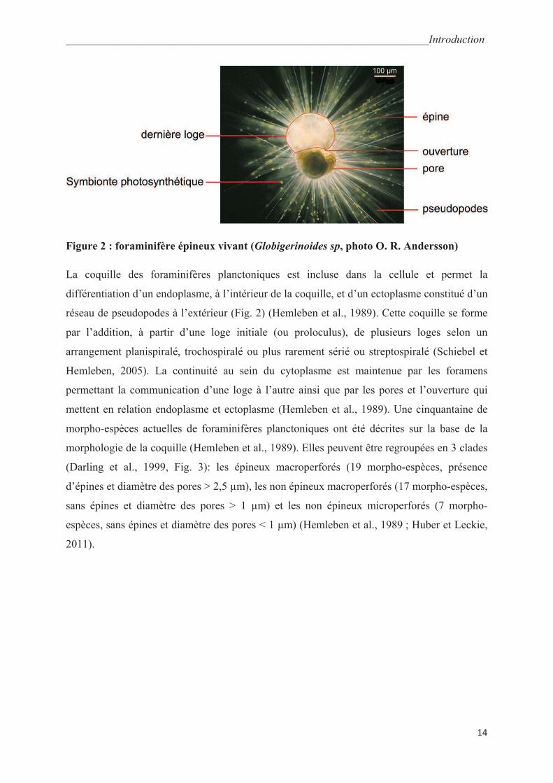
Figure 2 : foraminifère épineux vivant (Globigerinoides sp, photo O. R. Andersson)
La coquille des foraminifères planctoniques est incluse dans la cellule et permet la
différentiation d’un endoplasme, à l’intérieur de la coquille, et d’un ectoplasme constitué d’un
réseau de pseudopodes à l’extérieur (Fig. 2) (Hemleben et al., 1989). Cette coquille se forme
par l’addition, à partir d’une loge initiale (ou proloculus), de plusieurs loges selon un
arrangement planispiralé, trochospiralé ou plus rarement sérié ou streptospiralé (Schiebel et
Hemleben, 2005). La continuité au sein du cytoplasme est maintenue par les foramens
permettant la communication d’une loge à l’autre ainsi que par les pores et l’ouverture qui
mettent en relation endoplasme et ectoplasme (Hemleben et al., 1989). Une cinquantaine de
morpho-espèces actuelles de foraminifères planctoniques ont été décrites sur la base de la
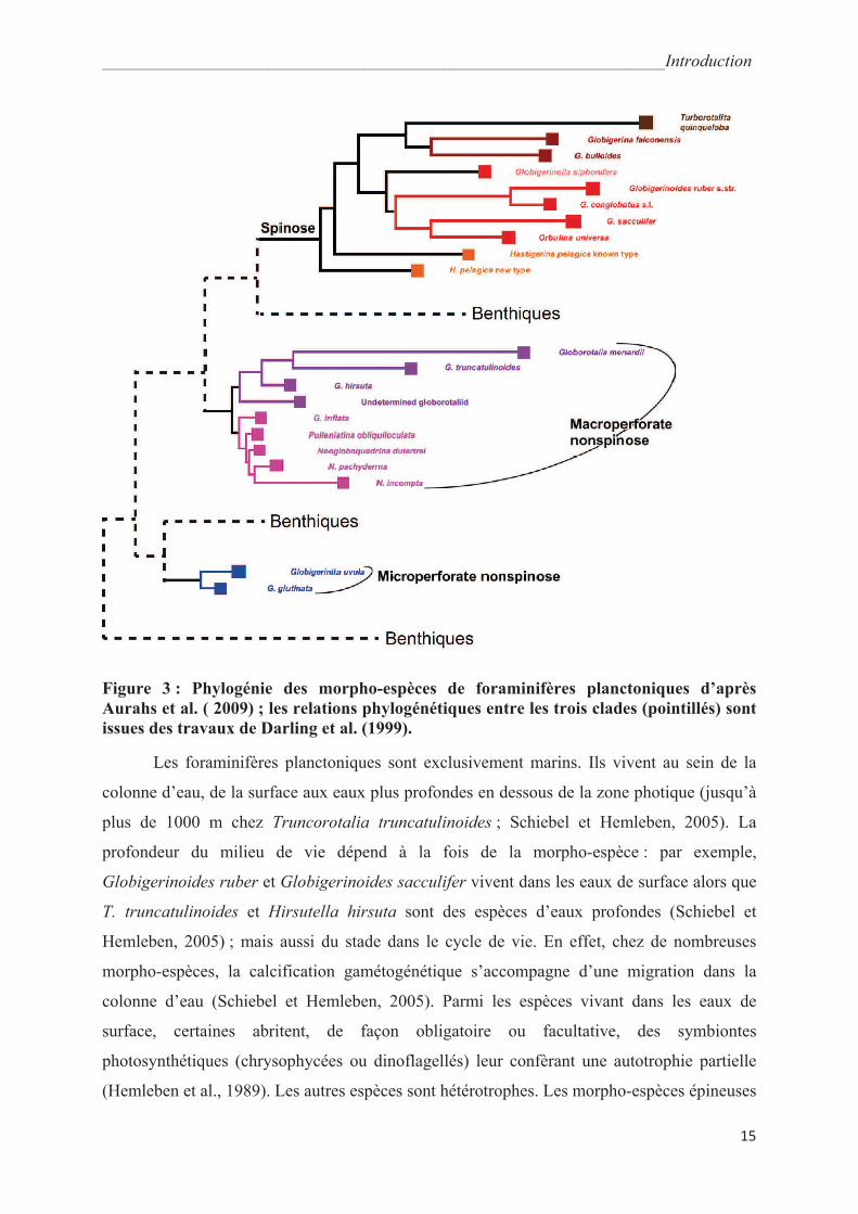
morphologie de la coquille (Hemleben et al., 1989). Elles peuvent être regroupées en 3 clades
(Darling et al., 1999, Fig. 3): les épineux macroperforés (19 morpho-espèces, présence
d’épines et diamètre des pores > 2,5 μm), les non épineux macroperforés (17 morpho-espèces,
sans épines et diamètre des pores > 1 μm) et les non épineux microperforés (7 morpho-
espèces, sans épines et diamètre des pores < 1 μm) (Hemleben et al., 1989 ; Huber et Leckie,
2011).
_______________________________________________________________________Introduction
15
Figure 3 : Phylogénie des morpho-espèces de foraminifères planctoniques d’après
Aurahs et al. ( 2009) ; les relations phylogénétiques entre les trois clades (pointillés) sont
issues des travaux de Darling et al. (1999).
Les foraminifères planctoniques sont exclusivement marins. Ils vivent au sein de la
colonne d’eau, de la surface aux eaux plus profondes en dessous de la zone photique (jusqu’à
plus de 1000 m chez Truncorotalia truncatulinoides ; Schiebel et Hemleben, 2005). La
profondeur du milieu de vie dépend à la fois de la morpho-espèce : par exemple,
Globigerinoides ruber et Globigerinoides sacculifer vivent dans les eaux de surface alors que
T. truncatulinoides et Hirsutella hirsuta sont des espèces d’eaux profondes (Schiebel et
Hemleben, 2005) ; mais aussi du stade dans le cycle de vie. En effet, chez de nombreuses
morpho-espèces, la calcification gamétogénétique s’accompagne d’une migration dans la
colonne d’eau (Schiebel et Hemleben, 2005). Parmi les espèces vivant dans les eaux de
surface, certaines abritent, de façon obligatoire ou facultative, des symbiontes
photosynthétiques (chrysophycées ou dinoflagellés) leur confèrant une autotrophie partielle
(Hemleben et al., 1989). Les autres espèces sont hétérotrophes. Les morpho-espèces épineuses
_______________________________________________________________________Introduction
16
hétérotrophes se nourrissent principalement de zooplancton (copépodes) (Caron et Bé, 1984)
alors que les morpho-espèces non épineuses privilégient le phytoplancton (Diatomées surtout)
(Spindler et al., 1984).
Taxonomie morphologique chez les foraminifères planctoniques
L’utilisation historique des foraminifères comme marqueurs stratigraphiques est à
l’origine de leur taxonomie basée sur la morphologie du test. L’aspect des coquilles,
extrêmement variable, peut être décrit principalement par la forme et agencement des loges, la
microstructure (épines, pustules, pores, carènes) et les caractéristiques de l’ouverture (Kennett
et Srinivasan, 1983). Néanmoins, la question du sens biologique et donc taxonomique de ces
caractères est cruciale (Parker, 1962). Par exemple, la dernière loge de forme allongée
(appelée « sac ») de Globigerinoides sacculifer a longtemps été utilisée comme principal
critère d’identification de cette morpho-espèce jusqu’à ce que des cultures (Bé, 1980 ; Bé et
al., 1983, Hemleben et al., 1987 ; Bijma et al., 1992) montrent que cette loge pourrait
correspondre à un stade ontogénétique facultatif, donc sans valeur taxonomique. La difficulté
d’observation de la microstructure des tests avant la généralisation des clichés MEB dans les
années 1970 (Hemleben et al., 1989) a entrainé de nombreux débats quant à la classification et
l’appartenance taxonomique des morpho-espèces. Ainsi, la morpho-espèce non épineuse
Neogloboquadrina pachyderma a longtemps été classée dans le genre épineux Globigerina
(par exemple, Banner et Blow, 1960). De même, certaines confusions entre stades juvéniles et
espèces n’ont pu être levées qu’à partir du développement des cultures et des études
ontogénétiques (par exemple, le cas de Globigerina bulloides var. borealis ; Bé, 1960).
Les classifications morphologiques actuelles (Kennett et Srinivasan, 1983, Hemleben
et al., 1989, Aze et al., 2011) recoupent largement les classifications phylogénétiques (Aurahs
et al., 2009). Elles délimitent les trois principaux clades de foraminifères planctoniques en se
basant sur la microstructure de la coquille : présence d’épines et aspect général de la porosité.
Au sein de ces clades, les morpho-espèces sont délimitées le plus souvent à l’aide de la forme
et de l’agencement des loges et des caractéristiques de l’ouverture. Néanmoins,
l’identification de la limite entre variations écophénotypiques au sein d’une espèce et
différences morphologiques entre espèces proches est un obstacle majeur pour ces taxonomies
basées uniquement sur la morphologie (Parker, 1962). Cette limite est d’autant plus difficile à
établir que l’on observe parfois des clines morphologiques (Hilbrecht, 1997). Ainsi, la
distinction entre Neogloboquadrina dutertrei, Neogloboquadrina incompta et N. pachyderma
_______________________________________________________________________Introduction
17
est restée longtemps problématique : certains, comme Cifelli (1961), les classaient comme des
espèces distinctes alors que d’autres, au contraire, les considéraient comme une seule espèce
présentant deux pôles morphologiques reliés par des « pachyderma-dutertrei intergrades »
(par exemple, Rohling et Gieskers, 1989 ; Parker et Berger, 1971). Finalement, les critères
morpho-anatomiques retenus semblent pertinents pour une classification à l’échelle des
morpho-espèces mais trouvent cependant leur limite chez les clades présentant d’importantes
variations intra-spécifiques.
Biogéographie des foraminifères planctoniques et applications
paléocéanographiques
Les foraminifères planctoniques occupent les eaux de l’océan mondial, de la banquise
antarctique (Neogloboquadrina pachyderma ; Dieckmann et al., 1991) aux eaux tropicales et
équatoriales (par exemple, Globigerinoides ruber ; Hemleben et al., 1989). Chaque morpho-
espèce présente des affinités environnementales qui lui sont propres et qui contrôlent donc sa
distribution biogéographique (Hilbrecht, 1996 ; Fig. 4). Ces affinités environnementales ont
été déduites de l’analyse des sédiments de surface (par exemple, Hilbrecht 1996), des récoltes,
parfois stratifiées, de foraminifères vivants grâce à des filets à plancton (par exemple, Bé,
1959) ainsi que d’expériences de culture en laboratoire (par exemple, Bé, 1980 ; Bijma et al.,
1992). Certaines morpho-espèces sont généralistes comme Globigerinita glutinata ou
Globigerina bulloides qui pourraient supporter des températures allant de presque 0°C à plus
de 30°C (Hilbrecht, 1996) alors que d’autres ont des affinités plus strictes comme G. ruber
pink qui est exclusivement tropicale (Hilbrecht, 1996). Dans le cas des espèces polaires à
tempérées on observe des distributions bipolaires (par exemple, N. pachyderma, Hemleben et
al., 1989).
_______________________________________________________________________Introduction
18
Figure 4 : affinités environnementales vis-à-vis de la température des principales
morpho-espèces de foraminifères planctoniques ; les épaisseurs du trait donnent les
abondances relatives (Darling et Wade, 2008, modifié de Bé et Tolderlund, 1971).
Les coquilles de foraminifères planctoniques représentent 30 à 80% du bilan carbonaté
profond ce qui explique leur registre fossile particulièrement complet et abondant (Schiebel et
Hemleben, 2005). Rutherford et al. (1999) ont montré que la répartition des assemblages de
morpho-espèces est corrélée aux conditions environnementales, et plus particulièrement à la
température et, dans une moindre mesure, à la productivité des eaux de surface. Les
foraminifères planctoniques sont donc à la fois abondants et sensibles aux changements
climatiques, ce qui en fait un groupe fondamental pour les reconstructions
paléocéanographiques. Les fonctions de transfert permettent de relier assemblages fossiles et
conditions paléoenvironnementales. Elles sont calibrées à partir des abondances relatives des
_______________________________________________________________________Introduction
19
tests des différentes morpho-espèces de foraminifères actuels recueillis dans les sédiments de
surface. Ces assemblages sont alors mis en relation avec la température mesurée à 10 m de
profondeur à la verticale des sédiments de surface (Kucera et al., 2005). D’après le principe
d’actualisme, ces fonctions de transfert restent valables tant que les morpho-espèces peuvent
être reconnues, en supposant que leurs caractéristiques éco-physiologiques et leurs
distributions géographiques sont restées stables au cours du temps. Elles permettent donc
l’estimation des paléotempératures océaniques, en particulier au cours du Quaternaire (Kucera
et al., 2005). Par ailleurs, les compositions isotopiques et élémentaires (18
O, 13
C, Mg/Ca,
Katz et al., 2010) des coquilles ont été empiriquement mises en relation avec les conditions
environnementales (le plus souvent, la température). Ces équations ont ensuite pu être
appliquées dans le registre fossile pour en déduire les caractéristiques des océans anciens
(pour une synthèse voir Katz et al., 2010).
Diversité cryptique chez les foraminifères planctoniques
La première séquence d’ADN de foraminifère planctonique a été obtenue par Merle et
al. (1994). Plus tard, Holzman et Pawlowski (1996) ont publié les premières méthodes
d’extraction et d’amplification par PCR spécifiquement adaptées aux foraminifères. Les
premières études génétiques ont eu pour objet principal la phylogénie des foraminifères
(benthiques et planctoniques) et la question de leur divergence possiblement très précoce aux
sein des eucaryotes (Pawlowski et al., 1996). Les premiers travaux portant sur la diversité
génétique au sein des morpho-espèces chez les foraminifères planctoniques datent de 1997
(de Vargas et al., 1997 ; Darling et al., 1997 ; Huber et al., 1997). A l’exception de quelques
rares séquences de régions codantes utilisées dans le cadre de phylogénies de foraminifères
(actine, Flakowski et al., 2005 ; ARN polymérase II, Longet et al., 2007), l’étude de la
diversité des foraminifères planctonique se base sur des séquences partielles de l’ADN
ribosomal 18S (SSU, petite sous-unité ribosomale) et des ITS (internal transcribed spacer)
(Fig. 5).

_______________________________________________________________________Introduction
20
Figure 5 : organisation de l’ADN ribosomal nucléaire et régions séquencées chez les
foraminifères planctoniques. Les rectangles correspondent aux régions transcrites
incorporées dans les ribosomes, les traits représentent les régions transcrites mais non
incorporées aux ribosomes. Les ordres de grandeur des tailles de la SSU et de l’ITS sont
donnés en paires de bases.
Darling et al. (1997) et de Vargas et al. (1997) ont montré que la SSU des
foraminifères est particulièrement longue et présente des boucles variables spécifiques à ce
groupe. De plus, cette région évolue de façon inhabituellement rapide (30 à 50 fois plus vite
que chez les métazoaires ; de Vargas et al., 1997) ce qui en fait un bon marqueur pour étudier
la diversité génétique au sein des morpho-espèces. L’ITS est une région transcrite non
incorporée aux ribosomes et qui évolue donc à un rythme encore plus rapide que la SSU.
Cette région n’a été jusqu’à présent étudiée que chez deux morpho-espèces, T.
truncatulinoides et Globoconella inflata (de Vargas et al., 2001 ; Morard et al., 2011).
Les séquences de la fin de la SSU ont permis de proposer une phylogénie des morpho-
espèces de foraminifères planctoniques (Aurahs et al., 2009). Ces derniers forment un groupe
polyphylétique au sein des foraminifères benthiques (Fig. 3) ; les trois groupes (macroperforés
épineux, macroperforés non épineux et microperforés) correspondent chacun à un clade
différent (Darling et al., 1999 ; Aurahs et al., 2009).
Les études se focalisant sur la diversité génétique au sein des morpho-espèces (tableau
1) ont montré que la diversité génétique des foraminifères planctoniques ne fait pas exception
à la règle dans le domaine pélagique. Parmi la cinquantaine de morpho-espèces décrites
(Hemleben et al., 1989), 11 ont été étudiées avec obtention de nombreuses séquences
d’individus provenant d’environnements contrastés et géographiquement éloignés. Ces 11
morpho-espèces sont en réalité constituées d’un ensemble de 2 à 7 types génétiques pouvant
correspondre à des espèces cryptiques (Tableau 1).
_______________________________________________________________________Introduction
21
morphoespèce nombre de génotypes marqueur génétique utilisé références
Neogloboquadrina pachyderma 7 SSUrDNA 4,6,8
Turborotalia quinqueloba 6 SSUrDNA 4,5,9
Neogloboquadrina incompta 2 SSUrDNA 4,6,7
Globigerina bulloides 7 SSUrDNA 3,4,5,8
Truncorotalia truncatulinoides 5 SSUrDNA et ITSrDNA 10,12,14
Orbulina universa 3 SSUrDNA 1,2,10,11
Globigerinella siphonifera 7 SSUrDNA 1,2,3
Globigerinoides ruber 5 SSUrDNA 1,2,3,10
Globoconella inflata 2 ITSrDNA 13
Hastigerina pelagica 3 SSUrDNA 15
Pulleniatina obliquiloculata 3 SSUrDNA 16
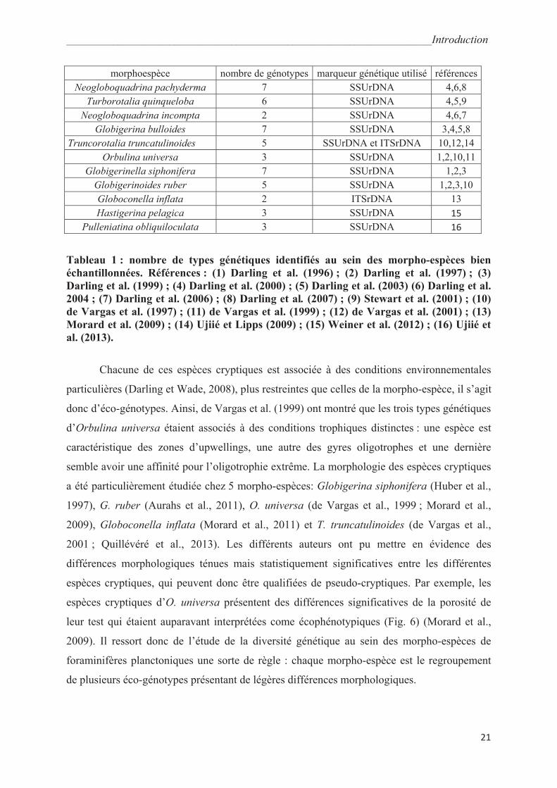
Tableau 1 : nombre de types génétiques identifiés au sein des morpho-espèces bien
échantillonnées. Références : (1) Darling et al. (1996) ; (2) Darling et al. (1997) ; (3)
Darling et al. (1999) ; (4) Darling et al. (2000) ; (5) Darling et al. (2003) (6) Darling et al.
2004 ; (7) Darling et al. (2006) ; (8) Darling et al. (2007) ; (9) Stewart et al. (2001) ; (10)
de Vargas et al. (1997) ; (11) de Vargas et al. (1999) ; (12) de Vargas et al. (2001) ; (13)
Morard et al. (2009) ; (14) Ujiié et Lipps (2009) ; (15) Weiner et al. (2012) ; (16) Ujiié et
al. (2013).
Chacune de ces espèces cryptiques est associée à des conditions environnementales
particulières (Darling et Wade, 2008), plus restreintes que celles de la morpho-espèce, il s’agit
donc d’éco-génotypes. Ainsi, de Vargas et al. (1999) ont montré que les trois types génétiques
d’Orbulina universa étaient associés à des conditions trophiques distinctes : une espèce est
caractéristique des zones d’upwellings, une autre des gyres oligotrophes et une dernière
semble avoir une affinité pour l’oligotrophie extrême. La morphologie des espèces cryptiques
a été particulièrement étudiée chez 5 morpho-espèces: Globigerina siphonifera (Huber et al.,
1997), G. ruber (Aurahs et al., 2011), O. universa (de Vargas et al., 1999 ; Morard et al.,
2009), Globoconella inflata (Morard et al., 2011) et T. truncatulinoides (de Vargas et al.,
2001 ; Quillévéré et al., 2013). Les différents auteurs ont pu mettre en évidence des
différences morphologiques ténues mais statistiquement significatives entre les différentes
espèces cryptiques, qui peuvent donc être qualifiées de pseudo-cryptiques. Par exemple, les
espèces cryptiques d’O. universa présentent des différences significatives de la porosité de
leur test qui étaient auparavant interprétées come écophénotypiques (Fig. 6) (Morard et al.,
2009). Il ressort donc de l’étude de la diversité génétique au sein des morpho-espèces de
foraminifères planctoniques une sorte de règle : chaque morpho-espèce est le regroupement
de plusieurs éco-génotypes présentant de légères différences morphologiques.

_______________________________________________________________________Introduction
22
Figure 6 : Vues de détail au microscope électronique à balayage de la face interne des
tests des trois espèces cryptiques d’Orbulina universa (Morard et al., 2009)
Implications paleocéanographiques de la mise en évidence d’une diversité
cryptique chez les foraminifères planctoniques
La présence d’espèces pseudo-cryptiques a des conséquences sur les reconstitutions
paléoenvironnementales basées sur les foraminifères planctoniques. Les méthodes employées,
fonctions de transfert ou équations de paléotempérature font implicitement l’hypothèse que
les morpho-espèces ont chacune des affinités écologiques homogènes. Or, ces fonctions de
transfert utilisent en fait des morpho-espèces qui sont constituées de plusieurs types
génétiques ayant chacun des exigences écologiques qui leur sont propres. Ceci entraine une
augmentation de la variance thermique et donc un accroissement des marges d’erreur et
même, une sur- ou sous-estimation des paléotempératures si une ou plusieurs espèces
cryptiques sont absentes de la base de données utilisée pour la calibration des fonctions de
transfert. Les reconstitutions paléocéanographiques du Quaternaire, largement basées sur les
fonctions de transfert perdent alors en précision (Kucera et Darling, 2002 ; Kucera et al.,
2005). Les équations de calibration en géochimie, pour le 18
O, le 13
C et le rapport Mg/Ca,
sont réalisées à partir d’individus appartenant à la même morpho-espèce, mais les différentes
espèces cryptiques la constituant ne sont pas prises en compte (Erez et Luz, 1983 ; Anand et
Elderfield, 2003). Or, des individus provenant d’espèces cryptiques différentes pourraient
avoir des fractionnements isotopiques ou élémentaires différents (Darling et Wade, 2008), ce
qui augmenterait la marge d’erreur des équations et donc des reconstructions, voire biaiserait
systématiquement les estimations de paléotempératures si ces équations sont appliquées à des
espèces cryptiques n’ayant pas été prises en compte dans les calibrations.
.
_______________________________________________________________________Introduction
23
Cependant, comme il semble que les espèces cryptiques de foraminifères
planctoniques correspondent généralement à des éco-génotypes et des espèces pseudo-
cryptiques, il est possible de transformer cet obstacle de la diversité cryptique en une
opportunité d’améliorer les reconstructions paléoclimatiques. Connaissant les affinités
environnementales actuelles des espèces cryptiques, il devient possible d’intégrer les
préférences environnementales propres aux génotypes dans la calibration des fonctions de
transfert. Les affinités thermiques correspondant aux espèces sont alors plus réduites, ce qui
permet de reconstituer de façon plus précise la température des eaux de surface anciennes.
Kucera et Darling (2002) ont ainsi estimé que pour les meilleures reconstitutions, la marge
d’erreur pourrait passer en dessous d’1°C, précision maximale des fonctions de transfert
basées sur les morpho-espèces (Malmgren et al., 2001). Depuis, Morard et al. (2013) ont
montré que l’intégration de la diversité cryptique de seulement 4 morpho-espèces
(Globigerina bulloides, Orbulina universa, Truncorotalia truncatulinoides et Globoconella
inflata) suffisait à réduire la marge à moins de 1°C dans l’application de fonctions de transfert
dans l’hémisphère sud. De même, calibrer les équations de paléo-températures basées sur les
compostions isotopiques et élémentaires à partir des espèces cryptiques permettra de réduire
le bruit du aux différences d'affinité écologiques entre espèces. Comme d’après les horloges
moléculaires certaines spéciations cryptiques ont eu lieu il y a plusieurs millions d’années (6 à
12 Ma pour O. universa ; de Vargas et al., 1999 ), l’amélioration des reconstitutions
paléoclimatiques basées sur les foraminifères planctoniques est donc possible pour les
derniers millions d’années et plus particulièrement pour le Pléistocène-Holocène dont le
spectre de morpho-espèces est sensiblement identique à celui de l’Actuel.

_______________________________________________________________________Introduction
24
3. Objectifs
L’objectif de cette thèse est de poursuivre l’investigation de la diversité pseudo-
cryptique chez les foraminifères planctoniques. Cette investigation implique la mise en
relation de la taxonomie moléculaire, c’est-à-dire les différents types génétiques décrits à
partir d’individus actuels, avec la morpho-taxonomie qui est la seule utilisable dans le registre
fossile.
Délimitation des espèces chez les foraminifères planctoniques
La première partie de mon travail a pour but : (1) de proposer et de comparer des
méthodes quantitatives de délimitation des espèces à partir des séquences d’ADN ; (2) de
faire une mise au point taxonomique des espèces cryptiques chez les foraminifères
planctoniques à partir des séquences déposées sur NCBI augmentées de nouvelles données et
(3) de réaliser une synthèse des données biogéographiques associées à cette nouvelle
taxonomie. Le découpage des morpho-espèces en espèces cryptiques a été jusqu’à présent
défini de façon qualitative à partir des groupements de séquences observés sur les arbres
phylogénétiques. Ces définitions sont donc subjectives et de nombreux auteurs ont décrit des
« génotypes », « types » et « sous-types » dont le rang taxonomique (c’est-à-dire, espèce,
sous-espèce ou population) n’est pas clairement établi (Kucera et Darling, 2002). Or,
l’utilisation des espèces cryptiques en paléocéanographie requiert une grande cohérence
taxonomique. De plus, la mise au point d’un cadre de référence permettant la définition des
espèces cryptiques à partir des séquences ADN ouvre la voie à l’interprétation des jeux de
données issus du séquençage environnemental, qui est une fabuleuse opportunité de dévoiler
la biogéographie des espèces cryptiques.
Phylogénies basées sur des séquences complètes de la SSU
Les relations phylogénétiques entre les types génétiques de quelques morpho-espèces
et/ou le statut taxonomique de leurs différents types génétiques restent encore mal résolus.
Dans ces cas particuliers, les séquences partielles de la SSU semblent donc insuffisamment
informatives. Pourtant, les séquences complètes de la SSU restent très rares chez les
foraminifères planctoniques (Schweizer et al., 2008 ; Seears, 2011). De plus, ces séquences,
utilisées uniquement dans le cadre de phylogénies à l’échelle des principaux clades, ne
permettent pas l’étude de la diversité cryptique au sein des morpho-espèces. En réalisant, pour
la première fois, le séquençage de la SSU complète des Types II, III et IV de
_______________________________________________________________________Introduction
25
Neogloboquadrina pachyderma, nous allons mettre en évidence l’intérêt des séquences
complètes de la SSU pour des phylogénies à l’échelle de la morpho-espèce.
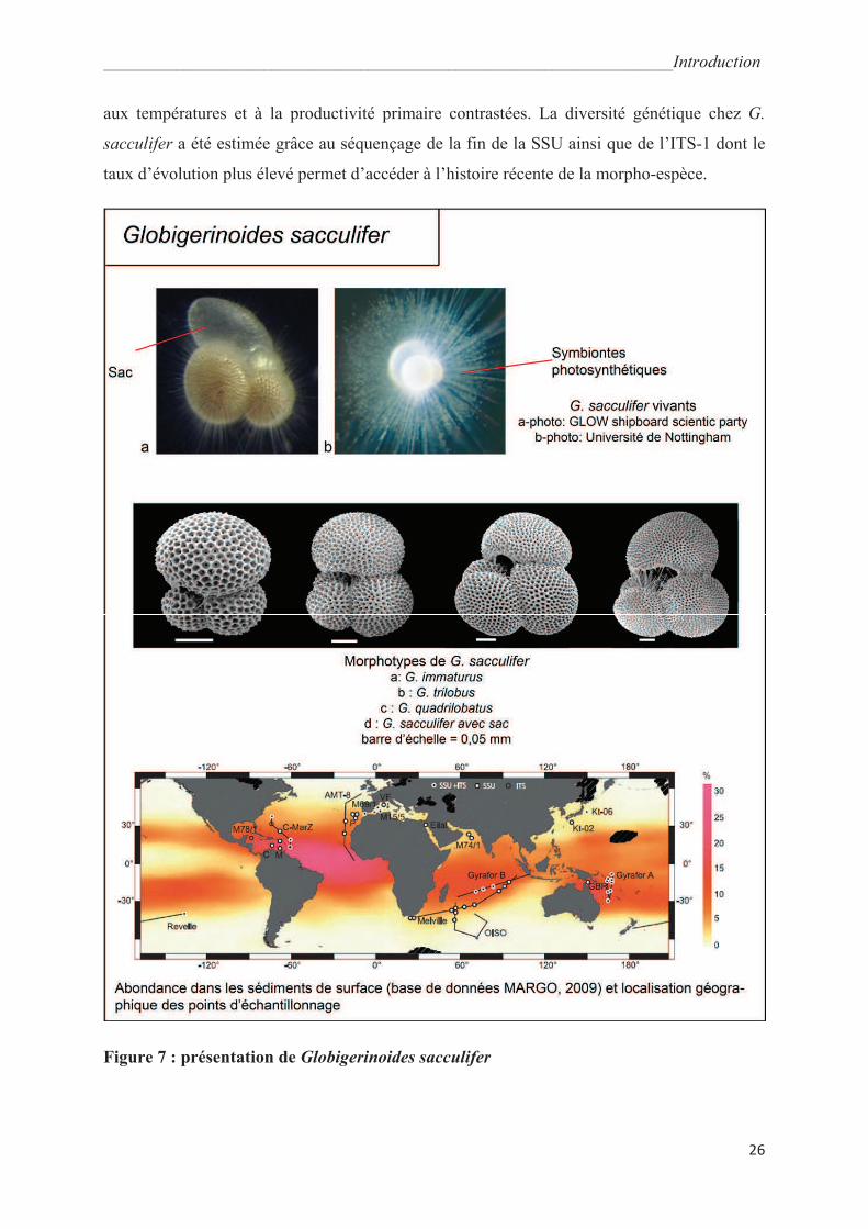
Diversité cryptique au sein de la morpho-espèce Globigerinoides sacculifer
Ce troisième chapitre s’intéresse à la morpho-espèce Globigerinoides sacculifer dont
la diversité génétique est encore sous-échantillonnée. Globigerinoides sacculifer est un
foraminifère planctonique épineux de la super-famille des Globigerinoidea (groupe des
foraminifères macroperforés épineux : Schiebel et Hemleben, 2005). Il est apparu au Miocène
inférieur il y a 19,3 à 18,7 Ma (Kennett et Srinivasan, 1983 ; Berggren et al., 1995) ce qui en
fait une des plus anciennes morpho-espèces encore présentes actuellement. Le test de G.
sacculifer est trochospiralé avec des loges sphériques sauf la dernière, appelée le « sac » qui
peut présenter une élongation distale très typique (Fig. 7). Il possède en outre une
microstructure en nid d’abeille caractéristique. Ce foraminifère est très abondant (base de
données du Projet Margo, 2009, Fig. 7) dans les eaux tropicales et sub-tropicales et supporte
d’assez larges gammes de température et de salinité : de 14°C à 31°C et de 24‰ à 47‰ avec
une température optimale de croissance de 28°C (Hemleben et al., 1989 ; Bijma et al., 1990).
Globigerinoides sacculifer vit dans la partie supérieure de la zone photique (20-30m) durant
la majeure partie de son développement où il profite d’une autotrophie partielle grâce à
l’activité photosynthétique de ses symbiontes (le dinoflagellé Gymnodinium bei ; Gast et
Caron, 1996). Bé et Hemleben (1970) interprètent la calcification gamétogénétique et la perte
des épines qui lui est associée comme un alourdissement du test permettant au foraminifère de
couler et donc de se reproduire plus en profondeur dans la colonne d’eau.
Du fait de sa grande abondance, G. sacculifer est une espèce-clef pour les
reconstructions paléocéanographiques des régions de basse latitude. Cette espèce a aussi été
utilisée pour calibrer des équations de paléotempérature basées sur le 18
O (Erez et Luz, 1983)
et le rapport Mg/Ca (Nurnberg et al., 1996). De plus, la diversité morphologique est
particulièrement importante chez cette morpho-espèce, ce qui a conduit à la prolifération des
termes taxonomiques : G. sacculifer avec sac ; G. sacculifer sans sac, G. trilobus, G. trilobus
immaturus, G. quadrilobatus (Hemleben et al., 1987). De par ses larges affinités écologiques
et sa grande diversité morphologique, il semble a priori très probable que G. sacculifer soit un
regroupement de morphotypes correspondant à différents éco-génotypes. Cette étude se
propose de tester cette hypothèse en se basant sur un large panel d’échantillons, incluant les
différents morphotypes connus, en provenance des différents bassins océaniques et de régions
_______________________________________________________________________Introduction
26
aux températures et à la productivité primaire contrastées. La diversité génétique chez G.
sacculifer a été estimée grâce au séquençage de la fin de la SSU ainsi que de l’ITS-1 dont le
taux d’évolution plus élevé permet d’accéder à l’histoire récente de la morpho-espèce.
Figure 7 : présentation de Globigerinoides sacculifer

_______________________________________________________________________Introduction
27
Biogéographie et caractérisation morphologique des génotypes de
Neogloboquadrina pachyderma
La difficile observation de la microstructure des foraminifères planctoniques avant la
généralisation des clichés MEB, dans les années 1970, a généré beaucoup de confusions quant
à l’identité taxonomique de Neogloboquadrina pachyderma. Cette morpho-espèce a été
initialement intégrée au genre épineux Globigerina (d’Orbigny, 1846), et ce n’est qu’avec les
premiers clichés précis de la surface du test que l’appartenance de ce foraminifère au groupe
des macroperforés a été démontrée (Collen et Vella, 1973). Les références à « Globigerina »,
« Globoquadrina » ou « Globorotalia » pachyderma ne sont tombées en désuétude qu’au
début des années 1980 (Kennett et Srinivasan, 1983), au profit de Neogloboquadrina
pachyderma. En disséquant des N. pachyderma matures, Bé (1960) a montré que les individus
traditionnellement diagnostiqués comme des Globigerina bulloides atypiques correspondaient
en fait aux juvéniles de N. pachyderma.
Par ailleurs, la distinction entre N. pachyderma et ses proches parents
Neogloboquadrina incompta (= N. pachyderma dextre) et N. dutertrei est restée longtemps
problématique. Certains auteurs comme Ciffeli (1961) considéraient ces morpho-espèces
comme suffisamment différentes morphologiquement pour être considérées comme des
espèces distinctes alors que la plupart les considéraient comme une seule espèce avec deux
pôles morphologiques reliés par des formes intermédiaires (par exemple, Parker et Berger,
1971). Cette question n’a été définitivement tranchée que grâce aux analyses génétiques de
Darling et al. (2003) : N. pachyderma dextre que l’on trouve dans les eaux tempérées, et N.
pachyderma sénestre d’affinités sub-polaires à polaires (Hemleben et al., 1989) correspondent
à deux espèces clairement distinctes. Le morphotype dextre doit donc être nommé
Neogloboquadrina incompta (Darling et al., 2006). Dans mon travail, le nom N. pachyderma
ne s’applique donc qu’au morphotype à enroulement sénestre.
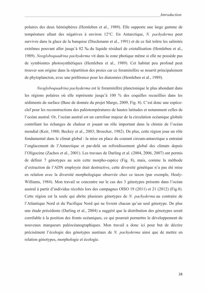
Neogloboquadrina pachyderma (Fig. 8) est un foraminifère planctonique du groupe
des macroperforés sans épines. Ses loges sont globuleuses et présentent un enroulement
sénestre suivant une trochospire comprimée. Le test de la forme mature possède 4 à 5 loges
sur le dernier tour et est épais avec des pores réduits suite à un encroutement de calcite qui lui
donne une silhouette sub-quadrangulaire caractéristique (Kennett et Srinivasan, 1983). Le
clade formé par N. pachyderma et N. incompta a divergé au Miocène supérieur, il y a 11,2
Ma (Aze et al., 2011). Neogloboquadrina pachyderma vit dans les eaux sub-polaires à
_______________________________________________________________________Introduction
28
polaires des deux hémisphères (Hemleben et al., 1989). Elle supporte une large gamme de
température allant des négatives à environ 12°C. En Antarctique, N. pachyderma peut
survivre dans la glace de la banquise (Dieckmann et al., 1991) et de ce fait tolère les salinités
extrêmes pouvant aller jusqu’à 82 ‰ du liquide résiduel de cristallisation (Hemleben et al.,
1989). Neogloboquadrina pachyderma vit dans la zone photique même si elle ne possède pas
de symbiontes photosynthétiques (Hemleben et al., 1989). Cet habitat peu profond peut
trouver son origine dans la répartition des proies car ce foraminifère se nourrit principalement
de phytoplancton, avec une préférence pour les diatomées (Hemleben et al., 1989).
Neogloboquadrina pachyderma est le foraminifère planctonique le plus abondant dans
les régions polaires où elle représente jusqu’à 100 % des coquilles recueillies dans les
sédiments de surface (Base de donnée du projet Margo, 2009, Fig. 8). C’est donc une espèce-
clef pour les reconstructions des paléotempératures de hautes latitudes et notamment celles de
l’océan austral. Or, l’océan austral est un carrefour majeur de la circulation océanique globale
contrôlant les échanges de chaleur et jouant un rôle important dans la chimie de l’océan
mondial (Keir, 1988; Beckey et al., 2003; Broecker, 1982). De plus, cette région joue un rôle
fondamental dans le climat global : la mise en place du courant circum-antarctique a entrainé
l’englacement de l’Antarctique et par-delà un refroidissement global des climats depuis
l’Oligocène (Zachos et al., 2001). Les travaux de Darling et al. (2004, 2006, 2007) ont permis
de définir 7 génotypes au sein cette morpho-espèce (Fig. 8), mais, comme la méthode
d’extraction de l’ADN employée était destructive, cette diversité génétique n’a pas été mise
en relation avec la diversité morphologique observée chez ce taxon (par exemple, Healy-
Williams, 1984). Mon travail se concentre sur le cas des 3 génotypes présents dans l’océan
austral à partir d’individus récoltés lors des campagnes OISO 19 (2011) et 21 (2012) (Fig.8).
Cette région est la seule qui abrite plusieurs génotypes de N. pachyderma au contraire de
l’Atlantique Nord et du Pacifique Nord qui ne livrent chacun qu’un seul génotype. De plus
une étude précédente (Darling et al., 2004) a suggéré que la distribution des génotypes serait
corrélable à la position des fronts océaniques, ce qui pourrait permettre le développement de
nouveaux marqueurs paléocéanographiques. Mon travail a donc ici pour but de décrire
précisément l’écologie des génotypes austraux de N. pachyderma ainsi que de mettre en
relation génotypes, morphologie et écologie.

_________________________________________________________________Introduction
29
Figure 8 : présentation de Neogloboquadrina pachyderma
30
PARTIE I
TAXONOMIE MOLECULAIRE CHEZ LES
FORAMINIFERES PLANCTONIQUES

________________________________________________________________________Partie I Chapitre 1
31
Chapitre 1 : taxonomie moléculaire chez les
foraminifères planctoniques, élaboration d’un
référentiel
Ce premier chapitre a pour objectif de discuter du rang taxonomique des
« génotypes », « types », « types génétiques » ou « espèces cryptiques » de foraminifères
planctoniques définis par la littérature et dont des séquences, correspondant à la fin de la SSU
(petite sous-unité ribosomique), sont disponibles à partir de la base de données NCBI. La
définition des unités taxonomiques chez les foraminifères planctoniques souffre en effet d’un
manque de critères objectifs. Ceci a entrainé une hétérogénéité des rangs taxonomiques entre
les différents types génétiques décrits par la littérature comme le montre l’analyse des
distances patristiques au sein des différentes morpho-espèces. Ce chapitre teste deux
méthodes quantitatives complémentaires et indépendantes, ABGD (Automatic Barcode Gap
Detection, Puillandre et al., 2012) et GMYC (Generalized Mixed Yule Coalescent, Pons et al.,
2006) permettant la définition objective d’unités taxonomiques. Ces méthodes permettent
l’élaboration d’une taxonomie de référence qui est confrontée aux données biogéographiques
et morphologiques disponibles. Néanmoins une utilisation généralisée et optimale de ces
méthodes quantitatives nécessite une standardisation des méthodes d’obtention des séquences.
Ces séquences doivent être suffisamment longues, homologues et nombreuses ; le séquençage
de plusieurs clones issus du même individu permet de détecter les cas de sur-découpage des
morpho-espèces.
Mots-clefs : espèces, unités taxonomiques, foraminifères planctoniques, distances
patristiques, ABGD, GMYC, biogéographie
Fiches-méthodes : VIII
Ce manuscrit va être soumis prochainement à PLoS One
Ont participé à ce manuscrit : Aurore ANDRE (analyses, interprétation, rédaction,
illustration), Raphael MORARD (récolte des données, illustration), Frédéric QUILLEVERE
(interprétation, rédaction), Christophe DOUADY (interprétation, rédaction), Yurika UJIIE
(acquisition de séquences).
________________________________________________________________________Partie I Chapitre 1
32
SSU rDNA divergence in planktonic foraminifera: molecular
taxonomy and biogeographic implications
Abstract
Ribosomal small subunit (SSU) DNA analyses have revealed that most of the modern
morpho-species of planktonic foraminifera are composed of a complex of several distinct
genetic types that may correspond to cryptic species. These genetic types are usually
delimitated using partial sequences located at the 3’end of the SSU, but these delimitations are
empirical and inherently subjective. Here, on the basis of patristic distances values calculated
within and among genetic types of 24 morpho-species of planktonic foraminifera, we show
that the taxonomic level of these genetic types is not homogenous and has been even
sometimes inconsistently defined. In order to further evaluate the species status of these
genetic types, we apply two quantitative and independent methods, ABGD (Automatic
Barcode Gap Detection) and GMYC (General Mixed Yule Coalescent), to a dataset of
published and newly obtained sequences located at the 3’ end of the SSU. Results of these
complementary approaches are highly congruent and lead to a molecular taxonomy that
qualify 49 genetic types of planktonic foraminifera as genuine (pseudo)cryptic species.
Our results advocate for a standardized sequencing procedure allowing objective and
homogenous delimitations of the (pseudo)cryptic species of planktonic foraminifera. Since
our data have also significant repercussions for our knowledge of planktonic foraminiferal
biogeography, we finally provide an updated integrative taxonomy in which we synthesize
geographic, ecological and morphological differentiations that can occur among the genuine
(pseudo)cryptic species. Due to molecular, environmental or morphological data scarcities,
many aspects of our proposed integrative taxonomy remain unclear. On the other hand, our
study opens up the challenging potential for a correct interpretation of environmental datasets
that may overcome open-ocean sampling insufficiency.
Key-words: cryptic species, taxonomic units, planktonic foraminifera, patristic distances,
ABGD, GMYC, biogeography
________________________________________________________________________Partie I Chapitre 1
33
1. Introduction
Fossil shells of planktonic foraminifera constitute one of the most informative archive
of changes in biodiversity that are used as a proxy to reconstruct past ocean conditions (e.g.,
Kucera, 2007). Since these reconstructions are empirically derived from species-specific
calibrations between extant environmental parameters and the abundance or chemical
composition of shells of modern individual species, they require an accurate taxonomic
consistency and a precise assessment of the biogeography and ecology of species (Kucera et
al., 2005; Katz et al., 2010; Morard et al., 2013). Yet, very little is known about the biology of
planktonic foraminifera (Lee and Andersson, 1991; Hemleben et al., 1989). Consequently,
following the paleontological use, the taxonomy of living species has been solely defined
based on diagnostic characters of their shells (morpho-species concept), occasionally
described from fossil type specimens extracted from sediments (Kennett and Srinivasan,
1983; Bolli and Saunders, 1985).
Molecular analyses revealed that the morphological taxonomy in planktonic
foraminifera led to underestimating biodiversity (for a review, see Darling and Wade, 2008).
Ribosomal SSU (Small Sub-Unit) sequences are usually used for phylogeny involving high
taxonomic ranks (e.g., Pace et al., 1986; Cavalier-Smith and Chao, 2003), but extensive
sequencing in planktonic foraminifera revealed an unexpected high rate of substitution within
these organisms, making this region of rDNA a suitable marker for studying genetic diversity
within and among closely related species (Darling et al., 1996; de Vargas et al., 1997;
Pawlowski et al., 1997; Pawlowski, 2000). Sequences of the even faster evolving region of
the ITS were also obtained for three morpho-species: Truncorotalia truncatulinoides (de
Vargas et al., 2001), Globoconella inflata (Morard et al., 2011) and Globigerinoides
sacculifer (André et al., 2013). Despite numerous attempts, mitochondrial genes such as COI,
which are often regarded as most convenient molecular targets for putative species
delimitation, are still unknown for those taxa. As a consequence, the SSU rDNA is for the
time being the most widely used marker for putative species delimitation in planktonic
foraminifera. Among the 24 morpho-species for which rDNA sequences are available, 49
genetic types, variously labeled “genotypes”, “types”, “subtypes” or “cryptic species” have
been published so far (NCBI database, January 17th
2013). Apart from one exception (André
et al., 2013), the studied morpho-species comprise more than one and up to seven distinct
genetic types (Darling and Wade, 2008; Aurahs et al., 2009a; 2011; Morard et al., 2011),
________________________________________________________________________Partie I Chapitre 1
34
several of which exhibiting a distinct biogeography and/or ecology (de Vargas et al., 1999;
2001; 2002; Darling et al., 1999; 2003; 2004; 2007; Weiner et al., 2012). Most of these
genetic types have been further suggested to be reproductively isolated and have thus been
considered as cryptic or rather pseudo-cryptic species when subtle differences in shell
morphology were detected (Huber et al., 1997; Morard et al., 2009; 2011; Aurahs et al.,
2011).
Nevertheless, a number of genetic types within a morpho-species, or a number of
“subtypes” within a genetic type, exhibit at least partially or even totally sympatric
distributions and/or similar shell morphologies (Darling and Wade., 2008; Kuroyanagi et al.,
2008; Aurahs et al., 2011; Weiner et al., 2012; Quillévéré et al., 2013). Many genetic types
have been solely defined on the basis of genetic differences without any additional DNA-
independent investigation that may help validating their species status. Such difficulties,
associated with the ongoing exponential increase of SSU rDNA sequences available, calls for
the development of a standardized protocol to help species delimitation using DNA
sequences. Definitions of the published genetic types through the last 15 years are the result
of subjective delimitations of sequences clusters, making their direct comparison rather
speculative. Most of these delimitations are based on studies at the morpho-species level
mainly because of the high and variable SSU rDNA substitution rates among planktonic
foraminifera, which induced highly ambiguous sequence alignments when datasets include
loosely related species (Aurahs et al., 2009b). Furthermore and because no common primers
have been found, sequences available are heterogeneous in length and cover different parts of
the 3’ end of the SSU region. Assessed altogether, this explains why no molecular threshold
has ever been discussed in the case of planktonic foraminifera.
A first empirical, quantitative approach of species delimitation using a clustering
method has been attempted by Görker et al. (2010). Although the resulting optimized
taxonomic units were mostly in agreement with those determined based on a morphological
taxonomy, this attempt failed to separate several morphologically highly divergent morpho-
species (e.g., Neogloboquadrina dutertrei and Pulleniatina obliquiloculata) and some well-
supported genetic types now recognized as pseudo-cryptic species (e.g., those of Orbulina
universa; de Vargas et al., 1999; Morard et al., 2009). Furthermore, such clustering-based
solution is not actually appropriate for molecular threshold definition and genetic type
delimitation, as the taxonomic level of the resulting classification directly relies on the design
of the reference dataset.
________________________________________________________________________Partie I Chapitre 1
35
In this paper, using patristic distances calculations among genetic types, we first
evaluate the consistency of empirical genetic type definitions. Such an evaluation is based on
the assumption that within a given morpho-species, the genetic types validate a species status
as soon as distances values are smaller within than among genetic types (Lefébure et al.,
2006; Puillandre et al., 2012a). This approach has limitations because 16 of the previously
defined genetic types are known from only one rDNA sequence, preventing any calculation of
distances within genetic types. Furthermore, sequences that lack genetic type assignation in
sequence databases such as GenBank, or for which a genetic type could not be inferred from
original publication, could not be considered for patristic distance calculations. Consequently,
we secondly test two independent and complementary automatic methods for molecular
operational taxonomic unit (MOTU) delimitations: the Automatic Barcode Gap Delimitation
(ABGD; Puillandre et al., 2012a), which allows calculation of genetic distances within and
among genetic types, and the General Mixed Yule Coalescent (GMYC; Pons et al., 2006),
which uses phylogenetic trees to determine the transition signal from coalescent to speciation
branching patterns. These methods provide alternative delimitations and offer the opportunity
to analyze sequences that lack former assignation in their genetic type. Finally, we confront
the results of the different methods in order to establish which of the previously and newly
defined genetic types may correspond to genuine species. This molecular taxonomy has
significant implications for our knowledge of planktonic foraminiferal species biogeography.
We consequently propose an updated integrative taxonomy (Dayrat, 2005; de Quieroz, 2007;
Puillandre et al., 2012b) of modern planktonic foraminifera, in which biogeographical,
ecological and/or morphological differentiations that can occur among species validated as
genuine are synthetized.
________________________________________________________________________Partie I Chapitre 1
36
2. Material
Putative species delimitations relying implicitly or explicitly on genetic distances
should be based on the same genetic marker to insure that they correspond to the same
taxonomic level (e.g., Coleman, 2003; Logares et al., 2007). Most of planktonic foraminiferal
sequences (~80%) used for genetic types delimitations are localized within a 1200 bp-long
region of the 3’ end of the SSU (Darling and Wade, 2008; Ujiié and Lipps, 2009; Aurahs et
al., 2009a; Weiner et al., 2012; Ujiié et al., 2012). Alternatively, ITS sequences were
characterized in the case of Truncorotalia truncatulinoides (de Vargas et al., 2001),
Globoconella inflata (Morard et al., 2011) and Globigerinoides sacculifer (André et al.,
2013). The ITS locus is more commonly used than the SSU for genetic type delimitation and
barcoding (e.g., Grimm et al., 2007; Coleman, 2009), but foraminiferal ITS evolves at such
fast rates that even sequences from closely related morpho-species cannot be aligned without
ambiguity (André et al., 2013), and comparisons among morpho-species based on ITS
datasets would be consequently not pertinent or doubtful.
Planktonic foraminiferal SSU rDNA data were extracted from the NCBI query portal
(http://www.ncbi.nlm.nih.gov/gquery) on January 17th
, 2013, representing a total of 1232 SSU
rDNA sequences. Additional SSU rDNA data were gathered from living foraminifera we
collected with plankton tows (64 to 100 μm mesh sizes) in the North Atlantic (cruises C-
MarZ and FORCLIM7), Pacific (cruises REVELLE, KT-06 and GYRAFOR-A) and Indian
(cruises OISO-4, OISO-19, Melville and GYRAFOR-B) Oceans. During these cruises,
specimens were taxonomically identified at the morpho-species level before being
individually isolated into the GITC* DNA extraction buffer (Morard et al., 2009). Information
about morpho-species assignment and sampling locality is provided in supplementary data 1.
________________________________________________________________________Partie I Chapitre 1
37
3. Methods
3.1. DNA Extraction, amplification and sequencing of newly assembled data
DNA extraction of 63 collected planktonic foraminifera belonging to 12 morpho-
species were performed using the GITC* extraction protocol (Morard et al., 2009). For 34
specimens, a fragment of ~ 1000 bp located at the 3' end of the SSU rDNA was amplified
using the foraminiferal specific primer S14F (5'-AAGGGCACCACAAGAACGC-3') coupled
with the universal primer SB (5'-GATGCCTTGTTACGACTTCTCTTTC-3') of Ujiié and
Lipps (2009). For the 29 remaining foraminifera, a shorter fragment of ~650 bp, included in
the S14F-SB region, was amplified using the couple of specific primers S15rF (5'-
CATGGCCGTTCTTAGTTC-3') and S19F (5'-CCCGTACRAGGCATTCCTAG-3') of André
et al. (2013). For the morpho-species Globorotalia ungulata, Globorotalia tumida,
Menardella menardii, Globoconella inflata, Globoquadrina conglomerata and Truncorotalia
truncatulinoides, the amplified PCR products were cloned using the TOPO TA cloning kit of
Invitrogen following manufacturer’s recommendations. To evaluate intra-individual
variability, 2 to 7 clones were selected per individual for sequencing. For the morpho-species
Globigerina bulloides, Beela digitata, Orbulina universa and Sphaeroidinella dehiscens, the
amplified PCR products were directly sequenced. The clones and PCR products were
sequenced using an ABI prism 3100 sequencer (Applied Biosystems) at the Station
Biologique de Roscoff and an ABI prism 3730XL sequencer (Applied Biosystems) from
Biofidal (Vaulx-en-Velin, France) service provider.
3.2. Synonymy, ambiguous assignation and dataset assembly
From the 1232 rDNA SSU sequences downloaded from NCBI, 5 had no taxonomic
assignation at a specific rank and were not retained for further analyses. The 12 sequences
labeled Globigerinella aequilateralis were renamed Globigerinella siphonifera following
Hemleben et al. (1989). The 9 sequences corresponding to the right-coiled morphotype of
Neogloboquadrina pachyderma were renamed Neogloboquadrina incompta following
Darling et al. (2006). Finally, because of the polyphyletic nature of sequences from specimens
identified as Globigerinoides ruber (Aurahs et al., 2009a), we clustered Globigerinoides
ruber and Globigerinoides conglobatus as a single taxonomic unit here termed “G.
ruber+conglobatus”. Several sequences were found to be highly divergent from other
________________________________________________________________________Partie I Chapitre 1
38
sequences attributed to the same morpho-species and/or identical to sequences attributed to a
different morpho-species. Sequence Z69600 assigned to Globigerinoides sacculifer in NCBI
database was more probably obtained from a Gs. conglobatus individual. Sequence
AY453134 stored as Globorotalia crassaformis is identical to sequences of Globoconella
inflata. Sequences Z83960 and JQ743485 recognized as Globigerinella calida are identical to
sequences of one of the genetic type of Ge. siphonifera. Among the 6 sequences assigned to
Globorotalia scitula, sequences FJ643321, FJ643380 and FJ643381 were found to be
identical to sequences of Hirsutella hirsuta. Since horizontal gene transfer is rare in
eukaryotes taxa and has never been evidenced for rDNA (Andersson, 2005), we consider that
these seven sequences have been mis-assigned because of taxonomic misidentification
(Aurahs et al., 2009b) or PCR contamination. These sequences were thus excluded from
subsequent analyses. Following Aurahs et al. (2009b) and due to ambiguous identification we
also excluded from our analyses the remaining 3 sequences stored as Gr. scitula.
Finally, adding our own sequences, a total of 1356 sequences belonging to 25 morpho-
species were retained for further analysis (Supplementary data 1; Table 2). Due to differences
in scientific objectives and amplification strategies, the assembled dataset contains sequences
of various lengths (from 196 to 3412 bp) which do not overlap systematically. As a
consequence, we defined a block of sites representing the best compromise between sequence
length and number of sequences. This block of ~700 bp, located between the universal
primers SR2 (Elwood et al., 1985; position 1277-1263 in Saccharomyces cerevisiae, 5’-
GGTGGTGCATGGCCGG-3’) and BMB-CR (Lane et al., 1985; position 1624-1646 in S.
cerevisiae, 5’-CGACGGGCGGTGTGTAC-3’), covers the variable fragments F2, V7 and V8
(Darling et al., 1997) and is documented for 714 sequences.
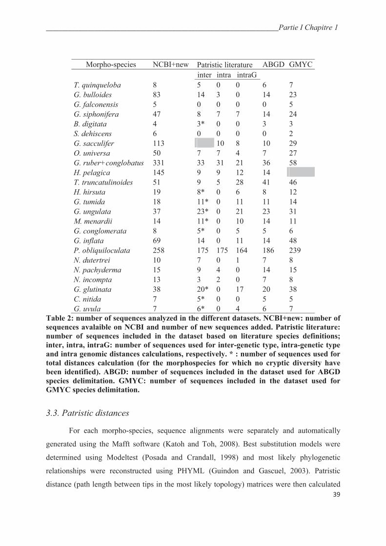
________________________________________________________________________Partie I Chapitre 1
39
Morpho-species NCBI+new Patristic literature ABGD GMYC
inter intra intraG
T. quinqueloba 8 5 0 0 6 7
G. bulloides 83 14 3 0 14 23
G. falconensis 5 0 0 0 0 5
G. siphonifera 47 8 7 7 14 24
B. digitata 4 3* 0 0 3 3
S. dehiscens 6 0 0 0 0 2
G. sacculifer 113 10 8 10 29
O. universa 50 7 7 4 7 27
G. ruber+conglobatus 331 33 31 21 36 58
H. pelagica 145 9 9 12 14
T. truncatulinoides 51 9 5 28 41 46
H. hirsuta 19 8* 0 6 8 12
G. tumida 18 11* 0 11 11 14
G. ungulata 37 23* 0 21 23 31
M. menardii 14 11* 0 10 14 11
G. conglomerata 8 5* 0 5 5 6
G. inflata 69 14 0 11 14 48
P. obliquiloculata 258 175 175 164 186 239
N. dutertrei 10 7 0 1 7 8
N. pachyderma 15 9 4 0 14 15
N. incompta 13 3 2 0 7 8
G. glutinata 38 20* 0 17 20 38
C. nitida 7 5* 0 0 5 5
G. uvula 7 6* 0 4 6 7
Table 2: number of sequences analyzed in the different datasets. NCBI+new: number of
sequences avalaible on NCBI and number of new sequences added. Patristic literature:
number of sequences included in the dataset based on literature species definitions;
inter, intra, intraG: number of sequences used for inter-genetic type, intra-genetic type
and intra genomic distances calculations, respectively. * : number of sequences used for
total distances calculation (for the morphospecies for which no cryptic diversity have
been identified). ABGD: number of sequences included in the dataset used for ABGD
species delimitation. GMYC: number of sequences included in the dataset used for
GMYC species delimitation.
3.3. Patristic distances
For each morpho-species, sequence alignments were separately and automatically
generated using the Mafft software (Katoh and Toh, 2008). Best substitution models were
determined using Modeltest (Posada and Crandall, 1998) and most likely phylogenetic
relationships were reconstructed using PHYML (Guindon and Gascuel, 2003). Patristic
distance (path length between tips in the most likely topology) matrices were then calculated
________________________________________________________________________Partie I Chapitre 1
40
using the APE package of R software (R Development Core Team, 2004; Paradis et al.,
2004). Patristic distances were preferred over pairwise distances to better account for multiple
substitutions at the same site. For some of the studied morpho-species, as for example Gs.
ruber and Gs. sacculifer, many of the available sequences were identical while for others, as
for example Turborotalia quinqueloba and Neogloboquadrina pachyderma, almost all the
deposited sequences corresponded to different haplotypes. This phenomenon is probably an
artifact reflecting the number of sequences available, the quality of sampling and/or an
arbitrary selection performed by the authors for sequences to be deposited. As a consequence,
in our calculations, we retained a single sequence per haplotype (i.e., a unique sequence per
pool of identical sequences). We calculated patristic distances within each morpho-species
and extracted distances within the defined genetic types and among individuals from different
genetic types. We also calculated intra-genomic distances for each morpho-species. Since this
calculation only requires individual and morpho-species identifications, sequences that lack
information on their genetic type in NCBI have been added to the analysis. Considering the
lack of several genotype labels in NCBI and the shortness of many sequences, it appears
finally that the dataset that have been used for calculation of patristic distance values was
reduced to less than 30% of the available sequences (Table 2). In particular, all sequences of
the Type II of Orbulina universa (de Vargas et al., 1999), and all sequences of Globoconella
inflata with identified genetic types were excluded from our analysis. In addition, cryptic
diversity has never been studied in the case of several morpho-species (e.g., Globorotalia
tumida and Globoquadrina conglomerata). For comparing intra- and inter-genetic type and
overall patristic distance distributions we used the Kolmogorov-Smirnov and Mann-Whitney
tests implemented in PAST v. 2.17c (Hammer et al., 2001)
Distances between genetic types (inter-type distances) are expected to be higher than
distances within genetic types (intra-type distances) whenever the genetic types correspond to
genuine species. In this case, inter- and intra-type distances are separated by a distance gap
(e.g., Lefébure et al., 2006, Puillandre et al., 2012a). Distances within individuals (intra-
genomic distances) should be included in the intra-type distance range. Consequently,
whenever a morpho-species displays these distance patterns, we consider here its genetic
types as most probably accurately delimitated.
________________________________________________________________________Partie I Chapitre 1
41
3.4. Automatic genetic type delimitation methods
Genetic type delimitations used for the patristic distances approach were suggested
empirically and thus rely on each author’s, potentially subjective reading and interpretation of
phylogenetic trees. To avoid this, we used the Automatic Barcode Gap Detection (ABGD;
Puillandre et al., 2012a) and General Mixed Yule Coalescent (GMYC; Pons et al., 2006)
methods as complementary approaches for species delimitation in modern planktonic
foraminifera. ABGD and GMYC newly-defined delimitations were evaluated through the
patristic distance approach; we consider as most probably accurate the delimitations that are
cross-validated with the patristic distance approach.
3.4.1 Automatic Barcode Gap Delimitation (ABGD)
ABGD is an automatic procedure that sorts sequences into putative species based on a
barcode gap, i.e., the gap in genetic distances distribution between intraspecific and
interspecific diversity (Puillandre et al., 2012a). This barcode gap is observed whenever the
divergence among organisms belonging to the same species is lower than divergence among
organisms from different species (Puillandre et al., 2012a). The ABGD method is more
efficient when the number of species is not too large and the evolutionary rate differences
between species are limited (Puillandre et al., 2012a). Consequently, given the particularly
heterogeneous rates of molecular evolution in planktonic foraminifera (de Vargas et al.,
1997), we ran ABGD for each morpho-species alignment independently, using the default
settings and the K-80 pairwise distance method (Kimura, 1980). As this method does not rely
on a prior definition of taxonomic units, the analyzed dataset includes the sequences that
lacked genetic type label.
In some cases, the ABGD method identifies several MOTUs plateaus corresponding to
decreasing number of genetic types delimitated within the dataset. First, when necessary, we
discarded the delimitation hypotheses that assigned clones from the same individual to
distinct genetic types. Among the remaining hypotheses, we considered the first MOTUs
plateau (i.e. maximum number of MOTUs) as corresponding to the putative species
delimitation (Puillandre et al., 2012a ; Laetsch et al., 2012). Indeed, this first MOTU plateau
is most likely marking the distance gap between intra-species distances (i.e., the shortest
distances within the dataset) and the distances between the closest putative species (Laetsch et
________________________________________________________________________Partie I Chapitre 1
42
al., 2012), whereas the second plateau usually reflects the distance gap between clades of
putative species.
3.4.2. General Mixed Yule Coalescent (GMYC)
The GMYC approach (Pons et al., 2006) identifies boundaries between evolutionary
units on the basis of shifts in branching rates. Branching within species is the result of
coalescent processes, whereas branching between species reflects the timing of speciation
events (Fontaneto et al., 2007). This approach is thus independent from both previous
taxonomic delimitations and genetic distances. As a consequence, all planktonic foraminiferal
sequences can be equally treated. The study of Hoef-Emden (2012) demonstrates that GMYC
can be successfully applied to multi-copy ribosomal genes. Preliminary experiments suggest
that it requires a minimum number of biological species for accurately rejecting the null
hypothesis that all sequences belong to the same species. In our analysis, given the genetic
distances encountered between planktonic foraminifera, we selected 5 subsets of sequences
(each of them including 3 to 7 morpho-species) from the phylogeny published by Aurahs et
al. (2009b) in order to avoid ambiguous alignments (Table 3): (i) the two clades within the
spinose taxa, (ii) the two clades within the macroperforate non-spinose taxa, and (iii) the
microperforate clade. Multiple species alignments were automatically generated using the
Mafft software (Katoh and Toh, 2008) and checked manually for alignment errors. A single
sequence per haplotype was retained and the best substitution model was selected using
Modeltest (Posada and Crandall, 1998) under AIC criterion (Akaike, 1974). Ultrametric trees
were generated with the BEAST software (Lemey et al., 2010) using a log-normal relaxed
molecular clock (Drummond et al., 2012) without calibration point. These trees were then
used as an input for GMYC species delimitation using the Splits package (Ezard et al., 2009)
for R software (R Development Core Team, 2004).
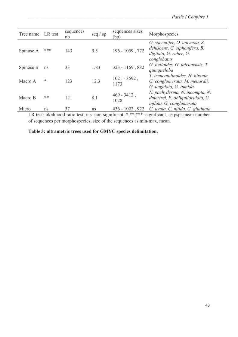
________________________________________________________________________Partie I Chapitre 1
43
Tree name LR test sequences
nb seq / sp
sequences sizes
(bp) Morphospecies
Spinose A *** 143 9.5 196 - 1059 , 772
G. sacculifer, O. universa, S.
dehiscens, G. siphonifera, B.
digitata, G. ruber, G.
conglobatus
Spinose B ns 33 1.83 323 - 1169 , 882 G. bulloides, G. falconensis, T.
quinqueloba
Macro A * 123 12.3 1021 - 3592 ,
1173
T. truncatulinoides, H. hirsuta,
G. conglomerata, M. menardii,
G. ungulata, G. tumida
Macro B ** 121 8.1 469 - 3412 ,
1028
N. pachyderma, N. incompta, N.
dutertrei, P. obliquiloculata, G.
inflata, G. conglomerata
Micro ns 37 ns 436 - 1022 , 922 G. uvula, C. nitida, G. glutinata
LR test: likelihood ratio test, n.s=non significant, *,**,***=significant. seq/sp: mean number
of sequences per morphospecies, size of the sequences as min-max, mean.
Table 3: ultrametric trees used for GMYC species delimitation.

________________________________________________________________________Partie I Chapitre 1
44
4. Results
4.1. Patristic distances
As a result of procedure requirement, inter-type and intra-type distances could be
estimated for 10 morpho-species out of 22 (Fig. 9A). Inter-type distances are highly variable
between morpho-species, ranging from 0.12 % (minimum, Turboratalia quinqueloba) to more
than 60% (maximum, Globigerinoides ruber+conglobatus and Hastigerina pelagica). Intra-
type distances are less variable than inter-type distances as they range from 0% (minimum as
nearly all species include identical sequences) to 4.5% (maximum, Truncorotalia
truncatulinoides). Overall intra-type distances are significantly lower than inter-type distances
(Table 4), implying that patristic distances can be used as a criterion for genetic type
delimitation. For 4 morpho-species (Globigerinella siphonifera, O. universa, Hastigerina
pelagica and Neogloboquadrina incompta), we observed a clear distance gap between inter-
type and intra-type distances. Distance gap is reduced in the cases of Neogloboquadrina
pachyderma and Globigerina bulloides; for 3 morpho-species (Gs. ruber+conglobatus,
Pulleniatina obliquiloculata and T. truncatulinoides), intra-type and inter-type distances
overlap. Intra-type distances could not be calculated in the case of Turborotalia quinqueloba
as all haplotypes correspond to different genetic types. Overall, intra-genomic distances could
be estimated for 17 morpho-species. They range from 0% (identical sequences) to 4.8% (T.
truncatulinoides). These distances are thus of the same range, or lower, than the intra-type
distances within the same morpho-species (Table 5). For 11 morpho-species, neither inter-
type nor intra-type distances could be estimated because none of their sequences retained for
this analysis was assigned to their genetic type. In the case of G. inflata, G. conglomerata,
Hirsutella hirsuta, Gr. tumida, Gr. ungulata, Menardella menardii and Candeina nitida, the
total genetic distances are of the same range as the intra-genomic distances estimated for these
morpho-species (Table 6). On the contrary, in the case of Globigerinita uvula and
Globigerinita glutinata, these distances are significantly higher that the intra-genomic
distances estimated for these morpho-species (Table 6).
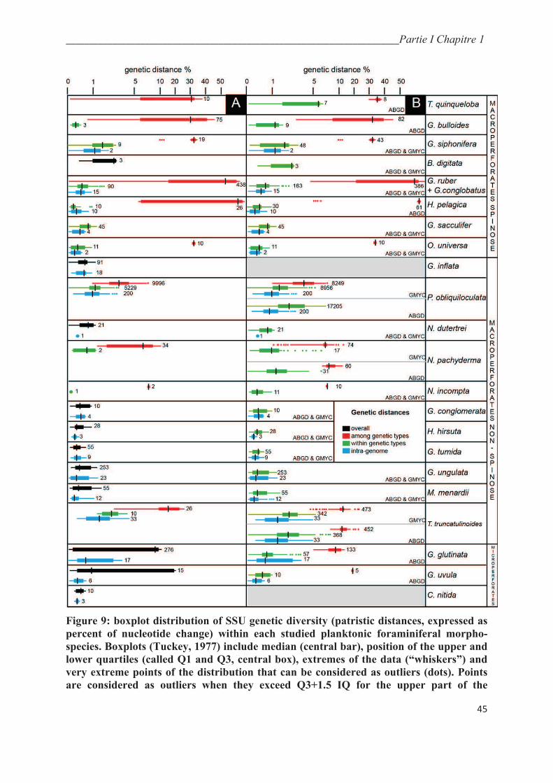
________________________________________________________________________Partie I Chapitre 1
45
Figure 9: boxplot distribution of SSU genetic diversity (patristic distances, expressed as
percent of nucleotide change) within each studied planktonic foraminiferal morpho-
species. Boxplots (Tuckey, 1977) include median (central bar), position of the upper and
lower quartiles (called Q1 and Q3, central box), extremes of the data (“whiskers”) and
very extreme points of the distribution that can be considered as outliers (dots). Points
are considered as outliers when they exceed Q3+1.5 IQ for the upper part of the
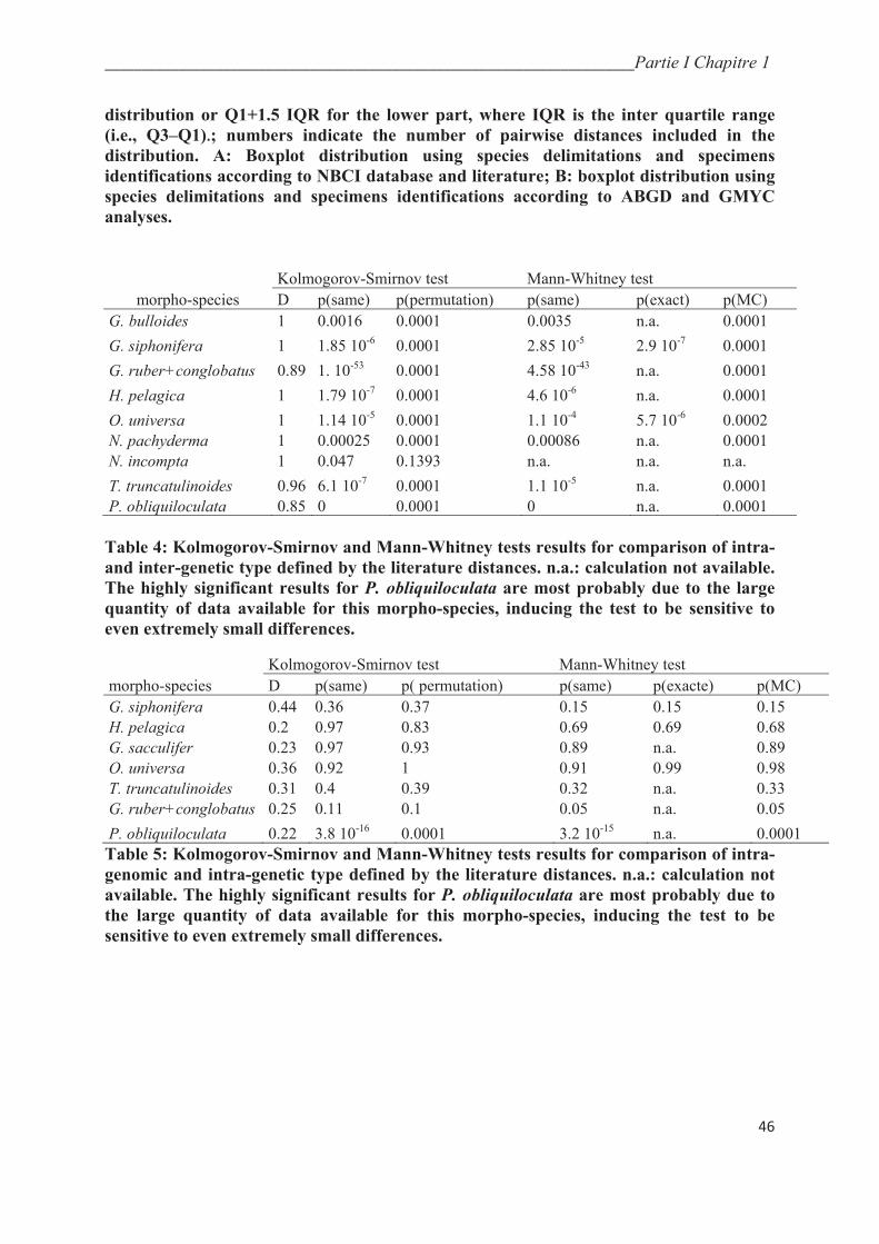
________________________________________________________________________Partie I Chapitre 1
46
distribution or Q1+1.5 IQR for the lower part, where IQR is the inter quartile range
(i.e., Q3–Q1).; numbers indicate the number of pairwise distances included in the
distribution. A: Boxplot distribution using species delimitations and specimens
identifications according to NBCI database and literature; B: boxplot distribution using
species delimitations and specimens identifications according to ABGD and GMYC
analyses.
Kolmogorov-Smirnov test Mann-Whitney test
morpho-species D p(same) p(permutation) p(same) p(exact) p(MC)
G. bulloides 1 0.0016 0.0001 0.0035 n.a. 0.0001
G. siphonifera 1 1.85 10-6 0.0001 2.85 10-5 2.9 10-7 0.0001
G. ruber+conglobatus 0.89 1. 10-53 0.0001 4.58 10-43 n.a. 0.0001
H. pelagica 1 1.79 10-7 0.0001 4.6 10-6 n.a. 0.0001
O. universa 1 1.14 10-5 0.0001 1.1 10-4 5.7 10-6 0.0002
N. pachyderma 1 0.00025 0.0001 0.00086 n.a. 0.0001
N. incompta 1 0.047 0.1393 n.a. n.a. n.a.
T. truncatulinoides 0.96 6.1 10-7 0.0001 1.1 10-5 n.a. 0.0001
P. obliquiloculata 0.85 0 0.0001 0 n.a. 0.0001
Table 4: Kolmogorov-Smirnov and Mann-Whitney tests results for comparison of intra-
and inter-genetic type defined by the literature distances. n.a.: calculation not available.
The highly significant results for P. obliquiloculata are most probably due to the large
quantity of data available for this morpho-species, inducing the test to be sensitive to
even extremely small differences.
Kolmogorov-Smirnov test Mann-Whitney test
morpho-species D p(same) p( permutation) p(same) p(exacte) p(MC)
G. siphonifera 0.44 0.36 0.37 0.15 0.15 0.15
H. pelagica 0.2 0.97 0.83 0.69 0.69 0.68
G. sacculifer 0.23 0.97 0.93 0.89 n.a. 0.89
O. universa 0.36 0.92 1 0.91 0.99 0.98
T. truncatulinoides 0.31 0.4 0.39 0.32 n.a. 0.33
G. ruber+conglobatus 0.25 0.11 0.1 0.05 n.a. 0.05
P. obliquiloculata 0.22 3.8 10-16 0.0001 3.2 10-15 n.a. 0.0001
Table 5: Kolmogorov-Smirnov and Mann-Whitney tests results for comparison of intra-
genomic and intra-genetic type defined by the literature distances. n.a.: calculation not
available. The highly significant results for P. obliquiloculata are most probably due to
the large quantity of data available for this morpho-species, inducing the test to be
sensitive to even extremely small differences.

________________________________________________________________________Partie I Chapitre 1
47
Kolmogorov-Smirnov test Mann-Whitney test
morpho-species D p(same) p(permutation) p(same) pexact p(MC)
G. conglomerata 0.4 0.47 0.42 0.2 0.23 0.23
H. hirsuta 0.71 0.16 0.31 0.29 0.34 0.35
G. ungulata 0.37 0.004 0.06 0.11 n.a. 0.12
G. tumida 0.29 0.4 0.43 0.29 n.a. 0.29
M. menardii 0.37 0.17 0.26 0.28 n.a. 0.28
G. inflata 0.22 0.45 0.4 0.9 n.a. 0.9
C. nitida 0.5 0.45 0.27 0.3 n.a. 0.29
G. uvula 0.6 0.05 0.055 0.039 0.034 0.04
G. glutinata 0.7 10^-5 0.0001 10^-4 n.a. 0.0001
Table 6: Kolmogorov-Smirnov and Mann-Whitney tests results for comparison of intra-
genomic and overall distances for morpho-species without genetic type defined by the
literature. n.a.: calculation not available.
4.2. Automatic genetic type delimitation methods
4.2.1 ABGD
No barcoding gap was identified for 7 morpho-species (Globigerinoides sacculifer,
Beela digitata, Globorotalia tumida, Hirsutella hirsuta, Neogloboquadrina dutertrei,
Pulleniatina obliquiloculata and Globoconella inflata). Consequently, according to this
method, these morpho-species should correspond to single genuine species (Table 7). In the
case of Gc. inflata, because of their short length, none of the initial sequences used to
characterize the two identified genetic types (Morard et al., 2011) have been analyzed.
Consequently, we cannot exclude that our dataset contains only sequences from one of the
two types identified by Morard et al. (2011). For 6 morpho-species (Orbulina universa,
Turborotalia quinqueloba, Truncorotalia truncatulinoides, Neogloboquadrina pachyderma,
Neogloboquadrina incompta, and Globigerinita uvula) the ABGD method identifies only one
species delimitation optimum (i.e., one MOTUs richness plateau). For the remaining 8
morpho-species, it identifies several species delimitations optima. Due to miss-assignment of
clones, we retained the one-MOTU delimitation for Globorotalia ungulata, Menardella
menardii and Globoquadrina conglomerata, and the four-MOTU delimitation for
Globigerinita glutinata. For the remaining 4 morpho-species we considered the first MOTUs
plateau for putative species delimitation. Consequently, 7 putative species within Globigerina
bulloides, 5 putative species within Globigerinodes ruber+conglobatus, and 3 putative
species within Globigerinella siphonifera and Hastigerina pelagica were retained.
Finally, ABGD putative species delimitations are similar to previously defined genetic
types for 5 morpho-species: O. universa, Gs. sacculifer, Ge. siphonifera, H. pelagica and N.
________________________________________________________________________Partie I Chapitre 1
48
incompta (Table 7). This method lumps some of the previously defined genetic types into the
same species for 7 morpho-species: T. quinqueloba, Gg. bulloides, Gs. ruber+conglobatus, N.
pachyderma, P. obliquiloculata, Gc. inflata and T. truncatulinoides. Putative species
delimitations were obtained for the first time for 9 morpho-species: B. digitata, N. dutertrei,
Gr. tumida, Ht. hirsuta, Gr. ungulata, Gr. menardii, Gq. conglomerata, Ga. glutinata and G.
uvula.
We calculated patristic distances among and within putative species as they are
defined by the ABGD method. As expected for a distance-based method (Puillandre et al.,
2012a), patristic distances are compatible with the ABGD delimitations (Fig. 9B), except for
T. truncatulinoides, which still exhibits a slight overlap between intra-genetic types and inter-
genetic types (Fig. 9B).

________________________________________________________________________Partie I Chapitre 1
49
morphospecies literature patristic ABGD GMYC
T. quinqueloba
Ia
invalidated (1)
I
T. quinqueloba*
Ib
IIa
II IIb
IIc
IId
G. bulloides
Ia
invalidated (1)
Ia
G. bulloides*
Ib
Ib-c-e Ic
Ie
Id Id
IIa IIa
IIb
IIb-d-f IId
IIf
IIe IIe
IIc IIc
B. digitata n. d. B. digitata B. digitata B. digitata
S. dehiscens n. d. n. a. n. a. S. dehiscens
G. siphonifera
I
validated
I I
IIa=II II II
IIb=III III III
G. ruber +
conglobatus
G.
conglobatus
invalidated (2)
G. conglobatus G. conglobatus
IIa
IIa IIa IIa1
IIa2
IIb n. a. IIb
Ia Ia Ia
Ib1 Ib Ib
Ib2
pink pink pink
G. sacculifer G. sacculifer validated G. sacculifer G. sacculifer
O. universa
II n. a. n. a. II
I
validated
I I
III III
IIIa
n. a. n. a. IIIb
H. pelagica
I
validated
I
n. a. IIa IIa
IIb IIb
= III
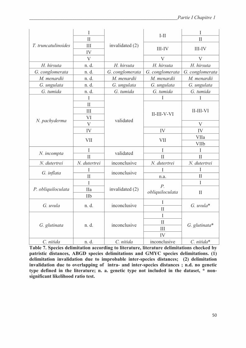
________________________________________________________________________Partie I Chapitre 1
50
T. truncatulinoides
I
invalidated (2)
I-II I
II II
III III-IV III-IV
IV
V V V
H. hirsuta n. d. H. hirsuta H. hirsuta H. hirsuta
G. conglomerata n. d. G. conglomerata G. conglomerata G. conglomerata
M. menardii n. d. M. menardii M. menardii M. menardii
G. ungulata n. d. G. ungulata G. ungulata G. ungulata
G. tumida n. d. G. tumida G. tumida G. tumida
N. pachyderma
I
validated
I I
II
II-III-V-VI II-III-VI III
VI
V V
IV IV IV
VII VII VIIa
VIIb
N. incompta I
validated I I
II II II
N. dutertrei N. dutertrei inconclusive N. dutertrei N. dutertrei
G. inflata I
inconclusive I I
II n.a. II
P. obliquiloculata
I
invalidated (2) P.
obliquiloculata
I
IIa II
IIb
G. uvula n. d. inconclusive I
G. uvula* II
G. glutinata n. d. inconclusive
I
G. glutinata* II
III
IV
C. nitida n. d. C. nitida inconclusive C. nitida*
Table 7. Species delimitation according to literature, literature delimitations checked by
patristic distances, ABGD species delimitations and GMYC species delimitations. (1)
delimitation invalidation due to improbable inter-species distances; (2) delimitation
invalidation due to overlapping of intra- and inter-species distances ; n.d. no genetic
type defined in the literature; n. a. genetic type not included in the dataset, * non-
significant likelihood ratio test.
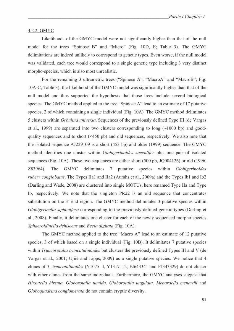
________________________________________________________________________Partie I Chapitre 1
51
4.2.2. GMYC
Likelihoods of the GMYC model were not significantly higher than that of the null
model for the trees “Spinose B” and “Micro” (Fig. 10D, E; Table 3). The GMYC
delimitations are indeed unlikely to correspond to genetic types. Even worse, if the null model
was validated, each tree would correspond to a single genetic type including 3 very distinct
morpho-species, which is also most unrealistic.
For the remaining 3 ultrametric trees (“Spinose A”, “MacroA” and “MacroB”; Fig.
10A-C; Table 3), the likelihood of the GMYC model was significantly higher than that of the
null model and thus supported the hypothesis that those trees include several biological
species. The GMYC method applied to the tree “Spinose A” lead to an estimate of 17 putative
species, 2 of which containing a single individual (Fig. 10A). The GMYC method delimitates
5 clusters within Orbulina universa. Sequences of the previously defined Type III (de Vargas
et al., 1999) are separated into two clusters corresponding to long (~1000 bp) and good-
quality sequences and to short (<450 pb) and old sequences, respectively. We also note that
the isolated sequence AJ229109 is a short (453 bp) and older (1999) sequence. The GMYC
method identifies one cluster within Globigerinoides sacculifer plus one pair of isolated
sequences (Fig. 10A). These two sequences are either short (500 pb, JQ004126) or old (1996,
Z83964). The GMYC delimitates 7 putative species within Globigerinoides
ruber+conglobatus. The Types IIa1 and IIa2 (Aurahs et al., 2009a) and the Types Ib1 and Ib2
(Darling and Wade, 2008) are clustered into single MOTUs, here renamed Type IIa and Type
Ib, respectively. We note that the singleton PR22 is an old sequence that concentrates
substitution on the 3’ end region. The GMYC method delimitates 3 putative species within
Globigerinella siphonifera corresponding to the previously defined genetic types (Darling et
al., 2008). Finally, it delimitates one cluster for each of the newly sequenced morpho-species
Sphaeroidinella dehiscens and Beela digitata (Fig. 10A).
The GMYC method applied to the tree “Macro A” lead to an estimate of 12 putative
species, 3 of which based on a single individual (Fig. 10B). It delimitates 7 putative species
within Truncorotalia truncatulinoides but clusters the previously defined Types III and V (de
Vargas et al., 2001; Ujiié and Lipps, 2009) as a single putative species. We notice that 4
clones of T. truncatulinoides (Y1075_4, Y1317_12, FJ643341 and FJ343329) do not cluster
with other clones from the same individuals. Furthermore, the GMYC analyses suggest that
Hirsutella hirsuta, Globorotalia tumida, Globorotalia ungulata, Menardella menardii and
Globoquadrina conglomerata do not contain cryptic diversity.
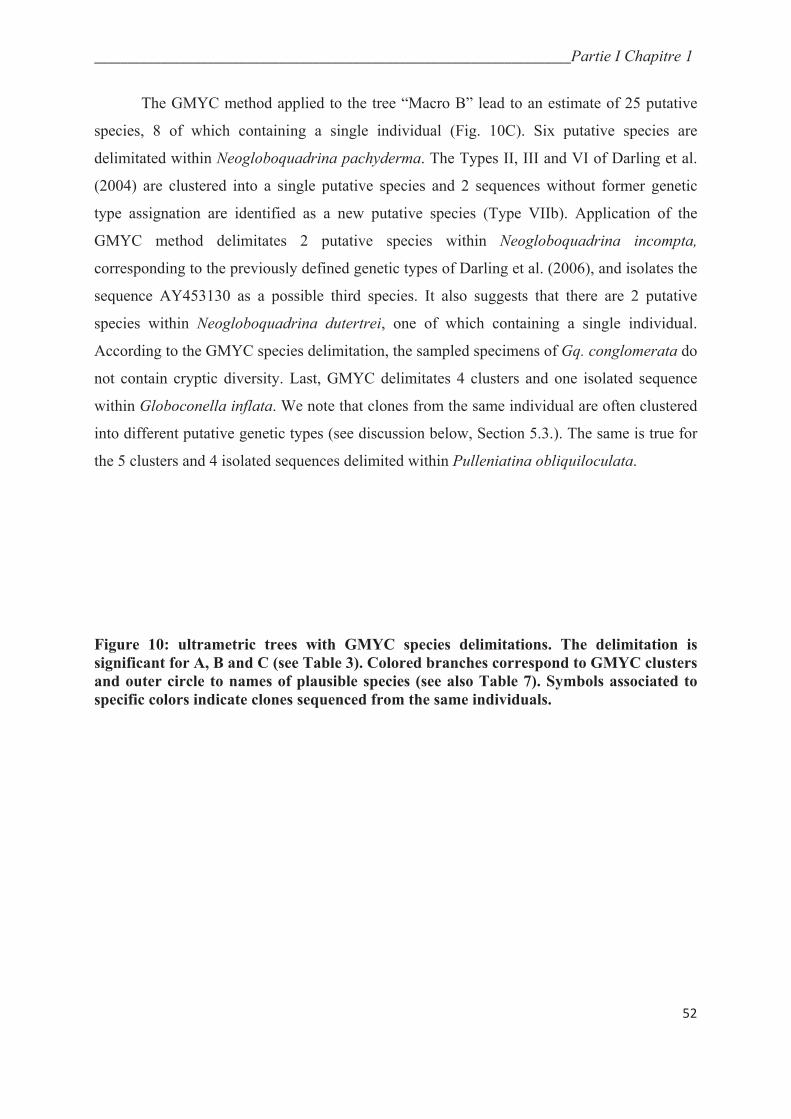
________________________________________________________________________Partie I Chapitre 1
52
The GMYC method applied to the tree “Macro B” lead to an estimate of 25 putative
species, 8 of which containing a single individual (Fig. 10C). Six putative species are
delimitated within Neogloboquadrina pachyderma. The Types II, III and VI of Darling et al.
(2004) are clustered into a single putative species and 2 sequences without former genetic
type assignation are identified as a new putative species (Type VIIb). Application of the
GMYC method delimitates 2 putative species within Neogloboquadrina incompta,
corresponding to the previously defined genetic types of Darling et al. (2006), and isolates the
sequence AY453130 as a possible third species. It also suggests that there are 2 putative
species within Neogloboquadrina dutertrei, one of which containing a single individual.
According to the GMYC species delimitation, the sampled specimens of Gq. conglomerata do
not contain cryptic diversity. Last, GMYC delimitates 4 clusters and one isolated sequence
within Globoconella inflata. We note that clones from the same individual are often clustered
into different putative genetic types (see discussion below, Section 5.3.). The same is true for
the 5 clusters and 4 isolated sequences delimited within Pulleniatina obliquiloculata.
Figure 10: ultrametric trees with GMYC species delimitations. The delimitation is
significant for A, B and C (see Table 3). Colored branches correspond to GMYC clusters
and outer circle to names of plausible species (see also Table 7). Symbols associated to
specific colors indicate clones sequenced from the same individuals.
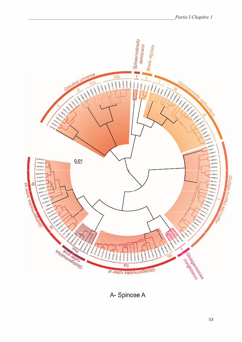
____________________________________________________________Partie I Chapitre 1
53
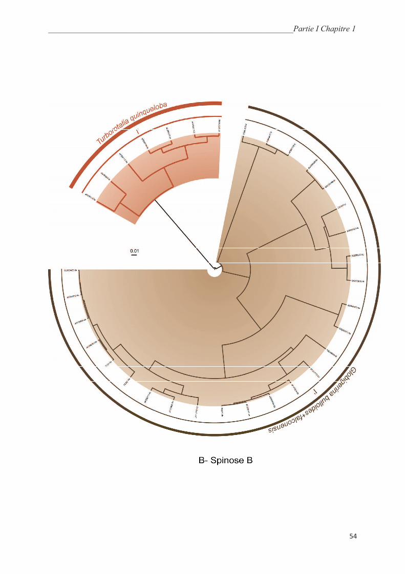
____________________________________________________________Partie I Chapitre 1
54
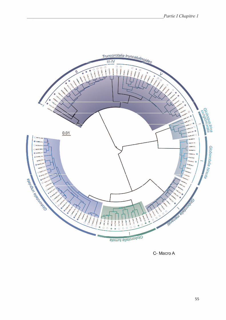
____________________________________________________________Partie I Chapitre 1
55

____________________________________________________________Partie I Chapitre 1
56
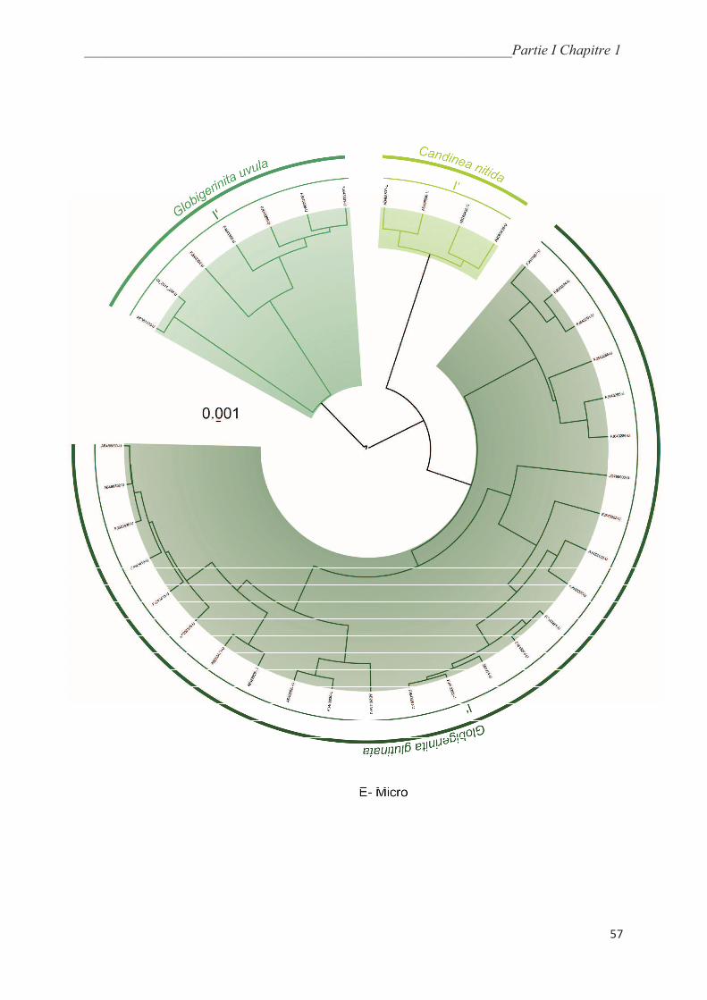
____________________________________________________________Partie I Chapitre 1
57
________________________________________________________________________Partie I Chapitre 1
58
5. Discussion
5.1. Heterogeneity of previous genetic type delimitations
According to patristic distance analyses, previous genetic type delimitations
correspond to genuine cryptic species in only 4 morpho-species (Globigerinella siphonifera,
Orbulina universa, Hastigerina pelagica and Neogloboquadrina incompta; Table 7). Because
Globigerinoides sacculifer overall and intra-genomic distances are within the same range, the
absence of cryptic diversity within this morpho-species (André et al., 2013) is validated. The
case of Neogloboquadrina pachyderma remains potentially ambiguous, as intra-specific and
inter-specific distances are separated by virtually no distance gap (0.09 %). Within
Globigerina bulloides, the distance gap is also reduced (0.4 %) and the diversity between
some of the previously defined genetic types is very low (0.9 %). It corresponds to intra-type
distances in other morpho-species (Fig. 9A), suggesting that this morpho-species may have
been oversplit. The same apply to Turborotalia quinqueloba for which the difference between
some of the previously defined genetic types is extremely low (0.12%). Likewise, the overlap
between intra-type and inter-type distances in Globigerinoides ruber+conglobatus and
Pulleniatina obliquiloculata shows that at least some of the previously defined genetic types
within these morpho-species may not correspond to genuine species. Results suggest that
Globoconella inflata, Globoquadrina conglomerata, Hirsutella hirsuta, Globorotalia tumida,
Globorotalia ungulata, Menardella menardii and Candeina nitida do not hide cryptic
diversity given their reduced overall patristic distances. Overall distances within
Neogloboquadrina dutertrei and Beela digitata seem to match intra-type distances but data
are too scarce to draw firm conclusions. Genetic distances within Globigerinita uvula and
Globigerinita glutinata are particularly high and clearly out of range of intra-type distances,
suggesting that both these morpho-species may constitute complexes of yet unknown cryptic
species. The case of these species points to a major drawback of the patristic distance
approach: it requires a-priori genetic type delimitations.
Our study shows that the empirical delimitations available in the literature suffer from
subjectivity and are thus not homogenous: some previously-defined genetic types are likely to
correspond to valid taxonomic units whereas others probably represent sub-species or
population level structuration. Among the morpho-species for which genetic type delimitation
seems accurate, intra-specific distances are quite variable as well as the range of the distance
________________________________________________________________________Partie I Chapitre 1
59
gap between intra-specific and inter-specific distances (Fig. 9). This phenomenon may be the
result of the heterogeneity of substitution rates observed between planktonic foraminiferal
lineages and even sometimes between more closely related morpho-species (de Vargas et al.,
1997). Consequently, we hypothesize that the design of a unique threshold value between
intra-specific and inter-specific distances would not be appropriate in the case of planktonic
foraminifera.
5.2. ABGD: an efficient method to build species delimitation hypotheses in
planktonic foraminifera
As expected for a distance-based method, delimitations resulting from ABGD are
validated through the patristic distance approach (Fig. 9, Table 7). However,
Neogloboquadrina pachyderma and Truncorotalia truncatulinoides constitute two exceptions.
In N. pachyderma, ABGD favors an alternative genetic type delimitation (Table 7) that is
clearly cross-validated by the patristic distances approach. Although the gap between intra-
type and inter-type distances was extremely reduced, published genetic types are also
validated and we consequently cannot determine which delimitation (i.e., literature or ABGD)
should be favored. In T. truncatulinoides, delimitation resulting from ABGD is not cross-
validated through the patristic distances approach. Nevertheless, the overlap between intra-
type and inter-type distances is much reduced using the ABGD delimitation compared to the
literature-based delimitation (Fig. 9).
We also calculated patristic distances for the genetic type delimitations corresponding
to the second MOTUs plateaus generated by ABGD in the cases of Globigerinella siphonifera
Hastigerina pelagica, Globigerina bulloides and Globigerinoides ruber+conglobatus
(supplementary data 2). We obtained high intra-specific distances (up to 10%) corresponding
to 4 to 8 times the intra-genomic distances. Consequently, these alternative species
delimitations appear to be less likely and the first MOTUs plateau is comforted as the optimal
genetic type delimitation.
Finally, even if the ABGD and patristic distances approaches are highly congruent,
calculation of patristic distances is still of interest as it comforts genuine species delimitations
by screening unrealistic hypotheses. Running ABGD is fast enough and efficient for building
species delimitation hypotheses, even when only a few sequences are available, as for
example in Globigerinita uvula. Consequently, this method should be intended first for

________________________________________________________________________Partie I Chapitre 1
60
planktonic foraminiferal species delimitation hypotheses. Importantly, a current limit to this
method is the requirement that the alignment is void of missing data. A direct consequence is
the exclusion of potential cryptic species from analyses (for example the Types II and IIIb of
Orbulina universa, the Type IIb of Globigerinoides ruber and the Type II of Globoconella
inflata). Thus, the generalized use of ABGD for planktonic foraminiferal species delimitation
would require a standardization of the sequenced and deposited SSU regions.
5.3. GMYC: a distance-independent method for building species delimitations in
planktonic foraminifera
The GMYC method isolates numerous divergent haplotypes as putative species (Fig.
10). All of these sequences in Orbulina universa (AJ229109), Globigerinoides ruber
(Z839665) and Globigerinoides sacculifer (JQ004126 and Z83964), correspond to old
(submitted to the NCBI database back in 1996) or short sequences (~500 bp). Furthermore,
they concentrate substitutions on the 5’ end region. We speculate that the apparent divergence
of these sequences is thus likely to be the result of PCR and/or sequencing artifacts that were
more frequent with older amplification and sequencing chemistry. Consequently, we do not
retain these sequences as genuine species. Furthermore, patristic distances between these
divergent haplotypes within Gs. ruber and G. sacculifer and the other sequences from their
closest putative species were clearly of intra-type distance range, confirming that the
corresponding sequences should not be considered as separate species (supplementary data 2).
GMYC classification of the sequences of the Type III of O. universa into two putative species
is also a likely artifact as it only reflects differences in length and quality of the sequences. As
a conclusion, after close examination on the GMYC results, the number of putative species
delimitated by the GMYC method is reduced to 3 within O. universa, 6 within Gs.
ruber+conglobatus, and 1 within Gs. sacculifer (Table 7).
The GMYC method also assigned SSU copies from the same individuals to different
putative species. This assignment may be the result of 3 phenomena: (i) non-concerted
evolution between copies within the genome (Mayol and Rosello, 2001); (ii) when genetic
distances are low, PCR and/or sequencing errors can produce enough noise obliterating the
true phylogenetic signal (Maddison and Knowles, 2006); and (iii) horizontal gene transfer, a
rare phenomenon in eukaryotes taxa that has never been evidenced for rDNA (Andersson,
________________________________________________________________________Partie I Chapitre 1
61
2005). Consequently we chose to assign clones from the same individuals to the same putative
species. The number of putative species within Truncorotalia truncatulinoides is thus reduced
to 4 (Fig. 10B). Likewise, diversities in Globoconella inflata and Pulleniatina obliquiloculata
are reduced to 2 putative species. Genetic diversity within Gc. inflata was mostly studied on
the fast-evolving ITS genes because SSU divergence is particularly low (Morard et al., 2011).
Consequently, a few PCR and/or sequencing artifacts might have induced the assignment of
clones to different putative species. As the intra-genomic diversity is extensive within P.
obliquiloculata, we speculate that non-concerted evolution of SSU rDNA copies within
genomes may have generated the widespread sorting of clones from the same individuals into
different clusters observed for this morpho-species.
Together, GMYC delimitations corroborate all previous genetic type delimitations
supported as genuine species using the patristic distance approach, with the exception of
Neogloboquadrina pachyderma (Table 7). Importantly, the taxonomic status of previously
described genetic types of N. pachyderma was slightly ambiguous according to patristic
distances. The new putative species delimitations obtained through the GMYC method were
tested with the patristic distance approach. For all morpho-species but T. truncatulinoides, N.
pachyderma and P. obliquiloculata, these new delimitations are supported as genuine species
by the patristic approach as we observed a clear distance gap between intra-type and inter-
type distances, or, in the case of the morpho-species without cryptic diversity, plausible intra-
specific distance ranges (Fig. 9). Still, we were not able to cross-check the species status of
the Type II and IIIb of O. universa (Fig. 10A) and the isolated sequence AJ229109, as well as
that of the Type II of Gc. inflata, the sequence AY241708 of Neogloboquadrina dutertrei, and
the sequence JQ004126 of Gs. sacculifer. In the case of N. pachyderma, P. obliquiloculata
and T. truncatulinoides, GMYC-delimitated and genetic types defined in the literature both
lead to overlap between intra- and inter-type patristic distances (Fig. 9). For T.
truncatulinoides we note that the overlap between intra-type and inter-type distances is
reduced compared to the patristic approach based on previous genetic type delimitations. The
topology of the N. pachyderma tree is highly sensitive to model and/or method changes,
probably because only one sequence is available for 5 out of the 7 genetic types defined by
Darling et al. (2004). Given that N. pachyderma phylogram (PHYML) and ultrametric tree
(BEAST) recover quite different relationships (supplementary data 2), patristic distances were
not pertinent for testing GMYC delimitations. Last, even after close examination of the

________________________________________________________________________Partie I Chapitre 1
62
dataset of P. obliquiloculata, we were not able to infer possible artifact that might explain
why species delimitation is unsatisfactory within this morpho-species.
Our study shows that GMYC is an efficient genetic distance-independent method for
planktonic foraminiferal species delimitation using SSU rDNA sequences. However, results
also demonstrate that delimitations can be heavily impacted by data quality and thus requires
thorough inspection. Because the sequence overlap/missing data criteria are less critical than
in distance-based methods, the GMYC analysis includes more putative species than ABGD
and patristic distances analyses (Table 7, Fig. 10). Still, as GMYC is a time-consuming
method, it should not be used in a first approach but rather as a cross-checking method. While
GMYC proves useful, we also recover very doubtful results where the GMYC model could
not be favored over the null model of a single coalescent population (i.e., trees “Spinose B”
and “Microperforates”; Fig. 10D, E, Table 3 and supplementary data 2). Comparison of these
cases provides guidelines on how to design sequence datasets for GMYC analysis. We notice
that the statistically significant GMYC species delimitations tend to be associated with: (i)
large datasets involving more than 2 morpho-species; (ii) datasets with few ambiguously
aligned regions, i.e. datasets including closely related morpho-species; and (iii) datasets with
overall homogenous sequence length. Indeed, the reduced size of the dataset might explain
failure to reject the null model for “Spinose B” and “Microperforates” species delimitations
and calls for more sequences from a larger set of morpho-species. In the case of the tree
“Spinose B”, integration of the divergent morpho-species Turborotalia quinqueloba might
also be at stake in putative species delimitation failure. Finally, the GMYC-delimitated
clusters within the Type III of O. universa (Fig. 10A), which apparently does not correspond
to a genuine species, show that sequence length heterogeneity may strongly influence GMYC-
based species delimitation.
5.4. Towards a molecular taxonomy of planktonic foraminifera
Patristic distance analyses show that only 6 out of the 12 morpho-species in which
cryptic diversity was evidenced on more or less empirical grounds have their putative species
correctly delimited (Table 7). The ABGD and GMYC methods gave the opportunity to cross-
check validated delimitations, and to establish new hypotheses for invalidated cases. Overall,
whatever the method used, our results clearly show that about half of the genetic types
identified in the literature are unlikely to represent genuine biological species (Table 7).

________________________________________________________________________Partie I Chapitre 1
63
Whereas the ABGD and GMYC putative species delimitation methods are
independent, their results appear highly congruent: within the SSU rDNA sequences
considered by both approaches, the ABGD method delimitates 29 genetic types, 25 (86%) of
which being identical to those defined on the basis of the GMYC method (Table 7). Among
putative species, those identically and independently defined by both methods are most
probably genuine cryptic or pseudo-cryptic biological species. The high congruence between
the two methods clearly suggests that the genetic types delimitated using a single approach
are plausible hypotheses. Our data confirm that GMYC, when compared to distance methods,
has a tendency towards over-splitting groups (Puillandre et al., 2012b ; Miralles and Vince,
2013), whereas ABGD tends to over-lump previously defined or GMYC-defined genetic
types (e.g., N. pachyderma in Table 7).
Finally, putative species delimitations remain ambiguous only for N. pachyderma, T.
truncatulinoides and P. obliquiloculata. In the case of N. pachyderma, GMYC delimitations
are clearly invalidated as genuine species through the patristic distance approach but ABGD
and literature delimitations are both possible (Fig. 9). All delimitation hypotheses for T.
truncatulinoides are invalidated through the patristic distance approach. Exploring cryptic
genetic diversity in T. truncatulinoides suffers for a lack of molecular homogeneity, since the
Types I, II, III and IV have been characterized based on ITS sequences (de Vargas et al.,
2001), whereas the Type V was characterized based on SSU sequences (Ujiié and Lipps,
2009). Only one SSU sequence has been deposited in NCBI for the Types I, III and IV of T.
truncatulinoides and the resolving power of the GYMC and ABGD methods for species
delimitation is therefore reduced (Puillandre et al., 2012a). In particular, ABGD and GMYC
disagree on the taxonomic status of the closely related Types I and II (Table 7). Using ITS
sequences, de Vargas et al. (2001) suggested genetic isolation between these two genetic
types that may be explained by a recent (100 to 200 kyrs) speciation event. Consequently,
conflicting species delimitations between ABGD and GMYC methods may be an opportunity
to detect recent speciation events that should be investigated using the ITS marker. Literature
and GMYC genetic type delimitations for P. obliquiloculata are clearly invalidated as genuine
species through the patristic distance approach. Although application of ABGD lumps all the
available sequences into a single MOTU, its specific status is still not clearly confirmed on
the basis of patristic distance values. Distance values within P. obliquiloculata are high (up to
7.6%) and, if compared with intra-genetic type distances calculated within the other morpho-
________________________________________________________________________Partie I Chapitre 1
64
species, may correspond to both intra-type and inter-type distances (Fig. 9B). Nevertheless,
these overall distance values represent only twice the intra-genomic distances which are also
particularly high (up to 3.3%), supporting then the hypothesis that this morphospecies do not
hide cryptic diversity. The lack of barcode gap within P. obliquiloculata either suggests that
the potential speciation events, if any, have occurred very recently (Pons et al., 2006;
Puillandre et al., 2012a) and/or that the high intra-genomic diversity have erased the
barcoding gap. Likewise, heterogeneous evolutionary rates between P. obliquiloculata genetic
types may generate similar values for intra-genetic type distances within fast evolving types
and for inter-genetic type distances.
5.5. Integrative taxonomy and biogeography of planktonic foraminiferal cryptic
species
The new or confirmed cryptic species delimitations discussed above are based on
molecular data which have their own limitats, in particular when dealing with closely-related
and young species (de Queiroz, 2007). Below, in an attempt to review the species status of
modern planktonic foraminifera based on an integrative taxonomy (Dayrat, 2005), we compile
our data with previously published non-molecular evidences, mostly including ecological
and/or morphological differentiations occurring among putative cryptic species.
5.5.1 Macroperforate spinoses
Patristic distances and ABGD analyses agree on the species status of the previously
defined genetic Types I, IIa and IIb of Hastigerina pelagica (Aurahs et al., 2009b; Weiner et
al., 2012). These cryptic species, collected so far in the North Atlantic, Mediterranean and
NW Pacific (Fig. 11; de Vargas et al., 1997, Ujiié and Lipps, 2009; Weiner et al., 2012),
exhibit apparently cosmopolitan sympatric distributions in temperate to tropical water masses.
Their taxonomic status is reinforced by the evidence of depth-related specializations in Types
IIa and IIb (Weiner et al., 2012). The GMYC method could not be applied to H. pelagica,
since its SSU rDNA sequences are highly divergent, leading to highly ambiguous alignments
when compared with other spinose morpho-species.
Within Turborotalia quinqueloba, SSU rDNA studies have identified six genetic types
(Darling and Wade, 2008) but the application of the ABGD method lumps these genetic types
into two cryptic species whose patristic distances are compatible with this status (Fig. 9B).
________________________________________________________________________Partie I Chapitre 1
65
These species match the two main ecological groups evidenced by Darling and Wade (2008).
The first species, here named Type I (Table 7), has been collected in Coral and Arabian Seas
(Fig. 11), and seems to be associated with warm waters of the (sub)tropical Indian and Pacific
Oceans. The second species, here named Type II (Table 7), exhibits a bipolar distribution in
cooler (sub)polar and transitional waters of both Hemispheres (Fig. 11; Darling et al., 2003).
Parker (1962) reported that at polar latitudes, surface sediment samples of Tb. quinqueloba
yield larger individuals than at lower latitudes. This author also noticed that specimens of Tb.
quinqueloba exhibit more spiny tests with latitude in the North Pacific. We speculate that
there could be a relationship between these observed morphological changes that appear to
follow water masses and the patchy distribution of the Types I and II of Tb. quinqueloba.
Application of the ABGD method lumps the eleven previously identified genetic types
of Globigerina bulloides (Darling and Wade, 2008; Morard et al., 2013; Kurasawa et al.,
unpublished) into seven species whose patristic distances are compatible with this status (Fig.
9B). The newly defined Type IIb-d-f (Table 7) lumps sequences of individuals that apparently
share similar ecology in transitional to sub-polar water masses of both hemispheres (Darling
et al., 2007; Kurasawa et al., unpublished), then making Type IIb-d-f a cosmopolitan species
with a bipolar distribution (Fig. 11). Sequences of Types Ic and Ie (Kurasawa et al.,
unpublished) from the Pacific Ocean cluster with the Type Ib sequence from the Atlantic
Ocean, suggesting that Type Ib-c-e is also a cosmopolitan species. Unfortunately, since the
exact sampling locations of Types Ic and Ie are not available, the ecological affinities of this
species remain unknown. Data is still insufficient to evidence biogeographical or ecological
differentiations between the Indo-pacific tropical Types Ia and Id. Types IIa, IIc and IIe from
colder water masses also correspond to cryptic species. Type IIe is apparently restricted to the
North Pacific (Darling and Wade, 2008). Darling et al. (2003) evidenced different timings of
reproduction which may explain genetic isolation (Norris, 2000) of the otherwise sympatric
Types IIa and IIb-d-f. Still, an integrative taxonomy for Gg. bulloides genetic types is limited
because of the scarcity of the SSU rDNA data. For example, environmental data and sampling
through different seasons are insufficient to detect potential ecological differences between
the apparently sympatric Types IIc, Type IIb-d-f and Type IIa.
Our data show that only one single species of Beela digitata has been sampled so far.
On the other hand, the distribution patterns of this rare morpho-species (Hemleben et al.,
1989) cannot be discussed in this paper, since the studied sequences originate from specimens
collected at two stations only, both located in the South Pacific (Fig. 11).
________________________________________________________________________Partie I Chapitre 1
66
All methods agree on the species status of the previously defined genetic Types I, II
and III of Globigerinella siphonifera (Darling et al., 1997; Huber et al., 1997; de Vargas et al.,
2002). Although the three cryptic species exhibit wide biogeographic distributions in the
world ocean, their observed distribution pattern suggests ecological differences that seem to
be related to nutrient availability of water masses (Fig. 11; de Vargas et al., 2002). The
biogeographic distribution and the 18
O, 13
C and Mg/Ca values of the Type I suggest that
this species is a surface-dweller from low nutrient water masses of the Indian, Pacific and
Atlantic Oceans (Huber et al., 1997; de Vargas et al., 2002). The cosmopolitan Type II has
been collected in tropical to transitional water masses of the world ocean. This species may
have a deeper depth habitat than the other cryptic species, since laboratory culture and
collections in the Ocean suggest that it could favor the deep chlorophyll maximum layers of
the water column (Huber et al., 1997; Bijma et al., 1998; de Vargas et al., 2002). Finally, the
Type III species is also a surface-dweller, but it is apparently associated with highly
productive transitional water masses and upwelling systems (de Vargas et al., 2002). Species
of Ge. siphonifera may be pseudo-cryptic, since Huber et al. (1997) evidenced clear
differences in shell porosity between Type I and Type II specimens collected from the
Caribbean.
All methods converge on the species status of the previously defined Caribbean,
Sargasso and Mediterranean genetic types of Orbulina universa (de Vargas et al., 1999),
respectively re-designated as Types I, II and III by de Vargas et al. (2004). The ABGD
method clearly delimitates the Types I and III as independent species, while sequences of the
Type II were too short to be included in the ABGD dataset. The species status of the Type II
is however supported on the basis of the GMYC method. In the world ocean, the three species
of O. universa have distributions that are apparently correlated with the productivity of the
surface waters (Fig. 11; de Vargas et al., 1999; Morard et al., 2009). Types I and II inhabit
stratified and nutrient-depleted subtropical waters (the Type II occurring in extreme
oligotrophic environments), whereas the Type III favors vertically-mixed and nutrient-rich
environments of the tropical to temperate water masses. Biometric analyses by Morard et al.
(2009) demonstrate that the Types I, II and III of O. universa are pseudo-cryptic species.
Shells of the Type I species exhibit larger pore area and higher porosity values than those of
the Types II and III, whereas the two later species can be further distinguished on the basis of
shell thickness, which is significantly thinner in the case of the Type II species.
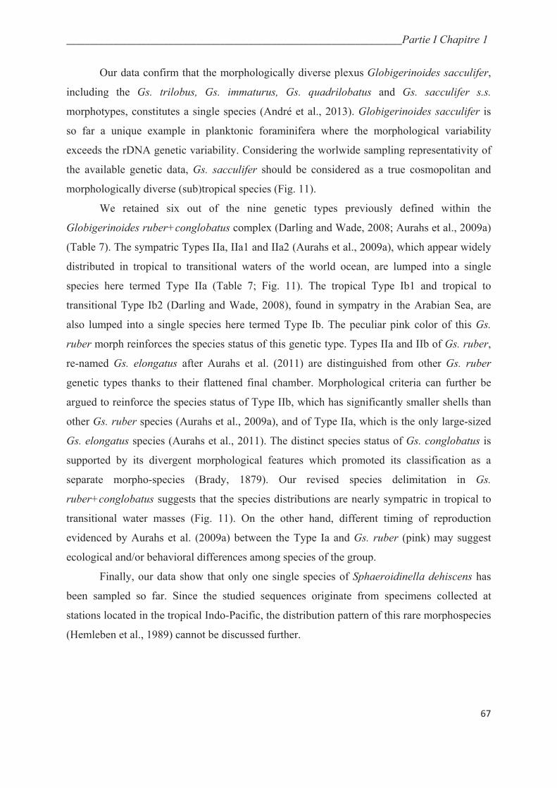
________________________________________________________________________Partie I Chapitre 1
67
Our data confirm that the morphologically diverse plexus Globigerinoides sacculifer,
including the Gs. trilobus, Gs. immaturus, Gs. quadrilobatus and Gs. sacculifer s.s.
morphotypes, constitutes a single species (André et al., 2013). Globigerinoides sacculifer is
so far a unique example in planktonic foraminifera where the morphological variability
exceeds the rDNA genetic variability. Considering the worlwide sampling representativity of
the available genetic data, Gs. sacculifer should be considered as a true cosmopolitan and
morphologically diverse (sub)tropical species (Fig. 11).
We retained six out of the nine genetic types previously defined within the
Globigerinoides ruber+conglobatus complex (Darling and Wade, 2008; Aurahs et al., 2009a)
(Table 7). The sympatric Types IIa, IIa1 and IIa2 (Aurahs et al., 2009a), which appear widely
distributed in tropical to transitional waters of the world ocean, are lumped into a single
species here termed Type IIa (Table 7; Fig. 11). The tropical Type Ib1 and tropical to
transitional Type Ib2 (Darling and Wade, 2008), found in sympatry in the Arabian Sea, are
also lumped into a single species here termed Type Ib. The peculiar pink color of this Gs.
ruber morph reinforces the species status of this genetic type. Types IIa and IIb of Gs. ruber,
re-named Gs. elongatus after Aurahs et al. (2011) are distinguished from other Gs. ruber
genetic types thanks to their flattened final chamber. Morphological criteria can further be
argued to reinforce the species status of Type IIb, which has significantly smaller shells than
other Gs. ruber species (Aurahs et al., 2009a), and of Type IIa, which is the only large-sized
Gs. elongatus species (Aurahs et al., 2011). The distinct species status of Gs. conglobatus is
supported by its divergent morphological features which promoted its classification as a
separate morpho-species (Brady, 1879). Our revised species delimitation in Gs.
ruber+conglobatus suggests that the species distributions are nearly sympatric in tropical to
transitional water masses (Fig. 11). On the other hand, different timing of reproduction
evidenced by Aurahs et al. (2009a) between the Type Ia and Gs. ruber (pink) may suggest
ecological and/or behavioral differences among species of the group.
Finally, our data show that only one single species of Sphaeroidinella dehiscens has
been sampled so far. Since the studied sequences originate from specimens collected at
stations located in the tropical Indo-Pacific, the distribution pattern of this rare morphospecies
(Hemleben et al., 1989) cannot be discussed further.

________________________________________________________________________Partie I Chapitre 1
68
5.5.2 Macroperforate non-spinose
Genetic sequencing studies have identified five genetic types within Truncorotalia
truncatulinoides (de Vargas et al., 2001; Ujiié et al., 2009), but applications of the ABGD and
GMYC methods suggest that this morpho-species harbors only 3 or 4 species, respectively
(Table 7). All methods agree on the species status of the right-coiled Type V (Ujiié et al.,
2009), which is apparently restricted to the NW Pacific where no other putative cryptic
species occurs (Fig. 11). ABGD is the only approach that significantly reduces intra-genetic
type and inter-genetic type patristic distances overlapping (Fig. 9B). It clusters Types I and II
on the one hand, and Types III and IV on the other hand (de Vargas et al., 2001), into two
distinct species with contrasted environmental affinities (Table 7). Type I-II is a warm water
species restricted to the (sub)tropical oceans, whereas Type III-IV appears to be restricted to
the productive subtropical and the colder subpolar frontal zones of the Southern Ocean (Fig.
11). Both species are pseudo-cryptic, since they can be differentiated on the basis of shell
morphology: Type I-II specimens exhibit large, highly conical left or right-coiled shells, and
Type III-IV specimens typically show smaller, axially-compressed and biconvex left-coiled
shells (Quillévéré et al., 2013).
Our data show that to date, no cryptic species have been sampled in the oceans for the
morpho-species Hirsutella hirsuta, Menardella menardii, Globorotalia tumida, Globorotalia
ungulata and Globoquadrina conglomerata (Table 7; Fig. 11). Considering the solid sampling
effort achieved for Ht. hirsuta in the Indian, Pacific and Atlantic Oceans (Fig. 11), we
speculate that Ht. hirsuta may be a single, cosmopolitan species of planktonic foraminifera.
The sequences available for M. menardii, Gr. tumida, Gr. ungulata and Gr. conglomerata
originate from too scarce and isolated locations of the world ocean (Fig. 11), then precluding
any further discussion about their cryptic diversity and biogeography.
Regarding Neogloboquadrina incompta, all methods agree on the species status of the
Types I and II of Darling et al. (2006). These two species have distinct distributions, the Type
I inhabiting the Southern Ocean and the North Atlantic, and the Type II inhabiting the North
Pacific (Darling et al., 2006; Fig. 11). Sequence AY453130, isolated as a possible third
species on the basis of GMYC analysis, is characterized by numerous substitutions that were
not found in any other N. incompta specimens from the NW Pacific (Kimoto and Tsuchiya,
unpublished), making the taxonomic status of this sequence unclear until further sampling.
Genetic sequencing studies have identified seven genetic types within
Neogloboquadrina pachyderma (Table 7, Darling and Wade, 2008) whose patristic distance

________________________________________________________________________Partie I Chapitre 1
69
values are compatible with a species status (Fig. 9A), although the distance gap is much
reduced. Application of the ABGD method leads to an alternative species delimitation
hypothesis which is also cross-validated by patristic distances (Table 7; Fig. 9B). The
distribution pattern of the genetic types defined in the literature tends to show that most of
them are allopatric and related to specific water masses (Fig. 11). The Type I was found in
polar waters of the North Atlantic (Darling et al., 2004). Types II, III and IV were found in
the Southern Ocean; Type IV appears to be a polar species, whereas Types II and III prefer
subpolar and transitional water masses (Darling et al., 2004). Types V and VI were only
collected in the South Atlantic, in the vicinity of the Benguela upwelling (Darling and Wade,
2008). Finally, specimens of Type VII seem to be restricted to transitional waters of the North
Pacific (Darling et al., 2007). Contrary to Darling et al. (2004), the ABGD method clusters all
sub-polar types from the South Hemisphere (Fig. 11), i.e., the Types II, III, V and VI, as a
single species.
Our study suggests that N. dutertrei constitutes a unique species that is cosmopolitan
in (sub)tropical waters of the world oceans (Table 7; Fig. 11). The GMYC method isolated the
sequence AY241708 as a putative second species (Fig. 10C). Because of its short length,
isolation of this sequence as a putative species may be an artifact. On the other hand, we
speculate that this sequence may represent another cryptic species restricted to the North
Pacific Ocean, a region that is known for harboring endemic cryptic species of planktonic
foraminifera (Darling and Wade, 2008).
Previous studies of the ITS genes have identified two genetic types of Globoconella
inflata (Morard et al., 2011). ABGD and patristic distances methods agree on the species
status of the Type I. However, due to the shortness of available sequences, these methods
cannot be used to test whether the Type II belongs to the same species as the Type I or is
indeed an independent species. Application of the GYMC method confirms the species status
of the Type I, which has been found to inhabit transitional to subtropical waters of both
hemispheres, and of the Type II, which is apparently restricted to the Antarctic subpolar
waters (Morard et al., 2011; Fig. 11). Species of Gc. inflata may be pseudo-cryptic, since
Morard et al. (2011) evidenced significant differences in shell morphology in modern
populations collected north and south of the Antarctic subpolar front.
Finally, genetic sequencing studies have identified three genetic types within
Pulleniatina obliquiloculata (Ujiié et al., 2012) but application of the ABGD and GMYC
methods suggest that those three types should be lumped into one or two species (Table 7).
________________________________________________________________________Partie I Chapitre 1
70
Patristic distances approach fails to cross-validate any of these delimitations (Fig. 9). Based
on GMYC analyses, the Type I (Ujiié et al., 2012) of P. obliquiloculata is an independent
species, when the Types IIa and IIb (Ujiié et al., 2012) constitute a single species. The Type I
of P. obliquiloculata occurs in tropical waters of the Indian and western Pacific Oceans (Fig.
11). In warmer waters of the tropical western Pacific, the Types I and II are found in sympatry
without any depth partitioning (Ujiié et al., 2012).
5.5.3. Microperforate clade
Up to now, no detailed genetic study has focused on the microperforate planktonic
foraminifera, probably because this clade includes rare morpho-species (Hemleben et al.,
1989), and because plankton net mesh and sieve sizes classically used for collecting living
foraminifera may have been too large for these typically small-sized taxa. Here, our models
for species delimitation are based solely on distance methods (patristic and ABGD), since
GYMC delimitations were not significantly better than the null hypothesis of a pure
coalescent model (Table 3).
For the sequences of Candeina nitida, estimation of patristic distance values (Fig. 9A)
suggests that only one cosmopolitan species has been sampled so far in the Caribbean Sea and
NW Pacific (Fig. 11).
Application of the ABGD method on the dataset of Globigerinita glutinata lumps the
sequences into four distinct clusters (Table 7) whose patristic distances are compatible with
the species status (Fig. 9B). Type I has been found in the subtropical north Atlantic, Type II in
the subtropical NW and SW Pacific, Type III in the subtropical north Atlantic and NW
Pacific, and Type IV has been found only in the Arabian Sea (Fig. 11). Considering the
tropical to polar waters geographic range of this morpho-species (Hemleben et al., 1989), we
speculate that yet unsampled cryptic species of Ga. glutinata may inhabit colder high latitude
surface waters.
Finally, application of the ABGD method on the dataset of Globigerinita uvula lumps
sequences into two distinct clusters (Table 7) whose patristic distances are compatible with
the species status (Fig. 9B). Such a species status of the Types I and II of Ga. uvula is
apparently reinforced on the basis of observational geographical data, which suggest that the
first species inhabits subtropical environments, when the second species may be restricted to
subpolar environments (Fig. 11).
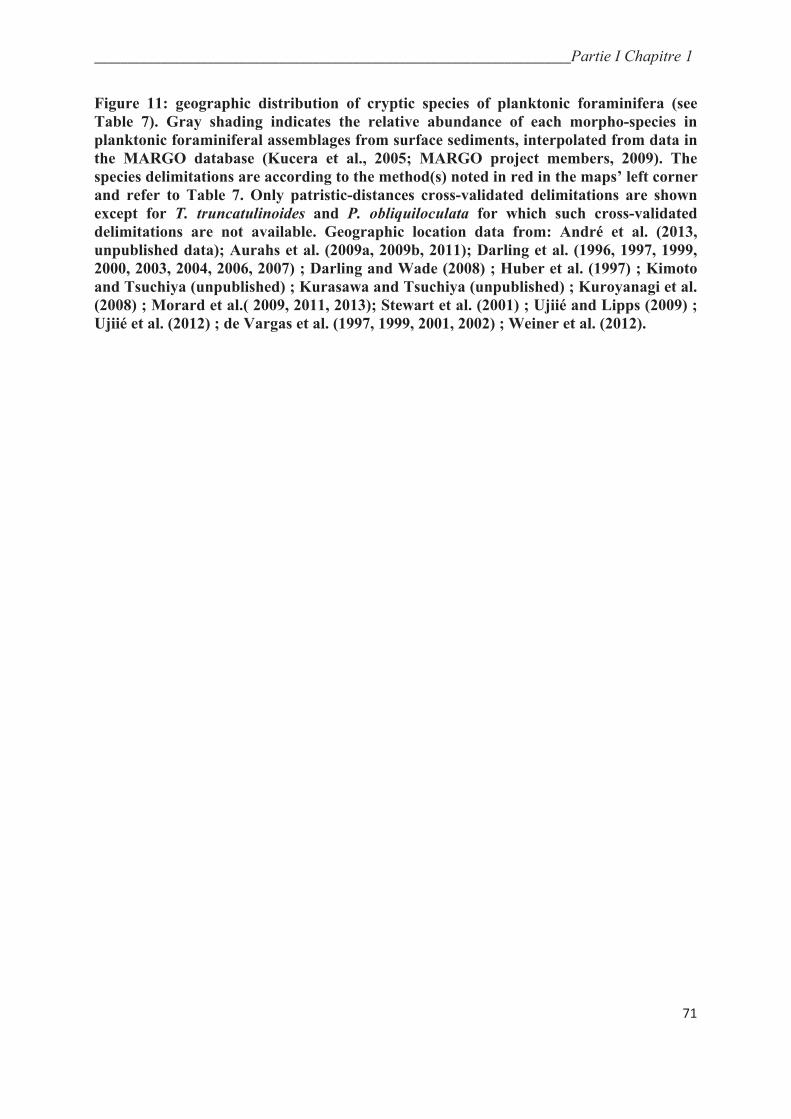
________________________________________________________________________Partie I Chapitre 1
71
Figure 11: geographic distribution of cryptic species of planktonic foraminifera (see
Table 7). Gray shading indicates the relative abundance of each morpho-species in
planktonic foraminiferal assemblages from surface sediments, interpolated from data in
the MARGO database (Kucera et al., 2005; MARGO project members, 2009). The
species delimitations are according to the method(s) noted in red in the maps’ left corner
and refer to Table 7. Only patristic-distances cross-validated delimitations are shown
except for T. truncatulinoides and P. obliquiloculata for which such cross-validated
delimitations are not available. Geographic location data from: André et al. (2013,
unpublished data); Aurahs et al. (2009a, 2009b, 2011); Darling et al. (1996, 1997, 1999,
2000, 2003, 2004, 2006, 2007) ; Darling and Wade (2008) ; Huber et al. (1997) ; Kimoto
and Tsuchiya (unpublished) ; Kurasawa and Tsuchiya (unpublished) ; Kuroyanagi et al.
(2008) ; Morard et al.( 2009, 2011, 2013); Stewart et al. (2001) ; Ujiié and Lipps (2009) ;
Ujiié et al. (2012) ; de Vargas et al. (1997, 1999, 2001, 2002) ; Weiner et al. (2012).
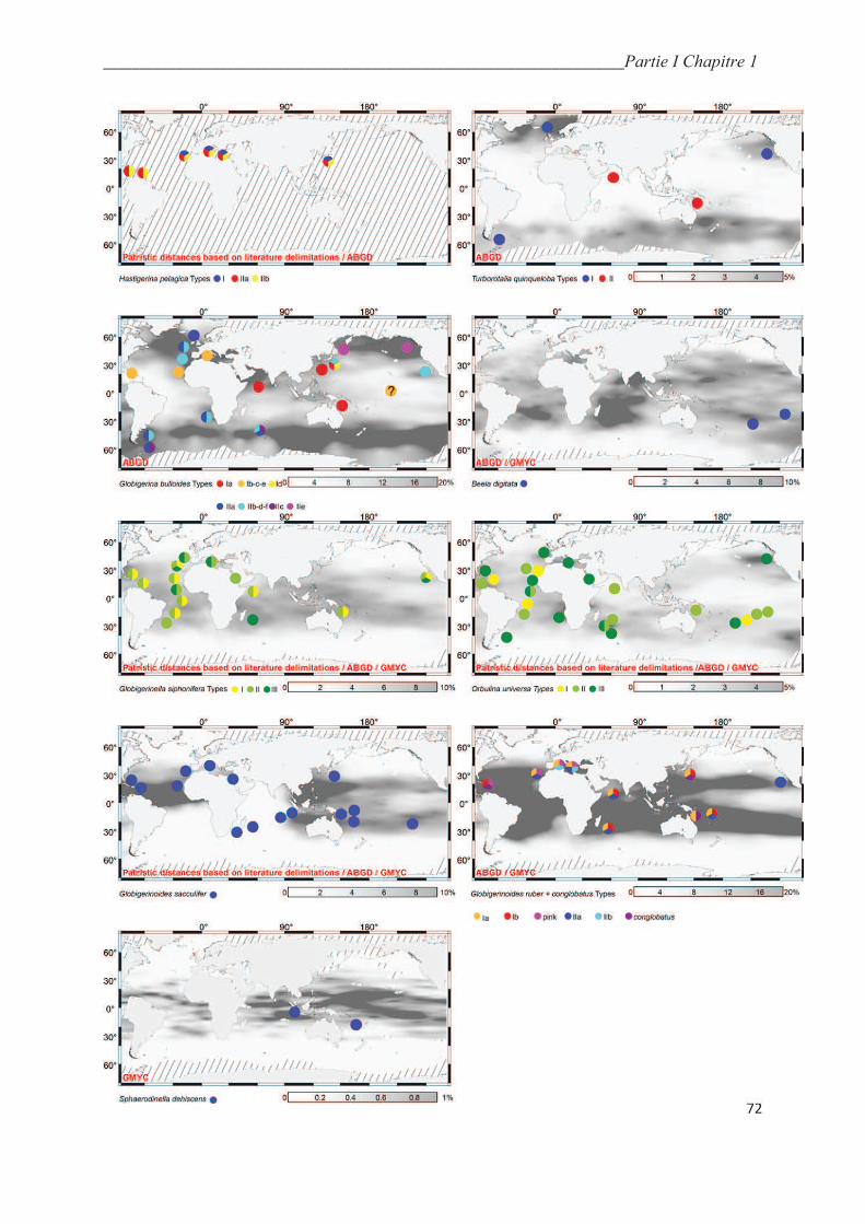
________________________________________________________________________Partie I Chapitre 1
72
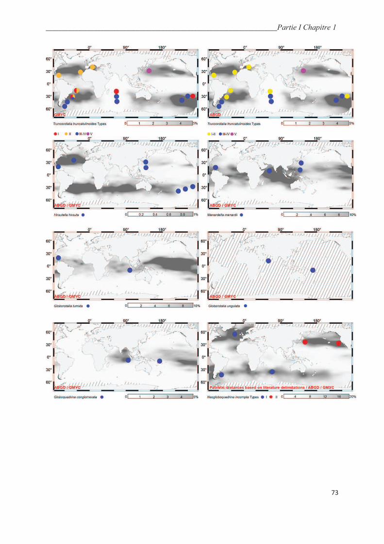
________________________________________________________________________Partie I Chapitre 1
73
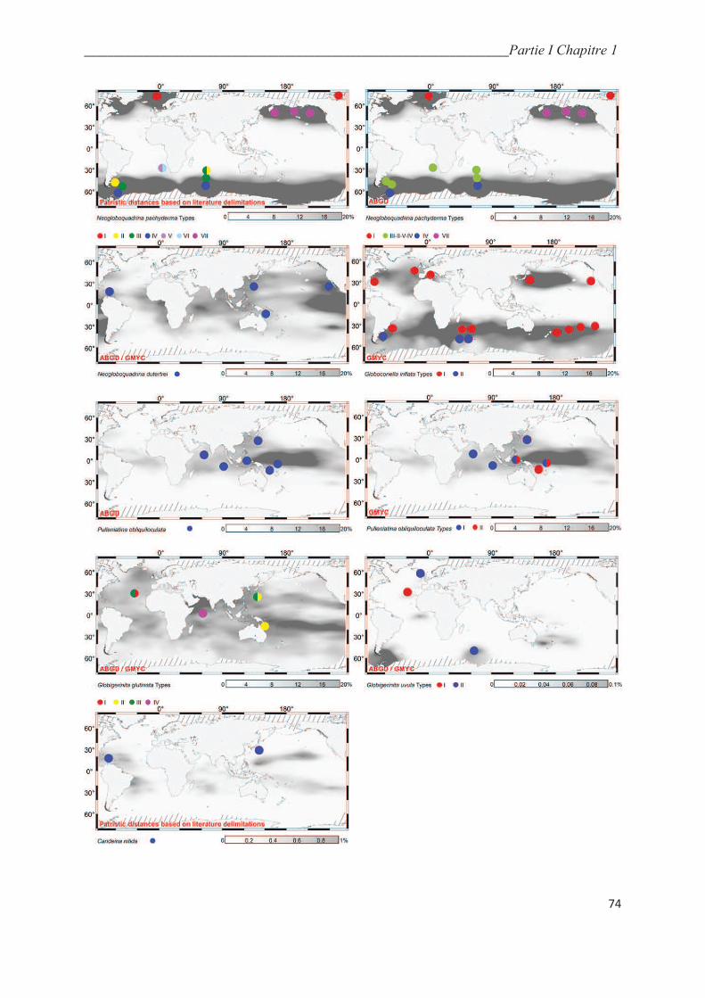
________________________________________________________________________Partie I Chapitre 1
74
________________________________________________________________________Partie I Chapitre 1
75
6. Conclusions
Two independent and quantitative methods, the ABGD and GMYC, coupled with
calculation of patristic distances within and among genetic types, were tested to quantify and
compare SSU rDNA divergences in planktonic foraminifera. Planktonic foraminiferal
putative species should be delimitated using these objective methods. The ABGD method
should be used in a first attempt because it is rapid and works at the morpho-species level. A
GMYC analysis may then be run in order to independently confirm the ABGD putative
species delimitations. Whenever delimitations are ambiguous or whenever several hypotheses
are possible, estimation of the patristic distances helps choosing the most plausible
delimitation. Nevertheless, our analyses show that the heterogeneity of sequence datasets is
detrimental for objective species delimitation. The ABGD method requires long enough and
strictly overlapping sequences. Consequently, the design of the ABGD dataset excluded part
of the original information, thus entirely excluding some potential cryptic species. Even if the
GMYC method requirements are less strict, our study shows that heterogeneity in length
and/or quality of the sequences can lead to non-significant results, causing unreliable species
delimitations. Furthermore, in the case of the GMYC method, more sequencing is required to
get significant species delimitations or to conclude on the taxonomic status of some of the
singletons defined by this method.
As a consequence, objective delimitation of foraminiferal cryptic species calls for a
standardization of the sequencing procedures. Sequence length should be standardized and
include at least the region used for species delimitation in this study. Several individuals
should be sequenced for each putative cryptic species in order to get a good estimation of the
intraspecific distances, which is crucial for ABGD and patristic distance methods, and in
order to enable GMYC to accurately identify the boundary between dichotomic (interspecific)
and coalescent (intra-specific) branching patterns. Several clones should be sequenced, at
least from a few individuals. Cloning gives the opportunity to estimate intragenomic distances
and to detect possible species oversplits whenever the automatic methods separate clones
from the same individuals into different putative species.
Our proposed taxonomic (re)assignment of planktonic foraminifera suggests that in
Globigerinella siphonifera (3 species), Globigerinoides sacculifer (1 species), Orbulina
universa (3 species), Hastigerina pelagica (3 species), Neogloboquadrina incompta (2
________________________________________________________________________Partie I Chapitre 1
76
species), Neogloboquadrina dutertrei (1 species) and Globoconella inflata (2 species), all the
genetic types defined in the literature correspond to (pseudo)cryptic species. In Beela digitata
(1 species), Sphaerodinella dehiscens (1 species), Hirsutella hirsuta (1 species),
Globoquadrina conglomerata (1 species), Menardella menardii (1 species), Globorotalia
ungulata (1 species), Globorotalia tumida (1 species), Globigerinita uvula (2 species),
Globigerinita glutinata (4 species) and Candeina nitida (1 species), 13 species are for the first
time delimited within the plankton-tow material available from the World Ocean. In
Turborotalia quinqueloba (2 species), Globigerina bulloides (7 species), and Globigerinoides
ruber+conglobatus (6 species), we show that only 15 out of the 26 previously described
genetic types constitute genuine species. Species delimitation within Truncorotalia
truncatulinoides (4 species), Neogloboquadrina pachyderma (4 species) and Pulleniatina
obliquiloculata (2 species) remains ambiguous, although our analyses suggest that some of
the characterized genetic types do not correspond to genuine species. All in all, our study
suggests that within the 55 genetic types described to date in the literature, only 29 constitute
cryptic or pseudo-cryptic species.
Such taxonomic (re)assignment complements and, in some cases modifies our
knowledge of the geographic distribution of planktonic foraminiferal species, which remains
complex with some species being cosmopolitan and others being narrower specialists.
Sampling sites are in most cases limited, studies of seasonal distribution variations are rare,
and the vertical distribution of species in the water column remains largely unknown,
preventing a finer understanding of the ecology (e.g., niche partitioning) and biogeographical
history of these species, especially when they are found sympatrically. From that point of
view, environmental sampling would be a great opportunity to better characterize the
distribution of planktonic foraminiferal cryptic species. Such datasets are bound to multiply as
high throughput sequencing methods are becoming more commonplace. Nevertheless, the
correct interpretation of environmental datasets first needs accurate species definitions, i.e., an
unambiguous reference database connecting sequences to identified true species, that we hope
promoting by this analysis.
________________________________________________________________________Partie I Chapitre 1
77
Acknowledgments
We thank T. Lefébure for his help with BEAST and G. Escarguel for comments on the
manuscript. We acknowledge the assistance of the Master and the crew of the cruises during
which the new material has been collected: AMT-8, Revelle, OISO, C-MarZ, Kt-02 and Kt-
06, Melville, Gyrafor A and B, FORCLIM. Special thanks are given to the Institut Polaire
Français Paul Emile Victor (IPEV). This work was supported by grants from the Institut
National des Sciences de l’Univers (INSU) INTERRVIE program (F.Q.).
Supplementary data 1
information on planktonic foraminifera sequences available on NCBI.
Supplementary data 2
A- sequence alignments; B- PhyML trees used for patristic distance calculation; C- BEAST
ultrametric trees; D- Patristic distance matrices.

____________________________________________________________Partie I Chapitre 1
78
References
Akaike, H., 1974. A new look at the statistical model identification. Institute of Electrical and
Electronics Engineers Transactions on Automatic Control, 19: 716-723.
Andersson, J.O., 2005. Lateral gene transfert in eucaryotes. Cellular and Molecular Life
Science, 62: 1182-1197.
André, A., Weiner, A., Quillévéré, F., Aurahs, R., Morard, R., Douady, C., de Garidel-
Thoron, T., Escarguel, G., de Vargas, C. and Kucera, M., 2013. The cryptic and the
apparent reversed: lack of genetic differentiation within the morphologically diverse
plexus of the planktonic foraminifer Globigerinoides sacculifer. Paleobiology, 39: 21-
39.
Aurahs, R., Göker, M., Grimm, G., Hemleben, V., Hemleben, C., Schiebel, R. and Kucera,
M., 2009. Using the multiple analysis approach to reconstruct phylogenetic
relationships among planktonic foraminifera from highly divergent and length-
polymorphic SSU rDNA sequences. Bioinformatics and Biology Insights, 3: 155-177.
Aurahs, R., Grimm, G., Hemleben, V., Hemleben, C. and Kucera, M., 2009. Geographical
distribution of cryptic genetic types in the planktonic foraminifer Globigerinoides
ruber. Molecular Ecology, 18: 1692-1706.
Aurahs, R., Treis, Y., Darling, K. and Kucera, M., 2011. A revised taxonomic and
phylogenetic concept for the planktonic foraminifer species Globigerinoides ruber
based on molecular and morphometric evidence. Marine Micropaleontology, 79: 1-14.
Bijma, J., Hemleben, C., Huber, B.T., Erlenkeuser, H. and Kroon, D., 1998. Experimental
determination of the ontogenetic stable isotope variability in two morphotypes of
Globigerinella siphonifera (d'Orbigny). Marine Micropaleontology, 35: 141-160.
Bolli, H. and Saunders, J., 1985. Oligocene to Holocene low latitude planktic foraminifera.
Plankton stratigraphy. Cambridge University Press, Cambridge.
Cavalier-Smith, T. and Chao, E.E.Y., 2003. Phylogeny and classification of phylum Cercozoa
(Protozoa). Protist, 154: 341-358.
Coleman, A.W., 2003. ITS2 is a double-edged tool for eukaryote evolutionary comparisons.
Trends in Genetics, 19: 370-375.
Coleman, A.W., 2009. Is there a molecular key to the level of “biological species” in
eukaryotes? A DNA guide. Molecular Phylogenetics and Evolution, 50: 197-203.
Darling, K.F., Kroon, D., Wade, C.M. and Leigh Brown, A.J., 1996. Molecular phylogeny of
the planktic foraminifera. Journal of Foraminiferal Research, 26: 324-330.
Darling, K.F., Wade, C.M., Kroon, D., Brown, A.J.L. and Bijma, J., 1999. The diversity and
distribution of modern planktic foraminiferal small subunit ribosomal RNA genotypes
and their potential as tracers of present and past circulation. Paleoceanography, 14: 3-
12.
Darling, K.F., Wade, C.M., Stewart, I.A., Kroon, D., Dingle R. and Brown, A.J., 2000.
Molecular evidence for genetic mixing of Arctic and Antarctic subpolar populations of
planktonic foraminifers. Nature, 405: 43-47.
____________________________________________________________Partie I Chapitre 1
79
Darling, K.F., Kucera, M., Wade, C.M., Langen, P.V. and Pak, D., 2003. Seasonal
distribution of genetic types of planktonic foraminifer morphospecies in the Santa
Barbara Channel and its paleoceanographic implications. Paleoceanography, 18: 1032-
1042.
Darling, K.F., Kucera, M., Pudsey, C.J. and Wade, C.M., 2004. Molecular evidence links
cryptic diversification in polar planktonic protists to Quaternary climate dynamics.
Proceedings of the National Academy of Science of the United States of America, 101:
7657-7662.
Darling, K.F., Kucera, M., Kroon, D. and Wade, C.M., 2006. A resolution for the coiling
direction paradox in Neogloboquadrina pachyderma. Paleoceanography, 21: 1-14.
Darling, K.F., Kucera, M. and Wade, C.M., 2007. Global molecular phylogeography reveals
persistent arctic circumpolar isolation in a marine planktonic protist. Proceedings of the
National Academy of Science of the United States of America, 104: 5002-5007.
Darling, K.F. and Wade, C.M., 2008. The genetic diversity of planktic foraminifera and the
global distribution of ribosomal RNA genotypes. Marine Micropaleontology, 67: 216-
238.
Dayrat, B., 2005. Towards integrative taxonomy. Biological Journal of the Linnean Society,
85: 407-415.
de Queiroz, K., 2007. Species concepts and species delimitation. Systematic Biology, 56:
879-886.
de Vargas, C., Zaninetti, L., Hilbrecht, H. and Pawlowski, J., 1997. Phylogeny and rates of
molecular evolution of planktonic foraminifera: SSU rDNA sequences compared to the
fossil record. Journal of Molecular Evolution, 45: 285-294.
de Vargas, C., Norris, R.D., Zaninetti, L., Gibb, S.W. and Pawlowski, J., 1999. Molecular
evidence of cryptic speciation in planktonic foraminifers and their relation to oceanic
provinces. Proceedings of the National Academy of Sciences of the United States of
America, 96: 2864-2868.
de Vargas, C., Renaud, S., Hilbrecht, H. and Pawlowski, J., 2001. Pleistocene adaptive
radiation in Globorotalia truncatulinoides: genetic, morphologic, and environmental
evidence. Paleobiology, 27: 104-125.
de Vargas, C., Bonzon, M., Rees, N.W., Pawlowski, J. and Zaninetti, L., 2002. A molecular
approach to biodiversity and biogeography in the planktonic foraminifer Globigerinella
siphonifera (d'Orbigny). Marine Micropaleontology, 45: 101-116.
Drummond, A.J., Suchard, M.A., Xie, D. and Rambaut, A., 2012. Bayesian phylogenetics
with BEAUti and the BEAST 1.7. Molecular Biology and Evolution, 8:1969-1973.
Ezard, T., Fujisawa, T. and Barraclough, T., 2009. Splits: SPecies' LImits by Threshold
Statistics. R package version 1.0-11/r29.
Fontaneto, D., Herniou, E.A., Boschetti, C., Caprioli, M., Melone, G., Ricci, C. and
Barraclough, T.G., 2007. Independently evolving species in asexual Bdelloid rotifers.
Public Library of Science Biology, 5: e87.

____________________________________________________________Partie I Chapitre 1
80
Görker, M., Grimm, G.W., Auch, A.F., Aurahs, R. and Kucera, M., 2010. A clustering
optimization strategy for molecular taxonomy applied to planktonic foraminifera SSU
rDNA. Evolutionary Bioinformatics, 6: 97-112.
Grimm, G.W., Stogerer, K., Ertan, K., Kitazato, H., Kucera, M., Hemleben, V. and
Hemleben, C., 2007. Diversity of rDNA in Chilostomella: molecular differentiation
patterns and putative hermit types. Marine Micropaleontology, 62: 75-90.
Guindon, S. and Gascuel, O., 2003. A simple, fast, and accurate algorithm to estimate large
phylogenies by maximum likelihood. Systematic Biology, 52:696-704.
Hammer, Ø., Harper, D.A.T. and Ryan, P.D., 2001. PAST: Paleontological statistics software
package for education and data analysis. Palaeontologia Electronica, 4: 9.
Hemleben, C., Spindler, M. and Anderson, O.R., 1989. Modern Planktonic Foraminifera.
Springer, New York.
Hoef-Emden, K., 2012. Pitfalls of establishing DNA barcoding systems in protists: the
Chrysophyceae as a test case. Public Library of Science One, 7: e45632.
Huber, B.T., Bijma, J. and Darling, K.F., 1997. Cryptic speciation in the living planktonic
foraminifer Globigerinella siphonifera (d'Orbigny). Paleobiology, 23: 33-62.
Katoh, K. and Toh, H., 2008. Recent developments in the MAFFT multiple sequence
alignment program. Briefings in Bioinformatics, 9: 276-285.
Kennett, J.P. and Srinivasan, M.S., 1983. Neogene Planktonic Foraminifera: a Phylogenetic
Atlas. Hutchinson Ross, Sroudsburg (Pennsylvania).
Kimoto, K. and Tsuchiya, M., unpublished. Coiling direction changes in different generations
of Neogloboquadrina pachyderma: importance on paleoceanographic reconstruction
from the evidence of laboratory cultivation and molecular phylogenetic analysis.
Kimura, M., 1980. A simple method for estimating evolutionary rates of base substitutions
through comparative studies of nucleotide sequences. Journal of Molecular Evolution,
16: 11-20.
Kucera, M., Rosell-Melé, A., Schneider, R., Waelbroeck, C. and Weinelt, M., 2005.
Multiproxy approach for the reconstruction of the glacial ocean surface (MARGO).
Quaternary Science Reviews, 24: 813-819.
Kucera, M., 2007. Planktonic foraminifera as tracers of past oceanic environments. Proxies in
Late Cenozoic Paleoceanography, Elsevier, Amsterdam.
Kurasawa, A., Tsuchiya, M., Toyofuku, T., Kitazato, H. and Nishi, H., unpublished. Genetic
variability of Globigerina bulloides in the Eastern North Pacific subtropical region and
the bipolarity of planktic foraminiferal genotypes.
Kuroyanagi, A., Tsuchiya, M., Kawahata, H. and Kitazato, H., 2008. The occurrence of two
genotypes of the planktonic foraminifer Globigerinoides ruber (white) and paleo-
environmental implications. Marine Micropaleontology, 68: 236-243.
Laetsch, D., Heitlinger, E., Taraschewski, H., Nadler, S. and Blaxter, M., 2012.The
phylogenetics of Anguillicolidae (Nematoda: Anguillicoloidea), swimbladder parasites
of eels. BioMed Central Evolutionary Biology, 12: 60.
Lee, J. J. and Anderson, O. R., 1991. Biology of Foraminifera. Academic Press, London.
____________________________________________________________Partie I Chapitre 1
81
Lefébure, T., Douady, C.J., Gouy, M. and Gibert, J., 2006. Relationship between
morphological taxonomy and molecular divergence within Crustacea: proposal of a
molecular threshold to help species delimitation. Molecular Phylogenetics and
Evolution, 40: 435-447.
Lemey, P., Rambaut, A., Welch, J.J. and Suchard, M.A., 2010. Phylogeography takes a
relaxed random walk in continuous space and time. Molecular Biology and Evolution,
27: 1877-1885.
Logares, R., Rengefors, K., Kremp, A., Shalchian-Tabrizi, K., Boltovskoy, A., Tengs, T.,
Shurtleff, A. and Klaveness, D., 2007. Phenotypically different microalgal
morphospecies with identical ribosomal DNA: a case of rapid adaptative evolution?
Microbial Ecology, 53: 549-561.
Maddison, W.P. and Knowles, L.L., 2006. Inferring phylogeny despite incomplete lineage
sorting. Systematic Biology, 55: 21-30.
Miralles, M. and Vence, A., 2013. New metrics for comparison of taxonomies reveal striking
discrepancies among species delimitation methods in Madascincus lizards. Public
Library of Science One, 8: e68242.
Morard, R., Quillévéré, F., Escarguel, G., Ujiie, Y., de Garidel-Thoron, T. Norris, R.D. and de
Vargas, C., 2009. Morphological recognition of cryptic species in the planktonic
foraminifer Orbulina universa. Marine Micropaleontology, 71: 148-165.
Morard, R., Quillévéré, F., Douady, C.J., de Vargas, C., de Garidel-Thoron, T. and Escarguel,
G., 2011.Worldwide Genotyping in the Planktonic Foraminifer Globoconella inflata:
Implications for Life History and Paleoceanography. Public Library of Science One, 6:
e26665.
Morard, R., Quillevere, F., Escarguel, G., de Garidel-Thoron, T., de Vargas, C. and Kucera,
M., 2013. Ecological modeling of the temperature dependence of cryptic species of
planktonic foraminifera in the Southern Hemisphere. Palaeogeography
Palaeoclimatology Palaeoecology. http://dx.doi.org/10.1016/j.palaeo.2013.05.011
Norris, R.D., 2000. Pelagic species diversity, biogeography and evolution. Paleobiology, 26:
236-258.
Pace, N.R., Olsen, G.J. and Woese, C.R., 1986. Ribosomal RNA phylogeny and the primary
lines of evolutionary descent. Cell, 45: 325-326.
Paradis, E., Claude, J. and Strimmer, K., 2004. APE: analyses of phylogenetics and evolution
in R language. Bioinformatics, 20: 289-290.
Parker, F.L., 1962. Planktonic foraminiferal species in Pacific sediments. Micropaleontology,
8: 219-254.
Pawlowski, J., Bolivar, I., Fahrni, J., de Vargas, C., Gouy, M. and Zaninetti, L., 1997.
Extreme differences in rates of molecular evolution of foraminifera revealed by
comparison of ribosomal DNA sequences and the fossil record. Molecular Biology and
Evolution, 14:498-505.
Pawlowski, J., 2000. Introduction to the molecular systematics of foraminifera.
Micropaleontology, 46: 1-12.
____________________________________________________________Partie I Chapitre 1
82
Pons, J., Barraclough, T.G., Gomez-Zurita, J., Cardoso, A., Duran, D.P., Hazell, S., Kamoun,
S., Sumlin, W.D. and Vogler, A.P., 2006. Sequence-based species delimitation for the
DNA taxonomy of undescribed insects. Systematic Biology, 55: 595-609.
Posada, D. and Crandall, K.A., 1998. Modeltest: testing the model of DNA substitution.
Bioinformatics, 14: 817-818.
Puillandre, N., Lambert, A., Brouillet, S. and Achaz, G., 2012. ABGD, Automatic Barcode
Gap Discovery for primary species delimitation. Molecular Ecology, 21: 1864-1877.
Puillandre, N., Modica, M.V., Zhang, Y., Sirovich, L., Boisselier, M.-C., Cruaud, C., Holford,
M. and Samadi, S., 2012. Large-scale species delimitation method for hyperdiverse
groups. Molecular Ecology, 21: 2671-2691.
Quillévéré, F., Morard, R., Escarguel, G., Douady, C.J., Ujiie, Y., de Garidel-Thoron, T. and
de Vargas, C., in press. Global scale same-specimen morpho-genetic analysis of
Truncorotalia truncatulinoides: A perspective on the morphological species concept in
planktonic foraminifera. Palaeogeography, Palaeoclimatology, Palaeoecology.
R Development Core Team, 2004. R: a language and environment for statistical computing.
Stewart, I.A., Darling, K.F., Kroon, D., Wade, C.M. and Troelstra, S.R., 2001. Genotypic
variability in subarctic Atlantic planktic foraminifera. Marine Micropaleontology, 43:
143-153.
Ujiie, Y. and Lipps, J.H., 2009. Cryptic diversity in planktic foraminifera in the northwest
Pacific Ocean. Journal of Foraminiferal Research, 39: 145-154.
Ujiié, Y., de Garidel-Thoron, T., Watanabe, S., Wiebe, P. and de Vargas, C., 2010. Coiling
dimorphism within a genetic type of the planktonic foraminifer Globorotalia
truncatulinoides. Marine Micropaleontology, 77: 145-153.
Weiner, A., Aurahs, R., Kurasawa, A., Kitazato, H. and Kucera, M., 2012. Vertical niche
partitioning between cryptic sibling species of a cosmopolitan marine planktonic protist.
Molecular Ecology, 21: 4063-4073.
________________________________________________________________________Partie I Chapitre 2
83
Chapitre 2 : apport des séquences complètes de la
SSU chez une morpho-espèce dont la délimitation
des types génétiques est problématique
Ce deuxième chapitre est une ébauche concernant la phylogénie des types génétiques
de Neogloboquadrina pachyderma et l’intérêt des séquences complètes de la SSU (petite
sous-unité ribosomale) chez une morpho-espèce dont la délimitation des types génétiques à
partir de séquences partielles reste problématique (chapitre 1). Diverses méthodes de
reconstruction phylogénétique ont été testées sur le jeu de données correspondant à la fin de la
SSU, ce qui a permis de mettre en évidence la grande sensibilité des reconstructions aux
conditions analytiques (méthode d’alignement et modèle de reconstruction phylogénétique)
chez N. pachyderma. Les premières séquences complètes de la SSU des Types II, III et IV de
N. pachyderma et du Type I de Neogloboquadrina incompta (hémisphère sud) ont été
obtenues ; elles s’ajoutent à la séquence du Type I de N. pachyderma et à celle du Type I de
N. incompta (hémisphère nord) disponibles dans la littérature. L’utilisation de séquences
complètes semble prometteuse pour résoudre la question des relations phylogénétiques au sein
de N. pachyderma, notamment parce que la région correspondant au début de la SSU est plus
variable que la fin. Déjà, les données acquises montrent qu’il est très probable que le premier
embranchement chez N. pachyderma corresponde au Type IV et non pas au Type I comme
précédemment publié, ce qui modifie alors le scénario évolutif au sein de cette morpho-
espèce. Cette étude nécessite néanmoins d’être encore approfondie, notamment par
l’obtention d’un plus grand nombre de séquences et le séquençage d’individus clonés afin
d’estimer la variabilité intra-génomique chez N. pachyderma.
Mots-clefs : Neogloboquadrina pachyderma, Neogloboquadrina incompta, séquences
complètes SSU, diversité cryptique, phylogénie
Fiches-méthodes : IV, V, VIII
Ont participé à ce chapitre : Aurore ANDRE (analyses, interprétation, rédaction), Frédéric
QUILLEVERE (rédaction)
________________________________________________________________________Partie I Chapitre 2
84
Des séquences complètes de la SSU peuvent-elles résoudre la
question des relations phylogénétiques entre les types génétiques
de Neogloboquadrina pachyderma (Ehrenberg) ?
Résumé
La définition des unités taxonomiques chez les foraminifères planctoniques ainsi que
leurs relations phylogénétiques sont établies à partir de séquences de la fin de la petite sous-
unité ribosomale (SSU). Les données actuellement disponibles pour la morpho-espèce
Neogloboquadrina pachyderma ne permettent cependant pas de conclure quant au statut
taxonomique de ses sept types génétiques et quant à leurs relations phylogénétiques. La
comparaison des arbres obtenus selon diverses méthodes montre que deux scénarios évolutifs
sont possibles, tous deux contredisant celui préalablement publié. Ces deux scénarios
considèrent que le premier embranchement chez N. pachyderma correspond à l’adaptation du
Type IV aux conditions polaires extrêmes de l’océan austral. La rupture du flux génétique
entre les deux hémisphères est plus tardive et pourrait être liée à la mise en place des cycles
glaciaire-interglaciaires de 100ka, il y a environ 1 Ma. Les relations au sein du clade formé
par les N. pachyderma subantarctiques (Types II, III, V et VI) ne sont pas résolues, ce qui
pourrait suggérer que ces types génétiques ne correspondent pas tous à des espèces cryptiques
distinctes. L’étude des séquences complètes de la SSU chez les Types I, II, III et IV de N.
pachyderma et chez N. incompta montre que la variabilité génétique est répartie de façon non
homogène le long de la SSU et en particulier que le début de la SSU est plus variable que la
fin. Les reconstructions obtenues à partir de ces séquences favorisent l’hypothèse du Type IV
comme branche basale. La comparaison des séquences complètes semble montrer que Types
II et III peuvent être deux espèces distinctes et qu’il existe des différences génétiques entre les
Types I de N. incompta des hémisphères nord et sud. Le séquençage complet de la SSU, bien
que techniquement difficile, est donc prometteur à la fois pour la résolution des relations
phylogénétiques et pour la délimitation des unités taxonomiques chez N. pachyderma.
Mots-clef : phylogénie, SSU complète, diversité cryptique, Neogloboquadrina pachyderma
________________________________________________________________________Partie I Chapitre 2
85
Abstract
Planktonic foraminiferal species delimitation and phylogeny are based on partial 3’
end sequences of the ribosomal small sub-unit (SSU). These data are still insufficient to reach
a consensus on the delimitation of the genetic types of Neogloboquadrina pachyderma. The
phylogeny of its seven possible genetic types also remains unsolved. Two different tree
topologies are possible according to comparisons of phylogenetic trees obtained through
various reconstruction methods. Both these topologies are in conflict with the published
Neogloboquadrinid tree. The ensuing new evolutionary history hypotheses suggest that the
austral Type IV of N. pachyderma diverged first when it acquired its extreme polar affinities.
The transequatorial gene flow stopped later, possibly as a consequence of the 100 kyr glacial
cycles onset that occurred about 1 myrs ago. Phylogenetic relationships between the genetic
types among the sub-Antarctic clade (Types II, III, V, VI) are unclear, suggesting that some of
these types may correspond to intra-specific variants. Complete SSU sequences of the Types
I, II, III and IV of N. pachyderma and the Type I of N. incompta show that variable regions
are concentrated on the 5’ end of the SSU whereas the 3’ end corresponds to more conserved
regions. Reconstructions based on complete sequences support the Type IV as the earliest
diverging genetic type. Comparisons of complete sequences of the SSU suggest that the
Types II and III may indeed correspond to distinct species. Likewise, genetic divergence
between southern and northern hemisphere Types I of N. incompta is for the first time
evidenced. Although complete sequencing of planktonic foraminiferal SSU is technically
difficult and time consuming, it is a challenging opportunity to resolve delimitations and
phylogeny within N. pachyderma.
Keywords: phylogeny, complete SSU, cryptic diversity, Neogloboquadrina pachyderma
________________________________________________________________________Partie I Chapitre 2
86
1. Introduction
De nombreuses études ont montré que les morpho-espèces de foraminifères planctoniques
regroupent jusqu’à sept unités taxonomiques (André et al., en préparation A ; cette thèse,
Partie I Chapitre 1), souvent appelées espèces cryptiques (par exemple, Weiner et al., 2012)
ou types génétiques (par exemple, Ujiié et al., 2010), qui peuvent être prises en compte afin
d’améliorer la précision des fonctions de transfert utilisées pour les reconstructions
paléocéanographiques au Quaternaire (Morard et al., 2013). La définition de ces unités
taxonomiques ainsi que leurs relations phylogénétiques sont établies à partir de séquences de
l’extrémité 3’ de la petite sous-unité ribosomale (SSU) (par exemple : Darling et Wade,
2008 ; Aurahs et al., 2009 ; André et al., en préparation A). Or, pour une utilisation optimale
des foraminifères planctoniques en tant que proxy paléoclimatique, une délimitation
rigoureuse de ces unités taxonomiques est un pré-requis (Kucera et Darling, 2002).
Neogloboquadrina pachyderma est une espèce-clef pour les reconstructions
paléoclimatiques en hautes latitudes où elle représente jusqu’à 100 % des assemblages de
foraminifères planctoniques (base de données MARGO, 2009). Neogloboquadrina
pachyderma est aussi un marqueur biostratigraphique aux hautes latitudes; ainsi son
apparition dans les sédiments de l’Atlantique nord marque le passage entre Pliocène et
Pléistocène (Speigler et Janssen, 1989). L’histoire évolutive de N. pachyderma est fortement
liée à celle des glaciations qui sont une caractéristique majeure du climat de ces derniers
millions d’années (Bartoli et al., 2005 ; Becquey et al., 2003). Démêler la phylogéographie
des différents types génétiques de N. pachyderma est donc une opportunité de mieux
comprendre l’histoire climatique du Quaternaire et son impact sur l’évolution des
foraminifères planctoniques.
La délimitation des unités taxonomiques au sein de la morpho-espèce Neogloboquadrina
pachyderma pose problème. Sept types génétiques ont été initialement définis par Darling et
al. (2004 ; 2007) (Fig. 12) mais André et al. (en préparation A) ont montré qu’un découpage
en quatre unité taxonomiques seulement est également probable. Dans cette hypothèse, les N.
pachyderma subantarctiques, c’est-à-dire les Types II, III, V, VI sensu Darling et al. (2004),
forment une seule et même espèce. Les données biogéographiques et environnementales ne
permettent pas de trancher entre ces deux délimitations. André et al. (en préparation B) ont
établi que le Type II a des affinités écologiques plus restreintes que le Type III mais ces deux
types génétiques présentent néanmoins des distributions biogéographiques qui se recouvrent.

________________________________________________________________________Partie I Chapitre 2
87
De plus, aucune différence de profondeur de milieu de vie et /ou de saison de reproduction n’a
encore pu être clairement mise en évidence. Darling et al. (2004) ont montré que les Types V
et VI sont isolés dans l’upwelling du Benguela mais les données disponibles sur ces types
génétiques sont encore très insuffisantes. Des individus d’affinités subantarctiques ont en effet
pu envahir l’upwelling du Benguela lors du déplacement vers le nord de la convergence
subtropicale au cours des glaciations quaternaires (Ufkes et al., 2000). La question qui se pose
est donc de comprendre si le flux génétique a ensuite pu être réduit voire interrompu durant
les périodes interglaciaires.
Figure 12 : distribution schématique des types génétiques de Neogloboquadrina
pachyderma sensu Darling et al. (2007) (Darling et al., 2004 ; 2007 ; André et al., en
préparation B). Localisation des échantillons utilisés pour obtenir les séquences
complètes de la SSU (Inc. : Neogloboquadrina incompta (Type I), I : N. pachyderma Type
I, II : N. pachyderma Type II, III : N. pachyderma Type III, IV : N. pachyderma Type
IV).
Schweizer et al. (2008) ont montré que les phylogénies des foraminifères benthiques
obtenues à partir de séquences complètes de la SSU sont plus robustes que celles basées sur
les séquences de la fin de cette région ; chez les foraminifères planctoniques, Seears (2011) a
montré que les séquences complètes de la SSU sont effectivement plus informatives même si
elles restent insuffisantes pour la résolution des nœuds basaux entre les grands clades. Dans
________________________________________________________________________Partie I Chapitre 2
88
cette étude, au contraire, nous allons tenter de réaliser une phylogénie à l’échelle de la
morpho-espèce utilisant des séquences complètes de la SSU. De telles reconstructions
impliquent des séquences peu divergentes, ce qui réduit donc la taille des régions non
alignables, peu informatives, qui se sont révélées constituer un obstacle majeur pour les
reconstructions phylogénétiques à plus grande échelle (Seears, 2011). Utiliser des séquences
complètes de la SSU semble particulièrement intéressant dans le cas des morpho-espèces
comme N. pachyderma, pour lesquelles la définition des unités taxonomiques pose problème
(André et al., en préparation A). Cependant, les séquences complètes restent rares chez les
foraminifères planctoniques. Seulement 16 séquences complètes ou sub-complètes sont
disponibles sur NCBI (Neogloboquadrina dutertrei, Hirsutella hirsuta et Globoconella
inflata, Schweizer et al., 2008) ou dans les travaux de thèse de Seears (2011) (Globigerina
bulloides, Globigerinoides sacculifer, Globigerinita glutinata, Neogloboquadrina dutertrei,
Pulleniatina obliquiloculata, Globoconella inflata, Neogloboquadrina incompta Type I,
Globigerinita uvula, Neogloboquadrina pachyderma Type I, Globorotalia ungulata,
Menardella menardii et Streptochilus globigerus).
Cette étude se propose de revenir sur les reconstructions phylogénétiques de N.
pachyderma basées sur la fin de la SSU afin de mettre clairement en évidence les
embranchements résolus mais aussi ceux qui ne le sont pas. La première tentative de
délimitation objective des types génétiques de N. pachyderma (André et al., en préparation A)
a suggéré que la topologie de l’arbre, et donc le scénario évolutif proposé par Darling et al.
(2007) pourraient être remis en cause. Cette étude présente donc de nouvelles hypothèses
phylogéographiques retraçant l’histoire des types génétiques de N. pachyderma. Au vu de
l’insuffisance de ces données à la fois pour résoudre les questions de phylogénie et de
délimitation des unités taxonomiques, des séquences complètes de la SSU des Types II, III et
IV de N. pachyderma et du Type I de N. incompta ont été obtenues pour la première fois. Les
séquences sub-complètes du Type I de N. pachyderma et du Type I de N. incompta obtenues
pas Seears (2001) viennent compléter ce jeu de données. L’identification des régions
conservées et variables à plusieurs échelles permet de mieux estimer la divergence entre les
différents types génétiques. Une première tentative de phylogénie permet de tester la
robustesse des différents scénarios évolutifs proposés.

________________________________________________________________________Partie I Chapitre 2
89
2. Matériel et Méthodes
2.1. Reconstructions phylogénétiques à partir des séquences de la fin de la SSU
Les séquences publiées correspondant à la fin de la SSU de Neogloboquadrina
pachyderma (n=17), Neogloboquadrina incompta (n=13), Neogloboquadrina dutertrei
(n=10), une séquence de Globoconella inflata (NCBI Z83971, de Vargas et al., 1997) et une
de Pulleniatina obliquiloculata (NCBI AY241709, Darling et al., 2003) ont été compilées à
partir de NCBI (14 Juin 2013). Les séquences de N. pachyderma de génotype non identifié
provenant du Pacifique Nord ont été attribuées au Type VII comme le suggèrent André et al.
(en préparation A) et Darling et al. (2007).
Plusieurs méthodes d’alignement de séquences et de reconstruction phylogénétique
associés à différents groupes externes ont été employées afin d’estimer la sensibilité des
reconstructions phylogénétiques aux conditions analytiques chez N. pachyderma. Pour
s’affranchir de la subjectivité et de la non-reproductibilité d’un alignement manuel, les
séquences ont été alignées automatiquement grâce aux programmes MUSCLE v.3.7 (Edgar,
2004) et MAFFT v.7. (Katoh et Toh, 2008). Les régions dont l’alignement est ambigu ont été
retirées grâce à GBlocks 0.91b (Castresana, 2000). Cependant, comme la taille des fragments
obtenus est alors très réduite (279 à 404 pb), des analyses ont aussi été réalisées sur les
alignements bruts. Trois groupes externes ont été testés : N. dutertrei seul, N. dutertrei et N.
incompta ; N. dutertrei, P. obliquiloculata et G. inflata. Ce dernier cas correspond à celui
utilisé dans la seule phylogénie complète des types génétiques de N. pachyderma publiée
(Darling et al., 2007). Les arbres phylogénétiques ont été générés grâce aux différentes
méthodes implémentées dans SEAVIEW v.4.1. (Gouy et al., 2009) : maximum de
vraisemblance (PhyML, Guidon et Gascuel, 2003), Neighbour-Joining (Saitou et Nei, 1987 ;
Studier et Keppler, 1988) et une variante du Neighbour-Joining, BIONJ (Gascuel, 1997).
Dans le cas des arbres générés par PHYML, les modèles de substitution nucléotidique les plus
appropriés selon l’Akaike Information Criterion (AIC, Akaike, 1974) ont été choisis grâce au
logiciel MODELTEST 0.1.1. (Posada et Crandall, 1998). La robustesse des nœuds a été
estimée à l’aide de 1000 « bootstraps ». Ces arbres ont été enracinés manuellement grâce aux
groupes externes. Les différentes topologies obtenues ont été reportées, la longueur des
branches n’est pas prise en compte dans cette étude.
________________________________________________________________________Partie I Chapitre 2
90
2.2. Obtention de séquences complètes de la SSU
Trois N. pachyderma correspondant aux Types II, III et IV (Darling et al. 2004) et une N.
incompta de Type I (Darling et al., 2006) ont été sélectionnées parmi les individus récoltés
dans le sud de l’Océan Iindien lors de la campagne OISO-21, à la fin de l’été austral de
l’année 2012 (Fig. 12 ; André et al., en préparation B). Les Types II et III de N. pachyderma
ainsi que le Type I de N. incompta proviennent de la station 7 (47,5°S, 57.5°E) et le spécimen
de Type IV de N. pachyderma a été récolté sur la station 11 (56°S, 63°E). Leur ADN a été
préalablement extrait et la fin de la SSU séquencée afin d’identifier leur type génétique selon
la méthode décrite par André et al. (en préparation B). Ces N. pachyderma et N. incompta ont
été choisis pour leur rendement d’amplification par PCR particulièrement bon au vu de
l’épaisseur des bandes visualisées par électrophorèse après amplification de l’ADN.
Afin d’établir les séquences complètes de la SSU, un ensemble de fragments courts et
longs ont été amplifiés (Tables 8 et 9 Fig. 13) grâce à de nouvelles amorces venant compléter
celles disponibles dans la littérature (Table 8). L’amplification par PCR suit la procédure
décrite par André et al. (en préparation B) avec, pour les fragments longs (>1000 pb) un
temps de polymérisation augmenté (3 min au lieu de 30s). Les tentatives de clonage ayant
échoué, les séquences ont été obtenues par séquençage direct selon la méthode de Sanger
(Smith et al., 1986) par Biofidal (Vaulx-en-Velin, France) à l’aide d’un séquenceur ABI prism
3730XL (Applied Biosystems). Seules ont été conservées les régions dont le
chromatogramme était non ambigu, ce qui a nécessité l’amplification de multiples fragments
partiellement redondants (Fig. 13). Les fragments courts ont été séquencés dans les deux sens
avec les amorces utilisées pour l’amplification alors que les fragments longs ont été séquencés
en plusieurs parties à l’aide d’amorces internes, car la réaction de séquençage est peu efficace
au-delà de 500 à 1000 pb selon les individus. Les fragments ont ensuite été alignés
manuellement grâce au logiciel SEAVIEW (Gouy et al., 2009) puis concaténés afin d’obtenir
la séquence complète. La redondance des fragments a facilité cette étape.
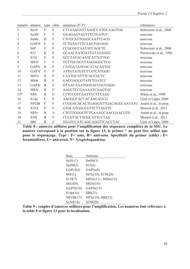
________________________________________________________________________Partie I Chapitre 2
91
numéro amorce type cible séquence (5'-3') réferences
1 Sa10 F F CTTAAAGATTAAGCCATGCAAGTGG Schweizer et al., 2008
2 Sa30f F F GAAGAGTAGTTTCTGATCC nouveau
3 Sa60r R F CTGTCATTGGGCAATTTACG nouveau
4 GAP1f F F TCTGAATTTCAAGTGGAGG nouveau
5 S6F F F CCGCGGTAATACCAGCTC Schweizer et al., 2008
6 S13 R F GCAACAATGATTGTATAGGC Pawlowski et al., 1996
7 S13f F F GCCTATACAATCATTGTTGC nouveau
8 MS1f F F TGTTGCGGTTAAGAGGCTCG nouveau
9 GAP5r R F CATGATAAGACATACAATGC nouveau
10 GAP3f F F ATTGTATGTCTTATCATGGG nouveau
11 MD1r R F CAATGCATTTCACCGCTC nouveau
12 MS4r R F GACGAGGGTATCTGATCC nouveau
13 GAP4r R F GTAACAAATGGGACGACGAGG nouveau
14 MS3r R F AAGCTCCGAAAATCAAGTGC nouveau
15* NS4 R U CTTCCGTCAATTCCTTTAAG White et al., 1990
16 S14p F F AAGGGCACCACAAGAGCG Ujiié et Lipps, 2009
17 NP1fB F F CCGGACACACTGAGGATTGACAGGCAATATC André et al., in prep.
18 S15rf F F GTGCATGGCCGTTCTTAGTTC Morard et al., 2011
19 NP5r R N CTGTTGGGCTCTGAAAGCAACGAACGTG André et al., in prep.
20 S19f R F CCCGTACTAGGCATTCCTAG Morard et al., 2011
21 SBf R F TGATCCATCAGCAGGTTCACCTAC Ujiié et Lipps, 2009
Table 8 : amorces utilisées pour l’amplification des séquences complètes de la SSU. Le
numéro correspond à la position sur la figure 13, le primer * ne peut être utilisé que
pour le séquençage. Type : F= sens, R= anti-sens. Spécificité du primer (cible) : F=
foraminifères, U= universel, N= Neogloboquadrina.
Sens Antisens
Sa10 (1) Sa60r(3)
Sa30f(2) S13(6)
GAP1f(4) GAP5r(9)
S6F(5) NP5r(19), S19f(20)
S13f(7) MD1r(11) , MS4r(12)
MS1f(8) MS3r(14)
GAP3f(10) GAP4r(13)
S14p(16) SBf(21)
NP1fB(17) NP5r(19), SBf(21)
S15rf(18) S19f(20)
Table 9 : couples d’amorces utilisées pour l’amplification. Les numéros font référence à
la table 8 et figure 13 pour la localisation.
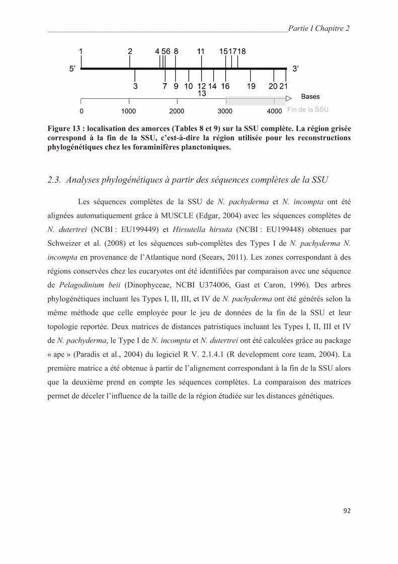
________________________________________________________________________Partie I Chapitre 2
92
Figure 13 : localisation des amorces (Tables 8 et 9) sur la SSU complète. La région grisée
correspond à la fin de la SSU, c’est-à-dire la région utilisée pour les reconstructions
phylogénétiques chez les foraminifères planctoniques.
2.3. Analyses phylogénétiques à partir des séquences complètes de la SSU
Les séquences complètes de la SSU de N. pachyderma et N. incompta ont été
alignées automatiquement grâce à MUSCLE (Edgar, 2004) avec les séquences complètes de
N. dutertrei (NCBI : EU199449) et Hirsutella hirsuta (NCBI : EU199448) obtenues par
Schweizer et al. (2008) et les séquences sub-complètes des Types I de N. pachyderma N.
incompta en provenance de l’Atlantique nord (Seears, 2011). Les zones correspondant à des
régions conservées chez les eucaryotes ont été identifiées par comparaison avec une séquence
de Pelagodinium beii (Dinophyceae, NCBI U374006, Gast et Caron, 1996). Des arbres
phylogénétiques incluant les Types I, II, III, et IV de N. pachyderma ont été générés selon la
même méthode que celle employée pour le jeu de données de la fin de la SSU et leur
topologie reportée. Deux matrices de distances patristiques incluant les Types I, II, III et IV
de N. pachyderma, le Type I de N. incompta et N. dutertrei ont été calculées grâce au package
« ape » (Paradis et al., 2004) du logiciel R V. 2.1.4.1 (R development core team, 2004). La
première matrice a été obtenue à partir de l’alignement correspondant à la fin de la SSU alors
que la deuxième prend en compte les séquences complètes. La comparaison des matrices
permet de déceler l’influence de la taille de la région étudiée sur les distances génétiques.
________________________________________________________________________Partie I Chapitre 2
93
3. Résultats
3.1. Analyses phylogénétiques obtenues à partir des séquences de la fin de la
SSU
Trente-six arbres phylogénétiques ont été générés. Cependant, onze d’entre eux
présentent des nœuds irrésolus et trois d’entre eux ne respectent pas la monophylie des
morpho-espèces. Au final, vingt-deux arbres peuvent donc être considérés comme plausibles
(Table 10). Ces 22 arbres présentent 10 topologies différentes mais aucune d’entre elles ne
correspond à celle proposée par Darling et al. (2007) (Fig. 14). Les reconstructions
phylogénétiques chez Neogloboquadrina pachyderma sont très sensibles aux méthodes
employées et aucune topologie ne fait consensus. Ainsi, modifier la méthode d’alignement
des séquences modifie la topologie de l’arbre dans 50 % des cas ; de même, retirer les régions
difficilement alignables entraine l’obtention d’une nouvelle topologie ; enfin, pour un même
alignement, il n’y a concordance entre les trois méthodes de reconstruction que dans un cas
sur cinq (Table 10). L’utilisation de Gblocks (Castresana, 2000) pour s’affranchir du bruit
découlant de la présence de régions difficilement alignables s’est révélée peu fructueuse : 13
des 14 arbres non résolus ont été obtenus à partir de tels alignements (Table 10). Ce
phénomène n’est pas inattendu car les alignements obtenus sont très courts (279 à 404 pb), ce
qui réduit drastiquement le signal phylogénétique. Néanmoins, tous les arbres générés
proposent le Type IV comme branche basale et considèrent que les Types subantarctiques, en
incluant les types récoltés dans l’upwelling du Benguela (Types II, III, V et VI sensu Darling
et al., 2007) forment un clade. Ces embranchements sont bien soutenus : en moyenne 84 %
pour l’embranchement du Type IV et 89% pour le clade subantarctique.
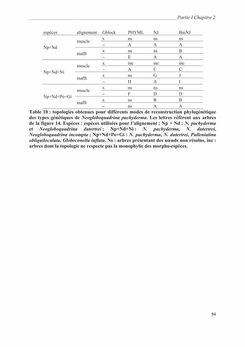
________________________________________________________________________Partie I Chapitre 2
94
espèces alignement Gblock PHYML NJ BioNJ
Np+Nd
muscle x ns ns ns
– A A A
mafft x ns ns B
– E A A
Np+Nd+Ni
muscle x inc inc inc
– A C C
mafft x ns G J
– H A I
Np+Nd+Po+Gi
muscle x ns ns ns
– F D D
mafft x ns B B
– ns A A
Table 10 : topologies obtenues pour différents modes de reconstruction phylogénétique
des types génétiques de Neogloboquadrina pachyderma. Les lettres réfèrent aux arbres
de la figure 14. Espèces : espèces utilisées pour l’alignement ; Np + Nd : N. pachyderma
et Neogloboquadrina dutertrei ; Np+Nd+Ni : N. pachyderma, N. dutertrei,
Neogloboquadrina incompta ; Np+Nd+Po+Gi : N. pachyderma, N. dutertrei, Pulleniatina
obliquiloculata, Globoconella inflata. Ns : arbres présentant des nœuds non résolus, inc :
arbres dont la topologie ne respecte pas la monophylie des morpho-espèces.
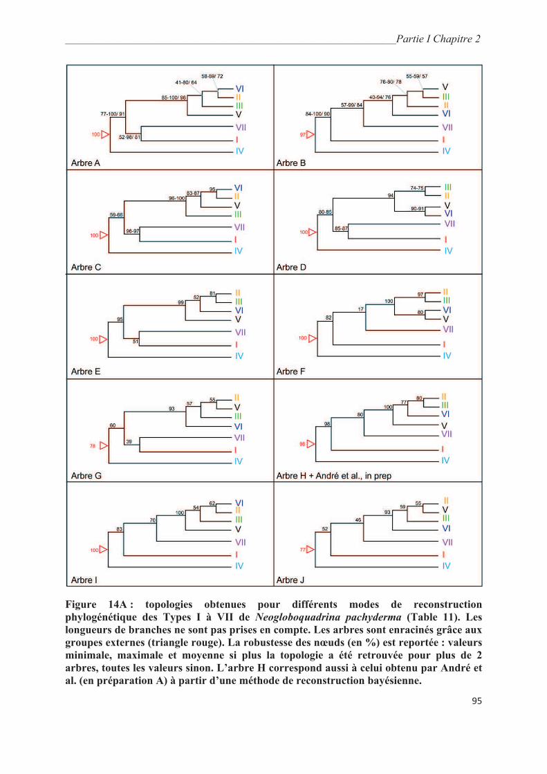
________________________________________________________________________Partie I Chapitre 2
95
Figure 14A : topologies obtenues pour différents modes de reconstruction
phylogénétique des Types I à VII de Neogloboquadrina pachyderma (Table 11). Les
longueurs de branches ne sont pas prises en compte. Les arbres sont enracinés grâce aux
groupes externes (triangle rouge). La robustesse des nœuds (en %) est reportée : valeurs
minimale, maximale et moyenne si plus la topologie a été retrouvée pour plus de 2
arbres, toutes les valeurs sinon. L’arbre H correspond aussi à celui obtenu par André et
al. (en préparation A) à partir d’une méthode de reconstruction bayésienne.
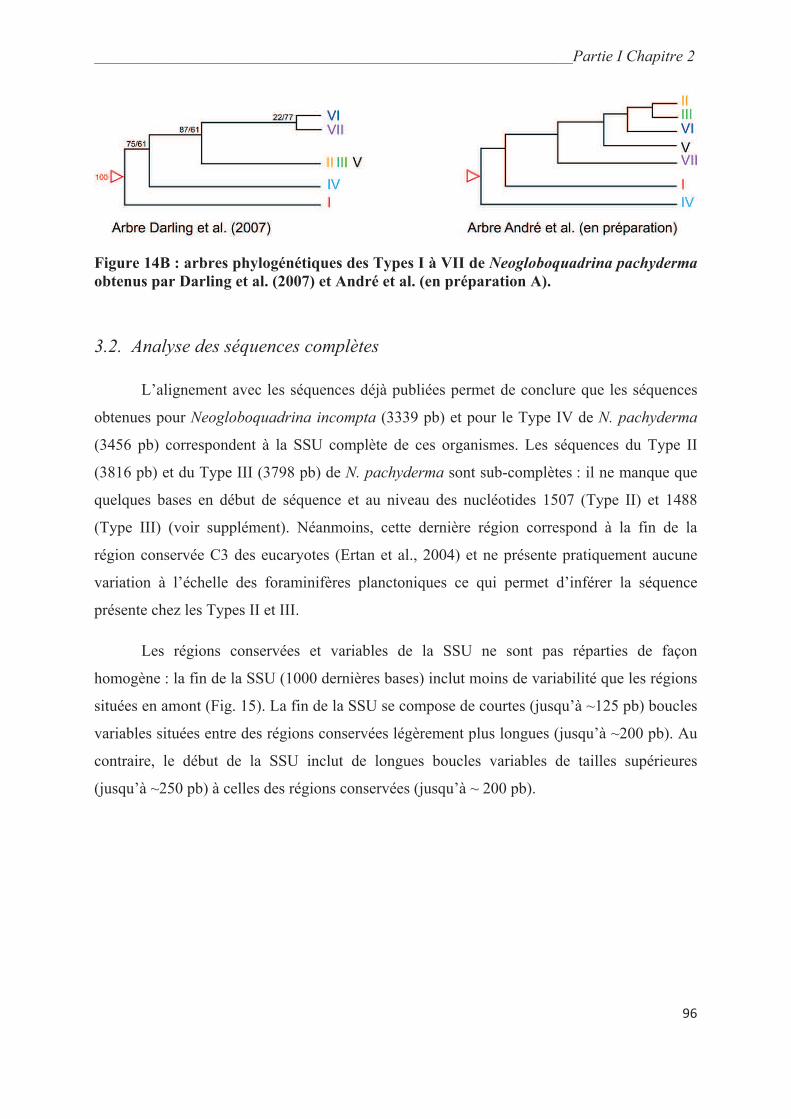
________________________________________________________________________Partie I Chapitre 2
96
Figure 14B : arbres phylogénétiques des Types I à VII de Neogloboquadrina pachyderma
obtenus par Darling et al. (2007) et André et al. (en préparation A).
3.2. Analyse des séquences complètes
L’alignement avec les séquences déjà publiées permet de conclure que les séquences
obtenues pour Neogloboquadrina incompta (3339 pb) et pour le Type IV de N. pachyderma
(3456 pb) correspondent à la SSU complète de ces organismes. Les séquences du Type II
(3816 pb) et du Type III (3798 pb) de N. pachyderma sont sub-complètes : il ne manque que
quelques bases en début de séquence et au niveau des nucléotides 1507 (Type II) et 1488
(Type III) (voir supplément). Néanmoins, cette dernière région correspond à la fin de la
région conservée C3 des eucaryotes (Ertan et al., 2004) et ne présente pratiquement aucune
variation à l’échelle des foraminifères planctoniques ce qui permet d’inférer la séquence
présente chez les Types II et III.
Les régions conservées et variables de la SSU ne sont pas réparties de façon
homogène : la fin de la SSU (1000 dernières bases) inclut moins de variabilité que les régions
situées en amont (Fig. 15). La fin de la SSU se compose de courtes (jusqu’à ~125 pb) boucles
variables situées entre des régions conservées légèrement plus longues (jusqu’à ~200 pb). Au
contraire, le début de la SSU inclut de longues boucles variables de tailles supérieures
(jusqu’à ~250 pb) à celles des régions conservées (jusqu’à ~ 200 pb).

________________________________________________________________________Partie I Chapitre 2
97
Figure 15 : schéma de la SSU complète de Neogloboquadrina pachyderma et
Neogloboquadrina incompta. C1 à 9 : régions conservées chez les eucaryotes, V1 à 7 :
régions variables, F1 à 3 : régions variables de la fin de la SSU spécifiques des
foraminifères (nomenclature d’après Ertan et al., 2004).
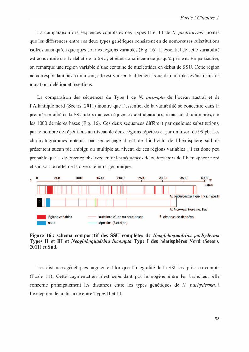
________________________________________________________________________Partie I Chapitre 2
98
La comparaison des séquences complètes des Types II et III de N. pachyderma montre
que les différences entre ces deux types génétiques consistent en de nombreuses substitutions
isolées ainsi qu’en quelques courtes régions variables (Fig. 16). L’essentiel de cette variabilité
est concentrée sur le début de la SSU, et était donc inconnue jusqu’à présent. En particulier,
on remarque une région variable d’une centaine de nucléotides en début de SSU. Cette région
ne correspondant pas à un insert, elle est vraisemblablement issue de multiples évènements de
mutation, délétion et insertions.
La comparaison des séquences du Type I de N. incompta de l’océan austral et de
l’Atlantique nord (Seears, 2011) montre que l’essentiel de la variabilité se concentre dans la
première moitié de la SSU alors que ces séquences sont identiques, à une substitution près, sur
les 1000 dernières bases (Fig. 16). Ces deux séquences diffèrent par quelques substitutions,
par le nombre de répétitions au niveau de deux régions répétées et par un insert de 93 pb. Les
chromatogrammes obtenus par séquençage direct de l’individu de l’hémisphère sud ne
présentent aucun pic ambigu ou multiple au niveau de ces régions variables ; il est donc peu
probable que la divergence observée entre les séquences de N. incompta de l’hémisphère nord
et sud soit le reflet de la diversité intra-génomique.
Figure 16 : schéma comparatif des SSU complètes de Neogloboquadrina pachyderma
Types II et III et Neogloboquadrina incompta Type I des hémisphères Nord (Seears,
2011) et Sud.
Les distances génétiques augmentent lorsque l’intégralité de la SSU est prise en compte
(Table 11). Cette augmentation n’est cependant pas homogène entre les branches : elle
concerne principalement les distances entre les types génétiques de N. pachyderma, à
l’exception de la distance entre Types II et III.
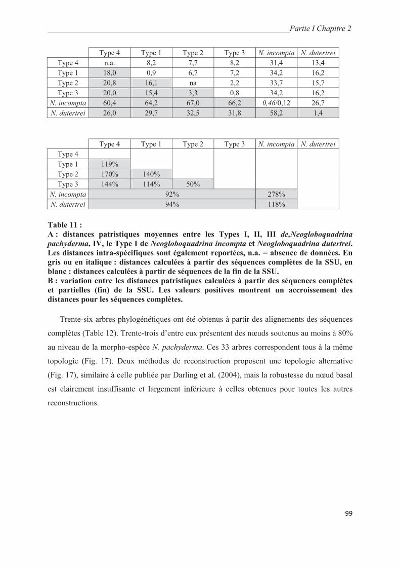
________________________________________________________________________Partie I Chapitre 2
99
Type 4 Type 1 Type 2 Type 3 N. incompta N. dutertrei
Type 4 n.a. 8,2 7,7 8,2 31,4 13,4
Type 1 18,0 0,9 6,7 7,2 34,2 16,2
Type 2 20,8 16,1 na 2,2 33,7 15,7
Type 3 20,0 15,4 3,3 0,8 34,2 16,2
N. incompta 60,4 64,2 67,0 66,2 0,46/0,12 26,7
N. dutertrei 26,0 29,7 32,5 31,8 58,2 1,4
Type 4 Type 1 Type 2 Type 3 N. incompta N. dutertrei
Type 4
Type 1 119%
Type 2 170% 140%
Type 3 144% 114% 50%
N. incompta 92% 278%
N. dutertrei 94% 118%
Table 11 :
A : distances patristiques moyennes entre les Types I, II, III de,Neogloboquadrina
pachyderma, IV, le Type I de Neogloboquadrina incompta et Neogloboquadrina dutertrei.
Les distances intra-spécifiques sont également reportées, n.a. = absence de données. En
gris ou en italique : distances calculées à partir des séquences complètes de la SSU, en
blanc : distances calculées à partir de séquences de la fin de la SSU.
B : variation entre les distances patristiques calculées à partir des séquences complètes
et partielles (fin) de la SSU. Les valeurs positives montrent un accroissement des
distances pour les séquences complètes.
Trente-six arbres phylogénétiques ont été obtenus à partir des alignements des séquences
complètes (Table 12). Trente-trois d’entre eux présentent des nœuds soutenus au moins à 80%
au niveau de la morpho-espèce N. pachyderma. Ces 33 arbres correspondent tous à la même
topologie (Fig. 17). Deux méthodes de reconstruction proposent une topologie alternative
(Fig. 17), similaire à celle publiée par Darling et al. (2004), mais la robustesse du nœud basal
est clairement insuffisante et largement inférieure à celles obtenues pour toutes les autres
reconstructions.

________________________________________________________________________Partie I Chapitre 2
100
Figure 17 : topologies obtenues pour différents modes de reconstruction phylogénétique
entre les séquences complètes des types génétiques de Neogloboquadrina pachyderma
(Table 12). Les longueurs de branches ne sont pas prises en compte. Les arbres sont
enracinés grâce aux outgroups (triangle rouge). La robustesse moyenne des nœuds (en
%) est reportée.
espèces alignement Gblock PHYML NJ BioNJ
Np+Nd
muscle x I/84 I/94 I/96
– I/80 I/91 I/89
mafft x I/93 I/99 I/99
– I/99 I/99 I/99
Np+Nd+Ni
muscle x I/53 II/54 II/68
– I/99 I/100 I/96
mafft x I/100 I/100 I/99
– I/100 I/100 I/100
Np+Nd+Po+Gi
muscle x I/97 I/92 I/91
– I/99 I/88 I/86
mafft x I/95 I/96 I/94
– I/97 I/98 I/97
Table 12 : topologies obtenues pour différents modes de reconstruction phylogénétique
entre les types génétiques de Neogloboquadrina pachyderma. I ou II se réfèrent aux
arbres de la figure 17, le nombre suivant représente la robustesse du nœud (en %) entre
le Type IV et le clade sub-antarctique. Espèces : groupes extérieurs utilisés ; Np + Nd :
N. pachyderma et Neogloboquadrina dutertrei ; Np+Nd+Ni : N. pachyderma, N. dutertrei,
Neogloboquadrina incompta ; Np+Nd+Po+Gi : N. pachyderma, N. dutertrei, Pulleniatina
obliquiloculata, Globoconella inflata.
________________________________________________________________________Partie I Chapitre 2
101
4. Discussion
4.1. Implications phylogénétiques
Lors de cette étude nous avons généré des arbres phylogénétiques à partir des
séquences de la fin de la SSU en utilisant des modèles se référant au maximum de
vraisemblance et au « neighbor-joining ». L’arbre obtenu par André et al. (en préparation A)
grâce à une méthode bayésienne est identique à l’un d’entre eux (Fig. 14, Table 10). Pourtant,
aucun de ces arbres phylogénétiques ne correspond à celui publié par Darling et al. (2007)
(Fig. 14). Ceci est d’autant plus étonnant que la phylogénie de Darling et al. (2007) est basée
sur ces mêmes modèles de reconstruction. Cette non-reproductibilité de l’arbre proposé par la
littérature est donc vraisemblablement due à des différences au niveau des alignements :
Darling et al. (2007) ont aligné les séquences manuellement alors que nous avons utilisé des
logiciels d’alignement automatique; or, la comparaison des arbres obtenus selon les
différentes méthodes a montré la sensibilité des reconstructions à la méthode d’alignement.
Les relations phylogénétiques entre les différents types génétiques de N. pachyderma basées
sur les séquences de la fin de la SSU sont donc très sensibles aux conditions analytiques (Fig.
14 ; Table 10) et on ne peut pas considérer cette phylogénie comme résolue de façon
satisfaisante.
Les reconstructions phylogénétiques basées sur les séquences complètes présentant
des nœuds suffisamment robustes (Table 12), validant le Type IV comme premier
embranchement au sein de N. pachyderma comme le suggéraient les arbres obtenus au cours
de cette étude à partir des séquences de la fin de la SSU (Fig. 14). De façon générale, on
remarque que les nœuds sont plus robustes avec les séquences complètes qu’avec les
séquences partielles. De plus, l’utilisation des séquences complètes augmente les distances
génétiques et donc l’information disponible pour les reconstructions phylogénétiques (Table
11). Cette augmentation est hétérogène entre les différentes branches, entrainant une
augmentation de la résolution phylogénétique au niveau de la morpho-espèce N. pachyderma
tout en limitant l’attraction des longues branches pour N. incompta. Ces premiers résultats
suggèrent donc que l’obtention de séquences complètes permettrait de résoudre les relations
phylogénétiques au sein de N. pachyderma. Néanmoins la diversité intra-génomique au
niveau de la SSU est encore pratiquement inconnue chez N. pachyderma et pourrait, si elle est
________________________________________________________________________Partie I Chapitre 2
102
conséquente, générer du bruit dans le signal phylogénétique, ce qui limiterait l’intérêt des
séquences longues.
4.2. Statut taxonomique des types génétiques de N. pachyderma et N. incompta
à partir de séquences complètes
La région la mieux connue de l’ADN ribosomal, la fin de la SSU, est aussi celle qui
présente le moins de variabilité (Fig. 15). Or, le statut taxonomique des types subantarctiques
qui présentent des séquences au niveau de la fin de la SSU peu divergentes, reste ambigu (Fig.
14 et André et al., en préparation A). Il semblerait donc judicieux d’utiliser des séquences
complètes de la SSU au lieu de séquences partielles afin d’inclure plus de variabilité, donc
d’information, pour résoudre la question du statut taxonomique de ces types génétiques. De
plus, la région utilisée correspondrait alors à l’unité complète sur laquelle jouent les processus
évolutifs, permettant ainsi de mieux estimer les distances génétiques, surtout entre espèces
proches.
Les séquences complètes des Types II et III de N. pachyderma (Fig. 16) montrent que la
divergence entre ces deux types génétiques a été sous-estimée d’environ 50 % (Table 11).
Néanmoins, ces données restent insuffisantes pour affirmer que les Types II et III sont bien
deux espèces distinctes. La présence d’une région variable conséquente (~100 pb) en début de
SSU semble en faveur de l’hypothèse de deux espèces différentes mais la divergence totale
entre les deux types génétiques reste globalement faible (3.3 %). Une étude de la diversité
intra-génomique et l’obtention de plus de séquences reste donc impérative pour valider le
statut taxonomique de ces deux types génétiques à l’aide de méthodes quantitatives (André et
al., en préparation A).
Des études précédentes (Darling et al., 2000, 2006 ; André et al., in prep A) ont montré,
sur la base de séquences de la fin de la SSU, que les N. incompta de l’hémisphère sud et celles
de l’Atlantique nord présentent des séquences largement identiques et correspondent donc à la
même espèce. Cependant, les séquences complètes montrent que la diversité génétique réelle
au sein de la SSU du Type I de N. incompta est presque 3 fois plus importante que celle
estimée à partir de séquences partielles. On remarque de plus une structuration nette de cette
variabilité en un insert et des répétitions (Fig. 16). Une structuration génétique Nord-Sud chez
N. incompta est donc envisageable. Les échanges génétiques entre les deux hémisphères
seraient donc plus sporadiques que ne l’envisageaient Darling et al. (2000). Néanmoins, la
________________________________________________________________________Partie I Chapitre 2
103
distance génétique totale au sein du type génétique reste faible (1.4 %) ce qui suggère qu’il ne
s’agirait pas d’espèces différentes. Ces observations nécessitent cependant d’être répliquées
sur un nombre plus important d’individus afin d’établir clairement si ces différences
génétiques sont systématiques et bien corrélées à la biogéographie.
4.3. Révision des scénarios phylogéographiques de N. pachyderma
Les relations phylogénétiques au sein de N. pachyderma ne sont pas totalement
résolues. En particulier, il est impossible de dégager un consensus sur les relations entre les
types génétiques au sein du clade formé par les N. pachyderma subantarctiques (Types II, III,
V et VI) (Fig. 14) qui présentent des séquences très peu divergentes (Table 11). De plus, les
données issues des séquences complètes et les données biogéographiques (André et al., en
préparation B) sont encore largement insuffisantes pour conclure quant au statut taxonomique
des Types II et III.
Si l’on se limite à l’étude des relations phylogénétiques entre les Types I, VI, VII et le
clade subantarctique, les résultats obtenus se résument à seulement deux types d’arbres
phylogénétiques (Fig. 18). Deux nouveaux scénarios évolutifs sont donc envisageables. Les
N. pachyderma ancestrales, vraisemblablement d’affinité sub-polaire à polaire, présentaient
une distribution bipolaire (Darling et al., 2004) mais avec un flux génétique efficace entre les
deux hémisphères (Darling et al., 2000 ; Finlay, 2002). La première spéciation correspond à
l’adaptation du Type IV aux conditions polaires extrêmes des eaux antarctiques à partir de ces
formes ancestrales. Ce premier embranchement est différent de celui proposé par Darling et
al. (2007), mais largement soutenu à la fois par les phylogénies basées sur la fin de la SSU et
les séquences complètes (Fig. 14 et 17). Une première spéciation au niveau de l’Antarctique
est plausible car au Pliocène (~4 Ma), des N. pachyderma sont déjà présentes à proximité du
continent antarctique en association avec des marqueurs d’un climat polaire (Pattersson et
Ishman, 2012). Les occurrences plus anciennes de N. pachyderma restent sujettes à caution en
raison de sa grande proximité morphologique avec l’espèce fossile Neogloboquadrina
acostaensis pouvant entrainer des attributions taxonomiques erronées (Kennett et Srinivasan,
1983 ; Loubere et Moss, 1986). Plus tardivement, les échanges génétiques entre les deux
hémisphères ont été rompus. D’après le registre fossile, on peut estimer la date de cet
évènement à ~1 Ma, date qui correspond à l’apparition de N. pachyderma d’affinités
clairement polaires dans l’Atlantique nord (par exemple Speigler et Jansen, 1989 ; Huber et
________________________________________________________________________Partie I Chapitre 2
104
al., 2000). Cette rupture du flux génétique coïncide avec l’intensification des périodes
glaciaires liée au début de la périodicité de 100 ka des cycles glaciaires (Mudelsee et Schulz,
1997). Ces changements climatiques auraient entrainé une adaptation aux eaux polaires des N.
pachyderma de l’hémisphère nord. Selon le scénario A (Fig. 17), cette rupture est synchrone
entre océans Atlantique et Pacifique. L’étude de Kucera et Kennett (2002) basée sur des
arguments morphologiques et géochimiques semblerait valider cette hypothèse : les auteurs
ont conclu à l’apparition des N. pachyderma modernes vers 1 Ma de façon synchrone entre
océans Atlantique et Pacifique. Selon le scénario B (Fig. 16), la rupture du flux génétique a
d’abord eu lieu au niveau de l’océan Atlantique suite à l’adaptation aux environnements
polaires du Type I. Cette hypothèse reste plausible car le début des glaciations dans
l’Atlantique nord a entrainé la mise en place d’un domaine polaire (Mudelsee et Schulz,
1997). De plus, la présence du Gulf Stream et de la dérive nord Atlantique peuvent être une
barrière au transit entre hémisphère nord et sud pour des espèces d’eaux froides (Darling et
al., 2004). Au contraire, le flux génétique entre Pacifique nord et sud a pu se maintenir plus
longtemps notamment du fait de l’absence de domaine véritablement polaire dans cette région
(Lipps, 1972) et de la présence de longs upwellings côtiers pouvant servir de zone de transit
pour les N. pachyderma (Darling et al., 2004).
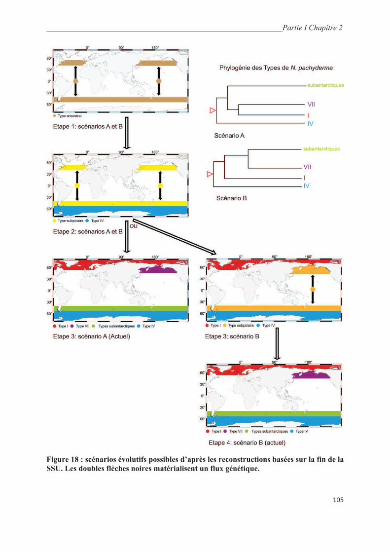
________________________________________________________________________Partie I Chapitre 2
105
Figure 18 : scénarios évolutifs possibles d’après les reconstructions basées sur la fin de la
SSU. Les doubles flèches noires matérialisent un flux génétique.

________________________________________________________________________Partie I Chapitre 2
106
5. Conclusions
La phylogénie des types génétiques de Neogloboquadrina pachyderma, basée sur les
1000 dernières bases de la SSU, n’est pas suffisamment résolue ce qui limite la
compréhension de l’histoire évolutive de cette morpho-espèce. Malgré une forte influence des
méthodes employées sur la topologie des arbres phylogénétiques, quelques points constants
ressortent comme le fait que la première spéciation soit liée à l’adaptation du Type IV aux
conditions polaires extrêmes de l’Antarctique. La rupture du flux génétique entre les deux
hémisphères est plus tardive et probablement concomitante à la mise en place des cycles
glaciaire-interglaciaires de 100 ka. Une phylogénie plus robuste permettrait 1) de déterminer
si la rupture du flux génétique a été synchrone entre les océans Pacifique et Atlantique, et 2)
de déterminer le nombre d’espèces présentes au sein du clade formé par les N. pachyderma
subantarctiques (Types II, III, V, VI).
Les premières séquences complètes de la SSU des Types I, II, III et IV de N.
pachyderma et de Neogloboquadrina incompta montrent que le début de la SSU chez ces
morpho-espèces comporte de longues régions variables alors que la fin de la SSU concentre
de nombreuses régions conservées, ce qui pourrait expliquer la difficulté d’obtenir une
reconstruction phylogénétique satisfaisante à partir de cette dernière région. L’utilisation des
séquences complètes, qui incluent plus de variabilité, semble donc une solution prometteuse
pour établir une phylogénie plus robuste d’autant plus que les premières séquences complètes
obtenues valident la position phylogénétique du Type IV comme premier embranchement. La
comparaison des séquences complètes des Types II et III suggère que ces deux types
génétiques sont potentiellement deux espèces différentes et la comparaison des Types I de N.
incompta des hémisphères nord et sud suggère une structuration nord-sud chez ce type
génétique. Cette étude nécessite néanmoins d’être approfondie par l’ajout de séquences en
provenance de tous les types génétiques connus de N. pachyderma (notamment le Type VII)
et par le séquençage de clones afin d’évaluer la diversité intra-génomique. Même si
l’obtention de séquences complètes reste fastidieuse notamment du fait de la grande longueur
de la SSU chez les foraminifères planctoniques, l’obtention de séquences complètes devrait
permettre de résoudre la question du statut taxonomique des types génétiques et de leurs
relations phylogénétiques.
________________________________________________________________________Partie I Chapitre 2
107
Remerciements
Je remercie Lara Konecny pour son assistance technique. Je remercie également
Elisabeth Michel qui a récolté les échantillons lors de la campagne OISO-21, l’équipage et les
équipes scientifiques du Marion-Dufresne ainsi que l’Institut Polaire Paul-Emile Victor
(IPEV). Ce travail a pu être réalisé grâce au financement de l’Institut National des Sciences
de l’Univers (INSU), programme INTERRVIE (F.Q.).
Supplément
Séquences complètes et alignements utilisés pour les reconstructions phylogénétiques
____________________________________________________________Partie I Chapitre 2
108
Références
Akaike, H., 1974. A new look at the statistical model identification. Institute of Electrical and
Electronics Engineers Transactions on Automatic Control, 19: 716-723.
André, A., Weiner, A., Quillévéré, F., Aurahs, R., Morard, R., Douady, C., de Garidel-
Thoron, T., Escarguel, G., de Vargas, C. and Kucera, M., 2013. The cryptic and the
apparent reversed: lack of genetic differentiation within the morphologically diverse
plexus of the planktonic foraminifer Globigerinoides sacculifer. Paleobiology, 39: 21-
39.
André, A., Quillévéré, F., Morard, R., de Vargas, C., Ujiié, Y., and Douady, C., in prep. A.
SSU rDNA divergence in planktonic foraminifera: molecular taxonomy and
biogeographic implications.
André, A., Quillévéré, F., Escarguel, G., Michel, E. and Douady, C., in prep. B. A case of true
cryptic species within planktonic foraminifera: eco-phenotypic morphological variations
of Southern Ocean Neogloboquadrina pachyderma genetic types.
Aurahs, R., Göker, M., Grimm, G., Hemleben, V., Hemleben, C., Schiebel, R. and Kucera,
M., 2009. Using the multiple analysis approach to reconstruct phylogenetic
relationships among planktonic foraminifera from highly divergent and length-
polymorphic SSU rDNA sequences. Bioinformatics and Biology Insights, 3: 155-177.
Bartoli, G., Sarnthien, M., Weinelt, M., Erlenkeuser, H., Garbe-Schonberg, D. and Lea, D.,
2005. Final closure of Panama and the onset of northern hemisphere glaciation. Earth
and Planetary Science letters, 237: 33-44.
Becquey, S. and Gersonde, R., 2003. A 0.55-Ma paleotemperature record from the
subantarctic zone: implications for Antarctic Circumpolar Current development.
Paleoceanography, 18: 1014-1028.
Castresana, J., 2000. Selection of conserved blocks from multiple alignments for their use in
phylogenetic analysis. Molecular Biology and Evolution, 17: 540-552.
Darling, K.F., Wade, C.M., Stewart, I.A., Kroon, D., Dingle R. and Brown, A.J., 2000.
Molecular evidence for genetic mixing of Arctic and Antarctic subpolar populations of
planktonic foraminifers. Nature, 405: 43-47.
Darling, K.F., Kucera, M., Wade, C.M., Langen, P.V. and Pak, D., 2003. Seasonal
distribution of genetic types of planktonic foraminifer morphospecies in the Santa
Barbara Channel and its paleoceanographic implications. Paleoceanography, 18: 1032-
1042.
Darling, K.F., Kucera, M., Pudsey, C.J. and Wade, C.M., 2004. Molecular evidence links
cryptic diversification in polar planktonic protists to Quaternary climate dynamics.
Proceedings of the National Academy of Science of the United States of America, 101:
7657-7662.
Darling, K.F., Kucera, M., Kroon, D. and Wade, C.M., 2006. A resolution for the coiling
direction paradox in Neogloboquadrina pachyderma. Paleoceanography, 21: 1-14.
____________________________________________________________Partie I Chapitre 2
109
Darling, K.F., Kucera, M. and Wade, C.M., 2007. Global molecular phylogeography reveals
persistent arctic circumpolar isolation in a marine planktonic protist. Proceedings of the
National Academy of Science of the United States of America, 104: 5002-5007.
Darling, K.F. and Wade, C.M., 2008. The genetic diversity of planktic foraminifera and the
global distribution of ribosomal RNA genotypes. Marine Micropaleontology, 67: 216-
238.
de Vargas, C., Zaninetti, L., Hilbrecht, H. and Pawlowski, J., 1997. Phylogeny and rates of
molecular evolution of planktonic foraminifera: SSU rDNA sequences compared to the
fossil record. Journal of Molecular Evolution, 45: 285-294.
Edgar, R.C., 2004. MUSCLE: multiple sequence alignment with high accuracy and high
throughput. Nucleic Acids Research, 32: 1792-1797.
Ertan, K.T., Hemleben, V. and Hemleben, C., 2004. Molecular evolution of some selected
benthic foraminifera as inferred from sequences of the small subunit ribosomal DNA.
Marine Micropaleontology, 53: 367-388.
Finlay, B.J., 2002. Global dispersal of free-living microbial eukaryote species. Science, 296:
1061-1063.
Gascuel, O., 1997. BIONJ: an improved version of the NJ algorithm based on a simple model
of sequence data. Molecular Biology and Evolution, 14: 685-695.
Gast, R.J. and Caron, D.A., 1996. Molecular phylogeny of symbiotic dinoflagellates from
planktonic foraminifera and radiolaria. Molecular Biology and Evolution, 13: 1192-
1197.
Gouy, M., Guindon, S.P. and Gascuel, O., 2010. SeaView Version 4: a multiplatform
graphical user interface for sequence alignment and phylogenetic tree building.
Molecular Biology and Evolution, 27: 221-224.
Guindon, S. and Gascuel, O., 2003. A simple, fast, and accurate algorithm to estimate large
phylogenies by maximum likelihood. Systematic Biology, 52:696-704.
Huber, R., Meggers, H., Baumann, K.-H., Raymo, M.E. and Henrich, R., 2000. Shell size
variation of the planktonic foraminifer Neogloboquadrina pachyderma sin. in the
Norwegian-Greenland Sea during the last 1.3 Myrs: implications for paleoceanographic
reconstructions. Palaeogeography, Palaeoclimatology, Palaeoecology, 160: 193-212.
Katoh, K. and Toh, H., 2008. Recent developments in the MAFFT multiple sequence
alignment program. Briefings in Bioinformatics, 9: 276-285.
Kennett, J.P. and Srinivasan, M.S., 1983. Neogene Planktonic Foraminifera: a Phylogenetic
Atlas. Hutchinson Ross, Sroudsburg (Pennsylvania).
Kucera, M. and Darling, K.F., 2002. Cryptic species of planktonic foraminifera: their effect
on palaeoceanographic reconstructions. Philosophical Transaction of the Royal Society
of London, 360: 695-718.
Kucera, M. and Kennett, J.P., 2002. Causes and consequences of a middle Pleistocene origin
of the modern planktonic foraminifer Neogloboquadrina pachyderma sinistral.
Geology, 30: 539-542.
Lipps, J.H., 1972. Plankton biostratigraphy and paleoecology of the Eastern North Pacific
Ocean: introduction. Palaeogeography, Palaeoclimatology, Palaeoecology, 12: 3-14.
____________________________________________________________Partie I Chapitre 2
110
Loubere, P. and Moss, K., 1986. Pliocene climatic change and the onset of the Northern
Hemisphere glaciation as recorded in the northeast Atlantic Ocean. Geological Society
of America Bulletin, 97: 818-828.
MARGO project members, 2009. Constraints on the magnitude and patterns of ocean cooling
at the last glacial maximum. Nature Geoscience, 2: 127-132.
Morard, R., Quillevere, F., Escarguel, G., de Garidel-Thoron, T., de Vargas, C. and Kucera,
M., 2013. Ecological modeling of the temperature dependence of cryptic species of
planktonic foraminifera in the Southern Hemisphere. Palaeogeography
Palaeoclimatology Palaeoecology. http://dx.doi.org/10.1016/j.palaeo.2013.05.011
Mudelsee, M. and Schulz, M., 1997. The Mid-Pleistocene climate transition: onset of 100 ka
cycle lags ice volume build-up by 280 ka. Earth and Planetary Science Letters, 151:
117-123.
Paradis, E., Claude, J. and Strimmer, K., 2004. APE: analyses of phylogenetics and evolution
in R language. Bioinformatics, 20: 289-290.
Patterson, M.O. and Ishman, S.E., 2012. Neogene benthic foraminiferal assemblages and
paleoenvironmental record for McMurdo Sound, Antarctica. Geosphere, 8: 1331-1341.
Pawlowski, J., Bolivar, I., Fahrni, J.F., Cavalier-Smith, T. and Gouy, M., 1996. Early origin
of foraminifera suggested by SSU rRNA gene sequences. Molecular Biology and
Evolution, 13: 445-450.
Posada, D. and Crandall, K.A., 1998. Modeltest: testing the model of DNA substitution.
Bioinformatics, 14: 817-818.
R Development Core Team, 2004. R: a language and environment for statistical computing.
Saitou, N. and Nei, M., 1987. The neighbor-joining method: a new method for reconstructing
phylogenetic trees. Molecular Biology and Evolution, 4: 406-425.
Schweizer, M., Pawlowski, J., Kouwenhoven, T.J., Guiard, J. and van der Zwaan, B., 2008.
Molecular phylogeny of Rotaliida (Foraminifera) based on complete small subunit
rDNA sequences. Marine Micropaleontology, 66: 233-246.
Seears, H., 2011. Biogeography and phylogenetics of the planktonic foraminifera. PhD
Thesis. University of Nottingham.
Smith, L.M., Sanders, J., Kaiser, R., Hughes, P., Dodd, C., Connell, C., Heiner, C., Kent, S.
and Hood, L., 1986. Fluorescence detection in automated DNA sequence analysis.
Nature, 321: 674-679.
Spiegler, D. and Jansen, E., 1989. Planktonic foraminifer biostratigraphy of Norwegian Sea
sediments: ODP LEG 104. Proceedings of the Ocean Drilling Program, Scientific
Results, 104: 681-696.
Studier, J.A. and Keppler, K.J., 1988. A note on the neighbor-joining algorithm of Saitou and
Nei. Molecular Biology and Evolution, 5: 729-731.
Ufkes, E., Jansen, J.H.F. and Schneider, R.R., 2000. Anomalous occurrences of
Neogloboquadrina pachyderma (left) in a 420-ky upwelling record from Walvis Ridge
(SE Atlantic). Marine Micropaleontology, 40: 23-42.

____________________________________________________________Partie I Chapitre 2
111
Ujiie, Y. and Lipps, J.H., 2009. Cryptic diversity in planktic foraminifera in the northwest
Pacific Ocean. Journal of Foraminiferal Research, 39: 145-154.
Ujiié, Y., de Garidel-Thoron, T., Watanabe, S., Wiebe, P. and de Vargas, C., 2010. Coiling
dimorphism within a genetic type of the planktonic foraminifer Globorotalia
truncatulinoides. Marine Micropaleontology, 77: 145-153.
Weiner, A., Aurahs, R., Kurasawa, A., Kitazato, H. and Kucera, M., 2012. Vertical niche
partitioning between cryptic sibling species of a cosmopolitan marine planktonic protist.
Molecular Ecology, 21: 4063-4073.
White, T.J., Bruns, T., Lee, S. and Taylor, J.W., 1990. Amplification and direct sequencing of
fungal ribosomal RNA genes for phylogenetics. PCR Protocols: A Guide to Methods
and Applications, Academic Press, New York.

112
PARTIE II
TAXONOMIES MORPHOLOGIQUE ET
MOLECULAIRE
CAS DE Globigerinoides sacculifer ET
Neogloboquadrina pachyderma

_______________________________________________________________________Partie II Chapitre 1
113
Chapitre 1 : Un cas particulier, Globigerinoides
sacculifer, morpho-espèce présentant une forte
diversité morphologique associée à une très faible
diversité génétique
De par sa vaste distribution géographique, ses larges affinités environnementales et sa
grande diversité morphologique, il était attendu que Globigerinoides sacculifer corresponde
au regroupement de plusieurs espèces cryptiques. Les séquences de la fin de la SSU et de
l’ITS-1 obtenues à partir d’un échantillonnage à l’échelle mondiale montrent, au contraire,
une diversité génétique très réduite chez cette morpho-espèce. La méthode d’extraction de
l’ADN employée étant non destructrice, une absence de relation entre distance génétique et
type morphologique a pu être mise en évidence. Globigerinoides sacculifer correspond donc à
une unique espèce et est le premier cas chez les foraminifères planctoniques où la diversité
morphologique d’une morpho-espèce est supérieure à sa diversité génétique.
Cette absence de diversité génétique est d’autant plus étonnante que G. sacculifer est une
espèce ancienne (~ 19 Ma) et que les populations atlantiques sont pratiquement isolées de
celles des océans indiens et pacifiques. La présence d’un haplotype de l’ITS-1 spécifique à
l’océan atlantique suggère que les G. sacculifer de l’océan atlantique ont été récemment
(dernier maximum glaciaire) isolés puis qu’un flux génétique unidirectionnel de l’océan
indien vers l’atlantique s’est rétabli.
Mots-clefs : Globigerinoides sacculifer, Globigerinoides trilobus, Globigerinoides
quadrilobatus, Globigerinoides sacculifer immaturus, SSU, ITS-1, diversité génétique, flux
génétique unidirectionnel
Fiches-méthode (annexe) : I, III, IV, V, VII, VIII
Ce manuscrit a été publié dans la revue Paleobiology en Janvier 2013

_______________________________________________________________________Partie II Chapitre 1
114
The cryptic and the apparent reversed: lack of genetic
differentiation within the morphologically diverse plexus of the
planktonic foraminifer Globigerinoides sacculifer
Aurore Andréa, Agnes Weiner
b, Frédéric Quillévéré
a, Ralf Aurahs
b, Raphaël Morard
c,
Christophe J. Douadyd, Thibault de Garidel-Thoron
e, Gilles Escarguel
a, Colomban de Vargas
c,
Michal Kucerab
a UMR CNRS 5276, Laboratoire de Géologie de Lyon: Terre, Planètes, Environnement,
Université Lyon 1, 27-43 Boulevard du 11 Novembre 1918, 69622 Villeurbanne Cedex,
France
b Zentrum für marine Umweltwissenschaften MARUM, Universität Bremen, Leobener
Strasse, 28359 Bremen, Germany
c UMR CNRS 7144, Evolution du Plancton et PaléoOcéans, UPMC Université Paris 06,
Station Biologique, BP 74, 29682 Roscoff, France
d UMR5023, Ecologie des Hydrosystèmes Naturels et Anthropisés, Université Lyon 1,
ENTPE, CNRS, 6 rue Raphaël Dubois, 69622 Villeurbanne, France
e CEREGE UMR 6635, Université Aix-Marseille, 13545 Aix-en-Provence Cedex 4, France

_______________________________________________________________________Partie II Chapitre 1
115
Abstract
Previous genetic studies of extant planktonic foraminifera have provided evidence that the
traditional, strictly morphological definition of species in these organisms underestimates
their biodiversity. Here, we report the first case where this pattern is reversed. The modern
(sub)tropical species plexus Globigerinoides sacculifer is characterized by large
morphological variability, which has led to the proliferation of taxonomic names attributed to
morphological end-members within the plexus. In order to clarify the taxonomic status of its
morphotypes and to investigate the genetic connectivity among its currently partly disjunct
(sub)tropical populations, we carried out a global survey of two ribosomal RNA regions (SSU
and ITS-1) in all recent morphotypes of the plexus collected throughout (sub)tropical surface
waters of the global ocean. Unexpectedly, we find an extremely reduced genetic variation
within the plexus and no correlation between genetic and morphological divergence,
suggesting taxonomical overinterpretation. The genetic homogeneity within the
morphospecies is unexpected, considering its partly disjunct range in the (sub)tropical
=Atlantic and Indo-Pacific and its old age (early Miocene). A sequence variant in the rapidly
evolving ITS-1 region indicates the existence of an exclusively Atlantic haplotype, which
suggests an episode of relatively recent (last glacial) isolation, followed by subsequent
resumption of unidirectional gene flow from the Indo-Pacific into the Atlantic. This is the first
example in planktonic foraminifera where the morphological variability in a morphospecies
exceeds its rDNA genetic variability. Such evidence for inconsistent scaling of morphological
and genetic diversity in planktonic foraminifera could complicate the interpretation of
evolutionary patterns in their fossil record.
Keywords: Globigerinoides sacculifer, Globigerinoides trilobus, Globigerinoides
quadrilobatus, Globigerinoides sacculifer immaturus, SSU, ITS-1, genetic diversity,
unidirectional gene flow

_______________________________________________________________________Partie II Chapitre 1
116
1. Introduction
The interpretation of biogeographical and evolutionary patterns of morphologically
defined species in the plankton has been challenged by the discovery of cryptic genetic
diversity often linked with distinct biogeography and ecological adaptation (e.g., Saez et al.
2003; Logares et al. 2007; Kooistra et al. 2008). The interpretation of modern and fossil
species distribution patterns in these groups thus hinges on the degree of congruence between
their morphological and genetic divergence. As long as the morphological taxonomy
consistently underestimates biodiversity, analysis of the fossil record and modern assemblages
may be expected to reflect processes scaled with those at the level of biological species. This
issue is particularly important for the interpretation of diversity patterns in the fossil record,
because the species concept in palaeontology (and in many cases in biology as well) is based
solely on phenotypic traits manifested in the shape of the classified organisms.
Planktonic foraminifera provide an excellent opportunity to test the explanatory power
of biogeographical and evolutionary patterns derived from morphologically defined species
and to assess the degree of congruence between morphological distinction and genetic
divergence. Their character-rich calcite shells are abundantly preserved in marine sediments
and allow direct tracking of morphospecies occurrences in time and space (e.g., Aze et al.
2011). From these occurrences, paleoceanographers derive reconstructions that are of
immense importance to our understanding of past climate changes. In recent years, molecular
analyses have revealed that the classical, morphological definition of species in planktonic
foraminifera hides cryptic genetic and ecological differentiation (for a review see Darling and
Wade 2008). Global surveys of the Small Subunit (SSU) or Internal Transcribed Spacers
(ITS) regions of ribosomal DNA (rDNA) in extant species allowed the recognition of distinct
genotypes(e.g., de Vargas et al. 1999, 2001; Darling et al. 1999, 2006; Morard et al. 2009,
2011; Ujiié et al. 2010; Aurahs et al. 2011; Quillévéré et al. 2012). Considering the lack of
evidence for introgression and the obligate sexual outbreeding reproductive modus in
planktonic foraminifera, these genetic types have to be considered reproductively isolated and
thus corresponding at least to the level of biological species. Many of these genetic types
show more restricted biogeographical ranges than the morphospecies to which they have been
assigned, implying that the distribution of these morphospecies does not reflect the true
potential for dispersal of these organisms. Nonetheless, some of these genetic types occur
throughout the range of their respective morphospecies, suggesting ongoing global gene flow.
_______________________________________________________________________Partie II Chapitre 1
117
At present, the degree to which morphological divergence reflects genetic distinction in
planktonic foraminifera (and potentially other plankton) remains unclear, complicating the
interpretation of biogeographical and evolutionary patterns in the fossil record of this group.
Here we report on a global survey of two of the ribosomal rDNA regions (SSU and
ITS-1) in the abundant and paleoceanographically important (sub)tropical species
Globigerinoides sacculifer (Brady 1877). The survey was carried out with the aim to
determine the degree of congruence between morphology and genetic divergence within this
morphologically diverse species plexus, and to investigate the genetic connectivity among its
partly disjunct (sub)tropical populations. Globigerinoides sacculifer is one of the most
commonly encountered planktonic foraminifera in the (sub)tropical waters of the world
oceans (e.g., Tolderlund and Bé 1971). This cosmopolitan spinose species is limited by its
photosymbiotic ecology to the euphotic zone of the oceans, where it reproduces on a synodic
lunar cycle (Bijma et al. 1990).
The morphology associated with the species concept of Globigerinoides sacculifer
initially occurred during the early Miocene ~20 Myr ago, having diverged from the
morphospecies Globigerinoides trilobus (e.g., Kennett and Srinivasan 1983; Berggren et al.
1995). The exact dating of this divergence is potentially complicated by usage of the species
names G. sacculifer and G. trilobus in a way not consistent with their original species
description. Similarly, the taxonomic status of G. sacculifer in the modern ocean is
ambiguous, because of a high morphological variability among specimens of this plexus.
Globigerinoides sacculifer sensu stricto has been taxonomically distinguished from other
Globigerinoides morphospecies with a honeycomb shell wall texture (Kennett and Srinivasan
1983) by the presence of a sac-like final chamber (Brady 1877). Whereas the other taxonomic
concepts in the plexus (Fig. 19), Globigerinoides quadrilobatus (d’Orbigny 1846), G. trilobus
(Reuss 1850) and Globigerinoides immaturus Leroy (1939), are based on fossil material, G.
sacculifer was originally described from subfossil sediments and the original species
description clearly refers to the occurrence and habitat of this species in the plankton (Brady
1877; see also Williams et al. 2006). Numerous studies have noticed that the shells of G.
trilobus, G. quadrilobatus, and G. immaturus are virtually identical to those of G. sacculifer
except for the lack of the final sac-like chamber (Hofker 1959; Banner and Blow 1960; Hecht
1974; Saito et al. 1981). As a consequence, these taxa were often considered phenotypic
variants of the morphospecies G. sacculifer s.l. Culture experiments have provided support for
this broader taxonomic concept, suggesting that the sac-like chamber is probably a terminal
event of shell growth, manifested in some but not all of the cultured specimens (Bé 1980; Bé
_______________________________________________________________________Partie II Chapitre 1
118
et al. 1983; Hemleben et al. 1987; Bijma et al. 1992). Despite these culturing experiments,
specimens with and without the sac-like last chamber have been continually recorded as
separate taxa for paleoecological studies and transfer functions. Today, the most extensively
used species names for members of the plexus are G. trilobus and G. sacculifer, but G.
quadrilobatus and G. immaturus are still commonly reported, even in late Quaternary
sediments (e.g., Spooner et al. 2005; Lim et al. 2006; Budillon et al. 2009; Siani et al. 2010;
Wilson 2012).
Until now, only 16 SSU sequences of the Globigerinoides sacculifer plexus have been
published, 11 originating from a single location in the NW Pacific and the five remaining
originating from the South Pacific (Coral Sea), Atlantic (Caribbean Sea) and Mediterranean
(Wade et al. 1996; Darling et al. 1997; de Vargas et al. 1997; Pawlowski et al. 1997; Ujiié and
Lipps 2009). All these sequences were attributed to G. sacculifer. These sequences are
virtually identical, but the available data are not sufficient to address the global diversification
or to resolve the correlation between morphological and genetic divergence in the plexus.
Here, we assess the rDNA genetic diversity of the SSU and ITS regions from the G. sacculifer
plexus throughout the world oceans. Single-cell DNA analyses are performed on 148
individuals representative of all major morphotypes, i.e., Globigerinoides trilobus, G.
immaturus, G. quadrilobatus, and G. sacculifer s.s. (Fig. 19). Such analyses allow us to
determine whether or not there is cryptic diversity in G. sacculifer s.l. and to investigate the
congruence between genetic and morphological diversity within the plexus.
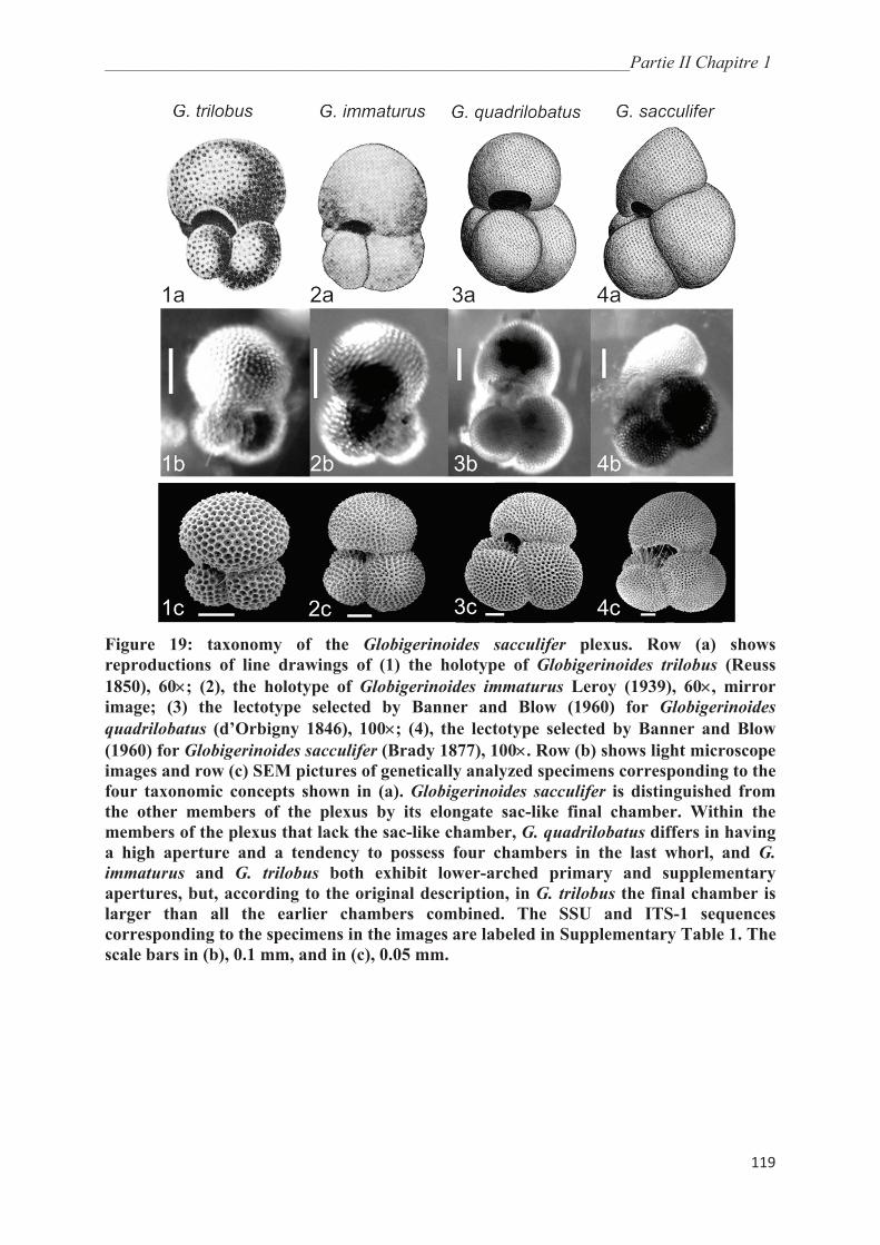
_______________________________________________________________________Partie II Chapitre 1
119
Figure 19: taxonomy of the Globigerinoides sacculifer plexus. Row (a) shows
reproductions of line drawings of (1) the holotype of Globigerinoides trilobus (Reuss
1850), 60 ; (2), the holotype of Globigerinoides immaturus Leroy (1939), 60 , mirror
image; (3) the lectotype selected by Banner and Blow (1960) for Globigerinoides
quadrilobatus (d’Orbigny 1846), 100 ; (4), the lectotype selected by Banner and Blow
(1960) for Globigerinoides sacculifer (Brady 1877), 100 . Row (b) shows light microscope
images and row (c) SEM pictures of genetically analyzed specimens corresponding to the
four taxonomic concepts shown in (a). Globigerinoides sacculifer is distinguished from
the other members of the plexus by its elongate sac-like final chamber. Within the
members of the plexus that lack the sac-like chamber, G. quadrilobatus differs in having
a high aperture and a tendency to possess four chambers in the last whorl, and G.
immaturus and G. trilobus both exhibit lower-arched primary and supplementary
apertures, but, according to the original description, in G. trilobus the final chamber is
larger than all the earlier chambers combined. The SSU and ITS-1 sequences
corresponding to the specimens in the images are labeled in Supplementary Table 1. The
scale bars in (b), 0.1 mm, and in (c), 0.05 mm.

_______________________________________________________________________Partie II Chapitre 1
120
2. Material and Methods
2.1. Sampling
Specimens of Globigerinoides sacculifer, G. immaturus, G. trilobus, and G.
quadrilobatus were collected from ring and stratified plankton tows (64- m to 200- m mesh
sizes) and by pumping surface water through a sieve with 64-μm mesh size (see Table 13 for
details). The sampling cruises took place from 1995 to 2010 and covered almost the entire
geographic range reported for G. sacculifer (Fig. 20). Right after sampling, live specimens
were taxonomically identified, in most cases photographed and carefully picked from the
plankton, cleaned with a fine brush, and transferred individually into a DNA extraction buffer.
Specimens were then stored at -20°C until further processing in the laboratory. Hydrographic
vertical profiles of the water column were obtained at most stations of collection by using
temperature and fluorescence sensors (Table 13).
Figure 20: location of ship tracks, names of the various cruises, and sampling stations
for individuals of the Globigerinoides sacculifer plexus. Black circles represent stations
where both SSU and ITS-1 sequences have been obtained; white circles represent
stations where only the SSU has been sequenced; open circles mark stations were only
the ITS-1 has been sequenced. Details of all localities are given in Table 13. Colours
indicate the relative abundance of the G. sacculifer plexus in planktonic foraminiferal
assemblages from surface sediments, interpolated from data in the MARGO database
(Kucera et al. 2005; MARGO Project Members 2009) and Siccha et al. (2009).
Table 13: Location of the sampling stations for Globigerinoides sacculifer with
hydrographic data, collection and DNA extraction methods, numbers of sequenced
individuals and, in the case of stations with cloned specimens or replicates, numbers of
sequences (in italic). Data from the literature are also included. Numbers in brackets
correspond to Orbulina universa ITS-1 sequences.
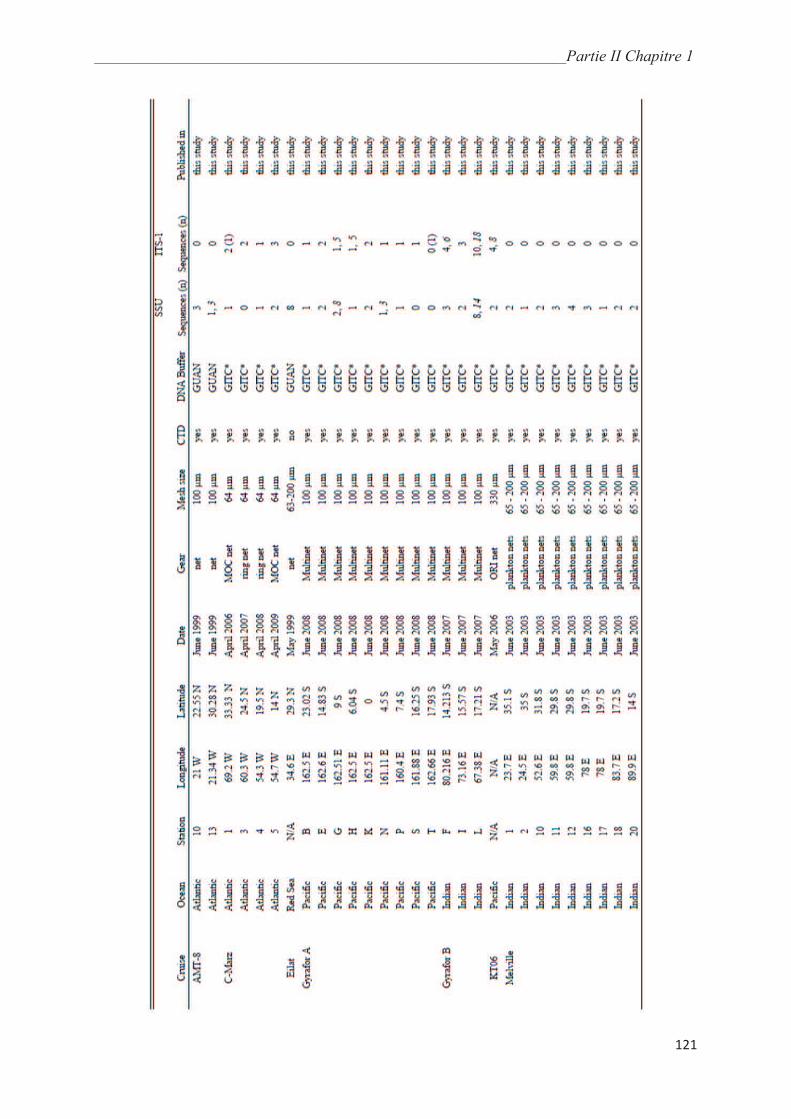
_______________________________________________________________________Partie II Chapitre 1
121
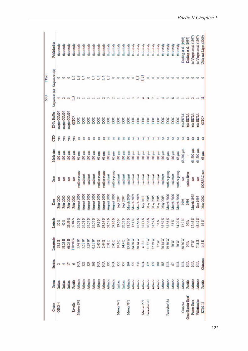
_______________________________________________________________________Partie II Chapitre 1
122
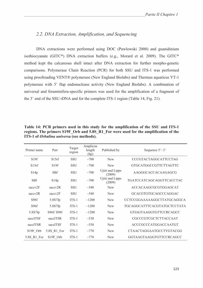
_______________________________________________________________________Partie II Chapitre 1
123
2.2. DNA Extraction, Amplification, and Sequencing
DNA extractions were performed using DOC (Pawlowski 2000) and guanidinium
isothiocyanate (GITC*) DNA extraction buffers (e.g., Morard et al. 2009). The GITC*
method kept the calcareous shell intact after DNA extraction for further morpho-genetic
comparisons. Polymerase Chain Reaction (PCR) for both SSU and ITS-1 was performed
using proofreading VENT® polymerase (New England Biolabs) and Thermus aquaticus YT-1
polymerase with 5’ flap endonuclease activity (New England Biolabs). A combination of
universal and foraminifera-specific primers was used for the amplification of a fragment of
the 3’ end of the SSU rDNA and for the complete ITS-1 region (Table 14, Fig. 21).
Table 14: PCR primers used in this study for the amplification of the SSU and ITS-1
regions. The primers S19F_Orb and 5.8S_R1_For were used for the amplification of the
ITS-1 of Orbulina universa (see methods).
Primer name Pair Target
region
Amplicon
length
(bp)
Published by Sequence 5’- 3’
S19f S15rf SSU ~700 New CCCGTACTAGGCATTCCTAG
S15rf S19f SSU ~700 New GTGCATGGCCGTTCTTAGTTC
S14p SBf SSU ~700 Ujiié and Lipps
(2009) AAGGGCACCACAAGAGCG
SBf S14p SSU ~700 Ujiié and Lipps
(2009) TGATCCATCAGCAGGTTCACCTAC
saccv2F saccv2R SSU ~540 New ACCACAAGCGCGTGGAGCAT
saccv2R saccv2F SSU ~540 New GCACGTGTGCAGCCCAGGAC
S98f 5.8S7fp ITS-1 ~1200 New CCTCCGGAAAAAGGCTTATGCAGGCA
S96f 5.8S7fp ITS-1 ~1200 New TGCAGGCATTTCACGTATGCTCCTATA
5.8S7fp S96f/ S98f ITS-1 ~1200 New GTIAGTAAGGTGTTCCRCAGCC
saccITSF saccITSR ITS-1 ~530 New CGCCCGTCGCTCTTACCAAT
saccITSR saccITSF ITS-1 ~530 New ACCCGCCCATGGACCAATGT
S19F_Orb 5.8S_R1_For ITS-1 ~770 New CTAACTAGGAATGCCTYGTACGG
5.8S_R1_For S19F_Orb ITS-1 ~770 New GGTAAGTAAGGTGTTCCRCAGCC

_______________________________________________________________________Partie II Chapitre 1
124
Figure 21: scheme of the SSU, ITS-1, and 5.8S regions of the planktonic foraminiferal
rRNA genes showing the positions of the amplified regions with appropriate primer
pairs (gray lines) for Globigerinoides sacculifer. Variable and conserved regions are
shown in white and black, respectively. The gray region shows the position of the insert
found in specimens of G. sacculifer s.l. from the Atlantic Ocean. Neogloboquadrina
dutertrei (NCBI EU199449) is taken as reference for SSU 5’ end length (in pair base).
SSU 3’ end, ITS-1, and 5.8S lengths are based on sequences of G. sacculifer.
The use of multiple primer pairs that were developed in the course of the project helped us to
improve the amplification success rates (e.g., from 44% to 70% for the SSU). The reason for
obtaining sequences of the ITS-1 region was the observation from species of non-spinose
planktonic foraminifera in which this region showed higher rate of substitution and thus
allowed finer differentiation (de Vargas et al. 2001; Morard et al. 2011). The ITS-1 sequences
obtained here are the first from a species of spinose planktonic foraminifera. Therefore, in
order to verify their attribution to the analyzed species, we have also generated ITS-1
sequences from two mature specimens of Orbulina universa (Table 13; NCBI accession
numbers JQ004254 and JQ004255), which is consistently placed in SSU rDNA phylogenies
as the sister species to Globigerinoides sacculifer (Aurahs et al. 2009b). These two specimens
from the NE Atlantic and SE Pacific Oceans were identified as the Mediterranean genotype
(de Vargas et al. 1999) on the basis of RFLP analyses. Their ITS-1 sequences were obtained
using two new specific primer pairs shown in Table 14. For G. sacculifer, after preliminary
analysis of the first ITS sequences, we created a primer set for a short fragment within the
ITS, covering the region where we had located the positions with the highest variability
(Table 14). These shorter fragments were cloned using the blunt end TOPO® PCR cloning kit
_______________________________________________________________________Partie II Chapitre 1
125
(Invitrogen) and sequenced with the M13F/M13R standard primers. In addition to the SSU
and ITS-1 PCR products that were sequenced directly with the primers used for amplification,
we cloned the whole ITS-1 from seven individuals and the partial SSU from two individuals
from the Indian and Pacific Ocean. All original sequence chromatograms were checked by
eye for ambiguous reads and sections of low quality of resolution. Our detailed information
about the sequence coverage and length for each specimen can be drawn from the online
supplement (Supplementary Table 1). Additionally, sequences of 16 specimens were
compiled from the literature for comparison (Table 13).
2.3. Phylogenetic and Phylogeographic Analyse
In a first manual alignment of the SSU and ITS sequences, we noticed that direct
sequences of both regions contained a few ambiguous reads or unique base changes, which
were not present in sequences obtained by cloning. The overall incidence of the ambiguous
reads and unique base changes is extremely low and close to the level that is expected from
the proofreading efficiency of the polymerases. We have nevertheless kept this variability for
all subsequent phylogenetic analyses (Supplementary Table 1).
Both SSU and ITS-1 sequences were aligned using MUSCLE v. 3.7 (Edgar 2004) and
ClustalW v. 2 (Larkin et al. 2007). The Modeltest 0.1.1 software (Posada and Crandall 1998)
was used to select the best-fit nucleotide substitution model for each alignment according to
the Akaike Information Criterion (AIC) (Akaike 1974). Phylogenetic trees were computed
using PhyML, version 3.0 (Guindon and Gascuel 2003) and a Median-Joining network
(Bandelt et al. 1999) was obtained using Splitstree v. 4.11.3 (Huson and Bryant 2006).
Matrices of patristic distances for the ITS-1 region (sum of tree-branch lengths on a path
between a pair of sequences) were then generated with R, version 2.12.2 (R Development
Core Team 2008) using the APE package (Paradis et al. 2004) and expressed as percent of
nucleotide differences.

_______________________________________________________________________Partie II Chapitre 1
126
2.4. CHRONOS Database
We searched the NEPTUNE Database (www.Chronos.org, search generated by R.A.
using Chronos XML on 18 October 2011) for reports of fossil individuals of Globigerinoides
sacculifer, G. trilobus, G. immaturus, and G. quadrilobatus from global marine sediments.
The resulting table listed all original taxonomic assignments, which comprise a combination
of various binomial and trinomial species names (e.g., G. quadrilobatus immaturus, G.
quadrilobatus s.l., G. trilobus sacculifera). Therefore, as far as possible, we filtered the names
according to the taxonomic concept followed in this study.
_______________________________________________________________________Partie II Chapitre 1
127
3. Results
Altogether, we obtained DNA sequences from 148 specimens of the Globigerinoides
sacculifer plexus from 54 stations (Supplementary Table 1). Of the specimens that were
taxonomically unambiguously assigned upon collection, we obtained SSU rDNA and ITS-1
sequences corresponding to all four common morphospecies of the plexus: G. sacculifer (n =
37), G. trilobus (n = 29), G. immaturus (n = 9), and G. quadrilobatus (n = 11) (Fig. 19,
Supplementary Table 1). These new sequences are deposited in Genbank with accession
numbers JQ004100 to JQ004175 and JQ995373 to JQ995390 for the SSU region, and
JQ004176 to JQ004253 and JQ973709 to JQ973734 for the ITS-1 region.
Within the plexus, the new and previously published SSU rDNA sequences
(Supplementary Table 1) were virtually identical. Given that multiple primer pairs were used
for PCR amplifications and sequencing (Table 14), three partly overlapping subsets of
sequences were considered within our alignment (Fig. 21). The longest subset covers the
whole fragment (Fig. 21) and consists of 107 sequences, 49 of which being completely
identical. The second subset covers the front part of the fragment and is made of 138
sequences, 70 of which are identical to the base. Finally, the third subset covers the rear end
of the fragment and is made of 129 sequences, 105 of which are identical to the base. In total,
65 sequences differed by up to 19 nucleotide changes from the consensus. In all cases except
one, the observed small differences showed no reproducible patterns. For five randomly
selected individuals that exhibited such differences, three independent PCR and sequencing
replicates were carried out. These confirmed the absence of reproducible nucleotide changes
within the replicated sequences (NCBI JQ995381 to JQ995390) and indicated that these
changes, all located close to the 5’ or 3’ end of the sequences, represent amplification or
direct sequencing artifacts. The only repeatable pattern was found in one specimen from the
Caribbean Sea (NCBI JQ004126), which showed a substitution pattern (4 bp) in the SSU
region identical to a sequence from the same region published by de Vargas et al. (1997).
However, this individual carried an ITS-1 sequence identical to those found throughout the
world oceans, and the significance of the substitution pattern in the SSU region thus remains
unclear.
The 107 ITS-1 sequences obtained from 71 different individuals showed a higher
degree of differentiation than the virtually identical SSU sequences. In contrast to the genetic
homogeneity of the SSU rDNA, the ITS sequences revealed an interesting geographical signal
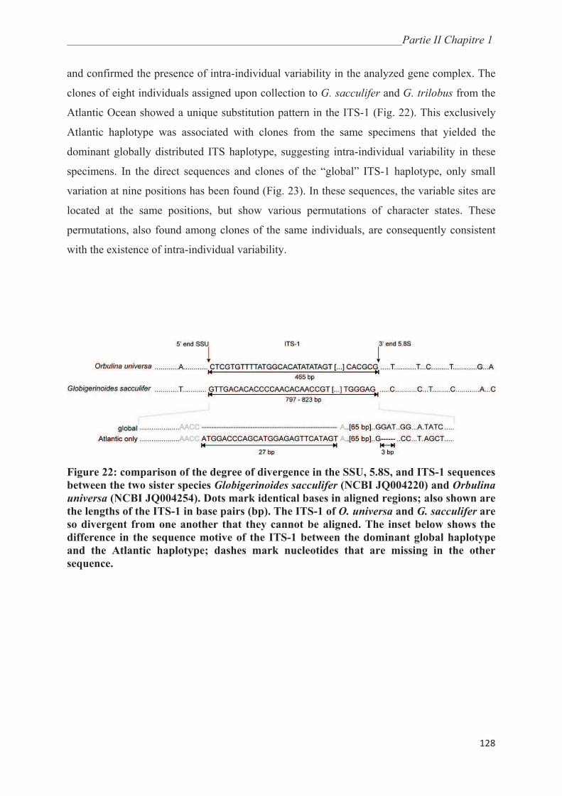
_______________________________________________________________________Partie II Chapitre 1
128
and confirmed the presence of intra-individual variability in the analyzed gene complex. The
clones of eight individuals assigned upon collection to G. sacculifer and G. trilobus from the
Atlantic Ocean showed a unique substitution pattern in the ITS-1 (Fig. 22). This exclusively
Atlantic haplotype was associated with clones from the same specimens that yielded the
dominant globally distributed ITS haplotype, suggesting intra-individual variability in these
specimens. In the direct sequences and clones of the “global” ITS-1 haplotype, only small
variation at nine positions has been found (Fig. 23). In these sequences, the variable sites are
located at the same positions, but show various permutations of character states. These
permutations, also found among clones of the same individuals, are consequently consistent
with the existence of intra-individual variability.
Figure 22: comparison of the degree of divergence in the SSU, 5.8S, and ITS-1 sequences
between the two sister species Globigerinoides sacculifer (NCBI JQ004220) and Orbulina
universa (NCBI JQ004254). Dots mark identical bases in aligned regions; also shown are
the lengths of the ITS-1 in base pairs (bp). The ITS-1 of O. universa and G. sacculifer are
so divergent from one another that they cannot be aligned. The inset below shows the
difference in the sequence motive of the ITS-1 between the dominant global haplotype
and the Atlantic haplotype; dashes mark nucleotides that are missing in the other
sequence.

_______________________________________________________________________Partie II Chapitre 1
129
Figure 23: A, SSU-based phylogenetic tree for all available sequences (Supplementary
Table 1) of the Globigerinoides sacculifer plexus using the three genotypes of Orbulina
universa as outgroup. For details see material and methods. B, Median-joining network
based on a manual alignment of 594 bp in the ITS-1 region of 78 sequences of the G.
sacculifer plexus. Calculation of this haplotype network excludes all parsimony-
uninformative sites. The original output was manually modified for legibility. Lines
represent substitutions between haplotypes; gray lines connect haplotypes that may be
encountered in the same individual; dotted lines, not to scale, indicate more than three
substitutions (number given above the lines). Size of the circles is proportionate to the
number of sequences per haplotype. The largest haplotype difference (34 substitutions)
is a result of two inserts and one deletion, as shown in Figure 22.
None of the observed small differences in the SSU and in the ITS-1 are linked with
morphological differentiation between individuals that were attributed to one of the
Globigerinoides trilobus, G. quadrilobatus, G. immaturus or G. sacculifer s.s. morphotypes
(Fig. 24). An ANOSIM nonparametric test (Clarke 1993) indicates that there is no correlation
between genetic distance and morphology (R = -0.010; p(R = 0) = 0.565 [10,000 permutations]).

_______________________________________________________________________Partie II Chapitre 1
130
Figure 24: MUSCLE alignments-based ITS genetic diversity within the Globigerinoides
sacculifer plexus and within the morphospecies Truncorotalia truncatulinoides and
Globoconella inflata (data from de Vargas et al. 2001 and Morard et al. 2011,
respectively). Box plots give the mean (black circles), 1st through3
rd quartiles (open
rectangles), and 95% confidence interval (lines) patristic distance values expressed as
percent of nucleotide changes within the entire plexus (G. sacculifer s.l.) and within each
of the four morphotypes of the plexus. For T. truncatulinoides and G. inflata, the
patristic genetic distances within genotypes (Types I to IV of T. truncatulinoides, Types I
and II of G. inflata) are also given. Note the changes in the left-hand scale of patristic
distances.
_______________________________________________________________________Partie II Chapitre 1
131
4. Discussion
4.1. Genetic Diversity in Globigerinoides sacculifer
The results of our survey of the G. sacculifer plexus are in stark contrast with the
expectation based on other species of planktonic foraminifera. All extensively genetically
studied morphospecies of modern planktonic foraminifera have so far revealed the presence
of more than one distinct genetic type (see review in Darling and Wade 2008). The absence of
genetic variability in the SSU rDNA region within the global population of the plexus
contrasts with the large differences among genetic types in all other intensively studied
spinose planktonic foraminiferal species (Göker et al. 2010). However, this alone cannot be
taken as unambiguous evidence for the absence of genetic types. In the non-spinose
planktonic foraminiferal species Truncorotalia truncatulinoides (de Vargas et al. 2001) and
Globoconella inflata (Morard et al. 2011), inter-genotype variability consistently appears at
the level of the faster-evolving ITS-1 region.
To exclude the possibility that genetic differentiation in the Globigerinoides sacculifer
plexus is also first manifested in this region, we have supplemented the SSU rDNA survey
with a large data set of partial and complete ITS-1 sequences. These ITS-1 sequences show a
higher degree of variability than the SSU data, which appears in two different ways. First, one
consistent sequence pattern (haplotype) was found only in the Atlantic, and second, a number
of minor variations (SNPs) were found throughout the world ocean (Fig. 23). This degree of
variation is consistent with a population-level signal, and the number of substitutions
separating individuals is more than 15 times lower than among ITS-1 genotypes of both
Truncorotalia truncatulinoides and Globoconella inflata (Fig. 24 and Table 15), which
constitute the only reference points for this rDNA array. The available ITS-1 data on the G.
sacculifer plexus thus do not indicate the presence of distinct genetic types and the observed
variability is not correlated with morphological taxonomy within the plexus.
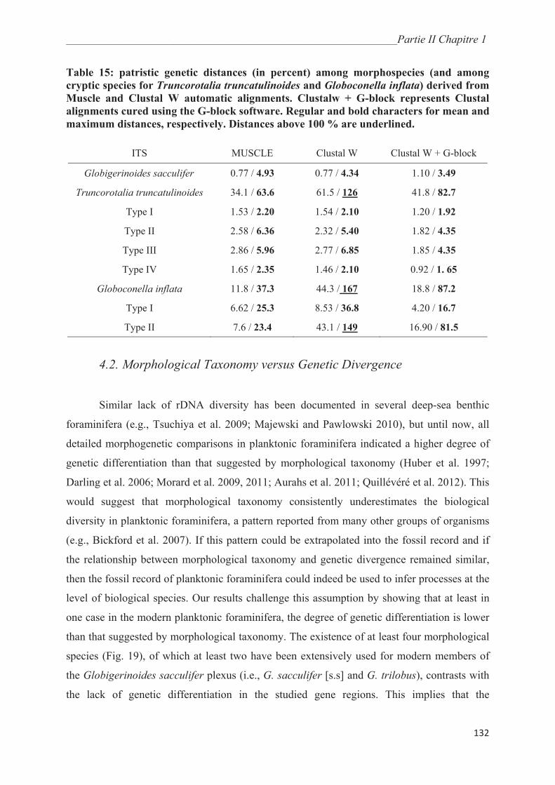
_______________________________________________________________________Partie II Chapitre 1
132
Table 15: patristic genetic distances (in percent) among morphospecies (and among
cryptic species for Truncorotalia truncatulinoides and Globoconella inflata) derived from
Muscle and Clustal W automatic alignments. Clustalw + G-block represents Clustal
alignments cured using the G-block software. Regular and bold characters for mean and
maximum distances, respectively. Distances above 100 % are underlined.
ITS MUSCLE Clustal W Clustal W + G-block
Globigerinoides sacculifer 0.77 / 4.93 0.77 / 4.34 1.10 / 3.49
Truncorotalia truncatulinoides 34.1 / 63.6 61.5 / 126 41.8 / 82.7
Type I 1.53 / 2.20 1.54 / 2.10 1.20 / 1.92
Type II 2.58 / 6.36 2.32 / 5.40 1.82 / 4.35
Type III 2.86 / 5.96 2.77 / 6.85 1.85 / 4.35
Type IV 1.65 / 2.35 1.46 / 2.10 0.92 / 1. 65
Globoconella inflata 11.8 / 37.3 44.3 / 167 18.8 / 87.2
Type I 6.62 / 25.3 8.53 / 36.8 4.20 / 16.7
Type II 7.6 / 23.4 43.1 / 149 16.90 / 81.5
4.2. Morphological Taxonomy versus Genetic Divergence
Similar lack of rDNA diversity has been documented in several deep-sea benthic
foraminifera (e.g., Tsuchiya et al. 2009; Majewski and Pawlowski 2010), but until now, all
detailed morphogenetic comparisons in planktonic foraminifera indicated a higher degree of
genetic differentiation than that suggested by morphological taxonomy (Huber et al. 1997;
Darling et al. 2006; Morard et al. 2009, 2011; Aurahs et al. 2011; Quillévéré et al. 2012). This
would suggest that morphological taxonomy consistently underestimates the biological
diversity in planktonic foraminifera, a pattern reported from many other groups of organisms
(e.g., Bickford et al. 2007). If this pattern could be extrapolated into the fossil record and if
the relationship between morphological taxonomy and genetic divergence remained similar,
then the fossil record of planktonic foraminifera could indeed be used to infer processes at the
level of biological species. Our results challenge this assumption by showing that at least in
one case in the modern planktonic foraminifera, the degree of genetic differentiation is lower
than that suggested by morphological taxonomy. The existence of at least four morphological
species (Fig. 19), of which at least two have been extensively used for modern members of
the Globigerinoides sacculifer plexus (i.e., G. sacculifer [s.s] and G. trilobus), contrasts with
the lack of genetic differentiation in the studied gene regions. This implies that the

_______________________________________________________________________Partie II Chapitre 1
133
morphological variability within the plexus has been, so far uniquely among planktonic
foraminifera, taxonomically over-interpreted.
To underline the anomalous lack of genetic differentiation within the Globigerinoides
sacculifer plexus, we have compiled data on the number of genetic types, number of
synonyms, ages, and abundances of seven morphospecies of modern spinose planktonic
foraminifera for which extensive genetic data are available (Fig. 25). Whereas there does not
appear to be any relationship between the number of genetic types and abundance (expressed
as mean number of CHRONOS reports of the species per million years), we observe positive
correlation between the number of genetic types and age of the morphospecies and the
number of synonyms that exist for the morphospecies. In both cases, G. sacculifer deviates
from the general relationship. Interestingly, next to G. sacculifer, the largest deviation from
the relationship is shown by Orbulina universa, the sister species to G. sacculifer. When both
species are removed, the coefficients of determination increase from 0.09 to 0.73 for species
age and from 0.27 to 0.87 for the number of synonyms (Fig. 25). We note that the estimate of
the number of synonyms for each of the analyzed species is fraught with a considerable level
of subjectivity. For example, when only synonyms that appear in the CHRONOS database are
used, the deviation of O. universa and G. sacculifer from the rest of the test group remains,
but the correlation within the rest of the test group is much weaker.
Figure 25: relationships between the number of reported SSU rDNA genotypes in the
seven extensively studied spinose planktonic foraminiferal morphospecies and the
average number of the morphospecies reports per million years from the CHRONOS
database (A), the age of the morphospecies (after Kucera and Schönfeld 2007; Aurahs et
al. 2011) (B), and the number of junior synonyms for the morphospecies collated from
the literature (open symbols: Saito et al. 1981; Kennett and Srinivasan 1983) and from
the CHRONOS database (black symbols) (C). Dotted lines in B and C indicate linear
regressions for all species (in C for literature synonyms); solid lines indicate linear
regressions without G. sacculifer and O. universa (see text). Coefficients of determination
for regression without those two species are significant at the 5% level (t-test for r = 0),
but we note that the sample size in this case is too small for a robust statistical
assessment.
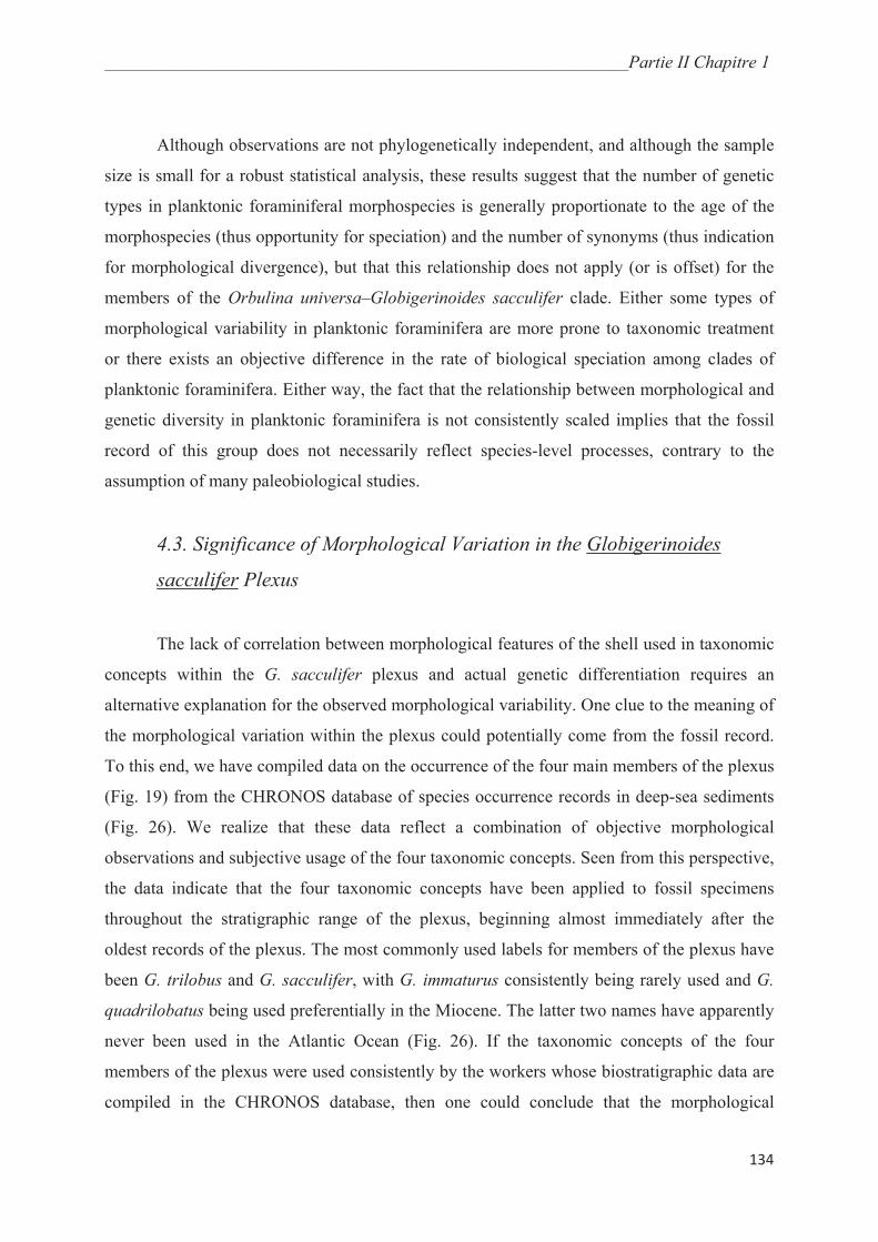
_______________________________________________________________________Partie II Chapitre 1
134
Although observations are not phylogenetically independent, and although the sample
size is small for a robust statistical analysis, these results suggest that the number of genetic
types in planktonic foraminiferal morphospecies is generally proportionate to the age of the
morphospecies (thus opportunity for speciation) and the number of synonyms (thus indication
for morphological divergence), but that this relationship does not apply (or is offset) for the
members of the Orbulina universa–Globigerinoides sacculifer clade. Either some types of
morphological variability in planktonic foraminifera are more prone to taxonomic treatment
or there exists an objective difference in the rate of biological speciation among clades of
planktonic foraminifera. Either way, the fact that the relationship between morphological and
genetic diversity in planktonic foraminifera is not consistently scaled implies that the fossil
record of this group does not necessarily reflect species-level processes, contrary to the
assumption of many paleobiological studies.
4.3. Significance of Morphological Variation in the Globigerinoides
sacculifer Plexus
The lack of correlation between morphological features of the shell used in taxonomic
concepts within the G. sacculifer plexus and actual genetic differentiation requires an
alternative explanation for the observed morphological variability. One clue to the meaning of
the morphological variation within the plexus could potentially come from the fossil record.
To this end, we have compiled data on the occurrence of the four main members of the plexus
(Fig. 19) from the CHRONOS database of species occurrence records in deep-sea sediments
(Fig. 26). We realize that these data reflect a combination of objective morphological
observations and subjective usage of the four taxonomic concepts. Seen from this perspective,
the data indicate that the four taxonomic concepts have been applied to fossil specimens
throughout the stratigraphic range of the plexus, beginning almost immediately after the
oldest records of the plexus. The most commonly used labels for members of the plexus have
been G. trilobus and G. sacculifer, with G. immaturus consistently being rarely used and G.
quadrilobatus being used preferentially in the Miocene. The latter two names have apparently
never been used in the Atlantic Ocean (Fig. 26). If the taxonomic concepts of the four
members of the plexus were used consistently by the workers whose biostratigraphic data are
compiled in the CHRONOS database, then one could conclude that the morphological
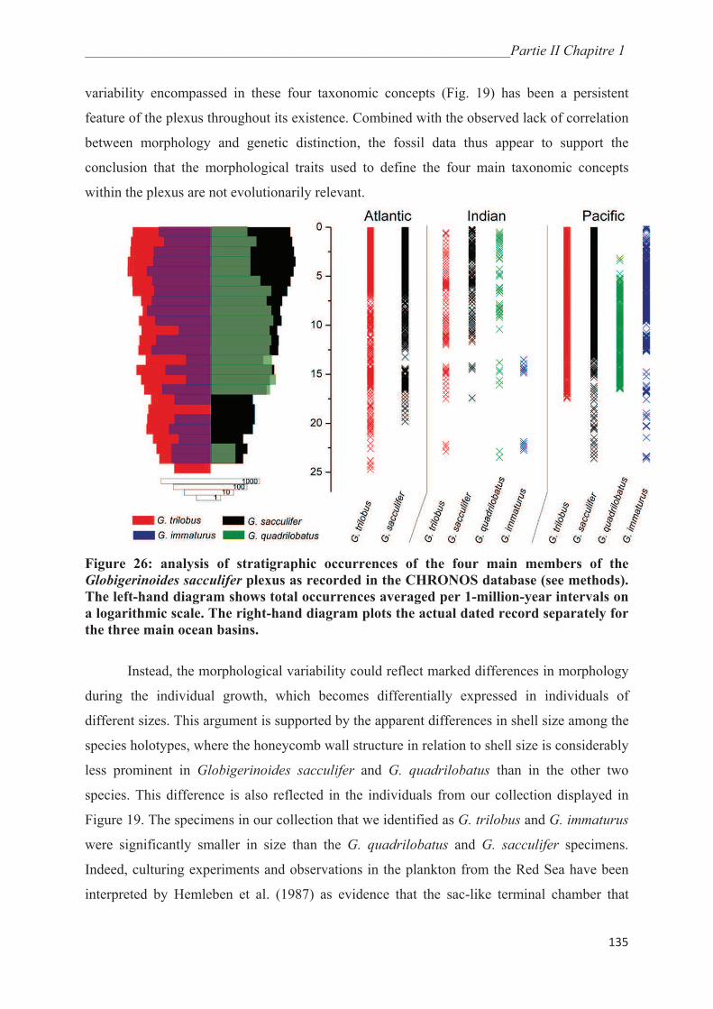
_______________________________________________________________________Partie II Chapitre 1
135
variability encompassed in these four taxonomic concepts (Fig. 19) has been a persistent
feature of the plexus throughout its existence. Combined with the observed lack of correlation
between morphology and genetic distinction, the fossil data thus appear to support the
conclusion that the morphological traits used to define the four main taxonomic concepts
within the plexus are not evolutionarily relevant.
Figure 26: analysis of stratigraphic occurrences of the four main members of the
Globigerinoides sacculifer plexus as recorded in the CHRONOS database (see methods).
The left-hand diagram shows total occurrences averaged per 1-million-year intervals on
a logarithmic scale. The right-hand diagram plots the actual dated record separately for
the three main ocean basins.
Instead, the morphological variability could reflect marked differences in morphology
during the individual growth, which becomes differentially expressed in individuals of
different sizes. This argument is supported by the apparent differences in shell size among the
species holotypes, where the honeycomb wall structure in relation to shell size is considerably
less prominent in Globigerinoides sacculifer and G. quadrilobatus than in the other two
species. This difference is also reflected in the individuals from our collection displayed in
Figure 19. The specimens in our collection that we identified as G. trilobus and G. immaturus
were significantly smaller in size than the G. quadrilobatus and G. sacculifer specimens.
Indeed, culturing experiments and observations in the plankton from the Red Sea have been
interpreted by Hemleben et al. (1987) as evidence that the sac-like terminal chamber that

_______________________________________________________________________Partie II Chapitre 1
136
characterizes the morphotype G. sacculifer s.s. is an ontogenetic feature, not developed on all
individuals that reach reproductive maturity.
Alternatively, the morphological variability within the plexus could represent an
ecophenotypic signal, with different morphologies being expressed under different
environmental conditions. The ecophenotypic plasticity is a typical feature of species of
planktonic foraminifera (e.g., Kennett 1976). For the Globigerinoides sacculifer plexus, Hecht
(1974) studied the distribution of specimens with the sac-like final chamber as well as the
morphology of specimens without the sac-like chamber. He concluded that the abundance of
the sac-like chambers within the plexus increased toward the tropics. This observation is
clearly supported by an analysis of the MARGO North Atlantic data set of coretop
abundances (Fig. 27). Specimens with and without the final sac-like chamber occur within the
same range of temperatures, but the abundance of the G. sacculifer s.s. morphotype increases
with temperature. It is therefore likely that the manifestation of some or all of the
morphological types within the plexus reflects a combination of the existence of different
ontogenetic growth stages, which are differentially reached under different environmental
conditions. As a consequence, our results imply that all modern representatives of the plexus
should be treated as members of a single biological species. Of the four main members of the
plexus, G. sacculifer is the only one whose original description (Brady 1877) refers to it as
occurring in the modern plankton; all other names referring exclusively to fossil material. By
the principle of priority, the name G. quadrilobatus (d’Orbigny 1846) should be considered
the senior synonym for the plexus. However, because we cannot entirely exclude the
possibility that the fossil representatives of the plexus with different morphologies could
represent different species, we propose that the name G. sacculifer be used for all modern
specimens of the plexus. The use of “with sac” or “without sac” (i.e., presence or absence of a
sac-like final chamber) should be used solely as the description of morphotypes within this
species.
_______________________________________________________________________Partie II Chapitre 1
137
Figure 27: left, abundance of Globigerinoides sacculifer with and without the sac-like
terminal chamber in surface sediments of the North Atlantic plotted against caloric
summer SST at 10 m depth (abundance and SST data from Kucera et al. 2005). Right,
proportion of specimens without the sac-like chamber in all samples where the
abundance of both forms together was higher than 5% in the assemblages; the line
shows linear regression; its statistical significance is shown in the figure.
4.4. Global Dispersal and Gene Flow in Globigerinoides sacculifer
The fact that same haplotypes on the SSU and ITS-1 sequences in G. sacculifer are
found globally, throughout the subtropical and tropical habitat of the species, implies either
ongoing and effective gene flows or an extremely reduced substitution rate (see also Darling
et al. 1999). The latter hypothesis is not consistent with the observed existence of insertion
and deletion and polymorphic sites in the ITS-1 region in the species (Fig. 23), which
indicates ongoing intra-population differentiation. In addition, G. sacculifer and Orbulina
universa consistently cluster as sister species in SSU rDNA phylogenies (Darling et al. 1997;
de Vargas and Pawlowski 1998; Aurahs et al. 2009b), but their ITS-1 sequences are so
derived that they cannot be aligned (Fig. 23). As a consequence, we conclude that the lack of
geographic differentiation in G. sacculifer probably does not result from a slowdown in
evolutionary rate. Instead, the data appear more consistent with the existence of an ongoing
(or very recent) effective gene flow among the partly disjunct warm-water populations of the
species between the Indo-Pacific and the Atlantic. Because planktonic foraminifera are
passively dispersed by surface currents, this conjecture implies that the transport of specimens
or propagules of this species by the Agulhas Current and Agulhas Rings from the Indian
Ocean into the South Atlantic is effective enough to saturate the Atlantic population with
specimens carrying Indo-Pacific haplotypes.
Indeed, Peeters et al. (2004) report large standing stocks of Globigerinoides sacculifer
from plankton nets samples retrieved in isolated Agulhas Rings in the Southern Atlantic. The
passive transport of this species into the Atlantic is clearly visible in the pattern of its
_______________________________________________________________________Partie II Chapitre 1
138
abundance in surface sediment samples (Fig. 28). Considering the pattern of surface current
flow between the two oceans (Beal et al. 2011), the advection of G. sacculifer between the
Indo-Pacific and the Atlantic is at present mainly unidirectional. In fact, the transport is likely
to have remained unidirectional since the closure of the Panama Isthmus in the Pliocene
(Groeneveld et al. 2006).
The unidirectionality of the gene flow in Globigerinoides sacculifer from the Indo-
Pacific into the Atlantic is consistent with the occurrence of an exclusively Atlantic ITS-1
haplotype (Fig. 23). We hypothesize that this haplotype originated in allopatry, during an
intermittent isolation of the Atlantic Ocean, but its evolution was not associated with the
development of intrinsic reproductive isolation mechanisms, such that inbreeding was not
prevented upon secondary contact with the Indo-Pacific population. This is evidenced by the
fact that the Atlantic haplotype occurs together with the dominant global haplotype in the
same specimens. Considering that it is only found in the faster-evolving ITS-1 and does not
correspond to a differentiation signal in the SSU, and that there is no evidence for genetic
recombination between the haplotypes, we conclude that its occurrence reflects a recent
isolation event. The most recent opportunity for isolation between the Indo-Pacific and the
Atlantic (sub)tropical water masses occurred during the last glacial maximum, when the
circum-Antarctic currents were displaced toward the north and constricted the Agulhas
exchange (Flores et al. 1999; Peeters et al. 2004; Bard and Rickaby 2009; Beal et al. 2011).
The chance for westward advection of individuals of G. sacculifer around the Cape was thus
considerably reduced, as the environment that had to be crossed to reach the Atlantic became
too cold (Fig. 28), close to the temperature tolerance of the taxon (14-32 °C [Bijma et al.
1990]). The resulting restriction of the passive transport of G. sacculifer around the Cape is
reflected in the abundance of this species in deep-sea sediments from the region that have
been dated to the last glacial maximum (Fig. 28).
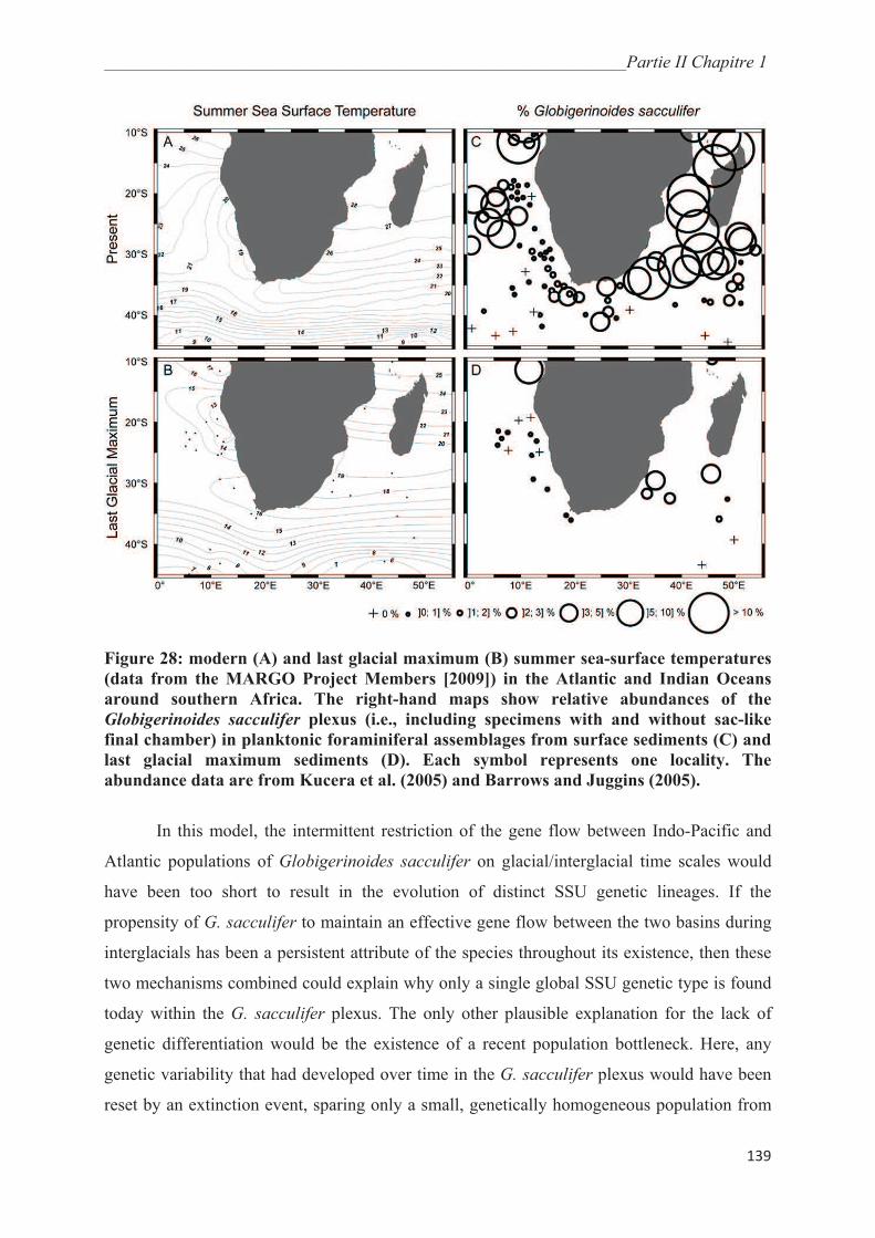
_______________________________________________________________________Partie II Chapitre 1
139
Figure 28: modern (A) and last glacial maximum (B) summer sea-surface temperatures
(data from the MARGO Project Members [2009]) in the Atlantic and Indian Oceans
around southern Africa. The right-hand maps show relative abundances of the
Globigerinoides sacculifer plexus (i.e., including specimens with and without sac-like
final chamber) in planktonic foraminiferal assemblages from surface sediments (C) and
last glacial maximum sediments (D). Each symbol represents one locality. The
abundance data are from Kucera et al. (2005) and Barrows and Juggins (2005).
In this model, the intermittent restriction of the gene flow between Indo-Pacific and
Atlantic populations of Globigerinoides sacculifer on glacial/interglacial time scales would
have been too short to result in the evolution of distinct SSU genetic lineages. If the
propensity of G. sacculifer to maintain an effective gene flow between the two basins during
interglacials has been a persistent attribute of the species throughout its existence, then these
two mechanisms combined could explain why only a single global SSU genetic type is found
today within the G. sacculifer plexus. The only other plausible explanation for the lack of
genetic differentiation would be the existence of a recent population bottleneck. Here, any
genetic variability that had developed over time in the G. sacculifer plexus would have been
reset by an extinction event, sparing only a small, genetically homogeneous population from

_______________________________________________________________________Partie II Chapitre 1
140
which all the modern representatives would have descended. Low levels of genetic diversity
have been shown in planktonic foraminifera thought to have undergone such recent
bottlenecks (e.g., Aurahs et al. 2009a). However, the fossil distribution of the G. sacculifer
plexus does not indicate any evidence for a population bottleneck (Figs. 26, 28). To our
knowledge, in the literature, such an event has never been reported for G. sacculifer at any
time throughout the existence of the species.
_______________________________________________________________________Partie II Chapitre 1
141
5. Conclusions
Our survey of the genetic variability in the modern representatives of the
Globigerinoides sacculifer plexus reveals the existence of a single genetic type. The lack of
cryptic genetic diversity is in stark contrast to the morphological variability and the usage of
multiple taxonomic concepts for members of this plexus. Our results imply that at least in the
modern plankton, the morphospecies G. sacculifer, G. immaturus, G. trilobus, and G.
quadrilobatus all correspond to a single biological species with a cosmopolitan distribution.
In paleoceanographic reconstructions based on morphological and/or chemical signals in the
fossil shells of planktonic foraminifera, the assumption is indirectly made that each
morphospecies corresponds to a biological species adapted to a unique habitat and possessing
unique biomineralization physiology. Over the last decade, this assumption has been called
into question by extensive genetic surveys, which revealed the existence of multiple distinct
and differentially adapted genetic types within individual morphospecies (de Vargas et al.
1999, 2002; Darling and Wade 2008; Morard et al. 2009; Quillévéré et al. 2012). In the case
of G. sacculifer, the assumption of the congruence between morphological and biological
species is violated in the opposite direction: multiple morphotypes correspond to a single
species. This observation is significant because it shows not only that the morphological
taxonomy does not reflect genetic differentiation, but also that the scaling between the two
may be inconsistent.
The lack of geographic structuring among the surveyed specimens is interpreted as
evidence for an effective gene flow from the Indo-Pacific into the Atlantic tropical and
subtropical habitats of the species. The existence of an exclusively Atlantic ITS-1 haplotype
indicates that this gene flow can be intermittently reduced, most likely during glacial
intervals, but the latest disruption apparently has not been sufficient to result in speciation. If
the propensity for “genetic homogenization” following short periods of isolation was a
persistent feature in the evolutionary history of the species, then the fossil record of the G.
sacculifer plexus could be interpreted as the occurrence of a long-ranging single, ecologically
successful, morphologically variable lineage.
_______________________________________________________________________Partie II Chapitre 1
142
Acknowledgments
We thank L. Konecny, M. Bayer, W. Rönnfeld, N. Buchet, Y. Gally, and L. Licari for
technical assistance and G. W. Grimm for comments on the manuscript. Y. Ujiié is also
warmly thanked. We acknowledge the assistance of the Master and the crew of the cruises
during which the presented material has been collected: Pos321 and 334, M69, 72 and 74,
MSM 8 and 15, AMT-8, Revelle, OISO, C-MarZ, Kt-02 and Kt-06, Melville, Gyrafor A and
B. Special thanks are given to the Institut Polaire Français Paul Emile Victor (IPEV). This
work was supported by grants from the IFR41 of Université Lyon1 (F.Q.), from the Institut
National des Sciences de l’Univers (INSU) INTERRVIE program (F.Q.), from the Agence
Nationale de la Recherche (ANR-06-JCJC-0142-01 PALEO-CTD, T.d.G.T.; ANR 09-BLAN-
0348 POSEIDON, C.d.V. and R.M.). A.W., R.A., and M.K. were financed by the Deutsche
Forschungsgemeinschaft (DFG projects KU 2259/2-2 and KU 2259/19-1).

___________________________________________________________Partie II Chapitre 1
143
References
Akaike, H., 1974. A new look at the statistical model identification. Institute of Electrical and
Electronics Engineers Transactions on Automatic Control, 19: 716-723.
Aurahs, R., Göker, M., Grimm, G., Hemleben, V., Hemleben, C., Schiebel, R. and Kucera,
M., 2009. Using the multiple analysis approach to reconstruct phylogenetic
relationships among planktonic foraminifera from highly divergent and length-
polymorphic SSU rDNA sequences. Bioinformatics and Biology Insights, 3: 155-177.
Aurahs, R., Grimm, G., Hemleben, V., Hemleben, C. and Kucera, M., 2009. Geographical
distribution of cryptic genetic types in the planktonic foraminifer Globigerinoides
ruber. Molecular Ecology, 18: 1692-1706.
Aurahs, R., Treis, Y., Darling, K. and Kucera, M., 2011. A revised taxonomic and
phylogenetic concept for the planktonic foraminifer species Globigerinoides ruber
based on molecular and morphometric evidence. Marine Micropaleontology, 79: 1-14.
Aze, T., Ezard, T., Purvis, T., Coxall, H., Stewart, D., Wade, B. and Pearson, P., 2011. A
phylogeny of Cenozoic macroperforate planktonic foraminifera from fossil data.
Biological Reviews 86: 900-927.
Bandelt, H.J., Forster, P. and Röhl, A., 1999. Median Joining networks for inferring
intraspecific phylogenies. Molecular Biology and Evolution, 16: 37–48
Banner, F.T. and Blow, W.H., 1960. Some primary types of species belonging to the
superfamily Globigerinaceae. Contributions from the Cushman Foundation for
Foraminiferal Research, 11: 1–45.
Bard, E. and Rickaby, R.E.M., 2009. Migration of the subtropical front as a modulator of
glacial climate. Nature, 560: 380–384.
Bé, A.W., 1980. Gametogenetic calcification in a spinose planktonic foraminifer,
Globigerinoides sacculifer (Brady). Marine Micropaleontology, 5: 283–310.
Bé, A.W., Anderson, O.R., Faber, W.W. and Caron, D.A., 1983. Sequence of morphological
and cytoplasmic changes during gametogenesis in the planktonic foraminifer
Globigerinoides sacculifer (Brady). Micropaleontology, 29: 319–325.
Beal, L.M., de Ruijter, W.P., Biastoch, A., Zahn, R. and SCOR/WCRP/IAPSO Working
Group 136, 2011. On the role of the Agulhas system in ocean circulation and climate.
Nature, 472: 429–436.
Berggren, W.A., Kent, D.V., Swisher, C.C. and Aubry, M-P., 1995. A revised Cenozoic
geochronology and chronostratigraphy. Geochronology, time scales and global
stratigraphic correlation, SEPM (Society for Sedimentary Geology), Tulsa (Oklahoma).
Bickford, D., Lohman, D.J., Sodhi, N.S., Ng, P.K.L., Meier, R., Winker, K., Ingram, K.K. and
Das, I., 2007. Cryptic species as a window on diversity and conservation. Trends in
Ecology and Evolution, 22:148–155.
Bijma, J., Erez, J. and Hemleben, C., 1990. Lunar and semi-lunar reproductive cycles in some
spinose planktonic foraminifers. Journal of Foraminiferal Research, 20:117–127.

___________________________________________________________Partie II Chapitre 1
144
Bijma, J., Hemleben, C., Oberhänsli, H. and Spindler, M., 1992. The effects of increased
water fertility on tropical spinose planktonic foraminifers in laboratory cultures. Journal
of Foraminiferal Research, 22:242–256.
Brady, H.B., 1877. Supplementary note on the foraminifera of the chalk (?) of the New
Britain group. Geological Magazine London, 4: 534–536.
Budillon, F., Lirer, F., Iorio, M., Macri, P., Sagnotti, L., Vallefuoco, M., Ferraro, L.,
Garziglia, S., Innangi, S., Sahabi, M. and Tonielli, R., 2009. Integrated stratigraphic
reconstruction for the last 80 kyr in deep sector of the Sardinia Channel (Western
Mediterranean). Deep Sea Research Part II, Topical Studies in Oceanography, 56: 725–
737.
Clarke, K.R., 1993. Non-parametric multivariate analysis of changes in community structure.
Australian Journal of Ecology, 18:117–143.
Darling, K.F., Kroon, D., Wade, C.M. and Leigh Brown, A.J., 1996. Molecular phylogeny of
the planktic foraminifera. Journal of Foraminiferal Research, 26: 324-330.
Darling, K.F., Wade, C.M., Kroon, D. and Brown, A.J., 1997. Planktic foraminiferal
molecular evolution and their polyphyletic origins from benthic taxa. Marine
Micropaleontology, 30: 251–266.
Darling, K.F., Wade, C.M., Kroon, D., Brown, A.J.L. and Bijma, J., 1999. The diversity and
distribution of modern planktic foraminiferal small subunit ribosomal RNA genotypes
and their potential as tracers of present and past circulation. Paleoceanography, 14: 3-
12.
Darling, K.F., Kucera, M., Kroon, D. and Wade, C.M., 2006. A resolution for the coiling
direction paradox in Neogloboquadrina pachyderma. Paleoceanography, 21: 1-14.
Darling, K.F. and Wade, C.M., 2008. The genetic diversity of planktic foraminifera and the
global distribution of ribosomal RNA genotypes. Marine Micropaleontology, 67: 216-
238.
d’Orbigny, A., 1846. Foraminifères fossiles du bassin tertiaire de Vienne (Autriche). Gide et
Comp, Paris.
de Vargas, C., Zaninetti, L., Hilbrecht, H. and Pawlowski, J., 1997. Phylogeny and rates of
molecular evolution of planktonic foraminifera: SSU rDNA sequences compared to the
fossil record. Journal of Molecular Evolution, 45: 285-294.
de Vargas, C., and Pawlowski, J., 1998. Molecular versus taxonomic rates of evolution in
planktonic foraminifera. Molecular Phylogenetics and Evolution, 9:463–469.
de Vargas, C., Norris, R.D., Zaninetti, L., Gibb, S.W. and Pawlowski, J., 1999. Molecular
evidence of cryptic speciation in planktonic foraminifers and their relation to oceanic
provinces. Proceedings of the National Academy of Sciences of the United States of
America, 96: 2864-2868.
de Vargas, C., Renaud, S., Hilbrecht, H. and Pawlowski, J., 2001. Pleistocene adaptive
radiation in Globorotalia truncatulinoides: genetic, morphologic, and environmental
evidence. Paleobiology, 27: 104-125.
de Vargas, C., Bonzon, M., Rees, N.W., Pawlowski, J. and Zaninetti, L., 2002. A molecular
approach to biodiversity and biogeography in the planktonic foraminifer Globigerinella
siphonifera (d'Orbigny). Marine Micropaleontology, 45: 101-116.

___________________________________________________________Partie II Chapitre 1
145
Edgar, R.C., 2004. MUSCLE: multiple sequence alignment with high accuracy and high
throughput. Nucleic Acids Research, 32: 1792-1797.
Flores, J.-A., Gersonde, R. and Sierro, F., 1999. Pleistocene fluctuations in the Agulhas
Current Retroflection based on the calcareous plankton record. Marine
Micropaleontology, 37:1–22.
Görker, M., Grimm, G.W., Auch, A.F., Aurahs, R. and Kucera, M., 2010. A clustering
optimization strategy for molecular taxonomy applied to planktonic foraminifera SSU
rDNA. Evolutionary Bioinformatics, 6: 97-112.
Groeneveld, J., Steph, S., Tiedemann, R., Garbe-Schonberg, D., Nurnberg, D. and Sturm, A.,
2006. Pliocene mixed layer oceanography for site 1241 using combined Mg/Ca and 18
O analyses of Globigerinoides sacculifer. Proceedings of the Ocean Drilling
Program, Scientific Results, 202:1–27.
Guindon, S. and Gascuel, O., 2003. A simple, fast, and accurate algorithm to estimate large
phylogenies by maximum likelihood. Systematic Biology, 52:696-704.
Hecht, A.D., 1974. Intraspecific variation in recent populations of Globigerinoides ruber and
Globigerinoides trilobus and their application to paleoenvironmental analysis. Journal
of Paleontology, 48:1217–1234.
Hemleben, C., Spindler, M., Breitinger, I. and Ott., R., 1987. Morphological and
physiological responses of Globigerinoides sacculifer (Brady) under varying laboratory
conditions. Marine Micropaleontology, 12: 305–324.
Hofker, J., 1959. On the splitting of Globigerina. Contributions from the Cushman
Foundation for Foraminiferal Research, 10:1–9.
Huber, B.T., Bijma, J. and Darling, K.F., 1997. Cryptic speciation in the living planktonic
foraminifer Globigerinella siphonifera (d'Orbigny). Paleobiology, 23: 33-62.
Huson, D.H., and Bryant, D., 2006. Application of phylogenetic networks in evolutionary
studies. Molecular Biology and Evolution, 23: 254–267.
Kennett, J.P., 1976. Phenotypic variation in some recent and late Cenozoic planktonic
foraminifera. Foraminifera, Academic Press, New York.
Kennett, J.P. and Srinivasan, M.S., 1983. Neogene Planktonic Foraminifera: a Phylogenetic
Atlas. Hutchinson Ross, Sroudsburg (Pennsylvania).
Kooistra, W., Sarno, D., Balzano, S., Gu, H., Andersen, R.A. and Zingone, A., 2008. Global
diversity and biogeography of Skeletonema species (Bacillariophyta). Protist, 159: 177–
193.
Kucera, M., Weinelt, M., Kiefer, T., Pflaumann, U., Hayes, A., Weinelt, M., Chen, M.,
Mix, A.C., Barrows, T.T., Cortijo, E., Duprat, J., Juggins, S. and Waelbroeck, C., 2005.
Reconstruction of sea-surface temperatures from assemblages of planktonic
foraminifera: multi-technique approach based on geographically constrained calibration
data sets and its application to glacial Atlantic and Pacific Oceans. Quaternary Science
Reviews, 24: 951–998.
Kucera, M., and Schönfeld, J., 2007. The origin of modern oceanic foraminiferal faunas and
Neogene climate change. Micropalaeontological Society Special Publication, 2: 409–
426.
___________________________________________________________Partie II Chapitre 1
146
Larkin, M.A., Blackshields, G., Chenna, N.P., McGettigan, P.A., McWilliam, H., Valentin,
F., Wallace, I.M., Wilm, A., Lopez, R., Thompson, J.D., Gibson, T.J. and Higgins,
D.G., 2007. Clustal W and Clustal X, Version 2.0. Bioinformatics, 23: 2947–2948.
Leroy, L.W., 1939. Some small Foraminifera, Ostracoda and otoliths from the Neogene
(“Miocene”) of the Rokan-Tapanoeli area, central Sumatra. Natuurkundig Tijdschrift
Voor Nederlandsch Indië, 99: 215-296.
Lim, D.I., Kang, S., Yoo, H.S., Jung, H.S., Choi, J.Y., Kim, H.N. and Shin, I.H., 2006. Late
Quaternary sediments on the outer shelf of the Korea Strait and their paleoceanographic
implications. Geo-Marine Letters, 26: 287–296.
Logares, R., Rengefors, K., Kremp, A., Shalchian-Tabrizi, K., Boltovskoy, A., Tengs, T.,
Shurtleff, A. and Klaveness, D., 2007. Phenotypically different microalgal
morphospecies with identical ribosomal DNA: a case of rapid adaptative evolution?
Microbial Ecology, 53: 549-561.
Majewski, W., and Pawlowski, J., 2010. Morphologic and molecular diversity of the
foraminiferal genus Globocassidulina in Admiralty Bay, King George Island. Antarctic
Science, 22:271–281.
MARGO project members, 2009. Constraints on the magnitude and patterns of ocean cooling
at the last glacial maximum. Nature Geoscience, 2: 127-132.
Morard, R., Quillévéré, F., Escarguel, G., Ujiie, Y., de Garidel-Thoron, T. Norris, R.D. and de
Vargas, C., 2009. Morphological recognition of cryptic species in the planktonic
foraminifer Orbulina universa. Marine Micropaleontology, 71: 148-165.
Morard, R., Quillévéré, F., Douady, C.J., de Vargas, C., de Garidel-Thoron, T. and Escarguel,
G., 2011.Worldwide Genotyping in the Planktonic Foraminifer Globoconella inflata:
Implications for Life History and Paleoceanography. Public Library of Science One, 6:
e26665.
Paradis, E., Claude, J. and Strimmer, K., 2004. APE: analyses of phylogenetics and evolution
in R language. Bioinformatics, 20: 289-290.
Pawlowski, J., Bolivar, I., Fahrni, J., de Vargas, C., Gouy, M. and Zaninetti, L., 1997.
Extreme differences in rates of molecular evolution of foraminifera revealed by
comparison of ribosomal DNA sequences and the fossil record. Molecular Biology and
Evolution, 14:498-505.
Pawlowski, J., 2000. Introduction to the molecular systematics of foraminifera.
Micropaleontology, 46: 1-12.
Peeters, F., Acheson, R., Brummer, G.J., de Ruijter, W., Schneider, R., Ganssen, G., Ufkes, E.
and Kroon, D., 2004. Vigorous exchange between the Indian and Atlantic oceans at the
end of the past five glacial periods. Nature 430: 661–665.
Posada, D. and Crandall, K.A., 1998. Modeltest: testing the model of DNA substitution.
Bioinformatics, 14: 817-818.
Quillévéré, F., Morard, R., Escarguel, G., Douady, C.J., Ujiie, Y., de Garidel-Thoron, T. and
de Vargas, C., in press. Global scale same-specimen morpho-genetic analysis of
Truncorotalia truncatulinoides: A perspective on the morphological species concept in
planktonic foraminifera. Palaeogeography, Palaeoclimatology, Palaeoecology.
R Development Core Team, 2004. R: a language and environment for statistical computing.
___________________________________________________________Partie II Chapitre 1
147
Reuss, A.E., 1850. Neue Foraminiferen aus den Schichten des österreichischen
Tertiarbeckens. Denkschriften der Kaiserlichen Akademie der Wissenschaften,
Mathematisch-Naturwissenschaftliche Classe 1: 365–390.
Saez, A.G., Probert, I., Geisen, M., Quinn, P., Young, J.R. and Medlin, L.K., 2003.
Pseudocryptic speciation in coccolithophores. Proceedings of the National Academy of
Sciences of the United States of America, 100: 7163–7168.
Saito, T., Thomson, P.R. and Berger, D., 1981. Systematic index of Recent and Pleistocene
planktonic foraminifera. University of Tokyo Press, Tokyo.
Saitou, N. and Nei, M., 1987. The neighbor-joining method: a new method for reconstructing
phylogenetic trees. Molecular Biology and Evolution, 4: 406-425.
Siani, G., Paterne, M., and Colin, C., 2010. Late glacial to Holocene planktic foraminifera
bioevents and climatic record in the South Adriatic Sea. Journal of Quaternary Science,
25: 808–821.
Siccha, M., Trommer, G., Schulz, H., Hemleben, C. and Kucera, M., 2009. Factors
controlling the distribution of planktonic foraminifera in the Red Sea and implications
for the development of transfer functions. Marine Micropaleontology, 72:146–156.
Spooner, M. I., Barrows, T.T., De Deckker, P. and Paterne, M., 2005. Palaeoceanography of
the Banda Sea, and Late Pleistocene initiation of the northwest monsoon. Global and
Planetary Change, 49: 28–46.
Tolderlund, D.S. and Bé, A.W.H., 1971. Seasonal distribution of planktonic foraminifera in
the western North Atlantic. Micropaleontology, 17: 297–329.
Tsuchiya, M., Grimm, G.W., Heinz, P., Stögerer, K., Ertan, K., Collen, J., Brüchert, V.,
Hemleben, C., Hemleben, V. and Kitazato, H., 2009. Ribosomal DNA shows extremely
low genetic divergence in a worldwide distributed, but disjunct and highly adapted
marine protozoan (Virgulinella fragilis, Foraminiferida). Marine Micropaleontology,
70: 8–19
Ujiie, Y. and Lipps, J.H., 2009. Cryptic diversity in planktic foraminifera in the northwest
Pacific Ocean. Journal of Foraminiferal Research, 39: 145-154.
Ujiié, Y., de Garidel-Thoron, T., Watanabe, S., Wiebe, P. and de Vargas, C., 2010. Coiling
dimorphism within a genetic type of the planktonic foraminifer Globorotalia
truncatulinoides. Marine Micropaleontology, 77: 145-153.
Wade, C., Darling, K., Kroon, D. and Brown, A., 1996. Early evolutionary origin of the
planktonic foraminifera inferred from SSU rDNA sequences comparison. Journal of
Molecular Evolution, 43: 672–677.
Williams, M., Schmidt, D.N., Wilkinson, I.P., Miller, C.G. and Taylor, P.D., 2006. The type
material of the Miocene to Recent species Globigerinoides sacculifer (Brady) revisited.
Journal of Micropaleontology, 25:153–156.
Wilson, B., 2012. Biogeography and ecostratigraphy of Late Quaternary planktonic
foraminiferal taphocoenoses in the Leeward Islands, Lesser Antilles, NE Caribbean Sea.
Marine Micropaleontology, 86:1–10.


_______________________________________________________________________Partie II Chapitre 2
148
Chapitre 2 : un cas particulier, Neogloboquadrina
pachyderma, morpho-espèce présentant une diversité
morphologique d’origine écophénotypique
Ce deuxième chapitre s’intéresse au cas particulier des types génétiques de
Neogloboquadrina pachyderma, au sens de Darling et al. (2006), c’est-à-dire n’incluant que
les morphotypes sénestres, présents dans l’hémisphère sud. Cette morpho-espèce est
fondamentale pour les reconstructions de l’océan austral, une région clef dans la régulation du
climat global. Cette étude confirme que les trois types génétiques (II, III, IV) récoltés au
niveau de l’océan austral présentent des distributions biogéographiques corrélées à la
température mais aussi à la productivité primaire, ce qui ouvrirait la voie à l’amélioration des
reconstructions paléocéanographiques de l’océan austral. Les Types III et IV de N.
pachyderma présentent une forte diversité morphologique mais, contrairement à ce qui a été
montré chez d’autres foraminifères planctoniques, les variations morphologiques ne reflètent
pas la variabilité génétique au sein de cette morpho-espèce. Les Types III et IV de N.
pachyderma, qui correspondent à des espèces distinctes (Partie I, chapitre 1) particulièrement
divergentes (Partie I, chapitre 2), constituent donc le premier cas avéré de véritables espèces
cryptiques chez les foraminifères planctoniques. L’origine des variations morphologiques
(taille, contour, nombre de loges sur le dernier tour, taille de la dernière loge) est, chez ces
types génétiques, d’origine écophénotypique.
Mots-clefs : Neogloboquadrina pachyderma, océan austral, biogéographie, morphométrie,
éco-phénotypes
Fiches-méthodes : I, II, III, IV, V, VI
Ce manuscrit est en cours de préparation
Ont participé à ce chapitre : Aurore ANDRE (récolte, analyses, interprétations, rédaction),
Frédéric QUILLEVERE (interprétations, rédaction), Elisabeth MICHEL (récolte), Christophe
DOUADY (conseils pour les analyses moléculaires)
_______________________________________________________________________Partie II Chapitre 2
149
Cryptic diversity and ecophenotypy in Neogloboquadrina
pachyderma (planktonic foraminifera): molecular, morphological
and environmental evidences from the Austral Ocean
Abstract
The Austral Ocean plays a key role in climate dynamics but because the use of most of
the classical paleothermometers is limited in (sub)polar waters, obtaining robust estimates of
Quaternary sea surface temperatures (SST) in this region remains challenging. In particular,
planktonic foraminiferal assemblages there are not sufficiently diversified for the application
of environmental transfer functions. (Sub)polar planktonic foraminifera are strongly
dominated by the morpho-species Neogloboquadrina pachyderma and the resulting near-
monospecific assemblages contain too little information to assign precise SST estimates.
Recent morpho-genetic studies in several morpho-species of planktonic foraminifera have
however shown that there is morphological and environmental differentiation among genetic
types of these organisms, and that such additional information can be used to increase the
resolving power of the transfer functions. Here, we present single-specimen combined
molecular and morphological analyses performed on living N. pachyderma collected from
plankton nets across a latitudinal environmental transect in the south Indian Ocean. Based on
the development of a new RFLP protocol, we discriminate three genetic types of N.
pachyderma (Types II, III and IV) in our samples. Our data confirm previous investigations
from the South Atlantic. The distribution pattern of these (sub)polar genetic types is primarily
controlled by SST and primary productivity variations observed across the oceanic fronts of
the Austral Ocean. Finally, our data show that contrary to other morpho-species of planktonic
foraminifera, there is no correlation between morphological and molecular differentiation in
austral N. pachyderma. Rather, the important observed shell shape and size variations are
ecophenotypic; they occur within each genetic type along latitudinal gradients. The austral
genetic types of N. pachyderma therefore constitute a first demonstrated case for true cryptic
diversity within modern morpho-species of planktonic foraminifera.
Keywords: Neogloboquadrina pachyderma, Austral Ocean, biogeography, morphometrics,
eco-phenotype
_______________________________________________________________________Partie II Chapitre 2
150
1. Introduction
Fossil shells of planktonic foraminifera preserved in marine sediments constitute a
major proxy for reconstructing Quaternary climate changes (e.g. Pflaumann et al., 1996;
Kucera, 2007). Many of these reconstructions rely on quantitative empirical calibrations
between extant environmental parameters of the surface oceans and the relative abundance of
current morpho-species in surface sediments (CLIMAP, 1981; MARGO, 2009). Assuming
that each of the counted morpho-species of planktonic foraminifera has a specific, stable
through time relationship to water mass properties, these so call environmental transfer
functions require a precise assessment of the ecology of modern species. Because the use of
such species specific paleoproxy also requires an accurate level of taxonomic consistency, the
morphological definition of these species has been set very broadly and morphological
variations below the level of the morpho-species have been mostly regarded as ecophenotypy
(e.g. Ericson, 1959; Banner and Blow, 1960).
Molecular study techniques applied to planktonic foraminifera have revealed a high
level of genetic diversity within these organisms and challenge the ecological significance of
the broadly defined morpho-species (e.g. Huber et al., 1997; de Vargas et al., 1999; de Vargas
et al., 2001; Darling et al., 2007; Morard et al., 2011; Weiner et al., 2012; Ujiié et al., 2012).
Phylogenetic analyses of ribosomal DNA of material sampled from plankton tows in the
world oceans allowed to show that most of the morpho-species are made of several genetic
types that are at least partially separated environmentally and geographically (see Darling and
Wade, 2008 and André et al., in prep for reviews). Such environmental separation, associated
with the large divergence values occurring among genetic types and the high degree of
genetic similarity occurring within each type, strongly suggests that they correspond to
genuine biological species (André et al., in prep.).
It has been shown in addition that morphological variations within certain morpho-
species, for a long time treated as ecophenotypic variants, represent characters distinguishing
among genetic types adapted to different water mass properties (Huber et al., 1997; de Vargas
et al., 1999; 2001; Darling et al., 2006; Morard et al., 2009; 2011; Aurahs et al., 2011;
Quillévéré et al., 2013). Such morphological characteristics, together with the presence of
additional environmental information resulting from narrower ecological preferences of the
genetic types, are clearly beneficial for paleoceanographers. They allow increasing the
resolving power of the paleoceanographic reconstructions based on foraminiferal counts

_______________________________________________________________________Partie II Chapitre 2
151
(Kucera and Darling, 2002; Morard et al., 2013) and open up the research potential to transfer
the information acquired through genetic analysis to the fossil record.
The Southern Ocean plays a key role in Quaternary climate dynamics. It constitutes
the most important junction of the oceanic circulation, then controlling heat exchanges in the
world ocean, and plays a major role in ocean chemistry (Broecker, 1982; Keir, 1988; Beckey
and Gersonde, 2003). Furthermore, the circum-Antarctic current promoted the formation of
Antarctica ice sheets which triggered global cooling of climates from the Oligocene (Zachos
et al., 2001). Consequently, reconstructing past oceanic conditions in the Austral regions of
the oceans is mandatory for our understanding of Quaternary climates. Unfortunately, at high
latitudes of the south hemisphere, planktonic foraminiferal assemblages are strongly
dominated by the single morpho-species Neogloboquadrina pachyderma, which accounts for
~75% to 100% of the assemblages (MARGO project members, 2009; Fig. 29). Since the
prerequisite for the application of transfer functions is the presence of multiple species in the
analyzed assemblages, surface sediments there contain too little information for their
application. The use of other proxies of sea surface temperature reonstructions is also limited
in (sub)polar waters. For example, 18
O of polar waters, Mg/Ca ratios of planktonic
foraminifera or alkenone saturation ratios of phytoplankton are often conflicting when
estimating high latitude temperatures (Barker et al., 2005). Furthermore, proxies involving
calcite shells analysis may be impacted either by carbonate dissolution or by salinity
variations due to ice formation (Katz et al., 2010) and the high latitude alkenone producers
remain uncertain (de Vernal et al., 2006). Considering the importance of obtaining estimates
of water mass properties in Austral regions, studying morpho-genetic diversity and ecology in
N. pachyderma may offer the opportunity to develop more accurate estimates. Indeed, Morard
et al. (2013) showed that temperatures estimated through transfer functions were significantly
more accurate when the 11 genetic types of 4 low to mid latitude morpho-species were
included in the calibration datasets. Consequently, investigating N. pachyderma genetic
diversity is a condition for applying this approach to Austral Ocean reconstructions.
Darling et al. (2006) evidenced that right and left coiling morphotypes of N.
pachyderma are clearly distinct species that diverged during the Late Miocene. Consequently,
in this paper, we refer to left coiling morphotypes as N. pachyderma and right coiling
morphotypes as Neogloboquadrina incompta (Cifelli, 1961). Neogloboquadrina pachyderma
is a non-spinose macroperforate species (Hemleben et al., 1989; Aze et al., 2011) which is
abundant in sub-polar to polar waters of both hemispheres (Margo project members, 2009)
_______________________________________________________________________Partie II Chapitre 2
152
where it can over-winter in sea-ice (Dieckmann et al., 1991). This morpho-species is highly
diverse morphologically. The number of chambers on the last whorl varies from 4 to 5
(Kennett and Srinivasan, 1983), the aperture ranges from a narrow slit to a high arched
opening (Bandy, 1972; Kennett and Srinivasan, 1983) and the terminal chamber is often of
reduced size (“kummerform” chamber, Olsson, 1973).
Sequencing of a ~1000 base pair (bp) fragment located at the 3’end of the small sub-
unit region of the ribosomal genes (SSU rDNA) showed that N. pachyderma is a cluster of 7
genetic types (Darling et al., 2004; 2007). The Types I and VII are restricted to the polar
waters of the North Atlantic and North Pacific, respectively, whereas the Types V and VI
have been found isolated in the Benguela upwelling system only (Darling et al., 2007). South
Atlantic representatives of N. pachyderma form a cluster of three genetic types, termed Types
II, III and IV (Darling et al., 2004).
This paper focuses on the genetic types of N. pachyderma in the Southern Ocean. As
Darling et al. (2004) suggested that the distribution of these types may be linked to the
position of sub-polar and polar oceanic fronts, investigating morpho-genetic diversity in
austral N. pachyderma paves the way for the development of new paleoceanographic markers
for more precise reconstructions. Consequently, our first aim is to test if the latitudinal
distribution of the genetic types observed in the South Atlantic Ocean (Darling et al., 2004)
may be generalized to the whole Austral Ocean. For this, we describe and compare latitudinal
distributions of the Types II, III and IV along a South Indian Ocean collecting transect that
occurred during the years 2011 and 2012. Using genetic types of N. pachyderma as
paleoceanographic markers would require their morphological identification in the fossil
record. Previous studies (Eynaud et al., 2009; Moller et al., 2013) based on northern
hemisphere N. pachyderma (Type I) suggested high eco-phenotypic variability within N.
pachyderma while, for other morpho-species, genetic types are distinguishable through
morphological features (Huber et al., 1997; de Vargas et al., 1999; 2001; Darling et al., 2006;
Morard et al., 2009; 2011; Aurahs et al., 2011; Quillévéré et al., 2013). Thus, our second aim
is to determine how morphological variations, genetic diversity and environmental conditions
are linked within southern genetic types of N. pachyderma.
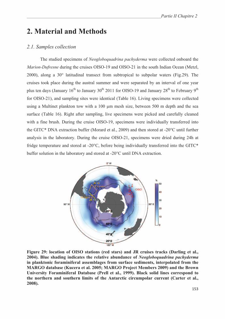
_______________________________________________________________________Partie II Chapitre 2
153
2. Material and Methods
2.1. Samples collection
The studied specimens of Neogloboquadrina pachyderma were collected onboard the
Marion-Dufresne during the cruises OISO-19 and OISO-21 in the south Indian Ocean (Metzl,
2000), along a 30° latitudinal transect from subtropical to subpolar waters (Fig.29). The
cruises took place during the austral summer and were separated by an interval of one year
plus ten days (January 16th
to January 30th
2011 for OISO-19 and January 28th
to February 9th
for OISO-21), and sampling sites were identical (Table 16). Living specimens were collected
using a Multinet plankton tow with a 100 μm mesh size, between 500 m depth and the sea
surface (Table 16). Right after sampling, live specimens were picked and carefully cleaned
with a fine brush. During the cruise OISO-19, specimens were individually transferred into
the GITC* DNA extraction buffer (Morard et al., 2009) and then stored at -20°C until further
analysis in the laboratory. During the cruise OISO-21, specimens were dried during 24h at
fridge temperature and stored at -20°C, before being individually transferred into the GITC*
buffer solution in the laboratory and stored at -20°C until DNA extraction.
Figure 29: location of OISO stations (red stars) and JR cruises tracks (Darling et al.,
2004). Blue shading indicates the relative abundance of Neogloboquadrina pachyderma
in planktonic foraminiferal assemblages from surface sediments, interpolated from the
MARGO database (Kucera et al. 2005; MARGO Project Members 2009) and the Brown
University Foraminiferal Database (Prell et al., 1999). Black solid lines correspond to
the northern and southern limits of the Antarctic circumpolar current (Carter et al.,
2008).
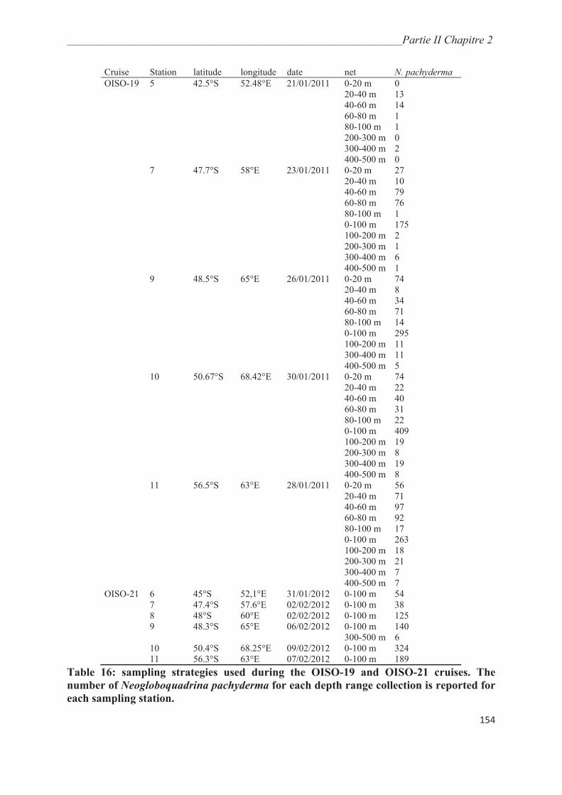
_______________________________________________________________________Partie II Chapitre 2
154
Cruise Station latitude longitude date net N. pachyderma
OISO-19 5 42.5°S 52.48°E 21/01/2011 0-20 m 0
20-40 m 13
40-60 m 14
60-80 m 1
80-100 m 1
200-300 m 0
300-400 m 2
400-500 m 0
7 47.7°S 58°E 23/01/2011 0-20 m 27
20-40 m 10
40-60 m 79
60-80 m 76
80-100 m 1
0-100 m 175
100-200 m 2
200-300 m 1
300-400 m 6
400-500 m 1
9 48.5°S 65°E 26/01/2011 0-20 m 74
20-40 m 8
40-60 m 34
60-80 m 71
80-100 m 14
0-100 m 295
100-200 m 11
300-400 m 11
400-500 m 5
10 50.67°S 68.42°E 30/01/2011 0-20 m 74
20-40 m 22
40-60 m 40
60-80 m 31
80-100 m 22
0-100 m 409
100-200 m 19
200-300 m 8
300-400 m 19
400-500 m 8
11 56.5°S 63°E 28/01/2011 0-20 m 56
20-40 m 71
40-60 m 97
60-80 m 92
80-100 m 17
0-100 m 263
100-200 m 18
200-300 m 21
300-400 m 7
400-500 m 7
OISO-21 6 45°S 52,1°E 31/01/2012 0-100 m 54
7 47.4°S 57.6°E 02/02/2012 0-100 m 38
8 48°S 60°E 02/02/2012 0-100 m 125
9 48.3°S 65°E 06/02/2012 0-100 m 140
300-500 m 6
10 50.4°S 68.25°E 09/02/2012 0-100 m 324
11 56.3°S 63°E 07/02/2012 0-100 m 189
Table 16: sampling strategies used during the OISO-19 and OISO-21 cruises. The
number of Neogloboquadrina pachyderma for each depth range collection is reported for
each sampling station.
_______________________________________________________________________Partie II Chapitre 2
155
2.2. Hydrographic data
During the cruises OISO-19 and OISO-21, temperature, salinity and chlorophyll-a
fluorescence vertical profiles were obtained at same stations using a Conductivity
Temperature and Depth (CTD) probe. In order to compare our observed distributions of
genetic types of N. pachyderma in the south Indian Ocean to those evidenced at similar
latitudes in the south Atlantic (Darling et al., 2004), we further extracted the temperature data
recorded during these cruises JR19 and JR48 from the World Atlas Database. We built the
temperature and fluorescence profiles for the Atlantic and Indian Oceans using Ocean Data
View 4 (Schlitzer, 2011).
2.3. Sequencing and genotyping
2.2.1. DNA extraction, amplification and sequencing
DNA extractions of 531 specimens from the cruise OISO-19 and of 367 specimens
from the cruise OISO-21 were performed using the GITC* protocol, which allows preserving
the calcareous shells of the planktonic foraminifera for further morpho-genetic comparisons
(Morard et al., 2009; 2011; Quillévéré et al., 2013). Samples were gently shaken and heated at
72°C for one hour; afterward they underwent propanol-ethanol purification. DNA was stored
in 40μl of pure water and stored at -20°C.
We designed new N. pachyderma-specific primers termed NP1fb (5’-
CCGGACACACTGAGGATTGACAGGCAATATC-3’) and NP5r (5’-
CTGTTGGGCTCTGAAAGCAACGAACGTG-3’), which, after a standard PCR protocol
(Initial denaturation: 95°C/10 min; 94°C/30s-54°C/30s-72°C/30s repeated 44 times; Final
extension: 72°C:10min), allow PCR-amplification of the DNA extraction products using a
Thermus acquaticus YT-1 polymerase with 5’ flap endonuclease activity (New England
Biolabs). We amplified a 300 to 350 bp fragment localized at the 3’ end of the SSU
corresponding to the foraminiferal specific variable regions F1 and F2 (Fig. 30) as evidenced
by Darling et al. (1997). This fragment is short but sufficient for distinguishing between the
different genetic types of N. pachyderma. PCR products were sequenced directly using the
primers used for PCR amplification on an ABI prism 3730XL sequencer (Applied
Biosystems) from Biofidal (Vaulx-en-Velin, France) service provider.

_______________________________________________________________________Partie II Chapitre 2
156
2.2.2. Restriction Fragment Length Polymorphism (RFLP) analysis
An alternative method, based on two steps, was developed for faster identification of
the genetic types of N. pachyderma (Fig. 30). After amplification by the primers NP1fb/NP5r
and migration of the PCR products on 3% agarose gel and ethidium bromide coloration, we
found that the Type IV of N. pachyderma matches 300 bp fragments while the Types II and
III match 350 bp fragments. In this first step, specimens of the Type IV were thus directly
characterized. The second step, allowing discrimination between the Types II and III of N.
pachyderma, was achieved based on a RLFP protocol. PCR products were digested using the
endonuclease Taq 1 (New England Biolabs), which cuts at sequence 5’ TGCA 3’. We mixed
5 μl of each PCR product with a solution containing 3.4 μl of distilled water, 1μl of the buffer
supplied by the manufacturer, 0.1 μl of BSA and 0.5 μl of enzyme and then incubated two
hours at 65°C. After migration on 3 % agarose gel and ethidium bromide coloration, the Type
II displayed a two-band pattern (one of the two bands being characteristically located at ~250
pb) and the Type III displayed a four-band pattern (one of the four bands being
characteristically located at ~180 pb; Fig. 30).
Figure 30: genotyping method for austral genetic types of Neogloboquadrina
pachyderma. The region of rDNA corresponds to the last ~1000 bases of N. pachyderma
SSU, V correspond to eukaryotic variables regions, F are foraminifer specific variable
regions (Darling et al., 1997).

_______________________________________________________________________Partie II Chapitre 2
157
2.4. Morphological analyses
Shells of the genotyped or sequenced specimens were first observed under the
dissecting microscope. The number of chambers on the last whorl and the relative size of the
last chamber were reported. The number of kummerform specimens (i.e., specimens for
which the size of the last chamber is equally or less developed than the penultimate chamber
[Berger, 1969]), contra the number of normalform specimens was noted as well. A total of 65
shells, selected in order to maximize the morphological variability at each OISO-19 station,
were further SEM pictured.
59 perfectly preserved shells were retained for further morphometric analyses. The
remaining specimens were excluded from our analyses because of aberrant right-coiling
direction or partly broken last chamber in one and five specimens, respectively. Sizes of the
specimens were estimated using two measurements: the maximum diameter (Dmax) and the
distance between the sutures of the first and third chamber on the last whorl (Dc1-c3) (Fig.
31). The Dmax gives the best overall estimation of the foraminifer size but is clearly
influenced by the size of the last chamber. The Dc1-c3 is not impacted by the size of the last
chamber and is homologous between individuals. We tested whether the genetic types display
different sizes by comparing sizes of the Types III and IV across the entire OISO- 19 transect
using R v. 2.14.1 (R development core Team, 2004). In order to minimize environmental
impact, we also ran the comparison tests for the station 11 alone, which is a particularly well-
sampled station. Likewise, we compared the sizes of the Type III across latitude to detect
putative environmental control over the size of the genetic types of N. pachyderma.
Figure 31: distances used for estimation of the shell size of analyzed Neogloboquadrina
pachyderma.
_______________________________________________________________________Partie II Chapitre 2
158
Following Healy-Williams (1984), shape variation among specimens was appraised
using two-dimensional shell outline analyses in umbilical views. The standard taxonomic
edge view was not analyzed because this position was highly instable in the case of N.
pachyderma, preventing any homologous positioning of the specimens. Each specimen was
SEM photomicrographed and the ChainCoder program of SHAPE v. 1.3 (Iwata and Ukai,
2002) was used to extract shell outlines and to record them as a chain code. The size of the
specimens was standardized thanks to the SEM picture scales.
Shell outlines were analyzed using the elliptical Fourier analysis (Kuhl and Giardina,
1982), which has successfully been applied to many studies of planktonic foraminiferal within
morphospecies shape variations (e.g., de Vargas et al., 2001; Quillévéré et al., 2002; 2013;
Renaud and Schmidt, 2003). In such analysis, any outline is described as a sum of
trigonometric functions of decreasing wave-length, the harmonics (Healy-Williams, 1984;
Foote, 1989), which allow constituting a data set of normalized Fourier descriptors suitable
for statistical comparisons (Kuhl and Giardina, 1982). The Chc2Nef program of SHAPE
calculated the elliptical Fourier descriptors using the chain code. We ran the analysis using
two different normalizations: according to the first harmonic and according to the longest
radius after defining a starting point located at the acute margin of the last chamber. Using the
Princomp program of SHAPE, we appraised the extent of shape differentiation among genetic
types of Neogloboquadrina pachyderma by applying a principal component analysis (PCA) to
the Fourier descriptors data set. Such analysis is based on the variance-covariance matrix of
the descriptors and allows reduction of the inter-individual shape variability to a few principal
components (PCs) that best summarize the overall morphological variation within the dataset.
Using PAST v.2.12 (Hammer et al., 2001), we calculated one-way multivariate analyses of
variance (MANOVA) and associated pairwise tests of significance on the PC in order to test
whether the differences observed between the PCA clusters are statistically significant. In
order to test for correlations between size and morphology, we compared the sizes of the N.
pachyderma among the PCA delineated clusters using R v. 2.14.1 (R development core Team,
2004).
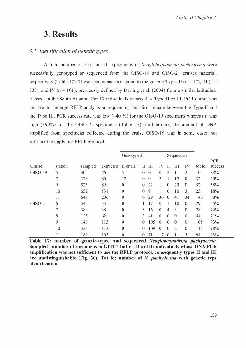
_______________________________________________________________________Partie II Chapitre 2
159
3. Results
3.1. Identification of genetic types
A total number of 257 and 411 specimens of Neogloboquadrina pachyderma were
successfully genotyped or sequenced from the OISO-19 and OISO-21 cruises material,
respectively (Table 17). These specimens correspond to the genetic Types II (n = 17), III (n =
533), and IV (n = 101), previously defined by Darling et al. (2004) from a similar latitudinal
transect in the South Atlantic. For 17 individuals recorded as Type II or III, PCR output was
too low to undergo RFLP analysis or sequencing and discriminate between the Type II and
the Type III. PCR success rate was low (~40 %) for the OISO-19 specimens whereas it was
high (~90%) for the OISO-21 specimens (Table 17). Furthermore, the amount of DNA
amplified from specimens collected during the cruise OISO-19 was in some cases not
sufficient to apply our RFLP protocol.
Genotyped Sequenced
Cruise station sampled extracted II or III II III IV II III IV tot id
PCR
success
OISO-19 5 30 26 5 0 0 0 2 1 2 10 38%
7 378 80 12 0 0 2 1 17 0 32 40%
9 523 89 0 0 22 1 0 29 0 52 58%
10 652 131 0 0 9 1 0 10 3 23 18%
11 649 206 0 0 29 36 0 41 34 140 68%
OISO-21 6 54 53 0 1 17 0 1 10 0 29 55%
7 38 38 0 5 16 0 4 3 0 28 74%
8 125 62 0 3 41 0 0 0 0 44 71%
9 146 113 0 0 105 0 0 0 0 105 93%
10 324 113 0 0 109 0 0 2 0 111 98%
11 189 103 0 0 71 17 0 1 5 94 93%
Table 17: number of genetic-typed and sequenced Neogloboquadrina pachyderma.
Sampled= number of specimens in GITC* buffer. II or III: individuals whose DNA PCR
amplification was not sufficient to use the RFLP protocol, consequently types II and III
are undistinguishable (Fig. 30). Tot id: number of N. pachyderma with genetic type
identification.

_______________________________________________________________________Partie II Chapitre 2
160
3.2. Hydrography and geographic distribution of genetic types
Since both OISO-19 and OISO-21 collecting transects and stations were identical and
occurred at the same period of the year, our dataset allowed us to compare conditions of the
surface Ocean and related distributions of genetic types of N. pachyderma between the years
2011 and 2012. The Sub-Tropical (STF), Sub-Antarctic (SAF) and Polar (PF) Fronts (Ikeda et
al., 1989) were localized along the OISO-19 and OISO-21 transects based on temperature (0-
1000m) vertical profiles (Fig. 32). In the austral summer of 2011 and 2012, temperature
conditions were almost similar with water masses well distributed according to latitude. As
expected, polar waters south of the PF do not show any thermal stratification. Temperature
vertical gradients, however, are visible between surface and deeper waters north of the PF but
at the scale of the photic zone (upper 100m), this thermal stratification remains very weak
throughout the latitudinal transect. We note that at similar period of the year, upper Ocean
temperatures north of the STF and south of the SAF were significantly warmer in 2012 than
in 2011 (Fig. 33). Positive thermal anomalies recorded in 2012 may have impacted surface
water primary productivity, which appears significantly lower in 2012 (Fig. 32). Indeed,
based on chlorophyll-a fluorescence vertical profiles recorded in 2012, we find that north of
the SAF, the transition between oligotrophic and mesotrophic surface waters is particularly
sharp, while it is far patchier in 2011, as a result of probable plankton blooms (diatoms were
extremely abundant at sampling stations).
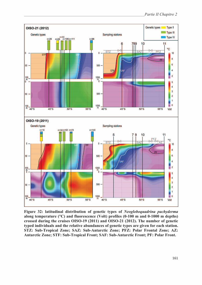
_______________________________________________________________________Partie II Chapitre 2
161
Figure 32: latitudinal distribution of genetic types of Neogloboquadrina pachyderma
along temperature (°C) and fluorescence (Volt) profiles (0-100 m and 0-1000 m depths)
crossed during the cruises OISO-19 (2011) and OISO-21 (2012). The number of genetic
typed individuals and the relative abundances of genetic types are given for each station.
STZ: Sub-Tropical Zone; SAZ: Sub-Antarctic Zone; PFZ: Polar Frontal Zone; AZ:
Antarctic Zone; STF: Sub-Tropical Front; SAF: Sub-Antarctic Front; PF: Polar Front.
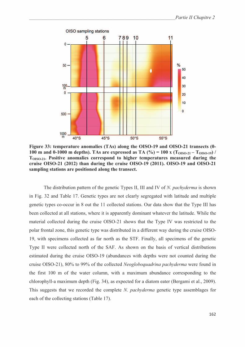
_______________________________________________________________________Partie II Chapitre 2
162
Figure 33: temperature anomalies (TAs) along the OISO-19 and OISO-21 transects (0-
100 m and 0-1000 m depths). TAs are expressed as TA (%) = 100 x (TOISO-21 – TOISO-19) /
TOISO-21. Positive anomalies correspond to higher temperatures measured during the
cruise OISO-21 (2012) than during the cruise OISO-19 (2011). OISO-19 and OISO-21
sampling stations are positioned along the transect.
The distribution pattern of the genetic Types II, III and IV of N. pachyderma is shown
in Fig. 32 and Table 17. Genetic types are not clearly segregated with latitude and multiple
genetic types co-occur in 8 out the 11 collected stations. Our data show that the Type III has
been collected at all stations, where it is apparently dominant whatever the latitude. While the
material collected during the cruise OISO-21 shows that the Type IV was restricted to the
polar frontal zone, this genetic type was distributed in a different way during the cruise OISO-
19, with specimens collected as far north as the STF. Finally, all specimens of the genetic
Type II were collected north of the SAF. As shown on the basis of vertical distributions
estimated during the cruise OISO-19 (abundances with depths were not counted during the
cruise OISO-21), 80% to 99% of the collected Neogloboquadrina pachyderma were found in
the first 100 m of the water column, with a maximum abundance corresponding to the
chlorophyll-a maximum depth (Fig. 34), as expected for a diatom eater (Bergami et al., 2009).
This suggests that we recorded the complete N. pachyderma genetic type assemblages for
each of the collecting stations (Table 17).

_______________________________________________________________________Partie II Chapitre 2
163
Figure 34: depth distribution of Neogloboquadrina pachyderma in the Southern Indian
Ocean (0-500 m). A: black line: distribution of N. pachyderma for all OISO-19 stations;
grey line: cumulative % of N. pachyderma. B: black line: depth distribution of N.
pachyderma for station 7 (cruise OISO-19); grey line: fluorescence profile,
corresponding to Chlorophyll-a, proxy of primary productivity, for the same station.
Unfortunately, due to the low PCR success rate obtained from the OISO-19 material
and the lack of stratified sampling during the cruise OISO-21, depth distributions of the
genetic types remain undetermined except at station 11 from OISO-19 (Fig. 29 and Table 18).
For this station, we notice that the Type III of N. pachyderma is more abundant than the Type
IV in surface waters (0-40 m) whereas in deeper samples (40-80 m), the Type IV significantly
dominates the assemblages (p-value = 0.0018).
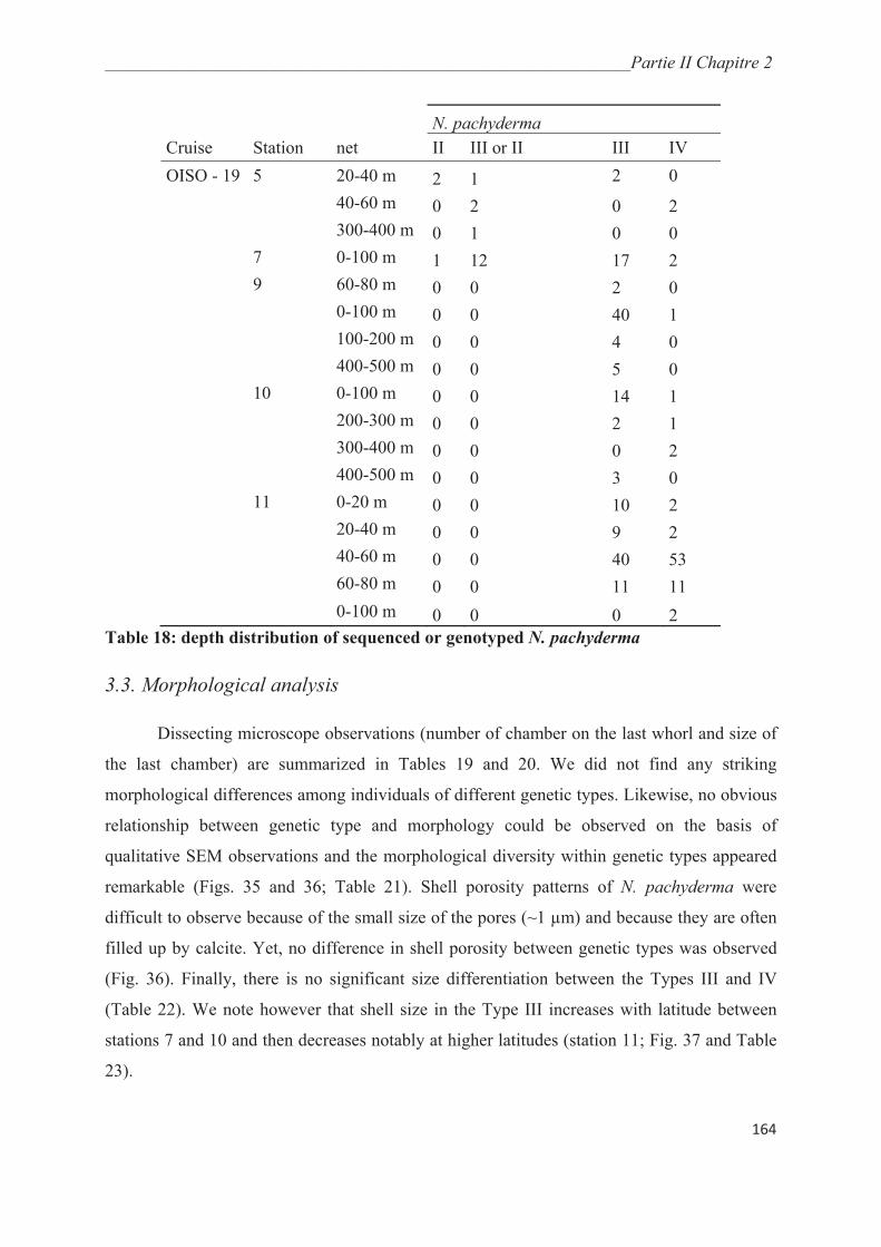
_______________________________________________________________________Partie II Chapitre 2
164
N. pachyderma
Cruise Station net II III or II III IV
OISO - 19 5 20-40 m 2 1 2 0
40-60 m 0 2 0 2
300-400 m 0 1 0 0
7 0-100 m 1 12 17 2
9 60-80 m 0 0 2 0
0-100 m 0 0 40 1
100-200 m 0 0 4 0
400-500 m 0 0 5 0
10 0-100 m 0 0 14 1
200-300 m 0 0 2 1
300-400 m 0 0 0 2
400-500 m 0 0 3 0
11 0-20 m 0 0 10 2
20-40 m 0 0 9 2
40-60 m 0 0 40 53
60-80 m 0 0 11 11
0-100 m 0 0 0 2
Table 18: depth distribution of sequenced or genotyped N. pachyderma
3.3. Morphological analysis
Dissecting microscope observations (number of chamber on the last whorl and size of
the last chamber) are summarized in Tables 19 and 20. We did not find any striking
morphological differences among individuals of different genetic types. Likewise, no obvious
relationship between genetic type and morphology could be observed on the basis of
qualitative SEM observations and the morphological diversity within genetic types appeared
remarkable (Figs. 35 and 36; Table 21). Shell porosity patterns of N. pachyderma were
difficult to observe because of the small size of the pores (~1 μm) and because they are often
filled up by calcite. Yet, no difference in shell porosity between genetic types was observed
(Fig. 36). Finally, there is no significant size differentiation between the Types III and IV
(Table 22). We note however that shell size in the Type III increases with latitude between
stations 7 and 10 and then decreases notably at higher latitudes (station 11; Fig. 37 and Table
23).

_______________________________________________________________________Partie II Chapitre 2
165
Kummerforms Normalforms
cruise station total type II type III type IV total type II type III type IV
OISO-19 5 1 0 1 0 6 1 4 1
OISO-19 7 1 0 1 0 19 1 16 2
OISO-19 9 4 0 3 1 44 0 44 0
OISO-19 10 5 0 4 1 17 0 14 3
OISO-19 11 9 0 7 2 114 0 53 61
OISO-21 6 4 1 3 0 19 1 18 0
OISO-21 7 5 3 2 0 21 6 15 0
OISO-21 8 6 0 6 0 30 2 28 0
OISO-21 9 14 0 14 0 74 0 74 0
OISO-21 10 13 0 13 0 86 0 86 0
OISO-21 11 8 0 7 1 75 0 56 19
Table 19: size of the last chamber and Neogloboquadrina pachyderma genetic types
4 to 4.5-chambers 4.5 to 5-chambers
cruise station total type II type III type IV total type II type III type IV
OISO-19 5 4 0 2 2 3 1 2 0
OISO-19 7 5 1 4 0 15 0 13 2
OISO-19 9 21 0 19 2 17 0 15 2
OISO-19 10 14 0 11 3 5 0 4 1
OISO-19 11 77 0 37 40 11 0 7 4
OISO-21 6 5 0 5 0 6 2 4 0
OISO-21 7 9 4 5 0 7 3 4 0
OISO-21 8 16 0 16 0 9 1 8 0
OISO-21 9 18 0 18 0 36 0 36 0
OISO-21 10 34 0 34 0 23 0 23 0
OISO-21 11 35 0 24 11 9 0 7 2
Table 20: number of chambers on the last whorl and Neogloboquadrina pachyderma
genetic types

_______________________________________________________________________Partie II Chapitre 2
166
Figure 35: scanning electronic microscope (SEM) pictures of representatives of the
Types II and III of Neogloboquadrina pachyderma collected during the OISO-19 cruise.
Genetic types and sampling locations are summarized in Table 21.

_______________________________________________________________________Partie II Chapitre 2
167
Figure 36: scanning electronic microscope pictures of representatives of the Types IV of
Neogloboquadrina pachyderma and non-genotyped/sequenced specimens collected
during the cruise OISO-19 (a-z). Genetic types and sampling locations are summarized
in Table 21. IVa and b: photomicrographs of the shell surface of the Type IV of N.
pachyderma. III a and b: photomicrographs of the shell surface of the Type III of N.
pachyderma. Scale bar = 5 μm.
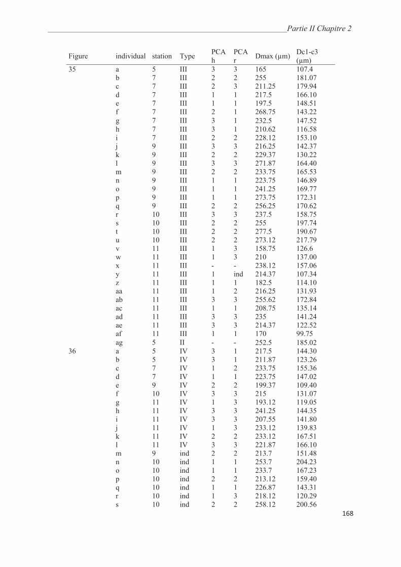
_______________________________________________________________________Partie II Chapitre 2
168
Figure individual station Type PCA
h
PCA
r Dmax (μm)
Dc1-c3
(μm)
35 a 5 III 3 3 165 107.4
b 7 III 2 2 255 181.07
c 7 III 2 3 211.25 179.94
d 7 III 1 1 217.5 166.10
e 7 III 1 1 197.5 148.51
f 7 III 2 1 268.75 143.22
g 7 III 3 1 232.5 147.52
h 7 III 3 1 210.62 116.58
i 7 III 2 2 228.12 153.10
j 9 III 3 3 216.25 142.37
k 9 III 2 2 229.37 130.22
l 9 III 3 3 271.87 164.40
m 9 III 2 2 233.75 165.53
n 9 III 1 1 223.75 146.89
o 9 III 1 1 241.25 169.77
p 9 III 1 1 273.75 172.31
q 9 III 2 2 256.25 170.62
r 10 III 3 3 237.5 158.75
s 10 III 2 2 255 197.74
t 10 III 2 2 277.5 190.67
u 10 III 2 2 273.12 217.79
v 11 III 1 3 158.75 126.6
w 11 III 1 3 210 137.00
x 11 III - - 238.12 157.06
y 11 III 1 ind 214.37 107.34
z 11 III 1 1 182.5 114.10
aa 11 III 1 2 216.25 131.93
ab 11 III 3 3 255.62 172.84
ac 11 III 1 1 208.75 135.14
ad 11 III 3 3 235 141.24
ae 11 III 3 3 214.37 122.52
af 11 III 1 1 170 99.75
ag 5 II - - 252.5 185.02
36 a 5 IV 3 1 217.5 144.30
b 5 IV 3 1 211.87 123.26
c 7 IV 1 2 233.75 155.36
d 7 IV 1 1 223.75 147.02
e 9 IV 2 2 199.37 109.40
f 10 IV 3 3 215 131.07
g 11 IV 1 3 193.12 119.05
h 11 IV 3 3 241.25 144.35
i 11 IV 3 3 207.55 141.80
j 11 IV 1 3 233.12 139.83
k 11 IV 2 2 233.12 167.51
l 11 IV 3 3 221.87 166.10
m 9 ind 2 2 213.7 151.48
n 10 ind 1 1 253.7 204.23
o 10 ind 1 1 233.7 167.23
p 10 ind 2 2 213.12 159.40
q 10 ind 1 1 226.87 143.31
r 10 ind 1 3 218.12 120.29
s 10 ind 2 2 258.12 200.56
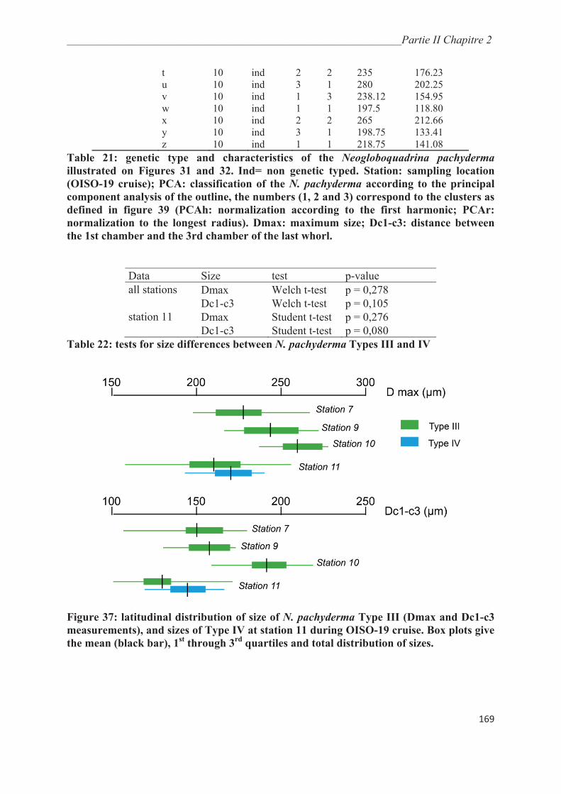
_______________________________________________________________________Partie II Chapitre 2
169
t 10 ind 2 2 235 176.23
u 10 ind 3 1 280 202.25
v 10 ind 1 3 238.12 154.95
w 10 ind 1 1 197.5 118.80
x 10 ind 2 2 265 212.66
y 10 ind 3 1 198.75 133.41
z 10 ind 1 1 218.75 141.08
Table 21: genetic type and characteristics of the Neogloboquadrina pachyderma
illustrated on Figures 31 and 32. Ind= non genetic typed. Station: sampling location
(OISO-19 cruise); PCA: classification of the N. pachyderma according to the principal
component analysis of the outline, the numbers (1, 2 and 3) correspond to the clusters as
defined in figure 39 (PCAh: normalization according to the first harmonic; PCAr:
normalization to the longest radius). Dmax: maximum size; Dc1-c3: distance between
the 1st chamber and the 3rd chamber of the last whorl.
Data Size test p-value
all stations Dmax Welch t-test p = 0,278
Dc1-c3 Welch t-test p = 0,105
station 11 Dmax Student t-test p = 0,276
Dc1-c3 Student t-test p = 0,080
Table 22: tests for size differences between N. pachyderma Types III and IV
Figure 37: latitudinal distribution of size of N. pachyderma Type III (Dmax and Dc1-c3
measurements), and sizes of Type IV at station 11 during OISO-19 cruise. Box plots give
the mean (black bar), 1st through 3
rd quartiles and total distribution of sizes.
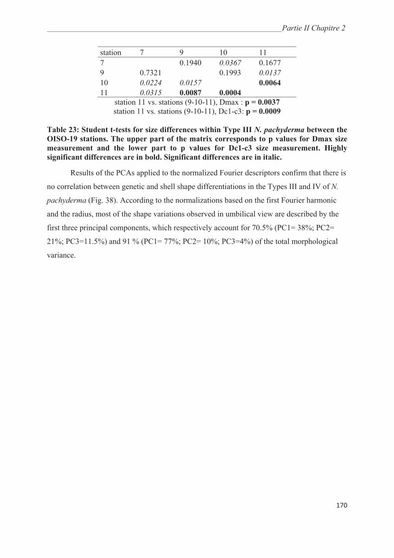
_______________________________________________________________________Partie II Chapitre 2
170
station 7 9 10 11
7 0.1940 0.0367 0.1677
9 0.7321 0.1993 0.0137
10 0.0224 0.0157 0.0064
11 0.0315 0.0087 0.0004
station 11 vs. stations (9-10-11), Dmax : p = 0.0037
station 11 vs. stations (9-10-11), Dc1-c3: p = 0.0009
Table 23: Student t-tests for size differences within Type III N. pachyderma between the
OISO-19 stations. The upper part of the matrix corresponds to p values for Dmax size
measurement and the lower part to p values for Dc1-c3 size measurement. Highly
significant differences are in bold. Significant differences are in italic.
Results of the PCAs applied to the normalized Fourier descriptors confirm that there is
no correlation between genetic and shell shape differentiations in the Types III and IV of N.
pachyderma (Fig. 38). According to the normalizations based on the first Fourier harmonic
and the radius, most of the shape variations observed in umbilical view are described by the
first three principal components, which respectively account for 70.5% (PC1= 38%; PC2=
21%; PC3=11.5%) and 91 % (PC1= 77%; PC2= 10%; PC3=4%) of the total morphological
variance.
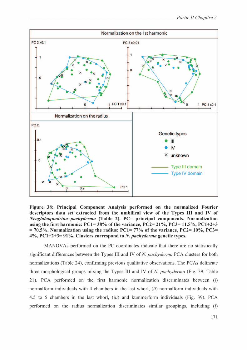
_______________________________________________________________________Partie II Chapitre 2
171
Figure 38: Principal Component Analysis performed on the normalized Fourier
descriptors data set extracted from the umbilical view of the Types III and IV of
Neogloboquadrina pachyderma (Table 2). PC= principal components. Normalization
using the first harmonic: PC1= 38% of the variance, PC2= 21%, PC3= 11.5%, PC1+2+3
= 70.5%. Normalization using the radius: PC1= 77% of the variance, PC2= 10%, PC3=
4%, PC1+2+3= 91%. Clusters correspond to N. pachyderma genetic types.
MANOVAs performed on the PC coordinates indicate that there are no statistically
significant differences between the Types III and IV of N. pachyderma PCA clusters for both
normalizations (Table 24), confirming previous qualitative observations. The PCAs delineate
three morphological groups mixing the Types III and IV of N. pachyderma (Fig. 39; Table
21). PCA performed on the first harmonic normalization discriminates between (i)
normalform individuals with 4 chambers in the last whorl, (ii) normalform individuals with
4.5 to 5 chambers in the last whorl, (iii) and kummerform individuals (Fig. 39). PCA
performed on the radius normalization discriminates similar groupings, including (i)
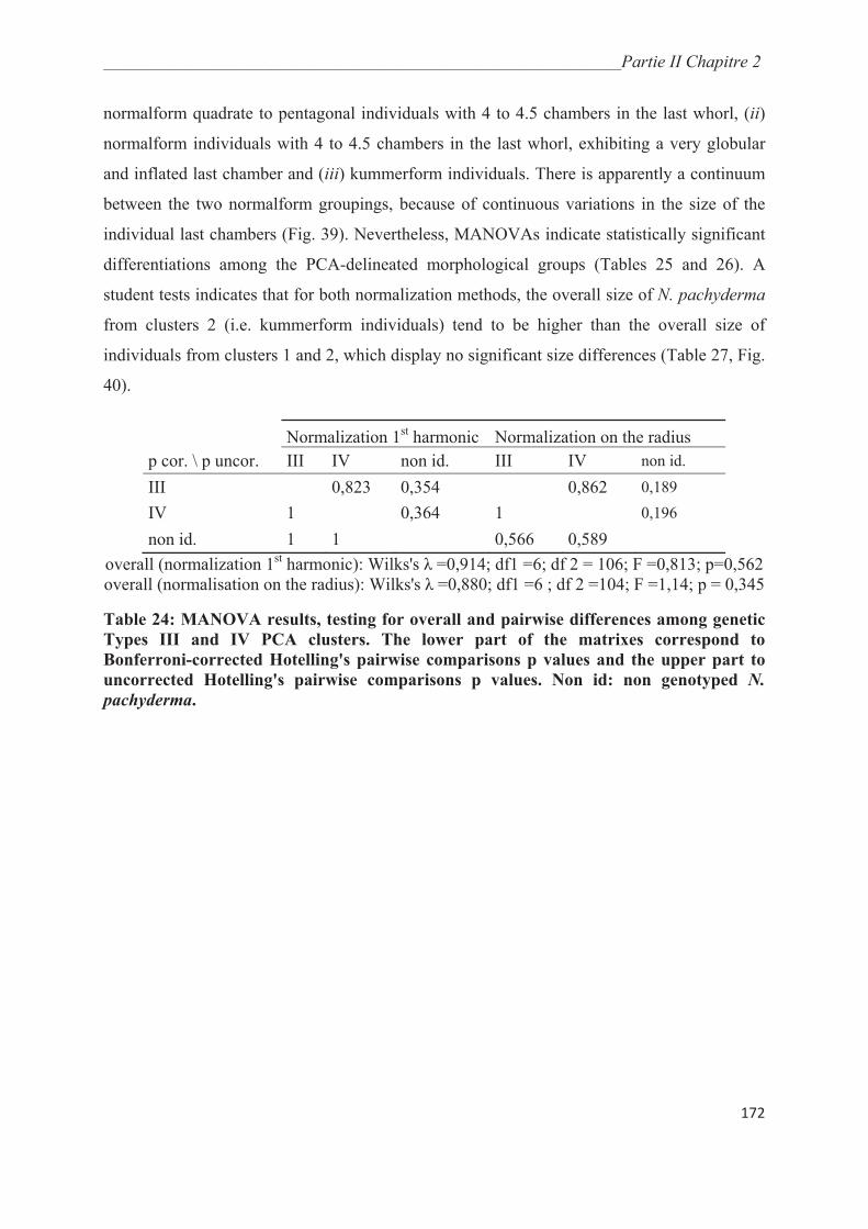
_______________________________________________________________________Partie II Chapitre 2
172
normalform quadrate to pentagonal individuals with 4 to 4.5 chambers in the last whorl, (ii)
normalform individuals with 4 to 4.5 chambers in the last whorl, exhibiting a very globular
and inflated last chamber and (iii) kummerform individuals. There is apparently a continuum
between the two normalform groupings, because of continuous variations in the size of the
individual last chambers (Fig. 39). Nevertheless, MANOVAs indicate statistically significant
differentiations among the PCA-delineated morphological groups (Tables 25 and 26). A
student tests indicates that for both normalization methods, the overall size of N. pachyderma
from clusters 2 (i.e. kummerform individuals) tend to be higher than the overall size of
individuals from clusters 1 and 2, which display no significant size differences (Table 27, Fig.
40).
Normalization 1st harmonic Normalization on the radius
p cor. \ p uncor. III IV non id. III IV non id.
III 0,823 0,354 0,862 0,189
IV 1 0,364 1 0,196
non id. 1 1 0,566 0,589
overall (normalization 1st harmonic): Wilks's =0,914; df1 =6; df 2 = 106; F =0,813; p=0,562
overall (normalisation on the radius): Wilks's =0,880; df1 =6 ; df 2 =104; F =1,14; p = 0,345
Table 24: MANOVA results, testing for overall and pairwise differences among genetic
Types III and IV PCA clusters. The lower part of the matrixes correspond to
Bonferroni-corrected Hotelling's pairwise comparisons p values and the upper part to
uncorrected Hotelling's pairwise comparisons p values. Non id: non genotyped N.
pachyderma.

_______________________________________________________________________Partie II Chapitre 2
173
Figure 39: Principal Component Analysis performed on the normalized Fourier
descriptors data set extracted from the umbilical view of the Types III and IV of
Neogloboquadrina pachyderma (Table 21) with normalization using the first harmonic
and normalization using the radius. PC= principal components. Clusters correspond to
PCA clusters and are linked to N. pachyderma morphological characteristics.
p cor. \ p uncor. Kumm Nor n<4,5 Nor 4,5< n<
4,75 Nor n> 4,75
Kumm 3,68E-14 4,05E-09 1,06E-05
Nor n<4,5 2,21E-13 5,11E-09 0,149052
Nor 4,5< n< 4,75 2,43E-08 3,07E-08 1,05E-04
Nor n> 4,75 6,36E-05 0,894312 6,33E-04
overall: Wilks's = 0,084 ; df1 = 9 ; df 2 = 129,1 ; F = 25,43 ; p = 1,15E-24
Table 25: MANOVA results, testing for overall and pairwise differences between PCA
clusters, normalization on the 1st harmonic. The lower part of the matrixes corresponds
to Bonferroni-corrected Hotelling's pairwise comparison p values and the upper part to
uncorrected Hotelling's pairwise comparison p values. Significant values are in bold.
Kumm: kummerforms; Nor: normalforms; n=number of chambers on the last whorl
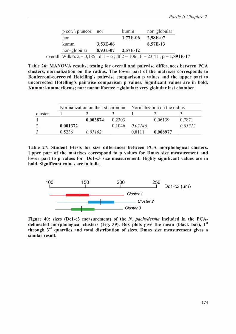
_______________________________________________________________________Partie II Chapitre 2
174
p cor. \ p uncor. nor kumm nor+globular
nor 1,77E-06 2,98E-07
kumm 3,53E-06 8,57E-13
nor+globular 8,93E-07 2,57E-12
overall: Wilks's = 0,185 ; df1 = 6 ; df 2 = 106 ; F = 23,41 ; p = 1,891E-17
Table 26: MANOVA results, testing for overall and pairwise differences between PCA
clusters, normalization on the radius. The lower part of the matrixes corresponds to
Bonferroni-corrected Hotelling's pairwise comparison p values and the upper part to
uncorrected Hotelling's pairwise comparison p values. Significant values are in bold.
Kumm: kummerforms; nor: normalforms; +globular: very globular last chamber.
Normalization on the 1st harmonic Normalization on the radius
cluster 1 2 3 1 2 3
1 0,003874 0,2303 0,06139 0,7871
2 0,001372 0,1046 0,02146 0,03512
3 0,5236 0,01162 0,8111 0,008977
Table 27: Student t-tests for size differences between PCA morphological clusters.
Upper part of the matrixes correspond to p values for Dmax size measurement and
lower part to p values for Dc1-c3 size measurement. Highly significant values are in
bold. Significant values are in italic.
Figure 40: sizes (Dc1-c3 measurement) of the N. pachyderma included in the PCA-
delineated morphological clusters (Fig. 39). Box plots give the mean (black bar), 1st
through 3rd
quartiles and total distribution of sizes. Dmax size measurement gives a
similar result.

_______________________________________________________________________Partie II Chapitre 2
175
4. Discussion
4.1. Collection methods
Most of recent studies focusing on morpho-genetic diversity in planktonic
foraminifera relied on a DNA sampling protocol which required individual sorting and careful
cleaning for on-board isolation in extraction buffer-filled PCR vials (Morard et al., 2009;
2011; 2013; Ujiié and Lipps, 2009; Ujiié et al., 2010; 2012; Aurahs et al., 2011; Quillévéré et
al., 2013). In the case of Neogloboquadrina pachyderma, this protocol is apparently not well
adapted for individual DNA conservation since we obtained very low (~40%) PCR success
rates when applied to the material collected during the cruise OISO-19, compared to success
rates obtained from other species of planktonic foraminifera (77 % for Orbulina universa, 70
% for Globigerinoides sacculifer, ~80 % for Globoconella inflata and Truncorotalia
truncatulinoides, R. Morard pers. comm.; André et al. [2013]). During the cruise OISO-21,
specimens were dried at fridge temperature right after collection and the PCR success rate
reached ~90% (Table 17). In this protocol, successfully used by Weiner et al. (2012),
foraminifers are quickly taken out of seawater which contains DNAses, while in the case of
the classical sampling protocol, it takes a longer time to put each single foraminifer in
individual buffer vials. Even using blue ice, it is difficult to avoid any increase in sample
seawater temperature when collecting in (sub)polar waters. We believe that these temperature
variations may have triggered DNA degradation reactions, thus explaining why PCR success
rates were so low when using this collection method. The “drying” protocol has the additional
advantages to reduce the collection time and to make easier any potential shipping, since the
samples are not stored within liquids.
4.2. Environmental controls on the distribution of genetic types of
Neogloboquadrina pachyderma in the Southern Ocean
Along the cruise transects OISO-19 and OISO-21, the Type II of N. pachyderma was
found north of the SAF, the Type IV represents 50% or more of the assemblages south of the
PF and the Type III was found to be cosmopolitan from temperate to polar waters (Fig. 32).
Comparison between years 2011 and 2012 shows that the distribution of these genetic types is
apparently influenced by the warming event that occurred in 2012, with in particular the Type
IV being less abundant and following the southward migration of the PF. The Type II was
_______________________________________________________________________Partie II Chapitre 2
176
apparently rarer in 2011 than in 2012 while there was virtually no temperature difference in
sub-polar sampled stations between the two years (Fig. 33). Consequently, temperature may
not be the sole environmental parameter controlling the distribution of the Type II. Primary
productivity may be involved as it was remarkably different between 2011 and 2012. During
the cruise OISO-19, the Type II was scarce while productivity was high, whereas during the
cruise OISO-21, this genetic type was four times more abundant and primary productivity was
lower. Furthermore, along the OISO-21 transect, we notice that the Type II was present at
stations 7 and 8 and not at station 9. Although 0-100 m depth temperatures were virtually the
same at these stations (Fig. 33), stations 7 and 8 correspond to low-productivity waters
whereas station 9 matches higher productivity values (Fig. 32). These observations, albeit
they would require confirmation through a further sampling of the Type II, suggest that this
genetic type inhabits warmer, lower-productivity waters than the Types III and IV. Likewise,
temperatures for station 10 were very similar in 2011 and 2012 and primary productivity was
higher during the cruise OISO 19; we found 4 specimens of the Type IV out of the 23
genotyped N. pachyderma in 2011 and none in 2012 although we genotyped 111 individuals.
Consequently, we hypothesize that the Type IV favors cold and productive austral waters.
Due to the Antarctic Circumpolar Current, the distribution of the genetic types of N.
pachyderma was expected to be similar in the south Indian and south Atlantic Oceans
(Darling et al., 2004). As shown in Figure 41, sampling stations in the south Atlantic along
the Cruises JR-19 (March 1997) and JR-48 transects (April 2000) follow similar temperature
gradients from sub-polar to polar waters, and in both cases, vertical temperature stratification
is weak in the first 100 m of the water column. Although the distribution of genetic types
appears globally similar along OISO and JR transects, some differences occur with, in the
south Atlantic, a higher relative abundance of the Type II and a restriction of the Type IV to
the Polar Frontal Zone (Figs. 32 and 41). Three hypotheses may explain these differences.
First, we note that JR sampling occurred in the austral autumn; as pointed by Norris (2000),
cryptic species may shift in the timing of reproduction and, as a consequence, may show
differences of population density with seasonality. This phenomenon was evidenced in the
case of Globigerinoides ruber (Aurahs et al., 2009) and Globigerina bulloides (Darling et al.,
2003). Consequently, the Type II of N. pachyderma may reproduce later than the Type III.
Second, in the South Atlantic, Darling et al. (2004) almost exclusively collected their material
in surface waters whereas in the South Indian Ocean, we collected material within the entire
_______________________________________________________________________Partie II Chapitre 2
177
depth range (0-100 m, Fig. 34) of N. pachyderma. Stratified sampling at station 11 of OISO-
19 shows that the Type III is more abundant in shallower waters than the Type IV.
Consequently, abundances of the Type III in polar waters of the South Atlantic may have
been overestimated. Unfortunately, our data are not sufficient to test whether the Type II is
indeed more abundant in warmer and low productivity surface waters than in deeper waters.
Third, these differences may result from differences in primary productivity occurring in the
studied regions. According to the distribution patterns observed in the south Indian Ocean, the
Type II favors decreasing primary productivity values. Although fluorescence profiles were
not recorded during the cruises JR, we speculate that higher abundances of the Type II in the
South Atlantic may reflect less eutrophic conditions during sampling period.
Figure 41: distribution of the Types II, III and IV of Neogloboquadrina pachyderma along
temperature profiles (0-100 m and 0-1000 m) crossed during the JR cruises in the southern
Atlantic Ocean reconstructed from Darling et al. (2004) and the World Ocean Database Atlas.
n= number of sequenced N. pachyderma (Darling et al., 2004), SAF: sub-Antarctic front; PF:
polar front. A: western transect of JR-48 cruise (Fig. 29). B: Eastern transect of JR-48 cruise
(Fig. 29). C: JR-19 transect (Fig. 29), with detail of the Antarctic zone.
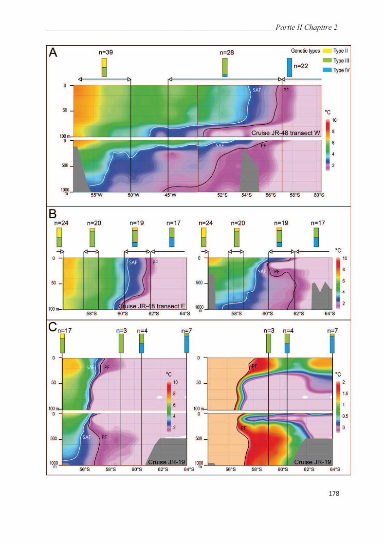
_______________________________________________________________________Partie II Chapitre 2
178
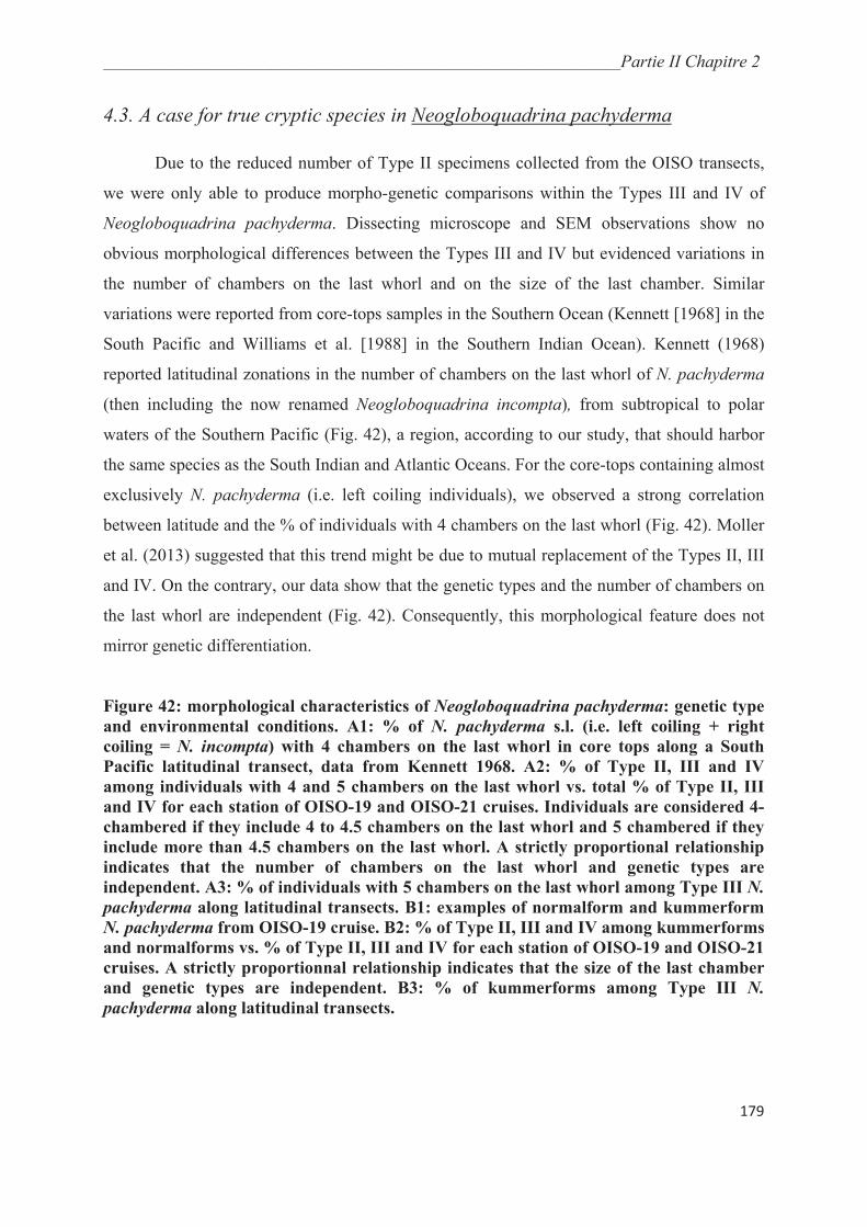
_______________________________________________________________________Partie II Chapitre 2
179
4.3. A case for true cryptic species in Neogloboquadrina pachyderma
Due to the reduced number of Type II specimens collected from the OISO transects,
we were only able to produce morpho-genetic comparisons within the Types III and IV of
Neogloboquadrina pachyderma. Dissecting microscope and SEM observations show no
obvious morphological differences between the Types III and IV but evidenced variations in
the number of chambers on the last whorl and on the size of the last chamber. Similar
variations were reported from core-tops samples in the Southern Ocean (Kennett [1968] in the
South Pacific and Williams et al. [1988] in the Southern Indian Ocean). Kennett (1968)
reported latitudinal zonations in the number of chambers on the last whorl of N. pachyderma
(then including the now renamed Neogloboquadrina incompta), from subtropical to polar
waters of the Southern Pacific (Fig. 42), a region, according to our study, that should harbor
the same species as the South Indian and Atlantic Oceans. For the core-tops containing almost
exclusively N. pachyderma (i.e. left coiling individuals), we observed a strong correlation
between latitude and the % of individuals with 4 chambers on the last whorl (Fig. 42). Moller
et al. (2013) suggested that this trend might be due to mutual replacement of the Types II, III
and IV. On the contrary, our data show that the genetic types and the number of chambers on
the last whorl are independent (Fig. 42). Consequently, this morphological feature does not
mirror genetic differentiation.
Figure 42: morphological characteristics of Neogloboquadrina pachyderma: genetic type
and environmental conditions. A1: % of N. pachyderma s.l. (i.e. left coiling + right
coiling = N. incompta) with 4 chambers on the last whorl in core tops along a South
Pacific latitudinal transect, data from Kennett 1968. A2: % of Type II, III and IV
among individuals with 4 and 5 chambers on the last whorl vs. total % of Type II, III
and IV for each station of OISO-19 and OISO-21 cruises. Individuals are considered 4-
chambered if they include 4 to 4.5 chambers on the last whorl and 5 chambered if they
include more than 4.5 chambers on the last whorl. A strictly proportional relationship
indicates that the number of chambers on the last whorl and genetic types are
independent. A3: % of individuals with 5 chambers on the last whorl among Type III N.
pachyderma along latitudinal transects. B1: examples of normalform and kummerform
N. pachyderma from OISO-19 cruise. B2: % of Type II, III and IV among kummerforms
and normalforms vs. % of Type II, III and IV for each station of OISO-19 and OISO-21
cruises. A strictly proportionnal relationship indicates that the size of the last chamber
and genetic types are independent. B3: % of kummerforms among Type III N.
pachyderma along latitudinal transects.
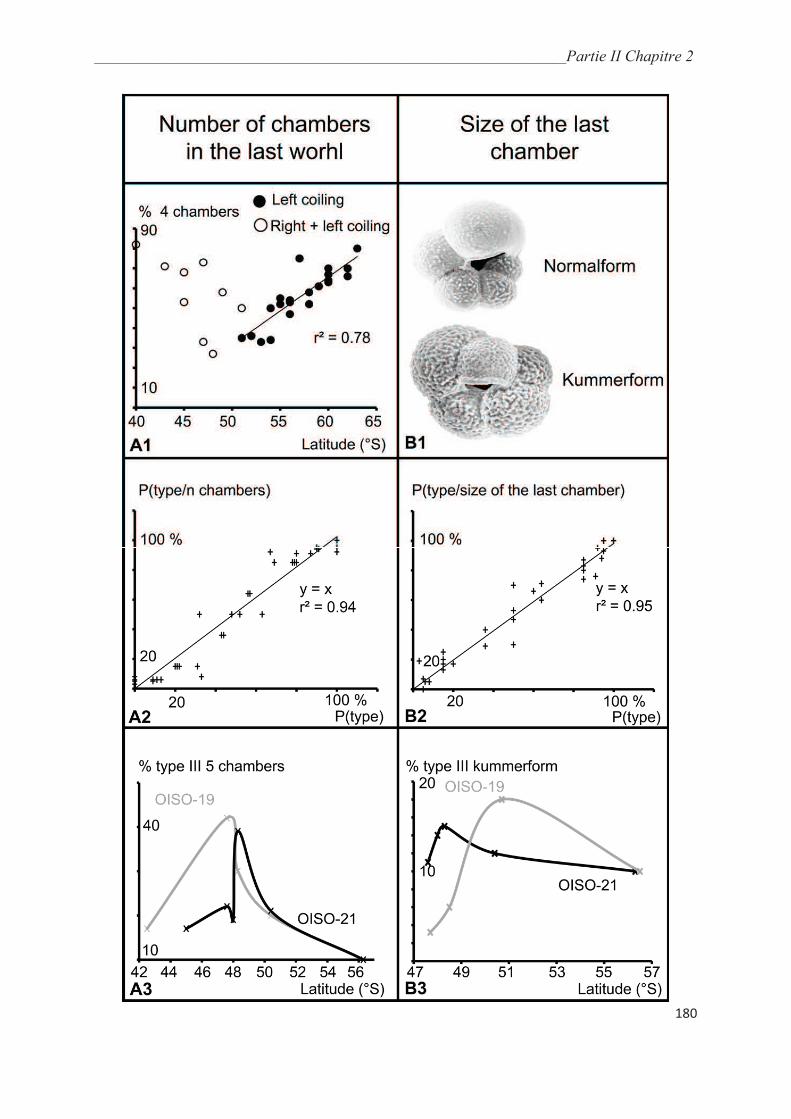
_______________________________________________________________________Partie II Chapitre 2
180
_______________________________________________________________________Partie II Chapitre 2
181
Along the OISO transects, we collected fewer kummerform specimens of the Type IV
than of the Type III (Table 19). The Type III being apparently more prone to diminutive last
chambers than the Type IV, we tested whether this morphological feature could reflect
genetic differentiation. Our data show that there is no correlation between the size of the last
chamber and genetic identity (Fig. 42). This conclusion is strengthened by the fact that in
southernmost Antarctic core-tops, a region only inhabited by the Type IV (Darling et al.
2004), kummerform N. pachyderma are common place (Norris et al., 1998).
Different genetic types of Globigerinella siphonifera and Orbulina universa were
distinguished thanks to significant differences in shell porosity (Huber et al., 1997; Morard et
al., 2009). Our observations suggest that it is not the case for the Types III and IV of N.
pachyderma. In N. pachyderma from the Ross Sea, a polar region inhabited only by the Type
IV, Bergami et al. (2009) showed that pore sizes and shell surface encrustation varies greatly
through calcification processes. Ultrastructural features are thus not putative criteria for
distinguishing the genetic types of N. pachyderma as they are difficult to observe and
probably vary greatly between ontogenetic stages.
Based on shell outline analyses performed on N. pachyderma and N. incompta
collected in core-top samples, Healy-Williams (1984) evidenced the occurrence of multiple
morphotypes in the South Indian Ocean. The distribution patterns of some of these
morphotypes may be correlated with salinity and/or sea surface temperatures but these
correlations are subject to caution since the author, in her analysis, considered N. pachyderma
and N. incompta as a single species. She sampled a latitudinal transect from 38°S to 65°S,
which includes the latitudes of our OISO transects, and consequently analyzed altogether
specimens of N. incompta and of the Types II, III and IV of N. pachyderma. Williams et al.
(1988) suggested that these morphotypes may constitute distinct species or sub-species. Our
PCA analysis performed on shell outlines delimits clusters (Fig. 39) similar to those defined
by Healy-Williams; our clusters 1, 2 and 3 corresponding to the morphotypes “Harmonic4”,
“Harmonic 5&6” and “Harmonic 3”, respectively. Our PCA shows that these morphological
variations do not match genetic differences as shell outlines of the Type III and Type IV are
not differentiated (Fig. 38).
_______________________________________________________________________Partie II Chapitre 2
182
It appears that the Types III and IV of N. pachyderma cannot be identified through the
set of morphological features investigated here and thus constitute true cryptic species. This
result was unexpected since genetic divergence between these genetic types is important and
their status as separate species unchallenged (André et al., in prep for reviews). Indeed, recent
morpho-genetic comparisons in planktonic foraminifera demonstrated that the most divergent
genetic types within a morphospecies exhibit significant differences in shell morphology,
which can be recognized based on population-scale morphometric analyses (de Vargas et al.,
2001; Morard et al., 2009; 2011; Aurahs et al., 2011; Quillévéré et al., 2013). As a
consequence, it seemed feasible to transfer the biological information acquired through
genetic analysis to paleoceanography, in peculiar by improving the resolving power of the
transfer functions that allow reconstructing past sea surface temperatures (Morard et al.,
2013). In the case of the (sub)polar Types III and IV of N. pachyderma, such transfer appears
to be unrealistic and their contrasted environmental affinities are of no use for improving
reconstructions in the Southern Ocean.
4.4. Ecophenotypic variations in genetic types of Neogloboquadrina
pachyderma
PCA sorting of individuals is linked to the size of the last chamber and the number of
chambers on the last whorl (Fig. 39). In particular, individuals were sorted according to the
size of the last chamber (normalforms vs. kummerforms) and, among normalforms, the PCA
set apart individuals according to the number of chambers on the last whorl. As a conclusion,
shell shapes of southern Ocean N. pachyderma are highly variable and mainly controlled by
the size of the last chamber and the number of chambers on the last whorl. Since this PCA
sorting does not correspond to genetic type clusters, these morphological features are not
linked with genetic diversity and thus possibly correspond to eco-phenotypic variations.
For the Type III of N. pachyderma, our study benefits a large number of collected specimens
along an extended latitudinal transect, then allowing us to analyze morphological changes
associated with environmental parameters within this genetic type. Mean shell size varies with
latitude (Fig. 37, Table 23) and reaches a maximum in the southernmost sub-polar waters of
our transects, at locations where this genetic type is most abundant (OISO-19, stations 9 and
10). These locations thus probably correspond to the ecological optimum (Ricklef, 1976;
Begon et al., 1986) of the Type III. We notice that at polar station 11, shell sizes of the Type
_______________________________________________________________________Partie II Chapitre 2
183
III and IV are reduced and not significantly different. This observation reinforces the
hypothesis that the Types III and IV of N. pachyderma reach their ecological optima further
north and further south of the station, respectively. A similar phenomenon was evidenced by
Moller et al. (2013) in the case of the Type I of N. pachyderma in the Atlantic Ocean.
Consequently, the size of N. pachyderma is an eco-phenotypic feature, with, for each genetic
type, larger shells corresponding to their ecological optimum. Therefore, the concept of Hecht
(1976) that planktonic foraminiferal morpho-species achieve largest sizes at their ecological
optima may also apply at the genetic type level.
Our data show that the % of 5-chambered specimens of the Type III follow a bell-
shaped curve with highest values reached at sub-polar latitudes (Fig. 42) within the ecological
optimum of this genetic type. Although we acknowledge that the number of collected
specimens of the Types II and IV remains still limited, shell size distributions of these genetic
types apparently follow the same pattern. Indeed, the % of 5-chambered specimens of
temperate to sub-polar Type II decreases southwards whereas that of the polar Type IV
increases (Table 20). In the Southern Ocean, there is likely an ecophenotypic variation in the
number of chambers on the last whorl in N. pachyderma, with increasing values at ecological
optima. This observation may be generalized to the other genetic types of N. pachyderma
elsewhere in the world Oceans. In the North West Pacific, where only the Type VII
apparently occurs (Darling et al., 2007), Khan (1981) evidenced a relationship between the
preferred depth of N. pachyderma and the abundance of 5-chambered specimens.
The size of the last chamber exhibits similar patterns of variation with environmental
data. In the Type III, the % of kummerform specimens follows a bell shaped curve with
highest values reached at sub-polar latitudes within the ecological optimum of the genetic
type (Fig. 42). Similarly, abundance of kummerform specimens of the Type II apparently
decreases with latitude in temperate to sub-polar waters when that of the Type IV apparently
increases in polar waters (Table 19), then suggesting that the pattern evidenced in the Type III
may be generalized to the other genetic types of N. pachyderma. In cryptic species of N.
pachyderma from the Southern Ocean, the size of the last chamber is consequently an
ecophenotypic feature with maximum abundances of kummerform specimens reached at
ecological optima. A reduced final chamber is unlikely to reflect environmental stress as
suggested by Hecht and Savin (1970) but rather an indication of maximal growth achievement
as advocated by Olsson (1973). Such ecophenotypic variation may explain why fewer Type
IV kummerforms specimens were sampled in the South Indian Ocean than in the South
_______________________________________________________________________Partie II Chapitre 2
184
Atlantic (Table 19; Fig. 39). During the OISO collecting transects, the ecological optimum of
the polar Type IV, which is probably located further south in extreme Antarctic waters
(Darling et al., 2004) where kummerform N. pachyderma are particularly abundant (Norris et
al., 1998), was not sampled. We conclude that shell morphology variations (size, number of
chambers on the last whorl and size of the last chamber) in the Types III and IV of N.
pachyderma are eco-phenotypic. These genetic types show that the assumption that
morphological variations reflect genetic diversity with planktonic foraminifera (Huber et al.,
1997; de Vargas et al., 2001; Morard et al., 2009; 2011; Aurahs et al., 2011; Quillévéré et al.,
2013) is not a general rule. Generalization was indeed hasty as, until now, precise
morphological variations of genetic types where studied for only a 5 out of the 13 morpho-
species for which cryptic diversity have been evidenced (André et al., in prep for reviews;
Huber et al., 1997; de Vargas et al., 2001; Morard et al., 2009; 2011; Aurahs et al., 2011;
Quillévéré et al., 2013). Furthermore, the case of Globigerinoides sacculifer showed that
morphological plasticity within a single genetic type can be significant. Consequently,
morpho-genetic analyses may reveal other exceptions than the genetic types of N.
pachyderma.
_______________________________________________________________________Partie II Chapitre 2
185
5. Conclusions
In the south Indian Ocean, distributions of cryptic species of Neogloboquadrina
pachyderma are similar to those previously observed in the South Atlantic (Darling et al.,
2004. These distributions are apparently correlated to the latitudinal sea surface temperature
gradient but primary productivity also plays a key role, particularly for the distribution of the
Type II. At sub-polar to polar latitudes, the Type III is sympatric with the Types II or IV. As
cryptic species rarely share the same environmental niche (Zhang et al., 2004), this may imply
different depth habitats and/or diets or differences in reproduction timing (Norris et al., 2000).
Neither precise feeding behaviors nor seasonality of genetic types of N. pachyderma could be
investigated, but, even if our data on depth stratification is still largely insufficient to
conclude, we evidence possible depth partitioning of the Types III and IV linked to primary
productivity. Differences in depth habitats between the Types II, III and IV are thus likely and
may explain the slight distribution differences between our results and those obtained by
Darling et al. (2004) in the South Atlantic.
Unexpectedly, the extensive morphological variability in N. pachyderma does not
reflect its genetic diversity. The Types III and IV of N. pachyderma are the first demonstrated
cases of true cryptic species in planktonic foraminifera. Morphological characteristics of these
genetic types are clearly eco-phenotypic. In particular, whenever individuals are at their
genetic type ecological optimum, they tend to be larger, to have 5 chambers on the last whorl
and to exhibit a reduced final chamber (kummerform). The study of Eynaud et al. (2009) on
the arctic genetic Type I of N. pachyderma also evidenced a high morphological variability,
suggesting that shell morphology may be principally controlled by the environmental
conditions within the entire morphospecies. This was unexpected as true cryptic species are
considered as rare in the pelagic domain (Knowlton, 1993) and as, so far, previously defined
planktonic foraminifera eco-phenotypes turned out to be distinct genetic types (de Vargas et
al., 2001; Morard et al., 2009; 2011; Aurahs et al., 2011; Quillévéré et al., 2013). This study
reminds that speciation is not always accompanied by morphological changes (e.g. Elmer et
al., 2007). Indeed, for planktonic foraminifera, morphological recognition plays no role in
same species individuals or gametes recognition. Mate-choice systems may rely on non-
morphological characteristics such as chemical signals that are difficult to establish for rarely
cultivated organisms (Knowlton, 1993; Bickford et al., 2006).

_______________________________________________________________________Partie II Chapitre 2
186
Acknowledgements
We thank L. Konecny, L. Rossignol, M-H. Castera and G. Isguder for technical
assistance. We acknowledge the assistance of the Master and the crew of the OISO cruises
during which the presented material has been collected. Special thanks are given to the Institut
Polaire Français Paul Emile Victor (IPEV). This work was supported by grants from the
Institut National des Sciences de l’Univers (INSU) INTERRVIE program (F.Q.).
Supplementary file
Principal component (PC) values. Fig_ind: figure_individual, name of the sample on the
corresponding figures (Figs 35 and 36, Table 21). The cluster numbers refers to figure 39.
___________________________________________________________Partie II Chapitre 2
187
References
André, A., Weiner, A., Quillévéré, F., Aurahs, R., Morard, R., Douady, C., de Garidel-
Thoron, T., Escarguel, G., de Vargas, C. and Kucera, M., 2013. The cryptic and the
apparent reversed: lack of genetic differentiation within the morphologically diverse
plexus of the planktonic foraminifer Globigerinoides sacculifer. Paleobiology, 39: 21-
39.
André, A., Quillévéré, F., Morard, R., de Vargas, C., Ujiié, Y., and Douady, C., in prep. SSU
rDNA divergence in planktonic foraminifera: molecular taxonomy and biogeographic
implications.
Aurahs, R., Grimm, G., Hemleben, V., Hemleben, C. and Kucera, M., 2009. Geographical
distribution of cryptic genetic types in the planktonic foraminifer Globigerinoides
ruber. Molecular Ecology, 18: 1692-1706.
Aurahs, R., Treis, Y., Darling, K. and Kucera, M., 2011. A revised taxonomic and
phylogenetic concept for the planktonic foraminifer species Globigerinoides ruber
based on molecular and morphometric evidence. Marine Micropaleontology, 79: 1-14.
Aze, T., Ezard, T., Purvis, T., Coxall, H., Stewart, D., Wade, B. and Pearson, P., 2011. A
phylogeny of Cenozoic macroperforate planktonic foraminifera from fossil data.
Biological Reviews 86: 900-927.
Bandy, O.L., 1972. Origin and development of Globorotalia (Turborotalia) pachyderma
(Ehrenberg). Micropaleontology, 18: 294-318.
Banner, F.T. and Blow, W.H., 1960. Some primary types of species belonging to the
superfamily Globigerinaceae. Contributions from the Cushman Foundation for
Foraminiferal Research, 11: 1–45.
Barker, S., Cacho, I., Benway, H. and Takachikawa, K., 2005. Planktonic foraminiferal
Mg/Ca as a proxy for past oceanic temperatures: a methodological overview and data
compilation for the Last Glacial Maximum. Quaternary Science Reviews, 24: 821-834.
Becquey, S. and Gersonde, R., 2003. A 0.55-Ma paleotemperature record from the
subantarctic zone: implications for Antarctic Circumpolar Current development.
Paleoceanography, 18: 1014-1028.
Begon, M., Harper, J.L. and Townsend, J.R., 1986. Ecology : individuals, populations and
communities. Blackwell Scientific Publications, Oxford.
Bergami, C., Capotondi, L., Langone, L., Giglio, F. and Ravaioli, M., 2009. Distribution of
living planktonic foraminifera in the Ross Sea and the Pacific sector of the Southern
Ocean (Antarctica). Marine Micropaleontology, 73: 37-48.
Berger, W.H., 1969. Planktonic foraminifera: basic morphology and ecologic implications.
Journal of paleontology, 43: 1369-1383.
Bickford, D., Lohman, D.J., Sodhi, N.S., Ng, P.K.L., Meier, R., Winker, K., Ingram, K.K. and
Das, I., 2007. Cryptic species as a window on diversity and conservation. Trends in
Ecology and Evolution, 22:148–155.

___________________________________________________________Partie II Chapitre 2
188
Broecker, W.S., 1982. Ocean chemistry during glacial time. Geochimica et Cosmochimica
Acta, 46: 1689-1705.
Carter, L., McCave, I.N., Williams, M.J.M., Fabio, F. and Martin, S., 2008. Chapter 4
circulation and water masses of the Southern Ocean: a review. Developments in Earth
and Environmental Sciences, Elsevier, Amsterdam.
Cifelli, R., 1961. Globigerina incompta, a new species of pelagic foraminiera from the North
Atlantic Ocean. Contributions of the Cushman Foundation for Foraminiferal Research,
12: 83-86.
CLIMAP, 1981. Seasonnal reconstructions of the Earth's surface at the last glacial maximum.
Geological Society of Americain Map and Chart Series, MC-36.
Darling, K.F., Wade, C.M., Kroon, D. and Brown, A.J., 1997. Planktic foraminiferal
molecular evolution and their polyphyletic origins from benthic taxa. Marine
Micropaleontology, 30: 251–266.
Darling, K.F., Kucera, M., Wade, C.M., Langen, P.V. and Pak, D., 2003. Seasonal
distribution of genetic types of planktonic foraminifer morphospecies in the Santa
Barbara Channel and its paleoceanographic implications. Paleoceanography, 18: 1032-
1042.
Darling, K.F., Kucera, M., Pudsey, C.J. and Wade, C.M., 2004. Molecular evidence links
cryptic diversification in polar planktonic protists to Quaternary climate dynamics.
Proceedings of the National Academy of Science of the United States of America, 101:
7657-7662.
Darling, K.F., Kucera, M., Kroon, D. and Wade, C.M., 2006. A resolution for the coiling
direction paradox in Neogloboquadrina pachyderma. Paleoceanography, 21: 1-14.
Darling, K.F., Kucera, M. and Wade, C.M., 2007. Global molecular phylogeography reveals
persistent arctic circumpolar isolation in a marine planktonic protist. Proceedings of the
National Academy of Science of the United States of America, 104: 5002-5007.
Darling, K.F. and Wade, C.M., 2008. The genetic diversity of planktic foraminifera and the
global distribution of ribosomal RNA genotypes. Marine Micropaleontology, 67: 216-
238.
de Vargas, C., Norris, R.D., Zaninetti, L., Gibb, S.W. and Pawlowski, J., 1999. Molecular
evidence of cryptic speciation in planktonic foraminifers and their relation to oceanic
provinces. Proceedings of the National Academy of Sciences of the United Sates of
America, 96: 2864-2868.
de Vargas, C., Renaud, S., Hilbrecht, H. and Pawlowski, J., 2001. Pleistocene adaptive
radiation in Globorotalia truncatulinoides: genetic, morphologic, and environmental
evidence. Paleobiology, 27: 104-125.
de Vernal., A. and Hillaire-Marcel, C., 2006. Provincialism in trends and high frequency
change in the northwest North Atlantic during the Holocene. Global Planetary Change,
54: 263-290.
Dieckmann, G.S., Spindler, M., Mange, M.A., Ackley, S.F. and Eicken, H., 1991. Antarctic
sea ice: a habitat for the foraminifer Neogloboquadrina pachyderma. Journal of
Foraminiferal Research, 21: 183-189.

___________________________________________________________Partie II Chapitre 2
189
Elmer, K., Davila, J. and Lougheed, S., 2007. Cryptic diversity and deep divergence in an
upper Amazonian leaflitter frog, Eleutherodactylus ockendeni. BioMed Central
Evolutionary Biology, 7: 247.
Ericson, D.B., 1959. Coiling direction of Globigerina pachyderma as a climatic index:
Science, 130: 219–220.
Eynaud, F., Cronin, T.M., Smith, S.A., Zaragosi, S., Mavel, J., Mary, Y, Mas, V. and Pujol,
C., 2009. Morphological variability of the planktonic foraminifer Neogloboquadrina
pachyderma from ACEX cores: implications for the Late Pleistocene circulation of the
Arctic Ocean. Micropaleontology, 55: 101-116.
Foote, M., 1989. Perimeter-based Fourier analysis: A new morphometric method applied to
the trilobite cranidium. Journal of Paleontology, 63: 880-885.
Hammer, Ø., Harper, D.A.T. and Ryan, P.D., 2001. PAST: Paleontological statistics software
package for education and data analysis. Palaeontologia Electronica, 4: 9.
Healy-Williams, N., 1984. Quantitative image analysis: application to planktonic
foraminiferal paleoecology and evolution. Geobios, 17: 425-432.
Hecht, A.D. and Savin, S.M., 1970. Oxygen-18 studies on recent planktonic foraminifera:
comparaison of phenotypes and test parts. Science, 170: 69.
Hecht, A.D., 1976. An ecologic model for test size variation in recent planktonic
foraminifera: applications to the fossil record. Journal of Foraminiferal Research, 6:
295-311.
Hemleben, C., Spindler, M. and Anderson, O.R., 1989. Modern Planktonic Foraminifera.
Springer, New York.
Huber, B.T., Bijma, J. and Darling, K.F., 1997. Cryptic speciation in the living planktonic
foraminifer Globigerinella siphonifera (d'Orbigny). Paleobiology, 23: 33-62.
Ikeda, Y., Siedler, G. and Zwierz, M., 1989. On the variability of the Southern Ocean Front
locations between Southern Brazil and the Antarctic Peninsula. Journal of Geophysical
Research, 94: 4757-4762.
Iwata, H. and Ukai, Y., 2002. SHAPE: A computer program package for quantitative
evaluation of biological shapes based on elliptic Fourier descriptors. Journal of
Heredity, 93: 384-385.
Kahn, M.I., 1981. Ecological and paleoecological implications of the phenotypic variation in
three species of living planktonic foraminifera from the northeastern Pacific Ocean
(50°N, 145°W). Journal of Foraminiferal Research, 11: 203-211.
Katz, M.E., Crammer, B.S., Franzese, A., Barbel, H., Miller, K.G., Rosenthal, Y. and Wright,
J.D., 2010. Traditional and merging geochemical proxies in foraminifera. Journal of
Foraminiferal Research, 40: 165-192.
Keir, R.S., 1988. On the Late Pleistocene ocean geochemistry and circulation.
Paleoceanography, 3: 413-445.
Kennett, J.P., 1968. Latitudinal variation in Globigerina pachyderma (Ehrenberg) in surface
sediments of the Southwest Pacific Ocean. Micropaleontology, 14: 305-318.
___________________________________________________________Partie II Chapitre 2
190
Kennett, J.P. and Srinivasan, M.S., 1983. Neogene Planktonic Foraminifera: a Phylogenetic
Atlas. Hutchinson Ross, Sroudsburg (Pennsylvania).
Knowlton, N., 1993. Sibling species in the sea. Annual Review of Ecology and Systematics,
24: 189-216.
Kucera, M. and Darling, K.F., 2002. Cryptic species of planktonic foraminifera: their effect
on palaeoceanographic reconstructions. Philosophical Transaction of the Royal Society
of London, 360: 695-718.
Kucera, M., 2007. Planktonic foraminifera as tracers of past oceanic environments. Proxies in
Late Cenozoic Paleoceanography, Elsevier, Amsterdam.
Kuhl, F.P. and Giardina, C.R., 1982. Elliptic Fourier features of a closed contour. Computer
Graphics and Image Processing, 18: 236-258.
MARGO project members, 2009. Constraints on the magnitude and patterns of ocean cooling
at the last glacial maximum. Nature Geoscience, 2: 127-132.
Metzl, N., 2000. Le programme OISO, Service d'Observation de l'Océan Indien / The OISO
program: Observations in the Indian Ocean. Lettre Internationale Géosphere Biosphère
Programme, 10: 76-83.
Moller, T., Schulz, H. and Kucera, M., in press. The effect of sea surface properties on shell
morphology and size of the planktonic foraminifer Neogloboquadrina pachyderma in
the North Atlantic. Palaeogeography, Palaeoclimatology, Palaeoecology.
Morard, R., Quillévéré, F., Escarguel, G., Ujiie, Y., de Garidel-Thoron, T. Norris, R.D. and de
Vargas, C., 2009. Morphological recognition of cryptic species in the planktonic
foraminifer Orbulina universa. Marine Micropaleontology, 71: 148-165.
Morard, R., Quillévéré, F., Douady, C.J., de Vargas, C., de Garidel-Thoron, T. and Escarguel,
G., 2011.Worldwide Genotyping in the Planktonic Foraminifer Globoconella inflata:
Implications for Life History and Paleoceanography. Public Library of Science One, 6:
e26665.
Morard, R., Quillevere, F., Escarguel, G., de Garidel-Thoron, T., de Vargas, C. and Kucera,
M., 2013. Ecological modeling of the temperature dependence of cryptic species of
planktonic foraminifera in the Southern Hemisphere. Palaeogeography
Palaeoclimatology Palaeoecology. http://dx.doi.org/10.1016/j.palaeo.2013.05.011
Norris, R., Kim, D., Park, B.-K., Kang, S.-H. and Khim, B.-K., 1998. Stable isotope and
ecological habitat of planktonic foraminifera adjacent to the ice edge in the western
Weddell Sea. Geosciences Journal, 2: 88-98.
Norris, R.D., 2000. Pelagic species diversity, biogeography and evolution. Paleobiology, 26:
236-258.
Olsson, R.K., 1973. What is a kummerform planktonic foraminifer? Journal of Paleontology,
47: 327-329.
Pflaumann, U., Duprat, J., Pujol, C. and Labeyrie, L., 1996. SIMMAX: A modern analog
technique to deduce Atlantic sea surface temperatures from planktonic foraminifera in
deep-sea sediments. Paleoceanography, 11: 15-36.
Prell, W.L., Martin, A., Cullen, J.L. and Trend, M., 1999. The Brown University
Foraminiferal Data Base (BFD).
___________________________________________________________Partie II Chapitre 2
191
Quillévéré, F., Debat, V. and Auffray, J.-C., 2002. Ontogenetic and evolutionary patterns of
shape differentiation during the initial diversification of Paleocene acarininids
(planktonic foraminifera). Paleobiology, 28: 435-448.
Quillévéré, F., Morard, R., Escarguel, G., Douady, C.J., Ujiie, Y., de Garidel-Thoron, T. and
de Vargas, C., in press. Global scale same-specimen morpho-genetic analysis of
Truncorotalia truncatulinoides: A perspective on the morphological species concept in
planktonic foraminifera. Palaeogeography, Palaeoclimatology, Palaeoecology.
R Development Core Team, 2004. R: a language and environment for statistical computing.
Renaud, S. and Schmidt, D.N., 2003. Habitat tracking as a response of the planktic
foraminifer Globorotalia truncatulinoides to environmental fluctuations during the last
140 kyr. Marine Micropaleontology, 49: 97-122.
Ricklefs, R., 1976. The economy of nature: a textbook in basic ecology. Chiron, Portland.
Schlitzer, R., 2011. Ocean Data View. http://odv.awi.de
Ujiie, Y. and Lipps, J.H., 2009. Cryptic diversity in planktic foraminifera in the northwest
Pacific Ocean. Journal of Foraminiferal Research, 39: 145-154.
Ujiié, Y., de Garidel-Thoron, T., Watanabe, S., Wiebe, P. and de Vargas, C., 2010. Coiling
dimorphism within a genetic type of the planktonic foraminifer Globorotalia
truncatulinoides. Marine Micropaleontology, 77: 145-153.
Ujiie, Y., Asami, T., de Garidel-Thoron, T., Liu, H., Ishitani, Y. and de Vargas, C., 2012.
Longitudinal differentiation among pelagic populations in a planktic foraminifer.
Ecology and Evolution, 2: 1725-1737.
Weiner, A., Aurahs, R., Kurasawa, A., Kitazato, H. and Kucera, M., 2012. Vertical niche
partitioning between cryptic sibling species of a cosmopolitan marine planktonic protist.
Molecular Ecology, 21: 4063-4073.
Williams, D.F., Ehrlich, R., Spero, H.J., Healy-Williams, N. and Gary, A.C., 1988. Shape and
isotopic differences between conspecific foraminiferal morphotypes and resolution of
paleoceanographic events. Palaeogeography, Palaeoclimatology, Palaeoecology, 64:
153-162.
World Ocean Atlas 2009 (WOA09), http://www.nodc.noaa.gov/OC5/WOA09/pr_woa09.html
Zachos, J., Pagani, M., Sloan, L., Thomas, E. and Billups, K., 2001. Trends, rhythms, and
aberrations in global climate 65 Ma to present. Science, 292: 686-693.
Zhang, D.-Y., Lin, K. and Hanski, I., 2004. Coexistence of cryptic species. Ecology Letters,
7: 165-169.
_________________________________________________________Conclusions générales
192
CONCLUSIONS GENERALES
Délimitation objective des types génétiques chez les foraminifères planctoniques
L’identification des espèces pseudo-cryptiques chez les foraminifères planctoniques
est une opportunité d’améliorer les reconstructions paléocéanographiques au Quaternaire
(Morard et al., 2013). De nombreux types génétiques ont été identifiés grâce au séquençage de
la fin de la SSU (Darling et Wade, 2008) mais la question de leur rang taxonomique reste
souvent problématique. Ce travail a permis de mettre en évidence un manque d’homogénéité
taxonomique des types génétiques définis dans la littérature, certains ne correspondant pas à
des espèces cryptiques authentiques (Tableau 28). Une nouvelle taxonomie moléculaire des
foraminifères planctoniques (Tableau 28) a pu être établie, à l’aide des méthodes ABGD
(Puillandre et al., 2012) et GMYC (Pons et al., 2006), proposant un découpage objectif des
unités taxonomiques. Ces méthodes permettent d’obtenir des résultats largement congruents
(Tableau 28) et doivent être utilisées de façon complémentaire.

_________________________________________________________Conclusions générales
193
morpho-espèce lit. types congruence
approche
intégrative
T. quinqueloba 6 2 n.d. oui
G. bulloides 11 9 n.d. oui
B. digitata n.d. 1 oui non
S. dehiscens n.d. 1 oui non
G. siphonifera 3 3 oui oui
G. ruber 8 5 oui oui
G. conglobatus n.d. 1 oui non
G. sacculifer 1 1 oui oui
O. universa 3 3 oui oui
H. pelagica 3 3 n.d. oui
T. truncatulinoides 5 3 ou 4 non oui
H. hirsuta n.d. 1 oui non
G. conglomerata n.d. 1 oui non
M. menardii n.d. 1 oui non
G. ungulata n.d. 1 oui non
G. tumida n.d. 1 oui non
N. pachyderma 7 7 ou 4 non oui
N. incompta 2 2 oui oui
N. dutertrei n.d. 1 oui non
G. inflata 2 2 n.d. oui
P. obliquiloculata 3 1 ou 2 non oui
G. uvula n.d. 2 n.d. non
G. glutinata n.d. 4 n.d. non
C. nitida n.d. 1 n.d. non
Tableau 28 : nombre de types génétiques au sein des morpho-espèces de foraminifères
planctoniques. Lit. : nombre de types définis dans la littérature, n.d. : pas de type défini.
Types : nombre de types génétiques pouvant correspondre à des espèces. Congruence :
comparaison entre les découpages proposés par les différentes méthodes de délimitation
des espèces, « n.d. » si le découpage est issu d’une seule méthode. Approche intégrative :
mise en relation entre types génétiques et distribution biogéographique et/ou
morphologie. La connaissance de la diversité génétique des espèces en grisé est très
limitée.
Ce nouveau référentiel taxonomique reste toutefois un instantané de notre
connaissance actuelle de la diversité des foraminifères planctoniques et devra être complété,
en particulier par le séquençage de spécimens issus de régions encore non échantillonnées. La
diversité génétique de certaines morpho-espèces peu abondantes (par exemple,
Globoquadrina conglomerata) et/ou de petite taille (par exemple, Globigerinita uvula) reste
en effet mal connue. Chez les 10 morpho-espèces correspondant à un seul type génétique
(Tableau 28), seul l’échantillonnage de Globigerinoides sacculifer est suffisant pour conclure
à une absence de diversité cryptique (Partie II chapitre 1). Il est donc possible que des types
génétiques restent à découvrir chez les 9 autres morpho-espèces, d’autant plus que certaines
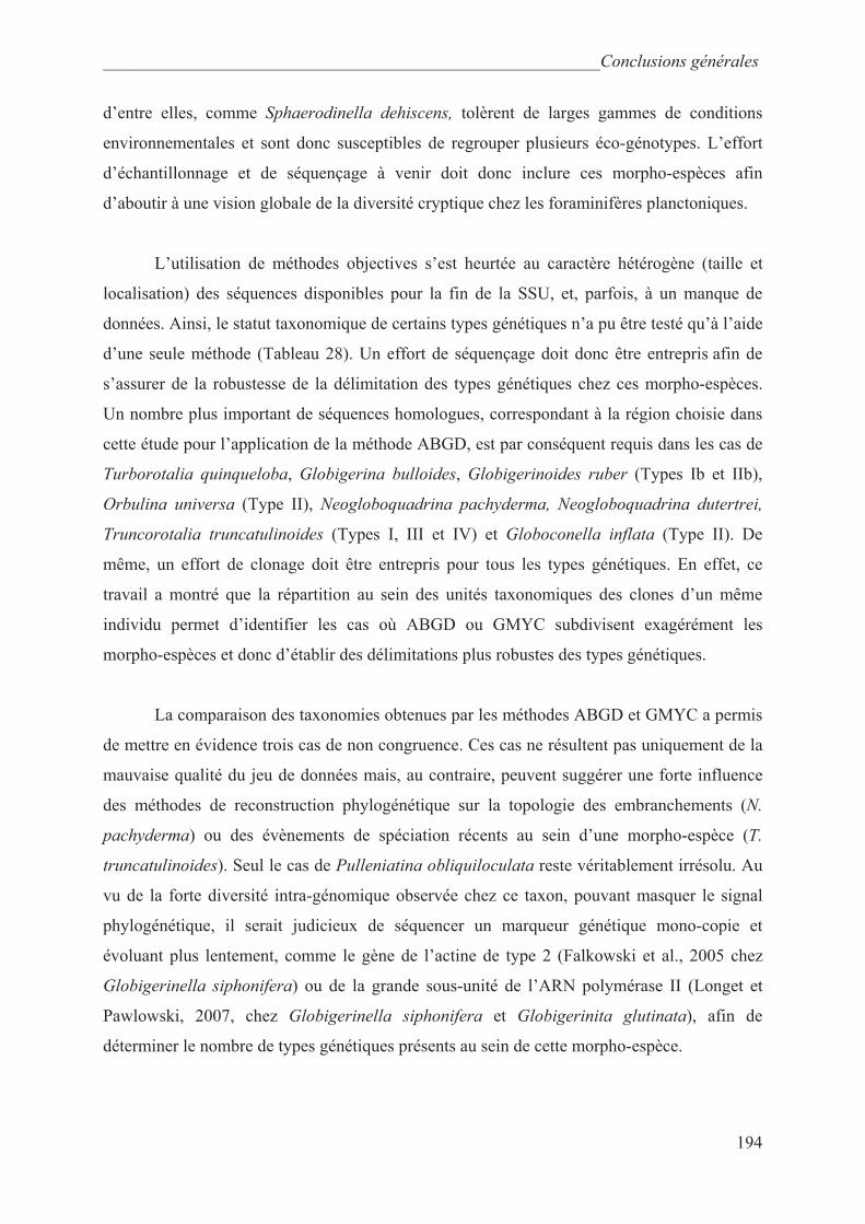
_________________________________________________________Conclusions générales
194
d’entre elles, comme Sphaerodinella dehiscens, tolèrent de larges gammes de conditions
environnementales et sont donc susceptibles de regrouper plusieurs éco-génotypes. L’effort
d’échantillonnage et de séquençage à venir doit donc inclure ces morpho-espèces afin
d’aboutir à une vision globale de la diversité cryptique chez les foraminifères planctoniques.
L’utilisation de méthodes objectives s’est heurtée au caractère hétérogène (taille et
localisation) des séquences disponibles pour la fin de la SSU, et, parfois, à un manque de
données. Ainsi, le statut taxonomique de certains types génétiques n’a pu être testé qu’à l’aide
d’une seule méthode (Tableau 28). Un effort de séquençage doit donc être entrepris afin de
s’assurer de la robustesse de la délimitation des types génétiques chez ces morpho-espèces.
Un nombre plus important de séquences homologues, correspondant à la région choisie dans
cette étude pour l’application de la méthode ABGD, est par conséquent requis dans les cas de
Turborotalia quinqueloba, Globigerina bulloides, Globigerinoides ruber (Types Ib et IIb),
Orbulina universa (Type II), Neogloboquadrina pachyderma, Neogloboquadrina dutertrei,
Truncorotalia truncatulinoides (Types I, III et IV) et Globoconella inflata (Type II). De
même, un effort de clonage doit être entrepris pour tous les types génétiques. En effet, ce
travail a montré que la répartition au sein des unités taxonomiques des clones d’un même
individu permet d’identifier les cas où ABGD ou GMYC subdivisent exagérément les
morpho-espèces et donc d’établir des délimitations plus robustes des types génétiques.
La comparaison des taxonomies obtenues par les méthodes ABGD et GMYC a permis
de mettre en évidence trois cas de non congruence. Ces cas ne résultent pas uniquement de la
mauvaise qualité du jeu de données mais, au contraire, peuvent suggérer une forte influence
des méthodes de reconstruction phylogénétique sur la topologie des embranchements (N.
pachyderma) ou des évènements de spéciation récents au sein d’une morpho-espèce (T.
truncatulinoides). Seul le cas de Pulleniatina obliquiloculata reste véritablement irrésolu. Au
vu de la forte diversité intra-génomique observée chez ce taxon, pouvant masquer le signal
phylogénétique, il serait judicieux de séquencer un marqueur génétique mono-copie et
évoluant plus lentement, comme le gène de l’actine de type 2 (Falkowski et al., 2005 chez
Globigerinella siphonifera) ou de la grande sous-unité de l’ARN polymérase II (Longet et
Pawlowski, 2007, chez Globigerinella siphonifera et Globigerinita glutinata), afin de
déterminer le nombre de types génétiques présents au sein de cette morpho-espèce.
_________________________________________________________Conclusions générales
195
La mise en place d’un référentiel taxonomique chez les foraminifères planctoniques
est un pré-requis pour l’interprétation des jeux de données issus du séquençage
environnemental. Le développement de ces jeux de données sera une opportunité de mieux
connaitre la biogéographie et les variations saisonnières des espèces cryptiques. Ces données
ouvrent donc la voie à une véritable et fructueuse approche intégrative de la taxonomie des
foraminifères planctoniques. De plus, elles devraient permettre de mieux appréhender les
mécanismes à l’origine de la spéciation sympatrique chez ces organismes. Il sera ainsi plus
aisé de mettre en évidence des différences entre les saisons de reproduction et/ou entre les
périodes d’abondances maximales des types génétiques occupant les mêmes régions. De
même, une connaissance plus fine de la biogéographie des types génétiques permettra
d’estimer les flux génétiques entre différentes populations, y compris entre populations
apparemment isolées comme c’est le cas par exemple pour les types génétiques bipolaires.
Une meilleure connaissance des variations saisonnières d’abondance des différents types
génétiques permettra de plus d’établir des relations entre abondances et température des eaux
de surface qui reflètent les abondances annuelles observées dans les sédiments de surface,
utilisés dans la calibration des fonctions de transfert. Enfin, connaitre les variations
d’abondance et la biogéographie des types génétiques permettra de mieux cibler les régions et
les périodes à échantillonner en vue d’analyses morphologiques et/ou géochimiques.
Apport des séquences complètes de la SSU
Jusqu’à présent les rares séquences complètes de la SSU ont été obtenues afin
d’améliorer les reconstructions phylogénétiques entre les principaux clades de foraminifères
(Schweizer et al., 2008 ; Seears, 2011). Cette étude montre que les séquences complètes ont
leur intérêt également pour les phylogénies à l’échelle de la morpho-espèce. Comme ces
séquences restent difficiles à obtenir, elles ne peuvent cependant venir qu’en complément des
séquences partielles de la SSU utilisées classiquement chez les foraminifères planctoniques.
L’exemple de N. pachyderma (Fig. 43) montre que l’obtention de séquences complètes de la
SSU est prometteuse pour résoudre la phylogénie et le découpage taxonomique de cette
morpho-espèce alors que des séquences partielles de la SSU ne permettent pas de répondre à
ces questions de façon satisfaisante. Notamment, les séquences complètes obtenues au cours
de ce travail montrent que le scénario phylogéographique proposé par Darling et al. (2007)
doit être révisé et cette révision entraine une modification de l’interprétation des liens entre
_________________________________________________________Conclusions générales
196
histoires climatique et biologique. Néanmoins, cette étude doit être complétée : les séquences
complètes de la SSU des Types VII, VI et V, plus rarement échantillonnés, sont encore
inconnues. Il faudrait aussi séquencer plusieurs individus par type génétique afin d’estimer la
diversité intra-type génétique et séquencer plusieurs clones d’un même individu afin d’avoir
accès à la variabilité intra-génomique, ce qui est un prérequis pour une délimitation objective
des espèces cryptiques (Partie I, Chapitre 1). Il serait judicieux de réaliser le séquençage
complet de la SSU pour les morpho-espèces dont la délimitation des types génétiques pose
problème (Partie I, chapitre 1). Par exemple, les Types I et II de Truncorotalia
truncatulinoides sont très peu divergents au niveau de la fin de la SSU (de Vargas et al., 2001)
ce qui rend leur statut taxonomique ambigu (Partie I, chapitre 1). L’exemple de N.
pachyderma suggère que le début de la SSU inclut plus de régions variables que la fin (Fig.
43), donc, si cette caractéristique est un trait commun aux foraminifères, le statut
taxonomique des Types I et II de T. truncatulinoides pourrait être résolu à l’aide de séquences
complètes de la SSU.
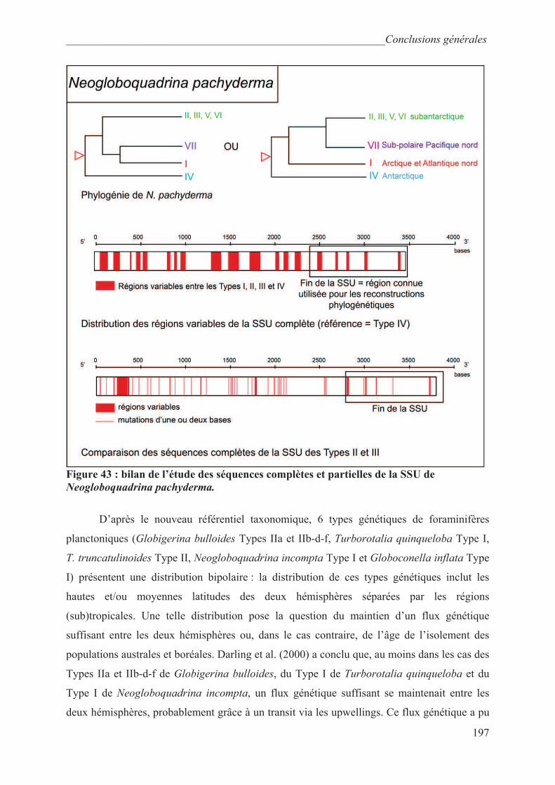
_________________________________________________________Conclusions générales
197
Figure 43 : bilan de l’étude des séquences complètes et partielles de la SSU de
Neogloboquadrina pachyderma.
D’après le nouveau référentiel taxonomique, 6 types génétiques de foraminifères
planctoniques (Globigerina bulloides Types IIa et IIb-d-f, Turborotalia quinqueloba Type I,
T. truncatulinoides Type II, Neogloboquadrina incompta Type I et Globoconella inflata Type
I) présentent une distribution bipolaire : la distribution de ces types génétiques inclut les
hautes et/ou moyennes latitudes des deux hémisphères séparées par les régions
(sub)tropicales. Une telle distribution pose la question du maintien d’un flux génétique
suffisant entre les deux hémisphères ou, dans le cas contraire, de l’âge de l’isolement des
populations australes et boréales. Darling et al. (2000) a conclu que, au moins dans les cas des
Types IIa et IIb-d-f de Globigerina bulloides, du Type I de Turborotalia quinqueloba et du
Type I de Neogloboquadrina incompta, un flux génétique suffisant se maintenait entre les
deux hémisphères, probablement grâce à un transit via les upwellings. Ce flux génétique a pu
_________________________________________________________Conclusions générales
198
se maintenir au cours du temps et même s’intensifier lors des périodes glaciaires (Darling et
al., 2000). La comparaison des séquences complètes obtenues pour le type génétique bipolaire
(Type I) de Neogloboquadrina incompta au cours de cette étude (hémisphère sud) et par
Seears (2011, hémisphère nord) vient tempérer, voire remettre en cause, cette hypothèse. En
effet, ces séquences présentent des différences jusque-là insoupçonnées pouvant résulter
d’une diminution du flux génétique trans-équatorial. Ces différences doivent toutefois être
confirmées par l’obtention d’un nombre plus important de séquences. Il serait donc pertinent
de réaliser le séquençage complet de la SSU pour les types génétiques bipolaires afin de
déterminer s’il existe de véritables haplotypes bipolaires.
Taxonomies moléculaire et morphologique : les cas exceptionnels de
Globigerinoides sacculifer et Neogloboquadrina pachyderma
La diversité cryptique semble être la règle dans le domaine pélagique (Knowlton,
1993) et les foraminifères ne font pas exception. En effet, jusqu’à présent, chacune des
morpho-espèces dont l’échantillonnage en vue d’analyses génétiques a été particulièrement
poussé, s’est révélée être le regroupement de plusieurs types génétiques (Darling et al., 2008).
Le premier chapitre de cette thèse a conclu qu’une partie de ces types génétiques
correspondait très certainement à des espèces différentes. Globigerinoides sacculifer fait
exception à cette règle puisque cette morpho-espèce, pourtant ancienne (~19 Ma, Kennett et
Srinivasan, 1983 ; Berggren et al., 1995), présente une très faible diversité génétique
correspondant à de la diversité intra-spécifique (Partie I, chapitre 1 et Partie II, chapitre 1).
Néanmoins, nous avons montré dans ce travail qu’il reste encore possible de mettre en
évidence une absence de diversité cryptique parmi les espèces moins abondantes encore peu
étudiées. Avec l’augmentation des données disponibles, de plus en plus de cas d’absence de
diversité cryptique, chez des taxons allant du requin pèlerin (Hoelzel et al., 2006) aux
dinoflagellés (Logares et al., 2007 ; Montresor et al., 2003), montrent que si la diversité
cryptique est courante chez les organismes pélagiques, elle n’est cependant pas systématique.
Le cas de G. sacculifer pose la question de l’âge de l’espèce biologique : s’agit-il bien
de la même espèce depuis 19 Ma ou bien d’autres espèces de G. sacculifer aujourd’hui
disparues, de morphologie similaire, l’ont-t-elle précédée ? Et surtout, si ces espèces ont
effectivement existé, avaient-elles les mêmes affinités écologiques que l’espèce actuelle ? Si
ce n’est pas le cas, alors l’utilisation de G. sacculifer comme proxy paléoclimatique dans les
séries les plus anciennes peut être remise en cause. De façon plus générale, le problème de
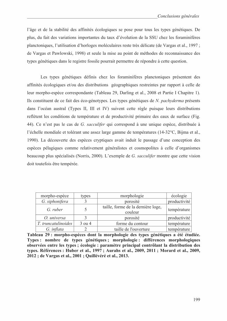
_________________________________________________________Conclusions générales
199
l’âge et de la stabilité des affinités écologiques se pose pour tous les types génétiques. De
plus, du fait des variations importantes du taux d’évolution de la SSU chez les foraminifères
planctoniques, l’utilisation d’horloges moléculaires reste très délicate (de Vargas et al., 1997 ;
de Vargas et Pawlowski, 1998) et seule la mise au point de méthodes de reconnaissance des
types génétiques dans le registre fossile pourrait permettre de répondre à cette question.
Les types génétiques définis chez les foraminifères planctoniques présentent des
affinités écologiques et/ou des distributions géographiques restreintes par rapport à celle de
leur morpho-espèce correspondante (Tableau 29, Darling et al., 2008 et Partie I Chapitre 1).
Ils constituent de ce fait des éco-génotypes. Les types génétiques de N. pachyderma présents
dans l’océan austral (Types II, III et IV) suivent cette règle puisque leurs distributions
reflètent les conditions de température et de productivité primaire des eaux de surface (Fig.
44). Ce n’est pas le cas de G. sacculifer qui correspond à une unique espèce, distribuée à
l’échelle mondiale et tolérant une assez large gamme de températures (14-32°C, Bijma et al.,
1990). La découverte des espèces cryptiques avait induit le passage d’une conception des
espèces pélagiques comme relativement généralistes et cosmopolites à celle d’organismes
beaucoup plus spécialisés (Norris, 2000). L’exemple de G. sacculifer montre que cette vision
doit toutefois être tempérée.
morpho-espèce types morphologie écologie
G. siphonifera 3 porosité productivité
G. ruber 5 taille, forme de la dernière loge,
couleur température
O. universa 3 porosité productivité
T. truncatulinoides 3 ou 4 forme du contour température
G. inflata 2 taille de l'ouverture température
Tableau 29 : morpho-espèces dont la morphologie des types génétiques a été étudiée.
Types : nombre de types génétiques ; morphologie : différences morphologiques
observées entre les types ; écologie : paramètre principal contrôlant la distribution des
types. Références : Huber et al., 1997 ; Aurahs et al., 2009, 2011 ; Morard et al., 2009,
2012 ; de Vargas et al., 2001 ; Quillévéré et al., 2013.
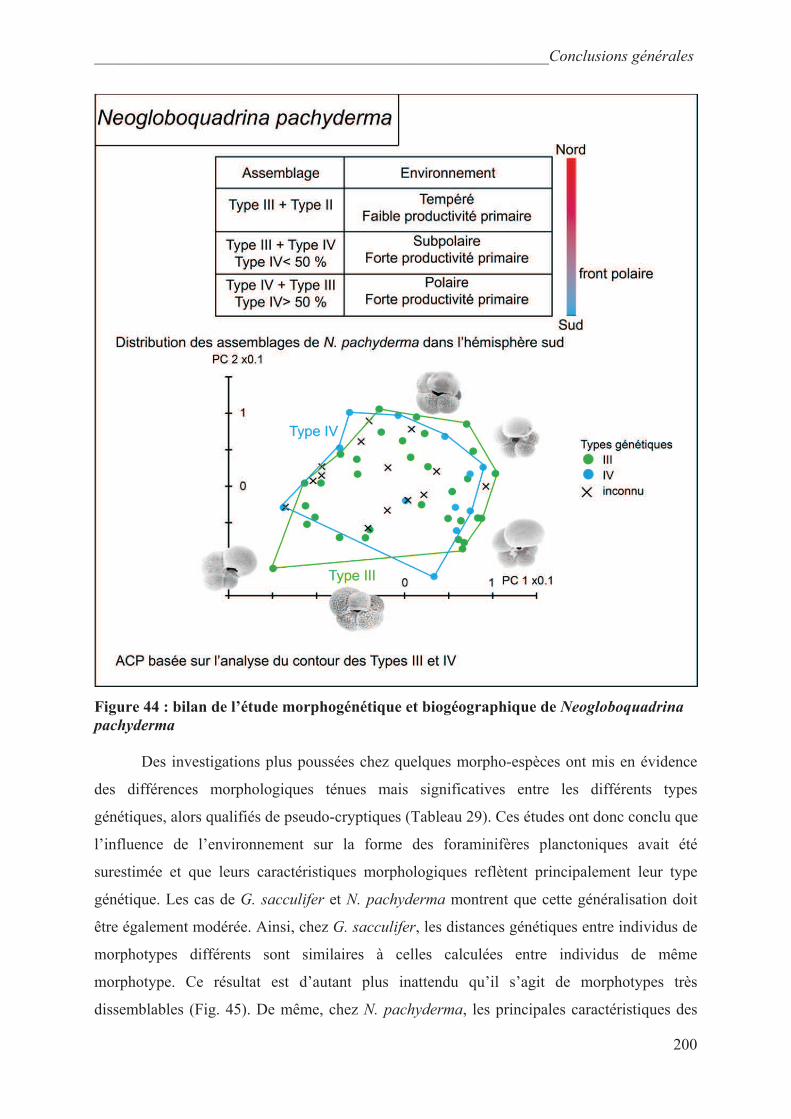
_________________________________________________________Conclusions générales
200
Figure 44 : bilan de l’étude morphogénétique et biogéographique de Neogloboquadrina
pachyderma
Des investigations plus poussées chez quelques morpho-espèces ont mis en évidence
des différences morphologiques ténues mais significatives entre les différents types
génétiques, alors qualifiés de pseudo-cryptiques (Tableau 29). Ces études ont donc conclu que
l’influence de l’environnement sur la forme des foraminifères planctoniques avait été
surestimée et que leurs caractéristiques morphologiques reflètent principalement leur type
génétique. Les cas de G. sacculifer et N. pachyderma montrent que cette généralisation doit
être également modérée. Ainsi, chez G. sacculifer, les distances génétiques entre individus de
morphotypes différents sont similaires à celles calculées entre individus de même
morphotype. Ce résultat est d’autant plus inattendu qu’il s’agit de morphotypes très
dissemblables (Fig. 45). De même, chez N. pachyderma, les principales caractéristiques des
_________________________________________________________Conclusions générales
201
coquilles (nombre de loges sur le dernier tour, taille de la dernière loge) ainsi que leur forme
(Fig. 44) ne sont pas corrélables aux types génétiques mais sont bien d’origine éco-
phénotypique.
La découverte des espèces pseudo-cryptiques suggère une possible réconciliation entre
morpho-taxonomie et taxonomie moléculaire (Huber et al., 1997 ; Aurahs et al., 2009, 2011 ;
Morard et al., 2009, 2011 ; de Vargas et al., 2001 ; Quillévéré et al., 2013). Cette
réconciliation est possible chez G. sacculifer à condition d’abolir la distinction entre les divers
morphotypes et notamment la distinction « avec sac » et « sans sac » encore utilisée (par
exemple, Prell, 1999). Par contre cette réconciliation reste impossible pour les types
génétiques austraux de N. pachyderma. Or, cette morpho-espèce représente la presque totalité
des assemblages de hautes latitudes australes et boréales sont largement dominés chacun par
un unique type génétique de N. pachyderma (Type I dans l’Atlantique nord, Type VII dans le
Pacifique nord, Darling et al., 2007). Par conséquent, l’intégration des espèces cryptiques des
foraminifères planctoniques dans les fonctions de transfert en vue d’améliorer la précision des
reconstructions paléocéanographiques est compromise pour ces environnements.

_________________________________________________________Conclusions générales
202
Figure 45 : bilan de l’étude morphogénétique et biogéographique de Globigerinoides
sacculifer
Les liens entre diversité génétique et morphologique chez les foraminifères semblent
au final variables d’une morpho-espèce à l’autre et il est difficile de prévoir quel critère
morphologique peut être mis en relation avec la diversité génétique d’un taxon. Ainsi, chez
G. sacculifer et N. pachyderma, l’aspect de la dernière loge n’a pas de valeur taxonomique
(Partie II) alors que ce même critère permet de différentier les Types I et II de
_________________________________________________________Conclusions générales
203
Globogerinoides ruber. La difficulté de réconcilier taxonomies morphologique et moléculaire
est attendue car les taux d’évolution de la SSU et les taux d’évolution morphologique ne sont
pas directement liés. Chez les foraminifères, il est probable que les différences entre espèces
cryptiques soient d’ordre plus métabolique que morphologique: différences de régime
alimentaire et/ou différences dans les modes de reproduction par exemple. Une trace de ces
différences métaboliques peut toutefois être conservée après la mort du foraminifère car un
métabolisme différent peut se traduire par un fractionnement isotopique et élémentaire
différent, l’«effet vital », qui peut atteindre, par exemple, 1.5‰ pour le 18
O chez les
foraminifères planctoniques (Katz et al., 2010). L’analyse géochimique des coquilles des
types génétiques de N. pachyderma pourrait donc permettre :
1) d’établir des équations de paléotempérature calibrées à l’échelle de l’espèce
cryptique. Ces équations pourraient être alors utilisées dans le registre fossile pour les régions
n’abritant qu’une seule espèce cryptique (Atlantique nord, Pacifique nord et environnements
polaires extrêmes de l’Antarctique).
2) de différentier des espèces cryptiques au sein d’un assemblage et donc de les inclure
dans la calibration des fonctions de transfert.
Néanmoins, la mise en évidence d’effets vitaux différents implique de pouvoir s’affranchir
des variations issues de l’environnement, donc de travailler soit à partir de pools d’individus
de même type génétique, de même stade ontogénétique et de même provenance, soit de
travailler à l’échelle de l’individu. Une analyse individuelle a été tentée chez les Types II, III
et IV de N. pachyderma au cours de ce travail, mais la quantité de CaCO3 présente dans ces
coquilles, n’ayant pas atteint le stade gamétogénétique, s’est révélée trop faible pour pouvoir
être détectée par le spectromètre de masse. Une utilisation de routine des signatures
isotopiques des types génétiques de N. pachyderma n’est donc pas encore envisageable.
Pour conclure, les cas de G. sacculifer et N. pachyderma montrent que spéciation,
diversification morphologique et exigences écologiques ne suivent pas de règle chez les
foraminifères planctoniques contrairement à ce que suggéraient les études précédentes.
L’interprétation des jeux de données issus du séquençage environnemental, rendue possible
par la mise au point d’un référentiel taxonomique adéquat, permettra très probablement de
mettre au jour d’autres exceptions, et finalement de mieux comprendre la dynamique des
écosystèmes pélagiques.
__________________________________________________________________Références
204
REFERENCES
Adl, S., Simpson, A., Farmer, M., Andersen, R., Anderson, O., Barta, J., Bowser, S.,
Brugerolle, G., Fensome, R., Fredericq, S., James, T., Karpov, S., Kugrens, P., Krug, J.,
Lane, C., Lewis, L., Lodge, J., Lynn, D., Mann, D., McCourt, R., Mendoza, L.,
Moestrup, O., Mozley-Standridge, S., Nerad, T., Shearer, C., Smirnov, A., Spiegel, F.
and Taylor, M., 2005. The new higher level classification of eukaryotes with emphasis
on the taxonomy of protists. Journal of Eukaryotic Microbiology, 52: 399-451.
Anand, P. and Elderfield, H., 2003. Calibration of Mg/Ca thermometry in planktonic
foraminifera from a sediment trap time series. Paleoceanography, 18: 1050-1064.
Akaike, H., 1974. A new look at the statistical model identification. Institute of Electrical and
Electronics Engineers Transactions on Automatic Control, 19: 716-723.
Andersson, J.O., 2005. Lateral gene transfert in eucaryotes. Cellular and Molecular Life
Science, 62: 1182-1197.
André, A., Weiner, A., Quillévéré, F., Aurahs, R., Morard, R., Douady, C., de Garidel-
Thoron, T., Escarguel, G., de Vargas, C. and Kucera, M., 2013. The cryptic and the
apparent reversed: lack of genetic differentiation within the morphologically diverse
plexus of the planktonic foraminifer Globigerinoides sacculifer. Paleobiology, 39: 21-
39.
André, A., Quillévéré, F., Morard, R., de Vargas, C., Ujiié, Y., and Douady, C., in prep. A.
SSU rDNA divergence in planktonic foraminifera: molecular taxonomy and
biogeographic implications.
André, A., Quillévéré, F., Escarguel, G., Michel, E. and Douady, C., in prep. B. A case of true
cryptic species within planktonic foraminifera: eco-phenotypic morphological variations
of Southern Ocean Neogloboquadrina pachyderma genetic types.
Aurahs, R., Göker, M., Grimm, G., Hemleben, V., Hemleben, C., Schiebel, R. and Kucera,
M., 2009. Using the multiple analysis approach to reconstruct phylogenetic
relationships among planktonic foraminifera from highly divergent and length-
polymorphic SSU rDNA sequences. Bioinformatics and Biology Insights, 3: 155-177.
Aurahs, R., Grimm, G., Hemleben, V., Hemleben, C. and Kucera, M., 2009. Geographical
distribution of cryptic genetic types in the planktonic foraminifer Globigerinoides
ruber. Molecular Ecology, 18: 1692-1706.
Aurahs, R., Treis, Y., Darling, K. and Kucera, M., 2011. A revised taxonomic and
phylogenetic concept for the planktonic foraminifer species Globigerinoides ruber
based on molecular and morphometric evidence. Marine Micropaleontology, 79: 1-14.
Aze, T., Ezard, T., Purvis, T., Coxall, H., Stewart, D., Wade, B. and Pearson, P., 2011. A
phylogeny of Cenozoic macroperforate planktonic foraminifera from fossil data.
Biological Reviews, 86: 900-927.
__________________________________________________________________Références
205
Bachy, C., Dolan, J., Lopez-Garcia, P., Deschamps, P. and Moreira, D., 2013. Accuracy of
protist diversity assessments: morphology compared with cloning and direct
pyrosequencing of 18S rDNA genes and ITS regions using the conspicuous tintinnid
ciliates as a case study. The International Society for Microbial Ecology Journal, 00: 1-
12.
Bandelt, H.J., Forster, P. and Röhl, A., 1999. Median Joining networks for inferring
intraspecific phylogenies. Molecular Biology and Evolution, 16: 37–48
Bandy, O.L., 1972. Origin and development of Globorotalia (Turborotalia) pachyderma
(Ehrenberg). Micropaleontology, 18: 294-318.
Banner, F.T. and Blow, W.H., 1960. Some primary types of species belonging to the
superfamily Globigerinaceae. Contributions from the Cushman Foundation for
Foraminiferal Research, 11: 1–45.
Bard, E. and Rickaby, R.E.M., 2009. Migration of the subtropical front as a modulator of
glacial climate. Nature, 560: 380–384.
Barker, S., Cacho, I., Benway, H. and Takachikawa, K., 2005. Planktonic foraminiferal
Mg/Ca as a proxy for past oceanic temperatures: a methodological overview and data
compilation for the Last Glacial Maximum. Quaternary Science Reviews, 24: 821-834.
Barrows, T.T. and Juggins, S., 2005. Sea-surface temperatures around the Australian margin
and Indian Ocean during the Last Glacial Maximum. Quaternary Science Review, 24:
1017–1047.
Bartoli, G., Sarnthien, M., Weinelt, M., Erlenkeuser, H., Garbe-Schonberg, D. and Lea, D.,
2005. Final closure of Panama and the onset of northern hemisphere glaciation. Earth
and Planetary Science letters, 237: 33-44.
Bé, A.W., 1959. Ecology of recent planktonic foraminifera: Part I –Areal distribution in the
western North Atlantic. Micropaleontology, 5: 77-100.
Bé, A.W., 1960. Some observations on arctic planktonic foraminifera. Contributions of the
Cushman Foundation for Foraminiferal Research, 11: 64-68.
Bé, A.W. and Hemleben, C., 1970. Calcification in a living planktonic foraminifer,
Globigerinoides sacculifer (Brady). Neue Jahrbuch für Geologie und Paläontologie
abhandlungen, 134: 221-234.
Bé, A.W.H. and Tolderlund, D.S., 1971. Distribution and ecology of planktonic foraminifera.
The micropaleontology of oceans, Cambridge University Press, London.
Bé, A.W., 1980. Gametogenetic calcification in a spinose planktonic foraminifer,
Globigerinoides sacculifer (Brady). Marine Micropaleontology, 5: 283–310.
Bé, A.W., Anderson, O.R., Faber, W.W. and Caron, D.A., 1983. Sequence of morphological
and cytoplasmic changes during gametogenesis in the planktonic foraminifer
Globigerinoides sacculifer (Brady). Micropaleontology, 29: 319–325.
Beal, L.M., de Ruijter, W.P., Biastoch, A., Zahn, R. and SCOR/WCRP/IAPSO Working
Group 136, 2011. On the role of the Agulhas system in ocean circulation and climate.
Nature, 472: 429–436.
__________________________________________________________________Références
206
Becquey, S. and Gersonde, R., 2003. A 0.55-Ma paleotemperature record from the
subantarctic zone: implications for Antarctic Circumpolar Current development.
Paleoceanography, 18: 1014-1028.
Begon, M., Harper, J.L. and Townsend, J.R., 1986. Ecology : individuals, populations and
communities. Blackwell Scientific Publications, Oxford.
Bergami, C., Capotondi, L., Langone, L., Giglio, F. and Ravaioli, M., 2009. Distribution of
living planktonic foraminifera in the Ross Sea and the Pacific sector of the Southern
Ocean (Antarctica). Marine Micropaleontology, 73: 37-48.
Berger, W.H., 1969. Planktonic foraminifera: basic morphology and ecologic implications.
Journal of paleontology, 43: 1369-1383.
Berggren, W.A., Kent, D.V., Swisher, C.C. and Aubry, M-P., 1995. A revised Cenozoic
geochronology and chronostratigraphy. Geochronology, time scales and global
stratigraphic correlation, SEPM (Society for Sedimentary Geology), Tulsa (Oklahoma).
Bickford, D., Lohman, D.J., Sodhi, N.S., Ng, P.K.L., Meier, R., Winker, K., Ingram, K.K. and
Das, I., 2007. Cryptic species as a window on diversity and conservation. Trends in
Ecology and Evolution, 22:148–155.
Bijma, J., Erez, J. and Hemleben, C., 1990. Lunar and semi-lunar reproductive cycles in some
spinose planktonic foraminifers. Journal of Foraminiferal Research, 20:117–127.
Bijma, J., Faber, W.W. and Hemleben, C., 1990. Temperature and salinity limits for growth
and survival of some planktonic foraminifers in laboratory cultures. Journal of
Foraminiferal Research, 20: 95-116.
Bijma, J., Hemleben, C., Oberhänsli, H. and Spindler, M., 1992. The effects of increased
water fertility on tropical spinose planktonic foraminifers in laboratory cultures. Journal
of Foraminiferal Research, 22:242–256.
Bijma, J., Hemleben, C., Huber, B.T., Erlenkeuser, H. and Kroon, D., 1998. Experimental
determination of the ontogenetic stable isotope variability in two morphotypes of
Globigerinella siphonifera (d'Orbigny). Marine Micropaleontology, 35: 141-160.
Bolli, H. and Saunders, J., 1985. Oligocene to Holocene low latitude planktic foraminifera.
Plankton stratigraphy. Cambridge University Press, Cambridge.
Boltovskoy, D., Correa, N. and Boltovskoy, A., 2003. Marine zooplanktonic diversity: a view
from the South Atlantic. Oceanologica Acta, 25: 271-278.
Brady, H.B., 1877. Supplementary note on the foraminifera of the chalk (?) of the New
Britain group. Geological Magazine London, 4: 534–536.
Briggs, J.C., 1994. Species diversity: land and sea compared. Systematic Biology, 43: 130-
135.
Broecker, W.S., 1982. Ocean chemistry during glacial time. Geochimica et Cosmochimica
Acta, 46: 1689-1705.
__________________________________________________________________Références
207
Budillon, F., Lirer, F., Iorio, M., Macri, P., Sagnotti, L., Vallefuoco, M., Ferraro, L.,
Garziglia, S., Innangi, S., Sahabi, M. and Tonielli, R., 2009. Integrated stratigraphic
reconstruction for the last 80 kyr in deep sector of the Sardinia Channel (Western
Mediterranean). Deep Sea Research Part II, Topical Studies in Oceanography, 56: 725–
737.
Caron, D.A. and Bé, A.W.H., 1984. Predicted and observed feeding rates of the spinose
planktonic foraminifer Globigerinoides sacculifer. Bulletin of Marine Science, 35: 1-10.
Carter, L., McCave, I.N., Williams, M.J.M., Fabio, F. and Martin, S., 2008. Chapter 4
circulation and water masses of the Southern Ocean: a review. Developments in Earth
and Environmental Sciences, Elsevier, Amsterdam.
Castresana, J., 2000. Selection of conserved blocks from multiple alignments for their use in
phylogenetic analysis. Molecular Biology and Evolution, 17: 540-552.
Cavalier-Smith, T. and Chao, E.E.Y., 2003. Phylogeny and classification of phylum Cercozoa
(Protozoa). Protist, 154: 341-358.
Clarke, K.R., 1993. Non-parametric multivariate analysis of changes in community structure.
Australian Journal of Ecology, 18: 117–143.
Cifelli, R., 1961. Globigerina incompta, a new species of pelagic foraminiera from the North
Atlantic Ocean. Contributions of the Cushman Foundation for Foraminiferal Research,
12: 83-86.
CLIMAP, 1981. Seasonnal reconstructions of the Earth's surface at the last glacial maximum.
Geological Society of Americain Map and Chart Series, MC-36.
Coleman, A.W., 2003. ITS2 is a double-edged tool for eukaryote evolutionary comparisons.
Trends in Genetics, 19: 370-375.
Coleman, A.W., 2009. Is there a molecular key to the level of “biological species” in
eukaryotes? A DNA guide. Molecular Phylogenetics and Evolution, 50: 197-203.
Collen, J.D. and Vella, P., 1973. Pliocene planktonic foraminifera, southern North Island,
New Zealand. The Journal of Foraminiferal Research, 3: 13-29.
Coyne, J. and Orr, H., 2004. Speciation chapter 1. Speciation, Sinauser, Sunderland
(Massachusetts).
Darling, K.F., Kroon, D., Wade, C.M. and Leigh Brown, A.J., 1996. Molecular phylogeny of
the planktic foraminifera. Journal of Foraminiferal Research, 26: 324-330.
Darling, K.F., Wade, C.M., Kroon, D. and Brown, A.J., 1997. Planktic foraminiferal
molecular evolution and their polyphyletic origins from benthic taxa. Marine
Micropaleontology, 30: 251–266.
Darling, K.F., Wade, C.M., Kroon, D., Brown, A.J.L. and Bijma, J., 1999. The diversity and
distribution of modern planktic foraminiferal small subunit ribosomal RNA genotypes
and their potential as tracers of present and past circulation. Paleoceanography, 14: 3-
12.

__________________________________________________________________Références
208
Darling, K.F., Wade, C.M., Stewart, I.A., Kroon, D., Dingle R. and Brown, A.J., 2000.
Molecular evidence for genetic mixing of Arctic and Antarctic subpolar populations of
planktonic foraminifers. Nature, 405: 43-47.
Darling, K.F., Kucera, M., Wade, C.M., Langen, P.V. and Pak, D., 2003. Seasonal
distribution of genetic types of planktonic foraminifer morphospecies in the Santa
Barbara Channel and its paleoceanographic implications. Paleoceanography, 18:
1032¬1042.
Darling, K.F., Kucera, M., Pudsey, C.J. and Wade, C.M., 2004. Molecular evidence links
cryptic diversification in polar planktonic protists to Quaternary climate dynamics.
Proceedings of the National Academy of Sciences of the United States of America, 101:
7657-7662.
Darling, K.F., Kucera, M., Kroon, D. and Wade, C.M., 2006. A resolution for the coiling
direction paradox in Neogloboquadrina pachyderma. Paleoceanography, 21: 1-14.
Darling, K.F., Kucera, M. and Wade, C.M., 2007. Global molecular phylogeography reveals
persistent arctic circumpolar isolation in a marine planktonic protist. Proceedings of the
National Academy of Sciences of the United States of America, 104: 5002-5007.
Darling, K.F. and Wade, C.M., 2008. The genetic diversity of planktic foraminifera and the
global distribution of ribosomal RNA genotypes. Marine Micropaleontology, 67:
216¬238.
Dayrat, B., 2005. Towards integrative taxonomy. Biological Journal of the Linnean Society,
85: 407-415.
De Aguiar, M.A.M., Baranger, M., Baptestini, E.M., Kaufman, L. and Bar-Yam, Y., 2009.
Global patterns of speciation and diversity. Nature 460: 384-387.
de Queiroz, K., 2005. Ernst Mayr and the modern concept of species. Proceedings of the
National Academy of Sciences of the United States of America, 102: 6600-6607.
de Queiroz, K., 2007. Species concepts and species delimitation. Systematic Biology, 56:
879-886.
de Vargas, C., Zaninetti, L., Hilbrecht, H. and Pawlowski, J., 1997. Phylogeny and rates of
molecular evolution of planktonic foraminifera: SSU rDNA sequences compared to the
fossil record. Journal of Molecular Evolution, 45: 285-294.
de Vargas, C., and Pawlowski, J., 1998. Molecular versus taxonomic rates of evolution in
planktonic foraminifera. Molecular Phylogenetics and Evolution, 9:463–469.
de Vargas, C., Norris, R.D., Zaninetti, L., Gibb, S.W. and Pawlowski, J., 1999. Molecular
evidence of cryptic speciation in planktonic foraminifers and their relation to oceanic
provinces. Proceedings of the National Academy of Sciences of the United States of
America, 96: 2864-2868.
de Vargas, C., Renaud, S., Hilbrecht, H. and Pawlowski, J., 2001. Pleistocene adaptive
radiation in Globorotalia truncatulinoides: genetic, morphologic, and environmental
evidence. Paleobiology, 27: 104-125.
__________________________________________________________________Références
209
de Vargas, C., Bonzon, M., Rees, N.W., Pawlowski, J. and Zaninetti, L., 2002. A molecular
approach to biodiversity and biogeography in the planktonic foraminifer Globigerinella
siphonifera (d'Orbigny). Marine Micropaleontology, 45: 101-116.
de Vernal., A. and Hillaire-Marcel, C., 2006. Provincialism in trends and high frequency
change in the northwest North Atlantic during the Holocene. Global Planetary Change,
54: 263-290.
Dieckmann, G.S., Spindler, M., Mange, M.A., Ackley, S.F. and Eicken, H., 1991. Antarctic
sea ice: a habitat for the foraminifer Neogloboquadrina pachyderma. Journal of
Foraminiferal Research, 21: 183-189.
d’Orbigny, A., 1846. Foraminifères fossiles du bassin tertiaire de Vienne (Autriche). Gide et
Comp, Paris.
Drummond, A.J., Suchard, M.A., Xie, D. and Rambaut, A., 2012. Bayesian phylogenetics
with BEAUti and the BEAST 1.7. Molecular Biology and Evolution, 8:1969-1973.
Edgar, R.C., 2004. MUSCLE: multiple sequence alignment with high accuracy and high
throughput. Nucleic Acids Research, 32: 1792-1797.
Elmer, K., Davila, J. and Lougheed, S., 2007. Cryptic diversity and deep divergence in an
upper Amazonian leaflitter frog, Eleutherodactylus ockendeni. BioMed Central
Evolutionary Biology, 7: 247.
Emery, W.J. and Meincke, J., 1986. Global water masses: summary and review. Oceanologica
Acta, 9: 383-391.
Erez, J. and Luz, B., 1983. Experimental paleotemperature equation for planktonic
foraminifera. Geochimica et Cosmochimica Acta, 47: 1025-1031.
Ericson, D.B., 1959. Coiling direction of Globigerina pachyderma as a climatic index.
Science, 130: 219–220.
Ertan, K.T., Hemleben, V. and Hemleben, C., 2004. Molecular evolution of some selected
benthic foraminifera as inferred from sequences of the small subunit ribosomal DNA.
Marine Micropaleontology, 53: 367-388.
Eynaud, F., Cronin, T.M., Smith, S.A., Zaragosi, S., Mavel, J., Mary, Y, Mas, V. and Pujol,
C., 2009. Morphological variability of the planktonic foraminifer Neogloboquadrina
pachyderma from ACEX cores: implications for the Late Pleistocene circulation of the
Arctic Ocean. Micropaleontology, 55: 101-116.
Ezard, T., Fujisawa, T. and Barraclough, T., 2009. Splits: SPecies' LImits by Threshold
Statistics. R package version 1.0-11/r29.
Fairbanks, R.G. and Weibe, P., 1980. Foraminifera and chlorophyll maximum: vertical
distribution, seasonal succession, and paleoceanographic significance. Science, 209:
1524-1526.
Fenchel, T., 2005. Cosmopolitan microbes and their cryptic species. Aquatic Microbial
Ecology, 41: 49-54.
__________________________________________________________________Références
210
Finlay, B.J., 2002. Global dispersal of free-living microbial eukaryote species. Science, 296:
1061-1063.
Flakowski, J., Bolivar, I., Fahrni, J. and Pawlowski, J., 2005. Actin phylogeny of
foraminifera. Journal of Foraminiferal Research, 35: 93-102.
Flores, J.-A., Gersonde, R. and Sierro, F., 1999. Pleistocene fluctuations in the Agulhas
Current Retroflection based on the calcareous plankton record. Marine
Micropaleontology, 37:1–22.
Fontaneto, D., Herniou, E.A., Boschetti, C., Caprioli, M., Melone, G., Ricci, C. and
Barraclough, T.G., 2007. Independently evolving species in asexual Bdelloid rotifers.
Public Library of Science Biology, 5: e87.
Foote, M., 1989. Perimeter-based Fourier analysis: A new morphometric method applied to
the trilobite cranidium. Journal of Paleontology, 63: 880-885.
Gascuel, O., 1997. BIONJ: an improved version of the NJ algorithm based on a simple model
of sequence data. Molecular Biology and Evolution, 14: 685-695.
Gast, R.J. and Caron, D.A., 1996. Molecular phylogeny of symbiotic dinoflagellates from
planktonic foraminifera and radiolaria. Molecular Biology and Evolution, 13:
1192¬1197.
Görker, M., Grimm, G.W., Auch, A.F., Aurahs, R. and Kucera, M., 2010. A clustering
optimization strategy for molecular taxonomy applied to planktonic foraminifera SSU
rDNA. Evolutionary Bioinformatics, 6: 97-112.
Grimm, G.W., Stogerer, K., Ertan, K., Kitazato, H., Kucera, M., Hemleben, V. and
Hemleben, C., 2007. Diversity of rDNA in Chilostomella: molecular differentiation
patterns and putative hermit types. Marine Micropaleontology, 62: 75-90.
Groeneveld, J., Steph, S., Tiedemann, R., Garbe-Schonberg, D., Nurnberg, D. and Sturm, A.,
2006. Pliocene mixed layer oceanography for site 1241 using combined Mg/Ca and
18O analyses of Globigerinoides sacculifer. Proceedings of the Ocean Drilling
Program, Scientific Results, 202:1–27.
Gouy, M., Guindon, S.P. and Gascuel, O., 2010. SeaView Version 4: a multiplatform
graphical user interface for sequence alignment and phylogenetic tree building.
Molecular Biology and Evolution, 27: 221-224.
Guindon, S. and Gascuel, O., 2003. A simple, fast, and accurate algorithm to estimate large
phylogenies by maximum likelihood. Systematic Biology, 52:696-704.
Hammer, Ø., Harper, D.A.T. and Ryan, P.D., 2001. PAST: Paleontological statistics software
package for education and data analysis. Palaeontologia Electronica, 4: 9.
Hart, M.B., Hylton, M.D., Oxford, M.J., Hudson, W. and Smart, C.W., 2003. The search for
the origin of the planktic Foraminifera. Journal of the Geological Society, 160: 341-343.
Healy-Williams, N., 1984. Quantitative image analysis: application to planktonic
foraminiferal paleoecology and evolution. Geobios, 17: 425-432.
__________________________________________________________________Références
211
Hecht, A.D. and Savin, S.M., 1970. Oxygen-18 studies on recent planktonic foraminifera:
comparaison of phenotypes and test parts. Science, 170: 69.
Hecht, A.D., 1974. Intraspecific variation in recent populations of Globigerinoides ruber and
Globigerinoides trilobus and their application to paleoenvironmental analysis. Journal
of Paleontology, 48:1217–1234.
Hecht, A.D., 1976. An ecologic model for test size variation in recent planktonic
foraminifera: applications to the fossil record. Journal of Foraminiferal Research, 6:
295-311.
Hemleben, C., Spindler, M., Breitinger, I. and Ott., R., 1987. Morphological and
physiological responses of Globigerinoides sacculifer (Brady) under varying laboratory
conditions. Marine Micropaleontology, 12: 305–324.
Hemleben, C., Spindler, M. and Anderson, O.R., 1989. Modern Planktonic Foraminifera.
Springer, New York.
Hess, W.R., 2004. Genome analysis of marine photosynthetic microbes and their global role.
Current Opinion in Biotechnology, 15: 191-198.
Hilbrecht, H., 1997. Morphologic gradation and ecology in Neogloboquadrina pachyderma
and N. dutertrei (planktic foraminifera) from core top sediments. Marine
Micropaleontology, 31: 31-43.
Hilbrecht, H., 1996. Extant planktic foraminifera and the physical environment in the Atlantic
and Indian Oceans. Technischen Hochschule und der Universität Zürich, Neue Folge,
Zürich.
Hoef-Emden, K., 2012. Pitfalls of establishing DNA barcoding systems in protists: the
Chrysophyceae as a test case. Public Library of Science One, 7: e45632.
Hoelzel, A., Mahmood, S., Magnussen, J. and Francis, M.P., 2006. Low worldwide genetic
diversity in the basking shark (Cetorhinus maximus). Biology Letters, 2: 639-642.
Holzmann, M. and Pawlowski, J., 1996. Preservation of foraminifera for DNA extraction and
PCR amplification. The Journal of Foraminiferal Research, 26: 264-267.
Hofker, J., 1959. On the splitting of Globigerina. Contributions from the Cushman
Foundation for Foraminiferal Research, 10:1–9.
Huber, B.T. and Leckie, R.M., 2011. Planktonic foraminiferal species trunover across deep-
sea Aptian/Albian boundary sections. Journal of Foraminiferal Research, 41: 53-95.
Huber, B.T., Bijma, J. and Darling, K.F., 1997. Cryptic speciation in the living planktonic
foraminifer Globigerinella siphonifera (d'Orbigny). Paleobiology, 23: 33-62.
Huber, R., Meggers, H., Baumann, K.-H., Raymo, M.E. and Henrich, R., 2000. Shell size
variation of the planktonic foraminifer Neogloboquadrina pachyderma sin. in the
Norwegian-Greenland Sea during the last 1.3 Myrs: implications for paleoceanographic
reconstructions. Palaeogeography, Palaeoclimatology, Palaeoecology, 160: 193-212.
__________________________________________________________________Références
212
Huson, D.H., and Bryant, D., 2006. Application of phylogenetic networks in evolutionary
studies. Molecular Biology and Evolution, 23: 254–267.
Ikeda, Y., Siedler, G. and Zwierz, M., 1989. On the variability of the Southern Ocean Front
locations between Southern Brazil and the Antarctic Peninsula. Journal of Geophysical
Research, 94: 4757-4762.
Iwata, H. and Ukai, Y., 2002. SHAPE: A computer program package for quantitative
evaluation of biological shapes based on elliptic Fourier descriptors. Journal of
Heredity, 93: 384-385.
Kahn, M.I., 1981. Ecological and paleoecological implications of the phenotypic variation in
three species of living planktonic foraminifera from the northeastern Pacific Ocean
(50°N, 145°W). Journal of Foraminiferal Research, 11: 203-211.
Katoh, K. and Toh, H., 2008. Recent developments in the MAFFT multiple sequence
alignment program. Briefings in Bioinformatics, 9: 276-285.
Katz, M.E., Crammer, B.S., Franzese, A., Barbel, H., Miller, K.G., Rosenthal, Y. and Wright,
J.D., 2010. Traditional and merging geochemical proxies in foraminifera. Journal of
Foraminiferal Research, 40: 165-192.
Keir, R.S., 1988. On the Late Pleistocene ocean geochemistry and circulation.
Paleoceanography, 3: 413-445.
Kennett, J.P., 1968. Latitudinal variation in Globigerina pachyderma (Ehrenberg) in surface
sediments of the Southwest Pacific Ocean. Micropaleontology, 14: 305-318.
Kennett, J.P., 1976. Phenotypic variation in some recent and late Cenozoic planktonic
foraminifera. Foraminifera, Academic Press, New York.
Kennett, J.P. and Srinivasan, M.S., 1983. Neogene Planktonic foraminifera: a phylogenetic
atlas. Hutchinson Ross, Sroudsburg (Pennsylvania).
Kimoto, K. and Tsuchiya, M., unpublished. Coiling direction changes in different generations
of Neogloboquadrina pachyderma: importance on paleoceanographic reconstruction
from the evidence of laboratory cultivation and molecular phylogenetic analysis.
Kimura, M., 1980. A simple method for estimating evolutionary rates of base substitutions
through comparative studies of nucleotide sequences. Journal of Molecular Evolution,
16: 11-20.
Knowlton, N., 1993. Sibling species in the sea. Annual Review of Ecology and Systematics,
24: 189-216.
Kooistra, W., Sarno, D., Balzano, S., Gu, H., Andersen, R.A. and Zingone, A., 2008. Global
diversity and biogeography of Skeletonema species (Bacillariophyta). Protist, 159: 177–
193.
Kucera, M. and Darling, K.F., 2002. Cryptic species of planktonic foraminifera: their effect
on palaeoceanographic reconstructions. Philosophical Transactions of the Royal Society
of London, 360: 695-718.

__________________________________________________________________Références
213
Kucera, M. and Kennett, J.P., 2002. Causes and consequences of a middle Pleistocene origin
of the modern planktonic foraminifer Neogloboquadrina pachyderma sinistral.
Geology, 30: 539-542.
Kucera, M., Rosell-Melé, A., Schneider, R., Waelbroeck, C. and Weinelt, M., 2005.
Multiproxy approach for the reconstruction of the glacial ocean surface (MARGO).
Quaternary Science Reviews, 24: 813-819.
Kucera, M., Weinelt, M., Kiefer, T., Pflaumann, U., Hayes, A., Weinelt, M., Chen, M., Mix,
A.C., Barrows, T.T., Cortijo, E., Duprat, J., Juggins, S. and Waelbroeck, C., 2005.
Reconstruction of sea-surface temperatures from assemblages of planktonic
foraminifera: multi-technique approach based on geographically constrained calibration
data sets and its application to glacial Atlantic and Pacific Oceans. Quaternary Science
Reviews, 24: 951–998.
Kucera, M., 2007. Planktonic foraminifera as tracers of past oceanic environments. Proxies in
Late Cenozoic Paleoceanography, Elsevier, Amsterdam.
Kucera, M., and Schönfeld, J., 2007. The origin of modern oceanic foraminiferal faunas and
Neogene climate change. Micropalaeontological Society Special Publication, 2:409–
426.
Kuhl, F.P. and Giardina, C.R., 1982. Elliptic Fourier features of a closed contour. Computer
Graphics and Image Processing, 18: 236-258.
Kurasawa, A., Tsuchiya, M., Toyofuku, T., Kitazato, H. and Nishi, H., unpublished. Genetic
variability of Globigerina bulloides in the Eastern North Pacific subtropical region and
the bipolarity of planktic foraminiferal genotypes.
Kuroyanagi, A., Tsuchiya, M., Kawahata, H. and Kitazato, H., 2008. The occurrence of two
genotypes of the planktonic foraminifer Globigerinoides ruber (white) and paleo-
environmental implications. Marine Micropaleontology, 68: 236-243.
Laakmann, S., Kochzius, M. and Auel, H., 2009. Ecological niches of Arctic deep-sea
copepods: vertical partitioning dietary preferences and different trophic levels minimize
inter-specific competition. Deep-Sea Research, 1: 741-756.
Laetsch, D., Heitlinger, E., Taraschewski, H., Nadler, S. and Blaxter, M., 2012.The
phylogenetics of Anguillicolidae (Nematoda: Anguillicoloidea), swimbladder parasites
of eels. BioMed Central Evolutionary Biology, 12: 60.
Larkin, M.A., Blackshields, G., Chenna, N.P., McGettigan, P.A., McWilliam, H., Valentin,
F., Wallace, I.M., Wilm, A., Lopez, R., Thompson, J.D., Gibson, T.J. and Higgins,
D.G., 2007. Clustal W and Clustal X, Version 2.0. Bioinformatics, 23: 2947–2948.
Lee, J. J. and Anderson, O. R., 1991. Biology of Foraminifera. Academic Press, London.
Lefébure, T., Douady, C.J., Gouy, M. and Gibert, J., 2006. Relationship between
morphological taxonomy and molecular divergence within Crustacea: proposal of a
molecular threshold to help species delimitation. Molecular Phylogenetics and
Evolution, 40: 435-447.
__________________________________________________________________Références
214
Lemey, P., Rambaut, A., Welch, J.J. and Suchard, M.A., 2010. Phylogeography takes a
relaxed random walk in continuous space and time. Molecular Biology and Evolution,
27: 1877-1885.
Leroy, L.W., 1939. Some small Foraminifera, Ostracoda and otoliths from the Neogene
(“Miocene”) of the Rokan-Tapanoeli area, central Sumatra. Natuurkundig Tijdschrift
Voor Nederlandsch Indië, 99: 215-296.
Levine, J. and Hill Ris Lambers, J., 2009. The importance of niches for the maintenance of
species diversity. Nature, 461:130-254.
Lim, D.I., Kang, S., Yoo, H.S., Jung, H.S., Choi, J.Y., Kim, H.N. and Shin, I.H., 2006. Late
Quaternary sediments on the outer shelf of the Korea Strait and their paleoceanographic
implications. Geo-Marine Letters, 26: 287–296.
Lipps, J.H., 1972. Plankton biostratigraphy and paleoecology of the Eastern North Pacific
Ocean: introduction. Palaeogeography, Palaeoclimatology, Palaeoecology, 12: 3-14.
Logares, R., Rengefors, K., Kremp, A., Shalchian-Tabrizi, K., Boltovskoy, A., Tengs, T.,
Shurtleff, A. and Klaveness, D., 2007. Phenotypically different microalgal
morphospecies with identical ribosomal DNA: a case of rapid adaptative evolution?
Microbial Ecology, 53: 549-561.
Longet, D. and Pawlowski, J., 2007. Higher-level phylogeny of Foraminifera inferred from
the RNA polymerase II (RPB1) gene. European Journal of Protistology, 43: 171-177.
Loubere, P. and Moss, K., 1986. Pliocene climatic change and the onset of the Northern
Hemisphere glaciation as recorded in the northeast Atlantic Ocean. Geological Society
of America Bulletin, 97: 818-828.
Maddison, W.P. and Knowles, L.L., 2006. Inferring phylogeny despite incomplete lineage
sorting. Systematic Biology, 55: 21-30.
Majewski, W., and Pawlowski, J., 2010. Morphologic and molecular diversity of the
foraminiferal genus Globocassidulina in Admiralty Bay, King George Island. Antarctic
Science, 22:271–281.
Malmgren, B.A., Kucera, M., Nyberg, J. and Waelbroeck, C., 2001. Comparison of statistical
and artificial neural networks techniques for estimating past sea-surface temperature
from planktonic foraminifera census data. Paleoceanography, 16: 520-530.
MARGO project members, 2009. Constraints on the magnitude and patterns of ocean cooling
at the last glacial maximum. Nature Geoscience, 2: 127-132.
Miralles, M. and Vence, A., 2013. New metrics for comparison of taxonomies reveal striking
discrepancies among species delimitation methods in Madascincus lizards. Public
Library of Science One, 8: e68242.
Merle, C., Moullade, M., Lima, O. and Perasso, R., 1994. Essai de caractérisation
phylogénétique de Foraminifères planctoniques à partir de séquences partielles
d'ADNr28S. Elsevier, Amsterdam.
__________________________________________________________________Références
215
Metzl, N., 2000. Le programme OISO, Service d'Observation de l'Océan Indien / The OISO
program: Observations in the Indian Ocean. Lettre International Geosphere Biosphere
Program/France, 10: 76-83.
Miya, M. and Nishida, M., 1997. Speciation in the open ocean. Nature, 389: 803-804.
Moore, L.R., Rocap, G. and Chisholm, S.W., 1998. Physiology and molecular phylogeny of
coexisting Prochlorococcus ecotypes. Nature, 393: 464-467.
Montresor, M., Lovejoy, C., Orsini, L., Procaccini, G. and Roy, S., 2003. Bipolar distribution
of the cyst-forming dinoflagellate Polarella glacialis. Polar Biology, 26: 186-194.
Moller, T., Schulz, H. and Kucera, M., in press. The effect of sea surface properties on shell
morphology and size of the planktonic foraminifer Neogloboquadrina pachyderma in
the North Atlantic. Palaeogeography, Palaeoclimatology, Palaeoecology.
Morard, R., Quillévéré, F., Escarguel, G., Ujiie, Y., de Garidel-Thoron, T. Norris, R.D. and de
Vargas, C., 2009. Morphological recognition of cryptic species in the planktonic
foraminifer Orbulina universa. Marine Micropaleontology, 71: 148-165.
Morard, R., Quillévéré, F., Douady, C.J., de Vargas, C., de Garidel-Thoron, T. and Escarguel,
G., 2011.Worldwide Genotyping in the Planktonic Foraminifer Globoconella inflata:
Implications for Life History and Paleoceanography. Public Library of Science One, 6:
e26665.
Morard, R., Quillevere, F., Escarguel, G., de Garidel-Thoron, T., de Vargas, C. and Kucera,
M., 2013. Ecological modeling of the temperature dependence of cryptic species of
planktonic foraminifera in the Southern Hemisphere. Palaeogeography
Palaeoclimatology Palaeoecology. http://dx.doi.org/10.1016/j.palaeo.2013.05.011
Mudelsee, M. and Schulz, M., 1997. The Mid-Pleistocene climate transition: onset of 100 ka
cycle lags ice volume build-up by 280 ka. Earth and Planetary Science Letters, 151:
117-123.
Norris, R., Kim, D., Park, B.-K., Kang, S.-H. and Khim, B.-K., 1998. Stable isotope and
ecological habitat of planktonic foraminifera adjacent to the ice edge in the western
Weddell Sea. Geosciences Journal, 2: 88-98.
Norris, R.D., 2000. Pelagic species diversity, biogeography and evolution. Paleobiology, 26:
236-258.
Norris, R.D. and de Vargas, C., 2000. Evolution all at sea. Nature, 405: 23-24.
Nuernberg, D., 1995. Magnesium in tests of Neogloboquadrina pachyderma sinistral from
high northern and southern latitudes. Journal of Foraminiferal Research, 25: 350-368.
Olsson, R.K., 1973. What is a kummerform planktonic foraminifer? Journal of Paleontology,
47: 327-329.
Pace, N.R., Olsen, G.J. and Woese, C.R., 1986. Ribosomal RNA phylogeny and the primary
lines of evolutionary descent. Cell, 45: 325-326.
Paradis, E., Claude, J. and Strimmer, K., 2004. APE: analyses of phylogenetics and evolution
in R language. Bioinformatics, 20: 289-290.
__________________________________________________________________Références
216
Parker, F.L., 1962. Planktonic foraminiferal species in Pacific sediments. Micropaleontology,
8: 219-254.
Parker, F.L. and Berger, W.H., 1971. Faunal and dissolution patterns of planktonic
foraminifera in surface sediments of the South Pacific. Deep Sea Research, 18: 73-107.
Patterson, M.O. and Ishman, S.E., 2012. Neogene benthic foraminiferal assemblages and
paleoenvironmental record for McMurdo Sound, Antarctica. Geosphere, 8: 1331-1341.
Pawlowski, J., Bolivar, I., Fahrni, J.F., Cavalier-Smith, T. and Gouy, M., 1996. Early origin
of foraminifera suggested by SSU rRNA gene sequences. Molecular Biology and
Evolution, 13: 445-450.
Pawlowski, J., Bolivar, I., Fahrni, J., de Vargas, C., Gouy, M. and Zaninetti, L., 1997.
Extreme differences in rates of molecular evolution of foraminifera revealed by
comparison of ribosomal DNA sequences and the fossil record. Molecular Biology and
Evolution, 14:498-505.
Pawlowski, J., 2000. Introduction to the molecular systematics of foraminifera.
Micropaleontology, 46: 1-12.
Peeters, F., Acheson, R., Brummer, G.J., de Ruijter, W., Schneider, R., Ganssen, G., Ufkes, E.
and Kroon, D., 2004. Vigorous exchange between the Indian and Atlantic oceans at the
end of the past five glacial periods. Nature 430: 661–665.
Pflaumann, U., Duprat, J., Pujol, C. and Labeyrie, L., 1996. SIMMAX: A modern analog
technique to deduce Atlantic sea surface temperatures from planktonic foraminifera in
deep-sea sediments. Paleoceanography, 11: 15-36.
Platt, T. and Sathyendranath, S., 1999. Spatial structure of pelagic ecosystem processes in the
global ocean. Ecosystems, 2: 384–394.
Pons, J., Barraclough, T.G., Gomez-Zurita, J., Cardoso, A., Duran, D.P., Hazell, S., Kamoun,
S., Sumlin, W.D. and Vogler, A.P., 2006. Sequence-based species delimitation for the
DNA taxonomy of undescribed insects. Systematic Biology, 55: 595-609.
Posada, D. and Crandall, K.A., 1998. Modeltest: testing the model of DNA substitution.
Bioinformatics, 14: 817-818.
Prell, W.L., Martin, A., Cullen, J.L. and Trend, M., 1999. The Brown University
Foraminiferal Data Base (BFD).
Puillandre, N., Lambert, A., Brouillet, S. and Achaz, G., 2012. ABGD, Automatic Barcode
Gap Discovery for primary species delimitation. Molecular Ecology, 21: 1864-1877.
Puillandre, N., Modica, M.V., Zhang, Y., Sirovich, L., Boisselier, M.-C., Cruaud, C., Holford,
M. and Samadi, S., 2012. Large-scale species delimitation method for hyperdiverse
groups. Molecular Ecology, 21: 2671-2691.
Quillévéré, F., Debat, V. and Auffray, J.-C., 2002. Ontogenetic and evolutionary patterns of
shape differentiation during the initial diversification of Paleocene acarininids
(planktonic foraminifera). Paleobiology, 28: 435-448.
__________________________________________________________________Références
217
Quillévéré, F., Morard, R., Escarguel, G., Douady, C.J., Ujiie, Y., de Garidel-Thoron, T. and
de Vargas, C., in press. Global scale same-specimen morpho-genetic analysis of
Truncorotalia truncatulinoides: A perspective on the morphological species concept in
planktonic foraminifera. Palaeogeography, Palaeoclimatology, Palaeoecology.
R Development Core Team, 2004. R: a language and environment for statistical computing. R
foundation for statistical computing, Vienna.
Reuss, A.E., 1850. Neue Foraminiferen aus den Schichten des österreichischen
Tertiarbeckens. Denkschriften der Kaiserlichen Akademie der Wissenschaften,
Mathematisch-Naturwissenschaftliche Classe 1: 365–390.
Renaud, S. and Schmidt, D.N., 2003. Habitat tracking as a response of the planktic
foraminifer Globorotalia truncatulinoides to environmental fluctuations during the last
140 kyr. Marine Micropaleontology, 49: 97-122.
Ricklefs, R., 1976. The economy of nature: a textbook in basic ecology. Chiron, Portland.
Rohling, E.J. and Gieskes, W.W.C., 1989. Late Quaternary changes in Mediterranean
intermediate water density and formation rate. Paleoceanography, 4: 531-545.
Rutherford, S., D'Hont, S. and Prell, W., 1999. Environmental controls on the geographic
distribution of zooplankton diversity. Nature, 400: 749-753.
Saez, A.G., Probert, I., Geisen, M., Quinn, P., Young, J.R. and Medlin, L.K., 2003.
Pseudocryptic speciation in coccolithophores. Proceedings of the National Academy of
Sciences of the United States of America, 100: 7163–7168.
Saez, A.G. and Lozano, E., 2005. Body doubles. Nature, 433: 111.
Saito, T., Thomson, P.R. and Berger, D., 1981. Systematic index of Recent and Pleistocene
planktonic foraminifera. University of Tokyo Press, Tokyo.
Saitou, N. and Nei, M., 1987. The neighbor-joining method: a new method for reconstructing
phylogenetic trees. Molecular Biology and Evolution, 4: 406-425.
Schiebel, R. and Hemleben, C., 2005. Modern planktic foraminifera. Paläontologische
Zeitschrift, 79: 135-148.
Schiebel, R. and Hemleben C., 2000. Interannual variability of planktic foraminiferal
populations, and test flux in the eastern North Atlantic Ocean. Deep Sea Research Part
II, 47: 1809-1852.
Schiebel, R., 2002. Planktonic foraminiferal sedimentation and the marine calcite budget.
Global Biogeochemical Cycles, 16: 13-34.
Schlitzer, R., 2011. Ocean Data View. http://odv.awi.de
Schweizer, M., Pawlowski, J., Kouwenhoven, T.J., Guiard, J. and van der Zwaan, B., 2008.
Molecular phylogeny of Rotaliida (Foraminifera) based on complete small subunit
rDNA sequences. Marine Micropaleontology, 66: 233-246.
__________________________________________________________________Références
218
Siani, G., Paterne, M., and Colin, C., 2010. Late glacial to Holocene planktic foraminifera
bioevents and climatic record in the South Adriatic Sea. Journal of Quaternary Science,
25: 808–821.
Siccha, M., Trommer, G., Schulz, H., Hemleben, C. and Kucera, M., 2009. Factors
controlling the distribution of planktonic foraminifera in the Red Sea and implications
for the development of transfer functions. Marine Micropaleontology, 72:146–156.
Seears, H., 2011. Biogeography and phylogenetics of the planktonic foraminifera. PhD
Thesis. University of Nottingham.
Smith, L.M., Sanders, J., Kaiser, R., Hughes, P., Dodd, C., Connell, C., Heiner, C., Kent, S.
and Hood, L., 1986. Fluorescence detection in automated DNA sequence analysis.
Nature, 321: 674-679.
Spiegler, D. and Jansen, E., 1989. Planktonic foraminifer biostratigraphy of Norwegian Sea
sediments: ODP LEG 104. Proceedings of the Ocean Drilling Program, Scientific
Results, 104: 681-696.
Spindler, M., Hemleben, C., Salomons, J.B. and Smit, L.P., 1984. Feeding-behavior of some
planktonic foraminifers in laboratory cultures. Journal of Foraminiferal Research, 14:
1¬3.
Spooner, M. I., Barrows, T.T., De Deckker, P. and Paterne, M., 2005. Palaeoceanography of
the Banda Sea, and Late Pleistocene initiation of the northwest monsoon. Global and
Planetary Change, 49: 28–46.
Stewart, I.A., Darling, K.F., Kroon, D., Wade, C.M. and Troelstra, S.R., 2001. Genotypic
variability in subarctic Atlantic planktic foraminifera. Marine Micropaleontology, 43:
143-153.
Studier, J.A. and Keppler, K.J., 1988. A note on the neighbor-joining algorithm of Saitou and
Nei. Molecular Biology and Evolution, 5: 729-731.
Tolderlund, D.S. and Bé, A.W.H., 1971. Seasonal distribution of planktonic foraminifera in
the western North Atlantic. Micropaleontology, 17: 297–329.
Tsuchiya, M., Grimm, G.W., Heinz, P., Stögerer, K., Ertan, K., Collen, J., Brüchert, V.,
Hemleben, C., Hemleben, V. and Kitazato, H., 2009. Ribosomal DNA shows extremely
low genetic divergence in a worldwide distributed, but disjunct and highly adapted
marine protozoan (Virgulinella fragilis, Foraminiferida). Marine Micropaleontology,
70: 8–19
Tuckey, J.W., 1977. Exploratory Data Analysis. Addison-Wesley, Boston.
Ufkes, E., Jansen, J.H.F. and Schneider, R.R., 2000. Anomalous occurrences of
Neogloboquadrina pachyderma (left) in a 420-ky upwelling record from Walvis Ridge
(SE Atlantic). Marine Micropaleontology, 40: 23-42.
Ujiie, Y. and Lipps, J.H., 2009. Cryptic diversity in planktic foraminifera in the northwest
Pacific Ocean. Journal of Foraminiferal Research, 39: 145-154.

__________________________________________________________________Références
219
Ujiié, Y., de Garidel-Thoron, T., Watanabe, S., Wiebe, P. and de Vargas, C., 2010. Coiling
dimorphism within a genetic type of the planktonic foraminifer Globorotalia
truncatulinoides. Marine Micropaleontology, 77: 145-153.
Ujiie, Y., Asami, T., de Garidel-Thoron, T., Liu, H., Ishitani, Y. and de Vargas, C., 2012.
Longitudinal differentiation among pelagic populations in a planktic foraminifer.
Ecology and Evolution, 2: 1725-1737.
Wade, C., Darling, K., Kroon, D. and Brown, A., 1996. Early evolutionary origin of the
planktonic foraminifera inferred from SSU rDNA sequences comparison. Journal of
Molecular Evolution, 43: 672–677.
Weiner, A., Aurahs, R., Kurasawa, A., Kitazato, H. and Kucera, M., 2012. Vertical niche
partitioning between cryptic sibling species of a cosmopolitan marine planktonic protist.
Molecular Ecology, 21: 4063-4073.
White, T.J., Bruns, T., Lee, S. and Taylor, J.W., 1990. Amplification and direct sequencing of
fungal ribosomal RNA genes for phylogenetics. PCR Protocols: A Guide to Methods
and Applications, Academic Press, New York.
Williams, D.F., Ehrlich, R., Spero, H.J., Healy-Williams, N. and Gary, A.C., 1988. Shape and
isotopic differences between conspecific foraminiferal morphotypes and resolution of
paleoceanographic events. Palaeogeography, Palaeoclimatology, Palaeoecology, 64:
153-162.
Williams, M., Schmidt, D.N., Wilkinson, I.P., Miller, C.G. and Taylor, P.D., 2006. The type
material of the Miocene to Recent species Globigerinoides sacculifer (Brady) revisited.
Journal of Micropaleontology, 25:153–156.
Wilson, B., 2012. Biogeography and ecostratigraphy of Late Quaternary planktonic
foraminiferal taphocoenoses in the Leeward Islands, Lesser Antilles, NE Caribbean Sea.
Marine Micropaleontology, 86:1–10.
World Ocean Atlas 2009 (WOA09), http://www.nodc.noaa.gov/OC5/WOA09/pr_woa09.html
Zachos, J., Pagani, M., Sloan, L., Thomas, E. and Billups, K., 2001. Trends, rhythms, and
aberrations in global climate 65 Ma to present. Science, 292: 686-693.
Zhang, D.-Y., Lin, K. and Hanski, I., 2004. Coexistence of cryptic species. Ecology Letters,
7: 165-169.
220
ANNEXE
Méthodes d’étude de la diversité génétique des
foraminifères planctoniques
Ces fiches et leur texte d’accompagnement présentent les méthodes employées lors de
la récolte et des analyses génétiques des foraminifères planctoniques. Ces analyses ont pour
particularité d’être effectuées à l’échelle de l’individu, c’est-à-dire, dans le cas des
foraminifères planctoniques, à l’échelle de la cellule. Les protocoles sont donc adaptés pour
faire face au problème d’une faible quantité d’ADN associée à de nombreux contaminants :
ADN d’autres organismes (tels que les proies et les symbiontes), protéines et ARN.

221
1. Récolte et conditionnement des foraminifères
planctoniques
Afin de réaliser l’étude morpho-génétique de foraminifères planctoniques, il faut les
récolter vivants et pouvoir conserver à la fois l’ADN et la coquille. Deux protocoles de récolte
ont été utilisés. La fiche I, correspondant à la méthode de conditionnement direct, a été
employée lors de la campagne OISO-19 au sein d’une équipe ayant déjà eu une expérience de
cette méthode. La fiche II, correspondant à la méthode de conservation par séchage, a été
testée avec succès lors de la campagne OISO-21. L’équipe responsable de cette récolte a
travaillé en autonomie et n’avait aucune connaissance préalable sur cette méthode.
Etapes communes aux deux méthodes de récolte : pêche et tri
La récolte des foraminifères se fait grâce à un filet à plancton. Les filets stratifiés type
« Multinet » permettent d’échantillonner de façon stratifiée la colonne d’eau et donc de
pouvoir analyser la distribution des morpho-espèces et espèces cryptiques en fonction de la
profondeur.
Le plancton est trié sous la loupe binoculaire, les différentes morpho-espèces de
foraminifères planctoniques sont identifiées et les individus sélectionnés en vue des analyses
morphogénétiques.
Protocole par conditionnement direct (fiche I)
Il s’agit du protocole le plus utilisé (par exemple, Morard et al., 2009, Morard et al.,
2012, Ujiié et al., 2012, André et al., 2013). Il est très efficace pour la plupart des espèces de
foraminifères planctoniques et a été employé avec succès dans le cas de Globigerinoides
sacculifer (André et al., 2013). Cependant, ce protocole s’est révélé peu efficace dans le cas
de Neogloboquadrina pachyderma et n’est potentiellement pas adapté aux espèces d’eaux
froides dont l’ADN se dégrade très vite après récolte (André et al., in prep).
Chaque foraminifère est placé dans un tube contenant le tampon d’extraction GITC*
(50 μl) (Morard et al., 2009). Ce tampon d’extraction ne contient pas d’EDTA, chélateur du
calcium, ce qui permet de conserver l’ADN et la coquille de chaque foraminifère et donc de

222
réaliser des analyses morphogénétiques ainsi que des analyses géochimiques sur des
foraminifères dont le type génétique est connu.
Les tubes sont conservés au congélateur, de -20 à -80°C jusqu’à l’extraction de
l’ADN. Ils ne doivent pas décongeler durant le transport.
Protocole de conservation par séchage (fiche II)
Cette méthode alternative est utilisée depuis peu (Weiner et al., 2012 ; André et al., in
prep). Elle semble particulièrement adaptée aux espèces difficiles à conserver comme N.
pachyderma (André et al., in prep.). Le traitement est aussi plus rapide, le transport plus facile
(volume moindre) et le matériel à embarquer réduit.
Les foraminifères sont sortis de l’eau, placés dans des cellules de micropaléontologie en
carton et laissés à sécher. Une fois secs, ils sont conservés au congélateur. Ils ne doivent pas
décongeler durant le transport. Les foraminifères sont placés dans le tampon d’extraction de
retour au laboratoire (voir fiche III).
2. Extraction de l’ADN
Préparation du tampon (fiche III)
Le tampon d’extraction est identique à celui de conservation : GITC*
Extraction (fiche IV)
L’extraction de l’ADN comporte une première étape de chauffage. Cette étape permet
de dénaturer les membranes et donc de faire passer l’ADN de la cellule dans le tampon. Le
tampon est ensuite prélevé à l’aide d’une micropipette laissant la coquille intacte dans le tube
pour les analyses morphologiques et géochimiques. L’ADN est purifié grâce à une extraction
isopropanol-éthanol. Ce type de purification est moins poussé que d’autres telle l’extraction
phénol/chloroforme, par exemple, mais induit moins de pertes d’ADN. La fiche IV présente
deux variantes pour l’extraction : une pour G. sacculifer, espèce dont l’ADN est facile à
amplifier et une pour N. pachyderma, espèce dont l’amplification de l’ADN est plus difficile
(André et al., in prep).
223
3. Amplification de l’ADN
Les mix PCR utilisés sont adaptés de celui proposé pour la Taq polymérase New
England Biolab (fiche V). Pour réussir à amplifier suffisamment d’ADN il faut mettre 2 fois
plus de BSA (bovine serum albumine). Le BSA permet de réduire les interactions avec les
protéases résiduelles qui sont encore nombreuses à cause de la purification peu poussée des
échantillons et qui peuvent inhiber la réaction de PCR. Dans le cas de N. pachyderma, espèce
particulièrement dont l’ADN est difficile à amplifier, augmenter la concentration en primer
s’est révélé empiriquement efficace. Pour amplifier des séquences longues (>1000 pb), le
programme de PCR comporte une étape d’extension plus longue pour permettre à la Taq-
ploymérase de répliquer tout le fragment d’intérêt avant la fin du cycle.
4. Génotypage
Un protocole (fiche VI) a été mis au point pour identifier les différents types génétiques
de N. pachyderma présents dans l’océan austral (Types II, III, IV ; Darling et al., 2004).
Le fragment obtenu par PCR grâce aux primers NP1fB et NP5r a une taille significativement
différente entre les individus du clade II/III et le type génétique IV : 30 bases de moins pour le
Type IV soit près de 10% de la longueur totale du fragment. Cette différence est visualisable
lors de la migration des produits de PCR sur gel d’agarose concentré. Il est ainsi possible de
discriminer les individus de Type IV et ceux appartenant au clade III/II sans passer par l’étape
de séquençage. Cette méthode de reconnaissance a été testée en aveugle sur les individus
séquencés, le taux d’attribution correcte est de 100%.
Pour les individus appartenant au clade III/II il faut réaliser un séquençage ou une
digestion enzymatique (RFLP) afin de déterminer le type génétique. L’enzyme choisie est la
Taqa1 (New England Biolabs), enzyme utilisée de façon courante qui reconnait et clive le
motif 5’ TGCA 3’. Ce motif existe dans toutes les séquences de N. pachyderma, qui sont donc
coupées au moins une fois, ce qui permet de vérifier que la digestion a bien eu lieu. Le Type
III possède 2 sites de restriction pour cette enzyme et le Type II seulement un ce qui entraine
des patterns de RFLP aisément distinguables.
224
5. Clonage
Le clonage a permis d’évaluer la diversité intra-génomique chez G. sacculifer (André et
al., 2013). La méthode utilisée est présentée dans la fiche VII.
Remerciements
Ces fiches ont pu être réalisées grâce à l’aide précieuse de Ralph Aurahs (Fiche II), Noëlle
Buchet (Fiche I), Christophe Douady (Fiche VIII), Lara Konecny (Fiches V et VII), Elisabeth
Michel (Fiche II), Raphaël Morard (Fiches IV, V et VII) et Yurika Ujiié (Fiches I et III).
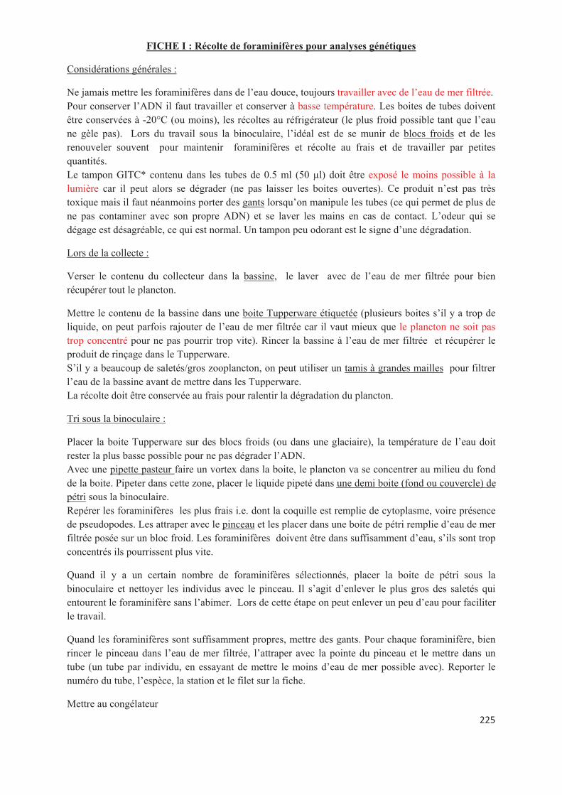
225
FICHE I : Récolte de foraminifères pour analyses génétiques
Considérations générales :
Ne jamais mettre les foraminifères dans de l’eau douce, toujours travailler avec de l’eau de mer filtrée.
Pour conserver l’ADN il faut travailler et conserver à basse température. Les boites de tubes doivent
être conservées à -20°C (ou moins), les récoltes au réfrigérateur (le plus froid possible tant que l’eau
ne gèle pas). Lors du travail sous la binoculaire, l’idéal est de se munir de blocs froids et de les
renouveler souvent pour maintenir foraminifères et récolte au frais et de travailler par petites
quantités.
Le tampon GITC* contenu dans les tubes de 0.5 ml (50 μl) doit être exposé le moins possible à la
lumière car il peut alors se dégrader (ne pas laisser les boites ouvertes). Ce produit n’est pas très
toxique mais il faut néanmoins porter des gants lorsqu’on manipule les tubes (ce qui permet de plus de
ne pas contaminer avec son propre ADN) et se laver les mains en cas de contact. L’odeur qui se
dégage est désagréable, ce qui est normal. Un tampon peu odorant est le signe d’une dégradation.
Lors de la collecte :
Verser le contenu du collecteur dans la bassine, le laver avec de l’eau de mer filtrée pour bien
récupérer tout le plancton.
Mettre le contenu de la bassine dans une boite Tupperware étiquetée (plusieurs boites s’il y a trop de
liquide, on peut parfois rajouter de l’eau de mer filtrée car il vaut mieux que le plancton ne soit pas
trop concentré pour ne pas pourrir trop vite). Rincer la bassine à l’eau de mer filtrée et récupérer le
produit de rinçage dans le Tupperware.
S’il y a beaucoup de saletés/gros zooplancton, on peut utiliser un tamis à grandes mailles pour filtrer
l’eau de la bassine avant de mettre dans les Tupperware.
La récolte doit être conservée au frais pour ralentir la dégradation du plancton.
Tri sous la binoculaire :
Placer la boite Tupperware sur des blocs froids (ou dans une glaciaire), la température de l’eau doit
rester la plus basse possible pour ne pas dégrader l’ADN.
Avec une pipette pasteur faire un vortex dans la boite, le plancton va se concentrer au milieu du fond
de la boite. Pipeter dans cette zone, placer le liquide pipeté dans une demi boite (fond ou couvercle) de
pétri sous la binoculaire.
Repérer les foraminifères les plus frais i.e. dont la coquille est remplie de cytoplasme, voire présence
de pseudopodes. Les attraper avec le pinceau et les placer dans une boite de pétri remplie d’eau de mer
filtrée posée sur un bloc froid. Les foraminifères doivent être dans suffisamment d’eau, s’ils sont trop
concentrés ils pourrissent plus vite.
Quand il y a un certain nombre de foraminifères sélectionnés, placer la boite de pétri sous la
binoculaire et nettoyer les individus avec le pinceau. Il s’agit d’enlever le plus gros des saletés qui
entourent le foraminifère sans l’abimer. Lors de cette étape on peut enlever un peu d’eau pour faciliter
le travail.
Quand les foraminifères sont suffisamment propres, mettre des gants. Pour chaque foraminifère, bien
rincer le pinceau dans l’eau de mer filtrée, l’attraper avec la pointe du pinceau et le mettre dans un
tube (un tube par individu, en essayant de mettre le moins d’eau de mer possible avec). Reporter le
numéro du tube, l’espèce, la station et le filet sur la fiche.
Mettre au congélateur
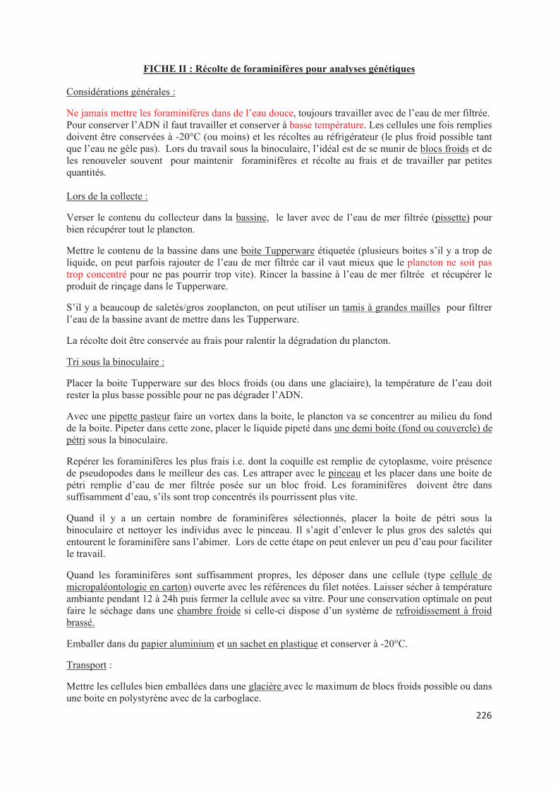
226
FICHE II : Récolte de foraminifères pour analyses génétiques
Considérations générales :
Ne jamais mettre les foraminifères dans de l’eau douce, toujours travailler avec de l’eau de mer filtrée.
Pour conserver l’ADN il faut travailler et conserver à basse température. Les cellules une fois remplies
doivent être conservées à -20°C (ou moins) et les récoltes au réfrigérateur (le plus froid possible tant
que l’eau ne gèle pas). Lors du travail sous la binoculaire, l’idéal est de se munir de blocs froids et de
les renouveler souvent pour maintenir foraminifères et récolte au frais et de travailler par petites
quantités.
Lors de la collecte :
Verser le contenu du collecteur dans la bassine, le laver avec de l’eau de mer filtrée (pissette) pour
bien récupérer tout le plancton.
Mettre le contenu de la bassine dans une boite Tupperware étiquetée (plusieurs boites s’il y a trop de
liquide, on peut parfois rajouter de l’eau de mer filtrée car il vaut mieux que le plancton ne soit pas
trop concentré pour ne pas pourrir trop vite). Rincer la bassine à l’eau de mer filtrée et récupérer le
produit de rinçage dans le Tupperware.
S’il y a beaucoup de saletés/gros zooplancton, on peut utiliser un tamis à grandes mailles pour filtrer
l’eau de la bassine avant de mettre dans les Tupperware.
La récolte doit être conservée au frais pour ralentir la dégradation du plancton.
Tri sous la binoculaire :
Placer la boite Tupperware sur des blocs froids (ou dans une glaciaire), la température de l’eau doit
rester la plus basse possible pour ne pas dégrader l’ADN.
Avec une pipette pasteur faire un vortex dans la boite, le plancton va se concentrer au milieu du fond
de la boite. Pipeter dans cette zone, placer le liquide pipeté dans une demi boite (fond ou couvercle) de
pétri sous la binoculaire.
Repérer les foraminifères les plus frais i.e. dont la coquille est remplie de cytoplasme, voire présence
de pseudopodes dans le meilleur des cas. Les attraper avec le pinceau et les placer dans une boite de
pétri remplie d’eau de mer filtrée posée sur un bloc froid. Les foraminifères doivent être dans
suffisamment d’eau, s’ils sont trop concentrés ils pourrissent plus vite.
Quand il y a un certain nombre de foraminifères sélectionnés, placer la boite de pétri sous la
binoculaire et nettoyer les individus avec le pinceau. Il s’agit d’enlever le plus gros des saletés qui
entourent le foraminifère sans l’abimer. Lors de cette étape on peut enlever un peu d’eau pour faciliter
le travail.
Quand les foraminifères sont suffisamment propres, les déposer dans une cellule (type cellule de
micropaléontologie en carton) ouverte avec les références du filet notées. Laisser sécher à température
ambiante pendant 12 à 24h puis fermer la cellule avec sa vitre. Pour une conservation optimale on peut
faire le séchage dans une chambre froide si celle-ci dispose d’un système de refroidissement à froid
brassé.
Emballer dans du papier aluminium et un sachet en plastique et conserver à -20°C.
Transport :
Mettre les cellules bien emballées dans une glacière avec le maximum de blocs froids possible ou dans
une boite en polystyrène avec de la carboglace.
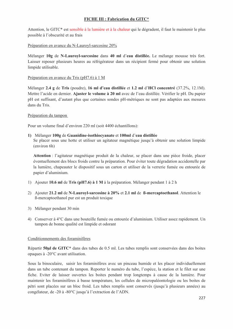
227
FICHE III : Fabrication du GITC*
Attention, le GITC* est sensible à la lumière et à la chaleur qui le dégradent, il faut le maintenir le plus
possible à l’obscurité et au frais
Préparation en avance du N-Lauroyl-sarcosine 20%
Mélanger 10g de N-Lauroyl-sarcosine dans 40 ml d’eau distillée. Le mélange mousse très fort.
Laisser reposer plusieurs heures au réfrigérateur dans un récipient fermé pour obtenir une solution
limpide utilisable.
Préparation en avance du Tris (pH7.6) à 1 M
Mélanger 2.4 g de Tris (poudre), 16 ml d’eau distillée et 1.2 ml d’HCl concentré (37.2%, 12.1M).
Mettre l’acide en dernier. Ajuster le volume à 20 ml avec de l’eau distillée. Vérifier le pH. Du papier
pH est suffisant, d’autant plus que certaines sondes pH-métriques ne sont pas adaptées aux mesures
dans du Tris.
Préparation du tampon
Pour un volume final d’environ 220 ml (soit 4400 échantillons):
1) Mélanger 100g de Guanidine-isothiocyanate et 100ml d’eau distillée
Se placer sous une hotte et utiliser un agitateur magnétique jusqu’à obtenir une solution limpide
(environ 6h)
Attention : l’agitateur magnétique produit de la chaleur, se placer dans une pièce froide, placer
éventuellement des blocs froids contre la préparation. Pour éviter toute dégradation accidentelle par
la lumière, chapeauter le dispositif sous un carton et utiliser de la verrerie fumée ou entourée de
papier d’aluminium.
1) Ajouter 10.6 ml de Tris (pH7.6) à 1 M à la préparation. Mélanger pendant 1 à 2 h
2) Ajouter 21.2 ml de N-Lauroyl-sarcosine à 20% et 2.1 ml de ß-mercaptoethanol. Attention le
ß-mercaptoethanol pur est un produit toxique
3) Mélanger pendant 30 min
4) Conserver à 4°C dans une bouteille fumée ou entourée d’aluminium. Utiliser assez rapidement. Un
tampon de bonne qualité est limpide et odorant
Conditionnements des foraminifères
Répartir 50μl de GITC* dans des tubes de 0.5 ml. Les tubes remplis sont conservées dans des boites
opaques à -20°C avant utilisation.
Sous la binoculaire, saisir les foraminifères avec un pinceau humide et les placer individuellement
dans un tube contenant du tampon. Reporter le numéro du tube, l’espèce, la station et le filet sur une
fiche. Eviter de laisser ouvertes les boites pendant trop longtemps à cause de la lumière. Pour
maintenir les foraminifères à basse température, les cellules de micropaléontologie ou les boites de
pétri sont placées sur un bloc froid. Les tubes remplis sont conservés (jusqu’à plusieurs années) au
congélateur, de -20 à -80°C jusqu’à l’extraction de l’ADN.
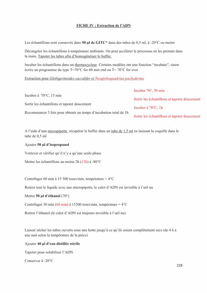
228
FICHE IV : Extraction de l’ADN
Les échantillons sont conservés dans 50 μl de GITC* dans des tubes de 0,5 ml, à -20°C ou moins
Décongeler les échantillons à température ambiante. On peut accélérer le processus en les prenant dans
la main. Tapoter les tubes afin d’homogénéiser le buffer.
Incuber les échantillons dans un thermocycleur. Certains modèles ont une fonction “incubate”, sinon
écrire un programme du type T=70°C for 60 min end ou T= 70°C for ever
Extraction pour Globigerinoides sacculifer et Neogloboquadrina pachyderma
Incuber à 70°C, 15 min
Sortir les échantillons et tapoter doucement
Recommencer 3 fois pour obtenir un temps d’incubation total de 1h
A l’aide d’une micropipette, récupérer le buffer dans un tube de 1,5 ml en laissant la coquille dans le
tube de 0,5 ml
Ajouter 50 μl d’isopropanol
Vortexer et vérifier qu’il n’y a qu’une seule phase
Mettre les échantillons au moins 2h (12h) à -80°C
Centrifuger 60 min à 15 300 tours/min, température = 4°C
Retirer tout le liquide avec une micropipette, le culot d’ADN est invisible à l’œil nu
Mettre 50 μl d’éthanol (70°)
Centrifuger 30 min (60 min) à 15300 tours/min, température = 4°C
Retirer l’éthanol (le culot d’ADN est toujours invisible à l’œil nu)
Laisser sécher les tubes ouverts sous une hotte jusqu’à ce qu’ils soient complètement secs (de 4 h à
une nuit selon la température de la pièce)
Ajouter 40 μl d’eau distillée stérile
Tapoter pour solubiliser l’ADN
Conserver à -20°C
Incuber 70°, 30 min
Sortir les échantillons et tapoter doucement
Incuber à 70°C, 1h
Sortir les échantillons et tapoter doucement
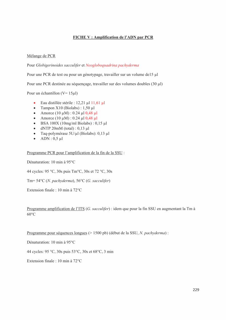
229
FICHE V : Amplification de l’ADN par PCR
Mélange de PCR
Pour Globigerinoides sacculifer et Neogloboquadrina pachyderma
Pour une PCR de test ou pour un génotypage, travailler sur un volume de15 μl
Pour une PCR destinée au séquençage, travailler sur des volumes doubles (30 μl)
Pour un échantillon (V= 15μl)
Eau distillée stérile : 12,21 μl 11,61 μl
Tampon X10 (Biolabs) : 1,50 μl
Amorce (10 μM) : 0.24 μl 0,48 μl
Amorce (10 μM) : 0.24 μl 0,48 μl
BSA 100X (10mg/ml Biolabs) : 0,15 μl
dNTP 20mM (total) : 0,13 μl
Taq-polymérase 5U/μl (Biolabs): 0,13 μl
ADN : 0,5 μl
Programme PCR pour l’amplification de la fin de la SSU :
Dénaturation: 10 min à 95°C
44 cycles: 95 °C, 30s puis Tm°C, 30s et 72 °C, 30s
Tm= 54°C (N. pachyderma), 56°C (G. sacculifer)
Extension finale : 10 min à 72°C
Programme amplification de l’ITS (G. sacculifer) : idem que pour la fin SSU en augmentant la Tm à
60°C
Programme pour séquences longues (> 1500 pb) (début de la SSU, N. pachyderma) :
Dénaturation: 10 min à 95°C
44 cycles: 95 °C, 30s puis 53°C, 30s et 68°C, 3 min
Extension finale : 10 min à 72°C
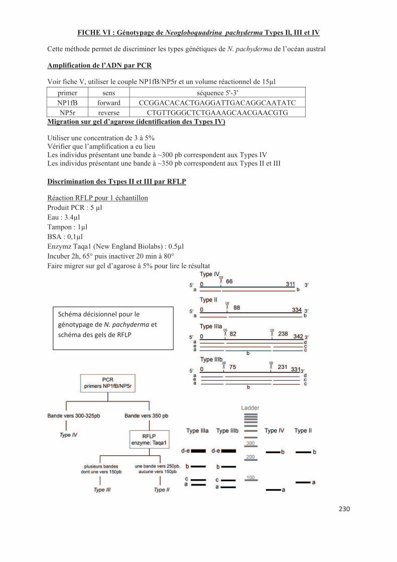
230
FICHE VI : Génotypage de Neogloboquadrina pachyderma Types Il, III et IV
Cette méthode permet de discriminer les types génétiques de N. pachyderma de l’océan austral
Amplification de l’ADN par PCR
Voir fiche V, utiliser le couple NP1fB/NP5r et un volume réactionnel de 15μl
primer sens séquence 5'-3'
NP1fB forward CCGGACACACTGAGGATTGACAGGCAATATC
NP5r reverse CTGTTGGGCTCTGAAAGCAACGAACGTG
Migration sur gel d’agarose (identification des Types IV)
Utiliser une concentration de 3 à 5%
Vérifier que l’amplification a eu lieu
Les individus présentant une bande à ~300 pb correspondent aux Types IV
Les individus présentant une bande à ~350 pb correspondent aux Types II et III
Discrimination des Types II et III par RFLP
Réaction RFLP pour 1 échantillon
Produit PCR : 5 μl
Eau : 3.4μl
Tampon : 1μl
BSA : 0,1μl
Enzymz Taqa1 (New England Biolabs) : 0.5μl
Incuber 2h, 65° puis inactiver 20 min à 80°
Faire migrer sur gel d’agarose à 5% pour lire le résultat
Schéma décisionnel pour le
génotypage de N. pachyderma et
schéma des gels de RFLP
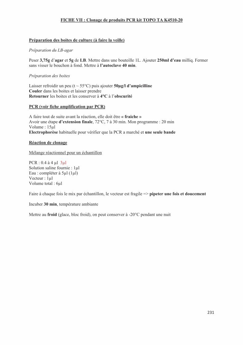
231
FICHE VII : Clonage de produits PCR kit TOPO TA K4510-20
Préparation des boites de culture (à faire la veille)
Préparation du LB-agar
Peser 3,75g d’agar et 5g de LB. Mettre dans une bouteille 1L. Ajouter 250ml d’eau milliq. Fermer
sans visser le bouchon à fond. Mettre à l’autoclave 40 min.
Préparation des boites
Laisser refroidir un peu (t ~ 55°C) puis ajouter 50μg/l d’ampicilline
Couler dans les boites et laisser prendre
Retourner les boites et les conserver à 4°C à l’obscurité
PCR (voir fiche amplification par PCR)
A faire tout de suite avant la réaction, elle doit être « fraiche »
Avoir une étape d’extension finale, 72°C, 7 à 30 min. Mon programme : 20 min
Volume : 15μl
Electrophorèse habituelle pour vérifier que la PCR a marché et une seule bande
Réaction de clonage
Mélange réactionnel pour un échantillon
PCR : 0.4 à 4 μl 3μl
Solution saline fournie : 1μl
Eau : compléter à 5μl (1μl)
Vecteur : 1μl
Volume total : 6μl
Faire à chaque fois le mix par échantillon, le vecteur est fragile => pipeter une fois et doucement
Incuber 30 min, température ambiante
Mettre au froid (glace, bloc froid), on peut conserver à -20°C pendant une nuit
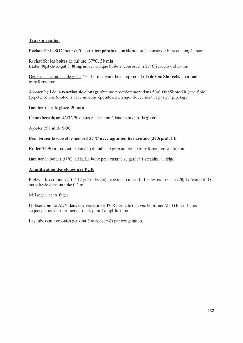
232
Transformation
Réchauffer le SOC pour qu’il soit à température ambiante ou le conserver hors du congélateur
Réchauffer les boites de culture, 37°C, 30 min
Etaler 40μl de X-gal à 40mg/ml sur chaque boite et conserver à 37°C jusqu’à utilisation
Dégeler dans un bac de glace (10-15 min avant la manip) une fiole de OneShotcells pour une
transformation
Ajouter 2 μl de la réaction de clonage obtenue précédemment dans 50μl OneShotcells (une fiole)
(pipeter le OneShotcells avec un cône épointé), mélanger doucement et pas par pipetage
Incuber dans la glace, 30 min
Choc thermique, 42°C, 30s, puis placer immédiatement dans la glace
Ajouter 250 μl de SOC
Bien fermer le tube et le mettre à 37°C avec agitation horizontale (200rpm), 1 h
Etaler 10-50 μl ou tout le contenu du tube de préparation de transformation sur la boite
Incuber la boite à 37°C, 12 h. La boite peut ensuite se garder 1 semaine au frigo.
Amplification des clones par PCR
Prélever les colonies (10 à 12 par individu) avec une pointe 10μl et les mettre dans 20μl d’eau milliQ
autoclavée dans un tube 0.2 ml
Mélanger, centrifuger
Utiliser comme ADN dans une réaction de PCR normale ou avec le primer M13 (fourni) puis
séquencer avec les primers utilisés pour l’amplification.
Les tubes eau+colonies peuvent être conservés par congélation.
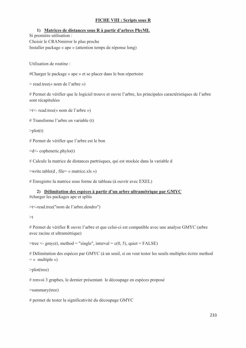
233
FICHE VIII : Scripts sous R
1) Matrices de distances sous R à partir d’arbres PhyML
Si première utilisation :
Choisir le CRANmirror le plus proche
Installer package « ape » (attention temps de réponse long)
Utilisation de routine :
#Charger le package « ape » et se placer dans le bon répertoire
> read.tree(« nom de l’arbre »)
# Permet de vérifier que le logiciel trouve et ouvre l’arbre, les principales caractéristiques de l’arbre
sont récapitulées
>t<- read.tree(« nom de l’arbre »)
# Transforme l’arbre en variable (t)
>plot(t)
# Permet de vérifier que l’arbre est le bon
>d<- cophenetic.phylo(t)
# Calcule la matrice de distances partrisques, qui est stockée dans la variable d
>write.table(d , file= « matrice.xls »)
# Enregistre la matrice sous forme de tableau (à ouvrir avec EXEL)
2) Délimitation des espèces à partir d’un arbre ultramétrique par GMYC
#charger les packages ape et splits
>t<-read.tree("nom de l’arbre.dendro")
>t
# Permet de vérifier R ouvre l’arbre et que celui-ci est compatible avec une analyse GMYC (arbre
avec racine et ultramétrique)
>tree <- gmyc(t, method = "single", interval = c(0, 5), quiet = FALSE)
# Délimitation des espèces par GMYC (à un seuil, si on veut tester les seuils multiples écrire method
= « multiple »)
>plot(tree)
# renvoi 3 graphes, le dernier présentant le découpage en espèces proposé
>summary(tree)
# permet de tester la significativité du découpage GMYC


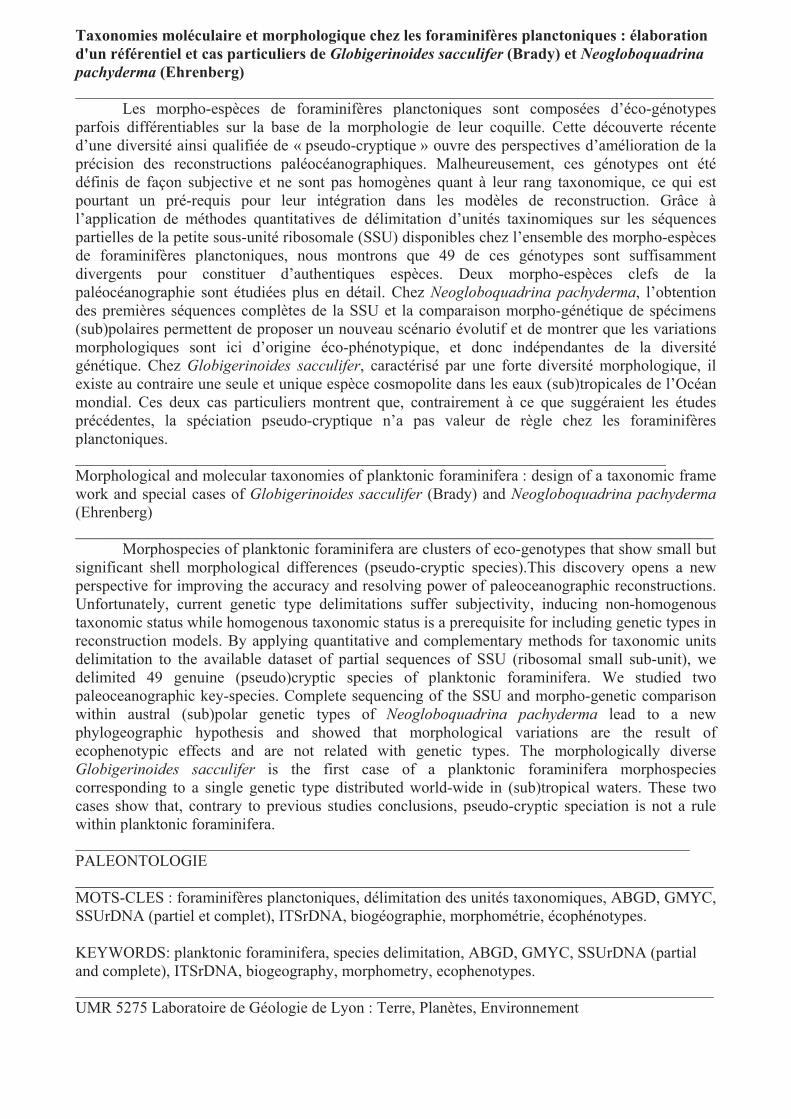
Taxonomies moléculaire et morphologique chez les foraminifères planctoniques : élaboration
d'un référentiel et cas particuliers de Globigerinoides sacculifer (Brady) et Neogloboquadrina
pachyderma (Ehrenberg)
________________________________________________________________________________
Les morpho-espèces de foraminifères planctoniques sont composées d’éco-génotypes
parfois différentiables sur la base de la morphologie de leur coquille. Cette découverte récente
d’une diversité ainsi qualifiée de « pseudo-cryptique » ouvre des perspectives d’amélioration de la
précision des reconstructions paléocéanographiques. Malheureusement, ces génotypes ont été
définis de façon subjective et ne sont pas homogènes quant à leur rang taxonomique, ce qui est
pourtant un pré-requis pour leur intégration dans les modèles de reconstruction. Grâce à
l’application de méthodes quantitatives de délimitation d’unités taxinomiques sur les séquences
partielles de la petite sous-unité ribosomale (SSU) disponibles chez l’ensemble des morpho-espèces
de foraminifères planctoniques, nous montrons que 49 de ces génotypes sont suffisamment
divergents pour constituer d’authentiques espèces. Deux morpho-espèces clefs de la
paléocéanographie sont étudiées plus en détail. Chez Neogloboquadrina pachyderma, l’obtention
des premières séquences complètes de la SSU et la comparaison morpho-génétique de spécimens
(sub)polaires permettent de proposer un nouveau scénario évolutif et de montrer que les variations
morphologiques sont ici d’origine éco-phénotypique, et donc indépendantes de la diversité
génétique. Chez Globigerinoides sacculifer, caractérisé par une forte diversité morphologique, il
existe au contraire une seule et unique espèce cosmopolite dans les eaux (sub)tropicales de l’Océan
mondial. Ces deux cas particuliers montrent que, contrairement à ce que suggéraient les études
précédentes, la spéciation pseudo-cryptique n’a pas valeur de règle chez les foraminifères
planctoniques.
__________________________________________________________________________
Morphological and molecular taxonomies of planktonic foraminifera : design of a taxonomic frame
work and special cases of Globigerinoides sacculifer (Brady) and Neogloboquadrina pachyderma
(Ehrenberg)
________________________________________________________________________________
Morphospecies of planktonic foraminifera are clusters of eco-genotypes that show small but
significant shell morphological differences (pseudo-cryptic species).This discovery opens a new
perspective for improving the accuracy and resolving power of paleoceanographic reconstructions.
Unfortunately, current genetic type delimitations suffer subjectivity, inducing non-homogenous
taxonomic status while homogenous taxonomic status is a prerequisite for including genetic types in
reconstruction models. By applying quantitative and complementary methods for taxonomic units
delimitation to the available dataset of partial sequences of SSU (ribosomal small sub-unit), we
delimited 49 genuine (pseudo)cryptic species of planktonic foraminifera. We studied two
paleoceanographic key-species. Complete sequencing of the SSU and morpho-genetic comparison
within austral (sub)polar genetic types of Neogloboquadrina pachyderma lead to a new
phylogeographic hypothesis and showed that morphological variations are the result of
ecophenotypic effects and are not related with genetic types. The morphologically diverse
Globigerinoides sacculifer is the first case of a planktonic foraminifera morphospecies
corresponding to a single genetic type distributed world-wide in (sub)tropical waters. These two
cases show that, contrary to previous studies conclusions, pseudo-cryptic speciation is not a rule
within planktonic foraminifera.
_____________________________________________________________________________
PALEONTOLOGIE
________________________________________________________________________________
MOTS-CLES : foraminifères planctoniques, délimitation des unités taxonomiques, ABGD, GMYC,
SSUrDNA (partiel et complet), ITSrDNA, biogéographie, morphométrie, écophénotypes.
KEYWORDS: planktonic foraminifera, species delimitation, ABGD, GMYC, SSUrDNA (partial
and complete), ITSrDNA, biogeography, morphometry, ecophenotypes.
________________________________________________________________________________
UMR 5275 Laboratoire de Géologie de Lyon : Terre, Planètes, Environnement