Tanagra Discretization for Supervised...
21
Tutorial R.R. 20 mai 2010 Page 1 sur 21 1 Topic Discretization of continuous features as preprocessing for supervised learning process. The discretization transforms a continuous attribute into a discrete one. To do that, it partitions the range into a set of intervals by defining a set of cut points. Thus we must answer to two questions to lead this data transformation: (1) how to determine the right number of intervals; (2) how to compute the cut points. The resolution is not necessarily in that sequence. The best discretization is the one performed by an expert domain. Indeed, he takes into account other information than those only provided by the available dataset. Unfortunately, this kind of approach is not always feasible because: often, the domain knowledge is not available or it does not allow to determine the appropriate discretization; the process cannot be automated to handle a large number of attributes. So, we are often forced to found the determination of the best discretization on a numerical process. Discretization of continuous featur Discretization of continuous featur Discretization of continuous featur Discretization of continuous features as preprocessing for supervised learning process es as preprocessing for supervised learning process es as preprocessing for supervised learning process es as preprocessing for supervised learning process. First, we must define the context in which we perform the transformation. Depending on the circumstances, it is clear that the process and criteria used will not be the same. In this tutorial, we are in the supervised learning framework. We perform the discretization prior to the learning process i.e. we transform the continuous predictive attributes into discrete before to present them to a supervised learning algorithm. In this context, the construction of intervals in which one and only one of the values of the target attribute is the most represented is desirable. The relevance of the computed solution is often evaluated through an impurity based or an entropy based functions. There are multiple motivations for performing discretization as a preprocessing step 1 : some learning methods do not handle continuous attributes; the data transformed in a set of intervals are more cognitively relevant for a human interpretation; the computation process goes faster with a reduced number of data, particularly when some attributes are suppressed from the representation space of the learning problem if it is impossible to find a relevant cutting; the discretization allows to discover non-linear relations – e.g. the infants and the elderly people are more sensitive to the illness, the relation between age and illness is then not linear – and that is why many authors propose to discretize the data even if the learning method can handle continuous attributes; lastly a discretization can harmonize the nature of the data if there are heterogeneous e.g., in text categorization, the attributes are a mix of numerical values and occurrence terms. There are several ways to distinguish the discretization algorithms. 1 F. Muhlenbach, R. Rakotomalala, « Discretization of Continuous Attributes », in Encyclopedia of Data Warehousing and Mining, John Wang (Ed.), pp. 397-402, 2005 (http://hal.archives-ouvertes.fr/hal-00383757/fr/ ).
Transcript of Tanagra Discretization for Supervised...

Tutorial R.R.
20 mai 2010 Page 1 sur 21
1 Topic
Discretization of continuous features as preprocessing for supervised learning process.
The discretization transforms a continuous attribute into a discrete one. To do that, it partitions the range into a set of intervals by defining a set of cut points. Thus we must answer to two questions to lead this data transformation: (1) how to determine the right number of intervals; (2) how to compute
the cut points. The resolution is not necessarily in that sequence.
The best discretization is the one performed by an expert domain. Indeed, he takes into account other information than those only provided by the available dataset. Unfortunately, this kind of approach is not always feasible because: often, the domain knowledge is not available or it does not allow to determine the appropriate discretization; the process cannot be automated to handle a large number
of attributes. So, we are often forced to found the determination of the best discretization on a numerical process.
Discretization of continuous featurDiscretization of continuous featurDiscretization of continuous featurDiscretization of continuous features as preprocessing for supervised learning processes as preprocessing for supervised learning processes as preprocessing for supervised learning processes as preprocessing for supervised learning process.... First, we must define the context in which we perform the transformation. Depending on the circumstances, it is clear that the process and criteria used will not be the same. In this tutorial, we are in the supervised learning framework. We perform the discretization prior to the learning process i.e. we transform the
continuous predictive attributes into discrete before to present them to a supervised learning algorithm. In this context, the construction of intervals in which one and only one of the values of the target attribute is the most represented is desirable. The relevance of the computed solution is often evaluated through an impurity based or an entropy based functions.
There are multiple motivations for performing discretization as a preprocessing step1: some learning
methods do not handle continuous attributes; the data transformed in a set of intervals are more cognitively relevant for a human interpretation; the computation process goes faster with a reduced number of data, particularly when some attributes are suppressed from the representation space of the learning problem if it is impossible to find a relevant cutting; the discretization allows to discover non-linear relations – e.g. the infants and the elderly people are more sensitive to the illness, the relation between age and illness is then not linear – and that is why many authors propose to
discretize the data even if the learning method can handle continuous attributes; lastly a discretization can harmonize the nature of the data if there are heterogeneous e.g., in text categorization, the attributes are a mix of numerical values and occurrence terms.
There are several ways to distinguish the discretization algorithms.
1 F. Muhlenbach, R. Rakotomalala, « Discretization of Continuous Attributes », in Encyclopedia of Data Warehousing and Mining, John Wang (Ed.), pp. 397-402, 2005 (http://hal.archives-ouvertes.fr/hal-00383757/fr/).

Tutorial R.R.
20 mai 2010 Page 2 sur 21
Univariate Univariate Univariate Univariate vs. Multivariatevs. Multivariatevs. Multivariatevs. Multivariate. The multivariate approaches discretize the continuous descriptors
simultaneously. These are the best solutions because the descriptors are often correlated. However, they are rarely used because they are time consuming, and above all, they are unavailable in the popular tools. On the other hand, the univariate approaches are very popular because they are fast and simple to use. But the cut points are defined individually for each continuous descriptor. We do not take into account the eventual interdependence between them.
Unsupervised vs. SupervisedUnsupervised vs. SupervisedUnsupervised vs. SupervisedUnsupervised vs. Supervised. The unsupervised approaches make use only of the attribute to discretize to define the cut points. Often, but not always2, the number of intervals is a parameter of the algorithm. Their main advantage is that we can use them in any context, including the supervised learning context. Their main drawback is that they are not especially intended to a supervised learning, they do not use the information provided by the target attribute. The supervised approaches use explicitly the target attribute during the discretization process. They often provide at the same time
both the number of intervals and the cut points. They are the most interesting ones in our context.
In this tutorial, we use only the univariate approaches. We compare the behavior of the supervised and the unsupervised algorithms on an artificial dataset. We use several tools for that: Tanagra 1.4.35, Sipina 3.3, R 2.9.2 (package dprep), Weka 3.6.0, Knime 2.1.1, Orange 2.0b and RapidMiner 4.6.0. We highlight the settings and the reading of the results.
About Tanagra, we show how to utilize the transformed variables after the discretization process. Almost all the tools discussed in this tutorial provide the same functionality.
2 There are various formulas to determine automatically the number of intervals. They are mainly based on the sample size, and sometimes on the range of the values and the standard deviation (http://www.info.univ-angers.fr/~gh/wstat/discr.php) :
ApproachApproachApproachApproach FormulaFormulaFormulaFormula
Brooks-Carruthers ( )n10log5×
Huntsberger ( )n10log332.31 ×+
Sturges ( )1log2 +n
Scott ( )315.3 −××
−n
ab
σ
Freedman-Diaconis ( )312 −××
−nq
ab
Where n is the sample size ; b the maximum ; a the minimum ; σ the standard deviation ; q the interquartile
range.

Tutorial R.R.
20 mai 2010 Page 3 sur 21
2 Dataset
We use an artificial dataset in this tutorial. The target attribute is binary (positive vs. negative). The 4 continuous predictive variables are generated according various conditional distributions.
Such experimentation is usual in the publications3. Indeed, knowing the characteristics of the data, we know the proper solutions. First, we give here the distribution of the attributes without taking into account the class membership (Figure 1).
x1
Den
sité
0.00
0.05
0.10
0.15
0.20
0.25
2 4 6 8 10
x2
Den
sité
0.0
0.1
0.2
0.3
0.4
2 4 6 8
x3
De
nsité
0.00
0.05
0.10
0.15
0 5 10 15
x4
De
nsité
0.00
0.02
0.04
0.06
0.08
0.10
5 10 15
Figure Figure Figure Figure 1111 –––– Unconditional distribution of the predictive attributesUnconditional distribution of the predictive attributesUnconditional distribution of the predictive attributesUnconditional distribution of the predictive attributes
It is difficult to visually detect the cut points using these density functions. Even if it seems there are
several modes in some cases, we do not know if these modes are associated to different class values or not.
For the same variables, we draw the density function according the class membership (Figure 2). The conclusions are very different. Excluding the variable X2 for which the conditional densities functions are not discernible, for the others, we note that we can found some cut points in order to define intervals associated to one of the values of the target attribute.
3 E.g. M. Ismail, V. Ciesielski, “An Empirical Investigation of the Impact of Discretization on Common Data Distributions”, in Design and Application of hybrid intelligent systems, 2003; http://portal.acm.org/citation.cfm?id=998117&dl=GUIDE&coll=GUIDE&CFID=88985182&CFTOKEN=88220030

Tutorial R.R.
20 mai 2010 Page 4 sur 21
x1
Den
sité
0.0
0.2
0.4
0.6
0.8
2 4 6 8
x2
Den
sité
0.0
0.1
0.2
0.3
0.4
0 2 4 6 8
x3
Den
sité
0.0
0.1
0.2
0.3
0.4
0 5 10 15 20
x4D
ensi
té
0.00
0.05
0.10
0.15
0 5 10 15
Figure Figure Figure Figure 2222 ---- Conditional distributions of the predic Conditional distributions of the predic Conditional distributions of the predic Conditional distributions of the predictive attributestive attributestive attributestive attributes
Thus, in the supervised learning context, the utilization of the information provided by the target attribute during the discretization process is essential.
In what follows, we will use both the unsupervised and supervised techniques implemented in several data mining tools. For the former, we focus mainly on equal width intervals and equal frequency intervals approaches4. Both require the indication of the number of intervals. We will set it to 5. We set
a fairly large number of intervals in order to obtain relatively pure intervals according to the target variable, although we have no guarantee on that. About the supervised approaches, we use the default settings. The algorithm detects automatically the appropriate number of intervals and the cut points.
The data file is in the Weka file format (ARFF5), it is available on line6.
3 Discretization in Tanagra
Importing the data fileImporting the data fileImporting the data fileImporting the data file. We launch TANAGRA. We create a new diagram by clicking on the FILE / NEW menu. We import the data file “datadatadatadata----discretization.arfdiscretization.arfdiscretization.arfdiscretization.arfffff”.
4 http://robotics.stanford.edu/users/sahami/papers-dir/disc.pdf 5 http://tutoriels-data-mining.blogspot.com/2008/03/importer-un-fichier-weka-dans-tanagra.html 6 http://eric.univ-lyon2.fr/~ricco/tanagra/fichiers/data-discretization.arff

Tutorial R.R.
20 mai 2010 Page 5 sur 21
Unsupervised discretizationUnsupervised discretizationUnsupervised discretizationUnsupervised discretization. To discretize with the “equal width intervals” approach, we must specify the variables to analyze with the DEFINE STATUS component.
Then, we insert the EqWidthEqWidthEqWidthEqWidthDiscDiscDiscDisc tool (FEATURE CONSTRUCTION)7. With the default settings, the variables are discretized into 5 intervals. We can modify this parameter. We click on the VIEW menu to obtain the computed cut points.
7 The other available tool is EqFreqDiscEqFreqDiscEqFreqDiscEqFreqDisc, equal frequency intervals discretization.

Tutorial R.R.
20 mai 2010 Page 6 sur 21
Of course, if we consider the data characteristics (Figure 2), the discretization into 5 intervals is not appropriated in the majority of cases. We note however than some cut points are, a little by chance, suitable in some situations. For instance, the cut point 6.47 is not too bad for the variable X1. But, on the other hand, the others cut points are irrelevant. This is the main drawback of this approach. If we set a large number of intervals, some cut points are maybe interesting, but we increase also the risk of
data fragmentation, increasing at the same time the variance of the induced classifier.
Conversely, it is clear that there is no discretization possible for X2. The procedure provides us four cut points that are totally irrelevant.
Supervised learning process from the transformed variablesSupervised learning process from the transformed variablesSupervised learning process from the transformed variablesSupervised learning process from the transformed variables. To use the transformed variables, we insert the DEFINE STATUS tool, we set them as INPUT. The target attribute is Y.

Tutorial R.R.
20 mai 2010 Page 7 sur 21
Then we add the decision list algorithm which induces ordered rules (SPV LEARNING – see
http://data-mining-tutorials.blogspot.com/2010/02/supervised-rule-induction-software.html). It cannot handle directly continuous descriptors. The discretization preprocessing step is needed here.
The classifier is rather good according to the resubstitution error rate. It is not surprising because we see before that in some situations, the discretization can find by chance some good cut points if we set a large number of intervals. But, when we consider carefully the ruleset, we note that we obtain unnecessary rules in the classifier. For instance, we observe that we need two rules (n°2 and n°3) to
assign an instance to the negative class value, whereas one rule would have been enough e.g. « ELSE IF X1 ≥ 6.47 THEN Y = NEGATIVE ». The cut point “X1 = 7.748” is irrelevant.
Supervised discretizationSupervised discretizationSupervised discretizationSupervised discretization. To perform a supervised discretization, we set X1…X4 as INPUT, and Y as TARGET with the DEFINE STATUS tool.

Tutorial R.R.
20 mai 2010 Page 8 sur 21
We specify the target attribute here because the descriptors will be discretized with respect to Y.
We add the MDLPC component (FEATURE CONSTRUCTION) which implements a very popular approach (U. Fayyad et K. Irani, « Multi-interval discretization of continuous-valued attributes for classification
learning », in Proc. of IJCAI, pp.1022-1027, 1993). We click on the VIEW menu.
The approach detects the good number of intervals according the variables. Sometimes, the
discretization is not performed if the processing is not relevant. The method is singularly efficient on our artificial dataset. Among others, it detects rightly that the discretization is not feasible for X2.
Supervised learning process from the transformed variablesSupervised learning process from the transformed variablesSupervised learning process from the transformed variablesSupervised learning process from the transformed variables. Here again, we perform the induction of decision list on the transformed descriptors.

Tutorial R.R.
20 mai 2010 Page 9 sur 21
The obtained classifier is as good as (resubstitution error rate) the preceding one, but it is simpler with
fewer rules. In our dataset, the descriptor X1 is enough to build an efficient classifier.
Geometrical interpretationGeometrical interpretationGeometrical interpretationGeometrical interpretation. If we plot the points in a scatter diagram defined by (X1, X2), we observe indeed that X1 is enough to separate perfectly the individuals from different groups.
(X1) x1 vs. (X2) x2 by (Y) y
positive negative
9876543
7
6
5
4
3
2
(X1) x1 vs. (X2) x2 by (Y) y
positive negative
9876543
7
6
5
4
3
2
4 Discretization in SIPINA
Importing the data fileImporting the data fileImporting the data fileImporting the data file. We launch SIPINA (http://eric.univ-lyon2.fr/~ricco/sipina.html). We import the data file by clicking on the FILE / OPEN menu. We select datadatadatadata----discretization.arffdiscretization.arffdiscretization.arffdiscretization.arff.
Tutorial R.R.
20 mai 2010 Page 10 sur 21
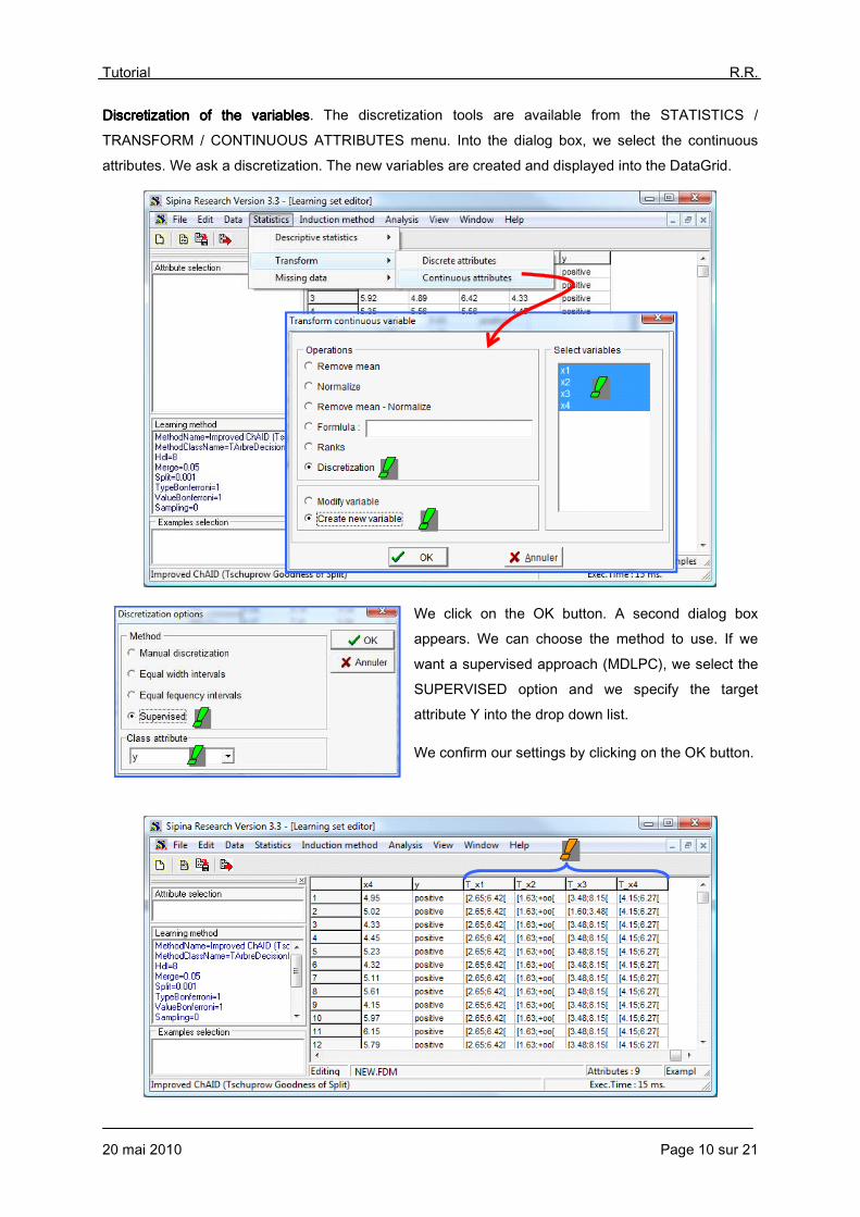
Discretization of the variablesDiscretization of the variablesDiscretization of the variablesDiscretization of the variables. The discretization tools are available from the STATISTICS /
TRANSFORM / CONTINUOUS ATTRIBUTES menu. Into the dialog box, we select the continuous attributes. We ask a discretization. The new variables are created and displayed into the DataGrid.
We click on the OK button. A second dialog box appears. We can choose the method to use. If we
want a supervised approach (MDLPC), we select the SUPERVISED option and we specify the target attribute Y into the drop down list.
We confirm our settings by clicking on the OK button.

Tutorial R.R.
20 mai 2010 Page 11 sur 21
The transformed attributes are now displayed into the data grid. The results (number of intervals and
cut points) are the same as those of Tanagra.
NoteNoteNoteNote: We can manually discretize the variables in Sipina (MANUAL DISCRETIZATION). We enumerate the cut points by separating them with ";" in the dialog settings.
5 Discretization in R (« dprep » package)
The dprepdprepdprepdprep package for R (http://www.r-project.org/) incorporates various approaches for the discretization process.
We set the following commands for the importation of the data file.
#load the dataset library(RWeka) donnees <- read.arff(file="data-discretization.arff") summary(donnees)
Some descriptive statistics indicators allows to check the data integrity.
Equal width discretizationEqual width discretizationEqual width discretizationEqual width discretization. For the equal width discretization process, we set the following commands.
#discretization library(dprep) #equal-width discretization new.donnees <- disc.ew(donnees,1:4) summary(new.donnees)
The number of intervals is automatically determined with the Scott’s formula (see above).
E.g. For X1, we have 100=n ; 022.9=b ; 654.2=a ; 484.1=σ . We obtain

Tutorial R.R.
20 mai 2010 Page 12 sur 21
( ) 69.55.3 31
=××
−−n
ab
σ
The value is rounded to 6.
Supervised discretizationSupervised discretizationSupervised discretizationSupervised discretization with with with with MDLPCMDLPCMDLPCMDLPC. Even if the help file does not quote explicitly the Fayyad and Irani's paper, it seems that the supervised algorithm relies on a very similar approach.
#supervised discretization (mdl) new.spv1.donnees <- disc.mentr(donnees,1:5) summary(new.spv1.donnees)
A new data.frame is generated. The function displays the number of intervals and the cut points.
Supervised discretization withSupervised discretization withSupervised discretization withSupervised discretization with CHI CHI CHI CHI----MERGEMERGEMERGEMERGE. The “dprep” package incorporates another supervised discretization technique. This is the CHI-MERGE method (Kerber, 1992). In comparison with MDLPC, it is a bottom-up approach. It starts with the purest discretization (in the worst case, we have an
individual into each interval). It tries to merge the adjacent intervals if the distribution of the target attributes is not significantly different. The process is stopped when none merging is possible. Unfortunately, this approach relies heavily on the parameter alpha (the significance level of the test). To define the good value according the domain or the data characteristics is difficult.
We set the following commands.
#supervised discretization (chi-merge) new.spv2.donnees <- chiMerge(donnees,1:4,alpha=0.1) summary(new.spv2.donnees)
The variable X2, for which it is not possible to find an efficient solution, is discretized into 35 intervals (!); the variable X4 is discretized into 9 intervals.

Tutorial R.R.
20 mai 2010 Page 13 sur 21
We try to decrease the significance level to favor the merging. The solution for X2 is improved. But the number of intervals remains too high for several variables.
The contingency tables between the target variable and recoded descriptors (X3, X4) show that
merging operations are still necessary.
6 Discretization in Weka
We use Weka (http://www.cs.waikato.ac.nz/ml/weka/) in EXPLORER mode. Into the PREPROCESS tab, we load the data file by clicking on the OPEN FILE button.

Tutorial R.R.
20 mai 2010 Page 14 sur 21
Weka displays automatically the distributions of the variables conditionally to the target attribute (the
last column of the data file).
To perform the discretization process, we click on the CHOOSE button (FILTER), we select the DISCRETIZE tool in the SUPERVISED branch.
The tool implements the MDLPC approach (Fayyad and Irani, 1993). We click on the APPLY button. All the continuous variables (FIRST � LAST) are discretized.

Tutorial R.R.
20 mai 2010 Page 15 sur 21
The discretized variables are substituted to the previous ones. For each interval, we obtain both the number of intervals, the cut points, the number of instances, the classes distribution. E.g. for X1 ≤ 6.416414, we have 50 instances, they are all positives.
7 Discretization in Knime
We create a new « Workflow » under Knime (http://www.knime.org/).
We import the data file with the ARFF READER component. The CONFIGURE contextual menu allows to select the file. We click on the EXECUTE menu to read the file.

Tutorial R.R.
20 mai 2010 Page 16 sur 21
Manual discretizationManual discretizationManual discretizationManual discretization. The NUMERIC BINNER tool allows to specify manually the cut points (and thus
the number of intervals). We add the component into the workflow, we click on the CONFIGURE menu.
For each variable, we can define the number of intervals and the cut points. The transformed variables are available behind the component into the workflow. We can use them with the other tools, especially with the machine learning algorithms. Here, we visualize the new columns using the INTERACTIVE TABLE component.
Supervised discretizationSupervised discretizationSupervised discretizationSupervised discretization. The CAIM BINNER supervised discretization tool of Knime is based on the CAIM algorithm (Kurgan et Cios, 2004; http://citeseer.ist.psu.edu/kurgan04caim.html). Let us analyze
the behavior of this approach on our dataset.

Tutorial R.R.
20 mai 2010 Page 17 sur 21
Compared to MDLPC which found the good solutions for each variable, CAIM provides wrongly 3 intervals for the variable X2 (instead of 0) and 3 for X4 (instead of 4). But this is just one example among many others. It would require large-scale experiments to really assess the behavior of the
algorithm.
8 Discretization in Orange
We import the data file with the FILE tool under Orange (http://www.ailab.si/orange/).
NoteNoteNoteNote: Orange does not handle the ARFF file, I do not why. Thus we used the tab delimited file format.

Tutorial R.R.
20 mai 2010 Page 18 sur 21
DiscrDiscrDiscrDiscreeeetitititizzzzationationationation. The DISCRETIZE tool (DATA tab) allows to perform a discretization process according
various methods. The tool is rich with many options. We select the ENTROPY-MDL DISCRETIZATION which corresponds to the Fayyad and Irani’s MDLPC approach according the user’s guide (http://www.ailab.si/orange/doc/ofb/o_categorization.htm).
We click on the REPORT button to obtain the results.
The results are roughly the same than those of Tanagra or Weka. But the cut points are slightly different. This has no incidence on the learning method implemented subsequently.

Tutorial R.R.
20 mai 2010 Page 19 sur 21
Of course, the transformed variables are available behind the component.
9 Discretization in RapidMiner
We create a new diagram (FILE / NEW) with RapidMiner (http://rapid-i.com/content/view/181/196/).
We insert the ARFF EXAMPLES SOURCE tool.
We specify the data file name datadatadatadata----discretization.arffdiscretization.arffdiscretization.arffdiscretization.arff and the target variable yyyy.
We must search in the submenus to find the tools for discretization.

Tutorial R.R.
20 mai 2010 Page 20 sur 21
We select the MINIMAL ENTROPY PARTITIONNING. The documentation gives two references (Fayyad and Irani, 1993; Dougherty et al., 1995). But we have not the details of the used algorithm. We click on the RUN button into the toolbar to perform the discretization.
RapidMiner provides some indications about the process. Into the RANGE column, we obtain the
number of intervals and the cut points. We note that the software has rejected the discretization of X1 (wrongly) and X2 (rightly). About X3 and X4, the number of intervals corresponds to those of Weka and Tanagra. But some cut points are quite different, however.

Tutorial R.R.
20 mai 2010 Page 21 sur 21
10 Conclusion
The discretization of continuous variables is a usual task in the data mining process. If the unsupervised methods are fairly well known by practitioners, it is not the case for the supervised approaches. Yet, they exist and they provide relevant results in the vast majority of cases.
Finally, there is a very simple alternative for cutting a continuous
variable into classes in a supervised framework: we build a decision tree by specifying a single predictive variable, the one you want to discretize. We note
indeed that the popular MDLPC (Fayyad and Irani, 1993) approach which performs a top down partitioning of the range of the values operates like a decision tree algorithm.
To check this idea, we use the J48 algorithm of the RWeka package under R. We create a decision tree by using in turn each continuous attribute.
The results are very similar to those of the MDLPC algorithm. We obtain the same number of intervals. The cut points however are slightly different. This is because the decision tree
algorithm uses another goodness of split criterion (Quinlan’s Gain
ratio, 1993) during the process.
Whatever, we obtained valid solutions with the decision tree algorithm.