Data visualization, feature reduction and cluster...

Ricco Rakotomalala

Tutoriels Tanagra - http://tutoriels-data-mining.blogspot.fr/ 1

Ricco RAKOTOMALALAUniversité Lumière Lyon 2

Data visualization, feature reduction and cluster analysis

http://tutoriels-data-mining.blogspot.fr/

Ricco Rakotomalala


Outline

1. SOM – Kohonen map – Kohonen network

2. Learning algorithm

3. Data visualization

4. Assigning a new instance to a node

5. Tools – Case study (R, Tanagra)

6. Cluster analysis from SOM

7. Supervised self-organizing map

8. Conclusion

9. References


Ricco Rakotomalala


Kohonen network


Ricco Rakotomalala


Self-organizing mapKohonen map, Kohonen network

Biological

metaphor

Our brain is subdivided into specialized areas, they

specifically respond to certain stimuli i.e. stimuli of the

same kind activate a particular region of the brain.

Kohonen

map

The idea is transposed to a competitive unsupervised

learning system where the input space is "mapped" in

a small (often rectangular) space with the following

principle: similar individuals in the initial space will be

projected into the same neuron or, at least, in

neighboring neurons in the output space (preservation

of proximity).

SOM serves both to the dimensionality reduction, data visualization and

cluster analysis (clustering).


Ricco Rakotomalala


SOM - Architecture

Input space, description of the dataset into the

original representation space (vector with p values

[for p variables]).

•To each neuron (node) corresponds a set of

instances from the dataset.

•To each neuron (node) is associated a vector of

weights (codebook) which describes the typical

profile of the neuron.

•The positions of the neurons in the map are

important i.e. (1) two neighboring neurons have

similar codebook; (2) a set of contiguous neurons

correspond to a particular pattern in the data.

The connections between the input and output

layers indicate the relationships between the input

and output vectors.


Ricco Rakotomalala


SOM – Example (1)

Cars dataset.

p = 6 variables.

A neuron a "small" cars (4 cars above), poorly performing, with bad

power-to-weight ratio.

“Weights” (codebook) of the node


Ricco Rakotomalala


SOM – Example (2)

Mapping plot

A rectangular grid with (3 x 3) neurons

Codebooks plot

We have both a visualization tool (the proximity between the neurons has

meaning) and clustering tool (we have a first organization of the data in groups).


Ricco Rakotomalala


SOM and PCA (principal component analysis)

PCA is a popular statistical method for dimensionality reduction and data visualization.

Mapping plot Biplot

We can see roughly the same proximities. But there is a linear constraint in the

PCA (the components are linear combinations of the initial variables) that does

not exist in SOM. This constraint, as well as the orthogonality between the

factors, can be a drawback for the handling of nonlinear problems (see the

example at Wikipedia). Unlike PCA, the output of SOM is in 2D space (very often).


https://en.wikipedia.org/wiki/Self-organizing_map

Ricco Rakotomalala


SOM Architecture and neighborhood

Rectangular grid - Rectangular neighborhood

First-order neighborhood

Second-order neighborhood

The notion of neighborhood is essential in SOM,

especially for the updating of weights and their

propagation during the learning process.

Note: an unidimensional map (vector) is possible

Hexagonal grid - Circular neighborhood

First-order neighborhoodSecond-order neighborhood


Ricco Rakotomalala


Initialization, competition, cooperation, adaptation


Ricco Rakotomalala


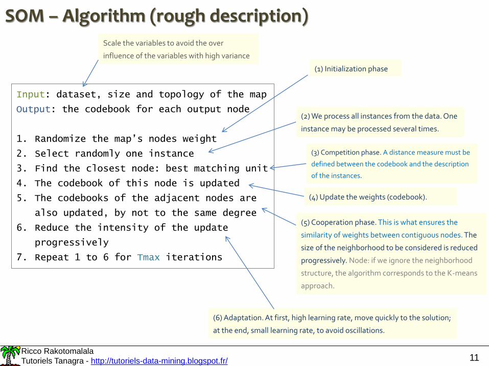
SOM – Algorithm (rough description)

Input: dataset, size and topology of the map

Output: the codebook for each output node

1. Randomize the map’s nodes weight

2. Select randomly one instance

3. Find the closest node: best matching unit

4. The codebook of this node is updated

5. The codebooks of the adjacent nodes are

also updated, by not to the same degree

6. Reduce the intensity of the update

progressively

7. Repeat 1 to 6 for Tmax iterations

Scale the variables to avoid the over

influence of the variables with high variance

(1) Initialization phase

(2) We process all instances from the data. One

instance may be processed several times.

(3) Competition phase. A distance measure must be

defined between the codebook and the description

of the instances.

(5) Cooperation phase. This is what ensures the

similarity of weights between contiguous nodes. The

size of the neighborhood to be considered is reduced

progressively. Node: if we ignore the neighborhood

structure, the algorithm corresponds to the K-means

approach.

(6) Adaptation. At first, high learning rate, move quickly to the solution;

at the end, small learning rate, to avoid oscillations.

(4) Update the weights (codebook).


Ricco Rakotomalala


SOM – Algorithm – Details (1)

Weight update rule for a node j,

knowing that j* is the winning node

xjwjjhjwjw ttttt )(*),()()(1

(a) h() is a neighborhood function. Its amplitude (spatial

width of the kernel) decreases according to the step

index (t)

)(2

*),(exp*),(

2

2

t

jjdjjht

Où

Tmaxexp)( 0

tt

(b) ε is the learning rate. Its value

decreases according the step index (t)

Implementations differ from one software to another, but the guiding ideas are there.

Gradual reduction: of the size of the neighborhood to consider, of the learning rate.

Tmaxexp0

tt

d(j,j*) is the distance

between the nodes j

and j* on the map

σ0, ε0 and Tmax are parameters of the algorithm

Input: dataset, size and topology

of the map

Output: the codebook for each

output node

1. Randomize the map’s nodes

weight

2. Select randomly one instance

3. Find the closest node: best

matching unit

4. The codebook of this node is

updated

5. The codebooks of the adjacent

nodes are also updated, by not

to the same degree

6. Reduce the intensity of the

update progressively

7. Repeat 1 to 6 for Tmax

iterations


Ricco Rakotomalala


SOM – Algorithm – Details (2)

Influence of the neighborhood distance [d(j,j*) =

0, …, 5 (t = 0)] on the neighborhood function

Decreasing of the influence of the neighborhood

according the step index (t = 0, …, 20)

Tmaxexp)( 0

tt

)0(2

*),(exp*),(

2

2

0

jjdjjh

)20(2

*),(exp*),(

2

2

20

jjdjjh

σ0 = 1.5, Tmax = 20

First order

neighborhood: learning

rate= 0.8 ; second order

: 0.41 ; etc.

The influence on the

neighbors decreases over

the iterations. For t = 20,

only the first order

neighborhood is affected

by the update process.

Influence of the neighborhood distance [d(j,j*) =

0, …, 5 (t = 20)] on the neighborhood function


Ricco Rakotomalala


SOM provides various very interesting data

visualization scenarios


Ricco Rakotomalala


Visualization – Sample size, list of individuals

Labels of individuals, impracticable when we

deal with large dataset (number of instances).

Color code. It enables to identify areas with a high

density of individuals. Useful on large databases.


Ricco Rakotomalala


Visualization – Distance between nodes (U-matrix)

SOM

PCA (Factors 1 and 2)

Distance to the immediate neighbors of each node. E.g. the node

including « Audi 100 », « Peugeot 504 » and « Princess 1800 » is close to its

immediate neighbors (V1, V2 and V3). See the position of the groups in

the representation space defined by the two first components of the PCA.

A

A

V1

V2V3

V1

V2

V3

Euclidean distance between codebooks of neighboring nodes.


Ricco Rakotomalala


Visualization – Characterization by variablesObjective: Understand what characterizes the regions of the topological map

Impracticable when the number of

variables is high.We can have a global view. But the larger number of

the graphs does not make things easy. The correlation

ratio can be used to determine the overall contrast for

each variable on the output nodes.

Heatmaps

Codebooks

Individuals

Comparing the conditional averages


Ricco Rakotomalala


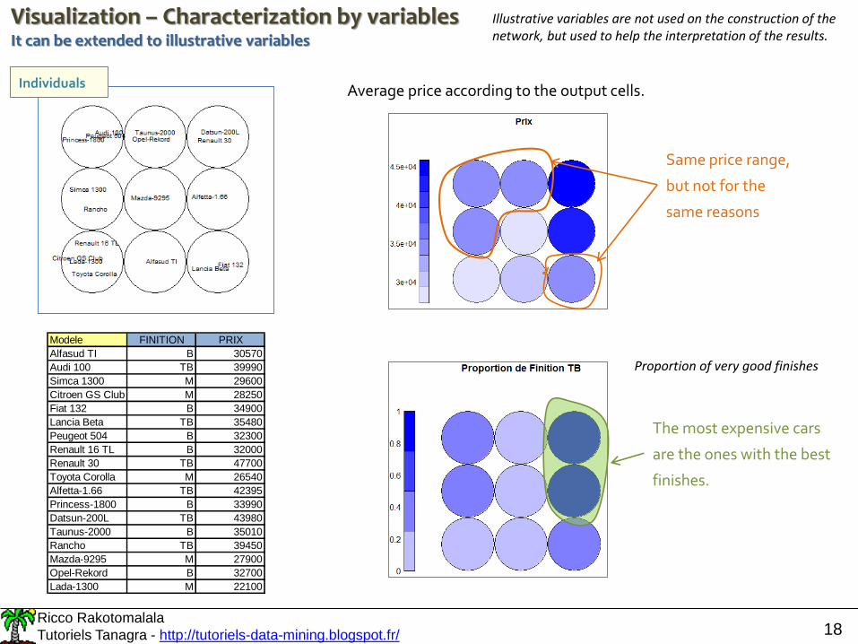
Visualization – Characterization by variablesIt can be extended to illustrative variables

Individuals

Modele FINITION PRIX

Alfasud TI B 30570

Audi 100 TB 39990

Simca 1300 M 29600

Citroen GS Club M 28250

Fiat 132 B 34900

Lancia Beta TB 35480

Peugeot 504 B 32300

Renault 16 TL B 32000

Renault 30 TB 47700

Toyota Corolla M 26540

Alfetta-1.66 TB 42395

Princess-1800 B 33990

Datsun-200L TB 43980

Taunus-2000 B 35010

Rancho TB 39450

Mazda-9295 M 27900

Opel-Rekord B 32700

Lada-1300 M 22100

Average price according to the output cells.

Same price range,

but not for the

same reasons

The most expensive cars

are the ones with the best

finishes.

Illustrative variables are not used on the construction of the network, but used to help the interpretation of the results.

Proportion of very good finishes


Ricco Rakotomalala


Assignment to the most closest node


Ricco Rakotomalala


Predicting the node membership of a new instance

Submit the new instant to the input layer, with

possibly the data transformation used during the

learning phase (standardization,...).

Identify the output neuron (winning neuron) in the

sense of the smallest distance to the codebook of

the neurons (e.g. Euclidean distance).

Predicting the node membership of a new instance. This operation will be

really essential when we use the SOM network for the cluster analysis.


Ricco Rakotomalala


R (Kohonen package), Tanagra


https://cran.r-project.org/web/packages/kohonen/index.html

Ricco Rakotomalala


#package kohonen

library(kohonen)

#wines dataset, included in the package (n = 177, p = 13)

data(wines)

print(summary(wines))

#Z – standardization of the variables

Z <- scale(wines,center=T,scale=T)

#learning phase – hexagonal grid

grille <- som(Z,grid=somgrid(5,4,"hexagonal"))

#shades of blue colors

degrade.bleu <- function(n){

return(rgb(0,0.4,1,alpha=seq(1/n,1,1/n)))

}

#plot number of instances per node

plot(grille,type="count",palette.name=degrade.bleu)

#plot the codebook

plot(grille,type="codes",codeRendering = "segments")

R – « kohonen » package


Ricco Rakotomalala


Tanagra – « Kohonen – SOM » component

Number of instances per node

CodebooksThe tool can standardize

automatically the variables


Ricco Rakotomalala


Two step clustering – Large dataset processing


Ricco Rakotomalala


SOM: we can perform directly a clustering by limiting the number of output nodes

But nothing really distinguishes the approach from the K-means method in this case.

Cluster analysisAlso called: clustering, unsupervised learning, numerical taxonomy, typological analysis

Goal: Identifying the set of objects with similar characteristics

We want that:

(1) The objects in the same group are more similar to each other

(2) Thant to those in other groups

For what purpose?

Identify underlying structures in the data

Summarize behaviors or characteristics

Assign new individuals to groups

Identify totally atypical objects

Modele Pr ix Cylindree Puissance Poids Consom m ation Groupe

Daihatsu Cuore 11600 846 32 650 5.7

Suzuki Swift 1.0 GLS 12490 993 39 790 5.8

Fiat Panda Mam bo L 10450 899 29 730 6.1

VW Polo 1.4 60 17140 1390 44 955 6.5

Opel Corsa 1.2i Eco 14825 1195 33 895 6.8

Subaru Vivio 4WD 13730 658 32 740 6.8

Toyota Corolla 19490 1331 55 1010 7.1

Opel As tra 1.6i 16V 25000 1597 74 1080 7.4

Peugeot 306 XS 108 22350 1761 74 1100 9

Renault Safrane 2.2. V 36600 2165 101 1500 11.7

Seat Ibiza 2.0 GTI 22500 1983 85 1075 9.5

VW Golt 2.0 GTI 31580 1984 85 1155 9.5

Citroen Z X Volcane 28750 1998 89 1140 8.8

Fiat Tem pra 1.6 Liber ty 22600 1580 65 1080 9.3

For t Escor t 1.4i PT 20300 1390 54 1110 8.6

Honda Civic Joker 1.4 19900 1396 66 1140 7.7

Volvo 850 2.5 39800 2435 106 1370 10.8

Ford Fies ta 1.2 Z etec 19740 1242 55 940 6.6

Hyundai Sonata 3000 38990 2972 107 1400 11.7

Lancia K 3.0 LS 50800 2958 150 1550 11.9

Mazda Hachtback V 36200 2497 122 1330 10.8

Mitsubishi Galant 31990 1998 66 1300 7.6

Opel Om ega 2.5i V6 47700 2496 125 1670 11.3

Peugeot 806 2.0 36950 1998 89 1560 10.8

Nissan Pr im era 2.0 26950 1997 92 1240 9.2

Seat Alham bra 2.0 36400 1984 85 1635 11.6

Toyota Previa salon 50900 2438 97 1800 12.8

Volvo 960 Kom bi aut 49300 2473 125 1570 12.7

Input X (all continuous)

No target attribute

The aim is to detect the set of “similar” objects, called groups or clusters.

“Similar” should be understood as “which have close characteristics”.


Ricco Rakotomalala


Two-step clustering - Principle

The idea is to perform a pre-clustering using the SOM method which can process

very large database, and start the HAC from these pre-clusters. Often (attention,

not always), the adjacent nodes of the topological map belong to the same final

cluster. The interpretation will be easier (interpretation of the map helps to better

understand the groups obtained from the clustering process).

Issue

The HAC (Hierarchical Agglomerative Clustering) requires the calculation of

distances between each pair of individuals (distance matrix). It also requires to

access to this matrix at each aggregation. This is too time consuming on large

datasets (in number of observations).

Advantage

The approach allows to handle very large bases, while benefiting from the

advantages of HAC (hierarchy of nested partitions, dendrogram for understanding

and identification of clusters).

Approach


Ricco Rakotomalala


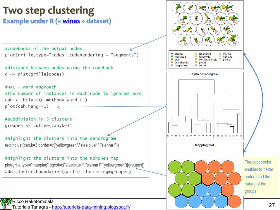
Two step clusteringExample under R (« wines » dataset)

#codebooks of the output nodes

plot(grille,type="codes",codeRendering = "segments")

#distance between nodes using the codebook

d <- dist(grille$codes)

#HAC – ward approach

#the number of instances in each node is ignored here

cah <- hclust(d,method="ward.D")

plot(cah,hang=-1)

#subdivision in 3 clusters

groupes <- cutree(cah,k=3)

#highlight the clusters into the dendrogram

rect.hclust(cah,k=3,border=c("yellowgreen","steelblue1","sienna1"))

#highlight the clusters into the Kohonen map

plot(grille,type="mapping",bgcol=c("steelblue1","sienna1","yellowgreen")[groupes])

add.cluster.boundaries(grille,clustering=groupes)

The codebooks

enables to better

understand the

nature of the

groups.


Ricco Rakotomalala


Assign a new instance to an existing cluster Proceed in two steps: identify the node of the

topological map associated to the new individual (See

Predicting the node membership of a new instance), and

then the cluster associated with this node.

Submit the new instant to the input layer, with

possibly the data transformation used during

the learning phase (standardization,...).

Identify the output neuron (winning neuron) in the

sense of the smallest distance to the codebook of

the neurons (e.g. Euclidean distance).

Identify the cluster (group) associated with the output-

layer neuron. The instance is assigned to this group.


Ricco Rakotomalala


Extension of SOM to the supervised learning task

Y = f(X1,X2, … ; α)


Ricco Rakotomalala


Supervised SOM

Solution 1. Construct the map in the (usual) unsupervised

fashion then, calculate the best prediction on each node

(the most common value of Y in the classification context,

average y in the regression context).

Solution 2. Add the information about the target attribute into the

codebooks. Calculate DX, distance to codebooks defined on the input

attributes; and DY distance defined on the target attribute.

Normalize DX and DY to balance their influences (i.e. define each D in

[0..1]), then calculate an overall distance that we can parameterize

D = α.DX + (1 – α).DY

We vary α according the relative

importance that we attach to X and Y


Ricco Rakotomalala


Conclusion

SOM serves both to the dimensionality reduction, data visualization and cluster

analysis (clustering).

The two-step approach for clustering is especially attractive.

This is a nonlinear approach for dimensionality reduction (vs. PCA for instance)

Numerous visualization possibilities

The method is simple, easy to explain ... and understand

Ability to handle large bases (linear complexity regarding the number of

observations and variables)

Pros

Cons

But ... the processing time may be long on very large bases (we need to pass

several times the individuals)

The visualization and the interpretation of codebooks becomes difficult

when the number of variables is very high


Ricco Rakotomalala


References

State-of-the art book

Kohonen T., « Self-Organizing Maps », 3rd Edition, Springer Series in Information Sciences, Vol. 30, 2001.

Course materials and tutorials

Ahn J.W., Syn S.Y., « Self Organizing Maps », 2005.

Bullinaria J.A., « Self Organizing Maps : Fundamentals », 2004.

Lynn Shane, « Self Organizing Maps for Customer Segmentation using R », R-bloggers, 2014.

Minsky M., « Kohonen’s Self Organizing Features Maps ».

Tanagra tutorial, « Self-organizing map (SOM) », July 2009.

Wikibooks – Data Mining Algorithms in R, « Clustering / Self Organizing Maps (SOM) ».

Scholarpedia, “Kohonen network”.


http://www.pitt.edu/~is2470pb/Spring05/FinalProjects/Group1a/tutorial/som.html

http://www.cs.bham.ac.uk/~jxb/NN/l16.pdf

http://www.r-bloggers.com/self-organising-maps-for-customer-segmentation-using-r/

http://www.ai-junkie.com/ann/som/som1.html

http://data-mining-tutorials.blogspot.fr/2009/07/self-organizing-map-som.html

https://en.wikibooks.org/wiki/Data_Mining_Algorithms_In_R/Clustering/Self-Organizing_Maps_(SOM)

http://www.scholarpedia.org/article/Kohonen_network

Data visualization, feature reduction and cluster...

Documents

Transcript of Data visualization, feature reduction and cluster...