Regression analysis with Python -...
20
Tanagra Data Mining Ricco Rakotomalala 9 octobre 2017 Page 1/20 1 Introduction Regression analysis with the StatsModels package for Python. Statsmodels is a Python module that provides classes and functions for the estimation of many different statistical models, as well as for conducting statistical tests, and statistical data exploration. The description of the library is available on the PyPI page, the repository that lists the tools and packages devoted to Python 1 . In this tutorial, we will try to identify the potentialities of StatsModels by conducting a case study in multiple linear regression. We will discuss about: the estimation of model parameters using the ordinary least squares method, the implementation of some statistical tests, the checking of the model assumptions by analyzing the residuals, the detection of 1 The French version of this tutorial was written in September 2015. We were using the version 0.6.1.
-
Upload
truongkhuong -
Category
Documents
-
view
243 -
download
3
Transcript of Regression analysis with Python -...
Tanagra Data Mining Ricco Rakotomalala
9 octobre 2017 Page 1/20
1 Introduction
Regression analysis with the StatsModels package for Python.
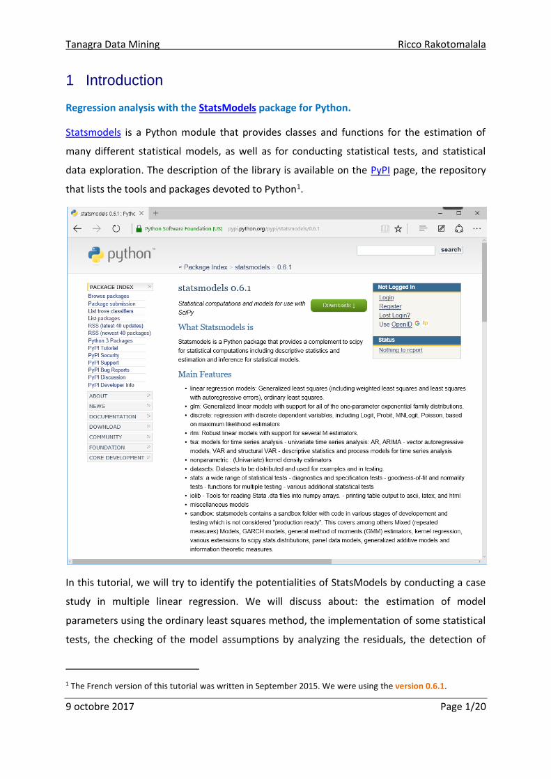
Statsmodels is a Python module that provides classes and functions for the estimation of
many different statistical models, as well as for conducting statistical tests, and statistical
data exploration. The description of the library is available on the PyPI page, the repository
that lists the tools and packages devoted to Python1.
In this tutorial, we will try to identify the potentialities of StatsModels by conducting a case
study in multiple linear regression. We will discuss about: the estimation of model
parameters using the ordinary least squares method, the implementation of some statistical
tests, the checking of the model assumptions by analyzing the residuals, the detection of
1 The French version of this tutorial was written in September 2015. We were using the version 0.6.1.

Tanagra Data Mining Ricco Rakotomalala
9 octobre 2017 Page 2/20
outliers and influential points, the analysis of multicollinearity, the calculation of the
prediction interval for a new instance.
About the regression analysis, an excellent reference is the online course available on the
PennState Eberly College of Science website: "STAT 501 - Regression Methods".
2 Dataset
We use the “vehicules_1.txt” data file for the construction of the model. It describes n = 26
vehicles from their characteristics: engine size (cylindrée), horsepower (puissance), weight
(poids) and consumption (conso, liter per 100 km).
modele cylindree puissance poids conso
Maserati Ghibli GT 2789 209 1485 14.5
Daihatsu Cuore 846 32 650 5.7
Toyota Corolla 1331 55 1010 7.1
Fort Escort 1.4i PT 1390 54 1110 8.6
Mazda Hachtback V 2497 122 1330 10.8
Volvo 960 Kombi aut 2473 125 1570 12.7
Toyota Previa salon 2438 97 1800 12.8
Renault Safrane 2.2. V 2165 101 1500 11.7
Honda Civic Joker 1.4 1396 66 1140 7.7
VW Golt 2.0 GTI 1984 85 1155 9.5
Suzuki Swift 1.0 GLS 993 39 790 5.8
Lancia K 3.0 LS 2958 150 1550 11.9
Mercedes S 600 5987 300 2250 18.7
Volvo 850 2.5 2435 106 1370 10.8
VW Polo 1.4 60 1390 44 955 6.5
Hyundai Sonata 3000 2972 107 1400 11.7
Opel Corsa 1.2i Eco 1195 33 895 6.8
Opel Astra 1.6i 16V 1597 74 1080 7.4
Peugeot 306 XS 108 1761 74 1100 9
Mitsubishi Galant 1998 66 1300 7.6
Citroen ZX Volcane 1998 89 1140 8.8
Peugeot 806 2.0 1998 89 1560 10.8
Fiat Panda Mambo L 899 29 730 6.1
Seat Alhambra 2.0 1984 85 1635 11.6
Ford Fiesta 1.2 Zetec 1242 55 940 6.6
We want to explain / predict the consumption of the cars (y : CONSO) from p = 3 input
(explanatory, predictor) variables (X1 : cylindrée, X2 : puissance, X3 : poids).
The regression equation is written as
nixaxaxaay iiiii ,,1,3322110
Tanagra Data Mining Ricco Rakotomalala
9 octobre 2017 Page 3/20
The aim of the regression analysis is to estimate the values of the coefficients (𝑎0, 𝑎1, 𝑎2, 𝑎3)
using the available dataset.
3 Data importation
We use the Pandas package for importing the data file into a data frame structure.
#modifying the default directory
import os
os.chdir("… directory containing the data file …")
#importing the Pandas library
#reading the data file with read.table()
import pandas
cars = pandas.read_table("vehicules_1.txt",sep="\t",header=0,index_col=0)
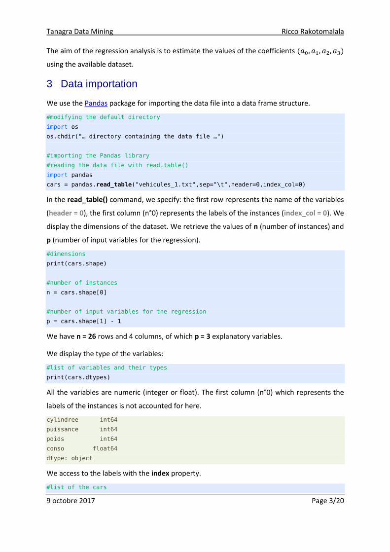
In the read_table() command, we specify: the first row represents the name of the variables
(header = 0), the first column (n°0) represents the labels of the instances (index_col = 0). We
display the dimensions of the dataset. We retrieve the values of n (number of instances) and
p (number of input variables for the regression).
#dimensions
print(cars.shape)
#number of instances
n = cars.shape[0]
#number of input variables for the regression
p = cars.shape[1] - 1
We have n = 26 rows and 4 columns, of which p = 3 explanatory variables.
We display the type of the variables:
#list of variables and their types
print(cars.dtypes)
All the variables are numeric (integer or float). The first column (n°0) which represents the
labels of the instances is not accounted for here.
cylindree int64
puissance int64
poids int64
conso float64
dtype: object
We access to the labels with the index property.
#list of the cars

Tanagra Data Mining Ricco Rakotomalala
9 octobre 2017 Page 4/20
print(cars.index)
We obtain:
Index(['Maserati Ghibli GT', 'Daihatsu Cuore', 'Toyota Corolla',
'Fort Escort 1.4i PT', 'Mazda Hachtback V', 'Volvo 960 Kombi aut',
'Toyota Previa salon', 'Renault Safrane 2.2. V',
'Honda Civic Joker 1.4', 'VW Golt 2.0 GTI', 'Suzuki Swift 1.0 GLS',
'Lancia K 3.0 LS', 'Mercedes S 600', 'Volvo 850 2.5', 'VW Polo 1.4 60',
'Hyundai Sonata 3000', 'Opel Corsa 1.2i Eco', 'Opel Astra 1.6i 16V',
'Peugeot 306 XS 108', 'Mitsubishi Galant', 'Citroen ZX Volcane',
'Peugeot 806 2.0', 'Fiat Panda Mambo L', 'Seat Alhambra 2.0',
'Ford Fiesta 1.2 Zetec'],
dtype='object', name='modele')
4 Regression analysis
4.1 Launching the analysis
We can perform the modelling step by importing the Statsmodels package. We have two
options. (1) The first consists of dividing the data into two parts: a vector containing the
values of the target variable CONSO, a matrix with the explanatory variables CYLINDREE,
POWER, CONSO. Then, we pass them to the OLS tool. This implies some manipulation of
data, and especially we must convert the data frame structure into numpy vector and
matrix. (2) The second is based on a specific tool (ols) which directly recognizes formulas
similar to the ones used under R [e. g. lm() function for R]. The Pandas data frame structure
can be used directly in this case. We prefer this second solution.
#regression with formula
import statsmodels.formula.api as smf
#instantiation
reg = smf.ols('conso ~ cylindree + puissance + poids', data = cars)
#members of reg object
print(dir(reg))
reg is an instance of the class ols. We can list their members with the dir() command i.e.
properties and methods.
['__class__', '__delattr__', '__dict__', '__dir__', '__doc__', '__eq__',
'__format__', '__ge__', '__getattribute__', '__gt__', '__hash__', '__init__',
'__le__', '__lt__', '__module__', '__ne__', '__new__', '__reduce__',
'__reduce_ex__', '__repr__', '__setattr__', '__sizeof__', '__str__',
'__subclasshook__', '__weakref__', '_data_attr', '_df_model', '_df_resid',
'_get_init_kwds', '_handle_data', '_init_keys', 'data', 'df_model', 'df_resid',
Tanagra Data Mining Ricco Rakotomalala
9 octobre 2017 Page 5/20
'endog', 'endog_names', 'exog', 'exog_names', 'fit', 'fit_regularized', 'formula',
'from_formula', 'hessian', 'information', 'initialize', 'k_constant', 'loglike',
'nobs', 'predict', 'rank', 'score', 'weights', 'wendog', 'wexog', 'whiten']
We use the fit() command to launch the modelling process on the dataset.
#launching the modelling process
res = reg.fit()
#members of the object provided by the modelling
print(dir(res))
The res object has also various properties and methods.
['HC0_se', 'HC1_se', 'HC2_se', 'HC3_se', '_HCCM', '__class__', '__delattr__',
'__dict__', '__dir__', '__doc__', '__eq__', '__format__', '__ge__',
'__getattribute__', '__gt__', '__hash__', '__init__', '__le__', '__lt__',
'__module__', '__ne__', '__new__', '__reduce__', '__reduce_ex__', '__repr__',
'__setattr__', '__sizeof__', '__str__', '__subclasshook__', '__weakref__',
'_cache', '_data_attr', '_get_robustcov_results', '_is_nested',
'_wexog_singular_values', 'aic', 'bic', 'bse', 'centered_tss', 'compare_f_test',
'compare_lm_test', 'compare_lr_test', 'condition_number', 'conf_int',
'conf_int_el', 'cov_HC0', 'cov_HC1', 'cov_HC2', 'cov_HC3', 'cov_kwds',
'cov_params', 'cov_type', 'df_model', 'df_resid', 'eigenvals', 'el_test', 'ess',
'f_pvalue', 'f_test', 'fittedvalues', 'fvalue', 'get_influence',
'get_robustcov_results', 'initialize', 'k_constant', 'llf', 'load', 'model',
'mse_model', 'mse_resid', 'mse_total', 'nobs', 'normalized_cov_params',
'outlier_test', 'params', 'predict', 'pvalues', 'remove_data', 'resid',
'resid_pearson', 'rsquared', 'rsquared_adj', 'save', 'scale', 'ssr', 'summary',
'summary2', 't_test', 'tvalues', 'uncentered_tss', 'use_t', 'wald_test', 'wresid']
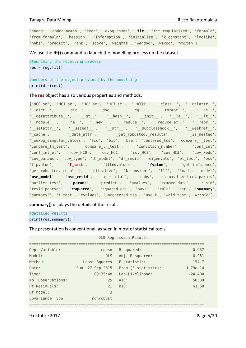
summary() displays the details of the result.
#detailed results
print(res.summary())
The presentation is conventional, as seen in most of statistical tools.
OLS Regression Results
==============================================================================
Dep. Variable: conso R-squared: 0.957
Model: OLS Adj. R-squared: 0.951
Method: Least Squares F-statistic: 154.7
Date: Sun, 27 Sep 2015 Prob (F-statistic): 1.79e-14
Time: 09:35:48 Log-Likelihood: -24.400
No. Observations: 25 AIC: 56.80
Df Residuals: 21 BIC: 61.68
Df Model: 3
Covariance Type: nonrobust
==============================================================================

Tanagra Data Mining Ricco Rakotomalala
9 octobre 2017 Page 6/20
coef std err t P>|t| [95.0% Conf. Int.]
------------------------------------------------------------------------------
Intercept 1.2998 0.614 2.117 0.046 0.023 2.577
cylindree -0.0005 0.000 -0.953 0.351 -0.002 0.001
puissance 0.0303 0.007 4.052 0.001 0.015 0.046
poids 0.0052 0.001 6.447 0.000 0.004 0.007
==============================================================================
Omnibus: 0.799 Durbin-Watson: 2.419
Prob(Omnibus): 0.671 Jarque-Bera (JB): 0.772
Skew: -0.369 Prob(JB): 0.680
Kurtosis: 2.558 Cond. No. 1.14e+04
==============================================================================
Warnings:
[1] Standard Errors assume that the covariance matrix of the errors is correctly
specified.
[2] The condition number is large, 1.14e+04. This might indicate that there are
strong multicollinearity or other numerical problems.
The coefficient of determination is equal to R² = 0.975. The regression is globally significant
at the 5% level [F-statistic = 154.7, with Prob(F-statistic) = 1.79e-14]. All the coefficients
seem also significant at the 5% level (see t and P>|t| into the coefficients table).
Everything seems to be going well. But a warning message alerts us nevertheless. A
collinearity problem between explanatory variables is suspected. We will check it later.
4.2 Intermediate computations
The object res enables to perform intermediate calculations. Some are relatively simple.
Below, we display some important results (estimated coefficients, R2). We try to calculate
manually the F-Statistic. We have the same as the value provided by the res object of course.
#estimated coefficients
print(res.params)
#R2
print(res.rsquared)
#calculating the F-statistic
F = res.mse_model / res.mse_resid
print(F)
#F provided by the res object
print(res.fvalue)

Tanagra Data Mining Ricco Rakotomalala
9 octobre 2017 Page 7/20
Other calculations are possible, giving us access to sophisticated procedures such as tests
that a subset of the slopes is null.
We try to test that all the slopes are 0. This is a special case of the testing that a subset is
null. The null hypothesis may be written in a matrix format.
0:0 RaH
Where
• a = (a0,a1,a2,a3) is the vector of the coefficients;
• R is the matrix of constraints:
1000
0100
0010
R
We can write the test in a more explicit form:
0
0
0
:
0
0
0
1000
0100
0010
:
3
2
1
0
3
2
1
0
0
a
a
a
H
a
a
a
a
H
In Python, we describe the R matrix, then we call the f_test() procedure:
#test for a linear combination of coefficients
#all the slopes are zero
import numpy as np
#matrix R
R = np.array([[0,1,0,0],[0,0,1,0],[0,0,0,1]])
#F-statistic
print(res.f_test(R))
We obtain the F-statistic for the global significance (model significance).
<F test: F=array([[ 154.67525358]]), p=1.7868899968536844e-14, df_denom=21, df_num=3>

Tanagra Data Mining Ricco Rakotomalala
9 octobre 2017 Page 8/20
5 Regression diagnostic
5.1 Model assumptions – Test for error normality
One of the main assumption for the inferential part of the regression (OLS - ordinary least
squares) is the assumption that the errors follow a normal distribution. A first important
verification is to check the compatibility of the residuals (the errors observed on the sample)
with this assumption.
Jarque-Bera Test. We use the stattools module in order to perform the Jarque-Bera test.
This test checks if the observed skewness and kurtosis matching a normal distribution.
#Jarque-Bera normality test
import statsmodels.api as sm
JB, JBpv,skw,kurt = sm.stats.stattools.jarque_bera(res.resid)
print(JB,JBpv,skw,kurt)
We have respectively: the statistic JB, the p-value of the test JBpv, the skewness skw and the
kurtosis kurt.
0.7721503004927122 0.679719442677 -0.3693040742424057 2.5575948785729956
We observe that the values obtained (JB, JBpv) are consistent with those provided by the
summary() command above (page 5). Here, we can assume that the errors are a normal
distribution at the 5% level.
Normal probability plot. The normal probability plot is a graphical technique to identify
substantive departures from normality. It is based on the comparison between the observed
distribution and the theoretical distribution under the normal assumption. The null
hypothesis (normal distribution) is rejected if the points are not aligned on a straight line.
We use the qqplot() procedure.
#qqpolot vs. normal distribution
sm.qqplot(res.resid)
We have a graphical representation.

Tanagra Data Mining Ricco Rakotomalala
9 octobre 2017 Page 9/20
The graph confirms the Jarque-Bera test. The points are approximately aligned. But there
seems to be some problems with the high values of the residuals. This suggests the existence
of atypical points in our data.
5.2 Detection of outliers and influential points
We use a specific object provided by the regression result to analyze the influential points.
#object for the analysis of influential points
infl = res.get_influence()
#members
print(dir(infl))
We have some properties and methods.
['__class__', '__delattr__', '__dict__', '__dir__', '__doc__', '__eq__',
'__format__', '__ge__', '__getattribute__', '__gt__', '__hash__', '__init__',
'__le__', '__lt__', '__module__', '__ne__', '__new__', '__reduce__',
'__reduce_ex__', '__repr__', '__setattr__', '__sizeof__', '__str__',
'__subclasshook__', '__weakref__', '_get_drop_vari', '_ols_xnoti', '_res_looo',
'aux_regression_endog', 'aux_regression_exog', 'cooks_distance', 'cov_ratio',
'det_cov_params_not_obsi', 'dfbetas', 'dffits', 'dffits_internal', 'endog',
'ess_press', 'exog', 'get_resid_studentized_external', 'hat_diag_factor',
'hat_matrix_diag', 'influence', 'k_vars', 'model_class', 'nobs', 'params_not_obsi',
'resid_press', 'resid_std', 'resid_studentized_external',
'resid_studentized_internal', 'resid_var', 'results', 'sigma2_not_obsi',
'sigma_est', 'summary_frame', 'summary_table']
Leverage and internally studentized residuals (standardized residuals). We display for
instance the leverage and the internally studentized residuals.
#leverage
print(infl.hat_matrix_diag)

Tanagra Data Mining Ricco Rakotomalala
9 octobre 2017 Page 10/20
#internally studentized residuals
print(infl.resid_studentized_internal)
We have, respectively: leverage,
[ 0.72183931 0.17493953 0.06052439 0.05984303 0.05833457 0.09834565
0.3069384 0.09434881 0.07277269 0.05243782 0.11234304 0.08071319
0.72325833 0.05315383 0.08893405 0.25018637 0.10112179 0.0540076
0.05121573 0.10772156 0.05567033 0.16884879 0.13204031 0.24442832
0.07603257]
and internally studentized residuals.
[ 1.27808674 0.70998577 -0.71688165 0.81147383 0.10804304 0.93643923
0.61326258 0.85119912 -1.28230456 0.82173104 -0.4825047 -0.89285915
-1.47915409 0.46985347 -0.65771702 2.12388261 0.62133156 -1.46735362
0.84071707 -2.28450314 -0.25846374 -0.56426915 0.84517318 0.26915841
-0.98733251]
Knowing how to code allows us to verify by calculation the results proposed by the different
procedures. For instance, we can obtain the internally studentized residuals (ti) from the
residuals iii yy ˆˆ , the leverage ih and the regression standard error ̂ obtained from
the scale property of the object resulting from the regression (res.scale):
i
ii
ht
1ˆ
ˆ
We use the following commands:
#checking the values of the internally studentized residuals
import numpy as np
residus = res.resid.as_matrix() #residuals
leviers = infl.hat_matrix_diag #leverage
sigma_err = np.sqrt(res.scale) #regression standard error
res_stds = residus/(sigma_err*np.sqrt(1.0-leviers))
print(res_stds)
The values are consistent to those provided directly with the property
"resid_studenized_internal". Fortunately, we would have been quite disturbed otherwise.
Externally studentized residuals. We repeat the approach for the externally studentized
residuals, using the following formula:
2
*
1
2
i
iitpn
pntt
Tanagra Data Mining Ricco Rakotomalala
9 octobre 2017 Page 11/20
We compare the values provided by the property resid_studentized_external and the values
obtained by the formula above.
#values provided by the property of the object
print(infl.resid_studentized_external)
#checking with the formula
res_studs = res_stds*np.sqrt((n-p-2)/(n-p-1-res_stds**2))
print(res_studs)
Here also, the results are consistent.
[ 1.29882255 0.70134375 -0.70832574 0.80463315 0.10546853 0.933571
0.60391521 0.8453972 -1.30347228 0.81513961 -0.4735084 -0.88836644
-1.52514011 0.46095935 -0.64858111 2.33908893 0.61200904 -1.51157649
0.83462166 -2.57180996 -0.25263694 -0.55489299 0.83920081 0.26312597
-0.98671171]
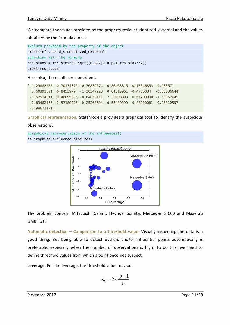
Graphical representation. StatsModels provides a graphical tool to identify the suspicious
observations.
#graphical representation of the influences()
sm.graphics.influence_plot(res)
The problem concern Mitsubishi Galant, Hyundai Sonata, Mercedes S 600 and Maserati
Ghibli GT.
Automatic detection – Comparison to a threshold value. Visually inspecting the data is a
good thing. But being able to detect outliers and/or influential points automatically is
preferable, especially when the number of observations is high. To do this, we need to
define threshold values from which a point becomes suspect.
Leverage. For the leverage, the threshold value may be:
n
psh
12

Tanagra Data Mining Ricco Rakotomalala
9 octobre 2017 Page 12/20
An observation is suspicious if hi sh
#threshold leverage
seuil_levier = 2*(p+1)/n
print(seuil_levier)
#identification
atyp_levier = leviers > seuil_levier
print(atyp_levier)
Python displays a vector of Boolean values. True represents instances with a leverage higher
than the threshold value.
[ True False False False False False False False False False False False
True False False False False False False False False False False False False]
The reading is not easy. It is more convenient to display the index of the vehicles.
#which vehicles?
print(cars.index[atyp_levier],leviers[atyp_levier])
We have both the car model and the values of the leverage.
Index(['Maserati Ghibli GT', 'Mercedes S 600'], dtype='object', name='modele') [
0.72183931 0.72325833]
Externally studentized residuals. The probability distribution of the externally studentized
residuals is a Student distribution with (n-p-2) degrees of freedom. Thus, at the 5% level, the
threshold value is
)2(2
05.01
pntst
Where t1-0.05/2 is the quantile of the t distribution for a probability 0.975.
An observation is suspicious if
ti st *
#threshold externally studentized residuals
import scipy
seuil_stud = scipy.stats.t.ppf(0.975,df=n-p-2)
print(seuil_stud)
#detection - absolute value > threshold
atyp_stud = np.abs(res_studs) > seuil_stud
#which ones?
print(cars.index[atyp_stud],res_studs[atyp_stud])

Tanagra Data Mining Ricco Rakotomalala
9 octobre 2017 Page 13/20
These are,
Index(['Hyundai Sonata 3000', 'Mitsubishi Galant'], dtype='object', name='modele')
[ 2.33908893 -2.57180996]
Combination of leverage and externally studentized residuals. By combining the two
approaches with the logical operator OR,
#suspicious observations with one of the two criteria
pbm_infl = np.logical_or(atyp_levier,atyp_stud)
print(cars.index[pbm_infl]))
We identify 4 vehicles which are highlighted into the graphical representation above.
Index(['Maserati Ghibli GT', 'Mercedes S 600', 'Hyundai Sonata 3000',
'Mitsubishi Galant'], dtype='object', name='modele')
Other criteria. The tool provides other criteria such as DFFITS, Cook’s distance, etc. We can
present them in a tabular form.
#Other criteria for detecting influential points
print(infl.summary_frame().filter(["hat_diag","student_resid","dffits","cooks_d"]))
Values should be compared with their respective thresholds:
• n
pDFFITSi
12
for DFFITS ;
• 1
4
pnDi for Cook’s distance.
hat_diag student_resid dffits cooks_d
modele
Maserati Ghibli GT 0.721839 1.298823 2.092292 1.059755
Daihatsu Cuore 0.174940 0.701344 0.322948 0.026720
Toyota Corolla 0.060524 -0.708326 -0.179786 0.008277
Fort Escort 1.4i PT 0.059843 0.804633 0.203004 0.010479
Mazda Hachtback V 0.058335 0.105469 0.026251 0.000181
Volvo 960 Kombi aut 0.098346 0.933571 0.308322 0.023912
Toyota Previa salon 0.306938 0.603915 0.401898 0.041640
Renault Safrane 2.2. V 0.094349 0.845397 0.272865 0.018870
Honda Civic Joker 1.4 0.072773 -1.303472 -0.365168 0.032263
VW Golt 2.0 GTI 0.052438 0.815140 0.191757 0.009342
Suzuki Swift 1.0 GLS 0.112343 -0.473508 -0.168453 0.007366
Lancia K 3.0 LS 0.080713 -0.888366 -0.263232 0.017498
Mercedes S 600 0.723258 -1.525140 -2.465581 1.429505
Volvo 850 2.5 0.053154 0.460959 0.109217 0.003098
VW Polo 1.4 60 0.088934 -0.648581 -0.202639 0.010557
Hyundai Sonata 3000 0.250186 2.339089 1.351145 0.376280
Tanagra Data Mining Ricco Rakotomalala
9 octobre 2017 Page 14/20
Opel Corsa 1.2i Eco 0.101122 0.612009 0.205272 0.010858
Opel Astra 1.6i 16V 0.054008 -1.511576 -0.361172 0.030731
Peugeot 306 XS 108 0.051216 0.834622 0.193913 0.009538
Mitsubishi Galant 0.107722 -2.571810 -0.893593 0.157516
Citroen ZX Volcane 0.055670 -0.252637 -0.061340 0.000985
Peugeot 806 2.0 0.168849 -0.554893 -0.250103 0.016171
Fiat Panda Mambo L 0.132040 0.839201 0.327318 0.027167
Seat Alhambra 2.0 0.244428 0.263126 0.149659 0.005859
Ford Fiesta 1.2 Zetec 0.076033 -0.986712 -0.283049 0.020054
Note: Detecting outliers or influential points is one thing, dealing them is another. Indeed,
we cannot remove them systematically. It is necessary to identify why an observation is
problematic and thus to determine the most appropriate solution, which may be deletion,
but not systematically. For instance, let us take a simple situation. A point can be atypical
because it takes an unusual value on a variable. If the variable selection process leads to its
exclusion from the model, what should be done then? Re-enter the point? Leave as is? There
is no pre-determined solution. The modelling process is exploratory in nature.
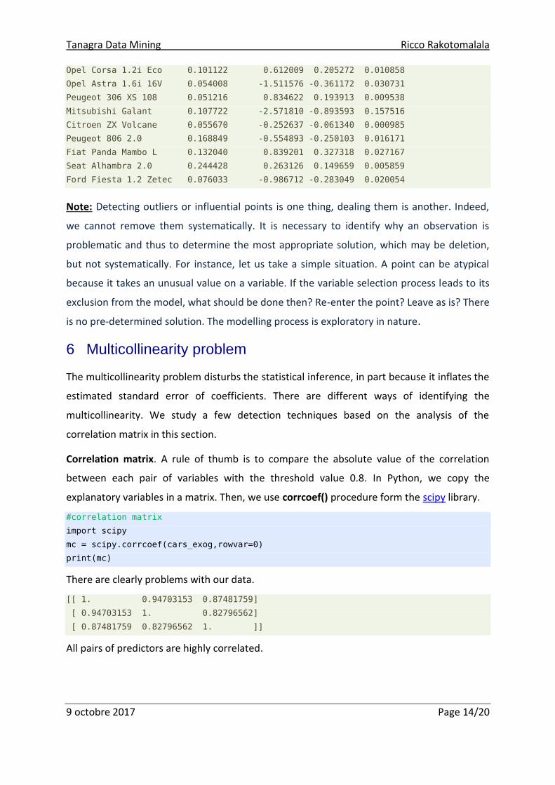
6 Multicollinearity problem
The multicollinearity problem disturbs the statistical inference, in part because it inflates the
estimated standard error of coefficients. There are different ways of identifying the
multicollinearity. We study a few detection techniques based on the analysis of the
correlation matrix in this section.
Correlation matrix. A rule of thumb is to compare the absolute value of the correlation
between each pair of variables with the threshold value 0.8. In Python, we copy the
explanatory variables in a matrix. Then, we use corrcoef() procedure form the scipy library.
#correlation matrix
import scipy
mc = scipy.corrcoef(cars_exog,rowvar=0)
print(mc)
There are clearly problems with our data.
[[ 1. 0.94703153 0.87481759]
[ 0.94703153 1. 0.82796562]
[ 0.87481759 0.82796562 1. ]]
All pairs of predictors are highly correlated.

Tanagra Data Mining Ricco Rakotomalala
9 octobre 2017 Page 15/20
Klein’s rule of thumb. It consists in comparing the square of the correlation between the
pairs of predictors with the overall R2 (R² = 0.957) of the regression. It is interesting because
it takes into account the characteristics of the regression.
#Klein’s rule of thumb
mc2 = mc**2
print(mc2)
None of the values exceed the R², but there are uncomfortable similarities nonetheless.
[[ 1. 0.89686872 0.76530582]
[ 0.89686872 1. 0.68552706]
[ 0.76530582 0.68552706 1. ]]
Variance Inflation Factor (VIF). This criterion makes it possible to evaluate the relationship
of one predictor with all other explanatory variables. We can read its value on the diagonal
of the inverse of the correlation matrix.
#VIF criterion
vif = np.linalg.inv(mc)
print(vif)
A possible rule for multicollinearity detection is (VIF > 4). Here also, we note that the
multicollinearity problem affects our regression.
[[ 12.992577 -9.20146328 -3.7476397 ]
[ -9.20146328 9.6964853 0.02124552]
[ -3.7476397 0.02124552 4.26091058]]
Possible solutions. Regularized least squares or variable selection approaches are possible
solution for the multicollinearity problem. It seems that they are not available in the
Statsmodels package. But it is not matter , Python is a powerful programming language, it
would be easy for us to program additional calculations from the objects provided by
Statsmodels.
7 Prediction and prediction interval
Applying the model on unseen instances (instances for which only the values of the
explanatory variables are available) to obtain the expected values of the target variable is
one of the objectives of the regression. The prediction is all the more credible if we can
provide a prediction interval with a certain probability (confidence level) of containing the
true value of the target variable.

Tanagra Data Mining Ricco Rakotomalala
9 octobre 2017 Page 16/20
In our case, this is above all an exercise. We apply the model on a set of observations not
used during the modelling process. We therefore have the values of both predictors and
target variable. This would allow us to verify the reliability of our model by comparing
predicted and observed values. It is a kind of holdout validation scheme. This approach is
widely use in classification problems.
7.1 Data importation
Here is the “vehicules_2.txt” data file:
modele cylindree puissance poids conso
Nissan Primera 2.0 1997 92 1240 9.2
Fiat Tempra 1.6 Liberty 1580 65 1080 9.3
Opel Omega 2.5i V6 2496 125 1670 11.3
Subaru Vivio 4WD 658 32 740 6.8
Seat Ibiza 2.0 GTI 1983 85 1075 9.5
Ferrari 456 GT 5474 325 1690 21.3
For these n*=6 vehicles, we calculate the prediction and we compare them to the observed
values of the target attribute.
We load the data file in a new data frame cars2.
#loading the second data file
cars2 = pandas.read_table("vehicules_2.txt",sep="\t",header=0,index_col=0)
#number of instances
n_pred = cars2.shape[0]
#description of the new cars
print(cars2)
The structure of the data file (index, columns) is identical to the first dataset.
cylindree puissance poids conso
modele
Nissan Primera 2.0 1997 92 1240 9.2
Fiat Tempra 1.6 Liberty 1580 65 1080 9.3
Opel Omega 2.5i V6 2496 125 1670 11.3
Subaru Vivio 4WD 658 32 740 6.8
Seat Ibiza 2.0 GTI 1983 85 1075 9.5
Ferrari 456 GT 5474 325 1690 21.3

Tanagra Data Mining Ricco Rakotomalala
9 octobre 2017 Page 17/20
7.2 Punctual prediction
The predicted value of the response is obtained by applying the model on the predictor
values. Using the matrix form is better when the number of instances to process is high:
aXy ˆ**
Where â is the vector of estimated coefficients, including the intercept. So that the
calculation is consistent, we must add to the X* matrix a column of 1. The dimension of the
matrix X* is (n*, p+1).
In Python, we create the matrix with the new column, we use the add_constant() procedure.
#predictor columns
cars2_exog = cars2[['cylindree','puissance','poids']]
#add a column of 1
cars2_exog = sm.add_constant(cars2_exog)
print(cars2_exog)
The constant value 1 is in the first column. The target variable CONSO is not included in the
X* matrix of course.
const cylindree puissance poids
modele
Nissan Primera 2.0 1 1997 92 1240
Fiat Tempra 1.6 Liberty 1 1580 65 1080
Opel Omega 2.5i V6 1 2496 125 1670
Subaru Vivio 4WD 1 658 32 740
Seat Ibiza 2.0 GTI 1 1983 85 1075
Ferrari 456 GT 1 5474 325 1690
Then, we apply the coefficients of the regression with the predict() command…
#punctual prediction by applying the regression coefficients
pred_conso = reg.predict(res.params,cars2_exog)
print(pred_conso)
… to obtain the predicted values.
[ 9.58736855 8.1355859 12.58619059 5.80536066 8.52394228 17.33247145]
7.3 Comparison of predicted values and observed values
A scatterplot enables to check the quality of prediction. We set in the x axis the observed
values of the response variable, in the y axis the predicted values. If the prediction is perfect,
the plotted points are aligned in the diagonal. We use the matplotlib package for Python.
#comparison obs. Vs. pred.
import matplotlib.pyplot as plt

Tanagra Data Mining Ricco Rakotomalala
9 octobre 2017 Page 18/20
plt.scatter(cars2['conso'],pred_conso)
plt.plot(np.arange(5,23),np.arange(5,23))
plt.xlabel('Valeurs Observées')
plt.ylabel('Valeurs Prédites')
plt.xlim(5,22)
plt.ylim(5,22)
plt.show()
The prediction is acceptable for 5 points. For the 6th, the Ferrari, the regression model
strongly underestimates the consumption (17.33 vs. 21.3).
7.4 Prediction interval
A punctual prediction is a first step. A prediction interval is always more interesting because
we can associate a probability of error to the result provided.
Standard error of the prediction. The calculation is quite complex. We need to calculate the
standard error of the prediction for each individual, we use the following formula (squared
value of the standard error of the prediction) for a new instance i*
*
1
*
22ˆ ''1ˆˆ
* ii XXXXi
Some information is provided by the Python objects reg and res (sections 4.1 and Erreur ! S
ource du renvoi introuvable.) : 2ˆ is the square of the residual standard error, 1
'
XX is
obtained from the matrix of explanatory variables. Other information is related to the new
individual: *iX is the values of the input attributes, including the constant 1. For instance,
for (Nissan Primera 2.0), we have the vector (1 ; 1997 ; 92 ; 1240).
Let us see how to organize this in a Python program.

Tanagra Data Mining Ricco Rakotomalala
9 octobre 2017 Page 19/20
#retrieving the matrix (X'X)-1
inv_xtx = reg.normalized_cov_params
print(inv_xtx)
#description of the new instances: transformation in matrix
X_pred = cars2_exog.as_matrix()
#### squared value of the standard error of the prediction ###
#initialization
var_err = np.zeros((n_pred,))
#for each individual to process
for i in range(n_pred):
#description of the individual
tmp = X_pred[i,:]
#matrix product
pm = np.dot(np.dot(tmp,inv_xtx),np.transpose(tmp))
#squared values
var_err[i] = res.scale * (1 + pm)
#
print(var_err)
We obtain:
[ 0.51089413 0.51560511 0.56515759 0.56494062 0.53000431 1.11282003]
Confidence interval. Now we calculate the lower and upper bounds for a 95% confidence
level, using the quantile of the Student distribution and the punctual prediction.
#quantile of the Student distribution (0.975)
qt = scipy.stats.t.ppf(0.975,df=n-p-1)
#lower bound
yb = pred_conso - qt * np.sqrt(var_err)
print(yb)
#upper bound
yh = pred_conso + qt * np.sqrt(var_err)
print(yh)
For the 6 cars of the second data file, we obtain:
[ 8.1009259 6.6423057 11.02280004 4.24227024 7.00995439 15.13868086]
[ 11.07381119 9.62886611 14.14958114 7.36845108 10.03793016 19.52626203]
Checking of the prediction interval. The evaluation takes on a concrete dimension here
since we check, for a given confidence level, if the confidence interval contains the true
(observed) value of the response variable. We organize the presentation in such a way that
the observed values are surrounded by the lower and upper bounds of the intervals.

Tanagra Data Mining Ricco Rakotomalala
9 octobre 2017 Page 20/20
#matrix with the various values (lower bound, observed, upper bound)
a = np.resize(yb,new_shape=(n_pred,1))
y_obs = cars2['conso']
a = np.append(a,np.resize(y_obs,new_shape=(n_pred,1)),axis=1)
a = np.append(a,np.resize(yh,new_shape=(n_pred,1)),axis=1)
#transforming in a data frame object to obtain better displaying
df = pandas.DataFrame(a)
df.index = cars2.index
df.columns = ['B.Basse','Y.Obs','B.Haute']
print(df)
It is confirmed, the Ferrari is crossing the limits (if I may say so).
B.Basse Y.Obs B.Haute
modele
Nissan Primera 2.0 8.100926 9.2 11.073811
Fiat Tempra 1.6 Liberty 6.642306 9.3 9.628866
Opel Omega 2.5i V6 11.022800 11.3 14.149581
Subaru Vivio 4WD 4.242270 6.8 7.368451
Seat Ibiza 2.0 GTI 7.009954 9.5 10.037930
Ferrari 456 GT 15.138681 21.3 19.526262
8 Conclusion
The StatsModels package provides interesting features for statistical modeling. Coupled with
the Python language and other packages (numpy, scipy, pandas, etc.), the possibilities
become immense. The skills that we have been able to develop under R are very easy to
transpose here.