Tanagra Kohonen SOM -...

Didacticiel - Études de cas R.R.

1er juillet 2009 sur 14

1 Subject Implementing the Kohonen’s SOM (Self Organizing Map) algorithm with Tanagra.

A self-organizing map (SOM) or self-organizing feature map (SOFM) is a kind of artificial neural

network that is trained using unsupervised learning to produce a low-dimensional (typically two-

dimensional), discretized representation of the input space of the training samples, called a map.

Self-organizing maps are different than other artificial neural networks in the sense that they use a

neighborhood function to preserve the topological properties of the input space

(http://en.wikipedia.org/wiki/Self-organizing_map).

SOM is a clustering method. Indeed, it organizes the data in clusters (cells of map) such as the

instances in the same cell are similar, and the instances in different cells are different. In this point

of view, SOM gives comparable results to state-of-the-art clustering algorithm such as K-Means

(Forgy, 1965; McQueen, 1967).

SOM can be viewed also as a visualization technique. It allows us to visualize in a low dimensional

representation space (2D) the original dataset. Indeed, the individuals located in adjacent cells are

more similar than individuals located in distant cells. In this point of view, it is comparable to

visualization techniques such as Multidimensional scaling (Kruskal, 1978) or PCA (Principal

Component Analysis, http://en.wikipedia.org/wiki/Principal_component_analysis).

In this tutorial, we show how to implement the Kohonen's SOM algorithm with Tanagra. We try to

assess the properties of this approach by comparing the results with those of the PCA algorithm.

Then, we compare the results to those of K-Means, which is a clustering algorithm. Finally, we

implement the Two-step Clustering process by combining the SOM algorithm with the HAC

process (Hierarchical Agglomerative Clustering). It is a variant of the Two-Step Clustering where

we combine K-Means and HAC (http://data-mining-tutorials.blogspot.com/2009/06/two-step-

clustering-for-handling-large.html). We observe that the HAC primarily merges the adjacent cells.

2 Dataset We analyze the WAVEFORM dataset (Breiman and al., 1984)1. This is an artificial dataset2.

There are 21 descriptors. We have 5000 instances. We do not use the CLASS attribute which

classify the instances into 3 pre-defined classes in this tutorial.

1 http://eric.univ‐lyon2.fr/~ricco/tanagra/fichiers/waveform_unsupervised.xls

2 http://archive.ics.uci.edu/ml/datasets/Waveform+Database+Generator+%28Version+1%29



3 Kohonen’s SOM approach with Tanagra

3.1 Importing the data file

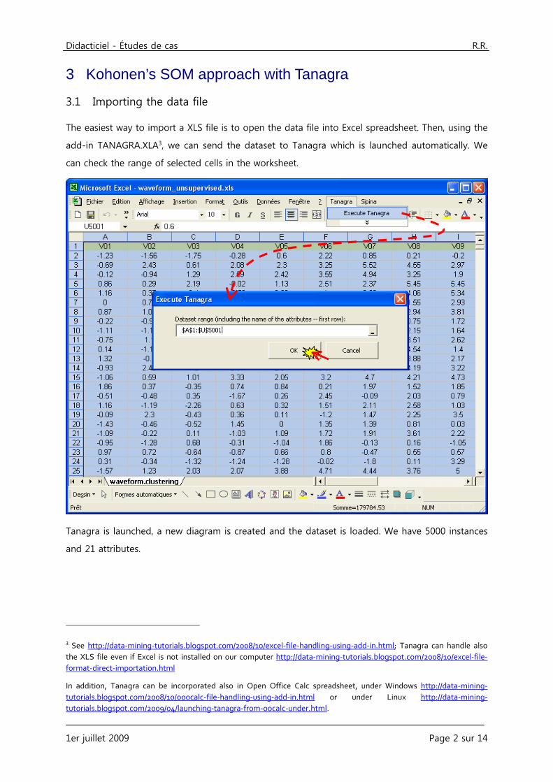
The easiest way to import a XLS file is to open the data file into Excel spreadsheet. Then, using the

add-in TANAGRA.XLA3, we can send the dataset to Tanagra which is launched automatically. We

can check the range of selected cells in the worksheet.

Tanagra is launched, a new diagram is created and the dataset is loaded. We have 5000 instances

and 21 attributes.

3 See http://data‐mining‐tutorials.blogspot.com/2008/10/excel‐file‐handling‐using‐add‐in.html; Tanagra can handle also the XLS file even if Excel is not installed on our computer http://data‐mining‐tutorials.blogspot.com/2008/10/excel‐file‐format‐direct‐importation.html

In addition, Tanagra can be incorporated also in Open Office Calc spreadsheet, under Windows http://data‐mining‐tutorials.blogspot.com/2008/10/ooocalc‐file‐handling‐using‐add‐in.html or under Linux http://data‐mining‐tutorials.blogspot.com/2009/04/launching‐tanagra‐from‐oocalc‐under.html.



3.2 Descriptive statistics and outliers detection

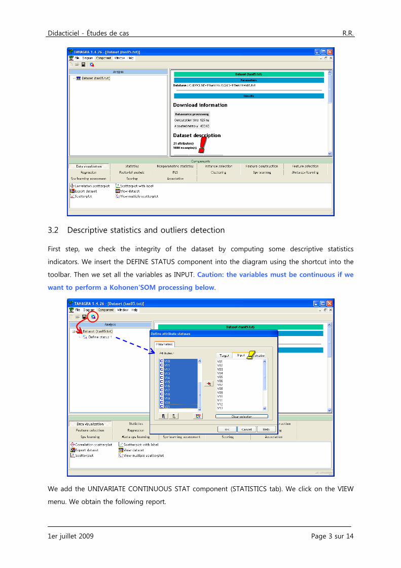
First step, we check the integrity of the dataset by computing some descriptive statistics

indicators. We insert the DEFINE STATUS component into the diagram using the shortcut into the

toolbar. Then we set all the variables as INPUT. Caution: the variables must be continuous if we

want to perform a Kohonen'SOM processing below.

We add the UNIVARIATE CONTINUOUS STAT component (STATISTICS tab). We click on the VIEW

menu. We obtain the following report.



We note that there is no constant in our dataset i.e. standard deviation = 0. We note also that all

the variables seem defined in the same scale.

We can complete this dataset checkout by detecting eventual outliers. We add the UNIVARIATE

OUTLIER DETECTION (STATISTICS tab) component4.

4 See http://data‐mining‐tutorials.blogspot.com/2009/06/univariate‐outlier‐detection‐methods.html



Whatever the variable, there is no unusual value. It is not surprising. We know that this dataset is

generated artificially.

3.3 The KOHONEN-SOM component

We want to launch the analysis now. We create a grid with 2 rows and 3 columns i.e. a

classification of the instances into 6 groups (2 x 3 = 6 clusters).

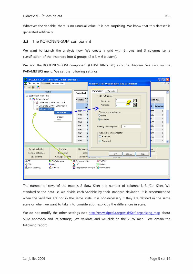
We add the KOHONEN-SOM component (CLUSTERING tab) into the diagram. We click on the

PARAMETERS menu. We set the following settings.

The number of rows of the map is 2 (Row Size), the number of columns is 3 (Col Size). We

standardize the data i.e. we divide each variable by their standard deviation. It is recommended

when the variables are not in the same scale. It is not necessary if they are defined in the same

scale or when we want to take into consideration explicitly the differences in scale.

We do not modify the other settings (see http://en.wikipedia.org/wiki/Self-organizing_map about

SOM approach and its settings). We validate and we click on the VIEW menu. We obtain the

following report.



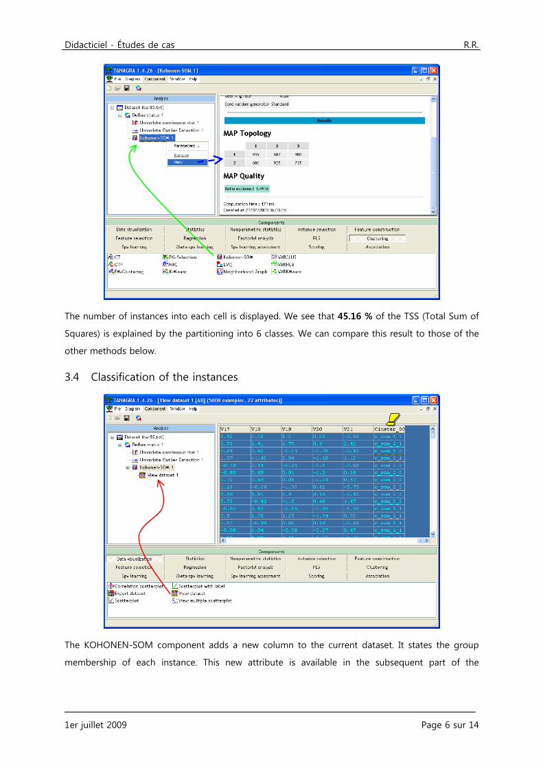
The number of instances into each cell is displayed. We see that 45.16 % of the TSS (Total Sum of

Squares) is explained by the partitioning into 6 classes. We can compare this result to those of the

other methods below.

3.4 Classification of the instances

The KOHONEN-SOM component adds a new column to the current dataset. It states the group

membership of each instance. This new attribute is available in the subsequent part of the



diagram. We can visualize the current dataset with the VIEW DATASET component. We see for

instance that the first example belongs to the cell (1, 3) i.e. first row and third column.

Note: we can classify an additional instance with the same framework i.e. an example which is not

involved in the learning process. This deployment phase is one of the most important steps of the

Data Mining process5.

4 Proximity of nodes into the grid Individuals who are in adjacent cells are also close in the original representation space. This is one

of the main interests of this method. Let us check this assertion on the WAVEFORM dataset.

We cannot visualize the dataset into the original space. So we use a PCA in order to obtain a 2D

representation. We try to visualize the relative positions of groups (clusters) in the scatter plot.

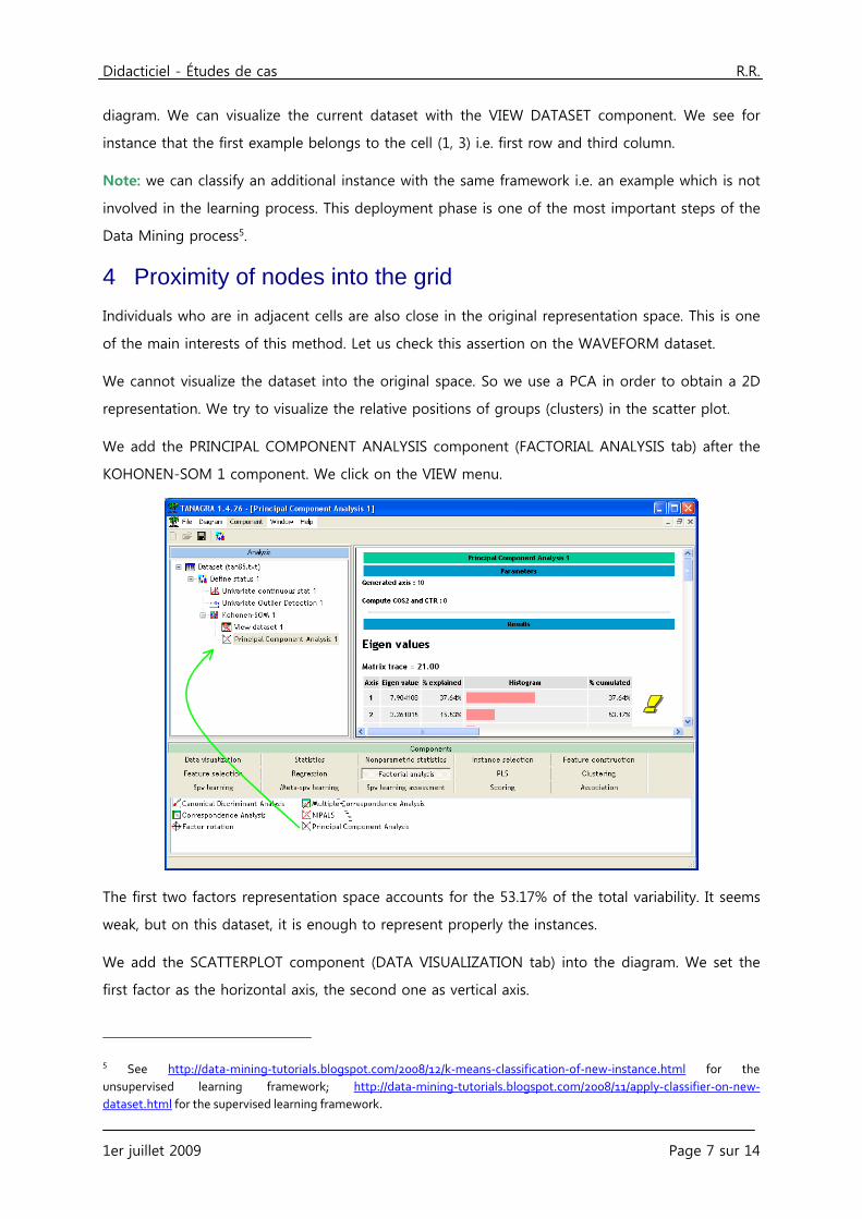
We add the PRINCIPAL COMPONENT ANALYSIS component (FACTORIAL ANALYSIS tab) after the

KOHONEN-SOM 1 component. We click on the VIEW menu.

The first two factors representation space accounts for the 53.17% of the total variability. It seems

weak, but on this dataset, it is enough to represent properly the instances.

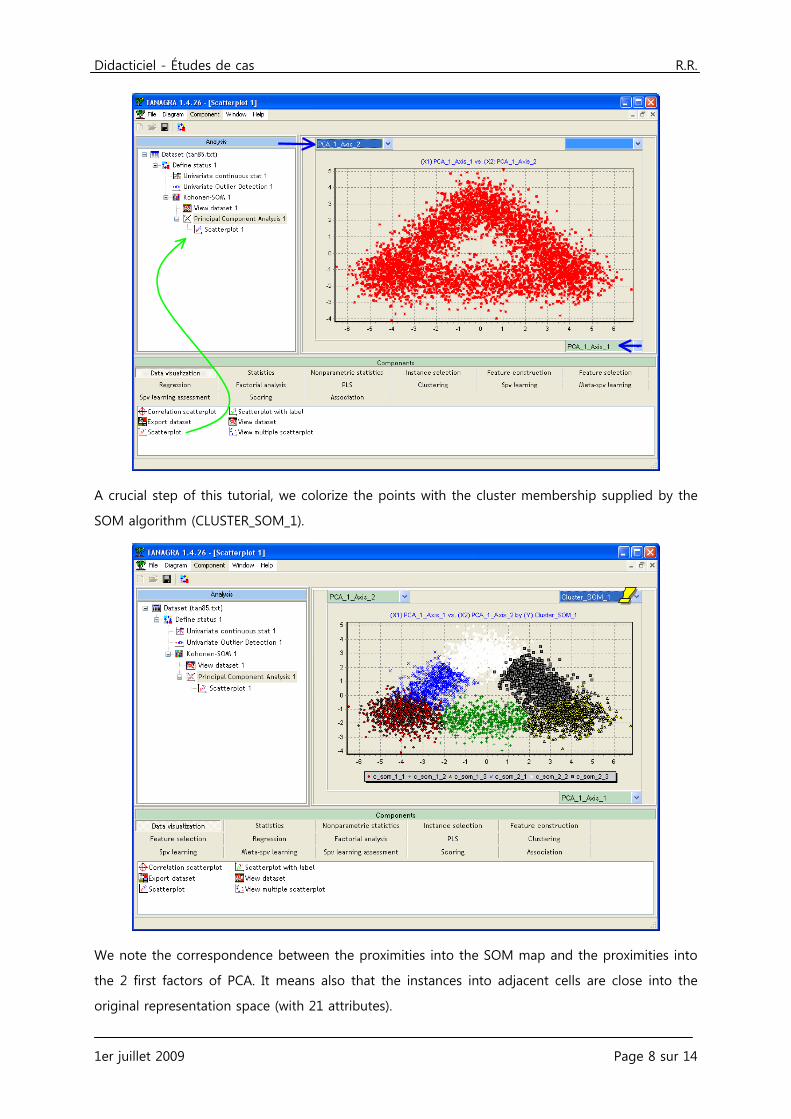
We add the SCATTERPLOT component (DATA VISUALIZATION tab) into the diagram. We set the

first factor as the horizontal axis, the second one as vertical axis.

5 See http://data‐mining‐tutorials.blogspot.com/2008/12/k‐means‐classification‐of‐new‐instance.html for the unsupervised learning framework; http://data‐mining‐tutorials.blogspot.com/2008/11/apply‐classifier‐on‐new‐dataset.html for the supervised learning framework.



A crucial step of this tutorial, we colorize the points with the cluster membership supplied by the

SOM algorithm (CLUSTER_SOM_1).

We note the correspondence between the proximities into the SOM map and the proximities into

the 2 first factors of PCA. It means also that the instances into adjacent cells are close into the

original representation space (with 21 attributes).



(X1) PCA_1_Axis_1 vs. (X2) PCA_1_Axis_2 by (Y) Cluster_SOM_1

c_som_1_1 c_som_1_2 c_som_1_3 c_som_2_1 c_som_2_2 c_som_2_3

6543210-1-2-3-4-5-6

5

4

3

2

1

0

-1

-2

-3

-4

5 A comparison with K-MEANS

5.1 Clustering process with K-Means

K-Means is a state-of-the-art approach for clustering process (http://en.wikipedia.org/wiki/K-

means_clustering). We add the component into the diagram and we ask 6 clusters. There is no

constraint about the relative position of the clusters here.

We click on the VIEW menu in order to launch the calculations.



The relative part of the total sum of squares explained by the partitioning is 46.31%. It is rather

comparable to the one obtained with SOM (45.16%). But we remind that there is no constraint

about the relative position of the clusters for the K-Means algorithm.

5.2 Agreement between the clusters

If the performances of these approaches seem similar, are the clusters comparable?

To check the correspondence, we create a cross-tabulation between the column memberships

supplied by the two approaches.

We insert a new DEFINE STATUS component into the diagram. We set CLUSTER_SOM_1, the

cluster membership column supplied by the SOM algorithm, as TARGET; we set

CLUSTER_KMEANS_1, supplied by the K-MEANS algorithm, as INPUT.



Then we add the cross-tabulation component (CONTINGENCY CHI-SQUARE, NONPARAMETRIC

STATISTICS tab). We click on the VIEW menu.

We note that these approaches build a very similar partitioning of the instances. The

correspondence is almost exact: each cluster of K-Means corresponds to one cluster of SOM.

In the table below, we show the correspondence between clusters.



Cluster Cluster SOM Cluster K-MEANS

A (1 ; 1) 4

B (1 ; 2) 2

C (1 ; 3) 5

D (2 ; 1) 3

E (2 ; 2) 6

F (2 ; 3) 1

6 Two-step clustering Two-step clustering creates pre-clusters, and then it clusters the pre-clusters using hierarchical

methods (HCA). Two step clustering handles very large datasets6. The K-Means is usually used in

the first phase where the pre-clusters are created. In this tutorial, instead of K-Means, we use the

SOM results for this first phase. This variant involves a very interesting property: the adjacent pre-

clusters correspond to nearby areas in the original representation space. This strengthens the

interpretation of the dendrogram created with the subsequent HCA algorithm.

We add the DEFINE STATUS component into the diagram. We set CLUSTER_SOM_1 as TARGET,

the descriptive variables (V1…V21) as INPUT.

We add the HAC component (CLUSTERING tab).

6 http://faculty.chass.ncsu.edu/garson/PA765/cluster.htm ; the implementation of this approach with Tanagra is described in various tutorials e.g. http://data‐mining‐tutorials.blogspot.com/2009/06/two‐step‐clustering‐for‐handling‐large.html



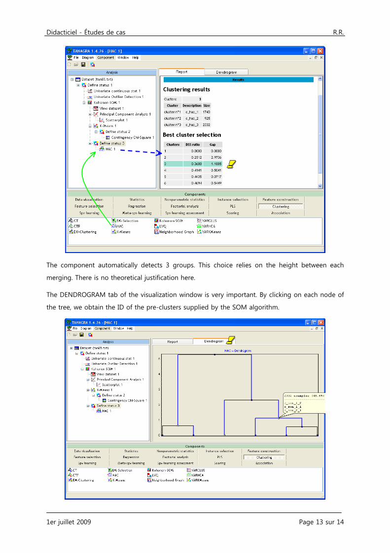
The component automatically detects 3 groups. This choice relies on the height between each

merging. There is no theoretical justification here.

The DENDROGRAM tab of the visualization window is very important. By clicking on each node of

the tree, we obtain the ID of the pre-clusters supplied by the SOM algorithm.



The white nodes of the tree states the groups computed with the HAC algorithm. If we select the

white node at right, we obtain the SOM's pre-clusters ID i.e. the individuals in this group come

from the pre-clusters (1 ; 1), (1 ; 2) et (2 ; 1).

In the table, we see the correspondence between SOM pre-clusters ID and the HAC clusters ID.

Cluster CAH Cluster SOM

1 (1 ; 3) + (2 ; 3)

2 (2 ; 2)

3 (1 ; 1) + (1 ; 2) + (2 ; 1)

The results are strikingly consistent with the theoretical consideration underlying the SOM

approach: the HAC above all merges the adjacent cells of the Kohonen’s map.

Tanagra Kohonen SOM -...

Documents

Transcript of Tanagra Kohonen SOM -...