Statistical Graphs and Calculations 18 -...

Chapter

18Statistical Graphs andCalculationsThis chapter describes how to input statistical data into lists, howto calculate the mean, maximum and other statistical values, howto perform various statistical tests, how to determine the confi-dence interval, and how to produce a distribution of statisticaldata. It also tells you how to perform regression calculations.

18-1 Before Performing Statistical Calculations

18-2 Paired-Variable Statistical Calculation Examples18-3 Calculating and Graphing Single-Variable Statistical

Data

18-4 Calculating and Graphing Paired-Variable StatisticalData

18-5 Performing Statistical Calculations

18-6 Tests18-7 Confidence Interval

18-8 Distribution

Important!• This chapter contains a number of graph screen shots. In each case, new

data values were input in order to highlight the particular characteristics ofthe graph being drawn. Note that when you try to draw a similar graph, theunit uses data values that you have input using the List function. Because ofthis, the graphs that appears on the screen when you perform a graphingoperation will probably differ somewhat from those shown in this manual.

250

18-1 Before Performing Statistical Calculations

In the Main Menu, select the STAT icon to enter the STAT Mode and display thestatistical data lists.

Use the statistical data lists to input data and to perform statistical calculations.

Use f, c, d and e to move

the highlighting around the lists.

P.251 • {GRPH} ... {graph menu}

P.270 • {CALC} ... {statistical calculation menu}

P.277 • {TEST} ... {test menu}

P.294 • {INTR} ... {confidence interval menu}

P.304 • {DIST} ... {distribution menu}

P.234 • {SRT·A}/{SRT·D} ... {ascending}/{descending} sort

P.233 • {DEL}/{DEL·A} ... deletes {highlighted data}/{all data}

P.234 • {INS} ... {inserts new cell at highlighted cell}

• The procedures you should use for data editing are identical to those you useP.229 with the list function. For details, see “17. List Function”.

251

18-2 Paired-Variable Statistical CalculationExamples

Once you input data, you can use it to produce a graph and check for tendencies.You can also use a variety of different regression calculations to analyze the data.

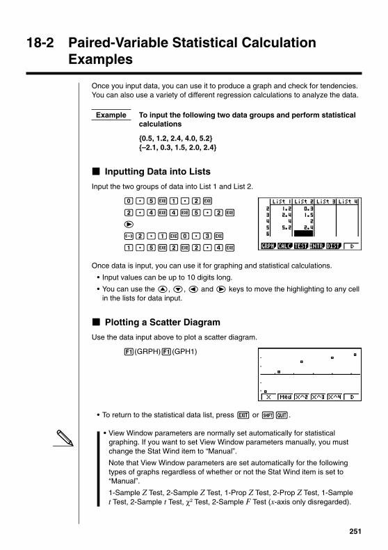
Example To input the following two data groups and perform statisticalcalculations

{0.5, 1.2, 2.4, 4.0, 5.2}{–2.1, 0.3, 1.5, 2.0, 2.4}

kkkkk Inputting Data into Lists

Input the two groups of data into List 1 and List 2.

a.fwb.cw

c.ewewf.cw

e

-c.bwa.dw

b.fwcwc.ew

Once data is input, you can use it for graphing and statistical calculations.

• Input values can be up to 10 digits long.

• You can use the f, c, d and e keys to move the highlighting to any cellin the lists for data input.

kkkkk Plotting a Scatter Diagram

Use the data input above to plot a scatter diagram.

1(GRPH)1(GPH1)

• To return to the statistical data list, press J or !Q.

• View Window parameters are normally set automatically for statisticalgraphing. If you want to set View Window parameters manually, you mustchange the Stat Wind item to “Manual”.

Note that View Window parameters are set automatically for the followingtypes of graphs regardless of whether or not the Stat Wind item is set to“Manual”.

1-Sample Z Test, 2-Sample Z Test, 1-Prop Z Test, 2-Prop Z Test, 1-Samplet Test, 2-Sample t Test, χ2 Test, 2-Sample F Test (x-axis only disregarded).

252

While the statistical data list is on the display, perform the following procedure.

!Z2(Man)

J(Returns to previous menu.)

• It is often difficult to spot the relationship between two sets of data (such asheight and shoe size) by simply looking at the numbers. Such relationshipbecome clear, however, when we plot the data on a graph, using one set ofvalues as x-data and the other set as y-data.

The default setting automatically uses List 1 data as x-axis (horizontal) values andList 2 data as y-axis (vertical) values. Each set of x/y data is a point on the scatterdiagram.

kkkkk Changing Graph Parameters

Use the following procedures to specify the graph draw/non-draw status, thegraph type, and other general settings for each of the graphs in the graph menu(GPH1, GPH2, GPH3).

While the statistical data list is on the display, press 1 (GRPH) to display thegraph menu, which contains the following items.

• {GPH1}/{GPH2}/{GPH3} ... only one graph {1}/{2}/{3} drawing

• The initial default graph type setting for all the graphs (Graph 1 through Graph3) is scatter diagram, but you can change to one of a number of other graphtypes.

P.252 • {SEL} ... {simultaneous graph (GPH1, GPH2, GPH3) selection}

P.254 • {SET} ... {graph settings (graph type, list assignments)}

• You can specify the graph draw/non-draw status, the graph type, and othergeneral settings for each of the graphs in the graph menu (GPH1, GPH2,GPH3).

• You can press any function key (1,2,3) to draw a graph regardless ofthe current location of the highlighting in the statistical data list.

1. Graph draw/non-draw status [GRPH]-[SEL]

The following procedure can be used to specify the draw (On)/non-draw (Off)status of each of the graphs in the graph menu.

uuuuuTo specify the draw/non-draw status of a graph

1. Pressing 4 (SEL) displays the graph On/Off screen.

18 - 2 Paired-Variable Statistical Calculation Examples

253

• Note that the StatGraph1 setting is for Graph 1 (GPH1 of the graph menu),StatGraph2 is for Graph 2, and StatGraph3 is for Graph 3.

2. Use the cursor keys to move the highlighting to the graph whose status youwant to change, and press the applicable function key to change the status.

• {On}/{Off} ... setting {On (draw)}/{Off (non-draw)}

• {DRAW} ... {draws all On graphs}

3. To return to the graph menu, press J.

uuuuuTo draw a graph

Example To draw a scatter diagram of Graph 3 only

1(GRPH)4(SEL) 2(Off)

cc1(On)

6(DRAW)

2. General graph settings [GRPH]-[SET]

This section describes how to use the general graph settings screen to make thefollowing settings for each graph (GPH1, GPH2, GPH3).

• Graph Type

The initial default graph type setting for all the graphs is scatter graph. You canselect one of a variety of other statistical graph types for each graph.

• List

The initial default statistical data is List 1 for single-variable data, and List 1 andList 2 for paired-variable data. You can specify which statistical data list you wantto use for x-data and y-data.

• Frequency

Normally, each data item or data pair in the statistical data list is represented on agraph as a point. When you are working with a large number of data itemshowever, this can cause problems because of the number of plot points on thegraph. When this happens, you can specify a frequency list that contains valuesindicating the number of instances (the frequency) of the data items in thecorresponding cells of the lists you are using for x-data and y-data. Once you dothis, only one point is plotted for the multiple data items, which makes the grapheasier to read.

• Mark Type

This setting lets you specify the shape of the plot points on the graph.

Paired-Variable Statistical Calculation Examples 18 - 2

254

uuuuuTo display the general graph settings screen [GRPH]-[SET]

Pressing 6 (SET) displays the general graph settings screen.

• The settings shown here are examples only. The settings on your general graphsettings screen may differ.

uuuuuStatGraph (statistical graph specification)

• {GPH1}/{GPH2}/{GPH3} ... graph {1}/{2}/{3}

uuuuuGraph Type (graph type specification)

• {Scat}/{xy}/{NPP} ... {scatter diagram}/{xy line graph}/{normal probability plot}

–––• {Hist}/{Box}/{Box}/{N·Dis}/{Brkn} ... {histogram}/{med-box graph}/{mean-box

graph}/{normal distribution curve}/{broken line graph}

• {X}/{Med}/{X^2}/{X^3}/{X^4} ... {linear regression graph}/{Med-Med graph}/{quadratic regression graph}/{cubic regression graph}/{quartic regressiongraph}

• {Log}/{Exp}/{Pwr}/{Sin}/{Lgst} ... {logarithmic regression graph}/{exponentialregression graph}/{power regression graph}/{sine regression graph}/

{logistic regression graph}

uuuuuXList (x-axis data list)

• {List1}/{List2}/{List3}/{List4}/{List5}/{List6} ... {List 1}/{List 2}/{List 3}/{List 4}/{List 5}/{List 6}

uuuuuYList (y-axis data list)

• {List1}/{List2}/{List3}/{List4}/{List5}/{List6} ... {List 1}/{List 2}/{List 3}/{List 4}/{List 5}/{List 6}

uuuuuFrequency (number of data items)

• {1} ... {1-to-1 plot}

• {List1}/{List2}/{List3}/{List4}/{List5}/{List6} ... frequency data in {List 1}/{List 2}/{List 3}/{List 4}/{List 5}/{List 6}

uuuuuMark Type (plot mark type)

• { }/{×}/{•} ... plot points: { }/{×}/{•}


255

uuuuuGraph Color (graph color specification)

• {Blue}/{Orng}/{Grn} ... {blue}/{orange}/{green}

uuuuuOutliers (outliers specification)

• {On}/{Off} ... {display}/{do not display} Med-Box outliers

kkkkk Drawing an xy Line Graph

P.254 Paired data items can be used to plot a scatter diagram. A scatter diagram where(Graph Type) the points are linked is an xy line graph.

(xy)

Press J or !Q to return to the statistical data list.

kkkkk Drawing a Normal Probability Plot

P.254 Normal probability plot contrasts the cumulative proportion of variables with the(Graph Type) cumulative proportion of a normal distribution and plots the result. The expected

(NPP) values of the normal distribution are used as the vertical axis, while the observedvalues of the variable being tested are on the horizontal axis.

Press J or !Q to return to the statistical data list.

kkkkk Selecting the Regression Type

After you graph paired-variable statistical data, you can use the function menu atthe bottom of the display to select from a variety of different types of regression.

• {X}/{Med}/{X^2}/{X^3}/{X^4}/{Log}/{Exp}/{Pwr}/{Sin}/{Lgst} ... {linear regres-sion}/{Med-Med}/{quadratic regression}/{cubic regression}/{quarticregression}/{logarithmic regression}/{exponential regression}/{powerregression}/{sine regression}/{logistic regression} calculation and graphing

• {2VAR} ... {paired-variable statistical results}

Paired-Variable Statistical Calculation Examples 18 - 2

CFX

256

kkkkk Displaying Statistical Calculation Results

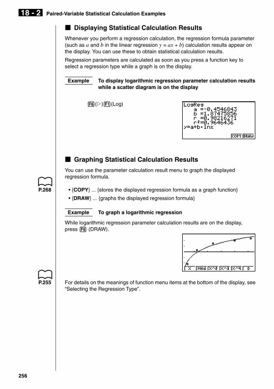
Whenever you perform a regression calculation, the regression formula parameter(such as a and b in the linear regression y = ax + b) calculation results appear onthe display. You can use these to obtain statistical calculation results.

Regression parameters are calculated as soon as you press a function key toselect a regression type while a graph is on the display.

Example To display logarithmic regression parameter calculation resultswhile a scatter diagram is on the display

6(g)1(Log)

kkkkk Graphing Statistical Calculation Results

You can use the parameter calculation result menu to graph the displayedregression formula.

P.268 • {COPY} ... {stores the displayed regression formula as a graph function}

• {DRAW} ... {graphs the displayed regression formula}

Example To graph a logarithmic regression

While logarithmic regression parameter calculation results are on the display,press 6 (DRAW).

P.255 For details on the meanings of function menu items at the bottom of the display, see“Selecting the Regression Type”.


257

Calculating and Graphing Single-Variable Statistical Data 18 - 3

18-3 Calculating and Graphing Single-VariableStatistical Data

Single-variable data is data with only a single variable. If you are calculating theaverage height of the members of a class for example, there is only one variable(height).

Single-variable statistics include distribution and sum. The following types ofgraphs are available for single-variable statistics.

kkkkk Drawing a Histogram (Bar Graph)

From the statistical data list, press 1 (GRPH) to display the graph menu, press6 (SET), and then change the graph type of the graph you want to use (GPH1,GPH2, GPH3) to histogram (bar graph).

Data should already be input in the statistical data list (see “Inputting Data intoLists”). Draw the graph using the procedure described under “Changing GraphParameters”.

⇒6(DRAW)

The display screen appears as shown above before the graph is drawn. At thispoint, you can change the Start and pitch values.

kkkkk Med-box Graph (Med-Box)

This type of graph lets you see how a large number of data items are groupedwithin specific ranges. A box encloses all the data in an area from the first quartile(Q1) to the third quartile (Q3), with a line drawn at the median (Med). Lines (calledwhiskers) extend from either end of the box up to the minimum and maximum ofthe data.

From the statistical data list, press 1 (GRPH) to display the graph menu, press6 (SET), and then change the graph type of the graph you want to use (GPH1,GPH2, GPH3) to med-box graph.

P.251P.252

P.254(Graph Type)

(Hist)

6

P.254(Graph Type)

(Box)

Q1 Med Q3 maxX

minX

258

To plot the data that falls outside the box, first specify “MedBox” as the graphtype. Then, on the same screen you use to specify the graph type, turn the outliersitem “On”, and draw the graph.

kkkkk Mean-box Graph

This type of graph shows the distribution around the mean when there is a largenumber of data items. A line is drawn at the point where the mean is located, andthen a box is drawn so that it extends below the mean up to the populationstandard deviation (o – xσn) and above the mean up to the population standarddeviation (o + xσn). Lines (called whiskers) extend from either end of the box up tothe minimum (minX) and maximum (maxX) of the data.

From the statistical data list, press 1 (GRPH) to display the graph menu, press6 (SET), and then change the graph type of the graph you want to use (GPH1,GPH2, GPH3) to mean-box graph.

kkkkk Normal Distribution Curve

P.254 The normal distribution curve is graphed using the following normal distribution(Graph Type) function.

(N·Dis)y =

1

(2 π) xσn

e–

2xσn2

(x–x) 2

The distribution of characteristics of items manufactured according to some fixedstandard (such as component length) fall within normal distribution. The more dataitems there are, the closer the distribution is to normal distribution.

From the statistical data list, press 1 (GRPH) to display the graph menu, press6 (SET), and then change the graph type of the graph you want to use (GPH1,GPH2, GPH3) to normal distribution.

18 - 3 Calculating and Graphing Single-Variable Statistical Data

P.254(Graph Type)

(Box)

Note :

This function is not usually used inthe classrooms in U.S. Please useMed-box Graph, instead.

o – xσn o o + xσn

minX

maxX

259

Calculating and Graphing Single-Variable Statistical Data 18 - 3

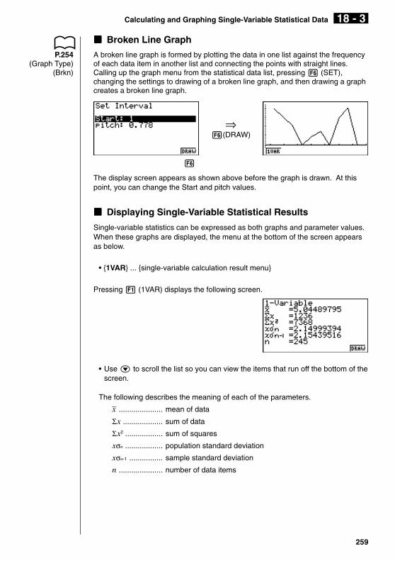
kkkkk Broken Line Graph

P.254 A broken line graph is formed by plotting the data in one list against the frequency(Graph Type) of each data item in another list and connecting the points with straight lines.

(Brkn) Calling up the graph menu from the statistical data list, pressing 6 (SET),changing the settings to drawing of a broken line graph, and then drawing a graphcreates a broken line graph.

⇒6(DRAW)

6

The display screen appears as shown above before the graph is drawn. At thispoint, you can change the Start and pitch values.

kkkkk Displaying Single-Variable Statistical Results

Single-variable statistics can be expressed as both graphs and parameter values.When these graphs are displayed, the menu at the bottom of the screen appearsas below.

• {1VAR} ... {single-variable calculation result menu}

Pressing 1 (1VAR) displays the following screen.

• Use c to scroll the list so you can view the items that run off the bottom of thescreen.

The following describes the meaning of each of the parameters._x ..................... mean of data

Σx ................... sum of data

Σx2 .................. sum of squares

xσn .................. population standard deviation

xσn-1 ................ sample standard deviation

n ..................... number of data items

260

minX ............... minimum

Q1 .................. first quartile

Med ................ median

Q3 .................. third quartile_x –xσn ............ data mean – population standard deviation_x + xσn ............ data mean + population standard deviation

maxX .............. maximum

Mod ................ mode

• Press 6 (DRAW) to return to the original single-variable statistical graph.

18 - 3 Calculating and Graphing Single-Variable Statistical Data

261

18-4 Calculating and Graphing Paired-VariableStatistical Data

Under “Plotting a Scatter Diagram,” we displayed a scatter diagram and thenperformed a logarithmic regression calculation. Let’s use the same procedure tolook at the various regression functions.

kkkkk Linear Regression Graph

P.254 Linear regression plots a straight line that passes close to as many data points aspossible, and returns values for the slope and y-intercept (y-coordinate when x =0) of the line.

The graphic representation of this relationship is a linear regression graph.

(Graph Type) !Q1(GRPH)6(SET)c

(Scatter) 1(Scat)

(GPH1) !Q1(GRPH)1(GPH1)

(X) 1(X)

1 2 3 4 5 6

6(DRAW)

a ...... regression coefficient (slope)

b ...... regression constant term (y-intercept)

r ....... correlation coefficient

r2 ...... coefficient of determination

kkkkk Med-Med Graph

P.254 When it is suspected that there are a number of extreme values, a Med-Medgraph can be used in place of the least squares method. This is also a type oflinear regression, but it minimizes the effects of extreme values. It is especiallyuseful in producing highly reliable linear regression from data that includesirregular fluctuations, such as seasonal surveys.

2(Med)

1 2 3 4 5 6

262

6(DRAW)

a ...... Med-Med graph slope

b ...... Med-Med graph y-intercept

kkkkk Quadratic/Cubic/Quartic Regression Graph

P.254 A quadratic/cubic/quartic regression graph represents connection of the datapoints of a scatter diagram. It actually is a scattering of so many points that areclose enough together to be connected. The formula that represents this isquadratic/cubic/quartic regression.

Ex. Quadratic regression

3(X^ 2)

1 2 3 4 5 6

6(DRAW)

Quadratic regression

a ...... regression second coefficient

b ...... regression first coefficient

c ...... regression constant term (y-intercept)

Cubic regression

a ...... regression third coefficient

b ...... regression second coefficient

c ...... regression first coefficient

d ...... regression constant term (y-intercept)

Quartic regression

a ...... regression fourth coefficient

b ...... regression third coefficient

c ...... regression second coefficient

d ...... regression first coefficient

e ...... regression constant term (y-intercept)

18 - 4 Calculating and Graphing Paired-Variable Statistical Data

263

Calculating and Graphing Paired-Variable Statistical Data 18 - 4

kkkkk Logarithmic Regression Graph

P.254 Logarithmic regression expresses y as a logarithmic function of x. The standardlogarithmic regression formula is y = a + b × Inx, so if we say that X = Inx, theformula corresponds to linear regression formula y = a + bX.

6(g)1(Log)

1 2 3 4 5 6

6(DRAW)

a ...... regression constant term

b ...... regression coefficient

r ...... correlation coefficient

r2 ..... coefficient of determination

kkkkk Exponential Regression Graph

P.254 Exponential regression expresses y as a proportion of the exponential function ofx. The standard exponential regression formula is y = a × ebx, so if we take thelogarithms of both sides we get Iny = Ina + bx. Next, if we say Y = Iny, and A = Ina,the formula corresponds to linear regression formula Y = A + bx.

6(g)2(Exp)

1 2 3 4 5 6

6(DRAW)

a ...... regression coefficient

b ...... regression constant term



264


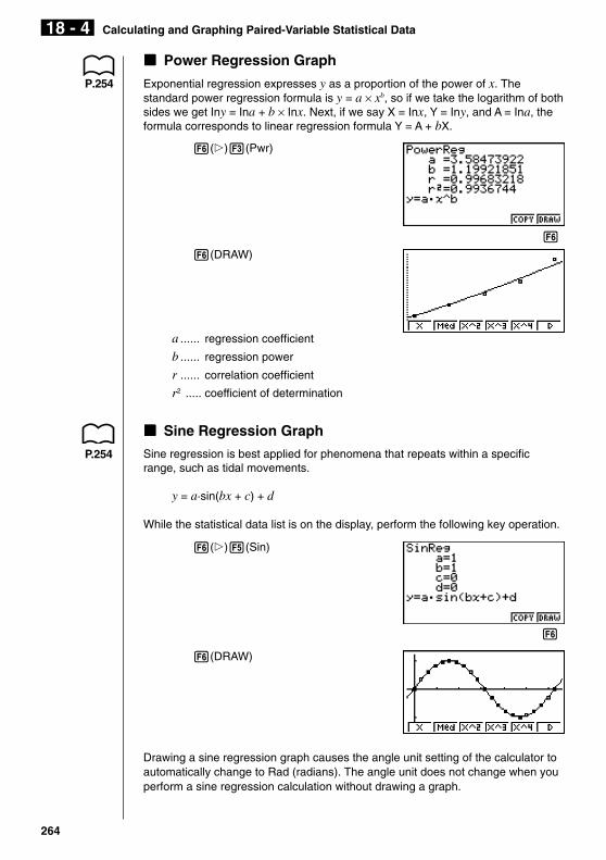
kkkkk Power Regression Graph

P.254 Exponential regression expresses y as a proportion of the power of x. Thestandard power regression formula is y = a × xb, so if we take the logarithm of bothsides we get Iny = Ina + b × Inx. Next, if we say X = Inx, Y = Iny, and A = Ina, theformula corresponds to linear regression formula Y = A + bX.

6(g)3(Pwr)

1 2 3 4 5 6

6(DRAW)

a ...... regression coefficient

b ...... regression power



kkkkk Sine Regression Graph

Sine regression is best applied for phenomena that repeats within a specificrange, such as tidal movements.

y = a·sin(bx + c) + d

While the statistical data list is on the display, perform the following key operation.

6(g)5(Sin)

6(DRAW)

Drawing a sine regression graph causes the angle unit setting of the calculator toautomatically change to Rad (radians). The angle unit does not change when youperform a sine regression calculation without drawing a graph.

P.254

6

265


Gas bills, for example, tend to be higher during the winter when heater use ismore frequent. Periodic data, such as gas usage, is suitable for application of sineregression.

Example To perform sine regression using the gas usage data shownbelow

List 1 (Month Data){1, 2, 3, 4, 5, 6, 7, 8, 9, 10, 11, 12, 13, 14, 15, 16, 17, 18, 19, 20, 21,22, 23, 24, 25, 26, 27, 28, 29, 30, 31, 32, 33, 34, 35, 36, 37, 38, 39,40, 41, 42, 43, 44, 45, 46, 47, 48}

List 2 (Gas Usage Meter Reading){130, 171, 159, 144, 66, 46, 40, 32, 32, 39, 44, 112, 116, 152, 157,109, 130, 59, 40, 42, 33, 32, 40, 71, 138, 203, 162, 154, 136, 39,32, 35, 32, 31, 35, 80, 134, 184, 219, 87, 38, 36, 33, 40, 30, 36, 55,94}

Input the above data and plot a scatter diagram.

1(GRPH)1(GPH1)

Execute the calculation and produce sine regression analysis results.

6(g)5(Sin)

Display a sine regression graph based on the analysis results.

6(DRAW)

kkkkk Logistic Regression Graph

Logistic regression is best applied for phenomena in which there is a continualincrease in one factor as another factor increases until a saturation point isreached. Possible applications would be the relationship between medicinaldosage and effectiveness, advertising budget and sales, etc.

6

P.254

266

y = C1 + ae–bx

6(g)6(g)1(Lgst)

6(DRAW)

Example Imagine a country that started out with a television diffusionrate of 0.3% in 1966, which grew rapidly until diffusion reachedvirtual saturation in 1980. Use the paired statistical data shownbelow, which tracks the annual change in the diffusion rate, toperform logistic regression.

List1(Year Data)

{66, 67, 68, 69, 70, 71, 72, 73, 74, 75, 76, 77, 78, 79, 80, 81, 82, 83}

List2(Diffusion Rate)

{0.3, 1.6, 5.4, 13.9, 26.3, 42.3, 61.1, 75.8, 85.9, 90.3, 93.7, 95.4, 97.8, 97.8,98.2, 98.5, 98.9, 98.8}

1(GRPH)1(GPH1)

Perform the calculation, and the logistic regression analysis values appear on thedisplay.

6(g)6(g)1(Lgst)


6

6

267

Draw a logistic regression graph based on the parameters obtained from theanalytical results.

6(DRAW)

kkkkk Residual Calculation

Actual plot points (y-coordinates) and regression model distance can be calcu-lated during regression calculations.

P.6 While the statistical data list is on the display, recall the set up screen to specify alist (“List 1” through “List 6”) for “Resid List”. Calculated residual data is stored inthe specified list.

The vertical distance from the plots to the regression model will be stored.

Plots that are higher than the regression model are positive, while those that arelower are negative.

Residual calculation can be performed and saved for all regression models.

Any data already existing in the selected list is cleared. The residual of each plot isstored in the same precedence as the data used as the model.

kkkkk Displaying Paired-Variable Statistical Results

Paired-variable statistics can be expressed as both graphs and parameter values.When these graphs are displayed, the menu at the bottom of the screen appearsas below.

• {2VAR} ... {paired-variable calculation result menu}

Pressing 4 (2VAR) displays the following screen.


268

• Use c to scroll the list so you can view the items that run off the bottom of thescreen.

_x ..................... mean of xList data

Σx ................... sum of xList data

Σx2 .................. sum of squares of xList data

xσn .................. population standard deviation of xList data

xσn-1 ................ sample standard deviation of xList data

n ..................... number of xList data items_y ..................... mean of yList data

Σy ................... sum of yList data

Σy2 .................. sum of squares of yList data

yσn .................. population standard deviation of yList data

yσn-1 ................ sample standard deviation of yList data

Σxy ..................sum of the product of data stored in xList and yList

minX ............... minimum of xList data

maxX .............. maximum of xList data

minY ............... minimum of yList data

maxY .............. maximum of yList data

kkkkk Copying a Regression Graph Formula to the Graph Mode

After you perform a regression calculation, you can copy its formula to theGRAPH Mode.

The following are the functions that are available in the function menu at thebottom of the display while regression calculation results are on the screen.

• {COPY} ... {stores the displayed regression formula to the GRAPH Mode}

• {DRAW} ... {graphs the displayed regression formula}

1. Press 5 (COPY) to copy the regression formula that produced the displayeddata to the GRAPH Mode.

Note that you cannot edit regression formulas for graph formulas in the GRAPHMode.

2. Press w to save the copied graph formula and return to the previousregression calculation result display.


269

kkkkk Multiple Graphs

You can draw more than one graph on the same display by using the procedureP.252 under “Changing Graph Parameters” to set the graph draw (On)/non-draw (Off)

status of two or all three of the graphs to draw “On”, and then pressing 6(DRAW). After drawing the graphs, you can select which graph formula to usewhen performing single-variable statistic or regression calculations.

6(DRAW)

P.254 1(X)

• The text at the top of the screen indicates the currently selected graph(StatGraph1 = Graph 1, StatGraph2 = Graph 2, StatGraph3 = Graph 3).

1. Use f and c to change the currently selected graph. The graph name atthe top of the screen changes when you do.

c

2. When graph you want to use is selected, press w.

P.259 Now you can use the procedures under “Displaying Single-Variable StatisticalP.267 Results” and “Displaying Paired-Variable Statistical Results” to perform statistical

calculations.


270

18 - 5 Performing Statistical Calculations

18-5 Performing Statistical Calculations

All of the statistical calculations up to this point were performed after displaying agraph. The following procedures can be used to perform statistical calculationsalone.

uuuuuTo specify statistical calculation data lists

You have to input the statistical data for the calculation you want to perform andspecify where it is located before you start a calculation. Display the statisticaldata and then press 2(CALC)6 (SET).

The following is the meaning for each item.

1Var XList ....... specifies list where single-variable statistic x values (XList)are located

1Var Freq ........ specifies list where single-variable frequency values(Frequency) are located

2Var XList ....... specifies list where paired-variable statistic x values (XList)are located

2Var YList ....... specifies list where paired-variable statistic y values (YList)are located

2Var Freq ........ specifies list where paired-variable frequency values(Frequency) are located

• Calculations in this section are performed based on the above specifications.

kkkkk Single-Variable Statistical Calculations

In the previous examples from “Drawing a Normal Probability Plot” and “Histogram(Bar Graph)” to “Line Graph,” statistical calculation results were displayed after thegraph was drawn. These were numeric expressions of the characteristics ofvariables used in the graphic display.

These values can also be directly obtained by displaying the statistical data listand pressing 2 (CALC) 1 (1VAR).

271

Performing Statistical Calculations 18 - 5

Now you can use the cursor keys to view the characteristics of the variables.

For details on the meanings of these statistical values, see “Displaying Single-Variable Statistical Results”.

kkkkk Paired-Variable Statistical Calculations

In the previous examples from “Linear Regression Graph” to “Logistic RegressionGraph,” statistical calculation results were displayed after the graph was drawn.These were numeric expressions of the characteristics of variables used in thegraphic display.

These values can also be directly obtained by displaying the statistical data listand pressing 2 (CALC) 2 (2VAR).

Now you can use the cursor keys to view the characteristics of the variables.

P.267 For details on the meanings of these statistical values, see “Displaying Paired-Variable Statistical Results”.

kkkkk Regression Calculation

In the explanations from “Linear Regression Graph” to “Logistic RegressionGraph,” regression calculation results were displayed after the graph was drawn.Here, the regression line and regression curve is represented by mathematicalexpressions.

You can directly determine the same expression from the data input screen.

Pressing 2 (CALC) 3 (REG) displays a function menu, which contains thefollowing items.

• {X}/{Med}/{X^2}/{X^3}/{X^4}/{Log}/{Exp}/{Pwr}/{Sin}/{Lgst} ... {linear regres-sion}/{Med-Med}/{quadratic regression}/{cubic regression}/{quarticregression}/{logarithmic regression}/{exponential regression}/{powerregression}/{sine regression}{logistic regression} parameters

Example To display single-variable regression parameters

2(CALC)3(REG)1(X)

The meaning of the parameters that appear on this screen is the same as that for“Linear Regression Graph” to “Logistic Regression Graph”.

P.259

272

kkkkk Estimated Value Calculation ( , )

After drawing a regression graph with the STAT Mode, you can use the RUNMode to calculate estimated values for the regression graph's x and y parameters.

• Note that you cannot obtain estimated values for a Med-Med, quadraticregression, cubic regression, quartic regression, sine regression, or logisticregression graph.

Example To perform power regression using thenearby data and estimate the values of

and when xi = 40 and yi = 1000

1. In the Main Menu, select the STAT icon and enter the STAT Mode.

2. Input data into the list and draw the power regression graph*.

3. In the Main Menu, select the RUN icon and enter the RUN Mode.

4. Press the keys as follows.

ea(value of xi)

K5(STAT)2( )w

The estimated value is displayed for xi = 40.

baaa(value of yi)

1( )w

The estimated value is displayed for yi = 1000.

1(GRPH)6(SET)c

1(Scat)c

1(List1)c

2(List2)c

1(1)c

1( )J

!Z1(Auto)J1(GRPH)1(GPH1)6(g)

3(Pwr)6(DRAW)


*(Graph Type)

(Scatter)

(XList)

(YList)

(Frequency)

(Mark Type)

(Auto)

(Pwr)

xi yi28 2410

30 303333 3895

35 4491

38 5717

273

kkkkk Normal Probability Distribution Calculation and Graphing

You can calculate and graph normal probability distributions for single-variablestatistics.

uuuuuNormal probability distribution calculations

Use the RUN Mode to perform normal probability distribution calculations. PressK in the RUN Mode to display the option number and then press 6 (g)3 (PROB) 6 (g) to display a function menu, which contains the followingitems.

• {P(}/{Q(}/{R(} ... obtains normal probability {P(t)}/{Q(t)}/{R(t)} value

• {t(} ... {obtains normalized variate t(x) value}

• Normal probability P(t), Q(t), and R(t), and normalized variate t(x) arecalculated using the following formulas.

P(t) Q(t) R(t)

duu2

duu2

duu2

Example The following table shows the results of measurements of theheight of 20 college students. Determine what percentage ofthe students fall in the range 160.5 cm to 175.5 cm. Also, inwhat percentile does the 175.5 cm tall student fall?

Class no. Height (cm) Frequency

1 158.5 1

2 160.5 1

3 163.3 2

4 167.5 2

5 170.2 3

6 173.3 4

7 175.5 2

8 178.6 2

9 180.4 2

10 186.7 1

1. In the STAT Mode, input the height data into List 1 and the frequency data intoList 2.


274

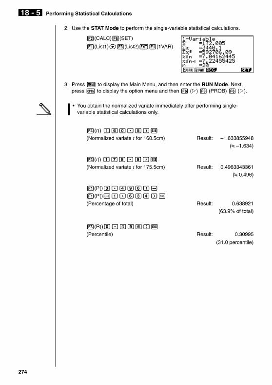
2. Use the STAT Mode to perform the single-variable statistical calculations.

2(CALC)6(SET)

1(List1)c3(List2)J1(1VAR)

3. Press m to display the Main Menu, and then enter the RUN Mode. Next,press K to display the option menu and then 6 (g) 3 (PROB) 6 (g).

• You obtain the normalized variate immediately after performing single-variable statistical calculations only.

4(t() bga.f)w

(Normalized variate t for 160.5cm) Result: –1.633855948

( –1.634)

4(t() bhf.f)w

(Normalized variate t for 175.5cm) Result: 0.4963343361

( 0.496)

1(P()a.ejg)-

1(P()-b.gde)w

(Percentage of total) Result: 0.638921

(63.9% of total)

3(R()a.ejg)w

(Percentile) Result: 0.30995

(31.0 percentile)


275

kkkkk Normal Probability Graphing

You can graph a normal probability distribution with Graph Y = in the Sketch Mode.

Example To graph normal probability P(0.5)

Perform the following operation in the RUN Mode.

!4(Sketch)1(Cls)w

5(GRPH)1(Y=)K6(g)3(PROB)

6(g)1(P()a.f)w

The following shows the View Window settings for the graph.

Ymin ~ Ymax–0.1 0.45

Xmin ~ Xmax–3.2 3.2


276

18-6 Tests

The Z Test provides a variety of different standardization-based tests. They makeit possible to test whether or not a sample accurately represents the populationwhen the standard deviation of a population (such as the entire population of acountry) is known from previous tests. Z testing is used for market research andpublic opinion research, that need to be performed repeatedly.

1-Sample Z Test tests for unknown population mean when the populationstandard deviation is known.

2-Sample Z Test tests the equality of the means of two populations based onindependent samples when both population standard deviations are known.

1-Prop Z Test tests for an unknown proportion of successes.

2-Prop Z Test tests to compare the proportion of successes from two populations.

The t Test uses the sample size and obtained data to test the hypothesis that thesample is taken from a particular population. The hypothesis that is the opposite ofthe hypothesis being proven is called the null hypothesis, while the hypothesisbeing proved is called the alternative hypothesis. The t-test is normally applied totest the null hypothesis. Then a determination is made whether the null hypothesisor alternative hypothesis will be adopted.

When the sample shows a trend, the probability of the trend (and to what extent itapplies to the population) is tested based on the sample size and variance size.Inversely, expressions related to the t test are also used to calculate the samplesize required to improve probability. The t test can be used even when thepopulation standard deviation is not known, so it is useful in cases where there isonly a single survey.

1-Sample t Test tests the hypothesis for a single unknown population mean whenthe population standard deviation is unknown.

2-Sample t Test compares the population means when the population standarddeviations are unknown.

LinearReg t Test calculates the strength of the linear association of paired data.

In addition to the above, a number of other functions are provided to check therelationship between samples and populations.

χ2 Test tests hypotheses concerning the proportion of samples included in each ofa number of independent groups. Mainly, it generates cross-tabulation of twocategorical variables (such as yes, no) and evaluates the independence of thesevariables. It could be used, for example, to evaluate the relationship betweenwhether or not a driver has ever been involved in a traffic accident and thatperson’s knowledge of traffic regulations.

277

2-Sample F Test tests the hypothesis that there will be no change in the result fora population when a result of a sample is composed of multiple factors and one ormore of the factors is removed. It could be used, for example, to test the carcino-genic effects of multiple suspected factors such as tobacco use, alcohol, vitamindeficiency, high coffee intake, inactivity, poor living habits, etc.

ANOVA tests the hypothesis that the population means of the samples are equalwhen there are multiple samples. It could be used, for example, to test whether ornot different combinations of materials have an effect on the quality and life of afinal product.

The following pages explain various statistical calculation methods based on theprinciples described above. Details concerning statistical principles andterminology can be found in any standard statistics textbook.

While the statistical data list is on the display, press 3 (TEST) to display the testmenu, which contains the following items.

• {Z}/{t}/{CHI}/{F} ... {Z}/{t}/{χ2}/{F} test

• {ANOV} ... {analysis of variance (ANOVA)}

About data type specificationFor some types of tests you can select data type using the following menu.

• {List}/{Var} ... specifies {list data}/{parameter data}

kkkkk Z Test

You can use the following menu to select from different types of Z Test.

• {1-S}/{2-S}/{1-P}/{2-P} ... {1-Sample}/{2-Sample}/{1-Prop}/{2-Prop} Z Test

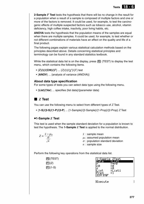
uuuuu1-Sample Z Test

This test is used when the sample standard deviation for a population is known totest the hypothesis. The 1-Sample Z Test is applied to the normal distribution.

Z = o – 0

σµ

n

o : sample meanµo : assumed population meanσ : population standard deviationn : sample size

Perform the following key operations from the statistical data list.

3(TEST)

1(Z)

1(1-S)

Tests 18 - 6

278

The following shows the meaning of each item in the case of list data specifica-tion.

Data ................ data type

µ ..................... population mean value test conditions (“G µ0” specifiestwo-tail test, “< µ0” specifies lower one-tail test, “> µ0”specifies upper one-tail test.)

µ0 .................... assumed population mean

σ ..................... population standard deviation (σ > 0)

List .................. list whose contents you want to use as data (List 1 to 6)

Freq ................ frequency (1 or List 1 to 6)

Execute .......... executes a calculation or draws a graph

The following shows the meaning of parameter data specification items that aredifferent from list data specification.

o ..................... sample mean

n ..................... sample size (positive integer)

Example To perform a 1-Sample Z Test for one list of data

For this example, we will perform a µ < µ0 test for the data List1= {11.2, 10.9, 12.5, 11.3, 11.7}, when µ0 = 11.5 and σ = 3.

1(List)c2(<)c

bb.fw

dw

1(List1)c1(1)c

1(CALC)

µ<11.5 ............ assumed population mean and direction of test

z ...................... z value

p ..................... p-value

o ..................... sample mean


n ..................... sample size

6(DRAW) can be used in place of 1(CALC) in the final Execute line to draw agraph.

18 - 6 Tests

279

Perform the following key operations from the statistical result screen.

J(To data input screen)

cccccc(To Execute line)

6(DRAW)

uuuuu2-Sample Z Test

This test is used when the sample standard deviations for two populations areknown to test the hypothesis. The 2-Sample Z Test is applied to the normaldistribution.

Z = o1 – o2

σn1

12 σ

n2

22

+

o1 : sample 1 meano2 : sample 2 meanσ1 : population standard deviation of sample 1σ2 : population standard deviation of sample 2n1 : sample 1 sizen2 : sample 2 size


3(TEST)

1(Z)

2(2-S)

The following shows the meaning of each item in the case of list data specification.

Data ................ data type

µ1 .................... population mean value test conditions (“G µ2” specifies two-tail test, “< µ2” specifies one-tail test where sample 1 issmaller than sample 2, “> µ2” specifies one-tail test wheresample 1 is greater than sample 2.)

σ1 .................... population standard deviation of sample 1 (σ1 > 0)


List1 ................ list whose contents you want to use as sample 1 data


Freq1 .............. frequency of sample 1



Tests 18 - 6

280


o1 .................... sample 1 mean

n1 .................... sample 1 size (positive integer)

o2 .................... sample 2 mean


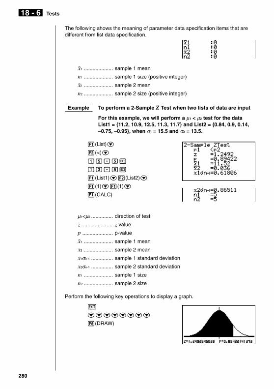
Example To perform a 2-Sample Z Test when two lists of data are input

For this example, we will perform a µ1 < µ2 test for the dataList1 = {11.2, 10.9, 12.5, 11.3, 11.7} and List2 = {0.84, 0.9, 0.14,–0.75, –0.95}, when σ1 = 15.5 and σ2 = 13.5.

1(List)c

2(<)c

bf.fw

bd.fw

1(List1)c2(List2)c

1(1)c1(1)c

1(CALC)

µ1<µ2 ............... direction of test

z ...................... z value

p ..................... p-value

o1 .................... sample 1 mean

o2 .................... sample 2 mean

x1σn-1 ............... sample 1 standard deviation


n1 .................... sample 1 size

n2 .................... sample 2 size

Perform the following key operations to display a graph.

J

cccccccc

6(DRAW)

18 - 6 Tests

281

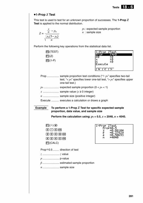
uuuuu1-Prop Z Test

This test is used to test for an unknown proportion of successes. The 1-Prop ZTest is applied to the normal distribution.

Z = nx

np0(1– p0)

– p0

p0 : expected sample proportionn : sample size


3(TEST)

1(Z)

3(1-P)

Prop ................ sample proportion test conditions (“G p0” specifies two-tailtest, “< p0” specifies lower one-tail test, “> p0” specifies upperone-tail test.)

p0 .................... expected sample proportion (0 < p0 < 1)

x ..................... sample value (x > 0 integer)



Example To perform a 1-Prop Z Test for specific expected sampleproportion, data value, and sample size

Perform the calculation using: p0 = 0.5, x = 2048, n = 4040.

1(G)c

a.fw

caeiw

eaeaw

1(CALC)

PropG0.5 ........ direction of test

z ...................... z value

p ...................... p-value

p̂ ...................... estimated sample proportion

n ...................... sample size

Tests 18 - 6

282

The following key operations can be used to draw a graph.

J

cccc

6(DRAW)

uuuuu2-Prop Z Test

This test is used to compare the proportion of successes. The 2-Prop Z Test isapplied to the normal distribution.

Z = n1

x1

n2

x2–

p(1 – p )n1

1n2

1+

x1 : sample 1 data valuex2 : sample 2 data valuen1 : sample 1 sizen2 : sample 2 sizep̂ : estimated sample proportion


3(TEST)

1(Z)

4(2-P)

p1 .................... sample proportion test conditions (“G p2” specifies two-tailtest, “< p2” specifies one-tail test where sample 1 is smallerthan sample 2, “> p2” specifies one-tail test where sample 1is greater than sample 2.)

x1 .................... sample 1 data value (x1 > 0 integer)


x2 .................... sample 2 data value (x2 > 0 integer)



Example To perform a p1 > p2 2-Prop Z Test for expected sampleproportions, data values, and sample sizes

Perform a p1 > p2 test using: x1 = 225, n1 = 300, x2 = 230, n2 = 300.

18 - 6 Tests

283

3(>)c

ccfw

daaw

cdaw

daaw

1(CALC)

p1>p2 ............... direction of test

z ...................... z value

p ..................... p-value

p̂ 1 .................... estimated proportion of population 1

p̂ 2 .................... estimated proportion of population 2

p̂ ..................... estimated sample proportion

n1 .................... sample 1 size

n2 .................... sample 2 size


J

ccccc

6(DRAW)

kkkkk t Test

You can use the following menu to select a t test type.

• {1-S}/{2-S}/{REG} ... {1-Sample}/{2-Sample}/{LinearReg} t Test

uuuuu1-Sample t Test

This test uses the hypothesis test for a single unknown population mean when thepopulation standard deviation is unknown. The 1-Sample t Test is applied to t-distribution.

t =o – 0µ

σx n–1

n

o : sample meanµ0 : assumed population meanxσn-1 : sample standard deviationn : sample size


3(TEST)

2(t)

1(1-S)

Tests 18 - 6

284


Data ................ data type

µ ..................... population mean value test conditions (“G µ0” specifies two-tail test, “< µ0” specifies lower one-tail test, “> µ0” specifiesupper one-tail test.)

µ0 .................... assumed population mean

List .................. list whose contents you want to use as data

Freq ................ frequency



o ..................... sample mean

xσn-1 ................ sample standard deviation (xσn-1 > 0)


Example To perform a 1-Sample t Test for one list of data

For this example, we will perform a µ GGGGG µ0 test for the dataList1 = {11.2, 10.9, 12.5, 11.3, 11.7}, when µ0 = 11.3.

1(List)c

1(G)c

bb.dw

1(List1)c1(1)c

1(CALC)

µ G 11.3 .......... assumed population mean and direction of test

t ...................... t value

p ..................... p-value

o ..................... sample mean


n ..................... sample size


J

ccccc

6(DRAW)

18 - 6 Tests

285

uuuuu2-Sample t Test

2-Sample t Test compares the population means when the population standarddeviations are unknown. The 2-Sample t Test is applied to t-distribution.

The following applies when pooling is in effect.

t = o1 – o2

n1

1 + n2

1xp n–12σ

xp n–1 = σ n1 + n2 – 2(n1–1)x1 n–12 +(n2–1)x2 n–12σ σ

df = n1 + n2 – 2

The following applies when pooling is not in effect.

t = o1 – o2

x1 n–12σ

n1+

x2 n–12σ

n2

df = 1C 2

n1–1+

(1–C )2

n2–1

C = x1 n–1

2σn1

+x2 n–1

2σn2

x1 n–12σ

n1


3(TEST)

2(t)

2(2-S)

Tests 18 - 6

o1 : sample 1 meano2 : sample 2 mean

x1σn-1 : sample 1 standarddeviation


n1 : sample 1 sizen2 : sample 2 size

xpσn-1 : pooled sample standarddeviation

df : degrees of freedom

o1 : sample 1 meano2 : sample 2 mean



n1 : sample 1 sizen2 : sample 2 sizedf : degrees of freedom

286


Data ................ data type

µ1 .................... sample mean value test conditions (“G µ2” specifies two-tailtest, “< µ2” specifies one-tail test where sample 1 is smallerthan sample 2, “> µ2” specifies one-tail test where sample 1 isgreater than sample 2.)





Pooled ............ pooling On or Off



o1 .................... sample 1 mean

x1σn-1 ............... sample 1 standard deviation (x1σn-1 > 0)


o2 .................... sample 2 mean



Example To perform a 2-Sample t Test when two lists of data are input

For this example, we will perform a µ1 GGGGG µ2 test for the dataList1 = {55, 54, 51, 55, 53, 53, 54, 53} and List2 = {55.5, 52.3,51.8, 57.2, 56.5} when pooling is not in effect.

1(List)c1(G)c

1(List1)c2(List2)c

1(1)c1(1)

c2(Off)c

1(CALC)

18 - 6 Tests

287

µ1Gµ2 .............. direction of test

t ...................... t value

p ..................... p-value

df .................... degrees of freedom

o1 .................... sample 1 mean

o2 .................... sample 2 mean



n1 .................... sample 1 size

n2 .................... sample 2 size


J

ccccccc

6(DRAW)

The following item is also shown when Pooled = On.

xpσn-1 ............... pooled sample standard deviation

uuuuuLinearReg t Test

LinearReg t Test treats paired-variable data sets as (x, y) pairs, and uses themethod of least squares to determine the most appropriate a, b coefficients of thedata for the regression formula y = a + bx. It also determines the correlationcoefficient and t value, and calculates the extent of the relationship between x andy.

b = Σ( x – o)( y – p)i=1

n

Σ(x – o)2

i=1

na = p – bo t = r n – 2

1 – r2

a : interceptb : slope of the line


3(TEST)

2(t)

3(REG)

Tests 18 - 6

288


β & ρ ............... p-value test conditions (“G 0” specifies two-tail test, “< 0”specifies lower one-tail test, “> 0” specifies upper one-tailtest.)

XList ............... list for x-axis data

YList ............... list for y-axis data

Freq ................ frequency

Execute .......... executes a calculation

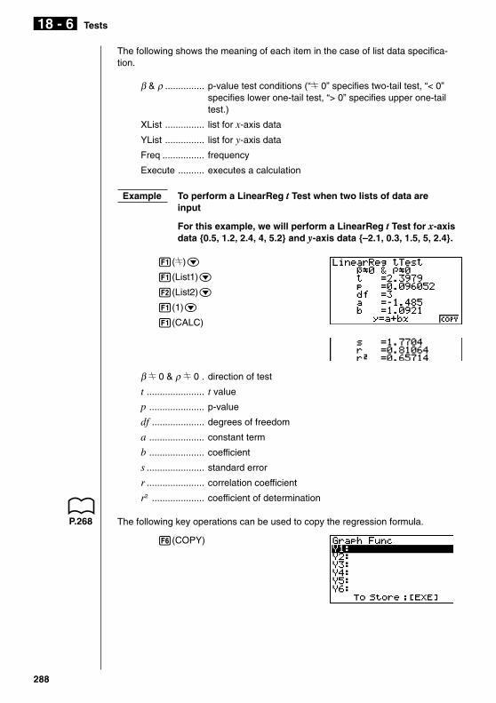
Example To perform a LinearReg t Test when two lists of data areinput

For this example, we will perform a LinearReg t Test for x-axisdata {0.5, 1.2, 2.4, 4, 5.2} and y-axis data {–2.1, 0.3, 1.5, 5, 2.4}.

1(G)c

1(List1)c

2(List2)c

1(1)c

1(CALC)

β G 0 & ρ G 0 . direction of test

t ...................... t value

p ..................... p-value


a ..................... constant term

b ..................... coefficient

s ...................... standard error

r ...................... correlation coefficient

r2 .................... coefficient of determination

The following key operations can be used to copy the regression formula.

6(COPY)

P.268

18 - 6 Tests

289

kkkkk Other Tests

uuuuuχ2 Test

χ2 Test sets up a number of independent groups and tests hypotheses related tothe proportion of the sample included in each group. The χ2 Test is applied todichotomous variables (variable with two possible values, such as yes/no).

expected counts

Fij = Σxiji=1

k

×Σxijj=1

k

ΣΣi=1 j=1

xij

χ2 = ΣΣ Fiji=1

k (xij – Fij)2

j=1

For the above, data must already be input in a matrix using the MAT Mode.


3(TEST)

3(CHI)

Next, specify the matrix that contains the data. The following shows the meaningof the above item.

Observed ........ name of matrix (A to Z) that contains observed counts (all cellspositive integers)


The matrix must be at least two lines by two columns. An error occurs if thematrix has only one line or one column.

Example To perform a χ2 Test on a specific matrix cell

For this example, we will perform a χ2 Test for Mat A, whichcontains the following data.

Mat A = 1 4

5 10

1(Mat A)c

1(CALC)

Tests 18 - 6

290

χ2 .................... χ2 value

p ..................... p-value


Expected ........ expected counts (Result is always stored in MatAns.)

The following key operations can be used to display the graph.

J

c

6(DRAW)

uuuuu2-Sample F Test

2-Sample F Test tests the hypothesis that when a sample result is composed ofmultiple factors, the population result will be unchanged when one or some of thefactors are removed. The F Test is applied to the F distribution.

F = x1 n–1

2σx2 n–1

2σ


3(TEST)

4(F)

The following is the meaning of each item in the case of list data specification.

Data ................ data type

σ1 .................... population standard deviation test conditions (“G σ2”specifies two-tail test, “< σ2” specifies one-tail test wheresample 1 is smaller than sample 2, “> σ2” specifies one-tailtest where sample 1 is greater than sample 2.)






18 - 6 Tests

291






Example To perform a 2-Sample F Test when two lists of data are input

For this example, we will perform a 2-Sample F Test for thedata List1 = {0.5, 1.2, 2.4, 4, 5.2} and List2 = {–2.1, 0.3, 1.5, 5,2.4}.

1(List)c1(G)c

1(List1)c2(List2)c

1(1)c1(1)c

1(CALC)

σ1Gσ2 .............. direction of test

F ..................... F value

p ..................... p-value



o1 .................... sample 1 mean

o2 .................... sample 2 mean

n1 .................... sample 1 size

n2 .................... sample 2 size


J

cccccc

6(DRAW)

Tests 18 - 6

292

uuuuuAnalysis of Variance (ANOVA)

ANOVA tests the hypothesis that when there are multiple samples, the means ofthe populations of the samples are all equal.

MSMSe

F =

SSFdf

MS =

SSeEdf

MSe =

SS = Σni (oi – o)2

i=1

k

SSe = Σ(ni – 1)xi σn–12

i=1

k

Fdf = k – 1

Edf = Σ(ni – 1)i=1

k


3(TEST)

5(ANOV)

The following is the meaning of each item in the case of list data specification.

How Many ...... number of samples




A value from 2 through 6 can be specified in the How Many line, so up to sixsamples can be used.

Example To perform one-way ANOVA (analysis of variance) whenthree lists of data are input

For this example, we will perform analysis of variance for thedata List1 = {6, 7, 8, 6, 7}, List2 = {0, 3, 4, 3, 5, 4, 7} andList3 = {4, 5, 4, 6, 6, 7}.

k : number of populationsoi : mean of each listxiσn-1 : standard deviation of each listni : size of each listo : mean of all listsF : F valueMS : factor mean squaresMSe : error mean squaresSS : factor sum of squaresSSe : error sum of squaresFdf : factor degrees of freedomEdf : error degrees of freedom

18 - 6 Tests

293

2(3)c

1(List1)c

2(List2)c

3(List3)c

1(CALC)

F ..................... F value

p ..................... p-value


Fdf .................. factor degrees of freedom

SS ................... factor sum of squares

MS .................. factor mean squares

Edf .................. error degrees of freedom

SSe ................. error sum of squares

MSe ................ error mean squares

Tests 18 - 6

294

18 - 8 Confidence Interval

18-7 Confidence Interval

A confidence interval is a range (interval) that includes a statistical value, usuallythe population mean.

A confidence interval that is too broad makes it difficult to get an idea of where thepopulation value (true value) is located. A narrow confidence interval, on the otherhand, limits the population value and makes it difficult to obtain reliable results.The most commonly used confidence levels are 95% and 99%. Raising theconfidence level broadens the confidence interval, while lowering the confidencelevel narrows the confidence level, but it also increases the chance of accidentlyoverlooking the population value. With a 95% confidence interval, for example, thepopulation value is not included within the resulting intervals 5% of the time.

When you plan to conduct a survey and then t test and Z test the data, you mustalso consider the sample size, confidence interval width, and confidence level.The confidence level changes in accordance with the application.

1-Sample Z Interval calculates the confidence interval when the populationstandard deviation is known.

2-Sample Z Interval calculates the confidence interval when the populationstandard deviations of two samples are known.

1-Prop Z Interval calculates the confidence interval when the proportion is notknown.

2-Prop Z Interval calculates the confidence interval when the proportions of twosamples are not known.

1-Sample t Interval calculates the confidence interval for an unknown populationmean when the population standard deviation is unknown.

2-Sample t Interval calculates the confidence interval for the difference betweentwo population means when both population standard deviations are unknown.

While the statistical data list is on the display, press 4 (INTR) to display theconfidence interval menu, which contains the following items.

• {Z}/{t} ... {Z}/{t} confidence interval calculation

About data type specificationFor some types of confidence interval calculation you can select data type using thefollowing menu.

• {List}/{Var} ... specifies {List data}/{parameter data}

295

kkkkk Z Confidence Interval

You can use the following menu to select from the different types of Z confidenceinterval.

• {1-S}/{2-S}/{1-P}/{2-P} ... {1-Sample}/{2-Sample}/{1-Prop}/{2-Prop} Z Interval

uuuuu1-Sample Z Interval

1-Sample Z Interval calculates the confidence interval for an unknown populationmean when the population standard deviation is known.

The following is the confidence interval.

However, α is the level of significance. The value 100 (1 – α) % is the confidencelevel.

When the confidence level is 95%, for example, inputting 0.95 produces 1 – 0.95 =0.05 = α.


4(INTR)

1(Z)

1(1-S)


Data ................ data type

C-Level ........... confidence level (0 < C-Level < 1)

σ ..................... population standard deviation (σ > 0)

List .................. list whose contents you want to use as sample data

Freq ................ sample frequency



o ..................... sample mean


Left = o – Z α2

σn

Right = o + Z α2

σn

Confidence Interval 18 - 7

296

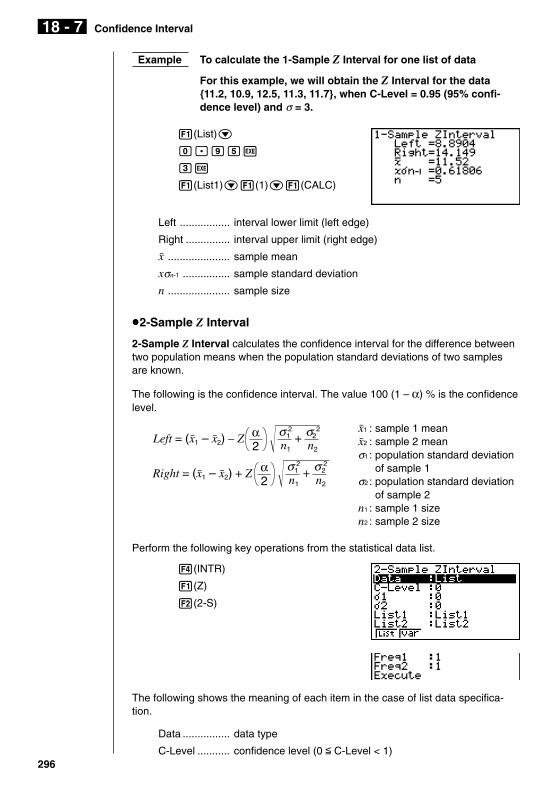
Example To calculate the 1-Sample Z Interval for one list of data

For this example, we will obtain the Z Interval for the data{11.2, 10.9, 12.5, 11.3, 11.7}, when C-Level = 0.95 (95% confi-dence level) and σ = 3.

1(List)c

a.jfw

dw

1(List1)c1(1)c1(CALC)

Left ................. interval lower limit (left edge)

Right ............... interval upper limit (right edge)

o ..................... sample mean


n ..................... sample size

uuuuu2-Sample Z Interval

2-Sample Z Interval calculates the confidence interval for the difference betweentwo population means when the population standard deviations of two samplesare known.

The following is the confidence interval. The value 100 (1 – α) % is the confidencelevel.

Left = (o1 – o2) – Z α2

Right = (o1 – o2) + Z α2

n1

12σ +

n2

22σ

n1

12σ +

n2

22σ

o1 : sample 1 meano2 : sample 2 meanσ1 : population standard deviation

of sample 1σ2 : population standard deviation

of sample 2n1 : sample 1 sizen2 : sample 2 size


4(INTR)

1(Z)

2(2-S)


Data ................ data type



297









o1 .................... sample 1 mean


o2 .................... sample 2 mean


Example To calculate the 2-Sample Z Interval when two lists of data areinput

For this example, we will obtain the 2-Sample Z Interval for thedata 1 = {55, 54, 51, 55, 53, 53, 54, 53} and data 2 = {55.5, 52.3,51.8, 57.2, 56.5} when C-Level = 0.95 (95% confidence level),σ1 = 15.5, and σ2 = 13.5.

1(List)c

a.jfw

bf.fw

bd.fw

1(List1)c2(List2)c1(1)c

1(1)c1(CALC)



o1 .................... sample 1 mean

o2 .................... sample 2 mean



n1 .................... sample 1 size

n2 .................... sample 2 size


298

uuuuu1-Prop Z Interval

1-Prop Z Interval uses the number of data to calculate the confidence interval foran unknown proportion of successes.


Left = – Z α2

Right = + Z

xn n

1nx

nx1–

xn

α2 n

1nx

nx1–

n : sample sizex : data


4(INTR)

1(Z)

3(1-P)

Data is specified using parameter specification. The following shows the meaningof each item.


x ..................... data (0 or positive integer)



Example To calculate the 1-Prop Z Interval using parameter valuespecification

For this example, we will obtain the 1-Prop Z Interval whenC-Level = 0.99, x = 55, and n = 100.

a.jjw

ffw

baaw

1(CALC)



p̂ ..................... estimated sample proportion

n ..................... sample size


299

uuuuu2-Prop Z Interval

2-Prop Z Interval uses the number of data items to calculate the confidenceinterval for the defference between the proportion of successes in two populations.


Left = – – Z α2

x1n1

x2n2 n1

n1

x1 1– n1

x1

+ n2

n2

x2 1– n2

x2

Right = – + Z α2

x1n1

x2n2 n1

n1

x1 1– n1

x1

+ n2

n2

x2 1– n2

x2

n1, n2 : sample sizex1, x2 : data


4(INTR)

1(Z)

4(2-P)



x1 .................... sample 1 data value (x1 > 0)


x2 .................... sample 2 data value (x2 > 0)


Execute .......... Executes a calculation

Example To calculate the 2-Prop Z Interval using parameter valuespecification

For this example, we will obtain the 2-Prop Z Interval whenC-Level = 0.95, x1 = 49, n1 = 61, x2 = 38 and n2 = 62.

a.jfw

ejwgbw

diwgcw

1(CALC)




300

p̂ 1 .................... estimated sample propotion for sample 1

p̂ 2 .................... estimated sample propotion for sample 2

n1 .................... sample 1 size

n2 .................... sample 2 size

kkkkk t Confidence Interval

You can use the following menu to select from two types of t confidence interval.

• {1-S}/{2-S} ... {1-Sample}/{2-Sample} t Interval

uuuuu1-Sample t Interval

1-Sample t Interval calculates the confidence interval for an unknown populationmean when the population standard deviation is unknown.


Left = o– tn – 1α2

Right = o+ tn – 1α2

x n–1σn

x n–1σn


4(INTR)

2(t)

1(1-S)


Data ................ data type



Freq ................ sample frequency

Execute .......... execute a calculation


o ..................... sample mean

xσn-1 ................ sample standard deviation (xσn-1 > 0)



301

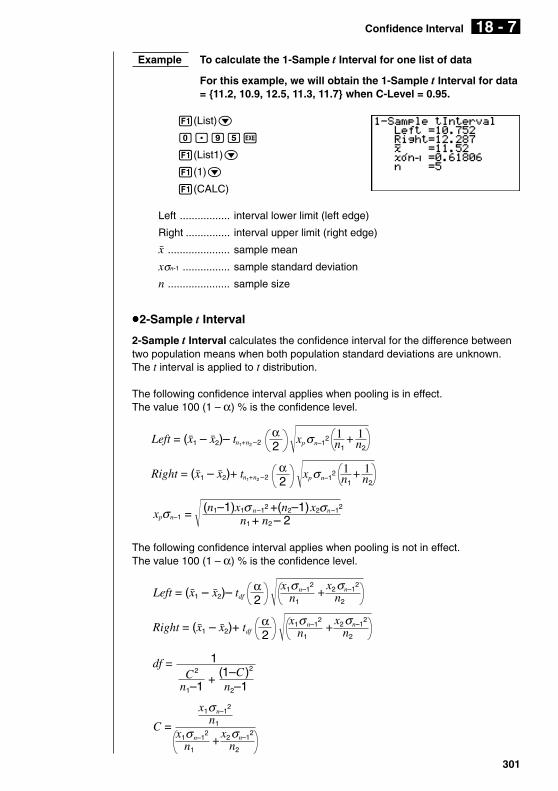
Example To calculate the 1-Sample t Interval for one list of data

For this example, we will obtain the 1-Sample t Interval for data= {11.2, 10.9, 12.5, 11.3, 11.7} when C-Level = 0.95.

1(List)c

a.jfw

1(List1)c

1(1)c

1(CALC)



o ..................... sample mean


n ..................... sample size

uuuuu2-Sample t Interval

2-Sample t Interval calculates the confidence interval for the difference betweentwo population means when both population standard deviations are unknown.The t interval is applied to t distribution.

The following confidence interval applies when pooling is in effect.The value 100 (1 – α) % is the confidence level.

Left = (o1 – o2)– t α2

Right = (o1 – o2)+ t α2

n1+n2 –2 n1

1 + n2

1xp n–12σ

n1+n2 –2 n1

1 + n2

1xp n–12σ

The following confidence interval applies when pooling is not in effect.The value 100 (1 – α) % is the confidence level.

Left = (o1 – o2)– tdfα2

Right = (o1 – o2)+ tdfα2

+n1

x1 n–12σ

n2

x2 n–12σ

+n1

x1 n–12σ

n2

x2 n–12σ

C =

df = 1C

2

n1–1+

(1–C )2

n2–1

+n1

x1 n–12σn1

x1 n–12σ

n2

x2 n–12σ


xp n–1 = σ n1 + n2 – 2(n1–1)x1 n–12 +(n2–1)x2 n–12σ σ

302


4(INTR)

2(t)

2(2-S)


Data ................ data type






Pooled ............ pooling On or Off



o1 .................... sample 1 mean



o2 .................... sample 2 mean




303

Example To calculate the 2-Sample t Interval when two lists of data areinput

For this example, we will obtain the 2-Sample t Interval for data 1= {55, 54, 51, 55, 53, 53, 54, 53} and data 2 = {55.5, 52.3, 51.8, 57.2,56.5} without pooling when C-Level = 0.95.

1(List)c

a.jfw

1(List1)c2(List2)c1(1)c

1(1)c2(Off)c1(CALC)




o1 .................... sample 1 mean

o2 .................... sample 2 mean



n1 .................... sample 1 size

n2 .................... sample 2 size

The following item is also shown when Pooled = On.



304

18-8 Distribution

There is a variety of different types of distribution, but the most well-known is“normal distribution,” which is essential for performing statistical calculations.Normal distribution is a symmetrical distribution centered on the greatest occur-rences of mean data (highest frequency), with the frequency decreasing as youmove away from the center. Poisson distribution, geometric distribution, andvarious other distribution shapes are also used, depending on the data type.

Certain trends can be determined once the distribution shape is determined. Youcan calculate the probability of data taken from a distribution being less than aspecific value.

For example, distribution can be used to calculate the yield rate when manufactur-ing some product. Once a value is established as the criteria, you can calculatenormal probability density when estimating what percent of the products meet thecriteria. Conversely, a success rate target (80% for example) is set up as thehypothesis, and normal distribution is used to estimate the proportion of theproducts will reach this value.

Normal probability density calculates the probability density of normal distribu-tion from a specified x value.

Normal distribution probability calculates the probability of normal distributiondata falling between two specific values.

Inverse cumulative normal distribution calculates a value that represents thelocation within a normal distribution for a specific cumulative probability.

Student- t probability density calculates t probability density from a specified xvalue.

Student- t distribution probability calculates the probability of t distribution datafalling between two specific values.

Like t distribution, distribution probability can also be calculated for chi-square, F,binomial, Poisson, and geometric distributions.

While the statistical data list is on the display, press 5 (DIST) to display thedistribution menu, which contains the following items.

• {NORM}/{t}/{CHI}/{F}/{BINM}/{POISN}/{GEO} ... {normal}/{t}/{χ2}/{F}/{binomial}/{Poisson}/{geometric} distribution

About data type specificationFor some types of distribution you can select data type using the following menu.

• {List}/{Var} ... specifies {list data}/{parameter data}

305

kkkkk Normal Distribution

You can use the following menu to select from the different types of calculation.

• {Npd}/{Ncd}/{InvN} ... {normal probability density}/{normal distributionprobability}/{inverse cumulative normal distribution} calculation

uuuuuNormal probability density

Normal probability density calculates the probability density of normal distributionfrom a specified x value. Normal probability density is applied to the standardnormal distribution.

πσ2f(x) = 1 e

–2 2σ

(x – µ)2µ(σ > 0)


5(DIST)

1(NORM)

1(Npd)


x ..................... data

σ ..................... standard deviation (σ > 0)

µ ..................... mean


• Specifying σ = 1 and µ = 0 specifies standard normal distribution.

Example To calculate the normal probability density for a specificparameter value

For this example, we will calculate the normal probabilitydensity when x = 36, σ = 2 and µ = 35.

dgw

cw

dfw

1(CALC)

p(x) ................. normal probability density

Distribution 18 - 8

306


J

ccc

6(DRAW)

uuuuuNormal distribution probability

Normal distribution probability calculates the probability of normal distribution datafalling between two specific values.

πσ2p = 1 e

–dx 2 2σ

(x – µ)2µ

a

b∫a : lower boundaryb : upper boundary


5(DIST)

1(NORM)

2(Ncd)


Lower ............. lower boundary

Upper ............. upper boundary


µ ..................... mean


Example To calculate the normal distribution probability for a specificparameter value

For this example, we will calculate the normal distributionprobability when lower boundary = – ∞ (–1E99), upperboundary = 36, σ = 2 and µ = 35.

-bEjjw

dgw

cw

dfw

1(CALC)

prob ................ normal distribution probability

18 - 8 Distribution

307

• This calculator performs the above calculation using the following:

∞ = 1E99, –∞ = –1E99

uuuuuInverse cumulative normal distribution

Inverse cumulative normal distribution calculates a value that represents thelocation within a normal distribution for a specific cumulative probability.

Specify the probability and use this formula to obtain the integration interval.


5(DIST)

1(NORM)

3(InvN)


Area ................ probability value (0 < Area < 1)


µ ..................... mean


Example To calculate inverse cumulative normal distribution for aspecific parameter value

For this example, we will determine inverse cumulative normaldistribution when probability value = 0.691462, σ = 2 and µ = 35.

a.gjbegcw

cw

dfw

1(CALC)

x ..................... inverse cumulative normal distribution (upper boundary ofintegration interval)

Distribution 18 - 8

Upper boundary ofintegration intervalα = ?

f (x)dx = p−∞∫

308

kkkkk Student-t Distribution

You can use the following menu to select from the different types of Student-tdistribution.

• {tpd}/{tcd} ... {Student-t probability density}/{Student-t distribution probability}calculation

uuuuuStudent-t probability density

Student-t probability density calculates t probability density from a specified xvalue.

f (x) = Γ

Γ

dfπ

– df+12

2df2

df + 1df

1 + x2


5(DIST)

2(t)

1(tpd)


x ..................... data

df .................... degrees of freedom (df >0)


Example To calculate Student-t probability density for a specificparameter value

For this example, we will calculate Student-t probability densitywhen x = 1 and degrees of freedom = 2.

bw

cw

1(CALC)

p(x) ................. Student-t probability density

18 - 8 Distribution

309

Perform the following key operation to display a graph.

J

cc

6(DRAW)

uuuuuStudent-t distribution probability

Student-t distribution probability calculates the probability of t distribution datafalling between two specific values.

p = Γ

Γ

dfπ2df

2df + 1

– df+12

df1 + x2

dxa

b

∫a : lower boundaryb : upper boundary


5(DIST)

2(t)

2(tcd)




df .................... degrees of freedom (df > 0)


Example To calculate Student-t distribution probability for a specificparameter value

For this example, we will calculate Student-t distributionprobability when lower boundary = –2, upper boundary = 3, anddegrees of freedom = 18.

-cw

dw

biw

1(CALC)

prob ................ Student-t distribution probability

Distribution 18 - 8

310

kkkkk Chi-square Distribution

You can use the following menu to select from the different types of chi-squaredistribution.

• {Cpd}/{Ccd} ... {χ2 probability density}/{χ2 distribution probability} calculation

uuuuuχ2 probability density

χ2 probability density calculates the probability density function for the χ2

distribution at a specified x value.

f(x) =

Γ

1

2df

df2 x e

21

df2

–1x2

– (x > 0)


5(DIST)

3(CHI)

1(Cpd)


x ..................... data

df .................... degrees of freedom (positive integer)


Example To calculate χ2 probability density for a specific parametervalue

For this example, we will calculate χ2 probability density whenx = 1 and degrees of freedom = 3.

bw

dw

1(CALC)

p(x) ................. χ2 probability density

18 - 8 Distribution

311


J

cc

6(DRAW)

uuuuuχ2 distribution probability

χ2 distribution probability calculates the probability of χ2 distribution data fallingbetween two specific values.

p =

Γ

1

2df

df2

x e dx21 df

2–1

x2

–

a

b



5(DIST)

3(CHI)

2(Ccd)




df .................... degrees of freedom (positive integer)


Example To calculate χ2 distribution probability for a specific parametervalue

For this example, we will calculate χ2 distribution probabilitywhen lower boundary = 0, upper boundary = 19.023, anddegrees of freedom = 9.

aw

bj.acdw

jw

1(CALC)

prob ................ χ2 distribution probability

Distribution 18 - 8

312

kkkkk F Distribution

You can use the following menu to select from the different types of F distribution.

• {Fpd}/{Fcd} ... {F probability density}/{F distribution probability} calculation

uuuuuF probability density

F probability density calculates the probability density function for the Fdistribution at a specified x value.

Γ

n2x

dn

n2

–1

2n

Γ2

n + d

Γ 2d d

nx1 +

n + d2

f (x) = –

(x > 0)


5(DIST)

4(F)

1(Fpd)


x ..................... data

n-df ................. numerator degrees of freedom (positive integer)

d-df ................. denominator degrees of freedom (positive integer)


Example To calculate F probability density for a specific parametervalue

For this example, we will calculate F probability density whenx = 1, n-df = 24, and d-df = 19.

bw

cew

bjw

1(CALC)

p(x) ................. F probability density


J

ccc

6(DRAW)

18 - 8 Distribution

313

uuuuuF distribution probability

F distribution probability calculates the probability of F distribution data fallingbetween two specific values.

p = Γ

n2

dxxdn

n2

–1

2n

Γ2

n + d

Γ 2d d

nx1 +

n + d2

–

a

b



5(DIST)

4(F)

2(Fcd)




n-df ................. numerator degrees of freedom (positive integer)

d-df ................. denominator degrees of freedom (positive integer)


Example To calculate F distribution probability for a specific parametervalue

For this example, we will calculate F distribution probabilitywhen lower boundary = 0, upper boundary = 1.9824, n-df = 19and d-df = 16.

aw

b.jicew

bjw

bgw

1(CALC)

prob ................ F distribution probability

kkkkk Binomial Distribution

You can use the following menu to select from the different types of binomialdistribution.

• {Bpd}/{Bcd} ... {binomial probability}/{binomial cumulative density}calculation

Distribution 18 - 8

314

uuuuuBinomial probability

Binomial probability calculates a probability at specified value for the discretebinomial distribution with the specified number of trials and probability of successon each trial.

f (x) = nCxpx(1–p)n – x (x = 0, 1, ·······, n) p : success probability(0 < p < 1)

n : number of trials


5(DIST)

5(BINM)

1(Bpd)

The following shows the meaning of each item when data is specified using listspecification.

Data ................ data type


Numtrial .......... number of trials (positive integer)

p ..................... success probability (0 < p < 1)


The following shows the meaning of a parameter data specification item that isdifferent from list data specification.

x ..................... integer from 0 to n

Example To calculate binomial probability for one list of data

For this example, we will calculate binomial probability fordata = {10, 11, 12, 13, 14} when Numtrial = 15 and successprobability = 0.6.

1(List)c

1(List1)c

bfw

a.gw

1(CALC)

probability when x = 10





18 - 8 Distribution

315

uuuuuBinomial cumulative density

Binomial cumulative density calculates a cumulative probability at specified valuefor the discrete binomial distribution with the specified number of trials andprobability of success on each trial.


5(DIST)

5(BINM)

2(Bcd)


Data ................ data type


Numtrial .......... number of trials (positive integer)




x ..................... integer from 0 to n

Example To calculate binomial cumulative probability for one list of data

For this example, we will calculate binomial cumulativeprobability for data = {10, 11, 12, 13, 14} when Numtrial = 15and success probability = 0.6.

1(List)c

1(List1)c

bfw

a.gw

1(CALC)

cumulative probability when x = 10





Distribution 18 - 8

316

kkkkk Poisson Distribution

You can use the following menu to select from the different types of Poissondistribution.

• {Ppd}/{Pcd} ... {Poisson probability}/{Poisson cumulative density} calculation

uuuuuPoisson probability

Poisson probability calculates a probability at specified value for the discrete Poissondistribution with the specified mean.

f(x) = x!

e– xµµ(x = 0, 1, 2, ···) µ : mean (µ > 0)


5(DIST)

6(g)

1(POISN)

1(Ppd)


Data ................ data type


µ ..................... mean (µ > 0)



x ..................... value

Example To calculate Poisson probability for one list of data

For this example, we will calculate Poisson probability for data= {2, 3, 4} when µ = 6.

1(List)c

1(List1)c

gw

1(CALC)




18 - 8 Distribution

317

uuuuuPoisson cumulative density

Poisson cumulative density calculates a cumulative probability at specified valuefor the discrete Poisson distribution with the specified mean.


5(DIST)

6(g)

1(POISN)

2(Pcd)


Data ................ data type


µ ..................... mean (µ > 0)



x ..................... value

Example To calculate Poisson cumulative probability for one list of data

For this example, we will calculate Poisson cumulativeprobability for data = {2, 3, 4} when µ = 6.

1(List)c

1(List1)c

gw

1(CALC)




kkkkk Geometric Distribution

You can use the following menu to select from the different types of geometricdistribution.

• {Gpd}/{Gcd} ... {geometric probability}/{geometric cumulative density}calculation

Distribution 18 - 8

318

uuuuuGeometric probability

Geometric probability calculates a probability at specified value, the number of thetrial on which the first success occurs, for the discrete geometric distribution withthe specified probability of success.

f (x) = p(1– p) x – 1 (x = 1, 2, 3, ···)


5(DIST)

6(g)

2(GEO)

1(Gpd)


Data ................ data type





x ..................... value

• Positive integer number is calculated whether list data (Data:List) or x value(Data:variable) is specified.

Example To calculate geometric probability for one list of data

For this example, we will calculate geometric probability for data= {3, 4, 5} when p = 0.4.

1(List)c

1(List1)c

a.ew

1(CALC)




18 - 8 Distribution

319

uuuuuGeometric cumulative density

Geometric cumulative density calculates a cumulative probability at specifiedvalue, the number of the trial on which the first success occurs, for the discretegeometric distribution with the specified probability of success.


5(DIST)

6(g)

2(GEO)

2(Gcd)


Data ................ data type





x ..................... value

• Positive integer number is calculated whether list data (Data:List) or x value(Data:variable) is specified.

Example To calculate geometric cumulative probability for one list ofdata

For this example, we will calculate geometric cumulativeprobability for data = {2, 3, 4} when p = 0.5.

1(List)c

1(List1)c

a.fw

1(CALC)




Distribution 18 - 8

Statistical Graphs and Calculations 18 -...

Documents

Transcript of Statistical Graphs and Calculations 18 -...