Statistical Inference on Random Graphs:

Comparative Power Analyses via Monte Carlo

Henry Pao1, Glen A. Coppersmith2, and Carey E. Priebe1

Johns Hopkins University

1Department of Applied Mathematics and Statistics

2Human Language Technology Center of Excellence

July 4, 2010

(JCGS final revision)

Abstract

We present a comparative power analysis, via Monte Carlo, of various graph invariants used as

statistics for testing graph homogeneity versus a “chatter” alternative – the existence of a local region of

excessive activity. Our results indicate that statistical inference on random graphs, even in a relatively

simple setting, can be decidedly non-trivial. We find that none of the graph invariants considered is

uniformly most powerful throughout our space of alternatives.

1

1 Introduction

Graphs are useful for representing a wide range of natural phenomenon. Thus, detecting anomalies within

graphs may provide information relevant to making inferences for a variety of applications, such as corporate

email traffic analysis (Priebe et al. 2005), examinations of turn-taking behavior (Grothendieck et al. 2008),

entity extraction from text (Doddington et al. 2004), peer to peer application analysis (Sen et al. 2004),

or analysis of social networks (Leenders 1995). Specifically, we are interested in being able to infer when a

graph has a local region of excessive connectivity. In order to detect such changes we consider seven graph

invariants: size, maximum degree, maximum average degree, scan statistic, number of triangles, clustering

coefficient, and average path length. We design an inferential setting in which we evaluate the statistical

power of these various graph invariants for detecting anomalies.

Our inference task is to differentiate homogeneous graphs from heterogenous graphs. Specifically, our

null hypothesis (H0) is that all vertices have the same probability of connection. The alternative hypothesis

(HA) is that there exists a subset of vertices that are (probabilistically) more highly inter-connected than the

rest of the graph. In both cases, we consider the simple scenario in which all edges are mutually independent.

For example, if the vertices represent the senders and recipients of email (actors) and each edge represents

an email between two actors, then H0 states that each actor communicates with each other actor with equal

probability while HA states that there is a subset of actors which share excessive email communication

amongst each other – there is increased “chatter” among these vertices. See, for instance, Newman (2003)

and Newman et al. (2006) for a general discussion of related applications.

Our results indicate that no invariant among those considered herein is universally most powerful for

detecting increased local chatter.

1.1 Random Graphs

To model these phenomena and the effectiveness of the graph invariants for detecting anomalous behavior,

we use undirected graphs G ∈ Gn, the collection of all graphs on the n vertices V = 1, ..., n. We denote

the vertex set V = V (G) and edge set E = E(G); thus G = (V,E). To denote edges in E, we use the

notation euv for u, v ∈ V (it is said that vertices u and v are adjacent). We will not consider weighted or

parallel edges. We will not consider loops, so if euv ∈ E then u 6= v. Our graphs are undirected, so there is

no distinction between euv and evu.

1.2 Null Hypothesis

Our null hypothesis (H0) is that the observed graph is drawn from an Erdos-Renyi (ER) random graph

model (Bollobas 2001); that is, each of the(n2

)possible edges exists independently with a given probability

1

p

p

q

n−m vertices

m vertices

1

Figure 1: HA: The “kidney and egg” graph, κ(n, p,m, q). The small “egg” represents the m vertices (VA)that exhibit chatter (each edge occurring with probability q). The “kidney” is the population of n − mvertices which are not exhibiting chatter (each edge occurring with probability p < q). Edges between avertex in the kidney and a vertex in the egg occur with probability p.

p ∈ [0, 1). Again, V = 1, ..., n, so H0: ER(n, p).

1.3 Alternative Hypothesis

Our alternative hypothesis (HA) – local chatter – is the κ random graph model, κ(n, p,m, q). Again,

V = 1, ..., n. A subset of m vertices (VA ⊂ V , |VA| = m, m ∈ 2, . . . , n ) are connected with probability

q where q > p. The remaining n −m vertices are connected with probability p, just like the entire graph

under H0, to represent the portion of the population not “chattering”. Edges between a vertex in VA and a

vertex in V \VA occur with probability p. Again, all edges are independent of one another. We parameterize

our alternative by θ ∈ ΘA = 2, . . . , n × (p, 1]. This κ graph is referred to as the “kidney and egg” graph

as depicted in Figure 1. So, HA: κ(n, p,m, q) with (m, q) ∈ ΘA.

Our comparative power investigation consists of quantifying the ability of various graph invariants to

distinguish a homogeneous ER(n, p) graph from our local “chatter” alternative κ(n, p,m, q).

2

1.4 Graph Preliminaries

Graph theory preliminaries are available in many textbooks; see, for instance, West (2001). We present here

the basics required for our analysis.

1.4.1 Size and Order

The size of a graph G, denoted size (G) = |E(G)|, is the number of edges. Likewise, the order of a graph G,

denoted order (G) = |V (G)|, is the number of vertices.

1.4.2 Distance

The distance between any two vertices is measured by the minimum number of edges required to traverse

between them. For vertices u and v, this is denoted by l(u, v). If euv ∈ E(G) then l(u, v) = 1; l(u, u) = 0

for all u; and if no path exists between u and v then l(u, v) =∞.

1.4.3 Degree

The degree of vertex v, denoted d(v), is the number of edges incident to v. Since we allow only a single edge

between two vertices and no loops, d(v) is also the number of vertices connected to v.

1.4.4 Adjacency Matrix

The adjacency matrix A = A(G) is an n×n symmetric, hollow (zeros on the diagonal), binary matrix where

n = order (G). If auv denotes the (u, v)th element of A, then auv = 1 if and only if euv ∈ E(G).

1.4.5 Induced Subgraphs

Given a collection of vertices V ′ ⊂ V , the induced subgraph Ω(V ′;G) is defined to be the graph (V ′, E′)

where euv ∈ E′ if and only if u ∈ V ′, v ∈ V ′ and euv ∈ E. In essence, Ω(V ′;G) is the collection of V ′ vertices

and the edges from G connecting any pair of those vertices.

1.4.6 Neighborhoods

To study local activity of a graph, we use neighborhoods to provide a notion of locality. The kth order

neighborhood of v ∈ V is defined as Nk[v;G] = u ∈ V (G) : l(v, u) ≤ k.

2 Graph Invariants

We examine the power of seven graph invariants, acting as test statistics, to detect excessive local activity.

The statistics we examine are: size, maximum degree, maximum average degree (both via a greedy approxi-

3

mation and via an eigenvalue approximation), scan statistic, number of triangles, clustering coefficient, and

average path length. In all cases, a large value of the invariant is evidence in favor of HA.

2.1 Definitions

2.1.1 Size

The size of a graph is the number of edges in the graph, given by

size (G) = |E(G)|. (1)

This simplest graph invariant is a global measure of activity; as such, it would not be expected to have good

power characteristics against κ(n, p,m, q) for small values of m.

2.1.2 Maximum Degree

The maximum degree δ(G) is given by

δ(G) = maxv∈V

d(v) (2)

and is the simplest local graph invariant.

2.1.3 Maximum Average Degree

The maximum average degree over all subgraphs of G is denoted MAD(G). If d(v) is the degree of vertex v,

then the average degree of a graph G is given by

d(G) =1|V |

∑v∈V

d(v) =2 size(G)order(G)

. (3)

Thus the maximum average degree invariant is given by

MAD(G) = maxΩ⊂G

d(Ω) (4)

where the maximum is over all induced subgraphs of G. (Notice that it suffices to consider only induced

subgraphs, since any subgraph with fewer edges than its related induced subgraph will have a lower average

degree.)

Since this invariant is difficult to compute exactly, we resort to consideration of two approximations to

the maximum average degree, MADg(G) and MADe(G), such that

MADg(G) ≤ MAD(G) ≤ MADe(G). (5)

4

Greedy MAD

We consider a primitive greedy algorithm MADg(G) to estimate the maximum average degree of a graph.

The algorithm iteratively removes a vertex with the smallest degree and calculates the average degree of the

remaining induced subgraph. After removing all vertices, the largest average degree encountered is returned.

This provides an approximation for the maximum average degree that is easy to implement (Ullman and

Scheinerman 1997) and is a lower bound for MAD(G).

Maximum Eigenvalue MAD

MAD(G) is bounded above by the largest eigenvalue of the adjacency matrix, denoted MADe(G). As the

Rayleigh-Ritz Theorem (Horn and Johnson 1985) states, if A is Hermitian, λmax is the largest eigenvalue,

and λmin is the smallest eigenvalue, then

λminxTx ≤ xTAx ≤ λmaxx

Tx for all x ∈ Rn, (6)

λmax = maxx 6=0

xTAx

xTx, (7)

λmin = minx6=0

xTAx

xTx. (8)

Now let A = [aij ] be the adjacency matrix for graph G, and consider x = [xi] to be any nonzero binary

vector. Then xTAxxT x

is the average degree of an induced subgraph, where the ith vertex is present if the ith

element of x is 1 (xi = 1). Note that MAD is also of this form, implying

MAD(G) ≤ λmax, (9)

so MADe(G) ≡ λmax ≥ MAD(G).

MAD Comparison

When comparing the power of MADg and MADe using the inference problem described in Section 3, the

eigenvalue method appears to be strictly better at detecting increased local activity than the greedy method,

as evaluated by Monte Carlo experiments. Henceforth, we shall consider only MADe and disregard MADg.

Figure 2 shows the superior performance on our inference problem of MADe for n = 1000, p = 0.1.

2.1.4 Scan Statistic

Scan statistics (Priebe et al. 2005) are graph invariants based on local neighborhoods of the graph. We will

consider the scan statistic Sk(G) to be the maximum number of edges over all kth order neighborhoods. We

5

020

4060

80100 0

0.2

0.4

0.6

0.8

1−1

−0.5

0

0.5

1

qm

∆(β)

Figure 2: Statistical power difference surface for MADe−MADg with n = 1000 and p = 0.1 over a range of(m, q) ∈ ΘA, via Monte Carlo. MADe dominates. (See Section 3 for details of the inference problem andMonte Carlo experiment. This surface is based on Figure 10 (c) vs. (d).)

will consider only k = 1, so S1(G) is given by

S1(G) = maxv∈V

size(Ω(N1[v;G])). (10)

Notice that S1(G) considers only a subset of cardinality n of all induced neighborhoods. The locality statistic

size(Ω(N1[v;G])) is an extension of degree d(v) which also counts cross-talk among a vertex’s neighbors, which

suggests the scan statistic S1 as more appropriate than maximum degree δ for our local chatter alternative;

see Rukhin and Priebe (2009) for an analytic investigation of this claim via asymptotics. For k > 1, Sk(G)

is conjectured to be valuable against more elaborate alternatives than the HA considered herein, but will

not be considered further in this paper.

2.1.5 Number of Triangles

We consider the total number of triangles in G. If A is the adjacency matrix for graph G, then the number

of triangles is given by

τ(G) =trace(A3)

6. (11)

6

(The vth diagonal element of A3 counts the number of paths of length k from v back to itself. This counts

triangles – in fact, it over-counts by a factor of six, since each triangle has three vertices and each vertex can

traverse the triangle-path two different ways.)

2.1.6 Clustering Coefficient

We consider the global clustering coefficient in G. Consider all induced subgraphs H of G with order(H) = 3

and size(H) ≥ 2; each such subgraph is either a triangle or an angle. Let angles(G) be the total number of

(non-triangle) angle induced subgraphs in G. Then the global clustering coefficient is given by

CC =τ(G)

τ(G) + angles(G). (12)

2.1.7 Average Path Length

We consider the average path length in G. We define

APL = −∑u,v l(u, v)n(n− 1)

. (13)

The negative sign in this definition allows large values of the invariant to provide evidence in favor of HA,

for compatibility with all the other invariants under consideration. If no path exists between u and v, we

use l(u, v) = 2 max l(u, v), where the maximum is taken over all pairs of vertices that have an existing

path between them. (Generally, the distance between two nodes for which no path exists is defined as

∞; this modification is necessary to make the average path length a meaningful test statistic in (possibly)

disconnected graphs.)

2.2 Distributions

2.2.1 Size

Under ER(n, p), size(G) ∼ Binomial((n2

), p)

so

P [size(G) = x] =

(n2)x

px(1− p)(n2)−x (14)

for x = 0, 1, . . . ,(n2

).

Our modified κ(n, p,m, q) also has a probability mass function that is readily available: size(κ) is the

sum of independent binomials, Binomial((m2

), q) for the egg and Binomial(

(n2

)−(m2

), p) for the rest of the

graph. Thus

7

P [size(κ) = x] =x∑i=0

(( (m2

)x− i

)qx−i(1− q)(m

2 )−x+i

((n2

)−(m2

)i

)pi(1− p)(n

2)−(m2 )−i

)(15)

for x = 0, 1, . . . ,(n2

).

Limiting distributions based on normal approximation are also readily available.

Figure 3 presents Monte Carlo simulation results for size(G) for H0 : ER(n = 1000, p = 0.1) vs. HA :

κ(n = 1000, p = 0.1,m = 50, q = 0.5).

Size

Den

sity

48500 49000 49500 50000 50500 51000 51500 52000

0.00

000.

0005

0.00

100.

0015

0.00

20

50287

Figure 3: Monte Carlo simulation (R = 1000 replicates) for size(G) for Erdos-Renyi (n = 1000, p = 0.1) inblue and κ(n = 1000, p = 0.1,m = 50, q = 0.5) in purple, with their theoretical probability mass functionsoverlayed. The critical value is denoted by the vertical dotted line (α = 0.05). The Monte Carlo powerestimate is β = 0.775. Exact calculation shows that the true power for this case is β = 0.780.

8

2.2.2 Maximum Degree

The exact probability mass function of the maximum degree δ(G) of an Erdos-Renyi random graph G is not

available. However there is a limit result with n→∞. The limiting distribution is Gumbel (Bollobas 2001);

a = pn+√

2p(1− p)n log n(

1− log log n4 log n

− log(2√π)

2 log n

), (16)

b =

√2p(1− p)n log n

2 log n, (17)

fδ(G)(d)→ 1b

exp[d− ab− exp

(d− ab

)]. (18)

A Gumbel approximation is also available under HA (Rukhin 2008).

Figure 4 presents Monte Carlo simulation results for δ(G) for H0 : ER(n = 1000, p = 0.1) vs. HA : κ(n =

1000, p = 0.1,m = 50, q = 0.5).

Maximum Degree

Den

sity

120 130 140 150 160

0.00

0.05

0.10

0.15

139

Figure 4: Monte Carlo simulation (R = 1000 replicates) for maximum degree δ(G) for Erdos-Renyi (n = 1000,p = 0.1) in blue, and κ(n = 1000, p = 0.1,m = 50, q = 0.5) random graphs in purple, with the theoreticalnull Gumbel probability density function overlayed. The critical value is denoted by the vertical dotted line(α = 0.05). The Monte Carlo power estimate is β = 0.793. Exact calculations shows that the true power forthis case is β = 0.715.

9

2.2.3 Maximum Average Degree

No approximations are currently available for MADe(G) under either H0 or HA.

Figure 5 presents Monte Carlo simulation results for MADe(G) for H0 : ER(n = 1000, p = 0.1) vs. HA :

κ(n = 1000, p = 0.1,m = 50, q = 0.5).

Maximum Average Degree

Den

sity

98 99 100 101 102 103 104 105

0.0

0.2

0.4

0.6

0.8

1.0 101.475156279

Figure 5: Monte Carlo simulation (R = 1000 replicates) for maximum average degree MADe(G) for Erdos-Renyi (n = 1000, p = 0.1) in blue, and κ(n = 1000, p = 0.1,m = 50, q = 0.5) random graphs in purple.The critical value is denoted by the vertical dotted line (α = 0.05). The Monte Carlo power estimate isβ = 0.909.

2.2.4 Scan Statistic

As with maximum degree, there is a limiting Gumbel approximation for our scan statistic for H0 : ER(n, p)

(Rukhin 2008);

10

a =12p3n2 + p2

√p(1− p)n3

√2 log n

(1− log log n− log(4π2)

4 log n

), (19)

b =p2√p(1− p)n3√2 log(n)

, (20)

fS(s)→ 1b

exp[s− ab− exp

(s− ab

)]. (21)

A Gumbel approximation is also available under HA (Rukhin 2008).

Figure 6 presents Monte Carlo simulation results for S1(G) for H0 : ER(n = 1000, p = 0.1) vs. HA :

κ(n = 1000, p = 0.1,m = 50, q = 0.5).

Scan Statistic

Den

sity

1000 1200 1400 1600

0.00

00.

002

0.00

40.

006

0.00

80.

010

1108

Figure 6: Monte Carlo simulation (R = 1000 replicates) for scan statistic S1(G) for Erdos-Renyi (n = 1000,p = 0.1) in blue and κ(n = 1000, p = 0.1,m = 50, q = 0.5) random graphs in purple, with the theoreticalnull Gumbel probability density function overlayed. The critical value is denoted by the vertical dotted line(α = 0.05). The Monte Carlo power estimate is β = 0.999. Exact calculations show that the true power forthis case is β = 1.0.

11

2.2.5 Number of Triangles

Under both H0 (Nowicki and Wierman 1988) and HA (Rukhin 2008) a U-statistic approach demonstrates

that τ(G) (properly normalized) is asymptotically normal.

Figure 7 presents Monte Carlo simulation results for τ(G) for H0 : ER(n = 1000, p = 0.1) vs. HA : κ(n =

1000, p = 0.1,m = 50, q = 0.5).

Number of Triangles

Den

sity

155000 160000 165000 170000 175000 180000 185000

0.00

000

0.00

005

0.00

010

0.00

015

0.00

020

0.00

025

169574

Figure 7: Monte Carlo simulation (R = 1000 replicates) for number of triangles τ(G) for Erdos-Renyi(n = 1000, p = 0.1) in blue and κ(n = 1000, p = 0.1,m = 50, q = 0.5) random graphs in purple withtheoretical null and alternate normal probability density functions overlayed. The critical value is denotedby the vertical dotted line (α = 0.05). The Monte Carlo power estimate is β = 0.962. Exact calculationsshow that the true power for this case is β = 0.958.

2.2.6 Clustering Coefficient

For the clustering coefficient, E[CC(G)] = p under H0 : ER(n, p), since edges are independent; P [size(H) =

3| size(H) ≥ 2, order(H) = 3] = p. Indeed, the ratio τ(G)/(τ(G) + angles(G)) is asymptotically normal

under H0. Under HA, one obtains a convolution of normals by considering induced subgraphs H of G with

order(H) = 3 and size(H) ≥ 2 conditionally, based on zero, one, two, or three of the vertices being among

the m anomalous vertices VA.

12

Figure 8 presents Monte Carlo simulation results for CC(G) for H0 : ER(n = 1000, p = 0.1) vs. HA :

κ(n = 1000, p = 0.1,m = 50, q = 0.5).

Clustering Coefficient

Den

sity

0.098 0.099 0.100 0.101 0.102 0.103 0.104

020

040

060

080

010

00 0.100792030548

Figure 8: Monte Carlo simulation (R = 1000 replicates) for clustering coefficient CC(G) for Erdos-Renyi(n = 1000, p = 0.1) in blue and κ(n = 1000, p = 0.1,m = 50, q = 0.5) random graphs in purple. The criticalvalue is denoted by the vertical dotted line (α = 0.05). The Monte Carlo power estimate is β = 0.986.

2.2.7 Average Path Length

As n→∞, the probability that an ER(n, p) graph is connected goes to unity and asymptotic distributions

for APL are available via consideration of sums of dependent random variables. However, for n = 1000, for

example, the non-trivial probability that the graph is not connected implies that the altered definition for

distance l(u, v) when no path exists comes into play, complicating matters. We make the conjecture that

APL, properly normalized, is approximately normal even for moderate n.

Figure 9 presents Monte Carlo simulation results for APL(G) for H0 : ER(n = 1000, p = 0.1) vs. HA :

κ(n = 1000, p = 0.1,m = 50, q = 0.5).

13

Average Shortest Path Length

Den

sity

−1.899 −1.898 −1.897 −1.896

020

040

060

080

010

00

−1.897458

Figure 9: Monte Carlo simulation (R = 1000 replicates) for average path length APL(G) for Erdos-Renyi(n = 1000, p = 0.1) in blue and κ(n = 1000, p = 0.1,m = 50, q = 0.5) random graphs in purple. The criticalvalue is denoted by the vertical dotted line (α = 0.05). The Monte Carlo power estimate is β = 0.770.

3 Experimental Design

Figures 3 – 9 present Monte Carlo power results for our seven invariants for H0 : ER(n = 1000, p = 0.1)

vs. HA : κ(n = 1000, p = 0.1,m = 50, q = 0.5). We proceed now to design and execute a Monte Carlo

experiment to generate comparative power results over ΘA.

3.1 Why Monte Carlo?

Distributions for random graph invariants are notoriously difficult to obtain – even for the (conceptually)

simple invariants considered herein. Exact finite-sample distributions are unavailable for most invariants

under HA (and even under H0) for all but extremely small n = order(G). (And this is just for simple,

mutually independent edge case we consider herein; these difficulties are compounded for generalizations

to more elaborate random graph models.) In addition, it has been demonstrated (Rukhin and Priebe

2009) that power comparisons based on limiting distributions can be misleading. For these reasons, Monte

Carlo is one of the few tools available for comparative power analysis. While it is true that our Monte

14

Carlo investigations provide only snapshots into test behavior, these snapshots provide new and valuable

understanding for statistical inference on random graphs.

3.2 Monte Carlo Design

Our Monte Carlo experiment is performed with 1000 vertices (|V | = n = 1000), and the null probability of

an edge between any pair of vertices is p ∈ [0, 1]. We fix p = 0.1 for the experiments presented here; that is,

H0 : ER(1000, 0.1). A representative collection of (m, q) ∈ ΘA is considered: m ∈ 5, 10, 15, · · · , 100 and

q ∈ 0.10, 0.15, 0.20, · · · , 0.90. (For q = p = 0.1, H0 holds.) For each specified (m, q) we perform R = 1000

Monte Carlo replicates, yielding statistical power estimates for each invariant. The result is comparative

power function estimates across ΘA, as shown in Figures 10 and 13.

3.2.1 Type I Error

To gauge the utility of the various graph invariants under consideration, we estimate the statistical power

β – the probability of detecting an increase in local activity at a given test size α – for each invariant.

The power of a test is the probability of rejecting the null hypothesis when it is false, which is easy to

estimate using Monte Carlo methods. If T (G) is the graph invariant of interest calculated from observed

graph G, we first generate R independent, identically distributed (i.i.d.) graphs G1, G2, . . . , GR under H0.

We calculate Tr = T (Gr), r = 1, . . . , R, and consider the order statistics T(1) ≤ · · · ≤ T(R). H0 is rejected

when T (G) > T(R(1−α)), yielding a test that is approximately size α for R large (Bickel and Doksum 2001).

3.2.2 Power

If T (κr) are the statistics generated based on graphs generated under the alternative hypothesis, r = 1, . . . , R,

then the estimated power β is given by

β =1R

R∑r=1

IT (κr) > T(R(1−α)). (22)

We use test size α = 0.05 for all experiments. When q = p = 0.1, G is homogenous, as under H0, and

the power is β = α for all invariants.

3.2.3 Randomization

Since our statistics (graph invariants) are discrete random variables, we compensate for ties in the Monte

Carlo tests via randomization (Bickel and Doksum 2001). To account for the case T (κr) = T(R(1−α)), a

percentage of these are rejected in calculating β.

15

Specifically, the null hypothesis is rejected not only when T (κr) > T(R(1−α)) but also, probabilistically,

when T (κr) = T(R(1−α)). The quantity

α− αd1R

∑r IT (Gr) = T(R(1−α))

(23)

is the randomization probability. The nominal size without randomization is denoted here by

αd =1R

∑r

IT (Gr) > T(R(1−α)).

4 Experimental Results

Notice that Figures 3 – 9 together demonstrate that for H0 : ER(n = 1000, p = 0.1) vs. HA : κ(n = 1000, p =

0.1,m = 50, q = 0.5) the invariant S1(G) is the most powerful statistic among those under consideration:

Monte Carlo power estimates yield βS1(G) = 0.999 > maxβsize(G) = 0.775, βδ(G) = 0.793, βMADe(G) =

0.909, βτ(G) = 0.962, βCC(G) = 0.986, βAPL(G) = 0.770. (The scan statistic’s superiority is statistically

significant, with R = 1000; paired analysis provides much stronger significance.) In this section we generalize

this point investigation to a comparative power analysis over ΘA.

4.1 Power Surface Plots

In order to determine the values of (m, q) ∈ ΘA for which the invariants are effective for detecting increased

local activity, we test over the previously specified range of values for m and q (m ∈ 5, 10, 15, . . . , 100,q ∈ 0.10, 0.15, 0.20, . . . , 0.90) with α = 0.05, using R = 1000 Monte Carlo replicates each. The collection

of Monte Carlo runs provide the data used to generate the statistical power surface plots shown in Figure

10.

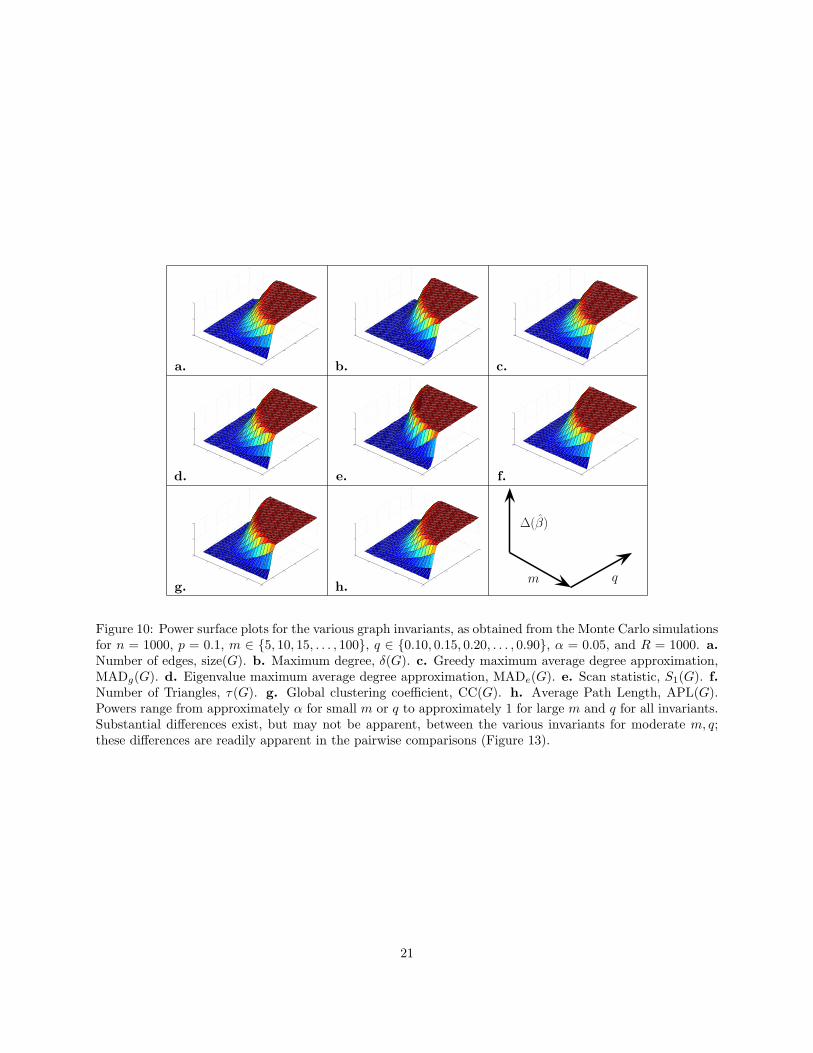
The power surface plots for the invariants are superficially similar to one another, which makes deter-

mining the relative effectiveness of each invariant difficult. Powers for all invariants range from β ≈ α for

small m or q to β ≈ 1 for large m and q. Substantial differences exist, but may not be apparent, between

the various invariants for moderate m, q.

4.2 Power Difference Plots

In order to better analyze the comparative statistical power of our invariants, we examine the difference

between pairs of statistical power surfaces. These plots allow comparative power analyses across ΘA.

For many pairs of invariants, there exists a range of m and q for which each of the two invariants has

a higher power; neither invariant has greater power over all of ΘA. However, Figure 11 demonstrates that

S1(G) dominates δ(G), rendering the latter “inadmissible”. (This inadmissibility claim is supported by the

16

Monte Carlo results of Figure 11 for H0 : ER(n = 1000, p = 0.1) vs. HA : κ(n = 1000, p = 0.1,m, q)

only. However, the scan statistic is specifically designed to improve upon maximum degree for “chatter”

alternatives of the type represented by our κ random graph model, and we conjecture that this domination

holds more generally. An asymptotic version of this result is available (Rukhin and Priebe 2009).) Figure

12 demonstrates, again for H0 : ER(n = 1000, p = 0.1) vs. HA : κ(n = 1000, p = 0.1,m, q), that size(G) and

APL(G) are indistinguishable in terms of power over all of ΘA.

The comparative power surface plots shown in Figure 13 provide pairwise comparison of the remaining

four invariants, excluding the inadmissible δ(G) and including size(G) but not the then-superfluous APL(G).

Since powers are approximately α for small m or q and approximately 1 for large m and q for all invari-

ants, power differences are approximately 0 for these extremes. Substantial differences are readily apparent

between the various invariants for moderate m and q in these comparative power surfaces. No invariant

dominates any other over all of ΘA. Figure 14 presents in more detail the interesting case of S1(G) vs. τ(G).

When m is large and q is small βτ(G) > βS1(G), while when m is small and q is large βS1(G) > βτ(G), and the

power differences are large in both cases. Neither invariant dominates the other throughout ΘA.

4.3 Most Powerful Statistic

When the power of all the invariants are examined together, the range of values for m and q for which each

has the greatest power is shown in Figure 15a. Only S1(G), CC(G), and τ(G) show best power at least

somewhere in ΘA. The scan statistic S1(G) is best for moderate m, q; CC(G) dominates when m is small

and q is large; and τ(G) dominates for large m and small q.

We have presented detailed results for (m, q) ∈ ΘA, but for just one choice of n, p – n = 1000, p = 0.1.

Figures 15b and 15c present “most powerful statistic over ΘA”, analogous to Figure 15a, for other choices

of n, p. In the case n = 100, p = 0.1 we see S1(G) as dominate for the large q small m region and MADe(G)

as dominate for the small q large m region. (Notice that we consider m much larger as a percentage of n in

Figures 15b and 15c.) For the case n = 100, p = 0.4 the clustering coefficient CC(G) dominates. Some of

the smattering effects in these figures is due to artifacts of the Monte Carlo; the basic structure of the plots

is real. The fundamental result is that there does not necessarily exist a single uniformly most powerful

statistic, across all of ΘA.

We have performed extensive Monte Carlo Analysis generalizing Figure 15 for numerous n, p cases. The

suggestive results seen in Figure 15 seem to hold generally: the scan statistic and the clustering coefficient

are often most powerful, and τ(G) and MADe(G) occasionally come into play; rarely if ever are the other

invariants recommended.

17

5 Conclusions

Analytics are preferable to Monte Carlo. However, finite-sample comparative power analytics for random

graphs are challenging even in this relatively simple setting, and asymptotic analytics can be at odds with

finite sample truths even for extraordinarily large n (Rukhin and Priebe 2009). The snapshots into compar-

ative test behavior available via Monte Carlo analysis provide new and valuable understanding for statistical

inference on random graphs, and will form the foundation for comparative power investigations for larger

graphs and more complex models.

From the statistical power surface plots, we observe that all the graph invariants we examined have

power β ≈ 1 for large m and q and power β ≈ α for small m or q, as expected. For moderate m and

q, the comparative behavior of the various invariants is quite complicated; different invariants dominate in

different regions. In particular, there is in general a ridge/trough phenomenon running (nonlinearly) from

large q small m to small q large m which seems to differentiate invariants – some invariants are recommended

in the small q large m region and others are recommended in the large q small m region. There does not

exist a uniformly most powerful statistic across all of ΘA. That is, the specific alternative – how many

anomalous vertices (m) and by how much are they anomalous (q) – determines the most powerful statistic.

If a recommendation is required, without knowledge of the specific alternative m, q, we suggest (based on

Figure 13 and related results) using scan statistic and clustering coefficient together, since the best of those

two is rarely out-performed by much but there exists regions of ΘA where each out-performs the other

substantially. This requires two tests, and multiple-testing correction, but if no information is available

regarding m and q then this seems a good course of action.

The “statistical inference on random graphs” considered herein is hypothesis testing. Of course, once

one rejects in favor of κ(n, p,m, q), the question of estimating m and q, as well as identifying the anomalous

vertex set VA, naturally arises. The more general inferential tasks are of substantial interest, but involve

complicating issues best addressed after gaining solid understanding from our simpler comparative power

analysis. For instance: we have treated p as known throughout this manuscript. Treating p as unknown

both is more realistic and presents a confounding issue. Consideration of estimating p under HA begins with

assuming the anomalous m vertices are known – that is, we know the set VA. Then

p = size(Ω(V \ VA))/(n−m

2

).

Thus the problem is to find VA. One approach is to let VA = N [v∗] – that is, the vertex of maximum

degree or maximum locality statistic size(Ω(N1[v])) together with all its neighbors. This is a reasonable first

estimator for p (and |N [v∗]| and size(Ω(N1[v∗]))/(|N [v∗]|

2

)provide reasonable estimators for m and q). There

are, however, many potential improvements available regarding the estimation of p, involving resampling or

18

iteration or bias correction based on asymptotic alternative distribution moments. In any event, we see that

estimating p requires identifying VA, which is clearly harder than the testing problem considered herein.

Thus, while it is true that power analyses are affected by unknown p, we feel that full-scale consideration of

this issue at this time would obscure the simpler, basic comparative power issues which can be elucidated

by considering known p.

In summation, no one invariant is uniformly most powerful at detecting increases in local “chatter”;

even in this relatively simple setting, our investigation suggests that finite sample statistical inference on

random graphs poses significant complexities. Our Monte Carlo investigation provides useful insight into

the comparative behavior of various invariants.

6 Acknowledgements

The authors thank Andrey Rukhin for assistance regarding invariant distributions, and three referees for

insightful comments which were instrumental in improving this manuscript.

7 Supplemental Materials

Code for reproducing all the simulation results presented in this paper is available at

http://www.glencoppersmith.com/code/.

References

Bickel, P. and Doksum, K. (2001), Mathematical statistics, Prentice Hall Upper Saddle River, NJ.

Bollobas, B. (2001), Random Graphs, Cambridge University Press.

Doddington, G., Mitchell, A., Przybocki, M., Ramshaw, L., Strassel, S., and Weischedel, R. (2004), “The

Automatic Content Extraction (ACE) Program Tasks, Data, and Evaluation,” In Proceedings LREC,

pages 837–840.

Grothendieck, J., Gorin, A., and Borges, N. (2008), “Social Correlates of Turn-taking Behavior,” in prepa-

ration.

Horn, R. and Johnson, C. (1985), Matrix Analysis, Cambridge University Press.

Leenders, R. (1995), Structure and influence: Statistical models for the dynamics of actor attributes, network

structure, and their interdependence, Thesis Publishers.

19

Newman, M.E.J. (2003), “The Structure and Function of Complex Networks,” SIAM Review, 45(2):167–256.

Newman, M.E.J., Barabosi, A.-L., and Watts, D.J. (2006), The Structure and Dynamics of Networks,

Princeton: Princeton University Press.

Nowicki, K. and Wierman, J. (1988), “Subgraph Counts in Random Graphs Using Incomplete UStatistics

Methods,” Discrete Mathematics, 72:299–310.

Priebe, C., Conroy, J., Marchette, D., and Park, Y. (2005), “Scan Statistics on Enron Graphs,” Computa-

tional & Mathematical Organization Theory, 11(3):229–247.

Rukhin, A. (2008), Asymptotic Analysis of Various Statistics for Random Graph Inference, PhD thesis,

Department of Applied Math and Statistics Dissertation, Johns Hopkins University.

Rukhin, A. and Priebe, C.E. (2009a), “On the Limiting Distribution of a Graph Scan Statistic,” submitted

for publication.

Rukhin, A. and Priebe, C.E. (2009b), “A Comparative Power Analysis of the Maximum Degree and Size

Invariants for Random Graph Inference,” submitted for publication.

Sen, S., Spatschek, O., and Wang, D. (2004), “Accurate, Scalable In-network Identification of P2P Traffic

Using Application Signatures,” In Proceedings WWW’04, pages 512–521.

Ullman, D. and Scheinerman, E. (1997), Fractional Graph Theory, Wiley.

West, D. (2001), Introduction to Graph Theory, Prentice Hall Upper Saddle River, NJ, second edition.

20

a. b. c.

d. e. f.

g. h.m q

∆(β)

1

Figure 10: Power surface plots for the various graph invariants, as obtained from the Monte Carlo simulationsfor n = 1000, p = 0.1, m ∈ 5, 10, 15, . . . , 100, q ∈ 0.10, 0.15, 0.20, . . . , 0.90, α = 0.05, and R = 1000. a.Number of edges, size(G). b. Maximum degree, δ(G). c. Greedy maximum average degree approximation,MADg(G). d. Eigenvalue maximum average degree approximation, MADe(G). e. Scan statistic, S1(G). f.Number of Triangles, τ(G). g. Global clustering coefficient, CC(G). h. Average Path Length, APL(G).Powers range from approximately α for small m or q to approximately 1 for large m and q for all invariants.Substantial differences exist, but may not be apparent, between the various invariants for moderate m, q;these differences are readily apparent in the pairwise comparisons (Figure 13).

21

020

4060

80100 0

0.2

0.4

0.6

0.8

1−1

−0.5

0

0.5

1

qm

∆(β)

Figure 11: Comparative power surface for βδ(G) − βS1(G) for H0 : ER(n = 1000, p = 0.1) vs. HA : κ(n =1000, p = 0.1,m, q) for the range of m, q investigated. S1(G) has equal or superior power to δ(G) for all ofΘA.

020

4060

80100 0

0.20.4

0.60.8

1−1

−0.5

0

0.5

1

qm

∆(β)

Figure 12: Comparative power surface for βsize(G) − βAPL(G) for H0 : ER(n = 1000, p = 0.1) vs. HA :κ(n = 1000, p = 0.1,m, q) for the range of m, q investigated. The statistics size(G) and APL(G) have nearlyidentical power for all of ΘA.

22

MADe(G) S1(G) τ(G) CC(G)

size(G)

MADe(G)

S1(G)

τ(G) m q

∆(β)

1

Figure 13: Comparative power surfaces for the various graph invariants, as obtained from Monte Carlosimulations for n = 1000, p = 0.1, m ∈ 5, 10, 15, . . . , 100, q ∈ 0.10, 0.15, 0.20, . . . , 0.90, α = 0.05, andR = 1000. Each surface plot is representative of the power of the row invariant minus the power of thecolumn invariant (e.g. the upper left corner depicts βsize(G) − βMADe(G)) from Figure 10. Since powersare approximately α for small m or q and approximately 1 for large m and q for all invariants, powerdifferences are approximately 0 in these regions. Substantial differences are readily apparent between thevarious invariants for moderate m, q in these comparative power surfaces. This phenomenon can be seen inmore detail in Figure 14.

23

020

4060

80100 0

0.20.4

0.60.8

1−1

−0.5

0

0.5

1

qm

∆(β)

Figure 14: Comparative power surface βS1(G) − βτ(G) for H0 : ER(1000, 0.1) vs. HA : κ(1000, 0.1,m, q) withα = 0.05 andR = 1000, from Figure 13. Since powers are approximately α for smallm or q and approximately1 for large m and q for both invariants, power differences are approximately 0 in these regions. Substantialdifferences are readily apparent for moderate m, q: when m is large and q is small βτ(G) > βS1(G); when m

is small and q is large βS1(G) > βτ(G). Neither invariant dominates the other throughout ΘA.

24

a. m

q

10 20 30 40 50 60 70 80 90 100

0.1

0.2

0.3

0.4

0.5

0.6

0.7

0.8

0.9

1

CC

!

S1

b. m

q

5 10 15 20 25 30 35 40

0.1

0.2

0.3

0.4

0.5

0.6

0.7

0.8

0.9

1

MADg

!

S1

MADe

c.m

q

5 10 15 20 25 30 35 40

0.4

0.5

0.6

0.7

0.8

0.9

1

S1

CC

Figure 15: Most powerful statistic over ΘA for selected n and p for H0 : ER(n, p) vs. HA : κ(n, p,m, q) withα = 0.05 and R = 1000. The dark blue region is where no test is statistically significantly superior. For largem and q (relative to n and p), this is because all tests have β ≈ 1; for small m or small q, this is because alltests have β ≈ α. a. n = 1000, p = 0.1, m ∈ 5, 10, 15, . . . , 100, q ∈ 0.10, 0.15, 0.20, . . . , 1.0 as in Figures10 and 13. b. n = 100, p = 0.1, m ∈ 2, 4, 6, . . . , 40, q ∈ 0.10, 0.15, 0.20, . . . , 1.0. c. n = 100, p = 0.4,m ∈ 2, 4, 6, . . . , 40, q ∈ 0.40, 0.45, 0.50, . . . , 1.0.

25