Entropy Statistics Tests Goodness of Fit Wald Lagrange Likelihood Ratio

Quantitative Economics 12 (2021), 683–742 1759-7331/20210683
Specification tests for non-Gaussian maximum likelihoodestimators
Gabriele FiorentiniDepartment of Statistics, Informatics and Applications, Università di Firenze and RCEA
Enrique SentanaCEMFI
We propose generalized DWH specification tests which simultaneously com-pare three or more likelihood-based estimators in multivariate conditionally het-eroskedastic dynamic regression models. Our tests are useful for Garch mod-els and in many empirically relevant macro and finance applications involvingVars and multivariate regressions. We determine the rank of the differences be-tween the estimators’ asymptotic covariance matrices under correct specification,and take into account that some parameters remain consistently estimated underdistributional misspecification. We provide finite sample results through MonteCarlo simulations. Finally, we analyze a structural Var proposed to capture therelationship between macroeconomic and financial uncertainty and the businesscycle.
Keywords. Durbin–Wu–Hausman tests, partial adaptivity, semiparametric esti-mators, singular covariance matrices, uncertainty and the business cycle.
JEL classification. C12, C14, C22, C32, C52.
1. Introduction
Empirical studies with financial data suggest that returns distributions are leptokurticeven after controlling for volatility clustering effects. This feature has important prac-tical consequences for standard risk management measures such as Value at Risk andrecently proposed systemic risk measures such as Conditional Value at Risk or Marginal
Gabriele Fiorentini: [email protected] Sentana: [email protected] paper draws heavily on Fiorentini and Sentana (2007). In addition to those explicitly acknowledgedthere, we would like to thank Dante Amengual, Christian Bontemps and Luca Fanelli for useful commentsand suggestions, as well as audiences at CREST, Konstanz, Tokyo, UCLA, UCSD, the University of Liverpool6th Annual Econometrics Workshop (April 2017), the University of Southampton Finance and EconometricsWorkshop (May 2017), the SanFI conference on “New Methods for the Empirical Analysis of Financial Mar-kets” (Comillas, June 2017), the 70th ESEM (Lisbon, August 2017), the Bilgi CEFIS conference on “Advancesin Econometrics Methods” (Instanbul, March 2018), the Financial Engineering and Risk Management Con-ference (Shanghai, June 2018), the University of Kent “50 Years of Econometrics at Keynes College” Con-ference (Canterbury, September 2018), and the TSE Financial Econometrics Conference (Toulouse, May2019). The coeditor and two anonymous referees have provided very useful feedback. Of course, the usualcaveat applies. The second author acknowledges financial support from the Spanish Ministry of Economy,Industry and Competitiveness through grant ECO 2017-89689 and the Santander CEMFI Research Chair.
© 2021 The Authors. Licensed under the Creative Commons Attribution-NonCommercial License 4.0.Available at http://qeconomics.org. https://doi.org/10.3982/QE1406

684 Fiorentini and Sentana Quantitative Economics 12 (2021)
Expected Shortfall (see Adrian and Brunnermeier (2016) and Acharya, Pedersen, Philip-pon, and Richardson (2017), respectively), which could be severely mismeasured by as-suming normality. Given that empirical researchers are interested in those risk measuresfor several probability levels, they often specify a parametric leptokurtic distribution,which then they use to estimate their models by maximum likelihood (ML).
A nontrivial by-product of these non-Gaussian ML procedures is that they delivermore efficient estimators of the mean and variance parameters, especially if the shapeparameters can be fixed to their true values. The downside, though, is that they oftenachieve those efficiency gains under correct specification at the risk of returning incon-sistent parameter estimators under distributional misspecification (see, e.g., Newey andSteigerwald (1997)). This is in marked contrast with the generally inefficient Gaussianpseudo-maximum likelihood (PML) estimators advocated by Bollerslev and Wooldridge(1992) among many others, which remain root-T consistent for the mean and varianceparameters under relatively weak conditions.
If researchers were only interested in those two conditional moments, the semi-parametric (SP) estimators of Engle and Gonzalez-Rivera (1991) and Gonzalez-Riveraand Drost (1999) would provide an attractive solution because they are consistent andalso attain full efficiency for a subset of the parameters (see Linton (1993), Drost andKlaassen (1997), Drost, Klaassen, and Werker (1997), and Sun and Stengos (2006) forunivariate time series examples). Unfortunately, SP estimators suffer from the curse ofdimensionality when the number of series involved, N , is moderately large, which limitstheir use. Furthermore, Amengual, Fiorentini, and Sentana (2013) show that nonpara-metrically estimated conditional quantiles lead to risk measures with much wider confi-dence intervals than their parametric counterparts even in univariate contexts. Anotherpossibility would be the spherically symmetric semiparametric (SSP) methods consid-ered by Hodgson and Vorkink (2003) and Hafner and Rombouts (2007), which are alsopartially efficient while retaining univariate rates for their nonparametric part regard-less of N . However, asymmetries in the true joint distribution will contaminate theseestimators too.
In any event, given that many research economists at central banks, financial institu-tions, and economic consulting firms continue to rely on the estimators that commer-cial econometric software packages provide, it would be desirable that they routinelycomplemented their empirical results with some formal indication of the validity of theparametric assumptions they make.
The statistical and econometric literature on model specification is huge. In this pa-per, our focus is the adequacy of the conditional distribution under the maintained as-sumption that the rest of the model is correctly specified. Even so, there are various waysof assessing it. One possibility is to nest the assumed distribution within a more flexibleparametric family in order to conduct a Lagrange Multiplier (LM) test of the nesting re-strictions. This is the approach in Mencía and Sentana (2012), who use the generalizedhyperbolic family as an instrumental nesting distribution for the multivariate Student t.In contrast, other specification tests do not consider an explicit alternative hypothesis.A case in point are consistent tests based on the difference between the theoretical andempirical cumulative distribution functions of the innovations (Bai (2003) and Bai and

Quantitative Economics 12 (2021) Specification tests for non-Gaussian ML estimators 685
Zhihong (2008)) or their characteristic functions (Bierens and Wang (2012) and Amen-gual, Carrasco, and Sentana (2020)). An alternative procedure would be the informationmatrix test of White (1982), which compares some or all of the elements of the expectedHessian and the variance of the score. White (1987) also proposed the application ofNewey’s (1985) conditional moment test to assesses the martingale difference propertyof the scores under correct specification. Finally, the general class of moment tests inNewey (1985) and Tauchen (1985) could also be entertained, as Bontemps and Meddahi(2012) illustrate.
But when a research economist relies on standard software for calculating somenon-Gaussian estimators of θ and their asymptotic standard errors from real data, amore natural approach to testing distributional specification would be to compare thoseestimators on a pairwise basis using simple Durbin–Wu–Hausman (DWH) tests.1 As iswell known, the traditional version of these tests can refute the correct specification of amodel by exploiting the diverging properties under misspecification of a pair of estima-tors of the same parameters. Focusing on the model parameters makes sense because ifthey are inconsistently estimated, the conditional moments derived from them will beinconsistently estimated too.
In this paper, we take this idea one step further and propose an extension of theDWH tests which simultaneously compares three or more estimators. The rationale forour proposal is given by a novel proposition which shows that if we order the five esti-mators we mentioned in the preceding paragraphs as restricted and unrestricted non-Gaussian ML, SSP, SP, and Gaussian PML, each estimator is “efficient” relative to all theothers behind. This “Matryoshka doll” structure for their joint asymptotic covariancematrix implies that there are four asymptotically independent contiguous comparisons,and that any other pairwise comparison must be a linear combination of those four. Weexploit these properties in developing the asymptotic distribution of our proposed mul-tiple comparison tests. We also explore several important issues related to the practicalimplementation of DWH tests, including its two score versions, their numerical invari-ance to reparametrizations, and their application to subsets of parameters.
To design reliable tests, we first need to figure out the rank of the difference betweenthe asymptotic covariance matrices under the null of correct specification so as to usethe right number of degrees of freedom. We also need to take into account that some pa-rameters continue to be consistently estimated under the alternative of incorrect distri-butional specification, thereby avoiding wasting degrees of freedom without providingany power gains.
In Fiorentini and Sentana (2019), we characterized the mean and variance parame-ters that distributionally misspecified ML estimators can consistently estimate, and pro-vided simple closed-form consistent estimators for the rest. One of the most interestingresults that we obtain in this paper is that the parameters that continue to be consis-tently estimated by the parametric estimators under distributional misspecification arethose which are efficiently estimated by the semiparametric procedures. In contrast, the
1Wu (1973) compared OLS with IV in linear single equation models to assess regressor exogeneity un-aware that Durbin (1954) had already suggested this. Hausman (1978) provided a procedure with far widerapplicability.

686 Fiorentini and Sentana Quantitative Economics 12 (2021)
remaining parameters, which will be inconsistently estimated by distributionally mis-specified parametric procedures, the semiparametric procedures can only estimate withthe efficiency of the Gaussian PML estimator. Therefore, we will focus our tests on thecomparison of the estimators of this second group of parameters, for which the usualefficiency—consistency trade off is of first-order importance.
The inclusion of means and the explicit coverage of multivariate models make ourproposed tests useful not only for Garch models but also for dynamic linear mod-els such as Vars or multivariate regressions, which remain the workhorse in empiri-cal macroeconomics and asset pricing contexts. This is particularly relevant in prac-tice because researchers are increasingly acknowledging the nonnormality of manymacroeconomic variables (see Lanne, Meitz, and Saikkonen (2017) and the referencestherein for recent examples of univariate and multivariate time series models with non-Gaussian innovations). Nevertheless, structural models pose some additional inferencechallenges, which we discuss separately. Obviously, our approach also applies in cross-sectional models with exogenous regressors, as well as in static ones.
The rest of the paper is as follows. In Section 2, we provide a quick revision of DWHtests and derive several new results which we use in our subsequent analysis. Then, inSection 3 we formally present the five different likelihood-based estimators that we havementioned, and derive our proposed specification tests, paying particular attention totheir degrees of freedom and power. A Monte Carlo evaluation of our tests can be foundin Section 4, followed by an empirical analysis of the relationship between uncertaintyand the business cycle using a structural Var. Finally, we present our conclusions inSection 6. Proofs and auxiliary results are gathered in Appendices.
2. Durbin–Wu–Hausman tests
2.1 Wald and score versions
Let θT and θT denote two GMM estimators of θ based on the average influence func-tions mT (θ) and nT (θ) and weighting matrices SmT and SnT , respectively. When bothsets of moment conditions hold, then under standard regularity conditions (see, e.g.,Newey and McFadden (1994)), the estimators will be jointly root-T consistent andasymptotically Gaussian, so
√T(θT − θT ) d→ N(0�Δ) and
T(θT − θT )′Δ−(θT − θT ) d→ χ2r � (1)
where r = rank(Δ) and − denotes a generalized inverse. Consider now a sequence oflocal alternatives such that
√T(θT − θT ) ∼ N(θm − θn�Δ)� (2)
In this case, the asymptotic distribution of the DWH statistics (1) will become a non-central chi-square with noncentrality parameter (θm − θn)′Δ−(θm − θn) and the samenumber of degrees freedom (see, e.g., Hausman (1978) or Holly (1987)). Therefore, the

Quantitative Economics 12 (2021) Specification tests for non-Gaussian ML estimators 687
local power of a DWH test will be increasing in the limiting discrepancy between the twoestimators, and decreasing in both the number and magnitude of the nonzero eigenval-ues of Δ.
Knowing the right number of degrees of freedom is particularly important for em-ploying the correct distribution under the null. Unfortunately, some obvious consistentestimators ofΔmight lead to inconsistent estimators ofΔ−.2 In fact, they might not evenbe positive semidefinite in finite samples. We will revisit these issues in Sections 3.4 and3.6, respectively.
The calculation of the DWH test statistic (1) requires the prior computation of θTand θT . In a likelihood context, however, Theorem 5.2 of White (1982) implies that anasymptotically equivalent test can be obtained by evaluating the scores of the restrictedmodel at the inefficient but consistent parameter estimator (see also Reiss (1983) andRuud (1984), as well as Davidson and MacKinnon (1989)). Theorem 2.5 in Newey (1985)shows that the same equivalence holds in situations in which the estimators are definedby moment conditions. In fact, it is possible to derive not just one but two asymptoticallyequivalent score versions of the DWH test by evaluating the influence functions that giverise to each of the estimators at the other estimator, as explained in Section 10.3 of White(1994). The following proposition, which we include for completeness, spells out thoseequivalences:
Proposition 1. Assume that the moment conditions mt (θ) and nt (θ) are correctly spec-ified. Then, under standard regularity conditions,
T(θT − θT )′Δ−(θT − θT )− Tm′T (θT )SmJm(θ0)Λ
−mJ ′
m(θ0)SmmT (θT ) = op(1) and (3)
T(θT − θT )′Δ−(θT − θT )− T n′T (θT )SnJn(θ0)Λ
−n J ′
n(θ0)SnnT (θT ) = op(1)� (4)
where Λm and Λn are, respectively, the limiting variances of J ′m(θ0)Sm
√TmT (θT ) and
J ′n(θ0)Sn
√T nT (θT ), which are such that
Δ= [J ′m(θ0)SmJm(θ0)
]−1Λm
[J ′m(θ0)SmJm(θ0)
]−1
= [J ′n(θ0)SnJn(θ0)
]−1Λn[J ′n(θ0)SnJn(θ0)
]−1
with Jm(θ) = plimT→∞ ∂mT (θ)/∂θ′, Jn(θ) = plimT→∞ ∂nT (θ)/∂θ
′, Sm = plimT→∞ SmT ,Sn = plimT→∞ SnT and rank[J ′
m(θ0)SmJm(θ0)] = rank[J ′n(θ0)SnJn(θ0)] = p = dim(θ), so
that rank(Λm) = rank(Λn) = rank(Δ).
An intuitive way of reinterpreting the asymptotic equivalence between the orig-inal DWH test in (1) and the two alternative score versions on the right-hand sidesof (3) and (4) is to think of the latter as original DWH tests based on two conve-nient reparametrizations of θ obtained through the population version of the first or-der conditions that give rise to each estimator, namely πm(θ) = J ′
m(θ)SmE[mt (θ)] and
2A trivial nonrandom example of discontinuities is the sequence 1/T , which converges to 0 while itsgeneralized inverse (1/T)− = T diverges. Theorem 1 in Andrews (1987) provides conditions under which aquadratic form based on a generalized inverse of a weighting matrix converges to a chi-square distribution.

688 Fiorentini and Sentana Quantitative Economics 12 (2021)
πn(θ) = J ′n(θ)SnE[nt (θ)]. While these new parameters are equal to 0 when evaluated
at the pseudo-true values of θ implicitly defined by the exactly identified moment con-ditions J ′
m(θm)SmE[mt(θm)] = 0 and J ′n(θn)SnE[nt(θn)] = 0, respectively, πm(θn) and
πn(θm) are not necessarily so, unless the correct specification condition θm = θn = θ0
holds.3 The same arguments also allow us to loosely interpret the score versions of theDWH tests as distance metric tests of those moment conditions, as they compare thevalues of the GMM criteria at the estimator which sets those exactly identified momentsto 0 with their values at the alternative estimator. We will discuss more formal links to theclassical Wald, Likelihood Ratio (LR) and LM tests in a likelihood context in Section 3.4.
Proposition 1 implies the choice between the three versions of the DWH test mustbe based on either computational ease, numerical invariance or finite sample reliability.While computational ease is model specific, we will revisit the last two issues in Sec-tions 2.2 and 4, respectively.
2.2 Numerical invariance to reparametrizations
Suppose we decide to work with an alternative parametrization of the model for con-venience or ease of interpretation. For example, we might decide to compare the logsof the estimators of a variance parameter rather than their levels. We can then state thefollowing result.
Proposition 2. Consider a homeomorphic, continuously differentiable transforma-tion π(·) from θ to a new set of parameters π, with rank[∂π ′(θ)/∂θ] = p = dim(θ)
when evaluated at θ0, θT , and θT . Let πT = arg minπ∈Π m′T (π)SmT mT (π) and πT =
arg minπ∈Π n′T (π)SnT nT (π), where mt (π) = mt[θ(π)] and nt (π)= nt[θ(π)] are the influ-
ence functions written in terms of π, with θ(π) denoting the inverse mapping such thatπ[θ(π)] =π. Then:
1. The Wald versions of the DWH tests based on θT − θT and πT − πT are numeri-cally identical if the mapping is affine, so that π = Aθ+ b, with A and b known and|A| �= 0.
2. The score versions of the tests based on mT (θT ) and mT (πT ) are numerically identi-cal if
Λ∼mT =
[∂θ(πT )
∂π ′]−1
Λ∼mt
[∂θ′(πT )
∂π
]−1�
whereΛ∼mT andΛ∼
mT , are consistent estimators of the generalized inverses of the lim-iting variances of J ′
m(θ0)Sm
√TmT (θT ) and J ′
m(θ0)Sm
√T mT (πT ), respectively.
3. An analogous result applies to the score versions based on nT (θT ) and nT (πT ).
3A related analogy arises in indirect estimation, in which the asymptotic equivalence between the score-based methods proposed by Gallant and Tauchen (1996) and the parameter-based methods in Gouriéroux,Monfort, and Renault (1993) can be intuitively understood if we regard the expected values of the scores ofthe auxiliary model as a new set of auxiliary parameters that summarizes all the information in the originalparameters (see Calzolari, Fiorentini, and Sentana (2004) for further details and a generalization).

Quantitative Economics 12 (2021) Specification tests for non-Gaussian ML estimators 689
These numerical invariance results, which extend those in Sections 17.4 and 22.1 ofRuud (2000), suggest that the score-based tests might be better behaved in finite sam-ples than their “Wald” counterpart. We will provide some simulation evidence on thisconjecture in Section 4.
2.3 Subsets of parameters
In some examples, generalized inverses can be avoided by working with a parametersubvector. In particular, if the (scaled) difference between two estimators of the last p2elements of θ, θ2T , and θ2T , converge in probability to 0, then comparing θ1T and θ1T isanalogous to using a generalized inverse with the entire parameter vector (see Holly andMonfort (1986) for further details).
But one may also want to focus on a subset if the means of the asymptotic distribu-tions of θ2T and θ2T coincide both under the null and the alternative, so that a DWH testinvolving these parameters will result in a waste of degrees of freedom, and thereby aloss of power.
The following result provides a useful interpretation of the two score versionsasymptotically equivalent to a Wald-style DWH test that compares θ1T and θ1T .
Proposition 3. Define
m⊥1T (θ�Sn) = J ′
1m(θ)SmmT (θ)
−J ′1m(θ)SmJ2m(θ)
[J ′
2m(θ)SmJ2m(θ)]−1J ′
2m(θ)SmmT (θ)�
n⊥1T (θ�Sn) = J ′
1n(θ)SnnT (θ)−J ′1n(θ)SnJ2n(θ)
[J ′
2n(θ)SnJ2n(θ)]−1J ′
2n(θ)SnnT (θ)
as two sets of p1 transformed sample moment conditions, where
Jm(θ) =[J1m(θ) J2m(θ)
]=[
plimT→∞
∂mT (θ)/∂θ′1 plim
T→∞∂mT (θ)/∂θ
′2]�
Jn(θ) =[J1n(θ) J2n(θ)
]=[
plimT→∞
∂nT (θ)/∂θ′1 plim
T→∞∂nT (θ)/∂θ
′2]�
If mt (θ) and nt (θ) are correctly specified, then under standard regularity conditions,
T(θT − θT )′Δ−11(θT − θT )− Tm⊥′
T (θT )Λ−m⊥
1m⊥′
T (θT ) = op(1) and
T(θ1T − θ1T )′Δ−
11(θ1T − θ1T )− T n⊥′1T (θT )Λ
−n⊥
1n⊥
1T (θT ) = op(1)�
where Δ11, Λm⊥1
and Λn⊥1
are the limiting variances of√T(θ1T − θ1T ),
√Tm⊥
1T (θT �Sm)
and√T n⊥
1T (θT �Sn), respectively, which are such that
Δ11 = [J ′m(θ0)SmJm(θ0)
]11Λm⊥
1
[J ′m(θ0)SmJm(θ0)
]11
= [J ′n(θ0)SnJn(θ0)
]11Λn⊥
1
[J ′n(θ0)SnJn(θ0)
]11�
with 11 denoting the diagonal block of the relevant inverse corresponding to θ1.

690 Fiorentini and Sentana Quantitative Economics 12 (2021)
Intuitively, we can understand m⊥1T (θ�Sn) and n⊥
1T (θ�Sn) as moment conditions thatexactly identify θ1, but with the peculiarity that
plimT→∞
∂m⊥1T (θ�Sn)
∂θ′2
= plimT→∞
∂n⊥1T (θ�Sn)
∂θ′2
= 0�
which makes them asymptotically immune to the sample variability in the estimatorsof θ2.
When J ′1m(θ)SmJ2m(θ) = J ′
1n(θ)SnJ2n(θ) = 0, the above moment tests will beasymptotically equivalent to tests based on J ′
1m(θ)Sm
√TmT (θT ) and J ′
1n(θ)Sn
√T ×
nT (θT ), respectively, but in general this will not be the case.
2.4 Multiple simultaneous comparisons
All applications of DWH tests we are aware of compare two estimators of the sameunderlying parameters. However, as we shall see in Section 3.2, there are situations inwhich three or more estimators are available. In those circumstances, it might not beentirely clear which pair of estimators researchers should focus on.
Ruud (1984) highlighted a special factorization structure of the likelihood such thatdifferent pairwise comparisons give rise to asymptotically equivalent tests. He illus-trated his result with three classical examples: (i) full sample versus first subsampleversus second subsample in Chow tests; (ii) GLS versus within-groups versus between-groups in panel data; and (iii) Tobit versus probit versus truncated regressions. Unfortu-nately, Ruud’s (1984) factorization structure does not apply in our case.
In general, the best pairwise comparison, in the sense of having maximum poweragainst a given sequence of local alternatives, would be the one with the highest non-centrality parameter among those tests with the same number of degrees of freedom.4
But in practice, a researcher might not be able to make the required calculations with-out knowing the nature of the departure from the null. In those circumstances, a sensi-ble solution would be to simultaneously compare all the alternative estimators. Such ageneralization of the DWH test is conceptually straightforward, but it requires the jointasymptotic distribution of the different estimators involved. There is one special case inwhich this simultaneous test takes a particularly simple form.
Proposition 4. Let θjT , j = 1� � � � � J denote an ordered sequence of asymptotically Gaus-
sian estimators of θwhose joint asymptotic covariance matrix adopts the following form:⎡⎢⎢⎢⎢⎢⎢⎣
Ω1 Ω1 � � � Ω1 Ω1
Ω1 Ω2 � � � Ω2 Ω2���
���� � �
������
Ω1 Ω2 � � � ΩJ−1 ΩJ−1
Ω1 Ω2 � � � ΩJ−1 ΩJ
⎤⎥⎥⎥⎥⎥⎥⎦� (5)
4Ranking tests with different degrees of freedom is also straightforward but more elaborate (see Holly(1987)).

Quantitative Economics 12 (2021) Specification tests for non-Gaussian ML estimators 691
The DWH test comparing all J estimators, T∑J
i=2(θjT − θj−1
T )′(Ωj −Ωj−1)+(θjT − θj−1
T ),is the sum of J − 1 consecutive pairwise DWH tests that are asymptotically mutually inde-pendent under the null of correct specification and sequences of local alternatives.
Hence, the asymptotic distribution of the simultaneous DWH test will be a noncen-tral χ2 with degrees of freedom and noncentrality parameters equal to the sum of the de-grees of freedom and noncentrality parameters of the consecutive pairwise DWH tests.Moreover, the asymptotic independence of the tests implies that in large samples, theprobability that at least one pairwise test will reject under the null will be 1 − (1 −α)J−1,where α is the common significance level.
Positive semidefiniteness of the covariance structure in (5) implies that one can rank(in the usual positive semidefinite sense) the asymptotic variance of the J estimators as
ΩJ ≥ΩJ−1 ≥ · · · ≥Ω2 ≥Ω1�
so that the sequence of estimators follows a decreasing efficiency order. Nevertheless,(5) goes beyond this ordering because it effectively implies that the estimators behavelike Matryoshka dolls, with each one being “efficient” relative to all the others below.Therefore, Proposition 4 provides the natural multiple comparison generalization ofLemma 2.1 in Hausman (1978).
An example of the covariance structure (5) arises in the context of sequential, gen-eral to specific tests of nested parametric restrictions (see Holly (1987) and Section 22.6of Ruud (2000)). More importantly for our purposes, the same structure also arises natu-rally in the comparison of parametric and semiparametric likelihood-based estimatorsof multivariate, conditionally heteroskedastic, dynamic regression models, to which weturn next.
3. Application to non-Gaussian likelihood estimators
3.1 Model specification
In a multivariate dynamic regression model with time-varying variances and covari-ances, the vector of N observed variables, yt , is typically assumed to be generated as
yt =μt (θ)+Σ1/2t (θ)ε∗
t �
where μt (θ) = μ(It−1;θ), Σt (θ) =Σ(It−1;θ), μ(·), and vech[Σ(·)] are N × 1 and N(N +1)/2 × 1 vector functions describing the conditional mean vector and covariance matrixknown up to the p × 1 vector of parameters θ, It−1 denotes the information set avail-able at t − 1, which contains past values of yt and possibly some contemporaneous
conditioning variables, and Σ1/2t (θ) is some particular “square root” matrix such that
Σ1/2t (θ)Σ
1/2′t (θ) = Σt (θ). Throughout the paper, we maintain the assumption that the
conditional mean and variance are correctly specified, in the sense that there is a truevalue of θ, say θ0, such that E(yt |It−1) = μt (θ0) and V (yt |It−1) =Σt (θ0). We also main-tain the high level regularity conditions in Bollerslev and Wooldridge (1992) because wewant to leave unspecified the conditional mean vector and covariance matrix in order

692 Fiorentini and Sentana Quantitative Economics 12 (2021)
to achieve full generality. Primitive conditions for specific multivariate models can befound, for example, in Ling and McAleer (2003).
To complete the model, a researcher needs to specify the conditional distributionof ε∗
t . In Supplemental Appendix D (Fiorentini and Sentana (2021)), we study the gen-eral case. In view of the options that the dominant commercially available econometricsoftware companies offer to their clients, though, in the main text we study the situa-tion in which a researcher makes the assumption that, conditional on It−1, the distribu-tion of ε∗
t is independent and identically distributed as some particular member of thespherical family with a well-defined density, or ε∗
t |It−1;θ�η∼ i�i�d� s(0� IN�η) for short,where η denotes q additional shape parameters which effectively characterize the distri-bution of ςt = ε∗′
t ε∗t (see Supplemental Appendix C for a brief introduction to spherically
symmetric distributions).5 The most prominent example is the standard multivariatenormal, which we denote by η = 0 without loss of generality. Another important ex-ample favored by empirical researchers is the standardized multivariate Student t withν degrees of freedom, or i�i�d� t(0� IN�ν) for short. As is well known, the multivariate t
approaches the multivariate normal as ν → ∞, but has generally fatter tails and allowsfor cross-sectional dependence beyond correlation. For tractability, we define η as 1/ν,which will always remain in the finite range [0�1/2) under our assumptions.6 Obviously,in the univariate case, any symmetric distribution, including the GED (also known asthe Generalized Gaussian distribution), is spherically symmetric, too.7
3.2 Likelihood-based estimators
Let LT (φ) denote the pseudo log-likelihood function of a sample of size T for the generalmodel discussed in Section 3.1, where φ= (θ′�η′)′ are the p+ q parameters of interest,which we assume variation-free. We consider up to five different estimators of θ.
1. Restricted ML (RML): θT (η), which is such that θT (η) = arg maxθ∈ΘLT (θ� η). Itsefficiency can be characterized by the θ, θ block of the information matrix, Iθθ(φ0), pro-vided that η= η0. Thus, we can interpret Iθθ(φ0) as the restricted parametric efficiencybound.
2. Joint or unrestricted ML (UML): θT , obtained as (θT � ηT ) = arg maxφ∈ΦLT (θ�η).In this case, P(φ0) = Iθθ(φ0) − Iθη(φ0)I−1
ηη(φ0)I ′θη(φ0) is the feasible parametric effi-
ciency bound.3. Spherically symmetric semiparametric (SSP): θT , which restricts ε∗
t to have an i�i�d�
s(0� IN�η) conditional distribution, but does not impose any additional structure on thedistribution of ςt = ε∗′
t ε∗t . This estimator is usually computed by means of one BHHH
iteration of the spherically symmetric efficient score starting from a consistent estimator
5Nevertheless, Propositions 10, 13, C2, D1, D2, and D3 already deal explicitly with the general case, whilePropositions 5, 6, 7, 8, and 9 continue to be valid without sphericity.
6A Student t with 1 < ν ≤ 2 implies an infinite variance, which is incompatible with the correct specifica-tion of Σt , while the conditional mean will not even be properly defined if ν ≤ 1.
7See McDonald and Newey (1988) for a univariate generalized t distribution, which nests both GED andStudent t, and Gillier (2005) for a spherically symmetric multivariate version of the GED.

Quantitative Economics 12 (2021) Specification tests for non-Gaussian ML estimators 693
(see Supplemental Appendix C.5 for further computational details).8 Associated to it wehave the spherically symmetric semiparametric efficiency bound S(φ0).
4. Unrestricted semiparametric (SP): θT , which only assumes that the conditionaldistribution of ε∗
t is i�i�d� (0� IN). It is also computed with one BHHH iteration of theefficient score starting from a consistent estimator (see Supplemental Appendix D.3 forfurther computational details). Associated to it we have the usual semiparametric effi-ciency bound S(φ0).
5. Gaussian pseudo ML (PML): θT = θT (0), which imposes η = 0 even though thetrue conditional distribution of ε∗
t might be neither normal nor spherical. As is wellknown, C−1(φ0) = A(φ0)B−1(φ0)A(φ0) gives the efficiency bound for this estimator,where A(φ0) is the expected Gaussian Hessian and B(φ0) the variance of the Gaussianscore.
Propositions C1–C3 in Supplemental Appendix C and Proposition D3 in Supplemen-tal Appendix D contain detailed expressions for all these efficiency bounds.
3.3 Covariance relationships
The next proposition provides the asymptotic covariance matrices of the different esti-mators presented in the previous section, and of the scores on which they are based:
Proposition 5. If ε∗t |It−1;φ0 is i�i�d� s(0� IN�η0) with bounded fourth moments, then
limT→∞
V
⎡⎢⎢⎢⎢⎢⎣
√T
T
T∑t=1
⎛⎜⎜⎜⎜⎜⎝
sθt (φ0)
sθ|ηt (φ0)
sθt (φ0)
sθt (φ0)
sθt (θ0�0)
⎞⎟⎟⎟⎟⎟⎠
⎤⎥⎥⎥⎥⎥⎦=
⎡⎢⎢⎢⎢⎢⎣
Iθθ(φ0) P(φ0) S(φ0) S(φ0) A(φ0)
P(φ0) P(φ0) S(φ0) S(φ0) A(φ0)
S(φ0) S(φ0) S(φ0) S(φ0) A(φ0)
S(φ0) S(φ0) S(φ0) S(φ0) A(φ0)
A(φ0) A(φ0) A(φ0) A(φ0) B(φ0)
⎤⎥⎥⎥⎥⎥⎦ (6)
and
limT→∞
V
⎡⎢⎢⎢⎢⎢⎣
√T
⎛⎜⎜⎜⎜⎜⎝
θT (η0)− θ0
θT − θ0
θT − θ0
θT − θ0
θT − θ0
⎞⎟⎟⎟⎟⎟⎠
⎤⎥⎥⎥⎥⎥⎦
=
⎡⎢⎢⎢⎢⎢⎣
I−1θθ (φ0) I−1
θθ (φ0) I−1θθ (φ0) I−1
θθ (φ0) I−1θθ (φ0)
I−1θθ (φ0) P−1(φ0) P−1(φ0) P−1(φ0) P−1(φ0)
I−1θθ (φ0) P−1(φ0) S−1(φ0) S−1(φ0) S−1(φ0)
I−1θθ (φ0) P−1(φ0) S−1(φ0) S−1(φ0) S−1(φ0)
I−1θθ (φ0) P−1(φ0) S−1(φ0) S−1(φ0) C(φ0)
⎤⎥⎥⎥⎥⎥⎦ � (7)
8Hodgson, Linton, and Vorkink (2002) also consider alternative estimators that iterate the semiparamet-ric adjustment until it becomes negligible. However, since they have the same first-order asymptotic distri-bution, we shall not discuss them separately.
694 Fiorentini and Sentana Quantitative Economics 12 (2021)
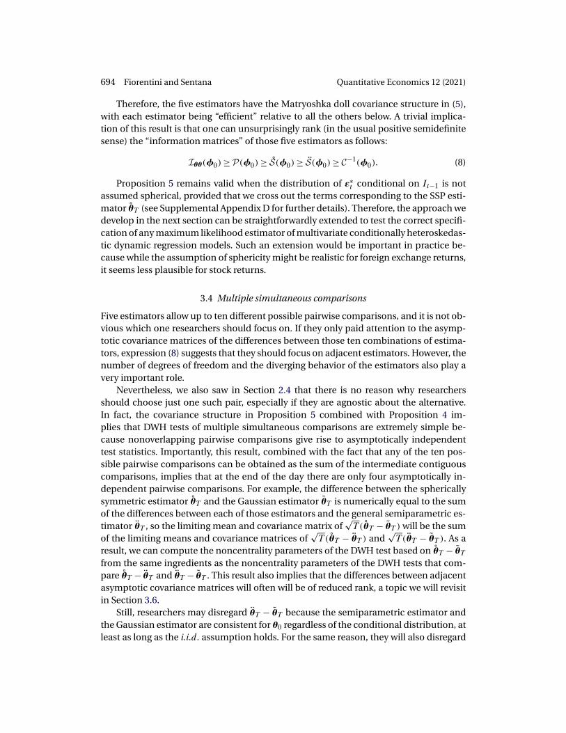
Therefore, the five estimators have the Matryoshka doll covariance structure in (5),with each estimator being “efficient” relative to all the others below. A trivial implica-tion of this result is that one can unsurprisingly rank (in the usual positive semidefinitesense) the “information matrices” of those five estimators as follows:
Iθθ(φ0) ≥ P(φ0) ≥ S(φ0) ≥ S(φ0) ≥ C−1(φ0)� (8)
Proposition 5 remains valid when the distribution of ε∗t conditional on It−1 is not
assumed spherical, provided that we cross out the terms corresponding to the SSP esti-mator θT (see Supplemental Appendix D for further details). Therefore, the approach wedevelop in the next section can be straightforwardly extended to test the correct specifi-cation of any maximum likelihood estimator of multivariate conditionally heteroskedas-tic dynamic regression models. Such an extension would be important in practice be-cause while the assumption of sphericity might be realistic for foreign exchange returns,it seems less plausible for stock returns.
3.4 Multiple simultaneous comparisons
Five estimators allow up to ten different possible pairwise comparisons, and it is not ob-vious which one researchers should focus on. If they only paid attention to the asymp-totic covariance matrices of the differences between those ten combinations of estima-tors, expression (8) suggests that they should focus on adjacent estimators. However, thenumber of degrees of freedom and the diverging behavior of the estimators also play avery important role.
Nevertheless, we also saw in Section 2.4 that there is no reason why researchersshould choose just one such pair, especially if they are agnostic about the alternative.In fact, the covariance structure in Proposition 5 combined with Proposition 4 im-plies that DWH tests of multiple simultaneous comparisons are extremely simple be-cause nonoverlapping pairwise comparisons give rise to asymptotically independenttest statistics. Importantly, this result, combined with the fact that any of the ten pos-sible pairwise comparisons can be obtained as the sum of the intermediate contiguouscomparisons, implies that at the end of the day there are only four asymptotically in-dependent pairwise comparisons. For example, the difference between the sphericallysymmetric estimator θT and the Gaussian estimator θT is numerically equal to the sumof the differences between each of those estimators and the general semiparametric es-timator θT , so the limiting mean and covariance matrix of
√T(θT − θT ) will be the sum
of the limiting means and covariance matrices of√T(θT − θT ) and
√T(θT − θT ). As a
result, we can compute the noncentrality parameters of the DWH test based on θT − θTfrom the same ingredients as the noncentrality parameters of the DWH tests that com-pare θT − θT and θT − θT . This result also implies that the differences between adjacentasymptotic covariance matrices will often will be of reduced rank, a topic we will revisitin Section 3.6.
Still, researchers may disregard θT − θT because the semiparametric estimator andthe Gaussian estimator are consistent for θ0 regardless of the conditional distribution, atleast as long as the i�i�d� assumption holds. For the same reason, they will also disregard

Quantitative Economics 12 (2021) Specification tests for non-Gaussian ML estimators 695
θT − θT if they maintain the assumption of sphericity. In practice, the main factor for de-ciding which estimators to compare is likely to be computational ease. For that reason,many empirical researchers might prefer to compare only the three parametric estima-tors included in standard software packages even though increases in power might beobtained under the maintained assumption of i�i�d� innovations by comparing θT to θTor θT instead of θT . The next proposition provides detailed expressions for the neces-sary ingredients of the three DWH test statistics in (1), (3), and (4) when we compare theunrestricted ML estimator of θ with its Gaussian PML counterpart.
Proposition 6. If the regularity conditions A.1 in Bollerslev and Wooldridge (1992) aresatisfied, then under the null of correct specification of the conditional distribution of yt
limT→∞
V[√
T(θT − θT )] = C(φ0)−P−1(φ0)�
limT→∞
V[√
T s′θ|ηT (θT �η0)
] = P(φ0)C(φ0)P(φ0)−P(φ0) and
limT→∞
V[√
T s′θT (θT �0)
] = B(φ0)−A(φ0)P−1(φ0)A(φ0)�
where sθ|ηT (θT �η0) is the sample average of the unrestricted parametric efficient score forθ evaluated at the Gaussian PML estimator θT , while sθT (θT �0) is the sample average ofthe Gaussian PML score evaluated at the unrestricted parametric ML estimator θT .
The next proposition provides the analogous expressions for the three DWH teststatistics in (1), (3), and (4) when we compare the restricted ML estimator of θ whichfixes η to η with its unrestricted counterpart, which simultaneously estimates these pa-rameters.
Proposition 7. If the regularity conditions in Crowder (1976) are satisfied, then underthe null of correct specification of the conditional distribution of yt
limT→∞
V{√
T[θT − θT (η)
]}= P−1(φ0)− I−1θθ (φ0)
= I−1θθ (φ0)Iθη(φ0)Iηη(φ0)I ′
θη(φ0)I−1θθ (φ0)�
limT→∞
V[√
T sθT (θT � η)]= Iθθ(φ0)P−1(φ0)Iθθ(φ0)− Iθθ(φ0)
= Iθη(φ0)Iηη(φ0)I ′θη(φ0) and
limT→∞
V{√
T s′θ|ηT
[θT (η)� η
]}= P(φ0)−P(φ0)I−1θθ (φ0)P(φ0)
= Iθη(φ0)I−1ηη(φ0)I ′
θη(φ0)I−1θθ (φ0)Iθη(φ0)I−1
ηη(φ0)I ′θη(φ0)�
where Iηη(φ0) = [Iηη(φ0) − I ′θη(φ0)I−1
θθ (φ0)Iθη(φ0)]−1, sθT (θT � η) is the sample aver-age of the restricted parametric score evaluated at the unrestricted parametric ML estima-tor θT and sθ|ηT (θT � η) is the sample average of the unrestricted parametric efficient scorefor θ evaluated at the restricted parametric ML estimator θT (η).

696 Fiorentini and Sentana Quantitative Economics 12 (2021)
The comparison between the unrestricted and restricted parametric estimators ofθ can be regarded as a test of H0 : η = η. However, it is not necessarily asymptoticallyequivalent to the Wald, LR, and LM of the same hypothesis. In fact, a straightforwardapplication of the results in Holly (1982) implies that these four tests will be equivalent ifand only if rank [Iθη(φ0)] = q = dim(η), in which case we can show that the LM test andthe sθ|ηT [θT (η)� η] version of our DWH test numerically coincide. But Proposition C1in Supplemental Appendix C implies that in the spherically symmetric case Iθη(φ0) =Ws(φ0)msr(η0), where Ws(φ0) in (C28) is p×1 and msr(η0) in (C18) is 1×q, which in turnimplies that rank [Iθη(φ0)] is one at most. Intuitively, the reason is that the dependencebetween the conditional mean and variance parameters θ and the shape parameters ηeffectively hinges on a single parameter in the spherically symmetric case, as explainedin Amengual, Fiorentini, and Sentana (2013). Therefore, this pairwise DWH test will beasymptotically equivalent to the classical tests of H0 : η= η when q = 1 and msr(η0) �= 0only, the Student t with finite degrees of freedom constituting an important example.
More generally, the asymptotic distribution of the DWH test under a sequencesof local alternatives for which η0T = η + η/√T will be a noncentral chi-square withrank [Iθη(φ0)] degrees of freedom and noncentrality parameter
η′I ′θη(φ0)I−1
θθ (φ0)[I−1θθ (φ0)Iθη(φ0)Iηη(φ0)Iθη(φ0)I−1
θθ (φ0)]−I−1
θθ (φ0)Iθη(φ0) η� (9)
while the asymptotic distribution of the trinity of classical tests will be a noncentral dis-tribution with q degrees of freedom and noncentrality parameter
η′[Iηη(φ0)− I ′θη(φ0)I−1
θθ (φ0)Iθη(φ0)]−1 η�
Therefore, the DWH test will have power equal to size in those directions in whichIθη(φ0) η= 0 but more power than the classical tests in some others (see Hausman andTaylor (1981), Holly (1982) and Davidson and MacKinnon (1989) for further discussion).For analogous reasons, it will be consistent for fixed alternatives Hf : η = η + η withIθη(φ0) η �= 0.
3.5 Subsets of parameters
As in Section 2.3, we may be interested in focusing on a parameter subset either to avoidgeneralized inverses or to increase power. In fact, we show in Sections 3.6 and 3.7 thatboth motivations apply in our context. The next proposition provides detailed expres-sions for the different ingredients of the DWH test statistics in Proposition 3 when wecompare the unrestricted ML estimator of a subset of the parameter vector with its Gaus-sian PML counterpart.
Proposition 8. If the regularity conditions A.1 in Bollerslev and Wooldridge (1992) aresatisfied, then under the null of correct specification of the conditional distribution of yt ,
limT→∞
V[√
T(θ1T − θ1T )]= Cθ1θ1(φ0)−Pθ1θ1(φ0)�

Quantitative Economics 12 (2021) Specification tests for non-Gaussian ML estimators 697
limT→∞
V[√
T sθ1|θ2ηT (θT �η0)]
= [Pθ1θ1(φ0)
]−1Cθ1θ1(φ0)[Pθ1θ1(φ0)
]−1 − [Pθ1θ1(φ0)
]−1and
limT→∞
V[√
T sθ1|θ2T (θT �0)]
= [Aθ1θ1(φ0)
]−1[Cθ1θ1(φ0)−Pθ1θ1(φ0)][Aθ1θ1(φ0)
]−1� where
sθ1|θ2ηT (θ�η)
= sθ1T (θ�η)−[Iθ1θ2(φ0) Iθ1η(φ0)
][Iθ2θ2(φ0) Iθ2η(φ0)
I ′θ2η
(φ0) Iηη(φ0)
]−1 [sθ2T (θ�η)
sηT (θ�η)
]� (10)
Pθ1θ1(φ0)
=⎧⎨⎩Iθ1θ1(φ0)−
[Iθ1θ2(φ0) Iθ1η(φ0)
][Iθ2θ2(φ0) Iθ2η(φ0)
I ′θ2η
(φ0) Iηη(φ0)
]−1 [I ′θ1θ2
(φ0)
I ′θ1η
(φ0)
]⎫⎬⎭
−1
�
while
sθ1|θ2T (θ�0) = sθ1T (θ�0)−Aθ1θ2(φ0)A−1θ2θ2
(φ0)sθ2T (θ�0)� and
Aθ1θ1(φ0)= [Aθ1θ1(φ0)−Aθ1θ2(φ0)A−1
θ2θ2(φ0)A′
θ1θ2(φ0)
]−1�
The analogous result for the comparison between the unrestricted and restricted MLestimator of a subset of the parameter vector is as follows.
Proposition 9. If the regularity conditions in Crowder (1976) are satisfied, then underthe null of correct specification of the conditional distribution of yt ,
limT→∞
V{√
T[θ1T − θ1T (η)
]} = Pθ1θ1(φ0)− Iθ1θ1(φ0)�
limT→∞
V[√
T sθ1|θ2T (θT � η)] = [
Iθ1θ1(φ0)]−1Pθ1θ1(φ0)
[Iθ1θ1(φ0)
]−1 − [Iθ1θ1(φ0)
]−1
and
limT→∞
V{√
T s′θ1|θ2ηT
[θT (η)� η
]}= [Pθ1θ1(φ0)
]−1 − [Pθ1θ1(φ0)]−1Iθ1θ1(φ0)
[Pθ1θ1(φ0)
]−1�
where sθ1|θ2ηT (θ�η) is defined in (10),
sθ1|θ2T (θ� η) = sθ1T (θ� η)− Iθ1θ2(φ0)I−1θ2θ2
(φ0)sθ2T (θ� η)� and
Iθ1θ1(φ0) = [Iθ1θ1(φ0)− Iθ1θ2(φ0)I−1
θ2θ2(φ0)I ′
θ1θ2(φ0)
]−1�
In practice, we must replace A(φ0), B(φ0) and I(φ0) by consistent estimators tomake all the above tests operational. To guarantee the positive semidefiniteness of theirweighting matrices, we shall follow Ruud’s (1984) suggestion and estimate all those

698 Fiorentini and Sentana Quantitative Economics 12 (2021)
matrices as sample averages of the corresponding conditional expressions in Propo-sitions C1 and C2 in Supplemental Appendix C evaluated at a common estimator ofφ, such as the restricted MLE [θT (η)� η], its unrestricted counterpart φT , or the Gaus-sian PML θT coupled with the sequential ML or method of moments estimators of ηin Amengual, Fiorentini, and Sentana (2013), the latter being such that B(θ�η) remainsbounded.9 In addition, in computing the three versions of the tests we exploit the the-oretical relationships between the relevant asymptotic covariance matrices in Proposi-tions 8 and 9 so that the required generalized inverses are internally coherent.
In what follows, we will simplify the presentation by concentrating on Wald versionof DWH tests in (1), but all our results can be readily applied to their two asymptoticallyequivalent score versions in (3) and (4) by virtue of Proposition 1, and the same appliesto subsets of parameters thanks to Proposition 3.
3.6 Choosing the correct number of degrees of freedom
Propositions 6 and 7 establish the asymptotic variances involved in the calculation ofsimultaneous DWH tests, but they do not determine the correct number of degrees offreedom that researchers should use. In fact, there are cases in which two or more esti-mators are equally efficient for all the parameters, and one instance in which this is truefor all five estimators:10
Proposition 10. 1. If ε∗t |It−1;φ0 is i�i�d� N(0� IN), then
It (θ0�0) = V[st(θ0�0)|It−1;θ0�0
]=[V[sθt (θ0�0)|It−1;θ0�0
]0
0′ Mrr(0)
]�
where
V[sθt (θ0�0)|It−1;θ0�0
]= −E[hθθt (θ0�0)|It−1;θ0�0
]= At (θ0�0) = Bt(θ0�0)�
2. If ε∗t |It−1;φ0 is i�i�d� s(0� IN�η0) with κ0 = E(ς2
t )/[N(N + 2)] − 1 < ∞, and Zl(φ0) =E[Zlt(θ0)|φ0] �= 0, where Zlt (θ0) is defined in (C6), then S(φ0) = Iθθ(φ0) only ifη0 = 0.
The first part of this proposition, which generalizes Proposition 2 in Fiorentini, Sen-tana, and Calzolari (2003), implies that θT suffers no asymptotic efficiency loss fromsimultaneously estimating η when η0 = 0. In turn, the second part, which generalizesResult 2 in Gonzalez-Rivera and Drost (1999) and Proposition 6 in Hafner and Rombouts(2007), implies that normality is the only such instance within the spherical family.
For practical purposes, this result implies that a researcher who assumes multivari-ate normality cannot use DWH tests to assess distributional misspecification. But it also
9Unfortunately, DWH tests that involve the Gaussian PMLE will not work properly with unboundedfourth moments, which violates one of the assumptions of Proposition C2 in Supplemental Appendix C.
10As we mentioned before, the restricted ML estimator θT (η) is efficient provided that η= η0, which inthis case requires that the researcher must correctly impose normality.

Quantitative Economics 12 (2021) Specification tests for non-Gaussian ML estimators 699
indicates that if she has specified instead a non-Gaussian distribution that nest the mul-tivariate normal, she should not use those tests either if she suspects the true distribu-tion may be Gaussian because the asymptotic distribution of the statistics will not beuniform. Unfortunately, one cannot always detect this problem by looking at ηT . Forexample, Fiorentini, Sentana, and Calzolari (2003) prove that under normality, the MLestimator of the reciprocal of degrees of freedom of a multivariate Student t will be 0approximately half the time only. In many empirical applications, though, normality isunlikely to be a practical concern.
There are other distributions for which some but not all of the differences will be 0.
Proposition 11. 1. If ε∗t |It−1;φ0 is i�i�d� s(0� IN�η0) with −2/(N + 2) < κ0 < ∞, and
Ws(φ0) �= 0, then S(φ0) = Iθθ(φ0) only if ςt |It−1;φ0 is i�i�d� Gamma with mean N
and variance N[(N + 2)κ0 + 2].2. If ε∗
t |It−1;φ0 is i�i�d� s(0� IN�η0) and Ws(φ0) �= 0, P(φ0) = Iθθ(φ0) only ifmsr(η0) = 0.
The first part of this proposition, which generalizes the univariate results inGonzalez-Rivera (1997), implies that the SSP estimator θT can be fully efficient onlyif ε∗
t has a conditional Kotz distribution (see Kotz (1975)). This distribution nests themultivariate normal for κ = 0, but it can also be either platykurtic (κ < 0) or leptokurtic(κ > 0). Although such a nesting provides an analytically convenient generalization ofthe multivariate normal that gives rise to some interesting theoretical results,11 the den-sity of a leptokurtic Kotz distribution has a pole at 0, which is a potential drawback froman empirical point of view.
In turn, the second part provides the necessary and sufficient condition for the in-formation matrix to be block diagonal between the mean and variance parameters θon the one hand and the shape parameters η on the other. Although the lack of unifor-mity that we mentioned after Proposition 10 applies to this proposition too, its practicalconsequences would only become a real problem in the unlikely event that a researcherused a parametric spherical distribution for which mrs �= 0 in general, but which is suchthat mrs = 0 in some special case. We are not aware of any non-Gaussian elliptical distri-bution with this property, although it might exist.12
There are also other more subtle but far more pervasive situations in which some,but not all elements of θ can be estimated as efficiently as if η0 were known (see alsoLange, Little, and Taylor (1989)), a fact that would be described in the semiparametricliterature as partial adaptivity. Effectively, this requires that some elements of sθt (φ0) beorthogonal to the relevant tangent set after partialing out the effects of the remainingelements of sθt (φ0) by regressing the former on the latter. Partial adaptivity, though,
11For example, we show in the proof of Proposition 10 that Iθθ(φ) = S(φ) in univariate models with Kotzinnovations in which the conditional mean is correctly specified to be 0. In turn, Francq and Zakoïan (2010)showed that I−1
θθ (φ) = C(φ) in those models under exactly the same assumptions.12Fiorentini and Sentana (2019) provided a very different reason for the DWH test considered in Propo-
sition 6 to be degenerate. Specifically, Proposition 5 in that paper implies that if one uses a Student t log-likelihood function for estimating θ but the true distribution is such that κ < 0, then
√T(θT − θT ) = op(1).

700 Fiorentini and Sentana Quantitative Economics 12 (2021)
often depends on the model parametrization. The following reparametrization providesa general sufficient condition in multivariate dynamic models under sphericity:
Reparametrisation 1. A homeomorphic transformation rs(·) = [r′sc(·)� rsi(·)]′ of the
mean-variance parameters θ into an alternative set ϑ = (ϑ ′c�ϑi)
′, where ϑi is a posi-tive scalar, and rs(θ) is twice continuously differentiable with rank[∂r′
s(θ)/∂θ] = p in aneighborhood of θ0, such that
μt (θ)=μt (ϑc)�
Σt (θ)= ϑiΣ◦t (ϑc)
}∀t� (11)
Expression (11) simply requires that one can construct pseudo-standardized residu-als
ε◦t (ϑc) =Σ◦−1/2
t (ϑc)[yt −μ◦
t (ϑc)]
which are i�i�d� s(0�ϑiIN�η), where ϑi is a global scale parameter, a condition satisfiedby most static and dynamic models.
The next proposition generalizes and extends earlier results by Bickel (1982), Linton(1993), Drost, Klaassen, and Werker (1997) and Hodgson and Vorkink (2003).
Proposition 12. 1. If ε∗t |It−1;φ is i�i�d� s(0� IN�η) and (11) holds, then:
(a) the spherically symmetric semiparametric estimator of ϑc is ϑi-adaptive,
(b) If ϑT denotes the iterated spherically symmetric semiparametric estimator of ϑ ,then ϑiT = ϑiT (ϑcT ), where
ϑiT (ϑc) = (NT)−1T∑t=1
ς◦t (ϑc)� (12)
ς◦t (ϑc) = [
yt −μt (ϑc)]′Σ◦−1
t (ϑc)[yt −μt (ϑc)
]� (13)
(c) rank [S(φ0)− C−1(φ0)] ≤ dim(ϑc) = p− 1.
2. If in addition E[ln |Σ◦t (ϑc)||φ0] = k ∀ϑc holds, then:
(a) Iϑϑ(φ0), P(φ0), S(φ0), S(φ0) and C(φ0) are block-diagonal between ϑc
and ϑi.
(b)√T(ϑiT −ϑiT ) = op(1), where ϑ
′T = (ϑ
′cT � ϑiT ) is the Gaussian PMLE ofϑ , with
ϑiT =ϑiT (ϑcT ).
This proposition provides a saddle point characterization of the asymptotic effi-ciency of the SSP estimator of ϑ , in the sense that in principle it can estimate p − 1parameters as efficiently as if we fully knew the true conditional distribution of the data,including its shape parameters, while for the remaining scalar parameter it only achievesthe efficiency of the Gaussian PMLE.

Quantitative Economics 12 (2021) Specification tests for non-Gaussian ML estimators 701
The main implication of Proposition 12 for our proposed tests is that while the maxi-mum rank of the asymptotic variance of
√T(ϑT − ϑT ) will be p−1, the asymptotic vari-
ances of√T [ϑT − ϑT (η)],
√T(ϑT − ϑT ) and indeed
√T [ϑT − ϑT (η)] will have rank one
at most. In fact, we can show that once we exploit the rank deficiency of the relevant ma-trices in the calculation of generalized inverses, the DWH tests based on
√T(ϑcT − ϑcT ),√
T [ϑiT − ϑiT (η)],√T(ϑiT − ϑiT ) and
√T [ϑiT − ϑiT (η)] coincide with the analogous
tests for the entire vector ϑ , which in turn are asymptotically equivalent to tests thatlook at the original parameters θ.
It is also possible to find an analogous result for the SP estimator, but at the costof restricting further the set of parameters that can be estimated in a partially adaptivemanner.
Reparametrisation 2. A homeomorphic transformation rg(·) = [r′gc(·)� r′
gim(·)� r′gic(·)]′
of the mean-variance parameters θ into an alternative set ϕ = (ϕ′c�ϕ
′im�ϕ
′ic)
′, whereϕim is N × 1, ϕic = vech(Φic), Φic is an unrestricted positive definite symmetric matrixof order N and rg(θ) is twice continuously differentiable in a neighborhood of θ0 withrank[∂r′
g(θ0)/∂θ] = p, such that
μt (θ) =μ�t (ϕc)+Σ�1/2
t (ϕc)ϕim
Σt (θ)=Σ�1/2t (ϕc)ΦicΣ
�1/2′t (ϕc)
⎫⎬⎭ ∀t� (14)
This parametrizations simply requires the pseudo-standardized residuals
ε�t (ϕc)=Σ�−1/2
t (ϕc)[yt −μ�
t (ϕc)]
(15)
to be i�i�d� with mean vector ϕim and covariance matrixΦic .The next proposition generalizes and extends Theorems 3.1 in Drost and Klaassen
(1997) and 3.2 in Sun and Stengos (2006).
Proposition 13. 1. If ε∗t |It−1;θ, � is i�i�d� D(0� IN��), and (14) holds, then:
(a) the semiparametric estimator of ϕc , ϕcT , is ϕi-adaptive, where ϕi = (ϕ′im�ϕ
′ic)
′.
(b) If ϕT denotes the iterated semiparametric estimator ofϕ, then ϕimT =ϕimT (ϕcT )
and ϕicT =ϕicT (ϕcT ), where
ϕimT (ϕc) = T−1T∑t=1
ε�t (ϕc)� (16)
ϕicT (ϕc) = T−1T∑t=1
vech{[ε�t (ϕc)−ϕimT (ϕc)
][ε�t (ϕc)−ϕimT (ϕc)
]′}� (17)
(c) rank [S(φ0)− C−1(φ0)] ≤ dim(ϕc)= p−N(N + 3)/2.
2. If in addition E[∂μ�′t (ϕc0)/∂ϕc ·Σ�−1/2
t (ϕc0)|φ0] = 0 and E{∂ vec[Σ�1/2t (ϕc0)]/∂ϕc ·
[IN ⊗Σ�−1/2′t (ϕc0)]|φ0} = 0, then

702 Fiorentini and Sentana Quantitative Economics 12 (2021)
(a) Iϕϕ(φ0), P(φ0), S(φ0) and C(φ0) are block diagonal between ϕc and ϕi.
(b)√T(ϕiT − ϕiT ) = op(1), where ϕ′
T = (ϕ′cT � ϕ
′iT ) is the Gaussian PMLE ofϕ, with
ϕimT =ϕimT (ϕ′cT ) and ϕicT =ϕicT (ϕ
′cT ).
This proposition provides a saddle point characterization of the asymptotic effi-ciency of the semiparametric estimator of θ, in the sense that in principle it can estimatep − N(N + 3)/2 parameters as efficiently as if we fully knew the true conditional distri-bution of the data, while for the remaining parameters it only achieves the efficiency ofthe Gaussian PMLE.
The main implication of Proposition 13 for our purposes is that while the DWHtest based on
√T(ϕT − ϕT ) will have a maximum of p − N(N + 3)/2 degrees of free-
dom, those based on√T [ϕT − ϕT (η)],
√T(ϕT − ϕT ) and
√T [ϕT − ϕT (η)] will have
N(N + 3)/2 at most. As before, we can show that once we exploit the rank deficiencyof the relevant matrices in the calculation of generalized inverses, DWH tests based on√T(ϕcT − ϕcT ),
√T [ϕiT − ϕiT (η)],
√T(ϕiT − ϕiT ) and
√T [ϕiT − ϕiT (η)] are identical
to the analogous tests based on the entire vector ϕ, which in turn are asymptoticallyequivalent to tests that look at the original parameters θ.
3.7 Maximizing power
As we discussed in Section 2.1, the local power of a pairwise DWH test depends on thedifference in the pseudo-true values of the parameters under misspecification relativeto the difference between the covariance matrices under the null. But Proposition 1 inFiorentini and Sentana (2019) states that in the situation discussed in Proposition 12,ϑc
will be consistently estimated when the true distribution of the innovations is sphericalbut different from the one assumed for estimation purposes, while ϑi will be inconsis-tently estimated. Therefore, rather than losing power by disregarding all the elementsof ϑc , we will in fact maximize power if we base our DWH tests on the overall scale pa-rameter ϑi exclusively. Similarly, Proposition 3 in Fiorentini and Sentana (2019) statesthat in the context of Proposition 13, ϕc will be consistently estimated when the truedistribution of the innovations is i�i�d� but different from the one assumed for estima-tion purposes, while ϕim and ϕic will be inconsistently estimated. Consequently, we willmaximize power in that case if we base our DWH tests on the mean and covariance pa-rameters of the pseudo standardized residuals ε�
t (ϕc) in (15).
3.8 Extensions to structural models
So far we have considered multivariate dynamic location scale models which di-rectly parametrize the conditional first and second moment functions. However, non-Gaussian innovations have also become increasing popular in dynamic structural mod-els, whose focus differs from those conditional moments. Two important examples arenoncausal univariate Arma models (see Supplemental Appendix E.2) and structural vec-tor autoregressions (Svars), like the one we consider in the empirical section. These

Quantitative Economics 12 (2021) Specification tests for non-Gaussian ML estimators 703
models introduce some novel inference issues that we illustrate in this section by study-ing the following N-variate Svar process of order p:
yt = τ +p∑
j=1
Ajyt−j + Cε∗t � ε∗
t |It−1 ∼ i�i�d� (0� IN)� (18)
where C is a matrix of impact multipliers and ε∗t are “structural” shocks. The loading
matrix is sometimes reparametrized as C = JΨ , where Ψ is a diagonal matrix whoseelements contain the scale of the structural shocks, while the columns of J, whose di-agonal elements are normalized to 1, measure the relative impact effects of each ofthe structural shocks on all the remaining variables, so that the parameters of inter-est become j = veco(J − IN) and ψ = vecd(Ψ). Similarly, the drift τ is often written as(IN −Φ1 − · · · −Φp)μ under the assumption of covariance stationarity, where μ is theunconditional mean of the observed process. We will revisit these interesting alternativeparametrizations below, but as we discussed in Section 2.2, they all give rise to asymp-totically equivalent and possibly numerically identical DWH tests.
Let εt = Cε∗t denote the reduced form innovations, so that εt |It−1 ∼ i�i�d� (0�Σ) with
Σ = CC′. As is well known, a Gaussian (pseudo) log-likelihood is only able to identifyΣ, which means the structural shocks ε∗
t and their loadings in C are only identified upto an orthogonal transformation. Specifically, we can use the so-called LQ matrix de-composition13 to relate the matrix C to the Cholesky decomposition of Σ = ΣLΣ
′L as
C = ΣLQ, where Q is an N × N orthogonal matrix, which we can model as a functionof N(N − 1)/2 parameters ω by assuming that |Q| = 1.14,15 While ΣL is identified fromthe Gaussian log-likelihood,ω is not. In fact, the underidentification ofω would persisteven if we assumed for estimation purposes that ε∗
t followed an elliptical distribution ora location-scale mixture of normals.
Nevertheless, Lanne, Meitz, and Saikkonen (2017) show that statistical identificationof both the structural shocks and C (up to permutations and sign changes) is possibleassuming (i) cross-sectional independence of the N shocks and (ii) a non-Gaussian dis-tribution for at least N−1 of them. Still, the reliability of the estimated impulse responsefunctions (IRFs) and associated forecast error variance decomposition (FEVDs) dependson the validity of the assumed distributions. For that reason, a distributional misspecifi-cation diagnostic such our DWH test, which does not specify any particular alternativehypothesis, seems particularly appropriate.
13The LQ decomposition is intimately related to the QR decomposition. Specifically, Q′Σ′L provides the
QR decomposition of the matrix C′,which is uniquely defined if we restrict the diagonal elements of ΣL tobe positive (see, e.g., Golub and van Loan (2013) for further details).
14See Section 9 of Magnus, Pijls, and Sentana (2021) for a detailed discussion of three ways of explicitlyparametrizing a rotation (or special orthogonal) matrix: (i) as the product of Givens matrices that dependon N(N − 1)/2 Tait–Bryan angles, one for each of the strict upper diagonal elements; (ii) by using the so-called Cayley transform of a skew-symmetric matrix; and (c) by exponentiating a skew-symmetric matrix.Our procedures apply regardless of the chosen parametrization.
15If |Q| = −1 instead, we can change the sign of the ith structural shock and its impact multipliers in theith column of the matrix C without loss of generality as long as we also modify the shape parameters of thedistribution of ε∗
it to alter the sign of all its nonzero odd moments.

704 Fiorentini and Sentana Quantitative Economics 12 (2021)
For simplicity, in the rest of this section we assume that the N structural shocks arecross-sectionally independent with symmetric marginal distributions. One particularlyimportant example will be ε∗
it |It−1 ∼ i�i�d� t(0�1� νi). Univariate t distributions are verypopular in finance as a way of capturing fat tails while nesting the traditional Gaussianassumption. Their popularity is also on the rise in macroeconomics, as illustrated byBrunnermeier, Palia, Sastry, and Sims (2021).
Let θ = [τ ′� vec′(A1)� � � � � vec′(Ap)� vec′(C)]′ = (τ ′�a′1� � � � �a′
p�c′) = (τ ′�a′�c′) denotethe structural parameters characterizing the first two conditional moments of yt . In ad-dition, let � = (�1� � � � ��N)′ denote the shape parameters, so that φ = (θ′��′)′. In thecase of the Student t, each distribution depends on a single shape parameter ηi = ν−1
i . Asin previous sections, we consider two alternative ML estimators of the structural param-eters in θ: a restricted one which assumes that the shape parameters are known (RMLE),and an unrestricted one that simultaneously estimates them (UMLE).
Somewhat surprisingly, it turns out that under correct distributional specification,the UMLE is efficient for all the model parameters except the standard deviations ofthe structural shocks. More formally, the following proposition derives the asymptoticproperties of the differences between the RMLE and UMLE under the null of correctspecification.
Proposition 14. If model (18) with cross-sectionally independent symmetric structuralshocks generates a covariance stationary process, then
√T [μT − μT (�)] = op(1),
√T [aT −
aT (�)] = op(1),√T [jT − jT (�)] = op(1), and limT→∞ V {√T [ψT − ψT (�)]} = Pψψ(φ0)−
Iψψ(φ0).
This result implies that we should base the DWH tests on the comparison of therestricted and unrestricted ML estimators of the elements of ψ, their squares or logs,thereby avoiding the need for generalized inverses that would arise if we compared theestimators of the N2 elements of c (see Proposition B1.3).16 As usual, we can obtain twoasymptotically equivalent tests by using the scores with respect to ψ instead of the pa-rameter estimators (see Proposition 3). Nevertheless, one should not use any of thesetests when one suspects that the innovations are Gaussian not only for the lack of unifor-mity mentioned after Proposition 10 in Section 3.6, but also becauseψ is asymptoticallyunderidentified when two or more shocks are normal.
The results in Holly (1982) imply that this DWH test will be asymptotically equiva-lent to the LR test of H0 : η= η if and only if rank(Ic�) = N , a condition which we studyfurther in the proof of Proposition B1. When it holds, we can prove that the version of theDWH test based on the efficient scores of the unrestricted parameter estimators evalu-ated at the restricted parameter estimators is numerically identical to the LM test of thisnull hypothesis, which is entirely analogous to the discussion that follows Proposition 7.
16If the autoregressive polynomial (IN − A1L − · · · − ApLp) had some unit roots, so that (18) generated
a (co) integrated process, Proposition 14 would remain valid with μ replaced with τ , but its proof wouldbecome more involved because of the nonstandard asymptotic distribution of the estimators of the con-ditional mean parameters. In contrast, the distribution of the ML estimators of the conditional varianceparameters would remain standard (cf. Theorem 4.2 in Phillips and Durlauf (1986)).

Quantitative Economics 12 (2021) Specification tests for non-Gaussian ML estimators 705
It might appear that one cannot compare these non-Gaussian ML estimators tothe Gaussian PML ones because the Gaussian pseudo log-likelihood is flat along anN(N−1)/2-dimensional manifold of the structural parameters c. However, appearancesare sometimes misleading. Under correct distributional specification, the non-Gaussianestimators will efficiently estimate the reduced form covariance matrix, so it is straight-forward to develop DWH specification tests based on μ (or τ), a and σ = vech(Σ) or itsCholesky factor σL = vech(ΣL), and their associated scores, even though we cannot doit forω, let alone j or ψ.
Proposition B2 contains the asymptotic covariance matrix of the Gaussian pseudo-ML estimators of the reduced form parameters, which are asymptotically inefficient rel-ative to the UMLEs when the innovations are non-Gaussian. In turn, Proposition B1provides the non-Gaussian scores and information matrix for τ and a. Finally, Propo-sition B3 provides the analogous expressions for σL and ω.17 The only unusual featureis that in computing the asymptotic covariance of the estimators of the N(N + 1)/2 pa-rameters in σL in the non-Gaussian case, one must take into account the sampling vari-ability in the estimation of the N(N −1)/2 structural parameters inω, as well as the driftand autoregressive parameters.
The block diagonality of all the asymptotic covariance matrices immediately impliesthat we can additively decompose the DWH test that compares all the reduced form pa-rameters into a component that compares the conditional mean parameters and an-other one that compares the residual covariance matrix Σ or its Cholesky decomposi-tion. However, Fiorentini and Sentana (2020) show that if the true joint density of thestructural shocks ε∗
t in (18) is the product of N univariate densities but they are differentfrom the ones assumed for ML estimation purposes, then the restricted and unrestrictednon-Gaussian (pseudo) ML estimators of model (18) remain consistent for a and j butnot for τ or ψ. Thus, the parameters that are efficiently estimated by the unrestrictedML estimator remain once again consistently estimated under distributional misspec-ification. Although we cannot exploit the consistency of j to increase the power of theDWH test that compares the ML estimators of the reduced form variance parameterswith the Gaussian ones because we cannot separately identify them with a Gaussianpseudo log-likelihood, it makes sense to increase the power of the DWH test that com-pares the ML estimators of the mean parameters with the Gaussian ones by saving de-grees of freedom and focusing on either the drifts in τ or the unconditional means in μeven though they do not directly affect the IRFs and FEVDs. Using the results on invari-ance to reparametrization in Proposition 2, the DWH test of all the mean parameters isasymptotically equivalent whether we parametrize the model in term of (τ�a) or (μ�a),and in fact, some of the score versions will be numerically identical. In contrast, theDWH tests that only focus on either τ or μ will be different.18
17Given that the mapping from σ to σL in expression (D13) of Supplemental Appendix D.1 is bijective,we can invert it to obtain the scores and information matrix for σ andω from the corresponding expressionfor σL andω.
18The intuition is as follows. In the case of the unconditional mean parametrization, the block diago-nality of the information matrix not only arises between the conditional mean parameters and the rest,but also between μ and a, with the same being true for the Gaussian PMLE covariance matrix. As a result,

706 Fiorentini and Sentana Quantitative Economics 12 (2021)
4. Monte Carlo evidence
In this section, we assess the finite sample size and power of our proposed DWH testsin the univariate and multivariate examples that we have been considering by means ofextensive Monte Carlo simulation exercises. In all cases, we evaluate the three asymptot-ically equivalent versions of the tests in (1), (3), and (4) using the ingredients in Proposi-tions 8 and 9. To simplify the presentation, we denote the Wald-style test that comparesparameter estimators by DWH1, the test based on the score of the more efficient esti-mator evaluated at the less efficient one by DWH2, and finally, the second score-basedversion of the test by DWH3.
Univariate GARCH-M. Let rMt denote the excess returns on a broad-based portfolio.Drost and Klaassen (1997) proposed the following model for such a series:
rMt = μt(θ)+ σt(θ)ε∗t � μt(θ) = τσt(θ)� σ2
t (θ)= ω+ αr2Mt−1 +βσ2
t−1(θ)� (19)
The conditional mean and variance parameters are θ′ = (τ�ω�α�β). As explained inFiorentini and Sentana (2019), this model can also be written in terms of ϑc = (β�γ�δ)′and ϑi, where γ = α/ω, δ = τω1/2, and ϑi = ω (reparametrization 1) or ϕc = (β�γ)′, ϕim
and ϕic , where γ = α/ω, ϕim = τω1/2, and ϕic = ω (reparametrization 2).Random draws of ε∗
t are obtained from four different distributions: two standardizedStudent t with ν = 12 and ν = 8 degrees of freedom, a standardized symmetric fourth-order Gram–Charlier expansion with an excess kurtosis of 3�2, and another standard-ized Gram–Charlier expansion with skewness and excess kurtosis coefficients equal to−0�9 and 3�2, respectively. For a given distribution, random draws are obtained with theNAG library G05DDF and G05FFF functions, as detailed in Amengual, Fiorentini, andSentana (2013). In all four cases, we generate 20,000 samples of length 2000 (plus an-other 100 for initialization) with β = 0�85, α = 0�1, τ = 0�05, and ω = 1, which meansthat δ = ϕim = 0�05, γ = 0�1, and ϑi = ϕic = 1. These parameter values ensure the strictstationarity of the observed process. Under the null, the large number of Monte Carloreplications implies that the 95% confidence bands for the empirical rejection percent-ages at the conventional 1%, 5%, and 10% significance levels are (0�86�1�14), (4�70�5�30)and (9�58�10�42), respectively.
We estimate the model parameters three times: first by Gaussian PML and then bymaximizing the log-likelihood function of the Student t distribution with and withoutfixing the degrees of freedom parameter to 12. We initialize the conditional variance pro-cesses by setting σ2
1 to ω(1+γr2M)/(1−β), where r2
M = 1T
∑T1 r2
Mt provides an estimate ofthe second moment of rMt . The Gaussian, unrestricted Student t and restricted Studentt log-likelihood functions are maximized with a quasi-Newton algorithm implemented
the DWH test of the conditional mean parameters can be additively separated between the DWH test of μ,which has all the power, and the DWH test of a, whose asymptotic power is equal to its size. In contrast, nei-ther the information matrix nor the Gaussian sandwich matrix are block diagonal between τ and a whenwe rely on the parametrization in terms of the drifts, which means that the DWH test based on the drifts isnot asymptotically independent from the DWH test based the dynamic regression coefficients a. But sinceboth the DWH test of all the mean parameters and the DWH test for a are the same in both reparametriza-tions, the DWH test based on τ must be different from the DWH test for μ. The ordering of the local powerof these two tests is unclear.

Quantitative Economics 12 (2021) Specification tests for non-Gaussian ML estimators 707
by means of the NAG library E04LBF routine with the analytical expressions for the scorevector and conditional information matrix in Fiorentini, Sentana, and Calzolari (2003).
Table 1 contains the empirical rejections rates of the three pairwise tests in Propo-sitions 8 and 9, together with the corresponding three-way tests. When comparing therestricted and unrestricted ML estimators, we also compute the LR test of the null hy-pothesis H0 : η = η. As we mentioned in Section 3.4, the asymptotically equivalent LMtest of this hypothesis is numerically identical to the corresponding DWH3 test becausedim(η) = 1. Hence, we obtain exactly the same statistic whether we compare the entireparameter vector θ or the scale parameter ϑi only.
When the true distribution of the standardized innovations is a Student t with 12degrees of freedom, the empirical rejections rates of all tests should be equal to theirnominal sizes. This is in fact what we found except for the DWH1 and DWH2 tests thatcompare the restricted and unrestricted ML estimators and scores, which are rather lib-eral and reject the null roughly 10% more often than expected. A closer inspection ofthose cases revealed that even though the small sample variance of both estimators iswell approximated by the variance of their asymptotic distributions, the Monte Carlodistribution of their difference is highly leptokurtic, so the resulting critical values arelarger than those expected under normality. In contrast, the DWH3 test, which in thiscase is invariant to reparametrization,19 seems to work very well.
When the true distribution is a standardized Student t with ν = 8, only the tests in-volving the restricted ML estimators that fix the number of degrees of freedom to 12should show some power. And indeed, this is what the second panel of Table 1 shows,with DWH3 having the best raw (i.e., nonsize adjusted) power, and the LR ranking sec-ond. In turn, the three-way tests suffer a slight loss power relative to the pairwise teststhat compare the two ML estimators. Finally, the empirical rejection rates of the teststhat compare the unrestricted ML and PML estimators are close to their significancelevels.
For the symmetric and asymmetric standardized Gram–Charlier expansions, mosttests show power close or equal to one. The only exceptions are the DWH1 and DWH2versions of the tests comparing the unrestricted ML and PML estimators. Overall, theDWH3 version our proposed tests seems to outperform the two other versions.
In addition, we find almost no correlation between the DWH tests that compare therestricted and unrestricted ML estimators and the one that compare the Gaussian PMLEwith the unrestricted MLE, as expected from Propositions 4 and 5. This confirms that thedistribution of the simultaneous test can be well approximated by the distribution of thesum of the two pairwise DWH tests.
Multivariate market model. Let rt denote the excess returns on a vector of N assetstraded on the same market as rMT . A very popular model is the so-called market model
rt = a + brMt +Ω1/2ε∗t � (20)
19Proposition 2 implies that the score tests will be numerically invariant to reparametrizations if theJacobian used to recompute the conditional expected values of the Hessian matrices At and It and theconditional covariance matrix of the scores Bt are evaluated at the same parameter estimators as the Jaco-bian involved in recomputing the scores with respect to the transformed parameters by means of the chainrule.

708 Fiorentini and Sentana Quantitative Economics 12 (2021)
Ta
bl
e1
.U
niv
aria
teG
AR
CH
-M:e
mp
iric
alre
ject
ion
rate
s.
%
RM
L=
UM
LU
ML
=P
ML
UM
L=
PM
LR
ML
=U
ML
&U
ML
=P
ML
ϑi@
(θT�η
)ϑi@
(θT�η
T)
(ϕim�ϕ
ic)@
(θT�η
T)
ϑi@
(θT�η
T)
DW
H1
DW
H2
DW
H3
LRD
WH
1D
WH
2D
WH
3D
WH
1D
WH
2D
WH
3D
WH
1D
WH
2D
WH
3
Stu
den
tt12
19�
6414�5
00�
951�
011�
650�
811�
681�
941�
251�
908�
9613�8
71�
965
15�5
618�7
34�
825�
154�
984�
325�
656�
125�
566�
5714�3
718�9
84�
9510
20�0
821�5
59�
9310�3
29�
458�
689�
9211
�35
10�7
111�7
718�6
522�7
18�
85
Stu
den
tt8
140�7
832�3
038�3
030�9
21�
880�
803�
032�
341�
343�
0241�2
334�5
737�6
95
50�7
538�6
857�5
853�1
55�
243�
996�
966�
675�
978�
2051�5
942�5
954�2
610
56�6
642�6
367�2
064�6
29�
498�
6210�8
811
�54
10�9
513�2
458�1
247�9
963�4
4
GC(0�3
�2)
199�7
010
0�0
100�
010
0�0
27�8
210�5
892�4
641
�09
41�8
392�9
899�9
810
0�0
100�
05
99�7
710
0�0
100�
010
0�0
41�8
220�7
194�5
955
�53
54�5
795�1
399�9
810
0�0
100�
010
99�8
010
0�0
100�
010
0�0
50�2
028�2
595�5
063
�33
61�8
996�1
899�9
810
0�0
100�
0
GC(−
0�9�
3�2)
199�8
110
0�0
100�
010
0�0
47�6
950�4
498�8
310
0�0
100�
010
0�0
99�9
810
0�0
100�
05
99�8
410
0�0
100�
010
0�0
61�4
064�2
399�1
710
0�0
100�
010
0�0
100�
010
0�0
100�
010
99�8
710
0�0
100�
010
0�0
68�6
771�1
399�2
810
0�0
100�
010
0�0
100�
010
0�0
100�
0
Not
e:M
on
teC
arlo
reje
ctio
np
erce
nta
ges.
DW
H1:
Wal
d-t
ype
Hau
sman
test
.DW
H2:
Hau
sman
test
bas
edo
nU
ML
(RM
L)sc
ore
com
pu
ted
atP
MLE
(UM
LE).
DW
H3:
Hau
sman
test
bas
edo
nP
ML
(UM
L)sc
ore
com
pu
ted
atM
LE(R
MLE
).E
xpec
ted
Hes
sian
and
cova
rian
cem
atri
ces
eval
uat
edat
RM
LE(θ
T�η
)o
rP
MLE
and
seq
uen
tial
MM
esti
mat
or(θ
T�η
T).
GC
(Gra
m-C
har
lier
exp
ansi
on
).Sa
mp
lele
ngt
h=
2000
.Rep
lica
tio
ns=
20,0
00.

Quantitative Economics 12 (2021) Specification tests for non-Gaussian ML estimators 709
The conditional mean and variance parameters are θ′ = (a′�b′�ω′), where ω= vech(Ω)
and Ω =Ω1/2Ω′1/2. In this case, Fiorentini and Sentana (2019) showed that can writeit in terms of ϑ ′
c = (a′�b′�� ′) and ϑi, with ϑi = |Ω|1/N and Ω◦(�) = Ω/|Ω|1/N(reparametrization 1) or ϕc = b, ϕim = a and ϕic = vech(Φic) = vech(Ω) (reparametriza-tion 2).
We consider four standardized multivariate distributions for ε∗t , including two multi-
variate Student t with ν = 12 and ν = 8 degrees of freedom, a discrete scale mixture of twonormals (DSMN) with mixing probability 0�2 and variance ratio 10, and an asymmetric,location-scale mixture (DLSMN) with the same parameters but a difference in the meanvectors of the two components δ = 0�5�N , where �N is a vector of N ones (see Amen-gual and Sentana (2010) and Supplemental Appendix E.1, respectively, for further de-tails). For each distribution, we generate 20,000 samples of dimension N = 3 and lengthT = 500 with a = 0�112�3, b = �3, andΩ= D1/2RD1/2, with D = 3�136I3 and the off diago-nal terms of the correlation matrix R equal to 0�3. Finally, in each replication we generatethe strongly exogenous regressor rMt as an i�i�d� normal with an annual mean return of7% and standard deviation of 16%.
Table 2 show the results of the size and power assessment of our proposed DWHtests. As in the previous example, the DWH3 version of the test appears to be the bestone here too, although not uniformly so. When we compare restricted and unrestrictedMLEs, all versions of the DWH test perform very well both in terms of size and power de-spite the fact that the number of parameters involved is much higher now (three inter-cepts, three variances, and three covariances). On the other hand, the tests that comparePMLE and unrestricted MLE show some small sample size distortions, which neverthe-less disappear in simulations with larger sample lengths not reported here.
When the distribution is asymmetric, the DWH2 versions of the test that focus on thescale parameter are powerful but not extremely so, the rationale being that they are de-signed to detect departures from the Student t distribution within the spherical family.In contrast, when we simultaneously compare a and vech(Ω), power becomes virtually1 at all significance levels.
Once again, we find little correlation between the statistics that compare the re-stricted and unrestricted ML estimators and the ones that compare the Gaussian PMLEwith the unrestricted MLE, as expected from Propositions 4 and 5. This confirms that wecan safely approximate the distribution of the simultaneous test by the distribution ofthe sum of the two pairwise tests.
Structural VAR. Finally, we focus on the model in Section 3.8 by simulating samplesfrom the following bivariate Svar(1) process:(
y1t
y2t
)=(
1�20�5
)+(
0�7 0�5−0�2 0�8
)(y1t−1
y2t−2
)+(
1 0�3130�583 1
)(1�2 00 1�6
)(ε∗
1tε∗
2t
)�
In the size experiment, ε∗1t and ε∗
2t are two independent standardized Student ts withη1 = 0�15 and η2 = 0�10, respectively, but in the power experiment ε∗
1t is drawn from asymmetric DSMN with mixing probability 0�52 and variance ratio 0�06, while ε∗
2t followsan asymmetric DLSMN with mixing probability 0�3, variance ratio 0�2 and δ = 0�5. Thesample length is T = 2000.

710 Fiorentini and Sentana Quantitative Economics 12 (2021)
Ta
bl
e2
.M
ult
ivar
iate
mar
ketm
od
el:e
mp
iric
alre
ject
ion
rate
s.
%
RM
L=
UM
LU
ML
=P
ML
UM
L=
PM
LR
ML
=U
ML
&U
ML
=P
ML
ϑi@
(θT�η
)ϑi@
(θT�η
T)
(a�v
ech(Ω))
@(θ
T�η
T)
ϑi@
(θT�η
)
DW
H1
DW
H2
DW
H3
LRD
WH
1D
WH
2D
WH
3D
WH
1D
WH
2D
WH
3D
WH
1D
WH
2D
WH
3
Stu
den
tt12
11�
311�
070�
981�
065�
040�
092�
315�
380�
463�
173�
321�
122�
645
5�10
5�51
4�89
5�64
10�9
21�
295�
7112�7
73�
1110�0
56�
433�
715�
9010
10�0
910�6
89�
7710�6
815
�76
4�23
9�29
19�5
77�
1816�6
89�
647�
158�
96
Stu
den
tt8
141
�07
34�4
635�2
927�9
26�
210�
093�
055�
990�
313�
9846�7
832�5
740�5
25
57�3
953�6
953�6
649�1
312
�76
1�62
7�19
14�1
12�
7111�6
660�0
450�0
255�1
310
66�3
763�4
863�1
060�2
917
�61
4�50
11�1
620�9
16�
3518�4
067�0
659�1
562�8
9
DSM
N(0�2�0
�1)
110
0�0
100�
010
0�0
100�
092
�53
40�9
280�0
088�1
611�5
146�7
410
0�0
100�
010
0�0
510
0�0
100�
010
0�0
100�
096
�38
75�6
290�3
993�4
430�0
665�5
510
0�0
100�
010
0�0
1010
0�0
100�
010
0�0
100�
097
�58
88�4
793�8
595�6
843�9
974�8
610
0�0
100�
010
0�0
DSM
N(0�2�0
�1�0
�5)
110
0�0
100�
010
0�0
100�
096
�25
43�9
886�7
299�7
997�4
598�1
110
0�0
100�
010
0�0
510
0�0
100�
010
0�0
100�
098
�30
78�1
593�8
499�9
499�2
799�4
210
0�0
100�
010
0�0
1010
0�0
100�
010
0�0
100�
098
�95
89�5
896�2
099�9
999�6
799�7
110
0�0
100�
010
0�0
Not
e:M
on
teC
arlo
reje
ctio
np
erce
nta
ges.
DW
H1:
Wal
d-t
ype
Hau
sman
test
.DW
H2:
Hau
sman
test
bas
edo
nU
ML
(RM
L)sc
ore
com
pu
ted
atP
MLE
(UM
LE).
DW
H3:
Hau
sman
test
bas
edo
nP
ML
(UM
L)sc
ore
com
pu
ted
atM
LE(R
MLE
).E
xpec
ted
Hes
sian
and
cova
rian
cem
atri
ces
eval
uat
edat
RM
LE(θ
T�η
)o
rP
MLE
and
seq
uen
tial
MM
esti
mat
or(θ
T�η
T).
DSM
N(d
iscr
ete
scal
em
ixtu
reo
ftw
on
orm
als)
,DLS
MN
(dis
cret
elo
cati
on
-sca
lem
ixtu
reo
ftw
on
orm
als)
.Sam
ple
len
gth
=50
0.R
epli
cati
on
s=
20,0
00.

Quantitative Economics 12 (2021) Specification tests for non-Gaussian ML estimators 711
Figure 1. IRF and FVED. DGP: Independent DLSMN(δ1�κ1�λ1)=(0�0�52�0�06)�(δ2�κ2�λ2)=(0�3�0�2�0�2).
We consider three estimators, the Gaussian PMLE, the UMLE that assumes two in-dependent Student t for the structural shocks, and the RMLE that fixes the shape param-eters at their true values in the size experiment, and at ν1 = 8 and ν2 = 24 in the powerexperiment.
Since the main purpose of Svars is policy analysis, it is of interest to compare theMonte Carlos means of the estimated IRFs and FEVDs to their true values. Under cor-

712 Fiorentini and Sentana Quantitative Economics 12 (2021)
rect specification, all curves are virtually indistinguishable, confirming that the identifi-cation and estimation strategy in Lanne, Meitz, and Saikkonen (2017) works remarkablywell. As Figure 1 shows, though, under incorrect specification, the IRFs and FEVDs of thefirst variable are markedly biased even though the pattern of the IRFs is correct because(I − AL)−1J is consistently estimated, as we explained at the end of Section 3.8. Remark-ably, the RMLE curves show very little bias, but this is a fluke that disappears by fixingthe values of η1 and η2 to the pseudo-true values of the UMLEs.
Table 3 displays the finite sample size and power of our tests. Given the larger sam-ple size, we observe lower finite sample size distortions than in the multivariate marketmodel.20 The three versions of the test show a similar behavior, with no version uni-formly superior to the others. When the distribution is not Student, power is remarkableand reaches 1 for all tests except the one that compares the PML and UML estimators ofthe drifts τ . Even then, the percentage of rejections of the DWH2 statistic is above 92%at the 1% nominal level. The fact that in this design only one of the shocks is asymmet-ric, while the tests based on τ only have power under asymmetric shocks, might explainwhy we do not observe a 100% rejection rate.
5. Empirical illustrations
In Fiorentini and Sentana (2019), we illustrated the empirical relevance of our proposedconsistent estimators by fitting the univariate Garch-M model (19) to the daily returnsof 200 large cap stocks from the main eurozone markets between 2014 and 2018. Whenwe compared Gaussian and unrestricted Student t MLEs by means of the score versionsof our tests, we rejected the null at the 5% significance level for 36�5% of the series if wefocused on symmetric alternatives (ϑi) and for 41% when we allowed for asymmetricones (ϕim, ϕis). In addition, the DWH test that checks the adequacy of the Student t
distribution with 4 degrees of freedom rejected the null at the 5% significance level for39�5% of series, while the joint test obtained by adding the previous statistics up rejectedthe null for more than half of the series under analysis.
In this section, we apply our procedures to the trivariate Svar in Angelini, Bacchioc-chi, Caggiano, and Fanelli (2019), who revisited the empirical analysis in Ludvigson, Ma,and Ng (forthcoming) and Carriero, Clark, and Marcellino (2018). Figure 2 displays thedata, which we downloaded from the JAE data archive at http://qed.econ.queensu.ca/jae/2019-v34.3/angelini-et-al/. It consists of monthly observations from August 1960 toApril 2015 on a macro uncertainty index taken from Jurado, Ludvigson, and Ng (2015),the rate of growth of the industrial production index, and a financial uncertainty indexconstructed by Ludvigson, Ma, and Ng (forthcoming). As all these authors convincinglyargue, a joint model of financial and macroeconomic uncertainty is crucial to under-stand the relationship between uncertainty and the business cycle.
20As expected from Proposition 10, though, size distortions become a serious problem in a separateMonte Carlo exercise in which ε∗
1t and ε∗2t are two independent standardized Student t with with 66�6 and
100 degrees of freedom, respectively, which are rather difficult to distinguish from Gaussian random vari-ables in finite samples.
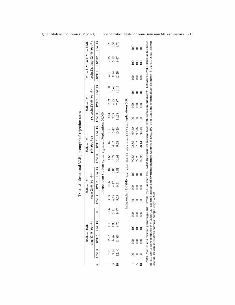
Quantitative Economics 12 (2021) Specification tests for non-Gaussian ML estimators 713
Ta
bl
e3
.St
ruct
ura
lVA
R(1):
emp
iric
alre
ject
ion
rate
s.
%
RM
L=
UM
LU
ML
=P
ML
UM
L=
PM
LU
ML
=P
ML
RM
L=
UM
L&
UM
L=
PM
L
diag(C
)@(θ
T�η
)ve
ch(Σ
)@(θ
T�η
T)
τ@(θ
T�η
T)
(τ�v
ech(Σ))
@(θ
T�η
T)
(vec
h(Σ)�
diag(C
))@(θ
T�η
)
DW
H1
DW
H2
DW
H3
LRD
WH
1D
WH
2D
WH
3D
WH
1D
WH
2D
WH
3D
WH
1D
WH
2D
WH
3D
WH
1D
WH
2D
WH
3
Ind
epen
den
tStu
den
tt(η
1=0�
15�η
2=0�
10),
Rep
licat
ion
s20
,000
12.
702.
221.
111�
063�
392�
063�
041�
651�
161�
513�
642�
093�
314�
612�
763�
285
7�26
6�86
4�98
5�11
6�65
4�17
5�86
5�77
4�87
5�42
7�39
4�85
6�63
8�74
6�18
6�54
1012�4
011�8
89�
769�
979�
756�
518�
8110
�61
9�78
10�2
611�1
87�
8710�1
312
�29
9�47
9�70
Ind
epen
den
tDLS
MN
(δ1�κ
1�λ
1)=(
0�52�0�0
6�0)�(δ
2�κ
2�λ
2)=(
0�3�
0�2�
0�5)
,Rep
licat
ion
s50
00
110
010
010
010
010
010
010
099
�84
92�8
899
�80
100
100
100
100
100
100
510
010
010
010
010
010
010
099
�90
97�0
299
�86
100
100
100
100
100
100
1010
010
010
010
010
010
010
099
�96
98�1
499
�88
100
100
100
100
100
100
Not
e:M
on
teC
arlo
reje
ctio
np
erce
nta
ges.
DW
H1:
Wal
d-t
ype
Hau
sman
test
.DW
H2:
Hau
sman
test
bas
edo
nU
ML
(RM
L)sc
ore
com
pu
ted
atP
MLE
(UM
LE).
DW
H3:
Hau
sman
test
bas
edo
nP
ML
(UM
L)sc
ore
com
pu
ted
atM
LE(R
MLE
).E
xpec
ted
Hes
sian
and
cova
rian
cem
atri
ces
eval
uat
edat
RM
LE(θ
T�η
)o
rP
MLE
and
seq
uen
tial
MM
esti
mat
or(θ
T�η
T).
DLS
MN
(dis
cret
elo
cati
on
-sca
lem
ixtu
reo
ftw
on
orm
als)
.Sam
ple
len
gth
=20
00.

714 Fiorentini and Sentana Quantitative Economics 12 (2021)
Figure 2. Data.
We adopt the original Var(4) specification in Angelini et al. (2019), which impliesthat T = 653 after initialization of the log-likelihood with 4 presample observations. Ourmain point of departure is that we assume that the structural innovations follow threeindependent standardized Student t distributions with νi degrees of freedom, which al-lows us to identify the entire matrix of impact multipliers C = JΨ . Thus, the unrestricted

Quantitative Economics 12 (2021) Specification tests for non-Gaussian ML estimators 715
Table 4. Parameter estimates. Sample period 1960:08–2015:04.
PML UML RML
τ′ 0�013 1�261 0�013 0�008 1�045 −0�007 0�010 1�042 −0�002
J1�000 −0�006 0�069 1�000 −0�008 0�063
14�045 1�000 0�771 21�354 1�000 0�9680�157 −0�001 1�000 0�208 −0�001 1�000
Ψ 0�010 0�681 0�199 0�009 0�582 0�020
JΨ2J′ × 100�001 −0�011 0�001 0�003 0�007 0�027 0�001 −0�009 0�000
−0�011 4�329 0�007 0�007 5�063 0�305 −0�009 3�733 0�0030�001 0�007 0�007 0�027 0�305 0�397 0�000 0�003 0�004
ML procedure estimates 2N + (p+ 1)N2 = 51 parameters, while the restricted MLE fixesν1 = ν2 = ν3 = 8 (We tried different values for the ν’s ranging from 6 to 10 but results werevery similar). Finally, the Gaussian PMLE estimates N(N − 1)/2 = 3 parameters less be-cause it can only identify CC′ = JΨ2J′ =Σ.
Our PML estimators of the autoregressive matrices coincide with those in Angeliniet al. (2019). Further, the restricted and unrestricted MLEs of those parameters are alsovery similar because the three estimators are consistent under weak conditions, as weexplained in Section 3.8. The estimates of the drift, the (scaled) impact multiplier matrixJ, the standard deviations of the structural shocks in Ψ and the unconditional varianceof the one period ahead forecast errors Σ are reported in Table 4. As can be seen, thethree estimators of the drift parameters are quite similar for the first two series, whilefor the last one the sign of the UML and RML estimators is reversed with respect to thePML one. A look at the estimators of Σ reveals both an unbalanced scaling of the data,and a low predictability in the rate of growth of the industrial production index. Therestricted and unrestricted MLEs of J are rather similar. In fact, the consistency of thenon-Gaussian ML estimators of the matrix J is indirectly confirmed by the extremelyhigh (= 0�995) time series correlation between the (nonstandardized) estimates of eachstructural shock obtained as J−1εt(θ) evaluated at the RMLE and UMLE. In contrast,there is a striking difference in the standard deviation of the third structural shock, whichstrongly points to distributional misspecification. However, this conjecture needs to beconfirmed by our formal DWH test statistics, which account for the sampling variabilityof the estimators.
The three versions of our DWH tests produce qualitatively similar results. For thatreason, in Table 5 we only report the results of the versions that evaluate the score of themore efficient estimators at the less efficient ones (e.g., the unrestricted Student t scoresat the Gaussian PMLE). According the Monte Carlo results in the previous section, theseare the most conservative ones. As expected, we conclude that the null of correct spec-ification of the structural innovation distributions is clearly rejected. The test statisticsthat compares the unrestricted ML estimator of the variance of the Wold innovations
JΨ2
J′ with its PML counterpart Σ has a tiny p-value. Similarly, if we compare the sameestimators of the drift parameters, the p-value of our DWH statistic is 0�001. Given the
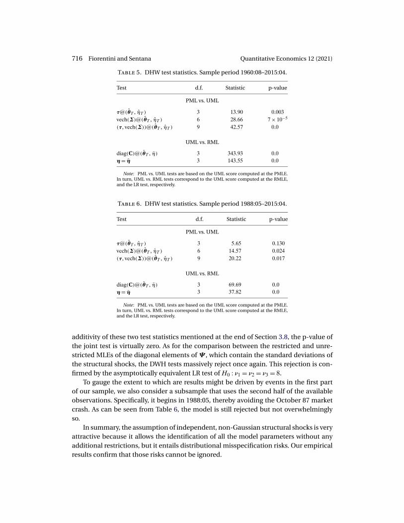
716 Fiorentini and Sentana Quantitative Economics 12 (2021)
Table 5. DHW test statistics. Sample period 1960:08–2015:04.
Test d.f. Statistic p-value
PML vs. UML
τ@(θT � ηT ) 3 13�90 0�003vech(Σ)@(θT � ηT ) 6 28�66 7 × 10⁻⁵
(τ� vech(Σ))@(θT � ηT ) 9 42�57 0�0
UML vs. RML
diag(C)@(θT � η) 3 343�93 0�0η= η 3 143�55 0�0
Note: PML vs. UML tests are based on the UML score computed at the PMLE.In turn, UML vs. RML tests correspond to the UML score computed at the RMLE,and the LR test, respectively.
Table 6. DHW test statistics. Sample period 1988:05–2015:04.
Test d.f. Statistic p-value
PML vs. UML
τ@(θT � ηT ) 3 5�65 0�130vech(Σ)@(θT � ηT ) 6 14�57 0�024(τ� vech(Σ))@(θT � ηT ) 9 20�22 0�017
UML vs. RML
diag(C)@(θT � η) 3 69�69 0�0η= η 3 37�82 0�0
Note: PML vs. UML tests are based on the UML score computed at the PMLE.In turn, UML vs. RML tests correspond to the UML score computed at the RMLE,and the LR test, respectively.
additivity of these two test statistics mentioned at the end of Section 3.8, the p-value ofthe joint test is virtually zero. As for the comparison between the restricted and unre-stricted MLEs of the diagonal elements of Ψ , which contain the standard deviations ofthe structural shocks, the DWH tests massively reject once again. This rejection is con-firmed by the asymptotically equivalent LR test of H0 : ν1 = ν2 = ν3 = 8.
To gauge the extent to which are results might be driven by events in the first partof our sample, we also consider a subsample that uses the second half of the availableobservations. Specifically, it begins in 1988:05, thereby avoiding the October 87 marketcrash. As can be seen from Table 6, the model is still rejected but not overwhelminglyso.
In summary, the assumption of independent, non-Gaussian structural shocks is veryattractive because it allows the identification of all the model parameters without anyadditional restrictions, but it entails distributional misspecification risks. Our empiricalresults confirm that those risks cannot be ignored.

Quantitative Economics 12 (2021) Specification tests for non-Gaussian ML estimators 717
6. Conclusions and directions for further research
We propose an extension of the Durbin–Wu–Hausman specification tests which simul-taneously compares three or more likelihood-based estimators of the parameters of gen-eral multivariate dynamic models with nonzero conditional means and possibly time-varying variances and covariances. Although we focus most of our discussion on thecomparison of the three estimators offered by the dominant commercial econometricpackages, namely, the Gaussian PML estimator, as well as ML estimators based on a non-Gaussian distribution, which either jointly estimate the additional shape parameters orfix them to some plausible values, we also consider two semiparametric estimators, oneof which imposes the assumption that the standardized innovations follow a sphericaldistribution.
We also explore several important issues related to the practical implementationof our proposed tests, including the different versions, their numerical invariance toreparametrizations, and their application to subsets of parameters. By explicitly consid-ering a multivariate framework with nonzero conditional means we are able to covermany empirically relevant applications. Our results also apply to dynamic structuralmodels, whose focus differs from the conditional mean and variance, and raise someinteresting inference issues that we also study in detail. Extensions to stochastic volatil-ity models in which the log-likelihood cannot be obtained in closed form are conceptu-ally possible as long as the ML estimators and their asymptotic variances are available,but we leave the interesting computational considerations that they raise for further re-search.
To select the right number of degrees of freedom, we need to figure out the rank ofthe difference between the estimators’ asymptotic covariance matrices. In this respect,we discuss several situations in which some of the estimators are equally efficient forsome of the parameters and prove that the semiparametric estimators share a saddlepoint efficiency property: they are as inefficient as the Gaussian PMLE for the parame-ters that they cannot estimate adaptively.
A comparison of our results with those in Fiorentini and Sentana (2019) imply thatthe parameters that are efficiently estimated by the semiparametric procedures con-tinue to be consistently estimated by the parametric estimators under distributionalmisspecification. In contrast, the remaining parameters, which the semiparametric pro-cedures can only estimate with the efficiency of the Gaussian PML estimator, will be in-consistently estimated by distributionally misspecified parametric procedures. For thatreason, we focus our tests on the comparison of the estimators of this second group ofparameters, for which the usual efficiency—consistency trade off is of first-order impor-tance.
Our Monte Carlo experiments indicate that many of our proposed tests work quitewell, but some versions show noticeable size distortions in small samples. Since we havea fully specified model under the null, parametric bootstrap versions might be worth ex-ploring. An interesting extension of our Monte Carlo analysis would look at the power ofour tests in models with time-varying shape parameters or misspecified first and secondmoment dynamics.

718 Fiorentini and Sentana Quantitative Economics 12 (2021)
Given the increased popularity of Independent Component Analysis in econometricapplications, as illustrated by the Svars in Section 3.8, specification tests that directlytarget the maintained assumptions of nonnormality and independence of the struc-tural shocks provide a particularly appropriate complement to our proposed tests (seeAmengual, Fiorentini, and Sentana (2021)). We could also extend our theoretical resultsto a broad class of models for which a pseudo log-likelihood function belonging to thelinear exponential family leads to consistent estimators of the conditional mean pa-rameters (see Gouriéroux, Monfort, and Trognon (1984a)). For example, we could usea DWH test to assess the correct distributional specification of Lanne’s (2006) multi-plicative error model for realized volatility by comparing his ML estimator based on atwo-component Gamma mixture with the Gamma-based consistent pseudo ML esti-mators in Engle and Gallo (2006). Similarly, we could also use the same approach to testthe correct specification of the count model for patents in Hausman, Hall, and Griliches(1984) by comparing their ML estimator, which assumes a Poisson model with unob-served gamma heterogeneity, with the consistent pseudo ML estimators in Gouriéroux,Monfort, and Trognon (1984b). All these extensions constitute interesting avenues forfurther research.
Appendix A: Proofs
Proof of Proposition 1. Assuming that θ0 belongs to the interior of its admissibleparameter space, the estimators of θ will be characterized with probability tending to 1by the first-order conditions
∂m′T (θT )
∂θSmT mT (θT ) = 0� (A1)
∂n′T (θT )
∂θSnT nT (θT ) = 0� (A2)
By analogy, θm and θn will be the pseudo-true values of θ implicitly defined by the ex-actly identified moment conditions
J ′m(θm)SmE
[mt (θm)
] = 0�
J ′n(θn)SnE
[nt (θn)
] = 0�
Under the null hypothesis that both sets of moments are correctly specified, we will havethat θm = θn = θ0.
The Wald version of the DWH test in (1) is based on the difference between θT andθT . Under standard regularity conditions (see, e.g., Newey and McFadden (1994)), first-order Taylor expansions of (A1) and (A2) around θ0 imply that
√T(θT − θ0)= −[J ′
m(θ0)SmJm(θ0)]−1J ′
m(θ0)Sm
√TmT (θ0)+ op(1)�
√T(θT − θ0)= −[J ′
n(θ0)Sn(θ0)Jn(θ0)]−1J ′
n(θ0)Sn
√T nT (θ0)+ op(1)�
(A3)

Quantitative Economics 12 (2021) Specification tests for non-Gaussian ML estimators 719
Therefore,
√T(θT − θT ) =
{[J ′m(θ0)SmJm(θ0)
]−1J ′m(θ0)Sm −[J ′
n(θ0)SnJn(θ0)]−1J ′
n(θ0)Sn
}
×[√
TmT (θ0)√T nT (θ0)
]+ op(1)� (A4)
On the other hand, the first score version of the DWH test is as a test of the momentrestrictions
J ′m(θn)SmE
[mt (θn)
]= 0� (A5)
If we knew θn, it would be straightforward to test whether (A5) holds. But since we donot know it, we replace it by its consistent estimator θT , which satisfies (A2). To accountfor the sampling variability that this introduces under the null, we can use again a first-order Taylor expansion around θ0 of the sample version of (A5) evaluated at θT . Giventhe assumed root-T consistency of θT for θ0, we can use (A3) to write this expansion as
J ′m(θT )Sm
√TmT (θT )
= J ′m(θ0)Sm
√TmT (θ0)+J ′
m(θ0)SmJm(θ0)Sm
√T(θT − θ0)+ op(1)
= J ′m(θ0)Sm
√TmT (θ0)
− [J ′m(θ0)SmJm(θ0)
][Jn(θ0)Sn(θ0)J ′
n(θ0)]−1J ′
n(θ0)Sn
√T nT (θ0)+ op(1)� (A6)
But a comparison between (A6) and (A4) makes clear that
√T(θT − θT )= [
J ′m(θ0)SmJm(θ0)
]−1[J ′m(θ0)Sm
√TmT (θT )
]+ op(1)� (A7)
which confirms that the Wald and score versions of the test are asymptotically equiva-lent because rank[J ′
n(θ0)SnJn(θ0)] = dim(θ) in first-order identified models. Given thatmT (θ) and nT (θ) are exchangeable, the second equivalence condition trivially holdstoo.
Proof of Proposition 2. The Wald-type version of the Hausman test for the originalparameters in (1) is infeasible when Δ is unknown, in which case it must be computedas
T(θT − θT )′Δ∼T (θT − θT )� (A8)
where Δ∼T denotes a consistent estimator of a generalized inverse of Δ, which does not
necessarily coincide with a generalized inverse of a consistent estimator of the asymp-totic covariance matrix of
√T(θT − θT ) because of the potential discontinuities of gen-
eralized inverses. Given the assumed regularity of the reparametrization, we can applythe delta method to show that the asymptotic covariance matrix of
√T(πT − πT ) will be
∂θ′(π0)
∂πΔ∂θ(π0)
∂π ′ �

720 Fiorentini and Sentana Quantitative Economics 12 (2021)
which in turn implies that we can use
[∂θ(πT )
∂π ′]−1
Δ∼T
[∂θ′(πT )
∂π
]−1
as a consistent estimator of its generalized inverse provided that πT is a consistent es-timator of π0. Therefore, the Wald-type version of the Hausman test for the original pa-rameters will be
T(πT − πT )′[∂θ(πT )
∂π ′]−1
Δ∼T
[∂θ′(πT )
∂π
]−1(πT − πT )� (A9)
Lemma 1 in Supplemental Appendix B states the numerical invariance of GMM estima-tors and criterion functions to reparametrizations when the weighting matrix remainsthe same, so that
πT − πT = r(θT )− r(θT )�
In general, though, one would expect (A8) and (A9) to differ. However, when the mappingfrom θ to π is affine, the Jacobian of the inverse transformation is the constant matrixA−1, yielding
T(πT − πT )′A′−1Δ∼
T A−1(πT − πT ) = T(θT − θT )′Δ∼T (θT − θT )�
as required.Let us now look at one of the score versions of the DWH test in terms of the original
parameters, the other one being entirely analogous. We saw in the proof of the previousproposition that the first-order condition for θT is (A1). Therefore, we can compute thealternative DWH test in practice as
Tm′T (θT )SmT
∂mT (θT )
∂θ′ Λ∼mT
∂m′T (θT )
∂θSmT mT (θT )� (A10)
Lemma 1 also implies that mT (π) = mT [θ(π)] and θT = θ(πT ) when the weight-ing matrix used to compute θT and πT is common. Given the assumed regularity ofthe reparametrization, we can easily show that the asymptotic covariance matrix ofJ ′m(π0)Sm
√T mT (πT ) will be
Λm = ∂θ′(π0)
∂πΛm
∂θ(π0)
∂π ′ �
As a consequence, it seems natural to use
[∂θ(πT )
∂π ′]−1
Λ∼mT
[∂θ′(πT )
∂π
]−1(A11)
as a consistent estimator of a generalized inverse ofΛm, provided that πT is a consistentestimator of π0. Therefore, we can compute the analogous test in terms of π as
T m′T (πT )SmT
∂mT (πT )
∂π ′[∂θ(πT )
∂π ′]−1
Λ∼mT
[∂θ′(πT )
∂π
]−1 ∂m′T (πT )
∂πSmT mT (πT )� (A12)

Quantitative Economics 12 (2021) Specification tests for non-Gaussian ML estimators 721
Combining the chain rule for derivatives with the results in Lemma 1, we can prove
that
∂m′T (πT )
∂πSmT mT (πT )= ∂θ′(πT )
∂π
∂m′T (θT )
∂θSmT mT (θT )�
which in turn implies that
m′T (πT )SmT
∂mT (πT )
∂π ′[∂θ(πT )
∂π ′]−1
Λ∼mT
[∂θ′(πT )
∂π
]−1 ∂m′T (πT )
∂πSmT mT (πT )
= m′T (θT )SmT
∂mT (θT )
∂θ′∂θ(πT )
∂π ′[∂θ(πT )
∂π ′]−1
Λ∼mT
[∂θ′(πT )
∂π
]−1
× ∂θ′(πT )
∂π
∂m′T (θT )
∂θSmT mT (θT )�
Therefore, (A10) and (A12) will be numerically identical if
∂θ(πT )
∂π ′[∂θ(πT )
∂π ′]−1
= Ip�
Sufficient conditions for this to happen are that the mapping is affine, or that we use
πT = πT in computing (A11).
Proof of Proposition 3. Again, we focus on the first result, as the second one is en-
tirely analogous. Let us start from the asymptotic equivalence relationship (A7). Given
that
J ′m(θ0)SmJm(θ0) =
[J ′
1m(θ)SmJ1m(θ) J ′1m(θ)SmJ2m(θ)
J ′2m(θ)SmJ1m(θ) J ′
2m(θ)SmJ2m(θ)
]and
J ′m(θ0)Sm
√TmT (θT ) =
[J ′
1m(θ)Sm
√TmT (θT )
J ′2m(θ)Sm
√TmT (θT )
]�
the application of the partitioned inverse formula yields
√T(θ1T − θ1T ) = [
J ′m(θ0)SmJm(θ0)
]11m⊥1T (θT �Sm)� where
[J ′m(θ0)SmJm(θ0)
]11 =[
J ′1m(θ)SmJ1m(θ)
−J ′1m(θ)SmJ2m(θ)
[J ′
2m(θ)SmJ2m(θ)]−1J ′
2m(θ)SmJ1m(θ)
]−1
�
Given that [J ′m(θ0)SmJm(θ0)]11 will have rank p1 because [J ′
m(θ0)SmJm(θ0)] has
rank p, the Wald version of the DWH test that focuses on θ1 only is equivalent to a score
version that looks at m⊥1T (θT �Sn).

722 Fiorentini and Sentana Quantitative Economics 12 (2021)
Proof of Proposition 4. Given that
⎛⎜⎜⎜⎜⎜⎜⎜⎜⎝
θ2T − θ1
T
θ3T − θ2
T���
θJ−1T − θJ−2
T
θJT − θJ−1
T
⎞⎟⎟⎟⎟⎟⎟⎟⎟⎠
=
⎡⎢⎢⎢⎢⎢⎢⎣
−I I 0 � � � 0 0 00 −I I � � � 0 0 0���
���� � �
� � ����
������
0 0 0 � � � −I I 00 0 0 � � � 0 −I I
⎤⎥⎥⎥⎥⎥⎥⎦
⎛⎜⎜⎜⎜⎜⎜⎜⎜⎜⎜⎜⎜⎜⎝
θ1T
θ2T
θ3T���
θJ−2T
θJ−1T
θJT
⎞⎟⎟⎟⎟⎟⎟⎟⎟⎟⎟⎟⎟⎟⎠� (A13)
it follows immediately from (5) that
limT→∞
V
⎡⎢⎢⎢⎢⎢⎢⎢⎢⎣
√T
⎛⎜⎜⎜⎜⎜⎜⎜⎜⎝
θ2T − θ1
T
θ3T − θ2
T���
θJ−1T − θJ−2
T
θJT − θJ−1
T
⎞⎟⎟⎟⎟⎟⎟⎟⎟⎠
⎤⎥⎥⎥⎥⎥⎥⎥⎥⎦
=
⎡⎢⎢⎢⎢⎢⎢⎣
Ω2 −Ω1 0 � � � 0 00 Ω3 −Ω2 � � � 0 0���
���� � �
������
0 0 � � � ΩJ−1 −ΩJ−2 00 0 � � � 0 ΩJ −ΩJ−1
⎤⎥⎥⎥⎥⎥⎥⎦� (A14)
which in turn implies the asymptotic independence of nonoverlapping DWH test statis-tics of the form (1). But since (A13) holds for any T , all J(J − 1)/2 possible differencesbetween any two of the J estimators will be linear combinations of the J − 1 adjacentdifferences in (A14).
Proof of Proposition 5. Given that Propositions C1–C3 in Supplemental Appendix Cand Proposition D3 in Supplemental Appendix D derive all the information bounds,we simply need to compute the off-diagonal elements. Let us start with the first row.Straightforward manipulations imply that
E[sθt (φ)s′
θ|ηt (φ)|φ] = E
{sθt (φ)
[s′θt (φ)− s′
ηt (φ)I−1ηη(φ)I ′
θη(φ)]|φ}
= Iθθ(φ)− Iθη(φ)I−1ηη(φ)I ′
θη(φ)= P(φ)�
Intuitively, P(φ0) is the covariance matrix of the residuals in the multivariate theoreticalregression of sθt (φ0) on sηt (φ0), which trivially coincides with the covariance matrixbetween those residuals and sθt (φ0). Next,
E[sθt (φ)s′
θt (φ)|φ]
=E[Zdt(θ)edt(φ)
{e′dt(φ)Z′
dt(θ)− [e′dt(φ)− e′
dt(θ�0)K+(κ)K(0)]Z′d(φ)
}|φ]

Quantitative Economics 12 (2021) Specification tests for non-Gaussian ML estimators 723
=E[Zdt(θ)edt(φ)e′
dt(φ)Zdt(θ)|φ]
−E{
Zdt(θ)edt(φ)[e′dt(φ)− e′
dt(θ�0)K+(κ)K(0)]Z′d(φ)|φ
}= Iθθ(φ0)− Ws(φ0)W′
s(φ0) ·{[
N + 2N
mss(η0)− 1]
− 4N[(N + 2)κ0 + 2
]}= S(φ0)
by virtue of the law of iterated expectations, together with expressions (C33), (C34),and (C35) in Supplemental Appendix C. Intuitively, S(φ0) is the variance of the errorin the least squares projection of sθt (φ0) onto the Hilbert space spanned by all the time-invariant functions of ς t (θ0) with bounded second moments that have zero conditionalmeans and are conditionally orthogonal to edt(θ0�0), which trivially coincides with thecovariance matrix between those residuals and sθt (φ0). Given that this Hilbert space in-cludes the linear span of sηt (φ0), it follows immediately that S(φ0) is smaller than P(φ0)
in the positive semidefinite sense.We also know from the proof of Proposition D3 in Supplemental Appendix D that
E[sθt (φ)s′
θt (φ)|φ]
=E[Zdt(θ)edt(φ)
{e′dt(φ)Z′
dt(θ)− [e′dt(φ)− e′
dt(θ�0)K+(�)K(0)]Z′d(φ)
}|φ]=E
[Zdt(θ)edt(θ��)e′
dt(θ��)Zdt(θ)|φ]
−E{
Zdt(θ)edt(φ)[e′dt(φ)− e′
dt(θ�0)K+(�)K(0)]Z′d(φ)|φ
}= Iθθ(φ)− Zd(φ)
[Mdd(�0)−K(0)K+(�0)K(0)
]Z′d(φ) = S(φ0)
by virtue of the law of iterated expectations, together with expressions (B3) and (C22) inSupplemental Appendices B and C, respectively. Intuitively, S(φ0) is the covariance ma-trix of the errors in the projection of sθt (φ0) onto the Hilbert space spanned by all thetime-invariant functions of ε∗
t with zero conditional means and bounded second mo-ments that are conditionally orthogonal to edt(θ0�0), which trivially coincides with thecovariance matrix between those residuals and sθt (φ0). The fact that the residual vari-ance of a multivariate regression cannot increase as we increase the number of regres-sors explains why S(φ0) is at least as large (in the positive semidefinite matrix sense) asS(φ0), reflecting the fact that the relevant tangent sets become increasing larger. Finally,
E[sθt (φ)s′
θt (θ�0)|φ]= −∂E[s′θt (θ�0)|φ]/∂θ= A(φ)
thanks to the generalized information equality.Let us now move on to the second row, and in particular to
E[sθ|ηt (φ)s′
θt (φ)|φ]
= E[{
Zdt(θ)edt(φ)− Iθη(φ)I−1ηη(φ)ert(φ)
}× {
e′dt(φ)Z′
dt(θ)− [e′dt(φ)− e′
dt(θ�0)K+(κ)K(0)]Z′d(φ)
}|φ]= E
[{Zdt(θ)edt(φ)e′dt(φ0)Z′
dt(φ0)|φ]−E
[Zdt(θ)edt(φ)e′
dt(φ)Z′dt(φ0)|φ
]+E
[Zdt(θ)edt(φ)e′
dt(θ�0)K+(�0)K(0)Z′d(φ)|φ
]

724 Fiorentini and Sentana Quantitative Economics 12 (2021)
− Iθη(φ)I−1ηη(φ)E
[ert(φ)e′
dt(φ)Z′dt(θ)|φ
]+ Iθη(φ)I−1
ηη(φ)E[ert(φ)e′
dt(φ)Z′d(θ)|φ
]− Iθη(φ)I−1
ηη(φ)E[ert(φ)e′
dt(θ�0)K+(κ)K(0)Z′d(φ)|φ
]= Iθθ(φ)− Ws(φ0)W′
s(φ0) ·{[
N + 2N
mss(η0)− 1]
− 4N[(N + 2)κ0 + 2
]}= S(φ0)
where we have used the fact that
E[ert(φ)e′
dt(φ)|φ] = E
{E[ert(φ)e′
dt(φ)|ςt�φ]|φ}=E
[ert(φ)e′
dt(φ)|φ]
= E{
ert(φ)[δ(ςt�η)(ςt/N)− 1
]|φ}[0 vec′(IN)]
and
E[ert(φ)e′
dt(θ�0)|φ] = E{E[ert(φ)e′
dt(θ�0)|ςt�φ]|φ}= E
[ert(φ)e′
dt(θ�0)|φ]= E
{ert(φ)
[(ςt/N)− 1
]|φ}[0 vec′(IN)]= 0
by virtue of Lemma 3 in Supplemental Appendix B. Similarly,
E[sθ|ηt (φ)s′
θt (φ)|φ]
= E[{
Zdt(θ)edt(φ)− Iθη(φ)I−1ηη(φ)ert(φ)
}× {
e′dt(φ0)
[Z′dt(φ0)− Z′
d(φ)]− e′
dt(θ0�0)K+(�0)K(0)Z′d(φ)
}|φ]= E
[Zdt(θ)edt(φ)e′
dt(φ0)Z′dt(φ0)|φ
]−E[Zdt(θ)edt(φ)e′
dt(φ0)Z′d(φ)|φ]
−E[Zdt(θ)edt(φ)e′
dt(θ�0)K+(�0)K(0)Z′d(θ)|φ
]= Iθθ(φ)− Zd(φ)
[Mdd(�0)−K(0)K+(�0)K(0)
]Z′d(φ) = S(φ0)
because sηt (φ) is orthogonal to edt(θ�0) by virtue of Lemma 3 and
E[ert(φ)}
{e′dt(φ0)
[Z′dt(φ0)− Z′
d(φ)]}|φ]= 0
by the law of iterated expectations. Finally,
E[sθ|ηt (φ)s′
θt (θ�0)|φ]=E[{
Zdt(θ)edt(φ)− Iθη(φ)I−1ηη(φ)ert(φ)
}e′dt(θ�0)Z′
dt(φ)|φ]
= A(φ)
because of the generalized information equality and the orthogonality of ert(φ) andedt(θ�0).
Let us start the third row with
E[sθt (φ)s′
θt (φ)|φ]= E
[{Zdt(θ)edt(φ)− Zd(φ)
[edt(φ)− K(0)K+(κ)edt(θ�0)
]}× {
e′dt(φ0)
[Z′dt(φ0)− Z′
d(φ)]− e′
dt(θ0�0)K+(�0)K(0)Z′d(φ)
}|φ]= Iθθ(φ)− Zd(φ)
[Mdd(�0)−K(0)K+(�0)K(0)
]Z′d(φ) = S(φ0)

Quantitative Economics 12 (2021) Specification tests for non-Gaussian ML estimators 725
because
E{[
edt(φ)− K(0)K+(κ)edt(θ�0)]e′dt(φ0)
[Z′dt(φ0)− Z′
d(φ)]|φ}= 0
by the law of iterated expectations. In addition, we have that
E[sθt (φ)s′
θt (θ�0)|φ]= A(φ)� (A15)
which follows immediately from (A21) and the generalized information matrix equality.Turning to the last off-diagonal element, we can show that
E[sθt (φ)s′
θt (θ�0)|φ]=E[{
Zdt(θ)edt(θ��)− Zd(θ��)[edt(θ��)−K(0)K+(�)edt(θ�0)
]}× e′
dt(θ�0)Z′dt(θ)|φ
]=A(θ)
because edt(θ�0) is conditionally orthogonal to [edt(θ��)−K(0)K+(�)edt(θ�0)] by con-struction. This result also proves the positive semidefiniteness of S(φ0)−A(θ)B−1(φ)×A(θ) because this expression coincides with the residual covariance matrix in the theo-retical regression of the semiparametric efficient score on the Gaussian pseudo-score.
To prove the second part of the proposition, it is convenient to regard each estima-tor as an exactly identified GMM estimator based on the corresponding score, whoseasymptotic variance depends on the asymptotic variance of this score and the corre-sponding expected Jacobian. In this regard, note that the information matrix equalityapplied to the restricted and unrestricted versions of the efficient score implies that
−∂E[sθt (φ)|φ
]/∂θ′ = E
[sθt (φ)s′
θt (φ)|φ]= Iθθ(φ) and
−∂E[sθ|ηt (φ)|φ
]/∂θ′ = E
[sθ|ηt (φ)s′
θ|ηt (φ)|φ]= P(φ)�
Similarly, we can use the generalized information matrix equality together with someof the arguments in the proof of Proposition C3 in Supplemental Appendix C to showthat
− ∂E[sθt (φ)|φ
]/∂θ
= E[sθt(φ0)s′
θt (φ0)|φ]
= E[Zdt(θ0)edt(φ0)e′
dt(φ0)Z′dt(θ0)
∣∣∣φ0]
−E
{Ws(φ0)
[[δ(ςt�η0)
ςt
N− 1
]
− 2(N + 2)κ0 + 2
(ςt
N− 1
)]e′dt(φ0)Z′
dt(θ0)∣∣∣φ0
}
= Iθθ(φ0)− Ws(φ0)E
{[{δ(ςt�η0)
ςt
N− 1
}
− 2(N + 2)κ0 + 2
(ςt
N− 1
)]e′dt(φ0)
∣∣∣φ0
}Zd(θ0)

726 Fiorentini and Sentana Quantitative Economics 12 (2021)
= Iθθ(φ0)− Ws(φ0)E
[{[δ(ςt�η0)
ςt
N− 1
]
− 2(N + 2)κ0 + 2
(ςt
N− 1
)}[δ(ςt�η0)
ςt
N− 1
]∣∣∣φ0
]W′
s(φ0)
= Iθθ(φ0)− Ws(φ0)W′s(φ0) ·
{[N + 2N
mss(η0)− 1]
− 4N[(N + 2)κ0 + 2
]}
= S(φ0)= E[sθt (φ)s′
θt (φ)|φ]� (A16)
The generalized information matrix equality also implies that
−∂E[sθt (φ0)|φ0
]∂θ
=E[sθt (φ0)s′
θt (φ0)|φ]=E
[Zdt(θ0)edt(φ0)e′
dt(φ0)Z′dt(θ0)|φ0
]�
On this basis, we can use standard first-order expansions of√T [θT (η0) − θ0] and√
T(θT − θ0) to show that
limT→∞
E{T[θT (η0)− θ0
](θ
′T − θ′
0)}= I−1
θθ (φ) limT→∞
E[T sθT (φ)s′θ|ηT (φ)}P−1(φ) = I−1
θθ (φ)�
All the remaining asymptotic covariances are obtained analogously.
Proof of Proposition 6. Given the efficiency of θT relative to θT , it follows fromLemma 2 in Hausman (1978) that
√T(θT − θT ) →N
[0�C(φ0)−P−1(φ0)
]�
The other two results follow directly from Proposition 1 after taking into account that
−∂E[sθ|ηt (φ)|φ
]/∂θ′ = P(φ)�
−∂E[sθt (θ�0)|φ]/∂θ′ = A(φ)
(A17)
by the generalized information matrix equality.
Proof of Proposition 7. The efficiency of θT (η) relative to θT and Lemma 2 in Haus-man (1978) imply that
√T[θT − θT (η)
]→ N[0�Iθθ(φ0)− I−1
θθ (φ0)]
under then null of correct specification. The other two results follow directly fromProposition 1 and the partitioned inverse formula after taking into account (A17) and
−∂E[sθt (θ� η)|φ
]/∂θ′ = Iθθ(φ)
by the information matrix equality.
Proof of Proposition 8. The proof of Proposition 6 immediately implies that√T(θT − θT ) →N
[0�Cθ1θ1(φ0)−Pθ1θ1(φ0)
]

Quantitative Economics 12 (2021) Specification tests for non-Gaussian ML estimators 727
under the null. If we combine this result with Proposition 3, we obtain the expressionsfor the asymptotic variances of the two asymptotically equivalent score versions.
Proof of Proposition 9. The proof of Proposition 7 immediately implies that
√T[θ1T − θ1T (η)
]→N{
0�[Pθ1θ1(φ0)− Iθ1θ1(φ0)
]}under the null. If we combine this result with Proposition 3, we obtain the expressionsfor the asymptotic variances of the two asymptotically equivalent score versions.
Proof of Proposition 10. The proof of the first part is trivial, except perhaps for thefact that Msr(0) = 0, which follows from Lemma 3 in Supplemental Appendix B becauseest(θ0�0) coincides with est(θ0��0) under normality.
To prove the second part, we use the fact that after some tedious algebraic manipu-lations we can write Mdd(η)−K(0)K+(κ)K(0) in the spherical case as
⎧⎨⎩[mll(η)− 1
]IN 0
0[
mss(η)− 1κ+ 1
](IN2 + KNN)+
[mss(η0)− 1 + 2κ
(κ+ 1)[(N + 2)κ+ 2
] ] vec(IN) vec′(IN)
⎫⎬⎭ �
Therefore, given that Zl(φ0) �= 0, Iθθ(φ) − S(φ) will be zero only if mll(η) = 1, which inturn requires that the residual variance in the multivariate regression of δ(ςt�η0)ε
∗t on ε∗
t
is zero for all t, or equivalently, that δ(ςt�η0) = 1. But since the solution to this differen-tial equation is g(ςt�η) = −�5ςt + C, then the result follows from (C19) in SupplementalAppendix C.
If the true conditional mean were 0, and this was taken into account in estimation,then the first diagonal block would disappear, and Iθθ(φ)− S(φ) could also be 0 if
Zd(θ��)[Mdd(�)−K(0)K+(�)K(0)
]Z′d(θ��) = 0�
Although this condition is unlikely to hold otherwise, it does not strictly speaking requirenormality. For example, Amengual, Fiorentini, and Sentana (2013), correcting an earliertypo in Amengual and Sentana (2010), showed that
mss(η0) = Nκ+ 2(N + 2)κ+ 2
for the Kotz distribution, which immediately implies that
mss(η)− 1κ+ 1
= Nκ2
(κ+ 1)(2κ+Nκ+ 2)and
mss(η0)− 1 + 2κ(κ+ 1)
[(N + 2)κ+ 2
] = − 2κ2
(κ+ 1)(2κ+Nκ+ 2)�
When N = 1, (IN2 + KNN) = 2 and vec(IN) vec′(IN) = 1, which trivially implies thatIθθ(φ) − S(φ) = 0. However, this result fails to hold for N ≥ 2. Specifically, using the

728 Fiorentini and Sentana Quantitative Economics 12 (2021)
explicit expressions for the commutation matrix in Magnus (1988), it is straightforwardto show that
κ2
(κ+ 1)(4κ+ 2)
⎛⎜⎜⎜⎝
2 0 0 00 1 1 00 1 1 00 0 0 2
⎞⎟⎟⎟⎠− κ2
(κ+ 1)(2κ+ 1)
⎛⎜⎜⎜⎝
1001
⎞⎟⎟⎟⎠(
1 0 0 1)
=
⎛⎜⎜⎜⎜⎜⎜⎜⎜⎜⎜⎜⎝
κ2
(κ+ 1)(2κ+ 1)0 0 − κ2
(κ+ 1)(2κ+ 1)
0κ2
(κ+ 1)(2κ+ 1)κ2
(κ+ 1)(2κ+ 1)0
0κ2
(κ+ 1)(2κ+ 1)κ2
(κ+ 1)(2κ+ 1)0
− κ2
(κ+ 1)(2κ+ 1)0 0
κ2
(κ+ 1)(2κ+ 1)
⎞⎟⎟⎟⎟⎟⎟⎟⎟⎟⎟⎟⎠�
which can only be 0 under normality.
Proof of Proposition 11. Note that Iθθ(φ)− S(φ) is Ws(φ)W′s(φ) times the residual
variance in the theoretical regression of δ(ςt�η0)ςt/N − 1 on (ςt/N)− 1. Therefore, giventhat Ws(φ) �= 0, Iθθ(φ)− S(φ) can only be 0 if that regression residual is identically 0 forall t. The solution to the resulting differential equation is
g(ςt�η)= − N(N + 2)κ2[(N + 2)κ+ 2
] ln ςt − 1[(N + 2)κ+ 2
]ςt +C�
which in view of (C19) in Supplemental Appendix C implies that
h(ςt;η)∝ ςN
(N+2)κ+2 −1t exp
{− 1[
(N + 2)κ+ 2]ςt}�
i.e., the density of Gamma random variable with mean N and variance N[(N +2)κ0 +2].In this sense, it is worth recalling that κ≥ −2/(N + 2) for all spherical distributions, withthe lower limit corresponding to the uniform.
As for the second part, expression (C27) in Supplemental Appendix C implies that inthe spherically symmetric case the difference between P(φ0) and Iθθ(φ0) is given by
Ws(φ0)W′s(φ0) · [msr(η0)M−1
rr (η0) m′sr(η0)
]�
which is the product of a rank one matrix times a nonnegative scalar. Therefore, giventhat Ws(φ) �= 0 and Mrr(η0) has full rank, P(φ0) can only coincide with Iθθ(φ0) if the1 × q vector msr(η0) is identically 0.
Proof of Proposition 12. Given our assumptions on the mapping rs(·), we can di-rectly work in terms of the ϑ parameters. In this sense, since the conditional covariance

Quantitative Economics 12 (2021) Specification tests for non-Gaussian ML estimators 729
matrix of yt is of the form ϑiΣ◦t (ϑc), it is straightforward to show that
Zdt(ϑ) ={ϑ
−1/2i
[∂μ′
t (ϑc)/∂ϑc]Σ
◦−1/2′t (ϑc)
0
12{∂ vec′[Σ◦
t (ϑc)]/∂ϑc
}[Σ
◦−1/2′t (ϑc)⊗Σ◦−1/2′
t (ϑc)]
12ϑ−1i vec′(IN)
⎫⎪⎬⎪⎭
=[
Zϑclt(ϑ) Zϑcst(ϑ)
0 Zϑist(ϑ)
]� (A18)
Thus, the score vector for ϑ will be[sϑct(ϑ�η)
sϑit(ϑ�η)
]=[
Zϑclt(ϑ)elt (ϑ�η)+ Zϑcst(ϑ)est(ϑ�η)Zϑist(ϑ)est(ϑ�η)
]� (A19)
where elt (ϑ�η) and est(ϑ�η) are given in expressions (C8) and (C9) in SupplementalAppendix C, respectively.
It is then easy to see that the unconditional covariance between sϑct(ϑ�η) andsϑit(ϑ�η) is
E
{[Zϑclt(ϑ) Zϑcst(ϑ)
][Mll(η) 00 Mss(η)
][0
Z′ϑist
(ϑ)
]∣∣∣ϑ�η}
={2mss(η)+N
[mss(η)− 1
]}2ϑi
×E
{12∂ vec′[Σ◦
t (ϑc)]
∂ϑc
[Σ
◦−1/2′t (ϑc)⊗Σ◦−1/2′
t (ϑc)]∣∣∣ϑ�η} vec(IN)
={2mss(η)+N
[mss(η)− 1
]}2ϑi
Zϑcs(ϑ�η) vec(IN)�
with Zϑcs(ϑ�η)= E[Zϑcst(ϑ)|ϑ�η], where we have exploited the serial independence ofε∗t , as well as the law of iterated expectations, together with the results in Proposition C1
in Supplemental Appendix C.We can use the same arguments to show that the unconditional variance of sϑit(ϑ�η)
will be given by
E
{[0 Zϑist(ϑ)
][Mll(η) 00 Mss(η)
][0
Z′ϑist
(ϑ)
]∣∣∣ϑ�η}
= 1
4ϑ2i
vec′(IN)[mss(η)(IN2 + KNN)+ [
mss(η)− 1]) vec(IN) vec′(IN)
]vec(IN)
={2mss(η)+N
[mss(η)− 1
]}N
4ϑ2i
�
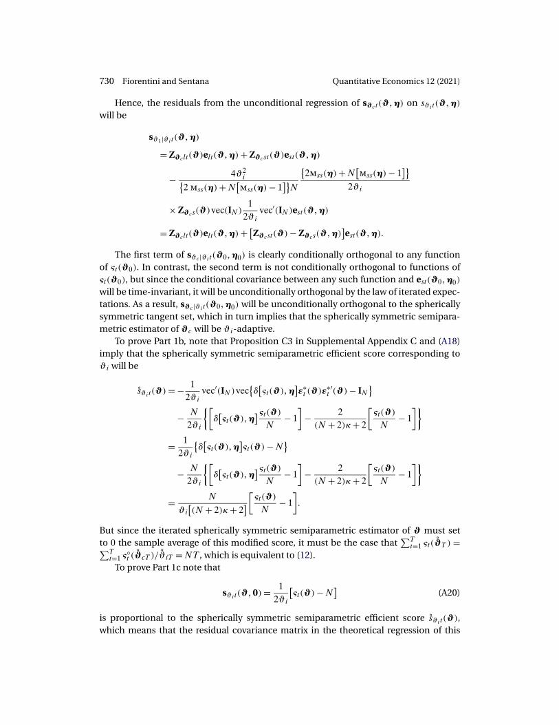
730 Fiorentini and Sentana Quantitative Economics 12 (2021)
Hence, the residuals from the unconditional regression of sϑct(ϑ�η) on sϑit(ϑ�η)
will be
sϑ1|ϑit(ϑ�η)
= Zϑclt(ϑ)elt (ϑ�η)+ Zϑcst(ϑ)est(ϑ�η)
− 4ϑ2i{
2 mss(η)+N[mss(η)− 1
]}N
{2mss(η)+N
[mss(η)− 1
]}2ϑi
× Zϑcs(ϑ) vec(IN)1
2ϑivec′(IN)est(ϑ�η)
= Zϑclt(ϑ)elt (ϑ�η)+ [Zϑcst(ϑ)− Zϑcs(ϑ�η)
]est(ϑ�η)�
The first term of sϑc |ϑit(ϑ0�η0) is clearly conditionally orthogonal to any functionof ςt(ϑ0). In contrast, the second term is not conditionally orthogonal to functions ofςt(ϑ0), but since the conditional covariance between any such function and est(ϑ0�η0)
will be time-invariant, it will be unconditionally orthogonal by the law of iterated expec-tations. As a result, sϑc |ϑit(ϑ0�η0) will be unconditionally orthogonal to the sphericallysymmetric tangent set, which in turn implies that the spherically symmetric semipara-metric estimator of ϑc will be ϑi-adaptive.
To prove Part 1b, note that Proposition C3 in Supplemental Appendix C and (A18)imply that the spherically symmetric semiparametric efficient score corresponding toϑi will be
sϑit(ϑ) = − 12ϑi
vec′(IN) vec{δ[ςt(ϑ)�η
]ε∗t (ϑ)ε
∗′t (ϑ)− IN
}
− N
2ϑi
{[δ[ςt(ϑ)�η
]ςt(ϑ)N
− 1]
− 2(N + 2)κ+ 2
[ςt(ϑ)
N− 1
]}
= 12ϑi
{δ[ςt(ϑ)�η
]ςt(ϑ)−N
}
− N
2ϑi
{[δ[ςt(ϑ)�η
]ςt(ϑ)N
− 1]
− 2(N + 2)κ+ 2
[ςt(ϑ)
N− 1
]}
= N
ϑi
[(N + 2)κ+ 2
][ςt(ϑ)N
− 1]�
But since the iterated spherically symmetric semiparametric estimator of ϑ must setto 0 the sample average of this modified score, it must be the case that
∑Tt=1 ςt(ϑT ) =∑T
t=1 ς◦t (ϑcT )/ϑiT =NT , which is equivalent to (12).
To prove Part 1c note that
sϑit(ϑ�0) = 12ϑi
[ςt(ϑ)−N
](A20)
is proportional to the spherically symmetric semiparametric efficient score sϑit(ϑ),which means that the residual covariance matrix in the theoretical regression of this

Quantitative Economics 12 (2021) Specification tests for non-Gaussian ML estimators 731
efficient score on the Gaussian score will have rank p − 1 at most. But this residual co-variance matrix coincides with S(φ)−A(φ)B−1(φ)A(φ) since
E[sθt (φ)s′
θt (θ�0)|φ]=E[Zdt(θ)edt(φ)e′
dt(θ�0)Z′dt(θ)|φ
]= A(θ) (A21)
because the regression residual[δ(ςt�η)
ςt
N− 1
]− 2
(N + 2)κ0 + 2
(ςt
N− 1
)
is conditionally orthogonal to edt(θ0�0) by the law of iterated expectations, as shown inthe proof of Proposition C3 in Supplemental Appendix C.
Tedious algebraic manipulations that exploit the block-triangularity of (A18) andthe constancy of Zϑist(ϑ) show that the different information matrices will be blockdiagonal when Wϑcs(φ0) is 0. Then, Part 2a follows from the fact that Wϑcs(φ0) =−E{∂dt(ϑ0)/∂ϑc|φ0} will trivially be 0 if E[ln |Σ◦
t (ϑc)||φ0] = k ∀ϑc .Finally, to prove Part 2b note that (A20) implies that the Gaussian PMLE will also
satisfy (12). But since the asymptotic covariance matrices in both cases will be block-diagonal between ϑc and ϑi when E[ln |Σ◦
t (ϑc)||φ0] = k ∀ϑc , the effect of estimating ϑc
becomes irrelevant.
Proof of Proposition 13. We can directly work in terms of the ϕ parameters thanksto our assumptions on the mapping rg(·). Given the specification for the conditionalmean and variance in (14), and the fact that ε∗
t is assumed to be i�i�d� conditional on ztand It−1, it is tedious but otherwise straightforward to show that the score vector will be⎡
⎢⎣ sϕ1t (ϕ��)
sϕic t (ϕ��)
sϕimt(ϕ��)
⎤⎥⎦=
⎡⎢⎣Zϕ1lt (ϕ)elt (ϕ��)+ Zϕ1st(ϕ)est(ϕ��)
Zϕicst (ϕ)est(ϕ��)Zϕimlt(ϕ)elt (ϕ��)
⎤⎥⎦ � (A22)
where
Zϕ1lt (ϕ) = {∂μ�′
t (ϕ1)/∂ϕ1 + ∂ vec′[Σ�1/2t (ϕ1)
]/∂ϕ1 · (ϕim ⊗ IN)
}Σ
�−1/2′t (ϕ1)Φ
−1/2′2 �
Zϕ1st(ϕ) = ∂ vec′[Σ�1/2t (ϕ1)
]/∂ϕ1 · [Φ1/2
2 ⊗Σ�−1/2′t (ϕ1)Φ
−1/2′2
]�
Zϕimlt(ϕ) =Φ−1/2′2 = Zϕiml(ϕ)�
Zϕicst(ϕ)= ∂ vec′(Φ1/2)/∂ϕic · (IN ⊗Φ−1/2′2
)= Zϕics(ϕ)�
⎫⎪⎪⎪⎪⎪⎪⎪⎬⎪⎪⎪⎪⎪⎪⎪⎭
(A23)
elt(ϕ��) and est(ϕ��) are given in (D4) in Supplemental Appendix D, with
ε∗t (ϕ) =Φ−1/2
ic Σ�−1/2t (ϕc)
[yt −μ�
t (ϕc)−Σ�1/2t (ϕc)ϕim
]� (A24)
It is then easy to see that the unconditional covariance between sϕct(ϕ��) and theremaining elements of the score will be given by
[Zϕcl(ϕ��) Zϕcs(ϕ��)
][Mll(�) Mls(�)
M′ls(�) Mss(�)
][0 Z′
ϕiml(ϕ)
Z′ϕics
(ϕ) 0
]

732 Fiorentini and Sentana Quantitative Economics 12 (2021)
with Zϕcl(ϕ��) = E[Zϕclt(ϕ)|ϕ��] and Zϕcs(ϕ��) = E[Zϕcst(ϕ)|ϕ��], where we have ex-ploited the serial independence of ε∗
t and the constancy of Zϕicst (ϕ) and Zϕimlt(ϕ), to-gether with the law of iterated expectations and the definition[
Mll(�) Mls(�)
M′ls(�) Mss(�)
]= V
[elt(ϕ��)est(ϕ��)
∣∣∣ϕ��]�
Similarly, the unconditional covariance matrix of sϕic t (ϕ��) and sϕimt(ϕ��) will be
[0 Zϕics(ϕ)
Zϕiml(ϕ) 0
][Mll(�) Mls(�)
M′ls(�) Mss(�)
][0 Z′
ϕiml(ϕ)
Z′ϕics
(ϕ) 0
]�
Thus, the residuals from the unconditional least squares projection of sϕct(ϕ��) onsϕic t (ϕ��) and sϕimt(ϕ��) will be
sϕc |ϕic �ϕimt(ϕ��) = Zϕclt(ϕ)elt (ϕ��)+ Zϕcst(ϕ)est(ϕ��)
−[
Zϕcl(ϕ��) Zϕcs(ϕ��)][elt(ϕ��)
est(ϕ��)
]
= [Zϕclt(ϕ)− Zϕcl(ϕ��)
]elt (ϕ��)+ [
Zϕcst(ϕ)− Zϕcs(ϕ��)]est(ϕ��)�
because both Zϕics(ϕ) and Zϕiml(ϕ) have full row rank when Φic has full rank in view ofthe discussion that follows expression (D13) in Supplemental Appendix D.
Neither elt (ϕ��) nor est(ϕ��) will be conditionally orthogonal to arbitrary functionsof ε∗
t . But their conditional covariance with any such function will be time-invariant.Hence, sϕc |ϕic �ϕimt(ϕ��) will be unconditionally orthogonal to ∂ ln f [ε∗
t (ϕ);�]/∂� byvirtue of the law of iterated expectations, which in turn implies that the unrestrictedsemiparametric estimator of ϕc will be ϕi-adaptive.
To prove Part 1b, note that the semiparametric efficient scores corresponding to ϕic
and ϕim will be given by[0 Zϕics(ϕ)
Zϕiml(ϕ) 0
]K(0)K+(�0)
{ε∗t (ϕ)
vec[ε∗t (ϕ)ε
∗′t (ϕ)− IN
]}
because Zϕicst (ϑ) = Zϕics(ϑ) and Zϕimlt(ϑ) = Zϕiml(ϑ) ∀t. But if (16) and (17) hold, thenthe sample averages of elt[ϕc�ϕic(ϕc)�ϕim(ϕc); 0] and est[ϕc�ϕic(ϕc)�ϕim(ϕc); 0] willbe 0, and the same is true of the semiparametric efficient score.
To prove Part 1c, note that[sϕic t (ϕ�0)sϕimt(ϕ�0)
]=[
0 Zϕics(ϕ)
Zϕiml(ϕ) 0
][ε∗t (ϕ)
vec[ε∗t (ϕ)ε
∗′t (ϕ)− IN
]]� (A25)
which implies that the residual covariance matrix in the theoretical regression of thesemiparametric efficient score on the Gaussian score will have rank p − N(N + 3)/2 atmost because both Zϕics(ϕ) and Zϕiml(ϕ) have full row rank when Φic has full rank. But

Quantitative Economics 12 (2021) Specification tests for non-Gaussian ML estimators 733
as we saw in the proof of Proposition 5, that residual covariance matrix coincides withS(φ0)−A(θ)B−1(φ)A(θ).
Tedious algebraic manipulations that exploit the block structure of (A23) and theconstancy of Zϕicst (ϕ) and Zϕimlt(ϕ) show that the different information matrices willbe block diagonal when Zϕcl(ϕ��) and Zϕcs(ϕ��) are both 0. But those are precisely thenecessary and sufficient conditions for sϕct(ϕ��) to be equal to sϕc |ϕic �ϕimt(ϕ��), whichis also guaranteed by two conditions in the statement of part 2. In this sense, please notethat the reparametrization of ϕic and ϕim that satisfies those conditions will be suchthat the Jacobian matrix of vech[K−1/2(ϕc)ΦicK−1/2′(ϕc)] and K−1/2(ϕc)ϕim − l(ϕc) withrespect to ϕ evaluated at the true values is equal to{
−V −1
[sϕic t (ϕ0)
sϕimt(ϕ0)
∣∣∣φ0
]E
[sϕic t (ϕ0)s′
ϕct(ϕ0)
sϕimt(ϕ0)s′ϕct
(ϕ0)
∣∣∣φ0
]∣∣∣∣∣IN(N+1)/2
0
∣∣∣∣∣ 0IN
}�
Finally, to prove Part 2b simply note that (A25) implies the Gaussian PMLE will alsosatisfy (16) and (17). But since the asymptotic covariance matrices in both cases will beblock-diagonal between ϕc and ϕi when the two conditions in the statement of part 2hold, the effect of estimating ϕc becomes irrelevant.
Proof of Proposition 14. The proof builds up on Proposition B1 in SupplementalAppendix B. Assuming covariance stationarity, the relationship vector of drift param-eters τ and the unconditional mean μ is given by (IN − A1 − · · · − Ap)μ. Hence, theJacobian from one vector of parameters to the other is
∂
(τ
a
)
∂(μ′�a′) =
⎛⎜⎜⎜⎜⎝
IN − A1 − · · · − Ap −μ′ ⊗ IN � � � −μ′ ⊗ IN0 IN2 � � � 0���
���� � �
���
0 0 � � � IN2
⎞⎟⎟⎟⎟⎠ �
Consequently, Zlt (θ) for (μ′�a′�c′) becomes
⎛⎜⎜⎜⎜⎜⎜⎝
(IN − A1 − · · · − Ap)C−1′
(yt−1 −μ)⊗ C−1′���
(yt−p −μ)⊗ C−1′0N2×N
⎞⎟⎟⎟⎟⎟⎟⎠�
so that
Iμμ = (IN − A1 − · · · − Ap)C−1′MllC−1(IN − A1 − · · · − Ap)
′�
Iaa =⎡⎢⎣
Γ (0) � � � Γ (p− 1)���
� � ����
Γ ′(p− 1) � � � Γ (0)
⎤⎥⎦⊗ C−1′MllC
−1�

734 Fiorentini and Sentana Quantitative Economics 12 (2021)
and Iμa = 0. Consequently, the asymptotic variances of the restricted and unrestrictedML estimators of μ and a will be given by
I−1μμ = (IN − A1 − · · · − Ap)
−1′CM−1ll C′(IN − A1 − · · · − Ap)
−1�
I−1aa =
⎡⎢⎣
Γ (0) � � � Γ (p− 1)���
� � ����
Γ ′(p− 1) � � � Γ (0)
⎤⎥⎦
−1
⊗ CM−1ll C′�
where Γ (j) is the jth autocovariance matrix of yt .Let us now look at the conditional variance parameters. The product rule for differ-
entials dC = (dJ)Ψ + J(dΨ) immediately implies that
dvec(C) = (Ψ ⊗ IN)ΔN dveco(J)+ (IN ⊗ J)EN dveco(Ψ)�
where EN is the N2 × N matrix such that vec(Ψ) = EN vecd(Ψ) for any diagonal matrixΨ , where vecd(Ψ) places the elements in the main diagonal of Ψ in a column vector,and ΔN is an N2 × N(N − 1) matrix such that vec(J − IN) = ΔN veco(J − IN), with theoperator veco(J − IN) stacking by columns all the elements of the zero-diagonal matrixJ − IN except those that appear in its diagonal. Therefore, the Jacobian will be
∂ vec(C)
∂(j′�ψ′) = [
(Ψ ⊗ IN)ΔN (IN ⊗ J)EN
]= [ΔN(Ψ ⊗ IN−1) (IN ⊗ J)EN
]� (A26)
where we have used Proposition 6 in Magnus and Sentana (2020), which says thatΥ ΔN =ΔN(Δ′
NΥ ΔN) for any diagonal matrix Υ and Δ′N(Ψ ⊗ IN)ΔN = (Ψ ⊗ IN−1) .
As a result, the scores with respect to j and ψ will be[(Ψ ⊗ IN−1)Δ
′N
E′N
(IN ⊗ J′)
] (IN ⊗ J−1′)(IN ⊗Ψ−1)est(φ)
=[(Ψ ⊗ IN−1)Δ
′N
(IN ⊗ J−1′)(IN ⊗Ψ−1)Ψ−1E′
N
]est(φ)
=[Δ′
N
(IN ⊗ J−1′)(Ψ ⊗Ψ−1)
Ψ−1E′N
]est(φ)�
Similarly, the information matrix of the unrestricted ML estimators of (j�ψ��) willbe ⎧⎪⎪⎨
⎪⎪⎩
[Δ′
N
(IN ⊗ J−1′)(Ψ ⊗Ψ−1)
Ψ−1E′N
]Mss
[(Ψ ⊗Ψ−1)(IN ⊗ J−1)ΔN ENΨ
−1]
M′srE′
N
[(Ψ ⊗Ψ−1)(IN ⊗ J−1)ΔN ENΨ
−1]
[Δ′
N
(IN ⊗ J−1′)(Ψ ⊗Ψ−1)
Ψ−1E′N
]ENMsr
Mrr
⎫⎪⎬⎪⎭

Quantitative Economics 12 (2021) Specification tests for non-Gaussian ML estimators 735
=⎡⎢⎣Δ
′N
(IN ⊗ J−1′)(Ψ ⊗Ψ−1)Mss
(Ψ ⊗Ψ−1)(IN ⊗ J−1)ΔN
Ψ−1E′NMss
(Ψ ⊗Ψ−1)(IN ⊗ J−1)ΔN
M′srE′
N
(Ψ ⊗Ψ−1)(IN ⊗ J−1)ΔN
Δ′N
(IN ⊗ J−1′)(Ψ ⊗Ψ−1)MssENΨ
−1 Δ′N
(IN ⊗ J−1′)(Ψ ⊗Ψ−1)ENMsr
Ψ−1E′NMssENΨ
−1 Ψ−1E′NENMsr
M′srE′
NENΨ−1 Mrr
⎤⎥⎦
=⎡⎢⎣Δ
′N
(IN ⊗ J−1′)(Ψ ⊗Ψ−1)Mss
(Ψ ⊗Ψ−1)(IN ⊗ J−1)ΔN
Ψ−1MssE′N
(IN ⊗ J−1)ΔN
M′srE′
N
(IN ⊗ J−1)ΔN
Δ′N
(IN ⊗ J−1′)ENMssΨ
−1 Δ′N
(IN ⊗ J−1′)ENMsr
Ψ−1MssΨ−1 Ψ−1Msr
M′srΨ
−1 Mrr
⎤⎥⎦ �
Let us now obtain the asymptotic covariance matrix of the restricted ML estimatorsof (j�ψ) which fix � to its true values. Lemmas 4 and 5 in Supplemental Appendix Bcontain the inverses of Mss and[(
Ψ ⊗Ψ−1)(IN ⊗ J−1)ΔN ENΨ−1]�
respectively. Thus, the asymptotic covariance matrix of the RMLEs of (j�ψ) will be{Δ′
N(IN ⊗ J)(Ψ−1 ⊗Ψ)[IN2 − ENE′
N(IN ⊗ J)(Ψ−1 ⊗Ψ)]
ΨE′N(IN ⊗ J)
}M−1
ss
×{[
IN2 − (Ψ−1 ⊗Ψ)(IN ⊗ J′)ENE′
N
](Ψ−1 ⊗Ψ)(IN ⊗ J′)ΔN
(IN ⊗ J′)ENΨ
}�
which does not have have any special structure, except in the unlikely event that J0 = IN ,in which case the inverse in Lemma 5 of Supplemental Appendix B would reduce to{[
Δ′N
(Ψ−1 ⊗Ψ)ΔN
]Δ′
N
ΨE′N
}�
where we have used the fact that IN2 − ENE′N = ΔNΔ
′N (see Proposition 4 in Magnus
and Sentana (2020)). Tedious algebraic manipulations then show that the asymptoticcovariance matrix of the restricted ML estimators of (j�ψ) which fix � to its true valueswhen J0 = IN would be{[
Δ′N
(Ψ−1 ⊗Ψ)ΔN
][Δ′
N(KNN + Υ )ΔN
]−1[Δ′
N
(Ψ−1 ⊗Ψ)ΔN
]0
0 ΨM−1ss Ψ
}�
The matrixΔ′N(Ψ−1 ⊗Ψ)ΔN is obviously diagonal. In turn, Proposition 5 in Magnus and
Sentana (2020) implies that the matrix Δ′N(KNN + Υ )ΔN =Δ′
NKNNΔN +Δ′NΥ ΔN is the
sum of a diagonal matrixΔ′NΥ ΔN and a symmetric orthogonal matrixΔ′
NKNNΔN whoseonly N(N − 1) nonzero elements are 1s in the positions corresponding to the ij and ji

736 Fiorentini and Sentana Quantitative Economics 12 (2021)
elements of J for j > i. Therefore, although the parameters in the different columns ofJ would not be asymptotically orthogonal when J0 = IN , the dependence seems to belimited to pairs of elements {J}ij and {J}ji.
We can follow an analogous procedure to find the asymptotic covariance matrix ofthe unrestricted ML estimators of (j�ψ��) for general J, which will be⎧⎪⎨⎪⎩Δ′
N(IN ⊗ J)(Ψ−1 ⊗Ψ)[IN2 − ENE′
N(IN ⊗ J)(Ψ−1 ⊗Ψ)] 0
ΨE′N(IN ⊗ J) 0
0 IN
⎫⎪⎬⎪⎭
×[(
M−1ss 0
0 0
)+(
ENM−1ss MsrMrrM′
sr M−1ss E′
N −ENM−1ss MsrMrr
−MrrM′sr M−1
ss E′N Mrr
)]
×{[
IN2 − (Ψ−1 ⊗Ψ)(IN ⊗ J′)ENE′
N
](Ψ−1 ⊗Ψ)(IN ⊗ J′)ΔN
(IN ⊗ J′)ENΨ 0
0 0 IN
}
=
⎧⎪⎨⎪⎩Δ′
N(IN ⊗ J)(Ψ−1 ⊗Ψ)[IN2 − ENE′
N(IN ⊗ J)(Ψ−1 ⊗Ψ)]
ΨE′N(IN ⊗ J)
0
⎫⎪⎬⎪⎭M−1
ss
×{[
IN2 − (Ψ−1 ⊗Ψ)(IN ⊗ J′)ENE′
N
](Ψ−1 ⊗Ψ)(IN ⊗ J′)ΔN
(IN ⊗ J′)ENΨ 0
}
+
⎧⎪⎨⎪⎩Δ′
N(IN ⊗ J)(Ψ−1 ⊗Ψ)[IN2 − ENE′
N(IN ⊗ J)(Ψ−1 ⊗Ψ)] 0
ΨE′N(IN ⊗ J) 0
0 IN
⎫⎪⎬⎪⎭
×(
EN M−1ss MsrMrrM′
sr M−1ss E′
N −ENM−1ss MsrMrr
−MrrM′sr M−1
ss E′N Mrr
)
×{[
IN2 − (Ψ−1 ⊗Ψ)(IN ⊗ J′)ENE′
N
](Ψ−1 ⊗Ψ)(IN ⊗ J′)ΔN
(IN ⊗ J′)ENΨ 0
0 0 IN
}�
Let us look at the second term in the sum. First of all, its northeastern block is
−Δ′N(IN ⊗ J)
(Ψ−1 ⊗Ψ)[IN2 − ENE′
N(IN ⊗ J)(Ψ−1 ⊗Ψ)]ENM−1
ss MsrMrr
=Δ′N(IN ⊗ J)
(Ψ−1 ⊗Ψ)ENM−1
ss MsrMrr
+Δ′N(IN ⊗ J)
(Ψ−1 ⊗Ψ)ENE′
N(IN ⊗ J)(Ψ−1 ⊗Ψ)]ENM−1
ss MsrMrr
=Δ′N(IN ⊗ J)ENM−1
ss MsrMrr +Δ′N(IN ⊗ J)ENE′
N(IN ⊗ J)EN M−1ss MsrMrr
=Δ′N(IN ⊗ J)ENM−1
ss MsrMrr +Δ′N(IN ⊗ J)EN(IN � J) M−1
ss MsrMrr = 0�
and the same applies to the southwestern one by symmetry.Turning now to the eastern block, we get
−ΨE′N(IN ⊗ J)ENM−1
ss MsrMrr = −ΨM−1ss MsrMrr�

Quantitative Economics 12 (2021) Specification tests for non-Gaussian ML estimators 737
a diagonal matrix, and by symmetry, the same applies to the southern block. The south-eastern block is trivially Mrr , which is also diagonal.
Let us now focus on the northwestern and western blocks, which are given by
Δ′N(IN ⊗ J)
(Ψ−1 ⊗Ψ)[IN2 − ENE′
N(IN ⊗ J)(Ψ−1 ⊗Ψ)]ENM−1
ss MsrMrr M′srM−1
ss E′N
× [IN2 − (
Ψ−1 ⊗Ψ)(IN ⊗ J′)ENE′N
](Ψ−1 ⊗Ψ)(IN ⊗ J′)ΔN and
ΨE′N(IN ⊗ J)ENM−1
ss MsrMrr M′srM−1
ss E′N
× [IN2 − (
Ψ−1 ⊗Ψ)(IN ⊗ J′)ENE′N
](Ψ−1 ⊗Ψ)(IN ⊗ J′)ΔN�
respectively. Given that the northeastern block is 0, these two blocks will be 0 too. Finally,given that the central block is
ΨE′N(IN ⊗ J)ENM−1
ss MsrMrr M′srM−1
ss E′N
(IN ⊗ J′)ENΨ =ΨM−1
ss MsrMrrM′srM−1
ss Ψ �
the second term in the sum reduces to⎛⎜⎝0 0 0
0 ΨM−1ss MsrMrr M′
srM−1ss Ψ −ΨM−1
ss MsrMrr
0 −MrrMsr M−1ss Ψ Mrr
⎞⎟⎠ � (A27)
This expression confirms that the restricted and unrestricted ML estimators of j areequally efficient because the first term in the sum is a bordered version of the asymptoticcovariance matrix of the restricted MLEs of j and ψ.
Expression (A27) also implies that the unrestricted ML estimators of j and � areasymptotically independent, and that the unrestricted MLEs of � are as efficient as its re-stricted ML estimators which fix j to its true value and simultaneously estimateψ and �.In fact, given that the asymptotic covariance matrix of those restricted estimators wouldbe (
Ψ[M−1
ss + M−1ss MsrMrrM′
sr M−1ss
]Ψ −ΨM−1
ss MsrMrr
−MrrM′sr M−1
ss Ψ Mrr
)� (A28)
and that all four blocks are diagonal matrices, it is tedious but otherwise straightforwardto prove that each of the diagonal elements of Mrr coincides with the asymptotic vari-ance of the MLE of ηi in a univariate Student t log-likelihood that only estimates thisparameter and a scale parameter γi.
The comparison between (A27) and (A28) also indicates that the covariance betweenthe ML estimators ofψ and � is the same regardless of whether j is estimated or not. Thesame is true of the correction to the asymptotic covariance matrix of ψ resulting fromestimating �. In contrast,ΨM−1
ss Ψ and
E′N(IN ⊗ C)M−1
ss (IN ⊗ C′)EN = E′N(IN ⊗ JΨ)M−1
ss (IN ⊗ΨJ′)EN
do not generally coincide unless J0 = IN .

738 Fiorentini and Sentana Quantitative Economics 12 (2021)
References
Acharya, V., L. H. Pedersen, T. Philippon, and M. Richardson (2017), “Measuring systemicrisk.” Review of Financial Studies, 30, 2–47. [684]
Adrian, T. and M. K. Brunnermeier (2016), “CoVaR.” American Economic Review, 106,1705–1741. [684]
Amengual, D., M. Carrasco, and E. Sentana (2020), “Testing distributional assumptionsusing a continuum of moments.” Journal of Econometrics, 218, 655–689. [685]
Amengual, D., G. Fiorentini, and E. Sentana (2013), “Sequential estimators of shapeparameters in multivariate dynamic models.” Journal of Econometrics, 177, 233–249.[684, 696, 698, 706, 727]
Amengual, D., G. Fiorentini, and E. Sentana (2021), “Moment tests of independent com-ponents.” CEMFI Working Paper 2102. [718]
Amengual, D. and E. Sentana (2010), “A comparison of mean–variance efficiency tests.”Journal of Econometrics, 154, 16–34. [709, 727]
Andrews, D. W. K. (1987), “Asymptotic results for generalized Wald tests.” EconometricTheory, 3, 348–358. [687]
Angelini, G., E. Bacchiocchi, G. Caggiano, and L. Fanelli (2019), “Uncertainty acrossvolatility regimes.” Journal of Applied Econometrics, 34, 437–455. [712, 714, 715]
Bai, J. (2003), “Testing parametric conditional distributions of dynamic models.” Reviewof Economics and Statistics, 85, 531–549. [684]
Bai, J. and C. Zhihong (2008), “Testing multivariate distributions in Garch models.”Journal of Econometrics, 143, 19–36. [684, 685]
Bickel, P. J. (1982), “On adaptive estimation.” Annals of Statistics, 10, 647–671. [700]
Bierens, H. J. and L. Wang (2012), “Integrated conditional moment tests for parametricconditional distributions.” Econometric Theory, 28, 328–362. [685]
Bollerslev, T. and J. M. Wooldridge (1992), “Quasi maximum likelihood estimation andinference in dynamic models with time-varying covariances.” Econometric Reviews, 11,143–172. [684, 691, 695, 696]
Bontemps, C. and N. Meddahi (2012), “Testing distributional assumptions: A GMM ap-proach.” Journal of Applied Econometrics, 27, 978–1012. [685]
Brunnermeier, M., D. Palia, K. A. Sastry, and C. A. Sims (2021), “Feedbacks: Financialmarkets and economic activity.” American Economic Review, 111 (6), 1845–1879. [704]
Calzolari, G., G. Fiorentini, and E. Sentana (2004), “Constrained indirect estimation.”Review of Economic Studies, 71, 945–973. [688]
Carriero, A., T. E. Clark, and M. Marcellino (2018), “Measuring uncertainty and its impacton the economy.” Review of Economics and Statistics, 100, 799–815. [712]

Quantitative Economics 12 (2021) Specification tests for non-Gaussian ML estimators 739
Crowder, M. J. (1976), “Maximum likelihood estimation for dependent observations.”Journal of the Royal Statistical Society B, 38, 45–53. [695, 697]
Davidson, R. and J. G. MacKinnon (1989), “Testing for consistency using artificial regres-sions.” Econometric Theory, 5, 363–384. [687, 696]
Drost, F. C. and C. A. J. Klaassen (1997), “Efficient estimation in semiparametric Garch
models.” Journal of Econometrics, 80, 193–221. [684, 701, 706]
Drost, F. C., C. A. J. Klaassen, and B. J. M. Werker (1997), “Adaptive estimation in timeseries models.” Annals of Statistics, 25, 786–817. [684, 700]
Durbin, J. (1954), “Errors in variables.” Review International Statistical Institute, 22, 23–32. [685]
Engle, R. F. and G. M. Gallo (2006), “A multiple indicators model for volatility using intra-daily data.” Journal of Econometrics, 131, 3–27. [718]
Engle, R. F. and G. Gonzalez-Rivera (1991), “Semiparametric Arch models.” Journal ofBusiness and Economic Statistics, 9, 345–360. [684]
Fiorentini, G., E. Sentana, and G. Calzolari (2003), “Maximum likelihood estimation andinference in multivariate conditionally heteroskedastic dynamic regression models withStudent t innovations.” Journal of Business and Economic Statistics, 21, 532–546. [698,699, 707]
Fiorentini, G. and E. Sentana (2007), “On the efficiency and consistency of likelihoodestimation in multivariate conditionally heteroskedastic dynamic regression models.”CEMFI Working Paper 0713. [683]
Fiorentini, G. and E. Sentana (2019), “Consistent non-Gaussian pseudo maximum like-lihood estimators.” Journal of Econometrics, 213, 321–358. [685, 699, 702, 706, 709, 712,717]
Fiorentini, G. and E. Sentana (2020), “Discrete mixtures of normals pseudo maximumlikelihood estimators of structural vector autoregressions.” CEMFI Working Paper 2023.[705]
Fiorentini, G. and E. Sentana (2021), “Supplement to ‘Specification tests for non-Gaussian maximum likelihood estimators’.” Quantitative Economics Supplemental Ma-terial, 12, https://doi.org/10.3982/QE1406. [692]
Francq, C. and J.-M. Zakoïan (2010), Garch Models: Structure, Statistical Inference andFinancial Applications. Wiley. [699]
Gallant, A. R. and G. Tauchen (1996), “Which moments to match?” Econometric Theory,12, 657–681. [688]
Gillier, G. L. (2005), “A generalized error distribution.” http://dx.doi.org/10.2139/ssrn.2265027. [692]
Golub, G. H. and C. F. van Loan (2013), Matrix Computations, fourth edition. Johns Hop-kins. [703]

740 Fiorentini and Sentana Quantitative Economics 12 (2021)
Gonzalez-Rivera, G. (1997), “A note on adaptation in Garch models.” Econometric Re-views, 16, 55–68. [699]
Gonzalez-Rivera, G. and F. C. Drost (1999), “Efficiency comparisons of maximum-likelihood-based estimators in Garch models.” Journal of Econometrics, 93, 93–111.[684, 698]
Gouriéroux, C., A. Monfort, and E. Renault (1993), “Indirect inference.” Journal of Ap-plied Econometrics, 8, S85–S118. [688]
Gouriéroux, C., A. Monfort, and A. Trognon (1984a), “Pseudo maximum likelihood meth-ods: Theory.” Econometrica, 52, 681–700. [718]
Gouriéroux, C., A. Monfort, and A. Trognon (1984b), “Pseudo maximum likelihoodmethods: Applications to Poisson models.” Econometrica, 52, 701–720. [718]
Hafner, C. M. and J. V. K. Rombouts (2007), “Semiparametric multivariate volatility mod-els.” Econometric Theory, 23, 251–280. [684, 698]
Hausman, J. (1978), “Specification tests in econometrics.” Econometrica, 46, 1273–1291.[685, 686, 691, 726]
Hausman, J., B. Hall, and Z. Griliches (1984), “Econometric models for count data withan application to the patents R&D relationship.” Econometrica, 52, 909–938. [718]
Hausman, J. and W. Taylor (1981), “A generalised specification test.” Economics Letters,8, 239–245. [696]
Hodgson, D. J., O. Linton, and K. P. Vorkink (2002), “Testing the capital asset pricingmodel efficiently under elliptical symmetry: A semiparametric approach.” Journal of Ap-plied Econometrics, 17, 617–639. [693]
Hodgson, D. J. and K. P. Vorkink (2003), “Efficient estimation of conditional asset pricingmodels.” Journal of Business and Economic Statistics, 21, 269–283. [684, 700]
Holly, A. (1982), “A remark on Hausman’s specification test.” Econometrica, 50, 749–759.[696, 704]
Holly, A. (1987), “Specification tests: An overview.” In Advances in Econometrics—FifthWord Congress (T. F. Bewley, ed.). Cambridge University Press. Chapter 2. [686, 690, 691]
Holly, A. and A. Monfort (1986), “Some useful equivalence properties of Hausman’s test.”Economics Letters, 20, 39–43. [689]
Jurado, K., S. C. Ludvigson, and S. Ng (2015), “Measuring uncertainty.” American Eco-nomic Review, 105, 1177–1216. [712]
Kotz, S. (1975), “Multivariate distributions at a cross-road.” In Statistical Distributions inScientific Work, Vol. I (G. P. Patil, S. Kotz, and J. K. Ord, eds.), 247–270, Reidel. [699]
Lange, K. L., R. J. A. Little, and J. M. G. Taylor (1989), “Robust statistical modeling usingthe t distribution.” Journal of the American Statistical Association, 84, 881–896. [699]

Quantitative Economics 12 (2021) Specification tests for non-Gaussian ML estimators 741
Lanne, M. (2006), “A mixture multiplicative error model for realized volatility.” Journal ofFinancial Econometrics, 4, 594–616. [718]
Lanne, M., M. Meitz, and P. Saikkonen (2017), “Identification and estimation of non-Gaussian structural vector autoregressions.” Journal of Econometrics, 196, 288–304. [686,703, 712]
Ling, S. and M. McAleer (2003), “Asymptotic theory for a vector Arma-Garch model.”Econometric Theory, 19, 280–310. [692]
Linton, O. (1993), “Adaptive estimation in Arch models.” Econometric Theory, 9, 539–569. [684, 700]
Ludvigson, S. C., S. Ma, and S. Ng (forthcoming), “Uncertainty and business cycles:Exogenous impulse or endogenous response?” American Economic Journal: Macroeco-nomics. [712]
Magnus, J. R. (1988), Linear Structures. Oxford University Press. [728]
Magnus, J. R., H. G. J. Pijls, and E. Sentana (2021), “The Jacobian of the exponential func-tion.” Journal of Economic Dynamics and Control, 127, 104122. [703]
Magnus, J. R. and E. Sentana (2020), “Zero-diagonality as a linear structure.” EconomicsLetters, 196, 109513. [734, 735]
McDonald, J. B. and W. K. Newey (1988), “Partially adaptive estimation of regressionmodels via the generalized t distribution.” Econometric Theory, 4, 428–457. [692]
Mencía, J. and E. Sentana (2012), “Distributional tests in multivariate dynamic modelswith normal and Student t innovations.” Review of Economics and Statistics, 94, 133–152.[684]
Newey, W. K. (1985), “Maximum likelihood specification testing and conditional mo-ment tests.” Econometrica, 53, 1047–1070. [685, 687]
Newey, W. K. and D. L. McFadden (1994), “Large sample estimation and hypothesis test-ing.” In Handbook of Econometrics, Vol. IV (R. F. Engle and D. L. McFadden, eds.), 2111–2245, Elsevier. [686, 718]
Newey, W. K. and D. G. Steigerwald (1997), “Asymptotic bias for quasi-maximum-likelihood estimators in conditional heteroskedasticity models.” Econometrica, 65, 587–599. [684]
Phillips, P. C. B. and S. N. Durlauf (1986), “Multiple time series regression with integratedprocesses.” Review of Economic Studies, 53, 473–495. [704]
Reiss, P. (1983), “A note on the selection of parameters and estimators in the Hausmanspecification test.” Research Paper 708, Stanford University Graduate School of Business.[687]
Ruud, P. A. (1984), “Tests of specification in econometrics.” Econometric Reviews, 3, 211–242. [687, 690, 697]

742 Fiorentini and Sentana Quantitative Economics 12 (2021)
Ruud, P. A. (2000), An Introduction to Classical Econometric Theory. Oxford UniversityPress. [689, 691]
Sun, Y. and T. Stengos (2006), “Semiparametric efficient adaptive estimation of asym-metric Garch models.” Journal of Econometrics, 127, 373–386. [684, 701]
Tauchen, G. (1985), “Diagnostic testing and evaluation of maximum likelihood models.”Journal of Econometrics, 30, 415–443. [685]
White, H. (1982), “Maximum likelihood estimation of misspecified models.” Economet-rica, 50, 1–25. [685, 687]
White, H. (1987), “Specification testing in dynamic models.” In Advances inEconometrics—Fifth Word Congress (T. F. Bewley, ed.). Cambridge University Press.Chapter 1. [685]
White, H. (1994), Estimation, Inference and Specification Analysis. Cambridge UniversityPress. [687]
Wu, D.-M. (1973), “Alternative tests of independence between stochastic regressors anddisturbances.” Econometrica, 41, 733–750. [685]
Co-editor Tao Zha handled this manuscript.
Manuscript received 12 August, 2019; final version accepted 13 December, 2020; available on-line 21 December, 2020.