A Class of Non-Gaussian State Space Models

with Exact Likelihood Inference

Drew D. Creal∗

University of Chicago, Booth School of Business

July 13, 2015

Abstract

The likelihood function of a general non-linear, non-Gaussian state space model is a high-

dimensional integral with no closed-form solution. In this paper, I show how to calculate

the likelihood function exactly for a large class of non-Gaussian state space models that

includes stochastic intensity, stochastic volatility, and stochastic duration models among

others. The state variables in this class follow a non-negative stochastic process that is

popular in econometrics for modeling volatility and intensities. In addition to calculating

the likelihood, I also show how to perform filtering and smoothing to estimate the latent

variables in the model. The procedures in this paper can be used for either Bayesian

or frequentist estimation of the model’s unknown parameters as well as the latent state

variables.

Keywords: state space models; filtering; Markov-switching; stochastic intensity; stochas-

tic volatility; Bayesian inference, autoregressive-gamma process.

∗The University of Chicago Booth School of Business, 5807 South Woodlawn Avenue, Chicago, IL 60637,USA, dcreal@chicagobooth.edu

1

1 Introduction

Linear, Gaussian state space models and finite state Markov-switching models are a cornerstone

of research in time series because the likelihood function for these state space models can be

calculated by simple recursive algorithms. These are the Kalman filter and the filter for finite-

state Markov switching models; see, e.g. Kalman (1960), Schweppe (1965) and Baum and

Petrie (1966), Baum, Petrie, Soules, and Weiss (1970), and Hamilton (1989). Nonlinear, non-

Gaussian state space models in general do not have closed-form likelihood functions making it

challenging to estimate the unknown parameters of the model as well as the unobserved, latent

state variables. A large number of methods have been developed in econometrics and statistics

to handle general non-linear, non-Gaussian state space models; see, e.g. West and Harrison

(1997), Cappe, Moulines, and Ryden (2005) and Durbin and Koopman (2012). The contribution

of this paper is an approach to evaluate the likelihood exactly for a class of nonlinear, non-

Gaussian state space models. In addition to evaluating the likelihood, I develop procedures to

calculate moments and quantiles of the filtered and smoothed distributions of the latent state

variables as well as a simulation smoothing algorithm.

This paper analyzes a class of non-Gaussian state space models with observation density

p(yt|ht; θ), latent state variable ht, and parameter vector θ. The results in this paper can be

applied to observation densities p(yt|ht; θ) that include the Poisson and negative binomial dis-

tributions (stochastic count models), normal distribution (stochastic volatility models), gamma

distribution (stochastic duration and intensity models), and binomial distributions as well as

many others. The transition density of the state variable ht is a non-central gamma distribu-

tion, which is the discrete-time equivalent of the Cox, Ingersoll, and Ross (1985) process. A

non-central gamma distribution is defined as a Poisson mixture of gamma random variables.

Specifically, the latent state variable ht is a gamma random variable whose distribution depends

on the outcome of a second discrete state variable zt, where zt is a Poisson random variable

conditional on the past value of ht−1.

2

For a large class of observation densities p(yt|ht; θ), it is possible to analytically integrate

out the continuous state variables ht from the model leaving only a discrete state variable zt.

The model can then be re-written as a Markov-switching model with a new observation den-

sity p(yt|zt; θ) and transition density p (zt|zt−1, yt−1; θ) where the discrete state variable zt is a

non-homogenous Markov process defined over the non-negative integers. Although the support

of the state variable zt is technically infinite, it is finite in practice because the probabilities

assigned to large values of zt are (numerically) zero. The resulting model can be approximated

arbitrarily accurately by a finite state Markov-switching model, whose likelihood can be cal-

culated from known recursions; see, e.g. Hamilton (1989). This makes it straightforward to

calculate the maximum likelihood estimator as well as moments and quantiles of the marginal

distributions for ht including the filtered p(ht|y1, . . . , yt; θ) and smoothed p(ht|y1, . . . , yT ; θ) dis-

tributions.

The dynamics of the state variables in this paper follow a discrete-time Cox, Ingersoll, and

Ross (1985) process, which can lead to closed-form derivatives prices and solutions to structural

macroeconomic models; see Duffie, Filipovic, and Schachermayer (2003) and Bansal and Yaron

(2004). The procedures developed in this paper can be used to estimate a number of models

that are popular in financial and macro-econometrics. These include stochastic count models

with applications to default estimation as in Duffie and Singleton (2003) and Duffie, Eckner,

Horel, and Saita (2009), stochastic intensity models for transactions data as in Hautsch (2011),

and stochastic volatility models for asset returns as in Heston (1993). Non-Gaussian state

space models with simple updating recursions for the likelihood were developed by Smith and

Miller (1986), Shephard (1994), Uhlig (1994), Vidoni (1999), and Gammerman, dos Santos,

and Franco (2013). Like the models developed in this paper, the models considered by these

authors share a common feature that the state variables can be integrated out analytically.

The procedures developed in these papers however cannot be applied to the class of models

considered here. While the dynamics of the state variables within this paper are commonly used

3

in econometrics, the dynamics of the state variables in these papers are generally non-standard.

I apply the new procedures to two applications, where I estimate the models’ unknown

parameters by maximum likelihood. The first application develops a stochastic count model

for the default times of a large unbalanced, panel of U.S. corporations from January 2000 to

December 2011. The model includes a latent frailty factor that impacts the instantaneous

default probability of all firms in the economy as in Duffie, Eckner, Horel, and Saita (2009).

The procedures developed here provide exact filtered and smoothed estimates of the latent

frailty process as well as the default probabilities of firms. In the second application, I show

how the procedures can be used to estimate stochastic volatility models for daily asset returns.

In Section 2, a class of non-Gaussian state space models are defined whose continuous-valued

state variable can be integrated out. The models reduce to a Markov-switching model over the

set of non-negative integers. Section 3 provides the details of the filtering and smoothing algo-

rithms. In Section 4, the new methods are compared to standard particle filtering algorithms

to illustrate their relative accuracy. The new methods are then applied to several financial time

series in Section 5. Section 6 concludes.

2 Autoregressive gamma state space models

2.1 General model

This paper analyzes a class of non-Gaussian state space models with observation density

p(yt|ht, xt; θ), state variable ht, and parameter vector θ. The model can be specified as

yt ∼ p(yt|ht, xt; θ), (1)

ht ∼ Gamma (ν + zt, c) , (2)

zt ∼ Poisson

(φht−1

c

), (3)

4

where xt is a vector of exogenous explanatory variables. The full set of observation densities

p(yt|ht, xt; θ) that are covered by the methods in this paper will be discussed below. The

primary focus of this paper are densities whose kernel, when written as a function of ht, has

one of the two forms

p(ht|α1, α2, α3) ∝ hα1t exp

(α2ht + α3h

−1t

), (4)

p(ht|α1, α2, α3) ∝ hα1t (1 + ht)

α2 exp (α3ht) , (5)

where in either case α1, α2 and α3 are functions of the data and parameters of the model.

Special cases of these distributions will be discussed in Section 2.2 below.

The properties of the stochastic process (2)-(3) have been developed by Gourieroux and

Jasiak (2006). The transition density p (ht|ht−1; θ) is a non-central gamma distribution. Inte-

grating zt out of (2) and (3) and using the definition of the modified Bessel function of the first

kind Iλ(x), the p.d.f. can be expressed as

p(ht|ht−1; θ) =

(ht

φht−1

) ν−12 1

cexp

(−(ht + φht−1)

c

)Iν−1

(2

√φhtht−1

c2

),

where the stationary distribution is h0 ∼ Gamma(ν, c

1−φ

)with mean E [h0] = νc

1−φ . The

conditional mean and variance of the transition density can be derived using the law of iterated

expectations and the law of total variance

E [ht|ht−1] = νc+ φht−1, V [ht|ht−1] = νc2 + 2cφht−1.

The parameter φ determines the autocorrelation of ht, φ < 1 is required for stationarity, and

c determines the scale. The conditional variance is also a linear function of ht−1 making the

process conditionally heteroskedastic. The model must also satisfy the Feller condition ν > 1,

which guarantees that the process ht never reaches zero.

5

The autoregressive gamma process (2)-(3) is the discrete-time equivalent of the Cox, Inger-

soll, and Ross (1985) process, which is widely used in econometrics. Consider an interval of

time of length τ . In the continuous-time limit as τ → 0, the process converges to

dht = κ (θh − ht) dt+ σh√htdWt. (6)

where the discrete and continuous time parameters are related as φ = exp (−κτ) , ν = 2κθh/σ2h,

and c = σ2h [1− exp (−κτ)] /2κ. In the continuous-time parameterization, the unconditional

mean of the variance is θh and κ controls the spead of mean reversion. The discrete and

continuous-time processes have the same transition density for any time interval τ . The

continuous-time process (6) was originally analyzed by Feller (1951).

Estimating the parameters θ for a non-Gaussian state space model is challenging because

the likelihood of the model p(y1:T |x1:T ; θ) is a high-dimensional integral that can only be solved

exactly in a few known cases. For linear, Gaussian state space models and finite state Markov-

switching models, this integral is solved recursively beginning at the initial iteration using the

prediction error decomposition; see, e.g. Harvey (1989) and Fruhwirth-Schnatter (2006). The

solutions to these integrals are the Kalman filter and the filter for Markov switching models;

see Kalman (1960), Schweppe (1965) and Baum and Petrie (1966), Baum, Petrie, Soules, and

Weiss (1970) and Hamilton (1989), respectively.

For the non-Gaussian model in (1)-(3), the likelihood can be written as

p(y1:T |x1:T ; θ) =T∏t=2

p(yt|y1:t−1, x1:t; θ)p(y1|x1; θ),

=

∫ ∞0

. . .

∫ ∞0

∞∑zT=0

. . .∞∑z1=0

T∏t=1

p(yt|ht, xt; θ)p(ht|zt; θ)p(zt|ht−1; θ)p(h0; θ)dh0:T ,

where the notation y1:t−1 denotes a sequence of variables (y1, . . . , yt−1). The key insight of

this paper is that it is possible to calculate this likelihood function exactly for a large class of

6

practically useful models defined by different observation densities p(yt|ht, xt; θ). Examples of

models within this family include stochastic volatility, stochastic intensity, and stochastic count

models; see Section 2.2.

First, the state variable ht can be integrated out analytically leaving the auxiliary variable

zt as the only state variable remaining in the model. In other words, the original model (1)-(3)

can equivalently be reformulated as a Markov-switching model with state variable zt and known

transition distribution

yt ∼ p(yt|zt, xt; θ) =

∫ ∞0

p(yt|ht, xt; θ)p(ht|zt; θ)dht (7)

zt ∼ p(zt|zt−1, yt−1, xt−1; θ) =

∫ ∞0

p(zt|ht−1; θ)p(ht−1|yt−1, zt−1, xt−1; θ)dht−1 (8)

z1 ∼ p(z1; θ) =

∫ ∞0

p(z1|h0; θ)p(h0; θ)dh0 (9)

where p(ht−1|yt−1, zt−1, xt−1; θ) ≡ p(yt−1|ht−1,xt−1;θ)p(ht−1|zt−1;θ)p(yt−1|zt−1,xt−1;θ)

. Importantly, the state variable ht

can be integrated out of the model analytically by conditioning on the data yt and the auxiliary

variable zt from only a single neighboring time period. This is due to the unique dependence

structure of the dynamics (2) and (3), where ht depends on ht−1 only through zt.

Although the support of zt is infinite-dimensional, the class of non-Gaussian state space

models defined by (7)-(9) are essentially finite state Markov switching models. This is because

the stationarity of the latent process ensures that there always exists an integer Zθ,y1:t such

that the probability of realizing that integer is numerically zero. Consequently, the likelihood

as well as moments and quantiles of the marginal distributions of zt can be computed exactly

using known recursions; see, e.g. Baum and Petrie (1966), Baum, Petrie, Soules, and Weiss

(1970), and Hamilton (1989). Moreover, it is also possible to calculate moments and quantiles

of the marginal distributions of ht, which is often of interest in applications. In the remainder

of this section, I focus on describing the class of models further and leave the discussion of the

algorithms to Section 3.

7

2.2 Special cases

A natural question to ask is how large a family of models does this approach cover? The

methods in this paper can be used for any observation densities p(yt|ht, xt; θ) that satisfy the

integrability conditions (7)-(8). From the results in Gradshteyn and Ryzhik (2007), there are

many densities p(yt|ht, xt; θ) that have integrable functions satisfying (7)-(8), especially when

alternative parameterizations of the state variable are considered. In this paper, I focus on

observations densities whose kernels are (4) and (5). All derivations and definitions for the

probability distributions are available in the online appendix.

2.2.1 Stochastic count models and Cox processes

When the observation density p(yt|ht, xt; θ) is a Poisson distribution, the state variable ht

captures a time-varying mean for a sequence of count variables. Consider an unbalanced mul-

tivariate time series of counts yit for i = 1, . . . , Nt with conditional distribution

yit ∼ Poisson (ht exp (xitβ)) , t = 1, . . . , T (10)

where β are regression parameters. All observable count variables yit depend on a common

latent variable ht. Stochastic count models offer flexibility for modeling a variety of time series

with applications in medical, environmental, and economic sciences; see, e.g. Chan and Ledolter

(1995).

Over the past decade, stochastic count models have become an important part of the liter-

ature on credit risk where the observable variables yit are the defaults of individual firms and

ht is a common risk or frailty factor; see, e.g. Duffie and Singleton (2003) and Duffie, Eckner,

Horel, and Saita (2009). In this case, we let τ denote a small period of time and take the limit

as τ → 0. The stochastic count model converges to a Poisson process with random intensity

also known as a Cox (1955) process. The default of each firm yit is consequently a Poisson r.v.

8

with mass only on the two outcomes [0, 1]. Duffie, Eckner, Horel, and Saita (2009) define the

observation density as

p(yt|ht, xt; θ) =Nt∏i=1

[τ exp (xitβ)ht]yit exp

(−htτ

Nt∑i=1

exp (xitβ)

)(11)

The term htτ exp (xitβ) is the cumulated intensity (instantaneous default probability) of an

individual firm over the interval τ , which is typically taken to be one business day. The frailty

process ht captures serial correlation in defaults above and beyond what is captured by the

covariates.

After integrating out the continuous state variable ht from (11), the conditional likelihood

and transition distribution of zt are

p(yt|zt, xt; θ) =Γ (ν + zt + yt)

Γ (ν + zt)βt

(c

1 + cβt

)yt ( 1

1 + cβt

)ν+zt

, (12)

p(zt|zt−1, yt−1, xt−1; θ) = Negative Binomial

(ν + yt−1 + zt−1,

φ

1 + φ+ cβt−1

). (13)

where yt =∑Nt

i=1 yit, βt = τ exp(∑Nt

i=1 yitxitβ)

, and βt = τ∑Nt

i=1 exp (xitβ). The new ob-

servation density p(yt|zt, xt; θ) in (12) is essentially a negative binomial distribution but with

additional heterogeneity due to the covariates xit.

The conditional densities of ht given the data and the discrete state variables are

p(ht|y1:t, z1:t, x1:t; θ) = Gamma

(ν + yt + zt,

c

1 + cβt

), (14)

p(ht|y1:T , z1:T , x1:T ; θ) = Gamma

(ν + yt + zt + zt+1,

c

1 + φ+ cβt

), (15)

where the kernels have functional form (4). In the first application of Section 5.1, I estimate

the default probabilities for a set of U. S. corporations from 1999 through 2012. An advantage

of the filtering algorithms provided in this paper is that probabilities of extreme tail events can

9

be calculated precisely, which is a difficult task for most latent variable models.

2.2.2 Stochastic volatility models

When the observation density p(yt|ht, xt; θ) has a normal distribution, the state variable ht is

a time-varying variance

yt = µ+ xtβ + γht +√htεt, εt ∼ N(0, 1), t = 1, . . . , T (16)

where µ controls the location, γ determines the skewness, and β are regression parameters.

Stochastic volatility models are popular in finance for modeling the time-varying volatility of

returns. The class of models with autoregressive gamma dynamics for ht is particularly popular

because it belongs to the affine family which produces formulas for options prices that are easy

to calculate; see, e.g. Heston (1993), Duffie, Filipovic, and Schachermayer (2003).

After integrating out the continuous state variable ht, the Markov switching model is defined

by the following distributions

p(yt|zt, xt; θ) = Normal Gamma

(µ+ xtβ,

√2

c+ γ2, γ, ν + zt

), (17)

p(zt|zt−1, yt−1, xt−1; θ) = Sichel

(ν + zt−1 −

1

2,φ

c(yt−1 − µ− xt−1β)2 ,

c

φ

[2

c+ γ2

]). (18)

The nomenclature for the normal gamma (NG) distribution used here follows Barndorff-Nielsen

and Shephard (2012) but this distribution is also known as the variance gamma (VG). The

Markov transition kernel of zt is a Sichel distribution; see, e.g. Sichel (1974, 1975). A Sichel

distribution is a Poisson distribution whose mean is a random draw from a generalized inverse

Gaussian (GIG) distribution. The conditional densities of ht given the data and the discrete

10

state variables are

p(ht|y1:t, z1:t, x1:t; θ) = GIG

(ν + zt −

1

2, (yt − µ− xtβ)2 ,

2

c+ γ2

), (19)

p(ht|z1:T , y1:T , x1:T ; θ) = GIG

(ν + zt + zt+1 −

1

2, (yt − µ− xtβ)2 ,

2(1 + φ)

c+ γ2

), (20)

which have kernel (4).

2.2.3 Stochastic duration, intensity, and other models for positive observables

When the observation density p(yt|ht, xt; θ) has a gamma distribution, the state variable ht is a

time-varying scale parameter for models with observations yt that are non-negative. The model

can be specified as

yt ∼ Gamma (α, ht exp (xtβ)) , t = 1, . . . , T (21)

where β are regression parameters and xt are exogenous covariates. This model includes both

duration and intensity models as special cases. Duration models are common for modeling the

amount of time between random events. In economics, applications include stock trades and un-

employment spells; see, e.g. Engle and Russell (1998) and van den Berg (2001). Parameterizing

the state variable as h−1t gives a stochastic intensity model.

Integrating out ht, the model can be defined as

p(yt|zt, xt; θ) =2yα−1

t exp (xtβ)−α c−(ν+zt)

Γ (α) Γ (ν + zt)

(√ytc

extβ

)ν+zt−α

Kν+zt−α

(√4ytcextβ

),

p(zt|zt−1, yt−1, xt−1; θ) = Sichel

(ν + zt−1 − α,

φ

c

2yt−1

extβ,

2

φ

).

Similar to the stochastic volatility model above, the Markov transition distribution of zt is a

11

Sichel distribution. The full conditional distributions are

p(ht|z1:t, y1:t, x1:t; θ) = GIG

(ν + zt − α,

2ytextβ

,2

c

),

p(ht|z1:T , y1:T , x1:T ; θ) = GIG

(ν + zt + zt+1 − α,

2ytextβ

,2(1 + φ)

c

).

whose kernels are both (4). The initial distributions including p(z2|y1; θ) and the log-likelihood

contribution p(y1; θ) are available in the on-line appendix. A more general family of models

for positive observations yt that are also covered by the results of this paper can be built by

replacing the gamma distribution in (21) by a generalized inverse Gaussian (GIG) distribution.

In the probability theory literature, Chaleyat-Maurel and Genon-Catalot (2006) provide

conditions under which closed-form filtering algorithms can exist and they discuss the model

(21) as an example. Their paper does not provide an explicit algorithm to compute a solution

as in this paper.

2.2.4 Stochastic Bernoulli and binomial models

Binomial models with time-varying probability pt can be modeled as

yt ∼ Binomial (n, pt) , pt =ht

1 + htt = 1, . . . , T (22)

This provides an alternative model for defaults and has other applications in risk management

and insurance; see, e.g. McNeil, Frey, and Embrechts (2005). The conditional density of ht

given the data and zt is

p(ht|yt, zt, θ) = Tricomi

(ν + yt + zt, ν + yt + zt + n− 1,

1

c

)

whose kernel is (5). Further details for this model are available in the online appendix.

12

2.2.5 Stochastic count models with over-dispersion

Another model for counts is the negative binomial distribution with time-varying probability

yt ∼ Neg. Binomial (ω, pt) , pt =ht

1 + ht, t = 1, . . . , T (23)

This model allows for over-dispersion such that the conditional variance of yt can be greater

than the conditional mean. The conditional density of ht given the data and zt is

p(ht|yt, zt, θ) = Tricomi

(ν + yt + zt, zt + 1,

1

c

)

whose kernel is (5). Further details for this model are available in the online appendix.

2.3 Extensions

It is possible to extend the class of models to include more general dynamics and densities

than in (1)-(3), while still satisfying a set of integrability conditions similar to (7)-(9). The

simplest extension is to include additional observable covariates into the transition density of

p (ht|ht−1, xt; θ). These covariates can affect the conditional mean or variance of ht. Another

extension is to allow either or both of the observation and transition densities to depend on an

additional discrete state variable that takes on a finite set of possible values (e.g. finite-state

Markov switching models). More substantial extensions would generalize the dynamics of the

state variables to a multivariate (vector) autoregressive gamma process as recently developed

in Creal and Wu (2015).

3 Estimation of parameters and state variables

In this section, I describe algorithms for calculating the log-likelihood as well as the filtered

and smoothed estimates of the state variables. These algorithms can be used for maximum

13

likelihood estimation or Bayesian inference.

3.1 Filtering recursions

With the continuous state variable integrated out, the likelihood function can be calculated

recursively from t = 1, . . . , T . Starting from the initial distribution p(z1; θ) in (9), an algorithm

that has an exact solution recursively applies Bayes Rule

p(zt = i|y1:t, x1:t; θ) =p(yt|zt = i, xt; θ)p(zt = i|y1:t−1, x1:t−1; θ)

p(yt|y1:t−1, x1:t; θ), (24)

p(yt|y1:t−1, x1:t; θ) =∞∑j=0

p(yt|zt = j, xt; θ)p(zt = j|y1:t−1, xt−1; θ),

and the law of total probability

p(zt+1 = i|y1:t, x1:t; θ) =∞∑j=0

p(zt+1 = i|zt = j, yt, xt; θ)p(zt = j|y1:t, x1:t; θ). (25)

The likelihood function is p(y1:T |x1:T ; θ) =∏T

t=2 p(yt|y1:t−1, x1:t; θ)p(y1|x1; θ). The infinite sums

over zt do not have closed form solutions, except for the first time period. The first iteration

of the filtering recursions can be calculated analytically providing a closed-form distribution

p(z2|y1, x1; θ) and likelihood p(y1|x1; θ); see the online appendix for details of the models in

Section 2.2.

The infinite dimensional vectors in (24)-(25) can however be represented arbitrarily accu-

rately by finite (Zθ,yt + 1) × 1 vectors of probabilities p(zt|y1:t, x1:t; θ) and p(zt+1|y1:t, x1:t; θ)

whose points of support are the integers from 0 to Zθ,yt . The resulting solution is exact as

Zθ,yt →∞. To obtain a fixed precision across the parameter space, the integer Zθ,yt should be

a function of the parameters of the model θ and the data yt. I eliminate dependence of θ and

yt on Zθ,yt for notational convenience and discuss how to determine the value of Zθ,yt below.

Using the distribution p(z2|y1, x1; θ), the filtering algorithm for a finite-state Markov switch-

14

ing model can be initialized with a (Z + 1)× 1 vector of predictive probabilities p(z2|y1, x1; θ).

The filtering probabilities p(zt|y1:t, x1:t; θ) and the predictive probabilities p(zt+1|y1:t, x1:t; θ) can

be computed recursively as

p(zt = i|y1:t, x1:t; θ) =p(yt|zt = i, xt; θ)p(zt = i|y1:t−1, x1:t−1; θ)

p(yt|y1:t−1, x1:t; θ), (26)

p(yt|y1:t−1, x1:t; θ) =Z∑j=0

p(yt|zt = j, xt; θ)p(zt = j|y1:t−1, x1:t−1; θ),

p(zt+1 = i|y1:t, x1:t; θ) =Z∑j=0

p(zt+1 = i|zt = j, yt, xt; θ)p(zt = j|y1:t, x1:t; θ). (27)

for t = 2, . . . , T . The algorithm provides filtered and one-step ahead predicted estimates of

the discrete state variable zt. The calculation of (27) is an O (Z2) operation but the indexes

zt+1 = i and zt+1 = j with i 6= j are independent of one another. They can be calculated at the

same time using parallel computing. Further discussion on Markov-switching algorithms can

be found in Hamilton (1994), Cappe, Moulines, and Ryden (2005), and Fruhwirth-Schnatter

(2006).

3.2 Likelihood function and maximum likelihood estimation

During the filtering recursions, the log-likelihood function can be calculated as

log p (y1:T |x1:T ; θ) =T∑t=2

log p(yt|y1:t−1, x1:t; θ) + log p(y1|x1; θ). (28)

This can be maximized numerically to find the maximum likelihood estimator θMLE. Asymp-

totic robust standard errors can then be calculated; see, e.g. White (1982) and Chapter 5 of

Hamilton (1994).

15

3.3 Smoothing recursions

Smoothing algorithms provide estimates of the latent state variables using both past and future

observations. To recursively compute the marginal smoothing distributions p(zt|y1:T , x1:T ; θ),

run the filtering algorithm (26) and (27) and store the filtered probabilities p(zt|y1:t, x1:t; θ). The

backwards smoothing algorithm is initialized using the final iteration’s filtering probabilities

p(zT |y1:T , x1:T ; θ). For t = T − 1, . . . , 1, the smoothing distributions for zt are calculated from

p (zt = i|zt+1 = j, y1:T , x1:T ; θ) =p (zt = i|y1:t, x1:t; θ) p(zt+1 = j|zt = i, yt, xt; θ)∑Zk=0 p(zt = k|y1:t, x1:t; θ)p(zt+1 = j|zt = k, yt, xt; θ)

,

p (zt = i, zt+1 = j|y1:T , x1:T ; θ) = p (zt = i|zt+1 = j, y1:T ; θ) p (zt+1 = j|y1:T , x1:T ; θ) ,

p (zt = i|y1:T , x1:T ; θ) =Z∑j=0

p (zt = i|zt+1 = j, y1:T , x1:T ; θ) p (zt+1 = j|y1:T , x1:T ; θ) ,

which are exact as Z →∞.

3.4 Filtered and smoothed moments and quantiles

The Markov switching algorithms provide estimates of the auxiliary variable zt but in ap-

plications interest centers on the state variable ht, which often has a meaningful interpreta-

tion. Uncertainty about ht can be characterized by the filtering p(ht|y1:t, x1:t; θ), smoothing

p(ht|y1:T , x1:T ; θ), and k-step ahead predictive p(ht+k|y1:t, x1:t; θ) distributions.

To calculate moments and quantiles of these distributions for ht, I propose the following

solution. Decompose each respective, joint distribution into a conditional distribution and a

marginal for each time period

p(ht, zt|y1:t, x1:t; θ) = p(ht|y1:t, zt, x1:t; θ)p(zt|y1:t, x1:t; θ), t = 1, . . . , T

p(hs, zs, zs+1|y1:T , x1:T ; θ) = p(hs|y1:T , zs, zs+1, x1:T ; θ)p(zs, zs+1|y1:T , x1:T ; θ). s = 0, . . . , T

The conditional distributions for ht given zt depend only on the observed data or discrete state

16

variable and not on the value of ht in other time periods. This is due to the unique conditional

independence structure of the model. In other words, the full conditional distributions satisfy

the relationships

p(ht|z1:t, y1:t, x1:t; θ) ∝ p(ht|zt; θ)p(yt|ht, xt; θ),

p(ht|z1:T , y1:T , x1:T ; θ) ∝ p(ht|zt; θ)p(yt|ht, xt; θ)p(zt+1|ht; θ). (29)

p(ht+k|z1:t+k, y1:t, x1:t; θ) ∝ p(ht+k|zt+k; θ), k > 0

Importantly, these full conditional distributions will always be recognizable distributions. This

is because the kernels of these distributions have the same functional form as the integrability

conditions (7)-(8) that enable the continuous state variable ht to be integrated out.

Moments of the marginal distribution for ht can be calculated by exchanging the orders of

integration for zt and ht and integrating out zt as

E[hδt |y1:t, x1:t; θ

]=

∞∑zt=0

E[hδt |yt, zt, xt; θ

]p(zt|y1:t, x1:t; θ),

≈Z∑

zt=0

E[hδt |yt, zt; θ

]p(zt|y1:t, x1:t; θ), (30)

E[hδt |y1:T , x1:T ; θ

]=

∞∑zt=0

∞∑zt+1=0

E[hδt |zt, zt+1, yt, xt; θ

]p(zt, zt+1|y1:T , x1:T ; θ),

≈Z∑

zt=0

Z∑zt+1=0

E[hδt |yt, zt, zt+1, xt; θ

]p(zt, zt+1|y1:T , x1:T ; θ). (31)

In these expressions, the conditional expectations E[hδt |yt, zt, xt; θ

]and E

[hδt |yt, zt, zt+1, xt; θ

]are with respect to the full conditional distributions and can be calculated exactly. They

are weighted by the marginal distributions p(zt|y1:t, x1:t; θ) and p(zt, zt+1|y1:T , x1:T ; θ) calculated

from the Markov-switching algorithms for the model (7)-(8). As Z →∞, the solutions converge

to the exact values.

17

The quantiles of the filtering and smoothing distributions can be calculated analogously.

They are

P (ht < u|y1:t, x1:t; θ) =∞∑zt=0

[∫ u

0

p (ht|yt, zt, xt; θ) dht]p(zt|y1:t, x1:t; θ),

≈Z∑

zt=0

[∫ u

0

p (ht|yt, zt, xt; θ) dht]p(zt|y1:t, x1:t; θ), (32)

P (ht < u|y1:T , x1:T ; θ) =∞∑zt=0

∞∑zt+1=0

[∫ u

0

p (ht|yt, zt, zt+1, xt; θ) dht

]p(zt, zt+1|y1:T , x1:T ; θ),

≈Z∑

zt=0

Z∑zt+1=0

[∫ u

0

p (ht|yt, zt, zt+1, xt; θ) dht

]p(zt, zt+1|y1:T , x1:T ; θ),(33)

where the orders of integration have once again been exchanged. The terms in brackets are the

cumulative distribution functions of the full conditional distributions. For a given quantile and

with a fixed value of p(zt|y1:t, x1:t; θ) or p(zt, zt+1|y1:T , x1:T ; θ), the value of u in these expressions

can be determined with a simple zero-finding algorithm.

To produce the k-step ahead predictive distribution p(zt+k|y1:t, x1:t; θ), start with the distri-

bution p(zt+1|y1:t, x1:t; θ) and iterate on the vector of probabilities for k periods using the tran-

sition distribution p(zt|zt−1; θ). When there are no observations out of sample, the transition

distribution of zt is a negative binomial distribution p(zt|zt−1; θ) = Neg. Bin.(ν + zt−1,

φ1+φ

).

Expressions for moments and quantiles of the predictive distribution are

E[hδt+k|y1:t, x1:t; θ

]=

∞∑zt=0

E[hδt+k|zt+k; θ

]p(zt+k|y1:t, x1:t; θ),

≈Z∑

zt+k=0

E[hδt+k|zt+k; θ

]p(zt+k|y1:t, x1:t; θ),

P (ht+k < u|y1:t, x1:t; θ) =∞∑

zt+k=0

[∫ u

0

p (ht+k|zt+k; θ) dht+k]p(zt+k|y1:t, x1:t; θ),

≈Z∑

zt+k=0

[∫ u

0

p (ht+k|zt+k; θ) dht+k]p(zt+k|y1:t, x1:t; θ),

18

The distribution of the state-variable ht+k at any horizon is p(ht+k|zt+k; θ) = Gamma (ν + zt+k, c).

This result allows precise forecasting intervals to be constructed.

A practical issue is the choice of the threshold Z that determines where the infinite sums

are truncated, which from my experience is extremely transparent. My recommendation is

to choose a single global value of Z that is the same for all time periods. In the empirical

applications of Section 5, I choose a single value of Z and ensure that the empirical results are

not sensitive to this choice.

3.5 Simulation smoothing and Bayesian estimation

Bayesian estimation of state space models typically relies on Markov-chain Monte Carlo (MCMC)

algorithms such as the Gibbs sampler. The Gibbs sampler iterates between draws from the full

conditional distributions of the state variables and the parameters

(h0:T , z1:T ) ∼ p(h0:T , z1:T |y1:T , x1:T , θ),

θ ∼ p(θ|y1:T , x1:T , h0:T , z1:T ).

Algorithms that draw samples from the joint posterior distribution p(h0:T , z1:T |y1:T , x1:T , θ)

are known as simulation smoothers or alternatively as forward-filtering backward sampling

(FFBS) algorithms; see, e.g. Carter and Kohn (1994), Fruhwirth-Schnatter (1994), de Jong

and Shephard (1995) and Durbin and Koopman (2002) for linear, Gaussian models. Simula-

tion smoothers allow for frequentist and Bayesian analysis of more complex state space models.

They are also useful for calculating moments and quantiles of nonlinear functions of the state

variable.

Using the algorithms in Section 3.1, it is possible to take draws from the joint distribu-

tion p(h0:T , z1:T |y1:T , x1:T , θ) for this class of models. The joint distribution can be decom-

posed as the product of the conditional and marginal distributions p(h0:T , z1:T |y1:T , x1:T ; θ) =

19

p(h0:T |y1:T , z1:T , x1:T ; θ)p(z1:T |y1:T , x1:T ; θ). The procedure is

1. Run the filtering algorithm (26) and (27) forward in time.

2. Draw z1:T from the marginal distribution z1:T ∼ p(z1:T |y1:T , x1:T ; θ) using standard results

on Markov-switching algorithms available from Chib (1996).

3. Conditional on the draw of z1:T , generate a draw from ht ∼ p(ht|yt, zt, zt+1, xt; θ) for

t = 0, . . . , T which are the full conditional smoothing distributions from (29).

This produces a draw from the joint distribution p(h0:T , z1:T |y1:T , x1:T ; θ). The draws can be

used for Bayesian estimation as discussed above or alternatively to calculate the maximum

likelihood estimator in a Monte Carlo Expectation Maximization (MCEM) algorithm; see, e.g.

Cappe, Moulines, and Ryden (2005).

Within a MCMC algorithm, an alternative to jointly sampling the state variables in one

block is to sample them one at a time from their full conditional posterior distributions. In the

literature on state space models, this is known as single-site sampling; see e.g. Carlin, Polson,

and Stoffer (1992) and Cappe, Moulines, and Ryden (2005). Single-site sampling of the latent

variables (zt, ht) for all models p(yt|ht, xt; θ) in this family can be performed with no Metropolis-

Hastings steps. The full conditional distributions for zt do not depend on p(yt|ht, xt; θ) and are

p(zt|h1:T , y1:T , x1:T ; θ) ∝ p(zt|ht−1; θ)p(ht|zt; θ),

∝ 1

zt!

(φht−1

c

)zt 1

Γ (ν + zt)

(htc

)zt,

= Bessel

(ν − 1, 2

√φhtht−1

c2

).

Conditional on zt, the full conditional distributions p(ht|yt, zt, zt+1, xt; θ) are known from (29).

A single-site sampling algorithm therefore iterates between draws from p(zt|ht, ht−1; θ) and

p(ht|yt, zt, zt+1, xt; θ) for t = 0, . . . , T . Devroye (2002) and Marsaglia, Tsang, and Wang (2004)

describe methods for generating draws from the Bessel distribution.

20

3.6 Accounting for parameter uncertainty when estimating the state

variables

The marginal filtering and smoothing distributions p (ht|y1:t; θ) and p (ht|y1:T ; θ) as well as

those for the discrete state variable zt condition on a specific value of θ and do not account

for parameter uncertainty. How a researcher accounts for parameter uncertainty depends on

whether they are using Bayesian or frequentist estimation.

For Bayesian estimation via MCMC, the marginal densities p (ht|y1:t) and p (ht|y1:T ) can be

calculated by averaging p (ht|y1:t; θ) and p (ht|y1:T ; θ) across the draws of θ from the posterior

sampler. For frequentist estimation by maximum likelihood, researchers typically report the

filtered and smoothed estimates of the state variables after plugging-in the maximum likelihood

estimator θMLE, which does not account for parameter uncertainty. Hamilton (1986) develops a

procedure to account for parameter uncertainty in linear, Gaussian state space models that can

be adopted here. The asymptotic approximation of the sampling distribution of θ is multivariate

normal N(θMLE, V

), where V is an estimate of the asymptotic variance-covariance matrix, see

Hamilton (1994) for expressions. Hamilton (1986) suggests taking J random draws of θ from

this distribution and running the filtering and smoothing algorithms on each of the draws.

Parameter uncertainty can be accounted for by averaging the moments and quantiles (30)-(33)

across the draws.

4 Comparisons with the particle filter

4.1 Filtering recursions based on particle filters

An alternative method for calculating the likelihood function and filtering distributions for

nonlinear, non-Gaussian state space models are sequential Monte Carlo methods also known

as particle filters; see, e.g. Doucet and Johansen (2011) and Creal (2012). Particle filters

21

approximate distributions whose support is infinite by a finite set of points and probability

masses. The finite state Markov switching algorithm used in Section 3 can be interpreted as

a particle filter with Z + 1 particles. The primary difference between a particle filter and the

approach taken here is a standard particle filter selects the support points for zt at random via

Monte Carlo draws while the algorithms of Section 3 use a deterministic set of points of support,

i.e. the integers from 0 to Z. In the terminology of the particle filtering literature, I have used

Rao-Blackwellisation to analytically integrate out the continuous-valued state variable ht; see

e.g. e.g. Chen and Liu (2000) and Chopin (2004). Then, in the prediction step (27), the

Markov-switching algorithm marginalizes out the discrete state variable by transitioning zt−1

through all of the possible future Z states, e.g. Klass, de Freitas, and Doucet (2005).

To evaluate the accuracy of the new method, I compare the log-likelihood functions cal-

culated from the new algorithm with a standard particle filtering algorithm to demonstrate

their relative accuracy. Details of implementation of the SV model are in Section 5.2, while the

particle filter implemented here is discussed in the online appendix.

To compare the methods, I compute slices of the log-likelihood function for the parameters

φ and ν over the regions [0.97, 0.999] and [1.0, 2.2], respectively. Cuts of the log-likelihood

function for other parameters (µ, γ, c) are similar and are available in the online appendix. Each

of these regions are divided into 1000 equally spaced points, where the log-likelihood function

is evaluated. While the values of φ and ν change one at a time, the remaining parameters

are held fixed at their ML estimates. The log-likelihood functions from the particle filter are

shown for different numbers of particles N = 10000 and 30000, which are representative of

values used in the literature. As seen from Figure 1, the particle filter does not produce an

estimate of the log-likelihood function that is smooth in the parameter space. Consequently,

standard derivative-based optimization routines have trouble converging to the maximum. The

smoothness of the log-likelihood function produced by the new approach is an attractive feature

that makes calculation of the ML estimates straightforward.

22

0.97 0.975 0.98 0.985 0.99 0.995

−4570

−4565

−4560

−4555

−4550

−4545

−4540

N = 10000

1.2 1.4 1.6 1.8 2 2.2

−4550

−4548

−4546

−4544

−4542

−4540

N = 10000

0.97 0.975 0.98 0.985 0.99 0.995

−4570

−4565

−4560

−4555

−4550

−4545

−4540

N = 30000

1.2 1.4 1.6 1.8 2 2.2

−4550

−4548

−4546

−4544

−4542

−4540

N = 30000

Figure 1: Slices of the log-likelihood function for φ (left) and ν (right) for the new algorithm (blue solid line)

versus the particle filter (red dots). The particle sizes are N = 10000 (top row) and N = 30000 (bottom row).

The vertical (green) lines are the ML estimates of the model reported in Table 3.

An alternative way to evaluate the accuracy of the method is to see that all sums con-

verge for a large enough value of Z. To quantify this further, the algorithms were run again

and the log-likelihood functions as well as the c.d.f.s for zt were calculated for a series of dif-

ferent truncation values. The cumulative distribution functions for the filtering distribution

P (zt|y1:t; θ) on 12/1/2008 and the overall log-likelihoods are reported in Table 1 for values of

Z = 2500, 3000, 3500, 5000. The first row of the table contains the cumulative probabilities for

23

Table 1: Cumulative distribution functions P (zt|y1:t; θ) for different values of Z.

P (zt ≤ 1500|y1:t; θ) P (zt ≤ 2000|y1:t; θ) P (zt ≤ 2500|y1:t; θ) log-likeZ = 2500 0.9960571656208360 0.9999956716590525 1.0000000000000000 -4542.0625588879939Z = 3000 0.9960571624858776 0.9999956685945898 0.9999999986272218 -4542.0625588934108Z = 3500 0.9960571624854725 0.9999956685941842 0.9999999986268223 -4542.0625588934117Z = 5000 0.9960571624854725 0.9999956685941842 0.9999999986268223 -4542.0625588934117

This table contains the cumulative distribution functions of the filtering distributions P (zt|y1:t; θ) and thelog-likelihood as a function of the truncation parameter for Z = 2500, 3000, 3500, 5000 on 12/1/2008. This isfor the stochastic volatility model on the S&P 500 dataset. The log-likelihood values reported in the table arefor the entire sample.

values of zt = 1500, 2000, 2500 when the algorithm was run with Z = 2500. When the value of

Z is set at 2500, there is 0.9960571656208360 cumulative probability to the left of zt = 1500.

The c.d.f. reaches a value of one when zt = 2500 and Zt = 2500 due to self-normalizing the

probabilities. From the results in the table, the log-likelihood function converges (numerically)

between the value of Z = 3000 and Z = 3500. In conclusion, it is possible to calculate the

log-likelihood function of the model exactly for reasonable values of Z.

5 Applications

In this section, I illustrate the methods on two examples from Section 2. I estimate each of the

models in Sections 5.1 and 5.2 by maximizing the likelihood function (28) and I report estimates

from the filtering and smoothing algorithms after plugging in the maximum likelihood estimator

θMLE.

5.1 Stochastic count (Cox process) application

In the first application, I model the default times of U.S. corporations as a Cox process (11),

which has become a standard model in the literature on default estimation; see, e.g. Duffie,

Eckner, Horel, and Saita (2009) and Duffie (2011). Define yt = (y1,t, . . . , yNt,t) to be a time

24

Table 2: Maximum likelihood estimates for the Cox process model.

β0 βSP500 βV IX βspread φ c ν log-likeNo Frailty -4.801 -0.015 -0.004 0.346 -10173.00

(0.167) (0.004) (0.006) (0.113)

Frailty -0.001 -0.005 0.525 0.994 9.47e-06 3.340 -10090.83(0.0006) (0.002) (0.057) (0.0001) (1.92e-07) (0.104)

Maximum likelihood estimates of the parameters θ of two Cox process models with and without frailty factors.The default data is from Standard & Poors measured on a daily basis from January 30, 1999 through August 6,2012. The covariates are annualized returns on the S&P 500, the VIX index, and the credit spread. Asymptoticrobust standard errors are reported in parenthesis. The implied continuous-time parameters are θh = 0.003,κ = 4.404, and σ2

h = 0.0096 when τ = 1256 .

series of observable default indicators where yit = 1 if the i-th firm defaults and zero otherwise.

The default intensity of each firm is a function of observable covariates xit and a common latent

intensity ht or “frailty” factor. This model can easily be extended to a marked point process

specification with latent factors, where the marks are observable credit ratings transitions,

Koopman, Lucas, and Monteiro (2008) and Creal, Koopman, and Lucas (2013). Calculating

the observation and transition densities in (12) and (13) requires evaluation of the gamma

function, e.g. Γ (ν + zt + yt). The online appendix discusses how to calculate the Gamma

function in a stable way.

The default data on U.S. corporations are available daily from Standard & Poors from

January 30, 1999 through August 6, 2012. In this application, I selected the time period τ to

be one day (1/256). The number of firms covered by S&P ranges between 3693 to 5232 firms

with a total of 893 defaults over this period. As movement in default is related to the health of

financial markets, the covariates are the daily credit spread (defined as the difference between

Moody’s BBB bonds and U.S. constant maturity 20-year yields), the Standard & Poors VIX

index, and the daily annual return on the S&P 500 index. These series were downloaded from

the Federal Reserve Bank of St. Louis. I estimate two Cox process models, one with and one

without a latent frailty factor ht. For identification, the model with the latent frailty factor

25

does not include an intercept as one of the covariates. The Feller condition ν > 1 as well as

the constraints 0 < φ < 1 and c > 0 were imposed throughout the estimation. Estimated

parameters for both models as well as robust standard errors (see White (1982) and Hamilton

(1994) equation 5.8.7) are reported in Table 2. For a model without a frailty factor, returns

on the market as well as the credit spread are significant predictors of default. With the

introduction of the frailty factor ht, returns on the market are no longer significant and the

importance of the credit spread increases. For both models, the estimated sign on the coefficient

for the VIX index is negative, which is the opposite of what one might expect. Increases in

default probabilities do not appear to be (contemporaneously) correlated with increases in

equity volatility.

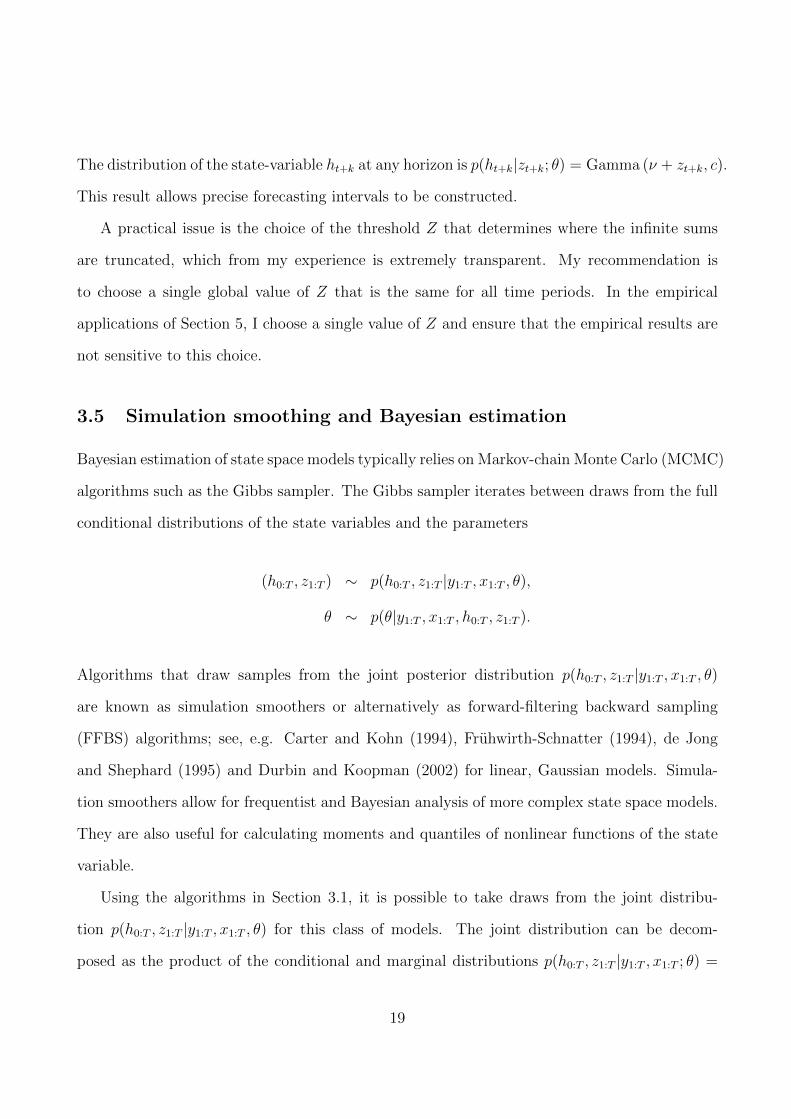
Figure 2 contains filtered and smoothed estimates of the latent frailty factor ht (right graph)

as well as filtered estimates of the instantaneous default intensity (left) given by htτ exp (xitβ).

This default intensity has been scaled up by 1000 and plotted along with the observed number

of defaults yit per day. The frailty factor ht demonstrates considerable variation over the credit

cycle and is a large fraction of the overall default intensity. These moments and quantiles

of the marginal filtering and smoothing distributions are calculated using the full conditional

distributions (14) and (15).

5.2 Stochastic volatility application

Next, I consider the stochastic volatility model (16). I estimate the model on three datasets

including the S&P 500 index, the MSCI-Emerging Markets Asia index, and the Euro-to-U.S.

dollar exchange rate. The first two series were downloaded from Bloomberg and the latter series

was taken from the Board of Governors of the Federal Reserve. All series are from January

3rd, 2000 to December 16th, 2011 making for 3009, 3118, and 3008 observations for each

series, respectively. Starting values for the parameters of the variance (φ, ν, c) were obtained

by matching the unconditional mean, variance, and persistence of average squared returns to

26

2000 2002 2004 2006 2008 2010 20120

1

2

3

4

5

6

7

8

9

10

11Observed defaults and the filtered default itensity

2000 2002 2004 2006 2008 2010 20120

0.002

0.004

0.006

0.008

0.01

0.012

Filtered and smoothed estimate of ht

SmoothedFiltered

Figure 2: Estimation results for the Cox process model with frailty factor from January 30, 1999 through

August 6, 2012. Left: observed (daily) defaults and 1000 times the filtered intensity htτ exp (xitβ). Right:

filtered and smoothed estimates of the frailty state variable ht.

the unconditional distribution. The Feller condition ν > 1 as well as the constraints 0 < φ < 1

and c > 0 were imposed throughout the estimation. For simplicity, I set β = 0 in (16).

The observation and transition densities (17) and (18) are functions of the modified Bessel

function of the second kind Kν (x). In the online appendix, I discuss how to evaluate this

function in a numerically stable manner. The full conditional distributions needed to calculate

the marginal filtering and smoothing estimates are (19) and (20), respectively. The initial

distributions including p(z2|y1; θ) and the log-likelihood contribution p(y1; θ) are available in

the on-line appendix.

Estimates of the parameters of the model as well as robust standard errors are reported

in Table 3. The implied parameters of the continuous-time model are also reported in Table

3 assuming a discretization step size of τ = 1256

. For all series, the risk premium parameters

γ are estimated to be negative and significant implying that the distribution of returns are

negatively skewed. Estimates of the autocorrelation parameter φ for the S&P500 and MSCI

series are slightly smaller than is often reported in the literature for log-normal SV models.

The dynamics of volatility for the Euro/$ series is substantially different than the other series.

27

Table 3: Maximum likelihood estimates for the stochastic volatility model.

µ γ φ c ν θh κ σ2h log-like

S&P500 0.102 -0.061 0.988 0.015 1.539 1.815 3.168 7.470 -4542.1(0.021) (0.020) (0.005) (0.006) (0.221)

MSCI-EM-ASIA 0.250 -0.115 0.978 0.024 1.963 2.115 5.736 12.364 -5213.2(0.081) (0.040) (0.013) (0.008) (0.511)

Euro/$ 0.073 -0.148 0.994 0.0007 3.740 0.442 1.489 0.359 -2862.2(0.051) (0.089) (0.003) (0.0002) (0.384)

Maximum likelihood estimates of the parameters θ = (µ, γ, φ, c, ν) of the stochastic volatility model on threedata sets of daily returns. The series are the S&P500, the MSCI emerging markets Asia index, and theEURO-$ exchange rate. The data cover January 3, 2000 to December 16, 2011. Asymptotic robust standarderrors are reported in parenthesis. The continuous-time parameters are reported for intervals τ = 1

256 .

The mean θh of volatility is much lower and the volatility is more persistent.

Figure 3 contains output from the estimated model for the S&P500 series. The top left

panel is a plot of the filtered and smoothed estimates of the volatility√ht over the sample

period. The estimates are consistent with what one would expect from looking at the raw

return series. There are large increases in volatility during the U.S. financial crisis of 2008

followed by another recent spike in volatility during the European debt crisis.

To provide some information on how the truncation parameter Z impacts the estimates,

the top right panel of Figure 3 is a plot of the marginal filtering distributions for the discrete

mixing variable p(zt|y1:t; θ) on three different days. The three distributions that are pictured are

representative of the distribution p(zt|y1:t; θ) during low (6/27/2007), medium (10/2/2008), and

high volatility (12/1/2008) periods. The distribution of zt for the final date (12/1/2008) was

chosen because it is the day at which the mean of zt is estimated to be the largest throughout

the sample. Consequently, it is the distribution where the truncation will have the largest

impact. This time period also corresponds to the largest estimated value of the variance ht.

The graph illustrates visually that the impact of truncating the distribution is negligible as the

truncation point is far into the tails of the distribution.

28

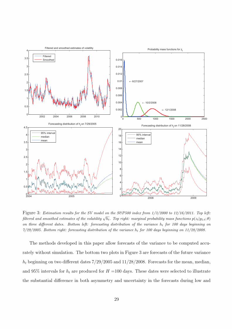
2002 2004 2006 2008 20100

0.5

1

1.5

2

2.5

3

3.5

4Filtered and smoothed estimates of volatility

Filtered

Smoothed

0 500 1000 1500 2000 25000

0.002

0.004

0.006

0.008

0.01

0.012

0.014

0.016

Probability mass functions for zt

← 6/27/2007

← 10/2/2008

← 12/1/2008

2004 20050

0.5

1

1.5

2

2.5

3

3.5

4

4.5

Forecasting distribution of ht on 7/29/2005

95% interval

median

mean

2008 20090

2

4

6

8

10

12

14

16

18

20

Forecasting distribution of ht on 11/28/2008

95% interval

median

mean

Figure 3: Estimation results for the SV model on the S&P500 index from 1/3/2000 to 12/16/2011. Top left:

filtered and smoothed estimates of the volatility√ht. Top right: marginal probability mass functions p(zt|y1:t; θ)

on three different dates. Bottom left: forecasting distribution of the variance ht for 100 days beginning on

7/29/2005. Bottom right: forecasting distribution of the variance ht for 100 days beginning on 11/28/2008.

The methods developed in this paper allow forecasts of the variance to be computed accu-

rately without simulation. The bottom two plots in Figure 3 are forecasts of the future variance

ht beginning on two different dates 7/29/2005 and 11/28/2008. Forecasts for the mean, median,

and 95% intervals for ht are produced for H =100 days. These dates were selected to illustrate

the substantial difference in both asymmetry and uncertainty in the forecasts during low and

29

high periods of volatility. When volatility is low (7/29/2005), the forecasting distribution of ht

is highly asymmetric and the mean and median of the distribution differ in economically im-

portant ways. Conversely, when volatility is high (11/28/2008), the distribution of the variance

is roughly normally distributed. The difference in width of the 95% error bands between the

two dates also illustrates how much more uncertainty exists in the financial markets during a

crisis.

6 Conclusion

In this paper, I developed methods for filtering, smoothing, likelihood evaluation, and simula-

tion smoothing for a class of non-Gaussian state space models that includes stochastic volatility,

stochastic intensity, stochastic duration as well as many others. The approach is based on the

insight that it is possible to integrate out the latent variance analytically leaving only a discrete

mixture variable. The discrete variable is defined over the set of non-negative integers but for

practical purposes it is possible to approximate the distributions involved by a finite-dimensional

Markov switching model. Consequently, the log-likelihood function can be computed exactly

using standard algorithms for Markov-switching models. Filtered and smoothed estimates of

the continuous-valued state variable can easily be computed as a by-product.

There are several extensions to this paper that would be interesting for future research. A

multivariate (vector) autoregressive gamma process has been recently developed in Creal and

Wu (2015). In this case, the dynamics of the state variables follow a vector autoregressive

gamma process and their transition density is a vector non-central gamma distribution. Using

their results, it is possible to expand the dimension of the state variables ht and allow the

observation density p(yt|ht, xt; θ) to depend on an H × 1 vector of state variables ht. This

extension allows for models with richer dynamics for the state variables.

30

7 Acknowledgements

I would like to thank two anonymous referees, Alan Bester, Chris Hansen, Robert Gramacy,

Siem Jan Koopman, Neil Shephard, and Jing Cynthia Wu as well as seminar participants at the

Triangle Econometrics Workshop (UNC Chapel Hill), Univ. of Washington, Federal Reserve

Bank of Atlanta, Northwestern (Kellogg), Erasmus Univ. Rotterdam, and SNDE conference

(Milan) and SoFIE conference (Singapore) for their helpful comments.

References

Bansal, R. and A. Yaron (2004). Risks for the long run: a potential explanation of asset

pricing puzzles. The Journal of Finance 59 (4), 1481–1509.

Barndorff-Nielsen, O. E. and N. Shephard (2012). Basics of Levy processes. Working paper,

Oxford-Man Institute, University of Oxford.

Baum, L. E. and T. P. Petrie (1966). Statistical inference for probabilistic functions of finite

state Markov chains. The Annals of Mathematical Statistics 37 (1), 1554–1563.

Baum, L. E., T. P. Petrie, G. Soules, and N. Weiss (1970). A maximization technique oc-

curring in the statistical analysis of probabilistic functions of finite state Markov chains.

The Annals of Mathematical Statistics 41 (6), 164–171.

Cappe, O., E. Moulines, and T. Ryden (2005). Inference in Hidden Markov Models. New

York: Springer Press.

Carlin, B., N. G. Polson, and D. S. Stoffer (1992). A Monte Carlo approach to nonnormal

and nonlinear state-space modeling. Journal of the American Statistical Association 87,

493–500.

Carter, C. K. and R. Kohn (1994). On Gibbs sampling for state space models.

Biometrika 81 (3), 541–553.

31

Chaleyat-Maurel, M. and V. Genon-Catalot (2006). Computable infinite-dimensional filters

with applications to discretized diffusion processes. Stochastic Processes and their Appli-

cations 116, 1447–1467.

Chan, K. S. and J. Ledolter (1995). Monte Carlo EM estimation for time series models

involving counts. Journal of the American Statistical Association 90 (429), 242–252.

Chen, R. and J. S. Liu (2000). Mixture Kalman filters. Journal of the Royal Statistical Society,

Series B 62 (3), 493–508.

Chib, S. (1996). Calculating posterior distributions and modal estimates in Markov mixture

models. Journal of Econometrics 75 (1), 79–97.

Chopin, N. (2004). Central limit theorem for sequential Monte Carlo and its application to

Bayesian inference. The Annals of Statistics 32 (6), 2385–2411.

Cox, D. R. (1955). Some statistical methods connected with series of events. Journal of the

Royal Statistical Society, Series B 17 (2), 129–164.

Cox, J. C., J. E. Ingersoll, and S. A. Ross (1985). A theory of the term structure of interest

rates. Econometrica 53 (2), 385–407.

Creal, D. D. (2012). A survey of sequential Monte Carlo methods for economics and finance.

Econometric Reviews 31 (3), 245–296.

Creal, D. D., S. J. Koopman, and A. Lucas (2013). Generalized autoregressive score models

with applications. Journal of Applied Econometrics 28 (5), 777–795.

Creal, D. D. and J. C. Wu (2015). Estimation of affine term structure models with spanned

or unspanned stochastic volatility. Journal of Econometrics 185 (1), 60–81.

de Jong, P. and N. Shephard (1995). The simulation smoother for time series models.

Biometrika 82 (2), 339–350.

32

Devroye, L. (2002). Simulating Bessel random variables. Statistics & Probability Let-

ters 57 (3), 249–257.

Doucet, A. and A. J. Johansen (2011). A tutorial on particle filtering and smoothing: Fifteen

years later. In D. C. et B. Rozovsky (Ed.), Handbook of Nonlinear Filtering. Oxford

University Press.

Duffie, D. (2011). Measuring Corporate Default Risk. Princeton, NJ: Oxford University Press.

Duffie, D., A. Eckner, G. Horel, and L. Saita (2009). Frailty correlated default. The Journal

of Finance 64 (5), 2089–2123.

Duffie, D., D. Filipovic, and W. Schachermayer (2003). Affine processes and applications in

finance. Annals of Applied Probability 13, 984–1053.

Duffie, D. and K. J. Singleton (2003). Credit Risk. Princeton, NJ: Princeton University Press.

Durbin, J. and S. J. Koopman (2002). A simple and efficient simulation smoother for state

space time series analysis. Biometrika 89 (3), 603–616.

Durbin, J. and S. J. Koopman (2012). Time Series Analysis by State Space Methods (2 ed.).

Oxford, UK: Oxford University Press.

Engle, R. F. and J. R. Russell (1998). Autoregressive conditional duration: a new model for

irregularly spaced transaction data. Econometrica 66 (5), 1127–1162.

Feller, W. S. (1951). Two singular diffusion problems. Annals of Mathematics 54 (1), 173–182.

Fruhwirth-Schnatter, S. (1994). Data augmentation and dynamic linear models. Journal of

Time Series Analysis 15 (2), 183–202.

Fruhwirth-Schnatter, S. (2006). Finite Mixture and Markov Switching Models. New York,

NY: Springer Press.

Gammerman, D., T. R. dos Santos, and G. C. Franco (2013). A non-Gaussian family of state-

space models with exact marginal likelihood. Journal of Time Series Analysis 34 (6),

33

625–645.

Gourieroux, C. and J. Jasiak (2006). Autoregressive gamma processes. Journal of Forecast-

ing 25 (2), 129–152.

Gradshteyn, I. S. and I. M. Ryzhik (2007). Table of Integrals, Series, and Products. Amster-

dam, The Netherlands: Academic Press.

Hamilton, J. D. (1986). A standard error for the estimated state vector of a state-space

model. Journal of Econometrics 33 (3), 387–397.

Hamilton, J. D. (1989). A new approach to the econometric analysis of nonstationary time

series and the business cycle. Econometrica 57 (2), 357–384.

Hamilton, J. D. (1994). Time Series Analysis. Princeton, NJ: Princeton University Press.

Harvey, A. C. (1989). Forecasting, structural time series models and the Kalman filter. Cam-

bridge, UK: Cambridge University Press.

Hautsch, N. (2011). Econometrics of Financial High-Frequency Data. New York, NY:

Springer Press.

Heston, S. L. (1993). A closed-form solution for options with stochastic volatility with appli-

cations to bond and currency options. The Review of Financial Studies 6 (2), 327–343.

Kalman, R. (1960). A new approach to linear filtering and prediction problems. Journal of

Basic Engineering, Transactions of the ASME 82 (1), 35–46.

Klass, M., N. de Freitas, and A. Doucet (2005). Toward practical N2 Monte Carlo: the

marginal particle filter. Proceedings of the 21st Conference on Uncertainty in Artificial

Intelligence.

Koopman, S. J., A. Lucas, and A. Monteiro (2008). The multi-state latent factor intensity

model for credit rating transitions. Journal of Econometrics 142 (1), 399–424.

34

Marsaglia, G., W. W. Tsang, and J. Wang (2004). Fast generation of discrete random vari-

ables. Journal of Statistical Software 11 (3), 1–11.

McNeil, A. J., R. Frey, and P. Embrechts (2005). Quantitative Risk Management. Princeton,

NJ: Princeton University Press.

Schweppe, F. C. (1965). Evaluation of likelihood functions for Gaussian signals. IEEE Trans-

actions on Information Theory 11, 61–70.

Shephard, N. (1994). Location scale models. Journal of Econometrics 60, 181–202.

Sichel, H. S. (1974). On a distribution representing sentence-length in written prose. Journal

of the Royal Statistical Society, Series A 135 (1), 25–34.

Sichel, H. S. (1975). On a distribution law for word frequencies. Journal of the American

Statistical Association 70 (350), 542–547.

Smith, R. L. and J. E. Miller (1986). A non-Gaussian state space model and application to

prediction of records. Journal of the Royal Statistical Society, Series B 48 (1), 79–88.

Uhlig, H. (1994). Vector autoregressions with stochastic volatility. Econometrica 63 (1), 59–

73.

van den Berg, G. J. (2001). Duration models: specification, identification and multiple du-

rations. In J. J. Heckman and E. E. Leamer (Eds.), Handbook of Econometrics, Vol 1,

Number 5. Elsevier.

Vidoni, P. (1999). Exponential family state space models based on a conjugate latent process.

Journal of the Royal Statistical Society, Series B 61 (1), 213–221.

West, M. and J. Harrison (1997). Bayesian Forecasting and Dynamic Models (Second ed.).

New York, NY: Springer.

White, H. L. (1982). Maximum likelihood estimation of misspecified models. Economet-

rica 50 (1), 1–25.

35