Some properties of Likelihood Ratio Tests in Linear Mixed Models

Ciprian M. Crainiceanu∗ David Ruppert† Timothy J. Vogelsang‡

September 19, 2003

Abstract

We calculate the finite sample probability mass-at-zero and the probability of underesti-mating the true ratio between random effects variance and error variance in a LMM with onevariance component. The calculations are expedited by simple matrix diagonalization tech-niques. One possible application is to compute the probability that the log of the likelihoodratio (LRT), or residual likelihood ratio (RLRT), is zero. The large sample chi-square mixtureapproximation to the distribution of the log-likelihood ratio, using the usual asymptotic theoryfor when a parameter is on the boundary, has been shown to be poor in simulations studies. Alarge part of the problem is that the finite-sample probability that the LRT or RLRT statistic iszero is larger than 0.5, its value under the chi-square mixture approximation. Our calculationsexplain these empirical results. Another application is to show why standard asymptotic resultscan fail even when the parameter under the null is in the interior of the parameter space.

This paper focuses on LMMs with one variance component because we have developed a veryrapid algorithm for simulating finite-sample distributions of the LRT and RLRT statistics forthis case. This allows us to compare finite-sample distributions with asymptotic approximations.The main result is the asymptotic approximation are often poor, and this results suggests thatasymptotics be used with caution, or avoided altogether, for any LMM regardless of whether ithas one variance component or more. For computing the distribution of the test statistics werecommend our algorithm for the case of one variance component and the bootstrap in othercases.

Short title: Properties of (R)LRT

Keywords: Effects of dependence, Penalized splines, Testing polynomial regression.

∗Department of Statistical Science, Cornell University, Malott Hall, NY 14853, USA. E-mail: cmc59@cornell.edu†School of Operational Research and Industrial Engineering, Cornell University, Rhodes Hall, NY 14853, USA.

E-mail: ruppert@orie.cornell.edu‡Departments of Economics and Statistics, Cornell University, Uris Hall, NY 14853-7601, USA. E-

mail:tjv2@cornell.edu

1 INTRODUCTION

This work was motivated by our research in testing parametric regression models versus non-

parametric alternatives. It is becoming more widely appreciated that penalized splines and other

penalized likelihood models can be viewed as LMMs and the fitted curves as BLUPs (e.g., Brum-

back, Ruppert, and Wand, 1999). In this framework the smoothing parameter is a ratio of variance

components and can be estimated by ML or REML. REML is often called generalized maximum

likelihood (GML) in the smoothing spline literature. Within the random effects framework, it is

natural to consider likelihood ratio tests and residual likelihood ratio tests, (R)LRTs, about the

smoothing parameter. In particular, testing whether the smoothing parameter is zero is equiva-

lent to testing for polynomial regression versus a general alternative modeled by penalized splines.

These null hypotheses are also equivalent to the hypothesis that a variance component is zero.

LRTs for null variance components are non-standard for two reasons. First, the null value of the

parameter is on the boundary of the parameter space. Second, the data are dependent, at least

under the alternative hypothesis.

The focus of our research is on the finite sample distributions of (R)LRT statistics, and the

asymptotic distributions are derived as limits of the finite sample distributions in order to compare

the accuracy of various types of asymptotics. For example, for balanced one-way ANOVA we

compare asymptotics with a fixed number of samples and the number of observations per sample

going to infinity with the opposite case of the number of samples tending to infinity with the number

of observations per sample fixed. Our major results are

a. The usual asymptotic theory for standard or boundary problems provides accurate approxi-

mations to finite-sample distributions only when the response vector can be partitioned into

a large number of independent sub-vectors, for all values of the parameters.

b. The asymptotic approximations can be very poor when the number of independent sub-vectors

is small or moderate.

c. Penalized spline models do not satisfy the condition described in point a. and standard asymp-

totic results fail rather dramatically.

The usual asymptotics for testing that a single parameter is at the boundary of its range is

a 50 : 50 mixture of point mass at zero (called χ20) and a χ2

1 distribution. A major reason why

1

the asymptotics fail to produce accurate finite-sample approximations is that the finite-sample

probability mass at χ20 is substantially greater than 0.5, especially for the LRT but even for the

RLRT. This paper studies the amount of probability mass at 0 for these test statistics. However,

our methods are sufficiently powerful that the finite-sample distribution of the LRT and RLRT

statistics, conditional on being zero, can also be derived. These distributions are studied in a later

paper (Crainiceanu and Ruppert, 2003).

Our work is applicable to most LMMs with a single random effects variance component, not

only to penalized likelihood models. We study LMMs with only a single variance component

for tractability. When there is only one variance component, the distributions of the LRT and

RLRT statistics can be simplified in such a way that simulation of these distributions is extremely

rapid. Although our results do not apply to LMMs with more than one variance component,

they strongly suggest that asymptotic approximations be used with great caution for such models.

Since asymptotic approximations are poor for LMMs with one variance, it is unlikely that they

satisfactory in general when there is more than one variance components.

Consider the following LMM

Y = Xβ + Zb + ε, E[

bε

]=

[0K

0n

], Cov

[bε

]=

[σ2

bΣ 00 σ2

ε IK

], (1)

where Y is an n-dimensional response vector, 0K is a K-dimensional column of zeros, Σ is a known

K ×K-dimensional, β is a p-dimensional vector of parameters corresponding to fixed effects, b is

a K-dimensional vector of exchangeable random effects, and (b, ε) is a normal distributed random

vector. Under these conditions it follows that E(Y ) = Xβ and Cov(Y ) = σ2ε V λ, where λ = σ2

b/σ2ε

is the ratio between the variance of random effects b and the variance of the error variables ε,

V λ = In + λZΣZT , and n is the size of the vector Y of the response variable. Note that σ2b = 0

if and only if λ = 0 and the parameter space for λ is [0,∞).

The LMM described by equation (1) contains standard regression fixed effects Xβ specifying the

conditional response mean and random effects Zb that account for correlation. We are interested

in testing

H0 : λ = λ0 vs. HA : λ ∈ [0,∞) \ {λ0} , (2)

where λ0 ∈ [0,∞).

Consider the case λ0 = 0 (σ2b = 0) when the parameter is on the boundary of the parameter

space under the null. Using non-standard asymptotic theory developed by Self and Liang (1987)

2

for independent data, one may be tempted to conclude that the finite samples distribution of the

(R)LRT could be approximated by a 0.5χ20 + 0.5χ2

1 mixture. Here χ2k is the chi-square distribution

with k degrees of freedom and χ20 means point probability mass at 0. However, results of Self and

Liang (1987) require independence for all values of the parameter. Because the response variable Y

in model (1) is not a vector of independent random variables, this theory does not apply. Stram and

Lee (1994) showed that the Self and Liang result can still be applied to testing for the zero variance

of random effects in LMMs in which the response variable Y can be partitioned into independent

vectors and the number of independent subvectors tends to infinity.

In a simulation study for a related model, Pinheiro and Bates (2000) found that a 0.5χ20 +0.5χ2

1

mixture distribution approximates well the finite sample distribution of RLRT, but that a 0.65χ20 +

0.35χ21 mixture approximates better the finite sample distribution of LRT. A case where it has

been shown that the asymptotic mixture probabilities differ from 0.5χ20 + 0.5χ2

1 is regression with

a stochastic trend analyzed by Shephard and Harvey (1990) and Shephard (1993). They consider

the particular case of model (1) where the random effects b are modeled as a random walk and

show that the asymptotic mass at zero can be as large as 0.96 for LRT and 0.65 for RLRT.

For the case when λ0 > 0 we show that the distribution of the (RE)ML estimator of λ has

mass at zero. Therefore, even when the parameter is in the interior of the parameter space under

the null, the asymptotic distributions of the (R)LRT statistics are not χ21. We also calculate the

probability of underestimating the true parameter λ0 and show that in the penalized spline models

this probability is larger than 0.5, showing that (RE)ML criteria tend to oversmooth the data. This

effect is more severe for ML than for REML.

Section 6.2 of Khuri, Mathew, and Sinha (1998) studies mixed models with one variance com-

ponent. (They consider the error variance as a variance component so they call this case “two

variance components.”) In their Theorem 6.2.2, they derive the LBI (locally best invariant) test of

H0: λ = 0 which rejects for large values of

F ∗ =eT ZΣZT e

eT e, (3)

where e = {I − X(XT X)−1X}Y is the residual vector when fitting the null model. A test is

LBI if among all invariant tests it maximizes power in some neighborhood of the null hypothesis.

Notice that the denominator of (3) is, except for a scale factor, the estimator of σ2 under the null

hypothesis and will be inflated by deviations from the null. This suggests that the test might have

3

low power at alternatives far from the null.

Khuri (1994) studies the probability in a LMM that a linear combination of independent mean

squares is negative. For certain balanced models, there is an estimator of σ2b of this form such that

this estimator is negative if and only if the (R)LRT statistic is zero; see, for example, Sections 3.7

and 3.8 of Searle, Casella, and McCulloch (1992). However, in general Khuri’s results to do apply

to our problem.

2 SPECTRAL DECOMPOSITION OF (R)LRTn

Consider maximum likelihood estimation (MLE) for model (1). Twice the log-likelihood of Y given

the parameters β, σ2ε , and λ is, up to a constant that does not depend on the parameters,

L(β, σ2ε , λ) = −n log σ2

ε − log |V λ| −(Y −Xβ)T V −1

λ (Y −Xβ)σ2

ε

. (4)

Residual or restricted maximum likelihood (REML) was introduced by Patterson and Thompson

(1971) to take into account the loss in degrees of freedom due to estimation of β parameters and

thereby to obtain unbiased variance components estimators. REML consists of maximizing the

likelihood function associated with n−p linearly independent error contrasts. It makes no difference

which n− p contrasts are used because the likelihood function for any such set differs by no more

than an additive constant (Harville, 1977). For the LMM described in equation (1), twice the

residual log-likelihood was derived by Harville (1974) and is

REL(σ2ε , λ) = −(n− p) log σ2

ε − log |V λ| − log(XTV λX)− (Y −Xβ̂λ)T V −1λ (Y −Xβ̂λ)

σ2ε

, (5)

where β̂λ = (XTV −1λ X)−1(XTV −1

λ Y ) maximizes the likelihood as a function of β for a fixed

value of λ. The (R)LRT statistics for testing hypotheses described in (2) are

LRTn = supHA∪H0

L(β, σ2ε , λ)− sup

H0

L(β, σ2ε , λ) , RLRTn = sup

HA∪H0

REL(σ2ε , λ)− sup

H0

REL(σ2ε , λ) (6)

Denote by µs,n and ξs,n the K eigenvalues of the K×K matrices Σ1/2ZT P 0ZΣ1/2 and Σ1/2ZT ZΣ1/2

respectively, where P 0 = In −X(XT X)−1XT . Crainiceanu and Ruppert (2003) showed that if

λ0 is the true value of the parameter then

LRTnD= sup

λ∈[0,∞)

[n log

{1 +

Nn(λ, λ0)Dn(λ, λ0)

}−

K∑

s=1

log(

1 + λξs,n

1 + λ0ξs,n

)], (7)

4

RLRTnD= sup

λ∈[0,∞)

[(n− p) log

{1 +

Nn(λ, λ0)Dn(λ, λ0)

}−

K∑

s=1

log(

1 + λµs,n

1 + λ0µs,n

)], (8)

where “D=” denotes equality in distribution,

Nn(λ, λ0) =K∑

s=1

(λ− λ0)µs,n

1 + λµs,nw2

s , Dn(λ, λ0) =K∑

s=1

1 + λ0µs,n

1 + λµs,nw2

s +n−p∑

s=K+1

w2s ,

and ws, for s = 1, . . . , n − p, are independent N(0, 1). These null finite sample distributions are

easy to simulate (Crainiceanu and Ruppert, 2003).

3 PROBABILITY MASS AT ZERO OF (R)LRT

Denote by f(·) and g(·) the functions to be maximized in equations (7) and (8) respectively. Note

that the probability mass at zero for LRTn or RLRTn equals the probability that the function f(·)or g(·) has a global maximum at λ = 0. For a given sample size we compute the exact probability

of having a local maximum of the f(·) and g(·) at λ = 0. This probability is an upper bound for the

probability of having a global maximum at zero but, as we will show using simulations, it provides

an excellent approximation.

The first order condition for having a local maximum of f(·) at λ = 0 is f ′(0) ≤ 0 , where the

derivative is taken from the right. The finite sample probability of a local maximum at λ = 0 for

ML, when λ0 is the true value of the parameter, is

P

{ ∑Ks=1(1 + λ0µs,n)µs,nw2

s∑Ks=1(1 + λ0µs,n)w2

s +∑n−p

s=K+1 w2s

≤ 1n

K∑

s=1

ξs,n

}, (9)

where µs,n and ξs,n are the eigenvalues of the K×K matrices Σ1/2ZT P 0ZΣ1/2 and Σ1/2ZT ZΣ1/2

respectively, and ws are i.i.d. N(0,1) random variables. If λ0 = 0 then the probability of a local

maximum at λ = 0 is

P

{∑Ks=1 µs,nw2

s∑n−ps=1 w2

s

≤ 1n

K∑

s=1

ξs,n

}. (10)

Using similar derivations for REML the probability mass at zero when λ = λ0 is

P

{ ∑Ks=1(1 + λ0µs,n)µs,nw2

s∑Ks=1(1 + λ0µs,n)w2

s +∑n−p

s=K+1 w2s

≤ 1n− p

K∑

s=1

µs,n

}, (11)

and, in the particular case when λ0 = 0, the probability of a local maximum at λ = 0 is

P

{∑Ks=1 µs,nw2

s∑n−ps=1 w2

s

≤ 1n− p

K∑

s=1

µs,n

}. (12)

5

Once the eigenvalues µs,n and ξs,n are computed explicitly or numerically, these probabilities

can be simulated. Algorithms for computation of the distribution of a linear combination of χ21

random variables developed by Davies (1980) or Farebrother (1990) could also be used, but we used

simulations because they are simple, accurate, and easier to program. For K = 20 we obtained 1

million simulations in 1 minute (2.66GHz, 1Mb RAM).

Probabilities in equations (9) and (11) are the probabilities that λ = 0 is a local maximum and

provide approximations of the probabilities that λ = 0 is a global maximum. The latter is equal to

the finite sample probability mass at zero of the (R)LRT and of (RE)ML estimator of λ when the

true value of the parameter is λ0.

For every value λ0 we can compute the probability of a local maximum at λ = 0 for (RE)ML

using the corresponding equation (9) or (11). However, there is no close form for the probability

of a global maximum at λ = 0 and we use simulation of the finite sample distributions of (R)LRTn

statistics described in equations (7) or (8). In sections 5 and 6 we show that that there is close

agreement between the probability of a local and global maximum at λ = 0 for two examples:

balanced one-way ANOVA and penalized spline models.

4 PROBABILITY OF UNDERESTIMATING THE SIGNAL-TO-NOISE PARAM-ETER

Denote by λ̂ML and λ̂1ML the global and the first local maximum of f(·), respectively. Define λ̂REML

and λ̂1REML similarly using g(·). When λ0 is the true value of the signal-to-noise parameter,

P(λ̂1

ML < λ0

)≥ P

{∂

∂λf(λ)

∣∣∣∣λ=λ0

< 0

}= P

{K∑

s=1

cs,n(λ0)w2s <

∑n−ps=1 w2

s

n

}, (13)

where

cs,n(λ0) =µs,n

1 + λ0µs,n

/ K∑

s=1

ξs,n

1 + λ0ξs,n.

Similarly, for REML we obtain

P(λ̂1

REML < λ0

)≥ P

{∂

∂λg(λ)

∣∣∣∣λ=λ0

< 0

}= P

{K∑

s=1

ds,n(λ0)w2s <

∑n−ps=1 w2

s

n− p

}, (14)

where

ds,n(λ0) =µs,n

1 + λ0µs,n

/ K∑

s=1

µs,n

1 + λ0µs,n.

6

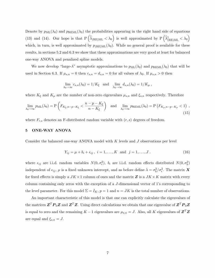
Denote by pML(λ0) and pREML(λ0) the probabilities appearing in the right hand side of equations

(13) and (14). Our hope is that P(λ̂(RE)ML < λ0

)is well approximated by P

(λ̂1

(RE)ML < λ0

)

which, in turn, is well approximated by p(RE)ML(λ0). While no general proof is available for these

results, in sections 5.2 and 6.3 we show that these approximations are very good at least for balanced

one-way ANOVA and penalized spline models.

We now develop “large-λ” asymptotic approximations to pML(λ0) and pREML(λ0) that will be

used in Section 6.3. If µs,n = 0 then cs,n = ds,n = 0 for all values of λ0. If µs,n > 0 then

limλ0→∞

cs,n(λ0) = 1/Kξ and limλ0→∞

ds,n(λ0) = 1/Kµ ,

where Kξ and Kµ are the number of non-zero eigenvalues µs,n and ξs,n respectively. Therefore

limλ0→∞

pML(λ0) = P(

FKξ,n−p−Kξ<

n− p−Kξ

n−Kξ

)and lim

λ0→∞pREML(λ0) = P

(FKµ,n−p−Kµ < 1

),

(15)

where Fr,s denotes an F-distributed random variable with (r, s) degrees of freedom.

5 ONE-WAY ANOVA

Consider the balanced one-way ANOVA model with K levels and J observations per level

Yij = µ + bi + εij , i = 1, . . . , K and j = 1, . . . , J . (16)

where εij are i.i.d. random variables N(0, σ2ε ), bi are i.i.d. random effects distributed N(0, σ2

b )

independent of εij , µ is a fixed unknown intercept, and as before define λ = σ2b/σ2

ε . The matrix X

for fixed effects is simply a JK×1 column of ones and the matrix Z is a JK×K matrix with every

column containing only zeros with the exception of a J-dimensional vector of 1’s corresponding to

the level parameter. For this model Σ = IK , p = 1 and n = JK is the total number of observations.

An important characteristic of this model is that one can explicitly calculate the eigenvalues of

the matrices ZT P 0Z and ZT Z. Using direct calculations we obtain that one eigenvalue of ZT P 0Z

is equal to zero and the remaining K − 1 eigenvalues are µs,n = J . Also, all K eigenvalues of ZT Z

are equal and ξs,n = J .

7

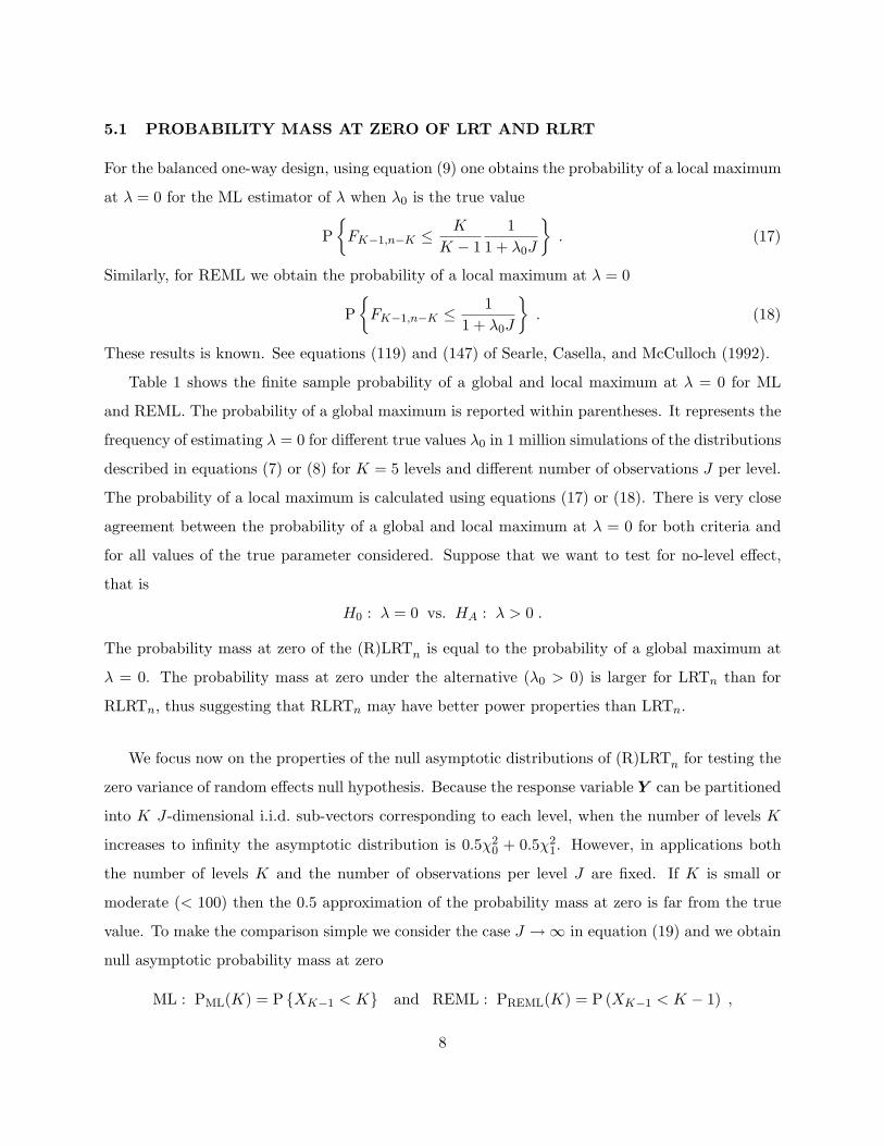
5.1 PROBABILITY MASS AT ZERO OF LRT AND RLRT

For the balanced one-way design, using equation (9) one obtains the probability of a local maximum

at λ = 0 for the ML estimator of λ when λ0 is the true value

P{

FK−1,n−K ≤ K

K − 11

1 + λ0J

}. (17)

Similarly, for REML we obtain the probability of a local maximum at λ = 0

P{

FK−1,n−K ≤ 11 + λ0J

}. (18)

These results is known. See equations (119) and (147) of Searle, Casella, and McCulloch (1992).

Table 1 shows the finite sample probability of a global and local maximum at λ = 0 for ML

and REML. The probability of a global maximum is reported within parentheses. It represents the

frequency of estimating λ = 0 for different true values λ0 in 1 million simulations of the distributions

described in equations (7) or (8) for K = 5 levels and different number of observations J per level.

The probability of a local maximum is calculated using equations (17) or (18). There is very close

agreement between the probability of a global and local maximum at λ = 0 for both criteria and

for all values of the true parameter considered. Suppose that we want to test for no-level effect,

that is

H0 : λ = 0 vs. HA : λ > 0 .

The probability mass at zero of the (R)LRTn is equal to the probability of a global maximum at

λ = 0. The probability mass at zero under the alternative (λ0 > 0) is larger for LRTn than for

RLRTn, thus suggesting that RLRTn may have better power properties than LRTn.

We focus now on the properties of the null asymptotic distributions of (R)LRTn for testing the

zero variance of random effects null hypothesis. Because the response variable Y can be partitioned

into K J-dimensional i.i.d. sub-vectors corresponding to each level, when the number of levels K

increases to infinity the asymptotic distribution is 0.5χ20 + 0.5χ2

1. However, in applications both

the number of levels K and the number of observations per level J are fixed. If K is small or

moderate (< 100) then the 0.5 approximation of the probability mass at zero is far from the true

value. To make the comparison simple we consider the case J →∞ in equation (19) and we obtain

null asymptotic probability mass at zero

ML : PML(K) = P {XK−1 < K} and REML : PREML(K) = P (XK−1 < K − 1) ,

8

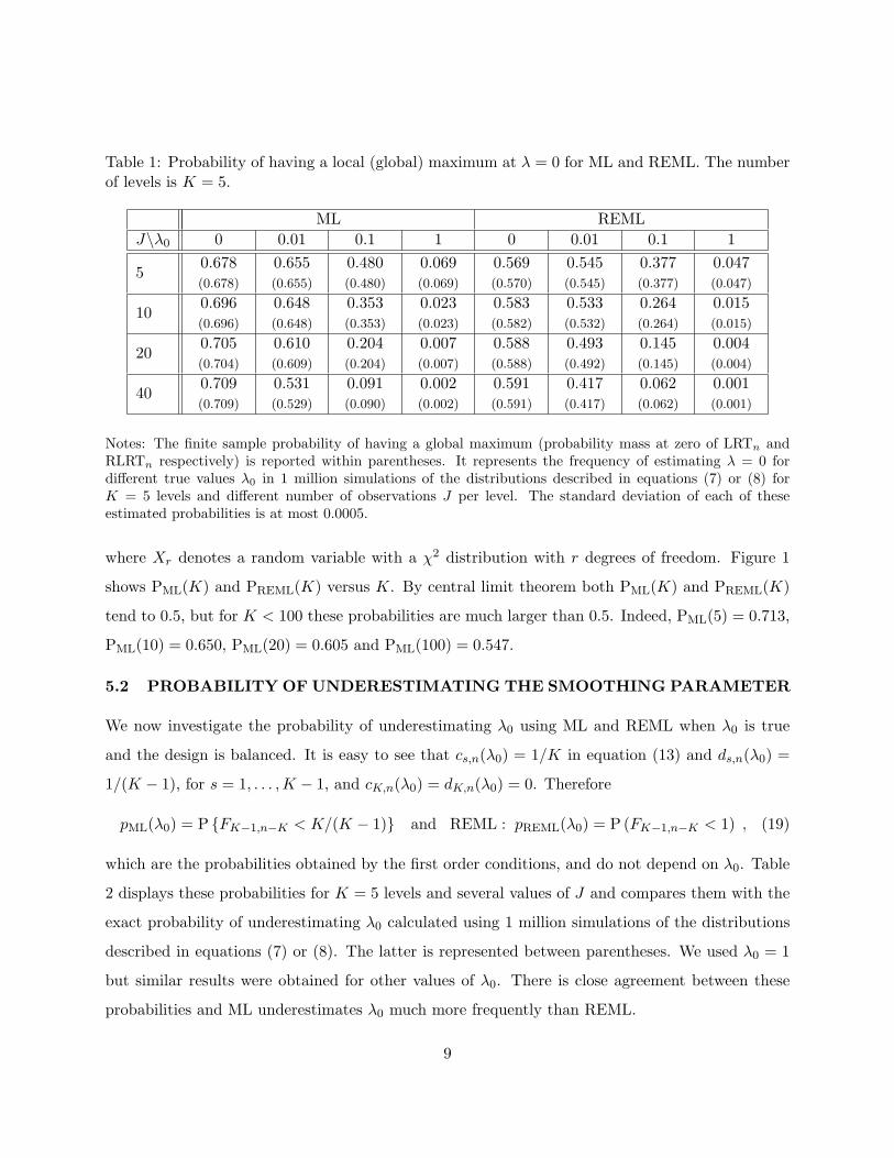
Table 1: Probability of having a local (global) maximum at λ = 0 for ML and REML. The numberof levels is K = 5.

ML REMLJ\λ0 0 0.01 0.1 1 0 0.01 0.1 1

50.678(0.678)

0.655(0.655)

0.480(0.480)

0.069(0.069)

0.569(0.570)

0.545(0.545)

0.377(0.377)

0.047(0.047)

100.696(0.696)

0.648(0.648)

0.353(0.353)

0.023(0.023)

0.583(0.582)

0.533(0.532)

0.264(0.264)

0.015(0.015)

200.705(0.704)

0.610(0.609)

0.204(0.204)

0.007(0.007)

0.588(0.588)

0.493(0.492)

0.145(0.145)

0.004(0.004)

400.709(0.709)

0.531(0.529)

0.091(0.090)

0.002(0.002)

0.591(0.591)

0.417(0.417)

0.062(0.062)

0.001(0.001)

Notes: The finite sample probability of having a global maximum (probability mass at zero of LRTn andRLRTn respectively) is reported within parentheses. It represents the frequency of estimating λ = 0 fordifferent true values λ0 in 1 million simulations of the distributions described in equations (7) or (8) forK = 5 levels and different number of observations J per level. The standard deviation of each of theseestimated probabilities is at most 0.0005.

where Xr denotes a random variable with a χ2 distribution with r degrees of freedom. Figure 1

shows PML(K) and PREML(K) versus K. By central limit theorem both PML(K) and PREML(K)

tend to 0.5, but for K < 100 these probabilities are much larger than 0.5. Indeed, PML(5) = 0.713,

PML(10) = 0.650, PML(20) = 0.605 and PML(100) = 0.547.

5.2 PROBABILITY OF UNDERESTIMATING THE SMOOTHING PARAMETER

We now investigate the probability of underestimating λ0 using ML and REML when λ0 is true

and the design is balanced. It is easy to see that cs,n(λ0) = 1/K in equation (13) and ds,n(λ0) =

1/(K − 1), for s = 1, . . . , K − 1, and cK,n(λ0) = dK,n(λ0) = 0. Therefore

pML(λ0) = P {FK−1,n−K < K/(K − 1)} and REML : pREML(λ0) = P (FK−1,n−K < 1) , (19)

which are the probabilities obtained by the first order conditions, and do not depend on λ0. Table

2 displays these probabilities for K = 5 levels and several values of J and compares them with the

exact probability of underestimating λ0 calculated using 1 million simulations of the distributions

described in equations (7) or (8). The latter is represented between parentheses. We used λ0 = 1

but similar results were obtained for other values of λ0. There is close agreement between these

probabilities and ML underestimates λ0 much more frequently than REML.

9

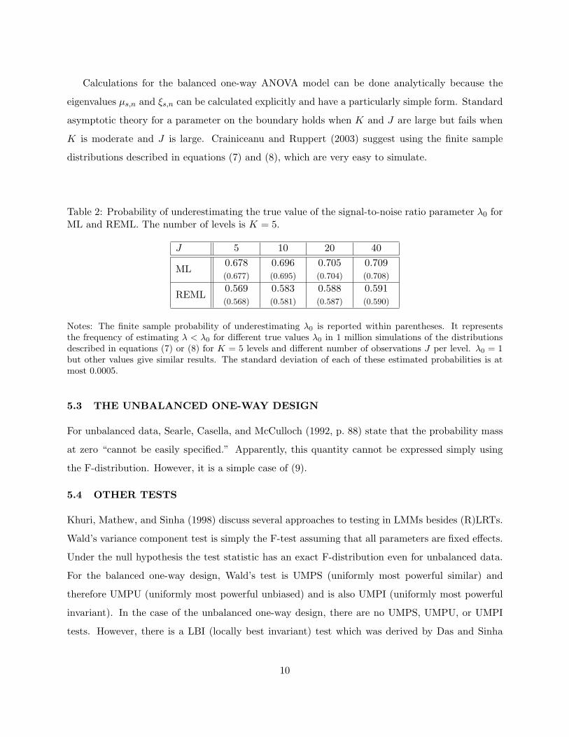
Calculations for the balanced one-way ANOVA model can be done analytically because the

eigenvalues µs,n and ξs,n can be calculated explicitly and have a particularly simple form. Standard

asymptotic theory for a parameter on the boundary holds when K and J are large but fails when

K is moderate and J is large. Crainiceanu and Ruppert (2003) suggest using the finite sample

distributions described in equations (7) and (8), which are very easy to simulate.

Table 2: Probability of underestimating the true value of the signal-to-noise ratio parameter λ0 forML and REML. The number of levels is K = 5.

J 5 10 20 40

ML0.678(0.677)

0.696(0.695)

0.705(0.704)

0.709(0.708)

REML0.569(0.568)

0.583(0.581)

0.588(0.587)

0.591(0.590)

Notes: The finite sample probability of underestimating λ0 is reported within parentheses. It representsthe frequency of estimating λ < λ0 for different true values λ0 in 1 million simulations of the distributionsdescribed in equations (7) or (8) for K = 5 levels and different number of observations J per level. λ0 = 1but other values give similar results. The standard deviation of each of these estimated probabilities is atmost 0.0005.

5.3 THE UNBALANCED ONE-WAY DESIGN

For unbalanced data, Searle, Casella, and McCulloch (1992, p. 88) state that the probability mass

at zero “cannot be easily specified.” Apparently, this quantity cannot be expressed simply using

the F-distribution. However, it is a simple case of (9).

5.4 OTHER TESTS

Khuri, Mathew, and Sinha (1998) discuss several approaches to testing in LMMs besides (R)LRTs.

Wald’s variance component test is simply the F-test assuming that all parameters are fixed effects.

Under the null hypothesis the test statistic has an exact F-distribution even for unbalanced data.

For the balanced one-way design, Wald’s test is UMPS (uniformly most powerful similar) and

therefore UMPU (uniformly most powerful unbiased) and is also UMPI (uniformly most powerful

invariant). In the case of the unbalanced one-way design, there are no UMPS, UMPU, or UMPI

tests. However, there is a LBI (locally best invariant) test which was derived by Das and Sinha

10

(1987). The test statistic, which is given by equation (3) or (4.2.8) of Khuri, Mathew, and Sinha

(1998), is a ratio of quadratic forms in Y so percentiles of its distribution can be found by Davies’s

(1980) algorithm.

6 TESTING POLYNOMIAL REGRESSION VERSUS A NONPARAMETRIC AL-TERNATIVE

In this section we show that nonparametric regression using P-splines is equivalent to a particular

LMM. In this context, the smoothing parameter is the ratio between the random effects and

error variances and testing assumptions about the shape of the regression function is equivalent

to testing hypotheses about the smoothing parameter. We first focus on testing for a polynomial

regression versus a general alternative modeled by penalized splines, which is equivalent to testing

for a zero smoothing parameter (or zero random effects variance). For this hypothesis, we study

the probability mass at zero of the (R)LRTn statistics under the null and alternative hypotheses.

In particular, we show that the null probability mass at zero is much larger than 0.5.

Because in the penalized spline models the data vector cannot be partitioned into more than

one i.i.d. sub-vectors, the Self and Liang assumptions do not hold, but it was an open question

as to whether the results themselves held or not. Our results show that the 0.5 : 0.5 mixture of

χ2 distributions cannot be extended to approximate the finite sample distributions of (R)LRTn

regardless of the number of knots used.

We also investigate the probability of underestimating the true smoothing parameter, which in

the context of penalized spline smoothing is the probability of oversmoothing. We show that first

order results as described in Section 4 provide excellent approximations of the exact probability of

oversmoothing and the probability of oversmoothing with (RE)ML is generally larger than 0.5.

6.1 P-SPLINES REGRESSION AND LINEAR MIXED MODELS

Consider the following regression equation

yi = m (xi) + εi , (20)

where εi are i.i.d. N(0, σ2

ε

)and m(·) is the unknown mean function. Suppose that we are interested

in testing if m(·) is a p-th degree polynomial:

H0 : m (x) = β0 + β1x + . . . + βpxp .

11

To define an alternative that is flexible enough to describe a large class of functions, we consider

the class of regression splines

HA : m(x) = m (x,Θ) = β0 + β1x + . . . + βpxp +

K∑

k=1

bk (x− κk)p+ , (21)

where Θ = (β0, . . . , βp, b1, . . . , bK)T is the vector of regression coefficients, β = (β0, . . . , βp)T is

the vector of polynomial parameters, b = (b1, . . . , bK)T is the vector of spline coefficients, and

κ1 < κ2 < . . . < κK are fixed knots. Following Gray (1994) and Ruppert (2002), we consider a

number of knots that is large enough (e.g. 20) to ensure the desired flexibility. The knots are taken

to be sample quantiles of the x’s such that κk corresponds to probability k/(K + 1). To avoid

overfitting, the criterion to be minimized is a penalized sum of squares

n∑

i=1

{yi −m (xi;Θ)}2 +1λΘT WΘ , (22)

where λ ≥ 0 is the smoothing parameter and W is a positive semi-definite matrix. Denote Y =

(y1, y2, . . . , yn)T , X the matrix having the i-th row Xi = (1, xi, . . . , xpi ) , Z the matrix having the

i-th row Zi ={(xi − κ1)

p+ , (xi − κ2)

p+ , . . . , (xi − κK)p

+

}, and X = [X|Z]. In this paper we focus

on matrices W of the form

W =[

0p+1×p+1 0p+1×K

0K×p+1 Σ−1

],

where Σ is a positive definite matrix and 0ml is an m × l matrix of zeros. This type of matrix

W penalizes the coefficients of the spline basis functions (x − κk)p+ only and will be used in the

remainder of the paper. A standard choice is Σ = IK but other matrices can be used according to

the specific application. If criterion (22) is divided by σ2ε one obtains

1σ2

ε

‖Y −Xβ −Zb‖2 +1

λσ2ε

bTΣ−1b . (23)

Define σ2b = λσ2

ε , consider the vectors γ and β as unknown fixed parameters and the vector b

as a set of random parameters with E(b) = 0 and cov(b) = σ2bΣ. If (bT , εT )T is a normal random

vector and b and ε are independent then one obtains an “equivalent” model representation of the

penalized spline in the form of a LMM (Brumback, Ruppert, and Wand 1999; Ruppert, Wand, and

Carroll, 2003):

Y = Xβ + Zb + ε, cov(

bε

)=

[σ2

bΣ 00 σ2

ε In

]. (24)

12

More specifically, the P-spline model is equivalent to the LMM in the following sense. Given a

fixed value of λ = σ2b/σ2

ε , the P-spline is equal to the BLUP of the regression function in the

LMM. The P-spline model and LMM may differ in how λ is estimated. In the LMM it would

be estimated by ML or REML. In the P-spline model, λ could be determined by cross-validation,

generalized cross-validation or some other method for selecting a smoothing parameter. However,

using ML or REML to select the smoothing parameter is an effective method and we will use it.

There is naturally some concern about modeling a regression function by assuming that (bT , εT )T

is a normal random vector and cov(b) = σ2bΣ. However, under the null hypotheses of interest, b = 0

so this assumption does hold with σ2b = 0. Therefore, this concern is not relevant to the problem

of testing the null hypothesis of a parametric model. One can also view the LMM interpretation

of a P-spline model as a hierarchical Bayesian model and the assumption about (bT , εT )T as part

of the prior. This is analogous to the Bayesian interpretation of smoothing splines pioneered by

Wahba (1978, 1990).

In this context, testing for a polynomial fit against a general alternative described by a P-spline

is equivalent to testing

H0 : λ = 0(σ2

b = 0)

vs. HA : λ > 0(σ2

b > 0)

.

Given the LMM representation of a P-spline model we can define LRTn and RLRTn for testing

these hypotheses as described in Section 2. Because the bi’s have mean zero, σ2b = 0 in H0 is

equivalent to the condition that all coefficients bi of the truncated power functions are identically

zero. These coefficients account for departures from a polynomial.

For the P-spline model, Wald’s variance component test mentioned in Section 5.4 would be

the F-test for testing polynomial regression versus a regression spline viewed as a fixed effects

model. The fit under the alternative would be ordinary least squares. Because there would be no

smoothing, it seems unlikely that this test would be satisfactory and, perhaps for this reason, it

has not been studied, at least as far as we are aware.

6.2 PROBABILITY MASS AT ZERO OF (R)LRT

In this section we compute the probability that the (R)LRTn is 0 when testing for a polynomial

regression versus a general alternative modeled by penalized splines. We consider testing for a

constant mean, p = 0, versus the alternative of a piecewise constant spline and linear polynomial,

13

p = 1, versus the alternative of a linear spline. For illustration we analyze the case when the x’s

are equally spaced on [0, 1] and K = 20 knots are used, but the same procedure can be applied to

the more general case.

Once the eigenvalues µs,n and ξs,n of the matrices ZT P 0Z and ZT Z are calculated numerically,

the probability of having a local maximum at zero for (R)LRTn is computed using equations (9) or

(11). Results are reported in Tables 3 and 4. We also report, between parentheses, the estimated

probabilities of having a global maximum at zero. As for one-way ANOVA, we used 1 million

simulations from the spectral form of distributions described in equations (7) or (8). For RLRTn

there is close agreement between the probability of a local and global maximum at zero for every

value of the parameter λ0. For LRTn the two probabilities are very close when λ0 = 0, but when

λ0 > 0 the probability of a local maximum at zero is much larger than the probability of a global

maximum. This happens because the likelihood function can be decreasing in a neighborhood of

zero but have a global maximum in the interior of the parameter space. The restricted likelihood

function can exhibit the same behavior but does so less often.

An important observation is that the LRTn has almost all its mass at zero, that is ' 0.92 for

p = 0, and ' 0.99 for p = 1. This makes the construction of a LRT very difficult, if not impossible,

especially when we test for the linearity against a general alternative. Estimating λ to be zero with

high probability when the true value is λ0 = 0 is a desirable property of the likelihood function.

However, continuing to estimate λ to be zero with high probability when the true value is λ0 > 0

(e.g. 0.78 for n = 100, λ0 = 1 and p = 1) suggests that the power of the LRTn can be poor.

The RLRTn has less mass at zero ' 0.65 for p = 0, and ' 0.67 for p = 1, thus allowing the

construction of tests. Also, the probability of estimating zero smoothing parameter when the true

parameter λ0 > 0 is much smaller (note the different scales in Tables 3 and 4) indicating that

the RLRT is probably more powerful than the LRT. In a simulation study Crainiceanu, Ruppert,

Claeskens and Wand (2003) showed that this is indeed the case.

Columns corresponding to λ0 = 0 in Tables 3 and 4 show that the 0.5 approximation of the

probability mass at zero for (R)LRTn is very poor for K = 20 knots, regardless of the number of

observations. Using an analogy with the balanced one-way ANOVA case one may be tempted to

believe that by increasing the number of knots K the 0.5 approximation will improve. To address

this problem we calculate the asymptotic probability mass at zero when the number of observations

n tends to infinity and the number of knots K is fixed.

14

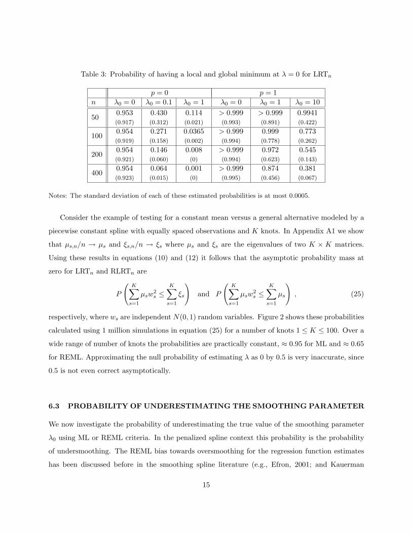
Table 3: Probability of having a local and global minimum at λ = 0 for LRTn

p = 0 p = 1n λ0 = 0 λ0 = 0.1 λ0 = 1 λ0 = 0 λ0 = 1 λ0 = 10

500.953(0.917)

0.430(0.312)

0.114(0.021)

> 0.999(0.993)

> 0.999(0.891)

0.9941(0.422)

1000.954(0.919)

0.271(0.158)

0.0365(0.002)

> 0.999(0.994)

0.999(0.778)

0.773(0.262)

2000.954(0.921)

0.146(0.060)

0.008(0)

> 0.999(0.994)

0.972(0.623)

0.545(0.143)

4000.954(0.923)

0.064(0.015)

0.001(0)

> 0.999(0.995)

0.874(0.456)

0.381(0.067)

Notes: The standard deviation of each of these estimated probabilities is at most 0.0005.

Consider the example of testing for a constant mean versus a general alternative modeled by a

piecewise constant spline with equally spaced observations and K knots. In Appendix A1 we show

that µs,n/n → µs and ξs,n/n → ξs where µs and ξs are the eigenvalues of two K × K matrices.

Using these results in equations (10) and (12) it follows that the asymptotic probability mass at

zero for LRTn and RLRTn are

P

(K∑

s=1

µsw2s ≤

K∑

s=1

ξs

)and P

(K∑

s=1

µsw2s ≤

K∑

s=1

µs

), (25)

respectively, where ws are independent N(0, 1) random variables. Figure 2 shows these probabilities

calculated using 1 million simulations in equation (25) for a number of knots 1 ≤ K ≤ 100. Over a

wide range of number of knots the probabilities are practically constant, ≈ 0.95 for ML and ≈ 0.65

for REML. Approximating the null probability of estimating λ as 0 by 0.5 is very inaccurate, since

0.5 is not even correct asymptotically.

6.3 PROBABILITY OF UNDERESTIMATING THE SMOOTHING PARAMETER

We now investigate the probability of underestimating the true value of the smoothing parameter

λ0 using ML or REML criteria. In the penalized spline context this probability is the probability

of undersmoothing. The REML bias towards oversmoothing for the regression function estimates

has been discussed before in the smoothing spline literature (e.g., Efron, 2001; and Kauerman

15

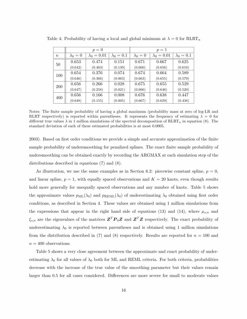
Table 4: Probability of having a local and global minimum at λ = 0 for RLRTn

p = 0 p = 1n λ0 = 0 λ0 = 0.01 λ0 = 0.1 λ0 = 0 λ0 = 0.01 λ0 = 0.1

500.653(0.642)

0.474(0.463)

0.151(0.139)

0.671(0.660)

0.667(0.656)

0.625(0.616)

1000.654(0.646)

0.376(0.366)

0.074(0.063)

0.674(0.663)

0.664(0.655)

0.589(0.579)

2000.656(0.647)

0.266(0.258)

0.028(0.021)

0.675(0.666)

0.655(0.646)

0.529(0.520)

4000.656(0.648)

0.166(0.155)

0.008(0.005)

0.676(0.667)

0.638(0.629)

0.447(0.438)

Notes: The finite sample probability of having a global maximum (probability mass at zero of log-LR andRLRT respectively) is reported within parentheses. It represents the frequency of estimating λ = 0 fordifferent true values λ in 1 million simulations of the spectral decomposition of RLRTn in equation (8). Thestandard deviation of each of these estimated probabilities is at most 0.0005.

2003). Based on first order conditions we provide a simple and accurate approximation of the finite

sample probability of undersmoothing for penalized splines. The exact finite sample probability of

undersmoothing can be obtained exactly by recording the ARGMAX at each simulation step of the

distributions described in equations (7) and (8).

As illustration, we use the same examples as in Section 6.2: piecewise constant spline, p = 0,

and linear spline, p = 1, with equally spaced observations and K = 20 knots, even though results

hold more generally for unequally spaced observations and any number of knots. Table 5 shows

the approximate values pML(λ0) and pREML(λ0) of underestimating λ0 obtained using first order

conditions, as described in Section 4. These values are obtained using 1 million simulations from

the expressions that appear in the right hand side of equations (13) and (14), where µs,n and

ξs,n are the eigenvalues of the matrices ZT P 0Z and ZT Z respectively. The exact probability of

underestimating λ0 is reported between parentheses and is obtained using 1 million simulations

from the distribution described in (7) and (8) respectively. Results are reported for n = 100 and

n = 400 observations.

Table 5 shows a very close agreement between the approximate and exact probability of under-

estimating λ0 for all values of λ0 both for ML and REML criteria. For both criteria, probabilities

decrease with the increase of the true value of the smoothing parameter but their values remain

larger than 0.5 for all cases considered. Differences are more severe for small to moderate values

16

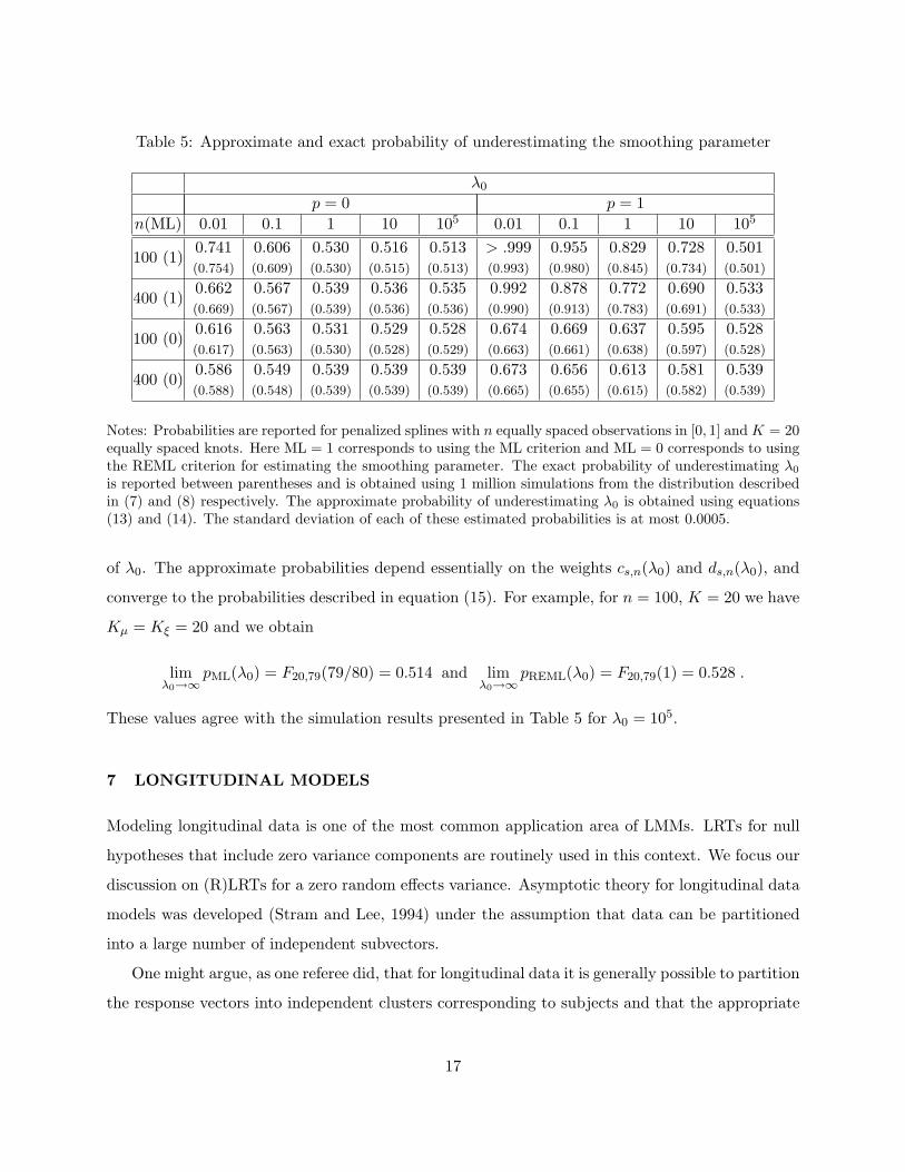
Table 5: Approximate and exact probability of underestimating the smoothing parameter

λ0

p = 0 p = 1n(ML) 0.01 0.1 1 10 105 0.01 0.1 1 10 105

100 (1)0.741(0.754)

0.606(0.609)

0.530(0.530)

0.516(0.515)

0.513(0.513)

> .999(0.993)

0.955(0.980)

0.829(0.845)

0.728(0.734)

0.501(0.501)

400 (1)0.662(0.669)

0.567(0.567)

0.539(0.539)

0.536(0.536)

0.535(0.536)

0.992(0.990)

0.878(0.913)

0.772(0.783)

0.690(0.691)

0.533(0.533)

100 (0)0.616(0.617)

0.563(0.563)

0.531(0.530)

0.529(0.528)

0.528(0.529)

0.674(0.663)

0.669(0.661)

0.637(0.638)

0.595(0.597)

0.528(0.528)

400 (0)0.586(0.588)

0.549(0.548)

0.539(0.539)

0.539(0.539)

0.539(0.539)

0.673(0.665)

0.656(0.655)

0.613(0.615)

0.581(0.582)

0.539(0.539)

Notes: Probabilities are reported for penalized splines with n equally spaced observations in [0, 1] and K = 20equally spaced knots. Here ML = 1 corresponds to using the ML criterion and ML = 0 corresponds to usingthe REML criterion for estimating the smoothing parameter. The exact probability of underestimating λ0

is reported between parentheses and is obtained using 1 million simulations from the distribution describedin (7) and (8) respectively. The approximate probability of underestimating λ0 is obtained using equations(13) and (14). The standard deviation of each of these estimated probabilities is at most 0.0005.

of λ0. The approximate probabilities depend essentially on the weights cs,n(λ0) and ds,n(λ0), and

converge to the probabilities described in equation (15). For example, for n = 100, K = 20 we have

Kµ = Kξ = 20 and we obtain

limλ0→∞

pML(λ0) = F20,79(79/80) = 0.514 and limλ0→∞

pREML(λ0) = F20,79(1) = 0.528 .

These values agree with the simulation results presented in Table 5 for λ0 = 105.

7 LONGITUDINAL MODELS

Modeling longitudinal data is one of the most common application area of LMMs. LRTs for null

hypotheses that include zero variance components are routinely used in this context. We focus our

discussion on (R)LRTs for a zero random effects variance. Asymptotic theory for longitudinal data

models was developed (Stram and Lee, 1994) under the assumption that data can be partitioned

into a large number of independent subvectors.

One might argue, as one referee did, that for longitudinal data it is generally possible to partition

the response vectors into independent clusters corresponding to subjects and that the appropriate

17

asymptotics is obtained by allowing the number of subjects to increase rather than the number of

observations per subject. However, in our view, this argument has several drawbacks.

The object of interest is the finite sample distribution of the test statistic. If this is available,

then it should be used. If an asymptotic distribution is used, then the type of asymptotics used

should be that which gives the best approximation to the finite-sample distribution. In Section 7.1,

for the random intercept longitudinal model, we show that if the number of subjects is less than

100 then the 50 : 50 mixture of chi squared distributions is a poor approximation of the (R)LRT

finite sample distribution, regardless of the number of observations per subject. For this example

we would use the finite sample distribution of the (R)LRT statistic, as derived by Crainiceanu and

Ruppert (2003).

Moreover, for many commonly used semiparametric models there are random effects in the

submodel for the population mean, so that the data cannot be divided into independent subvectors

and the results of Stram and Lee (1994) do not apply to this type of models.. For example, suppose

that n subjects in M groups are observed and their response curves are recorded over time. The

mean response of a subject can be decomposed as the corresponding group mean and the deviation

of the subject mean from the group mean. The group mean can farther be decomposed as the

overall mean and the deviation of the group mean from the overall mean. In Section 7.2 we show

that if the overall mean is modelled nonparametrically in this way, then the response vector cannot

be partitioned into more than one independent subvector. Moreover, if the overall mean is modelled

parametrically and the group deviations are modelled nonparametrically, then the response vector

cannot be partitioned into more than M independent subvectors, where M rarely exceeds 5 in

applications.

7.1 RANDOM INTERCEPT LONGITUDINAL MODEL

Consider the random intercept longitudinal model with K subjects and J(k) observations per

subject k

Ykj = β0 +S∑

s=1

βsx(s)kj + bk + εkj , k = 1, . . . ,K and j = 1, . . . , J(k) . (26)

where εkj are i.i.d. random variables N(0, σ2ε ), bk are i.i.d. intercepts distributed N(0, σ2

b ) indepen-

dent of εkj and denote by λ = σ2b/σ2

ε . In model (26) β0 and βs, s = 1, . . . , S are fixed unknown

parameters and x(s)kj is the j-th observation for the k-th subject on the s-th covariate.

18

The matrix X for fixed effects is a JK × (S + 1) matrix with the first column containing

only 1’s and the last S containing the corresponding values of x’s. The matrix Z is a JK × K

matrix with every column containing only zeros with the exception of a J-dimensional vector of

1’s corresponding to the random intercept for each subject. For this model Σ = IK , p = S + 1 and

n =∑K

k=1 J(k).

The eigenvalues of the matrices ZT P 0Z and ZT Z can be computed numerically and the finite

sample distributions of (R)LRTn statistics can be simulated using results in section 2. In particular,

properties such as probability mass at zero and probability of underestimating the true value of λ0

can be obtained in seconds.

In some cases these eigenvalues can be calculated explicitly. Consider the case of equal number

of observations per subject, J(k) = J for k = 1, . . . , K, one covariate, S = 1, and x(1)kj = xkj = j.

This example is routinely found in practice when K subjects are observed at equally spaced intervals

in time and time itself is used as a covariate. It is easy to show that for this example µs,n = J for

s = 1, . . . , K − 1, µK,n = 0 and ξs,n = J for s = 1, . . . , K. These eigenvalues are identical to the

corresponding eigenvalues for the balanced one-way ANOVA model and all distributional results

discussed in section 5 apply to this example.

If the covariates are not equally spaced and/or there are unequal numbers of observations per

subject then the eigenvalues of ZT P 0Z cannot be computed explicitly. In particular, the F distri-

bution cannot be used to compute the probability mass at zero or the probability of underestimating

the true signal to noise ratio, but our methodology could be.

7.2 NONPARAMETRIC LONGITUDINAL MODELS

Nested families of curves in longitudinal data analysis can be modeled nonparametrically using

penalized splines. An important advantage of low order smoothers, such as penalized splines, is the

reduction in the dimensionality of the problem. Moreover, smoothing can be done using standard

mixed model software because splines can be viewed as BLUPs in mixed models.

In this context, likelihood and restricted likelihood ratio statistics could be used to test for

effects of interest. For example, the hypothesis that a curve is linear is equivalent to a zero vari-

ance component being zero. While computing the test statistics is straightforward using standard

software, the null distribution theory is complex. Modified asymptotic theory for testing whether

a parameter is on the boundary of the parameter space does not apply because data are correlated

19

under the alternative (usually the full model).

Brumback and Rice (1998) study an important class of models for longitudinal data. In this

paper, we consider a subclass of those models. In particular, we assume that repeated observations

are taken on each of n subjects divided into M groups. Suppose that yij is the j-th observation on

the i-th subject recorded at time tij , where 1 ≤ i ≤ I, 1 ≤ j ≤ J(i), and n =∑I

i=1 J(i) is the total

number of observations. Consider the nonparametric model

yij = f(tij) + fg(i)(tij) + fi(tij) + εij , (27)

where εij are independent N(0, σ2ε ) errors and g(i) denotes the group corresponding to the i-th

subject. The population curve f(·), the deviations of the g(i) group from the population curve,

fg(i)(tij), and the deviation of the ith subject’s curve from the population average, fi(·), are modeled

nonparametrically. Models similar to (27) have been studied by many other authors, e.g., Wang

(1998).

We model the population, group and subject curves as penalized splines with a relatively small

number of knots

f(t) =∑p

s=0 βsts +

∑K1k=1 bk(t− κ1,k)

p+

fg(t) =∑p

s=0 βgsts +

∑K2k=1 ugk(t− κ2,k)

p+

fi(t) =∑p

s=0 aists +

∑K3k=1 vik(t− κ3,k)

p+ .

For the population curve β0, . . . , βp will be treated as fixed effects and b1, . . . , bK will be treated as

independent random coefficients distributed N(0, σ2b ). In LMM’s, usually parameters are treated

as random effects because they are subject-specific and the subjects have been sampled randomly.

Here, b1, . . . , bK are treated as random effects for an entirely different reason. Modeling them as

random specifies a Bayesian prior and allows for shrinkage that assures smoothness of the fit.

For the group curves βgs, g = 1, . . . ,M , s = 1, . . . , p, will be treated as fixed effects and ugk,

k = 1, . . . ,K, will be treated as random coefficients distributed N(0, σ2g). To make the model

identifiable we impose restrictions on βgs

M∑

g=1

βgs = 0 or βMs = 0 for s = 1, . . . , p .

This model assumes that the groups are fixed, e.g., are determined by fixed treatments. If the

groups were chosen randomly, then the model would be changed somewhat. The parameters βgs,

20

g = 1, . . . , M , s = 1, . . . , p, would be treated as random effects and the σ2g might be assumed to be

equal or to be i.i.d. from some distribution such as an inverse gamma.

For the subject curves, ais, 1 ≤ i ≤ n, will be treated as independent random coefficients

distributed N(0, σ2a,s), which is a typical random effects assumption since the subjects are sampled

randomly. Moreover vik will be treated as independent random coefficients distributed N(0, σ2v).

With the additional assumption that bk, aik, vik and εij are independent, the nonparametric model

(27) can be rewritten as a LMM with p + M + 3 variance components

Y = X�β + XGβG + Zbb + ZGuG + Zaa + Zvv + ε , (28)

where β = (β0, . . . , βp)T , βg = (βg0, . . . , βgp)T , βG = (βT1 , . . . ,βT

M ), ug = (ug1, . . . , ugK2)T , uG =

(uT1 , . . . , uT

M )T , as = (a1s, . . . , ans)T , a = (aT0 , . . . ,aT

p )T and v = (v11, . . . , vnK3). The X and Z

matrices are defined accordingly.

By inspecting the form (28) of model (27), some interesting features of the model are revealed.

If σ2b > 0 then the vector Y cannot be partitioned into more than one independent subvectors due

to the term Zb. If σ2b = 0 but at least one of σ2

g > 0 then Y cannot be partitioned into more

than M independent subvectors due to the term ZGuG. In other words, if the overall or one of

the group means are modeled nonparametrically then the assumptions for obtaining the Self and

Liang type of results fail to hold.

When longitudinal data are modeled semiparametrically in this way and there is more than

one variance component, deriving the finite sample distribution of (R)LRT for testing that certain

variance components are zero is not straightforward. The distribution of the LRT and RLRT

statistics will depend on those variance components, if any, that are not completely specified by

the null hypothesis. Therefore, exact tests are generally not possible. We recommend that the

parametric bootstrap be used to approximate the finite sample distributions of the test statistics.

However, the bootstrap will be much more computationally intensive that the simulations we have

been able to develop.

8 DISCUSSION

We considered estimation of the ratio between the random effects and error variances in a LMM with

one variance component and we examined the probability mass at zero of the (RE)ML estimator, as

well as the probability of underestimating the true parameter λ0. We provided simple formulae for

21

calculating the approximations of these probabilities based on first order conditions and show that

these approximations are very good at least for balanced one-way ANOVA and penalized spline

models.

One important application of our results is to provide exact finite sample and asymptotic

probability mass at zero of the (R)LRTn when testing that the random effects variance is zero

in a LMM with one variance component. Our results explain why asymptotic theory, such as

derived by Self and Liang, should be used cautiously. In particular, even in the simplest example

of balanced one-way ANOVA model, which satisfies the Self and Liang independence assumptions,

the 0.5 : 0.5 mixture approximation holds only when the number of levels goes to infinity but fails

when the number of levels is moderate (< 100), regardless of the number of observations per level.

For penalized spline models the 0.5 : 0.5 mixture approximation does not hold regardless of the

number of knots K and number of observations n. As we mentioned in the introduction, another

model where the Self and Liang theory does not apply is the regression with a stochastic trend

analyzed by Shephard and Harvey (1990) and Shephard (1993). In contrast, the exact finite sample

distribution of (R)LRTn can be easily obtained as described by Crainiceanu and Ruppert (2003).

We also derived the probability of underestimating the true ratio of random effects and error

variances λ0 using ML and REML criteria. We showed that using first order conditions provides an

excellent approximation of the exact probability. Both for one-way ANOVA and penalized spline

models this probability is larger than 0.5 showing that (RE)ML underestimates more often than

overestimates the true parameter.

Acknowledgement

We thank the Associate Editor and two referees for their helpful comments.

REFERENCES

Brumback, B., and Rice, J.A. (1998), “Smoothing spline models for the analysis of nested and

crossed samples of curves (with discussion),” Journal of the American Statistical Association,

93, 961–994.

Brumback, B., Ruppert, D., and Wand, M. P. (1999), “Comment on ‘Variable selection and

function estimation in additive nonparametric regression using data-based prior’ ” by Shively,

22

Kohn, and Wood, Journal of the American Statistical Association, 94, 794–797.

Crainiceanu, C. M., Ruppert, D. (2003), “Likelihood ratio tests in linear mixed models with one

variance component,” Journal of Royal Statistical Society - Series B, to appear.

Crainiceanu, C. M., Ruppert, D., and Claeskens, G., Wand, M. P. (2003), “Exact Likelihood Ratio

Tests for Penalized Splines,” under revision, available at www.orie.cornell.edu/~davidr/papers.

Das, R., and Sinha, B. K. (1987), “Robust optimum invariant unbiased tests for variance com-

ponents,” In Proceedings of the Second International Tampere Conference in Statistics, T.

Pukkila and S. Puntanen, ed., University of Tampere, Finland, pp. 317–342.

Davies, R. B. (1980), “The distribution of a linear combination of χ2 random variables,” Applied

Statistics, 29, 323–333.

Efron, B. (2001), “Selection criteria for scatterplot smoothers,” The Annals of Statistics, 29,

470–504.

Farebrother, R. W. (1990), “The distribution of a quadratic form in normal variables,” Applied

Statistics, 39, 294–309.

Gray, R. J. (1994), “Spline-Based Tests in Survival Analysis,” Biometrics, 50, 640–652.

Harville, D. A. (1974), “Bayesian inference for variance components using only error contrasts,”

Biometrika, 61, 383–385.

Harville, D. A. (1977), “Maximum likelihood approaches to variance component estimation and

to related problems,” Journal of the American Statistical Association, 72, 320–338.

Hoffman, K., Kunze, R. (1971), Linear Algebra, Prentice-Hall, Englewood Cliffs, New Jersey.

Kauerman, G. (2003), “A note on bandwidth selection for penalised spline smoothing,” manuscript.

Khuri, A. I. (1994), “The probability of a negative linear combination of independent mean

squares,” Biometrical Journal, 36, 899–910.

Khuri, A. I., Mathew, T., Sinha, B. K. (1998), Statistical Tests for Mixed Linear Models, Wiley,

New York.

Patterson, H. D., and Thompson, R. (1971), “Recovery of inter-block information when block

sizes are unequal,” Biometrika, 58, 545–554.

23

Pinheiro, J. C., Bates, D.M. (2000), Mixed-Effects Models in S and S-Plus, Springer-Verlag, New

York.

Ruppert, D. (2002), “Selecting the number of knots for penalized splines,” Journal of Computa-

tional and Graphical Statistics, 11, 205–224.

Ruppert, D., Wand, M. P., and Carroll, R. J. (2003) Semiparametric Regression, Cambridge

University Press, Cambridge.

Searle, S. R., Casella, G., McCulloch, C. E. (1992), Variance components, Wiley, New York.

Self, S. G., and Liang, K. Y. (1987), “Asymptotic properties of maximum likelihood estimators

and likelihood ratio tests under non-standard conditions,” Journal of the American Statistical

Association, 82, 605-610.

Self, S. G., and Liang, K. Y. (1995), “On the Asymptotic Behaviour of the Pseudolikelihood Ratio

Test Statistic,” Journal of Royal Statistical Society B, 58, 785-796.

Shephard, N. G., Harvey, A. C. (1990), “On the probability of estimating a deterministic compo-

nent in the local level model,” Journal of Time Series Analysis, 4, 339-347.

Shephard, N. G. (1993), “Maximum Likelihood Estimation of Regression Models with Stochastic

Trend Components,” Journal of the American Statistical Association, 88, 590-595.

Stram, D. O., Lee, J. W. (1994), “Variance Components Testing in the Longitudinal Mixed Effects

Model,” Biometrics, 50, 1171-1177.

Wahba, G. (1978), “Improper priors, spline smoothing, and the problem of guarding against model

errors in regression,” Journal of Royal Statistical Society B, 40, 364–372.

Wahba, G. (1990), Spline Models for Observational Data, SIAM, Philadelphia.

Yu, H., Searle, S. R., and McCulloch, C. E. (1994), “Properties of maximum likelihood estimators

of variance components in the one-way classification model, balanced data,” Communications

in Statistics - Simulation and Computation, 23, 897-914.

Appendix A1

Consider the case of a piecewise constant spline with K knots

yi = β0 +K∑

k=1

bkI(xi > κk) + εi ,

24

where I(·) is the indicator function. Denote by nk(n) the number of covariate observations larger

than the k-th knot and assume that limn→∞ nk(n)/n = uk. In the case of equally spaced observa-

tions in [0, 1] this assumption holds and uk = 1− k/(K + 1). The (i, k)-th element of the Z matrix

is I(xi > κk) showing the (l, k)-th element of ZT Z matrix is

ul,k(n) =n∑

i=1

I(xi > κl)I(xi > κk) = nmax(l,k)(n) .

Therefore ul,k(n)/n → umax(l,k) or, if we denote by U the K × K matrix with umax(l,k) as the

(l, k)-th entry,

limn→∞

ZT Z

n= U .

Similarly we obtain that

limn→∞

ZT P 0Z

n= V ,

where the (l, k)-th entry of the matrix V is vl,k = umax(l,k) − uluk. If we denote by µs and ξs the

eigenvalues of V and U matrices it follows that

limn→∞µs,n/n = µs and lim

n→∞ ξs,n/n = ξs .

25

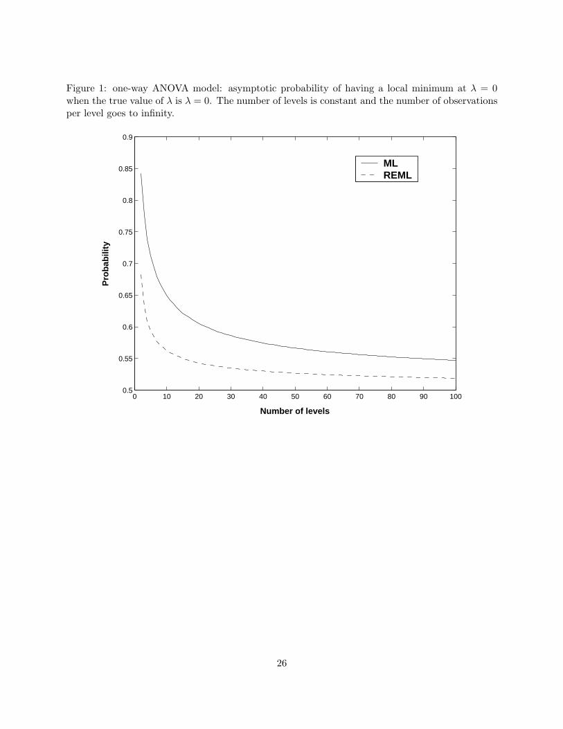
Figure 1: one-way ANOVA model: asymptotic probability of having a local minimum at λ = 0when the true value of λ is λ = 0. The number of levels is constant and the number of observationsper level goes to infinity.

0 10 20 30 40 50 60 70 80 90 1000.5

0.55

0.6

0.65

0.7

0.75

0.8

0.85

0.9

Number of levels

Pro

bab

ility

MLREML

26

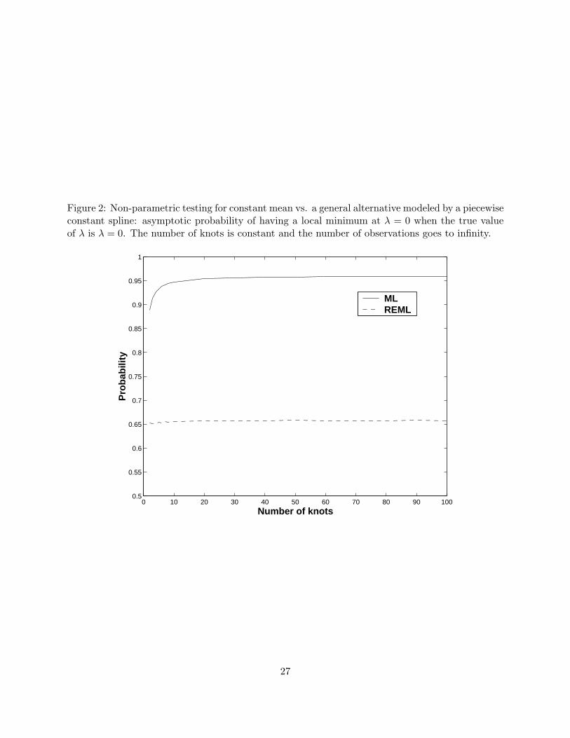
Figure 2: Non-parametric testing for constant mean vs. a general alternative modeled by a piecewiseconstant spline: asymptotic probability of having a local minimum at λ = 0 when the true valueof λ is λ = 0. The number of knots is constant and the number of observations goes to infinity.

0 10 20 30 40 50 60 70 80 90 1000.5

0.55

0.6

0.65

0.7

0.75

0.8

0.85

0.9

0.95

1

Number of knots

Pro

bab

ility

MLREML

27