Chapter 4 E cient Likelihood Estimation and Related Tests · Chapter 4 E cient Likelihood...
42
1 Chapter 4 Efficient Likelihood Estimation and Related Tests 1. Maximum likelihood and efficient likelihood estimation 2. Likelihood ratio, Wald, and Rao (or score) tests 3. Examples 4. Consistency of Maximum Likelihood Estimates 5. The EM algorithm and related methods 6. Nonparametric MLE 7. Limit theory for the statistical agnostic: P/ ∈P
Transcript of Chapter 4 E cient Likelihood Estimation and Related Tests · Chapter 4 E cient Likelihood...

1
Chapter 4Efficient Likelihood Estimation
and Related Tests
1. Maximum likelihood and efficient likelihood estimation
2. Likelihood ratio, Wald, and Rao (or score) tests
3. Examples
4. Consistency of Maximum Likelihood Estimates
5. The EM algorithm and related methods
6. Nonparametric MLE
7. Limit theory for the statistical agnostic: P /∈ P

2
Chapter 4
Efficient Likelihood Estimation andRelated Tests
1 Maximum likelihood and efficient likelihood estimation
We begin with a brief discussion of Kullback - Leibler information.
Definition 1.1 Let P be a probability measure, and let Q be a sub-probability measure on (X,A)with densities p and q with respect to a sigma-finite measure µ (µ = P + Q always works). ThusP (X) = 1 and Q(X) ≤ 1. Then the Kullback - Leibler information K(P,Q) is
K(P,Q) ≡ EP{
logp(X)
q(X)
}.(1)
Lemma 1.1 For a probability measure P and a (sub-)probability measure Q, the Kullback-Leiblerinformation K(P,Q) is always well-defined, and
K(P,Q)
{∈ [0,∞] always= 0 if and only if Q = P .
Proof. Now
K(P,Q) =
{log 1 = 0 if P = Q ,logM > 0 if P = MQ, M > 1 .
If P 6= MQ, then Jensen’s inequality is strict and yields
K(P,Q) = EP
(− log
q(X)
p(X)
)> − logEP
(q(X)
p(X)
)= − logEQ1[p(X)>0]
≥ − log 1 = 0 .
2
Now we need some assumptions and notation. Suppose that the model P is given by
P = {Pθ : θ ∈ Θ} .
3
4 CHAPTER 4. EFFICIENT LIKELIHOOD ESTIMATION AND RELATED TESTS
We will impose the following hypotheses about P:
Assumptions:
A0. θ 6= θ∗ implies Pθ 6= Pθ∗ .
A1. A ≡ {x : pθ(x) > 0} does not depend on θ.
A2. Pθ has density pθ with respect to the σ−finite measure µ and X1, . . . , Xn are i.i.d. Pθ0 ≡ P0.
Notation:
L(θ) ≡ Ln(θ) ≡ L(θ|X) ≡n∏i=1
pθ(Xi) ,
l(θ) = l(θ|X) ≡ ln(θ) ≡ logLn(θ) =
n∑i=1
log pθ(Xi) ,
l(B) ≡ l(B|X) ≡ ln(B) = supθ∈B
l(θ|X) .
Here is a preliminary result which motivates our definition of the maximum likelihood estimator.
Theorem 1.1 If A0 - A2 hold, then for θ 6= θ0
1
nlog
(Ln(θ0)
Ln(θ)
)=
1
n
n∑i=1
logpθ0(Xi)
pθ(Xi)→a.s. K(Pθ0 , Pθ) > 0 ,
and hence
Pθ0(Ln(θ0|X) > Ln(θ|X))→ 1 as n→∞ .
Proof. The first assertion is just the strong law of large numbers; note that
Eθ0 logpθ0(X)
pθ(X)= K(Pθ0 , Pθ) > 0
by lemma 1.1 and A0. The second assertion is an immediate consequence of the first. 2
Theorem 1.1 motivates the following definition.
Definition 1.2 The value θ = θn of θ which maximizes the likelihood L(θ|X), if it exists and isunique, is the maximum likelihood estimator (MLE) of θ. Thus L(θ) = L(Θ) or l(θn) = l(Θ).
Cautions:
• θn may not exist.
• θn may exist, but may not be unique.
• Note that the definition depends on the version of the density pθ which is selected; since thisis not unique, different versions of pθ lead to different MLE’s
1. MAXIMUM LIKELIHOOD AND EFFICIENT LIKELIHOOD ESTIMATION 5
When Θ ⊂ Rd, the usual approach to finding θn is to solve the likelihood (or score) equations
l(θ|X) ≡ ln(θ) = 0 ;(2)
i.e. lθi(θ|X) = 0, i = 1, . . . , d. The solution θn say, may not be the MLE, but may yield simply alocal maximum of l(θ).
The likelihood ratio statistic for testing H : θ = θ0 versus K : θ 6= θ0 is
λn =L(Θ)
L(θ0)=
supθ∈Θ L(θ|X)
L(θ0|X)=L(θn)
L(θ0),
λn =L(θn)
L(θ0).
Write P0, E0 for Pθ0 , Eθ0 . Here are some more assumptions about the model P which we will useto treat these estimators and test statistics.
Assumptions, continued:
A3. Θ contains an open neighborhood Θ0 ⊂ Rd of θ0 for which:
(i) For µ a.e. x, l(θ|x) ≡ log pθ(x) is twice continuously differentiable in θ.
(ii) For a.e. x, the third order derivatives exist and···l jkl (θ|x) satisfy |
···l jkl (θ|x)| ≤Mjkl(x)
for θ ∈ Θ0 for all 1 ≤ j, k, l ≤ d with E0Mjkl(X) <∞.
A4. (i) E0{lj(θ0|X)} = 0 for j = 1, . . . , d.
(ii) E0{l2j (θ0|X)} <∞ for j = 1, . . . , d.
(iii) I(θ0) = (−E0{ljk(θ0|X)}) is positive definite.
Let
Zn ≡1√n
n∑i=1
l(θ0|Xi) and l(θ0|X) = I−1(θ0)l(θ0|X) ,
so that
I−1(θ0)Zn =1√n
n∑i=1
l(θ0|Xi) .
Theorem 1.2 Suppose that X1, . . . , Xn are i.i.d. Pθ0 ∈ P with density pθ0 where P satisfies A0 -A4. Then:
(i) With probability converging to 1 there exist solutions θn of the likelihood equations such thatθn →p θ0 when P0 = Pθ0 is true.
(ii) θn is asymptotically linear with influence function l(θ0|x). That is,
√n(θn − θ0) = I−1(θ0)Zn + op(1) =
1√n
n∑i=1
l(θ0|Xi) + op(1)
→d I−1(θ0)Z ≡ D ∼ Nd(0, I−1(θ0)) .
6 CHAPTER 4. EFFICIENT LIKELIHOOD ESTIMATION AND RELATED TESTS
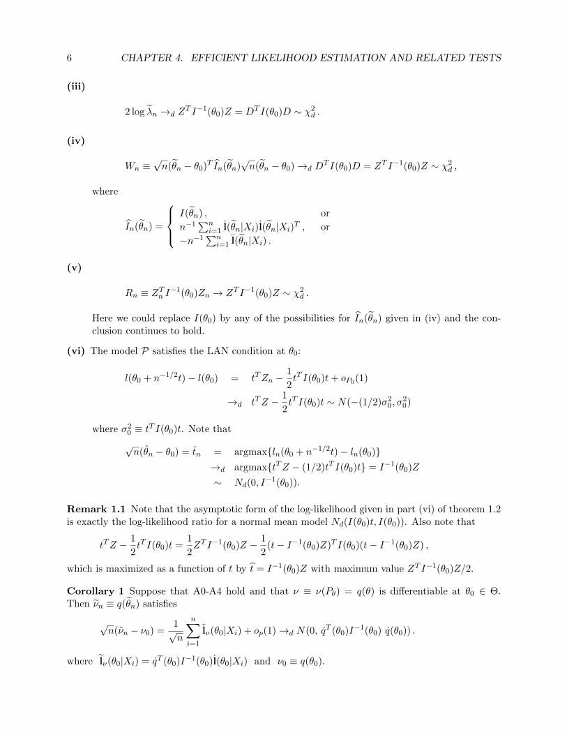
(iii)
2 log λn →d ZT I−1(θ0)Z = DT I(θ0)D ∼ χ2
d .
(iv)
Wn ≡√n(θn − θ0)T In(θn)
√n(θn − θ0)→d D
T I(θ0)D = ZT I−1(θ0)Z ∼ χ2d ,
where
In(θn) =
I(θn) , or
n−1∑n
i=1 l(θn|Xi)l(θn|Xi)T , or
−n−1∑n
i=1 l(θn|Xi) .
(v)
Rn ≡ ZTn I−1(θ0)Zn → ZT I−1(θ0)Z ∼ χ2d .
Here we could replace I(θ0) by any of the possibilities for In(θn) given in (iv) and the con-clusion continues to hold.
(vi) The model P satisfies the LAN condition at θ0:
l(θ0 + n−1/2t)− l(θ0) = tTZn −1
2tT I(θ0)t+ oP0(1)
→d tTZ − 1
2tT I(θ0)t ∼ N(−(1/2)σ2
0, σ20)
where σ20 ≡ tT I(θ0)t. Note that
√n(θn − θ0) = tn = argmax{ln(θ0 + n−1/2t)− ln(θ0)}
→d argmax{tTZ − (1/2)tT I(θ0)t} = I−1(θ0)Z
∼ Nd(0, I−1(θ0)).
Remark 1.1 Note that the asymptotic form of the log-likelihood given in part (vi) of theorem 1.2is exactly the log-likelihood ratio for a normal mean model Nd(I(θ0)t, I(θ0)). Also note that
tTZ − 1
2tT I(θ0)t =
1
2ZT I−1(θ0)Z − 1
2(t− I−1(θ0)Z)T I(θ0)(t− I−1(θ0)Z) ,
which is maximized as a function of t by t = I−1(θ0)Z with maximum value ZT I−1(θ0)Z/2.
Corollary 1 Suppose that A0-A4 hold and that ν ≡ ν(Pθ) = q(θ) is differentiable at θ0 ∈ Θ.Then νn ≡ q(θn) satisfies
√n(νn − ν0) =
1√n
n∑i=1
lν(θ0|Xi) + op(1)→d N(0, qT (θ0)I−1(θ0) q(θ0)) .
where lν(θ0|Xi) = qT (θ0)I−1(θ0)l(θ0|Xi) and ν0 ≡ q(θ0).
1. MAXIMUM LIKELIHOOD AND EFFICIENT LIKELIHOOD ESTIMATION 7
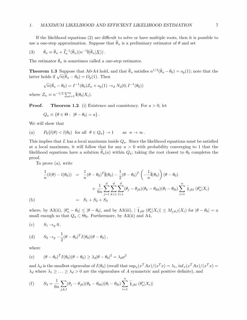
If the likelihood equations (2) are difficult to solve or have multiple roots, then it is possible touse a one-step approximation. Suppose that θn is a preliminary estimator of θ and set
θn ≡ θn + I−1n (θn)(n−1l(θn|X)) .(3)
The estimator θn is sometimes called a one-step estimator.
Theorem 1.3 Suppose that A0-A4 hold, and that θn satisfies n1/4(θn− θ0) = op(1); note that thelatter holds if
√n(θn − θ0) = Op(1). Then
√n(θn − θ0) = I−1(θ0)Zn + op(1)→d Nd(0, I
−1(θ0))
where Zn ≡ n−1/2∑n
i=1 l(θ0|Xi).
Proof. Theorem 1.2. (i) Existence and consistency. For a > 0, let
Qa ≡ {θ ∈ Θ : |θ − θ0| = a} .
We will show that
P0{l(θ) < l(θ0) for all θ ∈ Qa} → 1 as n→∞ .(a)
This implies that L has a local maximum inside Qa. Since the likelihood equations must be satisfiedat a local maximum, it will follow that for any a > 0 with probability converging to 1 that thelikelihood equations have a solution θn(a) within Qa; taking the root closest to θ0 completes theproof.
To prove (a), write
1
n(l(θ)− l(θ0)) =
1
n(θ − θ0)T l(θ0)− 1
2(θ − θ0)T
(− 1
nl(θ0)
)(θ − θ0)
+1
6n
d∑j=1
d∑k=1
d∑l=1
(θj − θj0)(θk − θk0)(θl − θl0)
n∑i=1
···l jkl (θ∗n|Xi)
= S1 + S2 + S3(b)
where, by A3(ii), |θ∗n − θ0| ≤ |θ − θ0|, and by A3(iii), |···l jkl (θ∗n|Xi)| ≤ Mj,k,l(Xi) for |θ − θ0| = a
small enough so that Qa ⊂ Θ0. Furthermore, by A3(ii) and A4,
S1 →p 0 ,(c)
S2 →p −1
2(θ − θ0)T I(θ0)(θ − θ0) ,(d)
where
(θ − θ0)T I(θ0)(θ − θ0) ≥ λd|θ − θ0|2 = λda2(e)
and λd is the smallest eigenvalue of I(θ0) (recall that supx(xTAx)/(xTx) = λ1, infx(xTAx)/(xTx) =λd where λ1 ≥ . . . ≥ λd > 0 are the eigenvalues of A symmetric and positive definite), and
S3 =1
6n
∑j,k,l
(θj − θj0)(θk − θk0)(θl − θl0)n∑i=1
···l jkl (θ∗n|Xi)|(f)
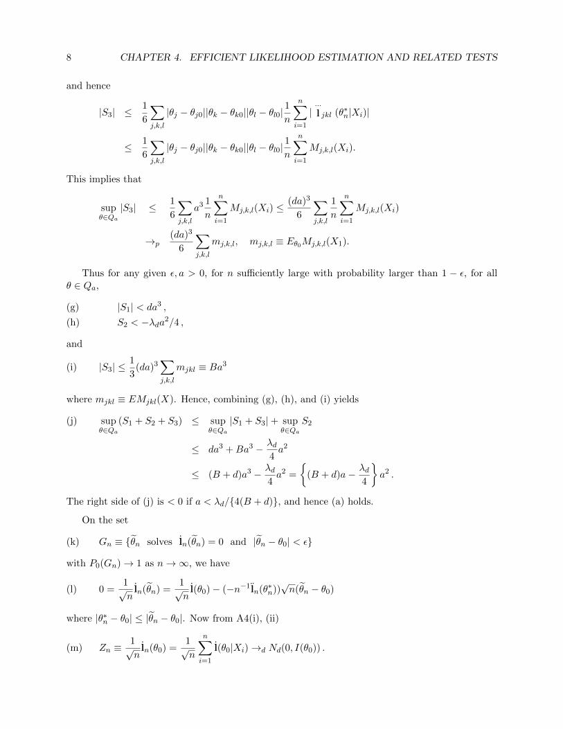
8 CHAPTER 4. EFFICIENT LIKELIHOOD ESTIMATION AND RELATED TESTS
and hence
|S3| ≤1
6
∑j,k,l
|θj − θj0||θk − θk0||θl − θl0|1
n
n∑i=1
|···l jkl (θ∗n|Xi)|
≤ 1
6
∑j,k,l
|θj − θj0||θk − θk0||θl − θl0|1
n
n∑i=1
Mj,k,l(Xi).
This implies that
supθ∈Qa
|S3| ≤ 1
6
∑j,k,l
a3 1
n
n∑i=1
Mj,k,l(Xi) ≤(da)3
6
∑j,k,l
1
n
n∑i=1
Mj,k,l(Xi)
→p(da)3
6
∑j,k,l
mj,k,l, mj,k,l ≡ Eθ0Mj,k,l(X1).
Thus for any given ε, a > 0, for n sufficiently large with probability larger than 1 − ε, for allθ ∈ Qa,
|S1| < da3 ,(g)
S2 < −λda2/4 ,(h)
and
|S3| ≤1
3(da)3
∑j,k,l
mjkl ≡ Ba3(i)
where mjkl ≡ EMjkl(X). Hence, combining (g), (h), and (i) yields
supθ∈Qa
(S1 + S2 + S3) ≤ supθ∈Qa
|S1 + S3|+ supθ∈Qa
S2(j)
≤ da3 +Ba3 − λd4a2
≤ (B + d)a3 − λd4a2 =
{(B + d)a− λd
4
}a2 .
The right side of (j) is < 0 if a < λd/{4(B + d)}, and hence (a) holds.
On the set
Gn ≡ {θn solves ln(θn) = 0 and |θn − θ0| < ε}(k)
with P0(Gn)→ 1 as n→∞, we have
0 =1√n
ln(θn) =1√n
l(θ0)− (−n−1ln(θ∗n))√n(θn − θ0)(l)
where |θ∗n − θ0| ≤ |θn − θ0|. Now from A4(i), (ii)
Zn ≡1√n
ln(θ0) =1√n
n∑i=1
l(θ0|Xi)→d Nd(0, I(θ0)) .(m)
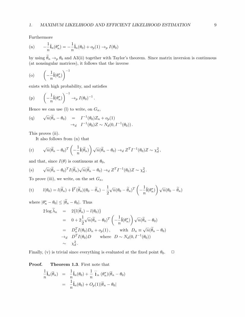
1. MAXIMUM LIKELIHOOD AND EFFICIENT LIKELIHOOD ESTIMATION 9
Furthermore
− 1
nln(θ∗n) = − 1
nln(θ0) + op(1)→p I(θ0)(n)
by using θn →p θ0 and A3(ii) together with Taylor’s theorem. Since matrix inversion is continuous(at nonsingular matrices), it follows that the inverse(
− 1
nl(θ∗n)
)−1
(o)
exists with high probability, and satisfies(− 1
nl(θ∗n)
)−1
→p I(θ0)−1 .(p)
Hence we can use (l) to write, on Gn,√n(θn − θ0) = I−1(θ0)Zn + op(1)(q)
→d I−1(θ0)Z ∼ Nd(0, I−1(θ0)) .
This proves (ii).It also follows from (n) that
√n(θn − θ0)T
(− 1
nl(θn)
)√n(θn − θ0)→d Z
T I−1(θ0)Z ∼ χ2d ,(r)
and that, since I(θ) is continuous at θ0,√n(θn − θ0)T I(θn)
√n(θn − θ0)→d Z
T I−1(θ0)Z ∼ χ2d .(s)
To prove (iii), we write, on the set Gn,
l(θ0) = l(θn) + lT (θn)(θ0 − θn)− 1
2
√n(θ0 − θn)T
(− 1
nl(θ∗n)
)√n(θ0 − θn)(t)
where |θ∗n − θ0| ≤ |θn − θ0|. Thus
2 log λn = 2{l(θn)− l(θ0)}
= 0 + 21
2
√n(θn − θ0)T
(− 1
nl(θ∗n)
)√n(θn − θ0)
= DTn I(θ0)Dn + op(1) , with Dn ≡
√n(θn − θ0)
→d DT I(θ0)D where D ∼ Nd(0, I−1(θ0))
∼ χ2d .
Finally, (v) is trivial since everything is evaluated at the fixed point θ0. 2
Proof. Theorem 1.3. First note that
1
nln(θn) =
1
nln(θ0) +
1
n
···l n (θ∗n)(θn − θ0)
=1
nln(θ0) +Op(1)|θn − θ0|
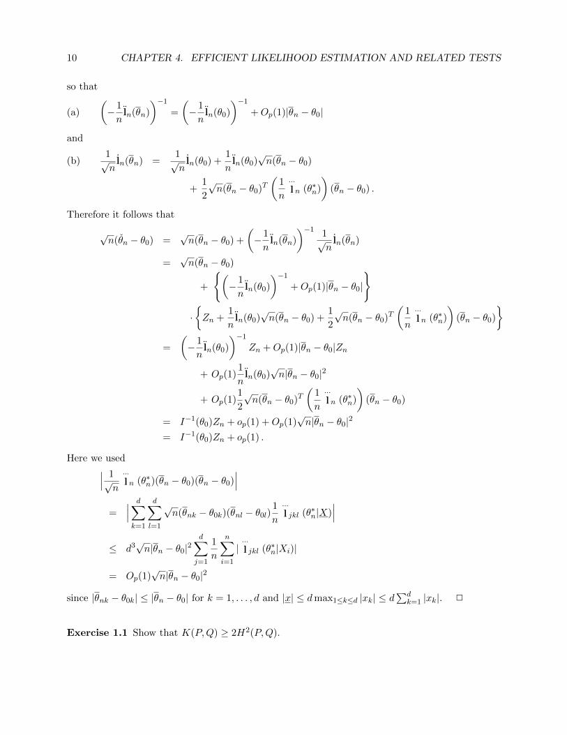
10 CHAPTER 4. EFFICIENT LIKELIHOOD ESTIMATION AND RELATED TESTS
so that(− 1
nln(θn)
)−1
=
(− 1
nln(θ0)
)−1
+Op(1)|θn − θ0|(a)
and
1√n
ln(θn) =1√n
ln(θ0) +1
nln(θ0)
√n(θn − θ0)(b)
+1
2
√n(θn − θ0)T
(1
n
···l n (θ∗n)
)(θn − θ0) .
Therefore it follows that
√n(θn − θ0) =
√n(θn − θ0) +
(− 1
nln(θn)
)−1 1√n
ln(θn)
=√n(θn − θ0)
+
{(− 1
nln(θ0)
)−1
+Op(1)|θn − θ0|
}
·{Zn +
1
nln(θ0)
√n(θn − θ0) +
1
2
√n(θn − θ0)T
(1
n
···l n (θ∗n)
)(θn − θ0)
}=
(− 1
nln(θ0)
)−1
Zn +Op(1)|θn − θ0|Zn
+ Op(1)1
nln(θ0)
√n|θn − θ0|2
+ Op(1)1
2
√n(θn − θ0)T
(1
n
···l n (θ∗n)
)(θn − θ0)
= I−1(θ0)Zn + op(1) +Op(1)√n|θn − θ0|2
= I−1(θ0)Zn + op(1) .
Here we used∣∣∣ 1√n
···l n (θ∗n)(θn − θ0)(θn − θ0)
∣∣∣=
∣∣∣ d∑k=1
d∑l=1
√n(θnk − θ0k)(θnl − θ0l)
1
n
···l jkl (θ∗n|X)
∣∣∣≤ d3√n|θn − θ0|2
d∑j=1
1
n
n∑i=1
|···l jkl (θ∗n|Xi)|
= Op(1)√n|θn − θ0|2
since |θnk − θ0k| ≤ |θn − θ0| for k = 1, . . . , d and |x| ≤ dmax1≤k≤d |xk| ≤ d∑d
k=1 |xk|. 2
Exercise 1.1 Show that K(P,Q) ≥ 2H2(P,Q).
2. THE WALD, LIKELIHOOD RATIO, AND SCORE (OR RAO) TESTS 11
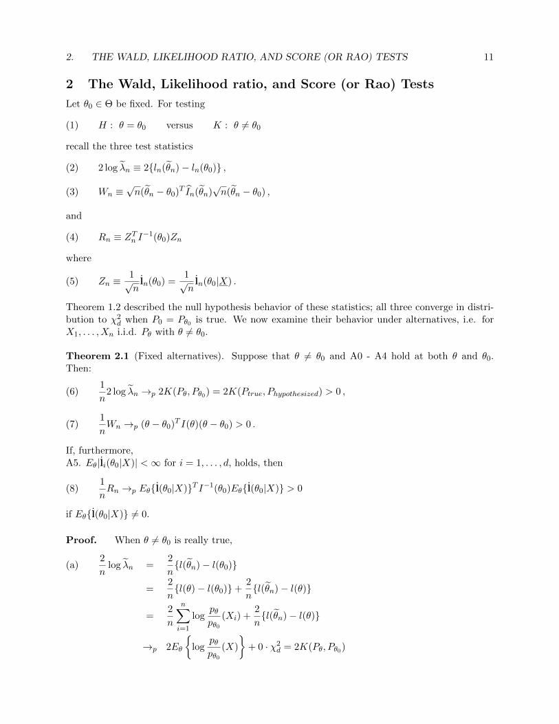
2 The Wald, Likelihood ratio, and Score (or Rao) Tests
Let θ0 ∈ Θ be fixed. For testing
H : θ = θ0 versus K : θ 6= θ0(1)
recall the three test statistics
2 log λn ≡ 2{ln(θn)− ln(θ0)} ,(2)
Wn ≡√n(θn − θ0)T In(θn)
√n(θn − θ0) ,(3)
and
Rn ≡ ZTn I−1(θ0)Zn(4)
where
Zn ≡1√n
ln(θ0) =1√n
ln(θ0|X) .(5)
Theorem 1.2 described the null hypothesis behavior of these statistics; all three converge in distri-bution to χ2
d when P0 = Pθ0 is true. We now examine their behavior under alternatives, i.e. forX1, . . . , Xn i.i.d. Pθ with θ 6= θ0.
Theorem 2.1 (Fixed alternatives). Suppose that θ 6= θ0 and A0 - A4 hold at both θ and θ0.Then:
1
n2 log λn →p 2K(Pθ, Pθ0) = 2K(Ptrue, Phypothesized) > 0 ,(6)
1
nWn →p (θ − θ0)T I(θ)(θ − θ0) > 0 .(7)
If, furthermore,A5. Eθ|li(θ0|X)| <∞ for i = 1, . . . , d, holds, then
1
nRn →p Eθ{l(θ0|X)}T I−1(θ0)Eθ{l(θ0|X)} > 0(8)
if Eθ{l(θ0|X)} 6= 0.
Proof. When θ 6= θ0 is really true,
2
nlog λn =
2
n{l(θn)− l(θ0)}(a)
=2
n{l(θ)− l(θ0)}+
2
n{l(θn)− l(θ)}
=2
n
n∑i=1
logpθpθ0
(Xi) +2
n{l(θn)− l(θ)}
→p 2Eθ
{log
pθpθ0
(X)
}+ 0 · χ2
d = 2K(Pθ, Pθ0)

12 CHAPTER 4. EFFICIENT LIKELIHOOD ESTIMATION AND RELATED TESTS
by the WLLN and Theorem 1.2. Also, by the Mann-Wald (or continuous mapping) theorem,
1
nWn = (θn − θ0)T In(θn)(θn − θ0)→p (θ − θ0)T I(θ)(θ − θ0) ,(b)
and, since
1√nZn =
1
nln(θ0) =
1
n
n∑i=1
l(θ0|Xi)→p Eθ{l(θ0|X)} ,(c)
it follows that
1
nRn →p Eθ{l(θ0|X)}T I−1(θ0)Eθ{l(θ0|X)} .(d)
2
Corollary 1 (Consistency of the likelihood ratio, Wald, and score tests). If Assumptions A0-A5hold, then the tests are consistent: i.e. if θ 6= θ0, then
Pθ(LR test rejects H) = Pθ(2 log λn ≥ χ2d,α)→ 1 ,(9)
Pθ(Wald test rejects H) = Pθ(Wn ≥ χ2d,α)→ 1 ,(10)
Pθ(score test rejects H) = Pθ(Rn ≥ χ2d,α)→ 1 ,(11)
assuming that Eθ{l(θ0|X)} 6= 0.
It remains to examine the behavior these three tests under local alternatives, θn = θ0 + tn−1/2
with t 6= 0. We first examine Zn and θn under θ0 using Le Cam’s third lemma 3.3.4.
Theorem 2.2 Suppose that A0-A4 hold. Then, if θn = θ0 + tn−1/2 is true, then under Pθn√n(θn − θ0)→d D + t ∼ Nd(t, I
−1(θ0)) ;(12)
furthermore,
Zn(θ0) ≡ 1√n
l(θ0|X)→d Z + I(θ0)t ∼ Nd(I(θ0)t, I(θ0)) .(13)
Hence we also have under Pθn ,
√n(θn − θn) =
√n(θn − θ0)−
√n(θn − θ0)(14)
→d D + t− t = D ∼ Nd(0, I−1(θ0)) ;
i.e. θn is locally regular. Furthermore,
Zn(θn) = Zn(θ0)−(− 1
nln(θ∗n)
)√n(θn − θ0)(15)
→d Z + I(θ0)t− I(θ0)t = Z ∼ Nd(0, I(θ0)) .

2. THE WALD, LIKELIHOOD RATIO, AND SCORE (OR RAO) TESTS 13
Proof. From the proof of theorem 1.2 we know that θn is asymptotically linear under P0 = Pθ0 :
√n(θn − θ0) =
1√n
n∑i=1
lθ(θ0|Xi) + op(1)
where lθ(x) ≡ I−1(θ0)lθ(x). Furthermore, it follows from theorem 1.2 part (vi) that the log likeli-hood ratio is asymptotically linear:
logdPnθndPnθ0
= l(θn)− l(θ0) = tTZn −1
2tT I(θ0)t+ op(1) .
Let a ∈ Rd. Then with Tn ≡ aT√n(θn − θ0) it follows from the multivariate CLT that(
Tn
logdPnθndPnθ0
)=
(aT√n(θn − θ0)
logdPnθndPnθ0
)
=1√n
n∑i=1
(aT lθ(θ0|Xi)
tT lθ(θ0|Xi)
)+
(0
−σ2/2
)+ op(1)
→d N2
((0
−σ2/2
),
(aT I−1(θ0)a aT t
aT t σ2
)).
Thus the hypothesis of Le Cam’s third lemma 3.3.4 is satisfied with c = aT t, and we deduce that,under Pθn ,(
aT√n(θn − θ0)
logdPnθndPnθ0
)→d N2
((aT t
+σ2/2
),
(aT I−1(θ0)a aT t
aT t σ2
)).
In particular, under Pθn ,
aT√n(θn − θ0)→d N(aT t, aT I−1(θ0)a) ,
and by the Cramer - Wold device this implies that under Pθn√n(θn − θ0)→d Nd(t, I
−1(θ0)) .
This, in turn, implies that
√n(θn − θn)→d Nd(0, I
−1(θ0)) .
under Pθn . The proof of the second part is similar, but easier, by taking Tn ≡ aTZn(θ0) which isalready a linear statistic. 2
Corollary 1 If A0-A4 hold, then if θn = θ0 + tn−1/2, under Pθn :
2 log λn →d (D + t)T I(θ0)(D + t) ∼ χ2d(δ) ,(16)
Wn →d (D + t)T I(θ0)(D + t) ∼ χ2d(δ) ,(17)
Rn →d (Z + I(θ0)t)T I−1(θ0)(Z + I(θ0)t) = (D + t)T I(θ0)(D + t) ∼ χ2d(δ)(18)
where δ = tT I(θ0)t.
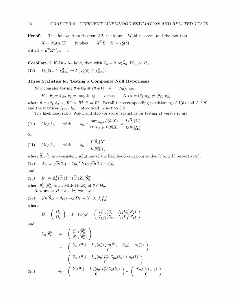
14 CHAPTER 4. EFFICIENT LIKELIHOOD ESTIMATION AND RELATED TESTS
Proof. This follows from theorem 2.2, the Mann - Wald theorem, and the fact that
X ∼ Nd(µ,Σ) implies XTΣ−1X ∼ χ2d(δ)
with δ = µTΣ−1µ. 2
Corollary 2 If A0 - A4 hold, then with Tn = 2 log λn, Wn, or Rn,
Pθn(Tn ≥ χ2d,α)→ P (χ2
d(δ) ≥ χ2d,α) .(19)
Three Statistics for Testing a Composite Null Hypothesis
Now consider testing θ ∈ Θ0 ≡ {θ ∈ Θ : θ1 = θ10}; i.e.
H : θ1 = θ10, θ2 = anything versus K : θ = (θ1, θ2) 6= (θ10, θ2)
where θ ≡ (θ1, θ2) ∈ Rm × Rd−m = Rd. Recall the corresponding partitioning of I(θ) and I−1(θ)and the matrices I11·2, I22·1 introduced in section 3.2.
The likelihood ratio, Wald, and Rao (or score) statistics for testing H versus K are
2 log λn with λn ≡supθ∈Θ L(θ|X)
supθ∈Θ0 L(θ|X)=L(θn|X)
L(θ0n|X)
(20)
(or
2 log λn with λn ≡L(θn|X)
L(θ0n|X)
(21)
where θn, θ0n are consistent solutions of the likelihood equations under K and H respectively);
Wn ≡√n(θn1 − θ10)T I11·2
√n(θn1 − θ10) ,(22)
and
Rn ≡ ZTn (θ0n)I−1(θ0
n)Zn(θ0n)(23)
where θ0n (θ0
n) is an MLE (ELE) of θ ∈ Θ0.Now under H : θ ∈ Θ0 we have√n(θn1 − θ10)→d D1 ∼ Nm(0, I−1
11·2)(24)
where
D =
(D1
D2
)= I−1(θ0)Z =
(I−1
11·2(Z1 − I12I−122 Z2)
I−122·1(Z2 − I21I
−111 Z1)
)and
Zn(θ0n) =
(Zn1(θ0
n)
Zn2(θ0n)
)
=
(Zn1(θ0)− I12(θ∗n)
√n(θ0
n2 − θ02) + op(1)0
)=
(Zn1(θ0)− I12(θ0)I−1
22 Zn2(θ0) + op(1)0
)→d
(Z1(θ0)− I12(θ0)I−1
22 Z2(θ0)0
)∼(Nm(0, I11·2)
0
).(25)
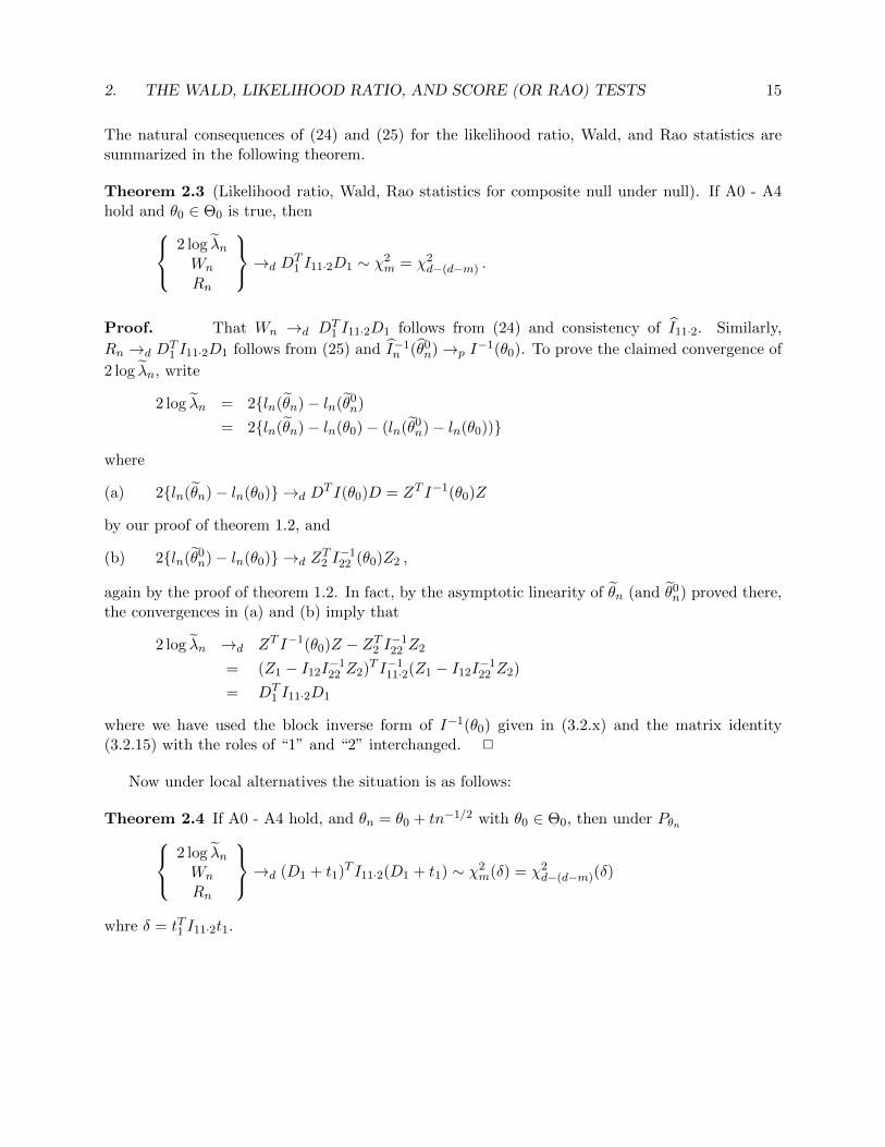
2. THE WALD, LIKELIHOOD RATIO, AND SCORE (OR RAO) TESTS 15
The natural consequences of (24) and (25) for the likelihood ratio, Wald, and Rao statistics aresummarized in the following theorem.
Theorem 2.3 (Likelihood ratio, Wald, Rao statistics for composite null under null). If A0 - A4hold and θ0 ∈ Θ0 is true, then 2 log λn
Wn
Rn
→d DT1 I11·2D1 ∼ χ2
m = χ2d−(d−m) .
Proof. That Wn →d DT1 I11·2D1 follows from (24) and consistency of I11·2. Similarly,
Rn →d DT1 I11·2D1 follows from (25) and I−1
n (θ0n)→p I
−1(θ0). To prove the claimed convergence of
2 log λn, write
2 log λn = 2{ln(θn)− ln(θ0n)
= 2{ln(θn)− ln(θ0)− (ln(θ0n)− ln(θ0))}
where
2{ln(θn)− ln(θ0)} →d DT I(θ0)D = ZT I−1(θ0)Z(a)
by our proof of theorem 1.2, and
2{ln(θ0n)− ln(θ0)} →d Z
T2 I−122 (θ0)Z2 ,(b)
again by the proof of theorem 1.2. In fact, by the asymptotic linearity of θn (and θ0n) proved there,
the convergences in (a) and (b) imply that
2 log λn →d ZT I−1(θ0)Z − ZT2 I−122 Z2
= (Z1 − I12I−122 Z2)T I−1
11·2(Z1 − I12I−122 Z2)
= DT1 I11·2D1
where we have used the block inverse form of I−1(θ0) given in (3.2.x) and the matrix identity(3.2.15) with the roles of “1” and “2” interchanged. 2
Now under local alternatives the situation is as follows:
Theorem 2.4 If A0 - A4 hold, and θn = θ0 + tn−1/2 with θ0 ∈ Θ0, then under Pθn 2 log λnWn
Rn
→d (D1 + t1)T I11·2(D1 + t1) ∼ χ2m(δ) = χ2
d−(d−m)(δ)
whre δ = tT1 I11·2t1.
16 CHAPTER 4. EFFICIENT LIKELIHOOD ESTIMATION AND RELATED TESTS
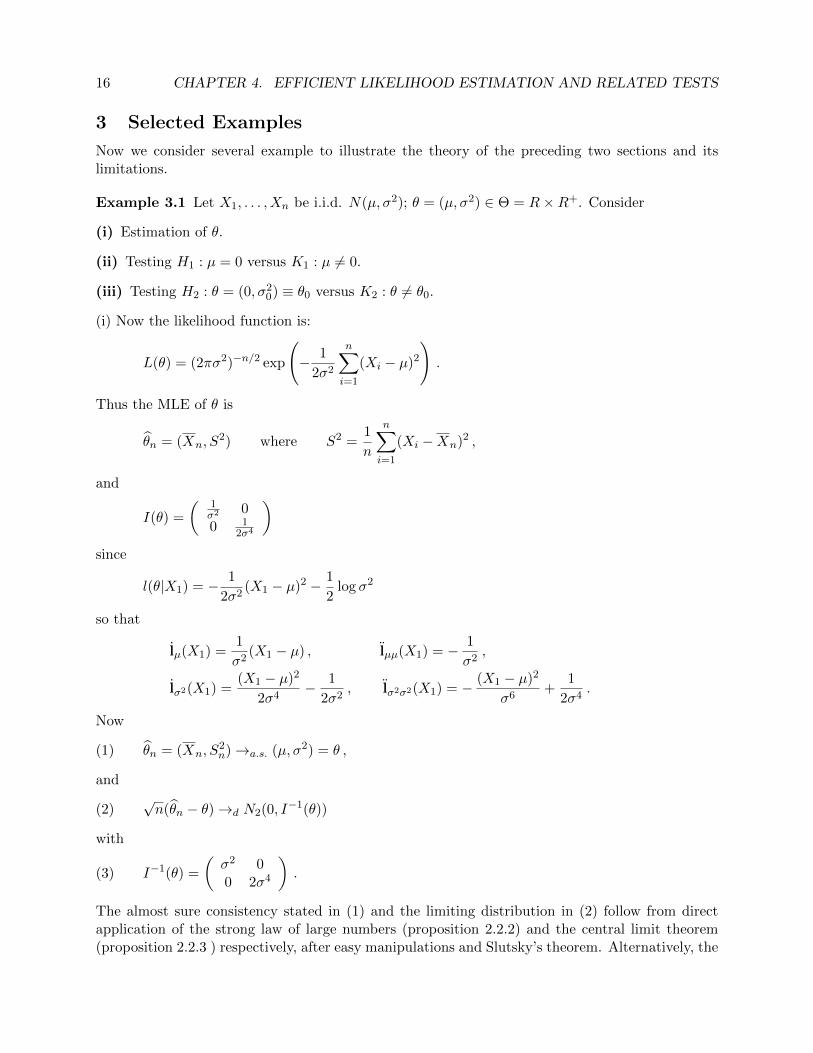
3 Selected Examples
Now we consider several example to illustrate the theory of the preceding two sections and itslimitations.
Example 3.1 Let X1, . . . , Xn be i.i.d. N(µ, σ2); θ = (µ, σ2) ∈ Θ = R×R+. Consider
(i) Estimation of θ.
(ii) Testing H1 : µ = 0 versus K1 : µ 6= 0.
(iii) Testing H2 : θ = (0, σ20) ≡ θ0 versus K2 : θ 6= θ0.
(i) Now the likelihood function is:
L(θ) = (2πσ2)−n/2 exp
(− 1
2σ2
n∑i=1
(Xi − µ)2
).
Thus the MLE of θ is
θn = (Xn, S2) where S2 =
1
n
n∑i=1
(Xi −Xn)2 ,
and
I(θ) =
(1σ2 00 1
2σ4
)since
l(θ|X1) = − 1
2σ2(X1 − µ)2 − 1
2log σ2
so that
lµ(X1) =1
σ2(X1 − µ) , lµµ(X1) = − 1
σ2,
lσ2(X1) =(X1 − µ)2
2σ4− 1
2σ2, lσ2σ2(X1) = − (X1 − µ)2
σ6+
1
2σ4.
Now
θn = (Xn, S2n)→a.s. (µ, σ2) = θ ,(1)
and
√n(θn − θ)→d N2(0, I−1(θ))(2)
with
I−1(θ) =
(σ2 00 2σ4
).(3)
The almost sure consistency stated in (1) and the limiting distribution in (2) follow from directapplication of the strong law of large numbers (proposition 2.2.2) and the central limit theorem(proposition 2.2.3 ) respectively, after easy manipulations and Slutsky’s theorem. Alternatively, the
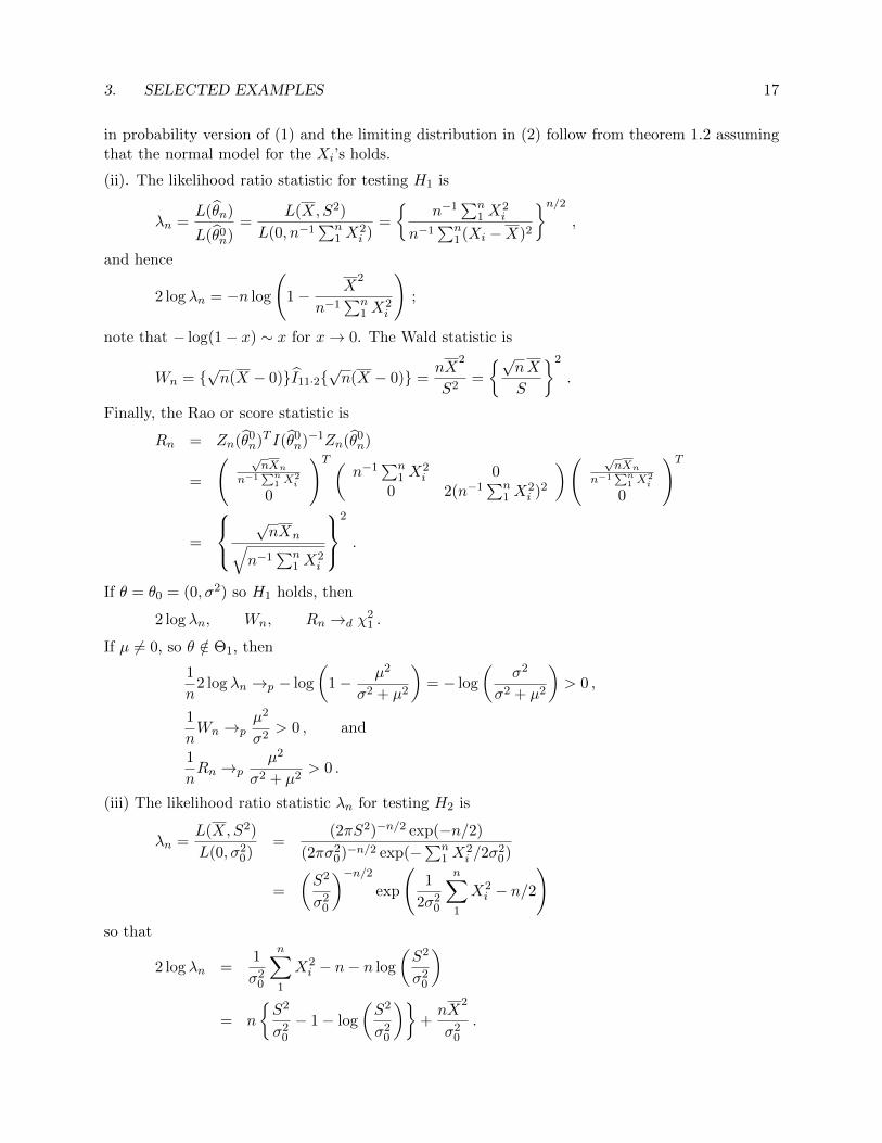
3. SELECTED EXAMPLES 17
in probability version of (1) and the limiting distribution in (2) follow from theorem 1.2 assumingthat the normal model for the Xi’s holds.
(ii). The likelihood ratio statistic for testing H1 is
λn =L(θn)
L(θ0n)
=L(X,S2)
L(0, n−1∑n
1 X2i )
=
{n−1
∑n1 X
2i
n−1∑n
1 (Xi −X)2
}n/2,
and hence
2 log λn = −n log
(1− X
2
n−1∑n
1 X2i
);
note that − log(1− x) ∼ x for x→ 0. The Wald statistic is
Wn = {√n(X − 0)}I11·2{
√n(X − 0)} =
nX2
S2=
{√nX
S
}2
.
Finally, the Rao or score statistic is
Rn = Zn(θ0n)T I(θ0
n)−1Zn(θ0n)
=
( √nXn
n−1∑n
1 X2i
0
)T (n−1
∑n1 X
2i 0
0 2(n−1∑n
1 X2i )2
)( √nXn
n−1∑n
1 X2i
0
)T
=
√nXn√
n−1∑n
1 X2i
2
.
If θ = θ0 = (0, σ2) so H1 holds, then
2 log λn, Wn, Rn →d χ21 .
If µ 6= 0, so θ /∈ Θ1, then
1
n2 log λn →p − log
(1− µ2
σ2 + µ2
)= − log
(σ2
σ2 + µ2
)> 0 ,
1
nWn →p
µ2
σ2> 0 , and
1
nRn →p
µ2
σ2 + µ2> 0 .
(iii) The likelihood ratio statistic λn for testing H2 is
λn =L(X,S2)
L(0, σ20)
=(2πS2)−n/2 exp(−n/2)
(2πσ20)−n/2 exp(−
∑n1 X
2i /2σ
20)
=
(S2
σ20
)−n/2exp
(1
2σ20
n∑1
X2i − n/2
)so that
2 log λn =1
σ20
n∑1
X2i − n− n log
(S2
σ20
)
= n
{S2
σ20
− 1− log
(S2
σ20
)}+nX
2
σ20
.
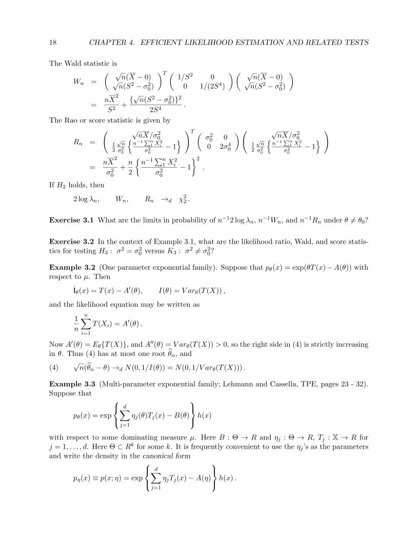
18 CHAPTER 4. EFFICIENT LIKELIHOOD ESTIMATION AND RELATED TESTS
The Wald statistic is
Wn =
( √n(X − 0)√n(S2 − σ2
0)
)T (1/S2 0
0 1/(2S4)
)( √n(X − 0)√n(S2 − σ2
0)
)=
nX2
S2+{√n(S2 − σ2
0)}2
2S4.
The Rao or score statistic is given by
Rn =
( √nX/σ2
012
√n
σ20
{n−1
∑n1 X
2i
σ20
− 1} )T ( σ2
0 00 2σ4
0
)( √nX/σ2
012
√n
σ20
{n−1
∑n1 X
2i
σ20
− 1} )
=nX
2
σ20
+n
2
{n−1
∑n1 X
2i
σ20
− 1
}2
.
If H2 holds, then
2 log λn, Wn, Rn →d χ22 .
Exercise 3.1 What are the limits in probability of n−12 log λn, n−1Wn, and n−1Rn under θ 6= θ0?
Exercise 3.2 In the context of Example 3.1, what are the likelihood ratio, Wald, and score statis-tics for testing H3 : σ2 = σ2
0 versus K3 : σ2 6= σ20?
Example 3.2 (One parameter exponential family). Suppose that pθ(x) = exp(θT (x)−A(θ)) withrespect to µ. Then
lθ(x) = T (x)−A′(θ), I(θ) = V arθ(T (X)) ,
and the likelihood equation may be written as
1
n
n∑i=1
T (Xi) = A′(θ) .
Now A′(θ) = Eθ{T (X)}, and A′′(θ) = V arθ(T (X)) > 0, so the right side in (4) is strictly increasingin θ. Thus (4) has at most one root θn, and
√n(θn − θ)→d N(0, 1/I(θ)) = N(0, 1/V arθ(T (X))) .(4)
Example 3.3 (Multi-parameter exponential family; Lehmann and Cassella, TPE, pages 23 - 32).Suppose that
pθ(x) = exp
d∑j=1
ηj(θ)Tj(x)−B(θ)
h(x)
with respect to some dominating measure µ. Here B : Θ → R and ηj : Θ → R, Tj : X → R forj = 1, . . . , d. Here Θ ⊂ Rk for some k. It is frequently convenient to use the ηj ’s as the parametersand write the density in the canonical form
pη(x) ≡ p(x; η) = exp
d∑j=1
ηjTj(x)−A(η)
h(x) .
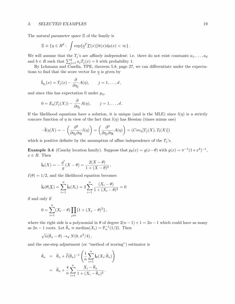
3. SELECTED EXAMPLES 19
The natural parameter space Ξ of the family is
Ξ ≡ {η ∈ Rd :
∫exp{ηTT (x)}h(x)dµ(x) <∞} .
We will assume that the Tj ’s are affinely independent: i.e. there do not exist constants a1, . . . , adand b ∈ R such that
∑dj=1 ajTj(x) = b with probability 1.
By Lehmann and Casella, TPE, theorem 5.8, page 27, we can differentiate under the expecta-tions to find that the score vector for η is given by
lηj (x) = Tj(x)− ∂
∂ηjA(η), j = 1, . . . , d ,
and since this has expectation 0 under pη,
0 = Eη(Tj(X))− ∂
∂ηjA(η), j = 1, . . . , d .
If the likelihood equations have a solution, it is unique (and is the MLE) since l(η) is a strictlyconcave function of η in view of the fact that l(η) has Hessian (times minus one)
−l(η|X) = −(
∂2
∂ηj∂ηll(η)
)=
(∂2
∂ηj∂ηlA(η)
)= (Covη[Tj(X), Tl(X)])
which is positive definite by the assumption of affine independence of the Tj ’s.
Example 3.4 (Cauchy location family). Suppose that pθ(x) = g(x−θ) with g(x) = π−1(1+x2)−1,x ∈ R. Then
lθ(X) = − g′
g(X − θ) =
2(X − θ)1 + (X − θ)2
,
I(θ) = 1/2, and the likelihood equation becomes
lθ(θ|X) =n∑i=1
lθ(Xi) = 2n∑i=1
(Xi − θ)1 + (Xi − θ)2
= 0
if and only if
0 =n∑i=1
(Xi − θ)∏j 6=i{1 + (Xj − θ)2} ,
where the right side is a polynomial in θ of degree 2(n− 1) + 1 = 2n− 1 which could have as manyas 2n− 1 roots. Let θn ≡ median(Xi) = F−1
n (1/2). Then√n(θn − θ)→d N(0, π2/4) ,
and the one-step adjustment (or “method of scoring”) estimator is
θn = θn + I(θn)−1
(1
n
n∑i=1
lθ(Xi; θn)
)
= θn +4
n
n∑i=1
Xi − θn1 + (Xi − θn)2
.
20 CHAPTER 4. EFFICIENT LIKELIHOOD ESTIMATION AND RELATED TESTS
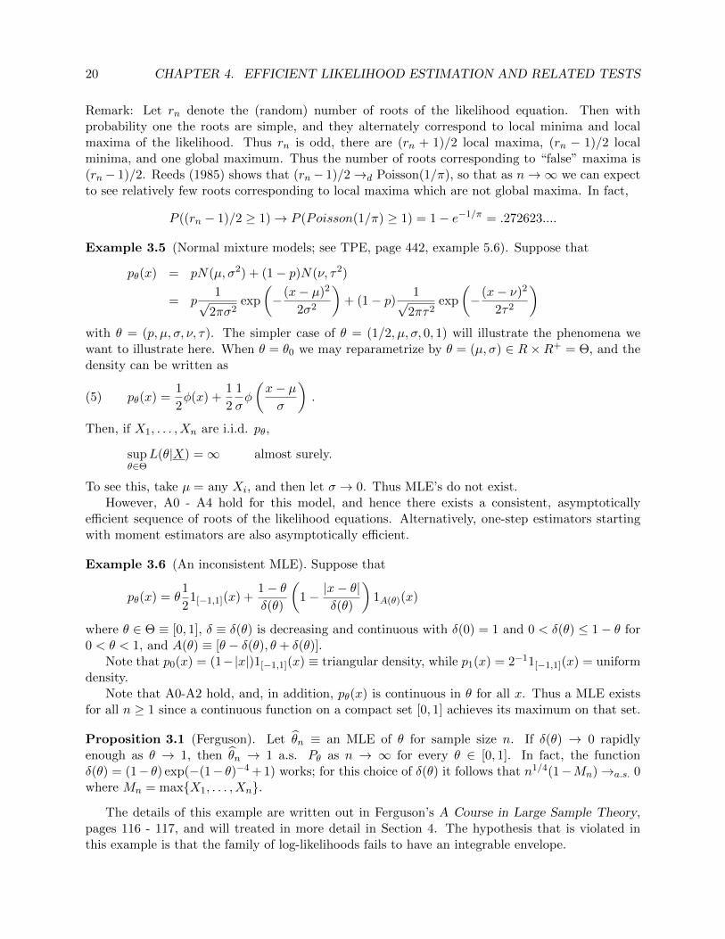
Remark: Let rn denote the (random) number of roots of the likelihood equation. Then withprobability one the roots are simple, and they alternately correspond to local minima and localmaxima of the likelihood. Thus rn is odd, there are (rn + 1)/2 local maxima, (rn − 1)/2 localminima, and one global maximum. Thus the number of roots corresponding to “false” maxima is(rn− 1)/2. Reeds (1985) shows that (rn− 1)/2→d Poisson(1/π), so that as n→∞ we can expectto see relatively few roots corresponding to local maxima which are not global maxima. In fact,
P ((rn − 1)/2 ≥ 1)→ P (Poisson(1/π) ≥ 1) = 1− e−1/π = .272623....
Example 3.5 (Normal mixture models; see TPE, page 442, example 5.6). Suppose that
pθ(x) = pN(µ, σ2) + (1− p)N(ν, τ2)
= p1√
2πσ2exp
(−(x− µ)2
2σ2
)+ (1− p) 1√
2πτ2exp
(−(x− ν)2
2τ2
)with θ = (p, µ, σ, ν, τ). The simpler case of θ = (1/2, µ, σ, 0, 1) will illustrate the phenomena wewant to illustrate here. When θ = θ0 we may reparametrize by θ = (µ, σ) ∈ R×R+ = Θ, and thedensity can be written as
pθ(x) =1
2φ(x) +
1
2
1
σφ
(x− µσ
).(5)
Then, if X1, . . . , Xn are i.i.d. pθ,
supθ∈Θ
L(θ|X) =∞ almost surely.
To see this, take µ = any Xi, and then let σ → 0. Thus MLE’s do not exist.However, A0 - A4 hold for this model, and hence there exists a consistent, asymptotically
efficient sequence of roots of the likelihood equations. Alternatively, one-step estimators startingwith moment estimators are also asymptotically efficient.
Example 3.6 (An inconsistent MLE). Suppose that
pθ(x) = θ1
21[−1,1](x) +
1− θδ(θ)
(1− |x− θ|
δ(θ)
)1A(θ)(x)
where θ ∈ Θ ≡ [0, 1], δ ≡ δ(θ) is decreasing and continuous with δ(0) = 1 and 0 < δ(θ) ≤ 1− θ for0 < θ < 1, and A(θ) ≡ [θ − δ(θ), θ + δ(θ)].
Note that p0(x) = (1−|x|)1[−1,1](x) ≡ triangular density, while p1(x) = 2−11[−1,1](x) = uniformdensity.
Note that A0-A2 hold, and, in addition, pθ(x) is continuous in θ for all x. Thus a MLE existsfor all n ≥ 1 since a continuous function on a compact set [0, 1] achieves its maximum on that set.
Proposition 3.1 (Ferguson). Let θn ≡ an MLE of θ for sample size n. If δ(θ) → 0 rapidlyenough as θ → 1, then θn → 1 a.s. Pθ as n → ∞ for every θ ∈ [0, 1]. In fact, the functionδ(θ) = (1− θ) exp(−(1− θ)−4 + 1) works; for this choice of δ(θ) it follows that n1/4(1−Mn)→a.s. 0where Mn = max{X1, . . . , Xn}.
The details of this example are written out in Ferguson’s A Course in Large Sample Theory,pages 116 - 117, and will treated in more detail in Section 4. The hypothesis that is violated inthis example is that the family of log-likelihoods fails to have an integrable envelope.
3. SELECTED EXAMPLES 21
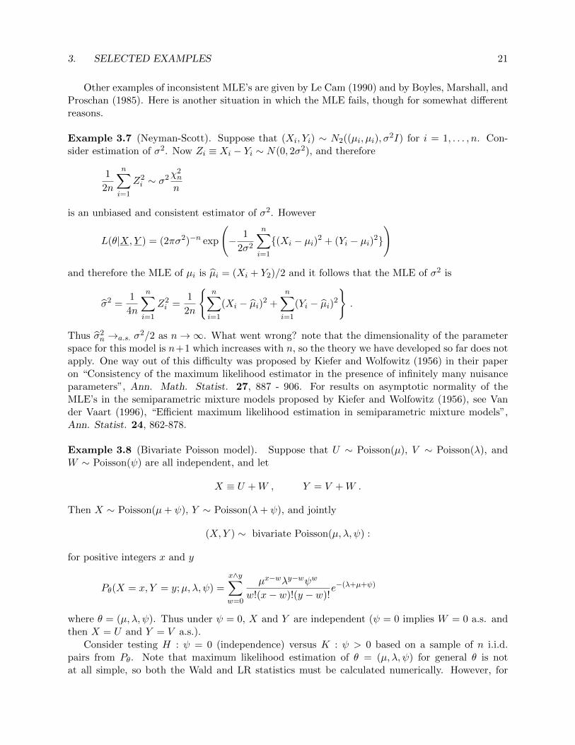
Other examples of inconsistent MLE’s are given by Le Cam (1990) and by Boyles, Marshall, andProschan (1985). Here is another situation in which the MLE fails, though for somewhat differentreasons.
Example 3.7 (Neyman-Scott). Suppose that (Xi, Yi) ∼ N2((µi, µi), σ2I) for i = 1, . . . , n. Con-
sider estimation of σ2. Now Zi ≡ Xi − Yi ∼ N(0, 2σ2), and therefore
1
2n
n∑i=1
Z2i ∼ σ2χ
2n
n
is an unbiased and consistent estimator of σ2. However
L(θ|X,Y ) = (2πσ2)−n exp
(− 1
2σ2
n∑i=1
{(Xi − µi)2 + (Yi − µi)2}
)
and therefore the MLE of µi is µi = (Xi + Y2)/2 and it follows that the MLE of σ2 is
σ2 =1
4n
n∑i=1
Z2i =
1
2n
{n∑i=1
(Xi − µi)2 +n∑i=1
(Yi − µi)2
}.
Thus σ2n →a.s. σ
2/2 as n→∞. What went wrong? note that the dimensionality of the parameterspace for this model is n+1 which increases with n, so the theory we have developed so far does notapply. One way out of this difficulty was proposed by Kiefer and Wolfowitz (1956) in their paperon “Consistency of the maximum likelihood estimator in the presence of infinitely many nuisanceparameters”, Ann. Math. Statist. 27, 887 - 906. For results on asymptotic normality of theMLE’s in the semiparametric mixture models proposed by Kiefer and Wolfowitz (1956), see Vander Vaart (1996), “Efficient maximum likelihood estimation in semiparametric mixture models”,Ann. Statist. 24, 862-878.
Example 3.8 (Bivariate Poisson model). Suppose that U ∼ Poisson(µ), V ∼ Poisson(λ), andW ∼ Poisson(ψ) are all independent, and let
X ≡ U +W , Y = V +W .
Then X ∼ Poisson(µ+ ψ), Y ∼ Poisson(λ+ ψ), and jointly
(X,Y ) ∼ bivariate Poisson(µ, λ, ψ) :
for positive integers x and y
Pθ(X = x, Y = y;µ, λ, ψ) =
x∧y∑w=0
µx−wλy−wψw
w!(x− w)!(y − w)!e−(λ+µ+ψ)
where θ = (µ, λ, ψ). Thus under ψ = 0, X and Y are independent (ψ = 0 implies W = 0 a.s. andthen X = U and Y = V a.s.).
Consider testing H : ψ = 0 (independence) versus K : ψ > 0 based on a sample of n i.i.d.pairs from Pθ. Note that maximum likelihood estimation of θ = (µ, λ, ψ) for general θ is notat all simple, so both the Wald and LR statistics must be calculated numerically. However, for
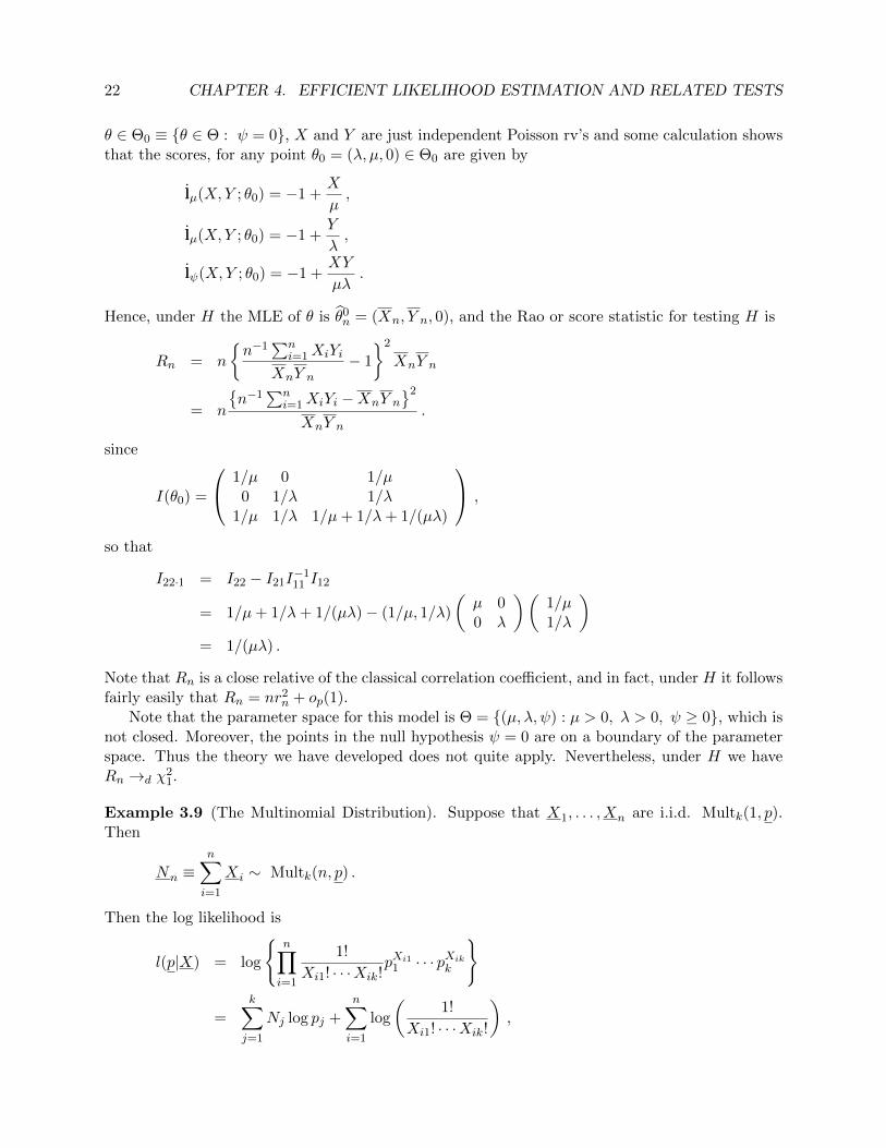
22 CHAPTER 4. EFFICIENT LIKELIHOOD ESTIMATION AND RELATED TESTS
θ ∈ Θ0 ≡ {θ ∈ Θ : ψ = 0}, X and Y are just independent Poisson rv’s and some calculation showsthat the scores, for any point θ0 = (λ, µ, 0) ∈ Θ0 are given by
lµ(X,Y ; θ0) = −1 +X
µ,
lµ(X,Y ; θ0) = −1 +Y
λ,
lψ(X,Y ; θ0) = −1 +XY
µλ.
Hence, under H the MLE of θ is θ0n = (Xn, Y n, 0), and the Rao or score statistic for testing H is
Rn = n
{n−1
∑ni=1XiYi
XnY n
− 1
}2
XnY n
= n
{n−1
∑ni=1XiYi −XnY n
}2
XnY n
.
since
I(θ0) =
1/µ 0 1/µ0 1/λ 1/λ
1/µ 1/λ 1/µ+ 1/λ+ 1/(µλ)
,
so that
I22·1 = I22 − I21I−111 I12
= 1/µ+ 1/λ+ 1/(µλ)− (1/µ, 1/λ)
(µ 00 λ
)(1/µ1/λ
)= 1/(µλ) .
Note that Rn is a close relative of the classical correlation coefficient, and in fact, under H it followsfairly easily that Rn = nr2
n + op(1).Note that the parameter space for this model is Θ = {(µ, λ, ψ) : µ > 0, λ > 0, ψ ≥ 0}, which is
not closed. Moreover, the points in the null hypothesis ψ = 0 are on a boundary of the parameterspace. Thus the theory we have developed does not quite apply. Nevertheless, under H we haveRn →d χ
21.
Example 3.9 (The Multinomial Distribution). Suppose that X1, . . . , Xn are i.i.d. Multk(1, p).Then
Nn ≡n∑i=1
Xi ∼ Multk(n, p) .
Then the log likelihood is
l(p|X) = log
{n∏i=1
1!
Xi1! · · ·Xik!pXi11 · · · pXikk
}
=k∑j=1
Nj log pj +n∑i=1
log
(1!
Xi1! · · ·Xik!
),
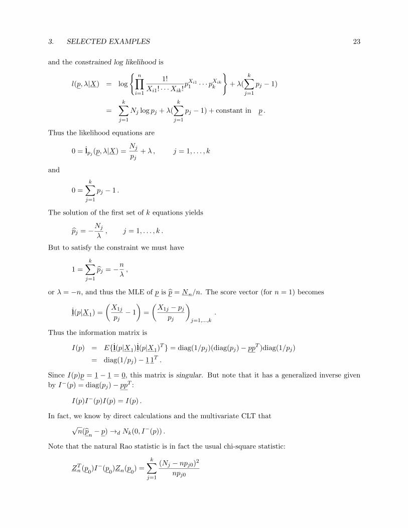
3. SELECTED EXAMPLES 23
and the constrained log likelihood is
l(p, λ|X) = log
{n∏i=1
1!
Xi1! · · ·Xik!pXi11 · · · pXikk
}+ λ(
k∑j=1
pj − 1)
=k∑j=1
Nj log pj + λ(k∑j=1
pj − 1) + constant in p .
Thus the likelihood equations are
0 = lpj (p, λ|X) =Nj
pj+ λ , j = 1, . . . , k
and
0 =
k∑j=1
pj − 1 .
The solution of the first set of k equations yields
pj = −Nj
λ, j = 1, . . . , k .
But to satisfy the constraint we must have
1 =k∑j=1
pj = −nλ,
or λ = −n, and thus the MLE of p is p = Nn/n. The score vector (for n = 1) becomes
l(p|X1) =
(X1j
pj− 1
)=
(X1j − pj
pj
)j=1,...,k
.
Thus the information matrix is
I(p) = E{l(p|X1)l(p|X1)T } = diag(1/pj)(diag(pj)− ppT )diag(1/pj)
= diag(1/pj)− 1 1T .
Since I(p)p = 1 − 1 = 0, this matrix is singular. But note that it has a generalized inverse given
by I−(p) = diag(pj)− ppT :
I(p)I−(p)I(p) = I(p) .
In fact, we know by direct calculations and the multivariate CLT that
√n(p
n− p)→d Nk(0, I
−(p)) .
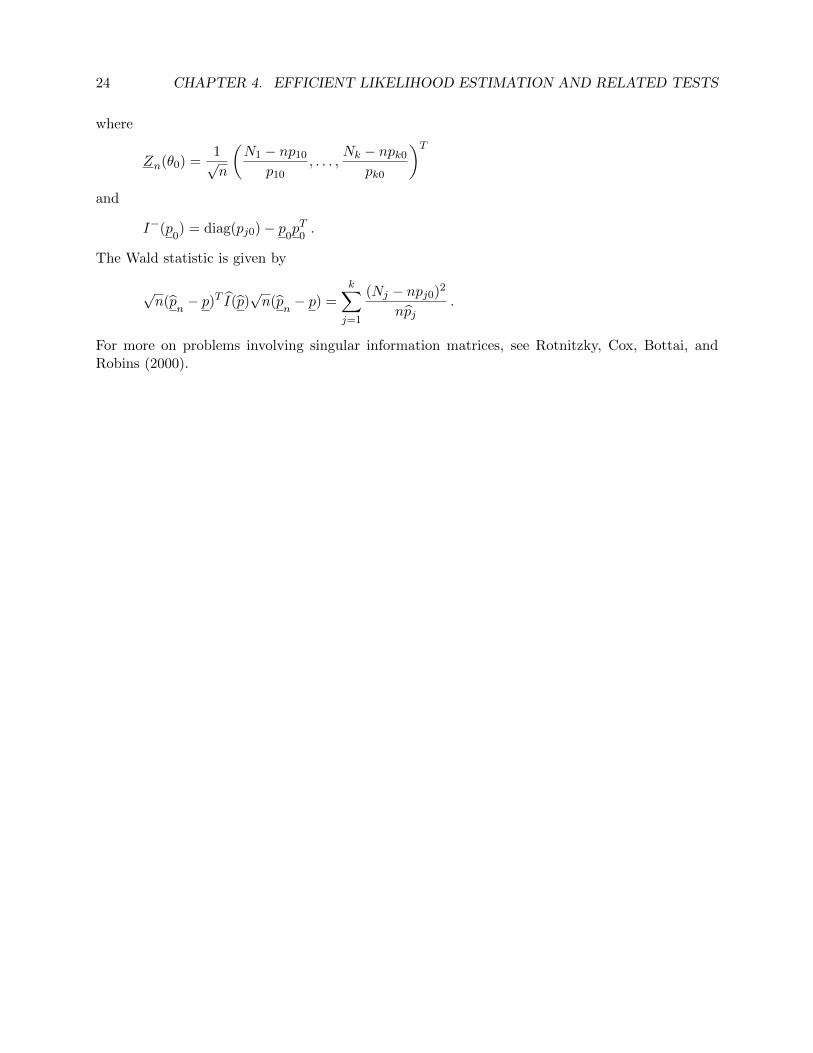
Note that the natural Rao statistic is in fact the usual chi-square statistic:
ZTn (p0)I−(p
0)Zn(p
0) =
k∑j=1
(Nj − npj0)2
npj0
24 CHAPTER 4. EFFICIENT LIKELIHOOD ESTIMATION AND RELATED TESTS
where
Zn(θ0) =1√n
(N1 − np10
p10, . . . ,
Nk − npk0
pk0
)Tand
I−(p0) = diag(pj0)− p
0pT
0.
The Wald statistic is given by
√n(p
n− p)T I(p)
√n(p
n− p) =
k∑j=1
(Nj − npj0)2
npj.
For more on problems involving singular information matrices, see Rotnitzky, Cox, Bottai, andRobins (2000).
4. CONSISTENCY OF MAXIMUM LIKELIHOOD ESTIMATORS 25
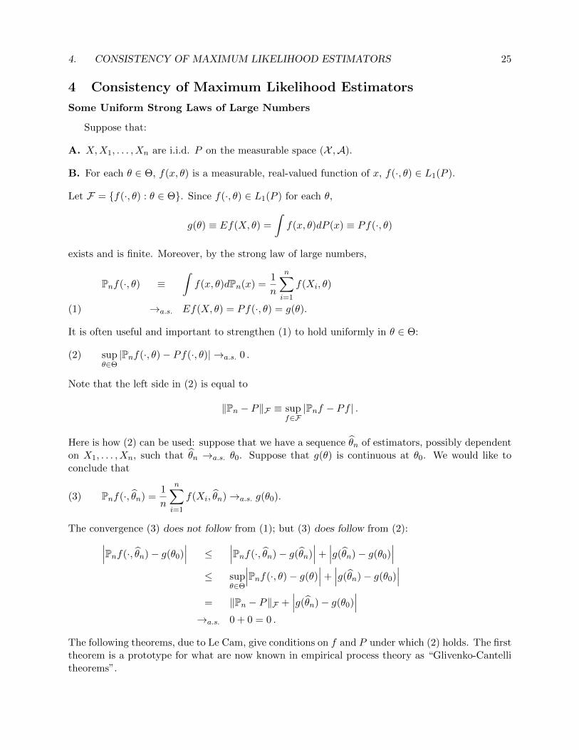
4 Consistency of Maximum Likelihood Estimators
Some Uniform Strong Laws of Large Numbers
Suppose that:
A. X,X1, . . . , Xn are i.i.d. P on the measurable space (X ,A).
B. For each θ ∈ Θ, f(x, θ) is a measurable, real-valued function of x, f(·, θ) ∈ L1(P ).
Let F = {f(·, θ) : θ ∈ Θ}. Since f(·, θ) ∈ L1(P ) for each θ,
g(θ) ≡ Ef(X, θ) =
∫f(x, θ)dP (x) ≡ Pf(·, θ)
exists and is finite. Moreover, by the strong law of large numbers,
Pnf(·, θ) ≡∫f(x, θ)dPn(x) =
1
n
n∑i=1
f(Xi, θ)
→a.s. Ef(X, θ) = Pf(·, θ) = g(θ).(1)
It is often useful and important to strengthen (1) to hold uniformly in θ ∈ Θ:
supθ∈Θ|Pnf(·, θ)− Pf(·, θ)| →a.s. 0 .(2)
Note that the left side in (2) is equal to
‖Pn − P‖F ≡ supf∈F|Pnf − Pf | .
Here is how (2) can be used: suppose that we have a sequence θn of estimators, possibly dependenton X1, . . . , Xn, such that θn →a.s. θ0. Suppose that g(θ) is continuous at θ0. We would like toconclude that
Pnf(·, θn) =1
n
n∑i=1
f(Xi, θn)→a.s. g(θ0).(3)
The convergence (3) does not follow from (1); but (3) does follow from (2):∣∣∣Pnf(·, θn)− g(θ0)∣∣∣ ≤
∣∣∣Pnf(·, θn)− g(θn)∣∣∣+∣∣∣g(θn)− g(θ0)
∣∣∣≤ sup
θ∈Θ
∣∣∣Pnf(·, θ)− g(θ)∣∣∣+∣∣∣g(θn)− g(θ0)
∣∣∣= ‖Pn − P‖F +
∣∣∣g(θn)− g(θ0)∣∣∣
→a.s. 0 + 0 = 0 .
The following theorems, due to Le Cam, give conditions on f and P under which (2) holds. The firsttheorem is a prototype for what are now known in empirical process theory as “Glivenko-Cantellitheorems”.
26 CHAPTER 4. EFFICIENT LIKELIHOOD ESTIMATION AND RELATED TESTS
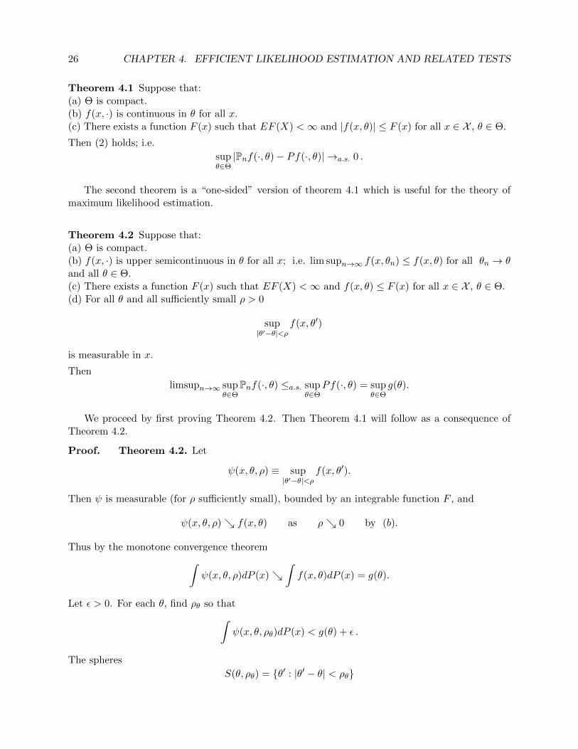
Theorem 4.1 Suppose that:(a) Θ is compact.(b) f(x, ·) is continuous in θ for all x.(c) There exists a function F (x) such that EF (X) <∞ and |f(x, θ)| ≤ F (x) for all x ∈ X , θ ∈ Θ.
Then (2) holds; i.e.
supθ∈Θ|Pnf(·, θ)− Pf(·, θ)| →a.s. 0 .
The second theorem is a “one-sided” version of theorem 4.1 which is useful for the theory ofmaximum likelihood estimation.
Theorem 4.2 Suppose that:(a) Θ is compact.(b) f(x, ·) is upper semicontinuous in θ for all x; i.e. lim supn→∞ f(x, θn) ≤ f(x, θ) for all θn → θand all θ ∈ Θ.(c) There exists a function F (x) such that EF (X) <∞ and f(x, θ) ≤ F (x) for all x ∈ X , θ ∈ Θ.(d) For all θ and all sufficiently small ρ > 0
sup|θ′−θ|<ρ
f(x, θ′)
is measurable in x.
Then
limsupn→∞ supθ∈Θ
Pnf(·, θ) ≤a.s. supθ∈Θ
Pf(·, θ) = supθ∈Θ
g(θ).
We proceed by first proving Theorem 4.2. Then Theorem 4.1 will follow as a consequence ofTheorem 4.2.
Proof. Theorem 4.2. Let
ψ(x, θ, ρ) ≡ sup|θ′−θ|<ρ
f(x, θ′).
Then ψ is measurable (for ρ sufficiently small), bounded by an integrable function F , and
ψ(x, θ, ρ)↘ f(x, θ) as ρ↘ 0 by (b).
Thus by the monotone convergence theorem∫ψ(x, θ, ρ)dP (x)↘
∫f(x, θ)dP (x) = g(θ).
Let ε > 0. For each θ, find ρθ so that∫ψ(x, θ, ρθ)dP (x) < g(θ) + ε .
The spheres
S(θ, ρθ) = {θ′ : |θ′ − θ| < ρθ}
4. CONSISTENCY OF MAXIMUM LIKELIHOOD ESTIMATORS 27
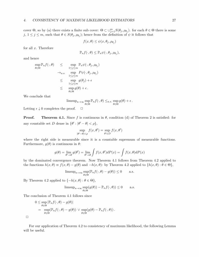
cover Θ, so by (a) there exists a finite sub cover: Θ ⊂ ∪mj=1S(θj , ρθj ). for each θ ∈ Θ there is somej, 1 ≤ j ≤ m, such that θ ∈ S(θj , ρθj ); hence from the definition of ψ it follows that
f(x, θ) ≤ ψ(x, θj , ρθj )
for all x. ThereforePnf(·, θ) ≤ Pnψ(·, θj , ρθj ),
and hence
supθ∈Θ
Pnf(·, θ) ≤ sup1≤j≤m
Pnψ(·, θj , ρθj )
→a.s. sup1≤j≤m
Pψ(·, θj , ρθj )
≤ sup1≤j≤m
g(θj) + ε
≤ supθ∈Θ
g(θ) + ε .
We conclude thatlimsupn→∞ sup
θ∈ΘPnf(·, θ) ≤a.s. sup
θ∈Θg(θ) + ε .
Letting ε ↓ 0 completes the proof. 2
Proof. Theorem 4.1. Since f is continuous in θ, condition (d) of Theorem 2 is satisfied: for
any countable set D dense in {θ′ : |θ′ − θ| < ρ},
sup|θ′−θ|<ρ
f(x, θ′) = supθ′∈D
f(x, θ′)
where the right side is measurable since it is a countable supremum of measurable functions.Furthermore, g(θ) is continuous in θ:
g(θ) = limθ′→θ
g(θ′) = limθ′→θ
∫f(x, θ′)dP (x) =
∫f(x, θ)dP (x)
by the dominated convergence theorem. Now Theorem 4.1 follows from Theorem 4.2 applied tothe functions h(x, θ) ≡ f(x, θ)− g(θ) and −h(x, θ): by Theorem 4.2 applied to {h(x, θ) : θ ∈ Θ},
limsupn→∞ supθ∈Θ
(Pnf(·, θ)− g(θ)) ≤ 0 a.s.
By Theorem 4.2 applied to {−h(x, θ) : θ ∈ Θ},
limsupn→∞ supθ∈Θ
(g(θ))− Pnf(·, θ)) ≤ 0 a.s.
The conclusion of Theorem 4.1 follows since
0 ≤ supθ∈Θ|Pnf(·, θ)− g(θ)|
= supθ∈Θ
(Pnf(·, θ)− g(θ)) ∨ supθ∈Θ
(g(θ)− Pnf(·, θ)) .
2
For our application of Theorem 4.2 to consistency of maximum likelihood, the following Lemmawill be useful.
28 CHAPTER 4. EFFICIENT LIKELIHOOD ESTIMATION AND RELATED TESTS
Lemma 4.1 If the conditions of Theorem 4.2 hold, then g(θ) is upper-semicontinuous: i.e.
limsupθ′→θg(θ′) ≤ g(θ).
Proof. Since f(x, θ) is upper semicontinuous,
limsupθ′→θf(x, θ′) ≤ f(x, θ) for all x ;
i.e.
liminfθ′→θ{f(x, θ)− f(x, θ′)
}≥ 0 for all x .
Hence it follows by Fatou’s lemma that
0 ≤ Eliminfθ′→θ{f(X, θ)− f(X, θ′)
}≤ liminfθ′→θE
{f(X, θ)− f(X, θ′)
}= Ef(X, θ)− limsupθ′→θEf(X, θ′) ;
i.e.
limsupθ′→θEf(X, θ′) ≤ Ef(X, θ) = g(θ) .
2
Now we are prepared to tackle consistency of maximum likelihood estimates.
Theorem 4.3 (Wald, 1949). Suppose that X,X1, . . . , Xn are i.i.d. Pθ0 , θ0 ∈ Θ with densityp(x, θ0) with respect to the dominating measure ν, and that:(a) Θ is compact.(b) p(x, ·) is upper semi-continuous in θ for all x.(c) There exists a function F (x) such that EF (X) <∞ and
f(x, θ) ≡ log p(x, θ)− log p(x, θ0) ≤ F (x)
for all x ∈ X , θ ∈ Θ.(d) For all θ and all sufficiently small ρ > 0
sup|θ′−θ|<ρ
p(x, θ′)
is measurable in x.(e) p(x, θ) = p(x, θ0) a.e. ν implies that θ = θ0.
Then for any sequence of maximum likelihood estimates θn of θ0,
θn →a.s. θ0 .
Proof. Let ρ > 0. The functions {f(x, θ) : θ ∈ Θ} satisfy the conditions of theorem 4.2. Butwe will apply Theorem 4.2 with Θ replaced by the subset
S ≡ {θ : |θ − θ0| ≥ ρ} ⊂ Θ .
4. CONSISTENCY OF MAXIMUM LIKELIHOOD ESTIMATORS 29
Then S is compact, and by Theorem 4.2
Pθ0
(limsupn→∞ sup
θ∈SPnf(·, θ) ≤ sup
θ∈Sg(θ)
)= 1
where
g(θ) = Eθ0f(X, θ) = Eθ0
{log
p(X, θ)
p(X, θ0)
}= −K(Pθ0 , Pθ) < 0 for θ ∈ S.
Furthermore by the Lemma, g(θ) is upper semicontinuous and hence achieves its supremum on thecompact set S. Let δ = supθ∈S g(θ). Then by Lemma 4.1.1 and the identifiability assumption (e),it follows that δ < 0 and we have
Pθ0
(limsupn→∞ sup
θ∈SPnf(·, θ) ≤ δ
)= 1 .
Thus with probability 1 there exists an N such that for all n > N
supθ∈S
Pnf(·, θ) ≤ δ/2 < 0 .
But
Pnf(·, θn) = supθ∈Θ
Pnf(·, θ) = supθ∈Θ
1
n{ln(θ)− ln(θ0)} ≥ 0 .
Hence θn /∈ S for n > N ; that is, |θn − θ0| < ρ with probability 1. Since ρ was arbitrary, θn is a.s.consistent. 2
Remark 4.1 Theorem 4.3 is due to Wald (1949). The present version is an adaptation of Chapters16 and 17 of Ferguson (1996). For further Glivenko - Cantelli theorems, see chapter 2.4 of Van derVaart and Wellner (1996).
30 CHAPTER 4. EFFICIENT LIKELIHOOD ESTIMATION AND RELATED TESTS
5 The EM algorithm
In statistical applications it is a fairly common occurrence that the observations involve “missingdata” or “incomplete data”, and this results in complicated likelihood functions for which there isno explicit formula for the MLE. Our goal in this section is to introduce one quite general scheme formaximizing likelihoods, the EM - algorithm, which is useful for dealing with missing or incompletedata.
Suppose that we observe Y ∼ Qθ on (Y,B) for some θ ∈ Θ; we assume that Qθ has density qθwith respect to a dominating measure ν. This is the “observed” or “incomplete data”.
On the other hand there is often an X ∼ Pθ on (X ,A) which has a simpler likelihood or forwhich the MLE’s can be calculated explicitly, and satisfying Y = T (X). Here we will assume thatPθ has density pθ with respect to µ, and we refer to X as the “unobserved” or “complete data”.Since Y = T (X), it follows that
Qθ(B) = Qθ(Y ∈ B) = Pθ(T (X) ∈ B) = Pθ(X ∈ T−1(B)),
or Qθ = Pθ ◦ T−1. We want to compute
θY = argmaxθ log qθ(Y ),
but this is often difficult because qθ is complicated. We don’t get to observe X, but if we did, thenoften computation of
θX = argmaxθ log pθ(X)
is much easier.
How to proceed? Choose an initial estimator θ(0) of θ, and hence an initial estimator Pθ(0) ofPθ. Then we would proceed via an
E-step: compute, for θ ∈ Θ,
φ0(θ) = φ0(θ, Y ) = EPθ(0){log pθ(X)|T (X) = Y }.
This is the “estimated log-likelihood based on our current guess θ(0) of θ and our observations Y .Then carry out an
M-step: maximize φ0(θ) = φ0(θ, Y ) as a function of θ to find
θ(1) = argmaxφ0(θ).
Now iterate the above two steps:
The following examples illustrate this general scheme.
Example 5.1 (Multinomial). Suppose that Y ∼Mult4(n = 197, p) where
p =
(1
2+θ
4,1− θ
4,1− θ
4,θ
4
), 0 < θ < 1 .
5. THE EM ALGORITHM 31
Therefore
qθ(y) =n!
y1!y2!y3!y4!
(1
2+θ
4
)y1 (1− θ4
)y2 (1− θ4
)y3 (θ4
)y4,
l(θ|Y ) = Y1 log(1/2 + θ/4) + (Y2 + Y3) log(1− θ) + Y4 log θ + constant ,
lθ(Y ) = Y11/4
1/2 + θ/4− (Y2 + Y3)
1
1− θ+ Y4
1
θ,
l(Y ) = −Y1(1/4)2
(1/2 + θ/4)2− (Y2 + Y3)
1
(1− θ)2− Y4
1
θ2,
and
I(θ) =(1/4)2
1/2 + θ/4+
1/2
(1− θ)+
1/4
θ.
If θn is a preliminary estimator of θ, then a one-step estimator of θ is given by
θn = θn + I(θn)−1 1
nl(θn) .
Thus, if Y = (125, 18, 20, 34) is observed, and we take θn = 4Y4/n = (4 · 34)/197 = .6904, then theone-step estimator is
θn = .6904 +1
2.07
1
197(−27.03) = .6904− .0663 = .6241 .
Note that solving the likelihood equation lθ(Y ) = 0 involves solving a cubic equation.
Another approach to maximizing l(θ|Y ) is via the E-M algorithm: suppose the “complete data”is
X ∼Mult5(n, p) with p =
(1
2,θ
4,1− θ
4,1− θ
4,θ
4
).(1)
so that
pθ(x) =n!∏5i=1 xi!
(1
2
)x1 (θ4
)x2+x5 (1− θ4
)x3+x4
,(2)
and the “incomplete data” Y is given in terms of the “complete data” X by
Y = (X1 +X2, X3, X4, X5) .(3)
Then the “E - step” of the algorithm is to estimate X given Y (and θ):
E(X|Y ) =
(Y1
1/2
1/2 + θ/4, Y1
θ/4
1/2 + θ/4, Y2, Y3, Y4
),(4)
so we set
X(p)≡
(Y1
1/2
1/2 + θ(p)/4, Y1
θ(p)/4
1/2 + θ(p)/4, Y2, Y3, Y4
)(5)
where θ(p) is the estimator of θ at the p−th step of the algorithm.
32 CHAPTER 4. EFFICIENT LIKELIHOOD ESTIMATION AND RELATED TESTS
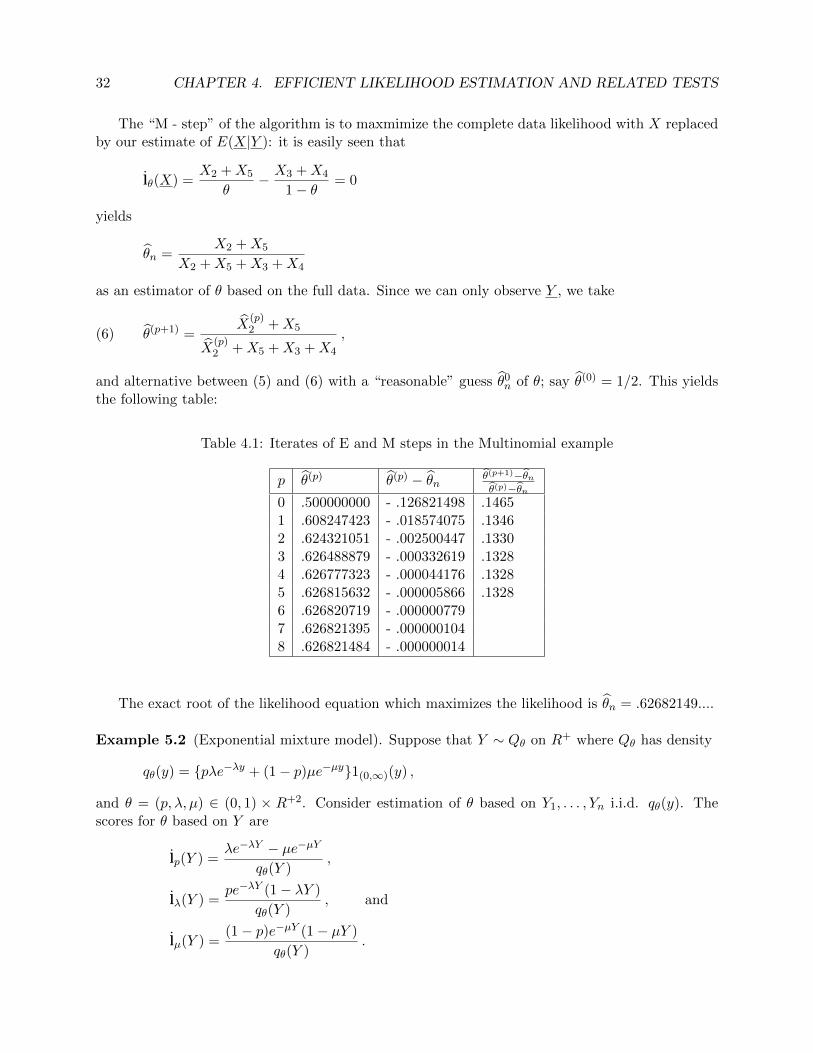
The “M - step” of the algorithm is to maxmimize the complete data likelihood with X replacedby our estimate of E(X|Y ): it is easily seen that
lθ(X) =X2 +X5
θ− X3 +X4
1− θ= 0
yields
θn =X2 +X5
X2 +X5 +X3 +X4
as an estimator of θ based on the full data. Since we can only observe Y , we take
θ(p+1) =X
(p)2 +X5
X(p)2 +X5 +X3 +X4
,(6)
and alternative between (5) and (6) with a “reasonable” guess θ0n of θ; say θ(0) = 1/2. This yields
the following table:
Table 4.1: Iterates of E and M steps in the Multinomial example
p θ(p) θ(p) − θn θ(p+1)−θnθ(p)−θn
0 .500000000 - .126821498 .14651 .608247423 - .018574075 .13462 .624321051 - .002500447 .13303 .626488879 - .000332619 .13284 .626777323 - .000044176 .13285 .626815632 - .000005866 .13286 .626820719 - .0000007797 .626821395 - .0000001048 .626821484 - .000000014
The exact root of the likelihood equation which maximizes the likelihood is θn = .62682149....
Example 5.2 (Exponential mixture model). Suppose that Y ∼ Qθ on R+ where Qθ has density
qθ(y) = {pλe−λy + (1− p)µe−µy}1(0,∞)(y) ,
and θ = (p, λ, µ) ∈ (0, 1) × R+2. Consider estimation of θ based on Y1, . . . , Yn i.i.d. qθ(y). Thescores for θ based on Y are
lp(Y ) =λe−λY − µe−µY
qθ(Y ),
lλ(Y ) =pe−λY (1− λY )
qθ(Y ), and
lµ(Y ) =(1− p)e−µY (1− µY )
qθ(Y ).
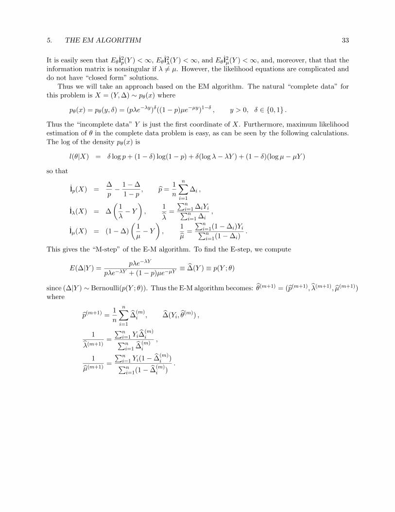
5. THE EM ALGORITHM 33
It is easily seen that Eθ l2p(Y ) <∞, Eθ l
2λ(Y ) <∞, and Eθ l
2µ(Y ) <∞, and, moreover, that that the
information matrix is nonsingular if λ 6= µ. However, the likelihood equations are complicated anddo not have “closed form” solutions.
Thus we will take an approach based on the EM algorithm. The natural “complete data” forthis problem is X = (Y,∆) ∼ pθ(x) where
pθ(x) = pθ(y, δ) = (pλe−λy)δ((1− p)µe−µy)1−δ , y > 0, δ ∈ {0, 1} .
Thus the “incomplete data” Y is just the first coordinate of X. Furthermore, maximum likelihoodestimation of θ in the complete data problem is easy, as can be seen by the following calculations.The log of the density pθ(x) is
l(θ|X) = δ log p+ (1− δ) log(1− p) + δ(log λ− λY ) + (1− δ)(logµ− µY )
so that
lp(X) =∆
p− 1−∆
1− p, p =
1
n
n∑i=1
∆i ,
lλ(X) = ∆
(1
λ− Y
),
1
λ=
∑ni=1 ∆iYi∑ni=1 ∆i
,
lµ(X) = (1−∆)
(1
µ− Y
),
1
µ=
∑ni=1(1−∆i)Yi∑ni=1(1−∆i)
.
This gives the “M-step” of the E-M algorithm. To find the E-step, we compute
E(∆|Y ) =pλe−λY
pλe−λY + (1− p)µe−µY≡ ∆(Y ) ≡ p(Y ; θ)
since (∆|Y ) ∼ Bernoulli(p(Y ; θ)). Thus the E-M algorithm becomes: θ(m+1) = (p(m+1), λ(m+1), µ(m+1))where
p(m+1) =1
n
n∑i=1
∆(m)i , ∆(Yi, θ
(m)) ,
1
λ(m+1)=
∑ni=1 Yi∆
(m)i∑n
i=1 ∆(m)i
,
1
µ(m+1)=
∑ni=1 Yi(1− ∆
(m)i )∑n
i=1(1− ∆(m)i )
.
34 CHAPTER 4. EFFICIENT LIKELIHOOD ESTIMATION AND RELATED TESTS
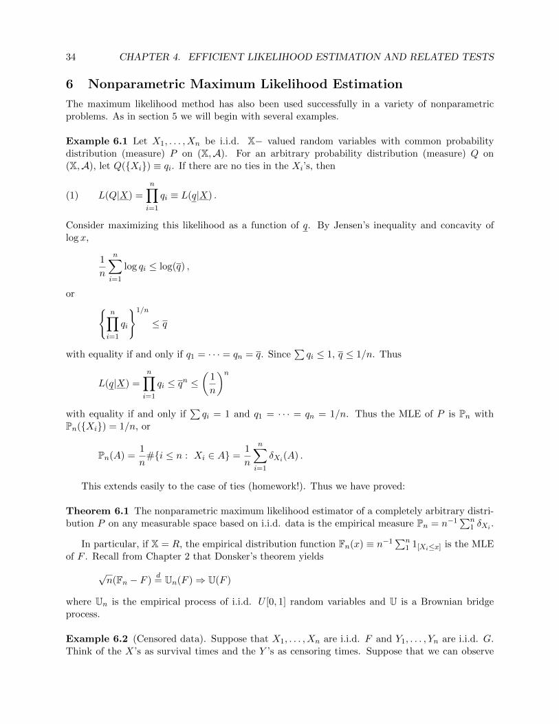
6 Nonparametric Maximum Likelihood Estimation
The maximum likelihood method has also been used successfully in a variety of nonparametricproblems. As in section 5 we will begin with several examples.
Example 6.1 Let X1, . . . , Xn be i.i.d. X− valued random variables with common probabilitydistribution (measure) P on (X,A). For an arbitrary probability distribution (measure) Q on(X,A), let Q({Xi}) ≡ qi. If there are no ties in the Xi’s, then
L(Q|X) =n∏i=1
qi ≡ L(q|X) .(1)
Consider maximizing this likelihood as a function of q. By Jensen’s inequality and concavity oflog x,
1
n
n∑i=1
log qi ≤ log(q) ,
or {n∏i=1
qi
}1/n
≤ q
with equality if and only if q1 = · · · = qn = q. Since∑qi ≤ 1, q ≤ 1/n. Thus
L(q|X) =
n∏i=1
qi ≤ qn ≤(
1
n
)nwith equality if and only if
∑qi = 1 and q1 = · · · = qn = 1/n. Thus the MLE of P is Pn with
Pn({Xi}) = 1/n, or
Pn(A) =1
n#{i ≤ n : Xi ∈ A} =
1
n
n∑i=1
δXi(A) .
This extends easily to the case of ties (homework!). Thus we have proved:
Theorem 6.1 The nonparametric maximum likelihood estimator of a completely arbitrary distri-bution P on any measurable space based on i.i.d. data is the empirical measure Pn = n−1
∑n1 δXi .
In particular, if X = R, the empirical distribution function Fn(x) ≡ n−1∑n
1 1[Xi≤x] is the MLEof F . Recall from Chapter 2 that Donsker’s theorem yields
√n(Fn − F )
d= Un(F )⇒ U(F )
where Un is the empirical process of i.i.d. U [0, 1] random variables and U is a Brownian bridgeprocess.
Example 6.2 (Censored data). Suppose that X1, . . . , Xn are i.i.d. F and Y1, . . . , Yn are i.i.d. G.Think of the X’s as survival times and the Y ’s as censoring times. Suppose that we can observe
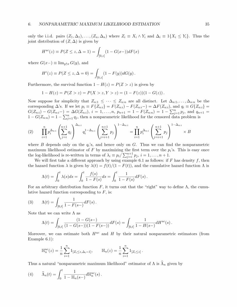
6. NONPARAMETRIC MAXIMUM LIKELIHOOD ESTIMATION 35
only the i.i.d. pairs (Z1,∆1), . . . , (Zn,∆n) where Zi ≡ Xi ∧ Yi and ∆i ≡ 1{Xi ≤ Yi}. Thus thejoint distribution of (Z,∆) is given by
Huc(z) ≡ P (Z ≤ z,∆ = 1) =
∫[0,z]
(1−G(x−))dF (x)
where G(x−) ≡ limy↑xG(y), and
Hc(z) ≡ P (Z ≤ z,∆ = 0) =
∫[0,z]
(1− F (y))dG(y) .
Furthermore, the survival function 1−H(z) = P (Z > z) is given by
1−H(z) = P (Z > z) = P (X > z, Y > z) = (1− F (z))(1−G(z)) .
Now suppose for simplicity that Zn:1 ≤ · · · ≤ Zn:n are all distinct. Let ∆n:1, . . . ,∆n:n be thecorresponding ∆’s. If we let pi ≡ F{Zn:i} = F (Zn:i)− F (Zn:i−) = ∆F (Zn:i), and qi ≡ G{Zn:i} =G(Zn:i) − G(Zn:i−) = ∆G(Zn:i), i = 1, . . . , n, pn+1 = 1 − F (Zn:n) = 1 −
∑nj=1 pj , and qn+1 =
1−G(Zn:n) = 1−∑n
j=1 qj , then a nonparametric likelihood for the censored data problem is
n∏i=1
p∆n:ii
n+1∑j=i
qj
∆n:i
q1−∆n:ii
n+1∑j=i+1
pj
1−∆n:i
=n∏i=1
p∆n:ii
n+1∑j=i+1
pj
1−∆n:i
×B(2)
where B depends only on the qi’s, and hence only on G. Thus we can find the nonparametricmaximum likelihood estimator of F by maximizing the first term over the pi’s. This is easy oncethe log-likelihood is re-written in terms of λi ≡ pi/
∑n+1j=i pj , i = 1, . . . , n+ 1.
We will first take a different approach by using example 6.1 as follows: if F has density f , thenthe hazard function λ is given by λ(t) = f(t)/(1− F (t)), and the cumulative hazard function Λ is
Λ(t) =
∫ t
0λ(s)ds =
∫ t
0
f(s)
1− F (s)ds =
∫ t
0
1
1− F (s)dF (s) .
For an arbitrary distribution function F , it turns out that the “right” way to define Λ, the cumu-lative hazard function corresponding to F , is:
Λ(t) =
∫[0,t]
1
1− F (s−)dF (s) .(3)
Note that we can write Λ as
Λ(t) =
∫[0,t]
(1−G(s−)
(1−G(s−))(1− F (s−))dF (s) =
∫[0,t]
1
1−H(s−)dHuc(s) .
Moreover, we can estimate both Huc and H by their natural nonparametric estimators (fromExample 6.1):
Hucn (z) =
1
n
n∑i=1
1[Zi≤z,∆i=1], Hn(z) =1
n
n∑i=1
1[Zi≤z] .
Thus a natural “nonparametric maximum likelihood” estimator of Λ is Λn given by
Λn(t) =
∫ t
0
1
1−Hn(s−)dHuc
n (s) .(4)
36 CHAPTER 4. EFFICIENT LIKELIHOOD ESTIMATION AND RELATED TESTS
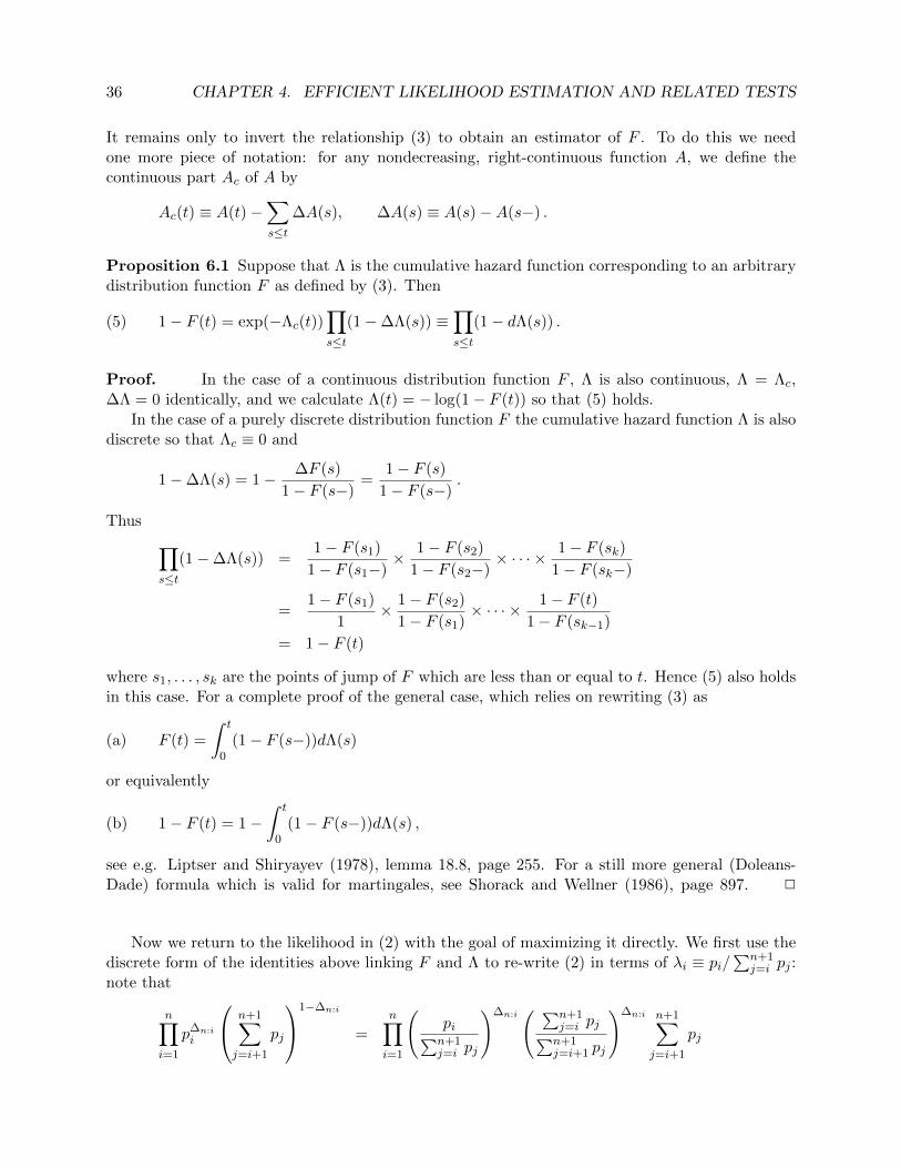
It remains only to invert the relationship (3) to obtain an estimator of F . To do this we needone more piece of notation: for any nondecreasing, right-continuous function A, we define thecontinuous part Ac of A by
Ac(t) ≡ A(t)−∑s≤t
∆A(s), ∆A(s) ≡ A(s)−A(s−) .
Proposition 6.1 Suppose that Λ is the cumulative hazard function corresponding to an arbitrarydistribution function F as defined by (3). Then
1− F (t) = exp(−Λc(t))∏s≤t
(1−∆Λ(s)) ≡∏s≤t
(1− dΛ(s)) .(5)
Proof. In the case of a continuous distribution function F , Λ is also continuous, Λ = Λc,∆Λ = 0 identically, and we calculate Λ(t) = − log(1− F (t)) so that (5) holds.
In the case of a purely discrete distribution function F the cumulative hazard function Λ is alsodiscrete so that Λc ≡ 0 and
1−∆Λ(s) = 1− ∆F (s)
1− F (s−)=
1− F (s)
1− F (s−).
Thus ∏s≤t
(1−∆Λ(s)) =1− F (s1)
1− F (s1−)× 1− F (s2)
1− F (s2−)× · · · × 1− F (sk)
1− F (sk−)
=1− F (s1)
1× 1− F (s2)
1− F (s1)× · · · × 1− F (t)
1− F (sk−1)
= 1− F (t)
where s1, . . . , sk are the points of jump of F which are less than or equal to t. Hence (5) also holdsin this case. For a complete proof of the general case, which relies on rewriting (3) as
F (t) =
∫ t
0(1− F (s−))dΛ(s)(a)
or equivalently
1− F (t) = 1−∫ t
0(1− F (s−))dΛ(s) ,(b)
see e.g. Liptser and Shiryayev (1978), lemma 18.8, page 255. For a still more general (Doleans-Dade) formula which is valid for martingales, see Shorack and Wellner (1986), page 897. 2
Now we return to the likelihood in (2) with the goal of maximizing it directly. We first use thediscrete form of the identities above linking F and Λ to re-write (2) in terms of λi ≡ pi/
∑n+1j=i pj :
note that
n∏i=1
p∆n:ii
n+1∑j=i+1
pj
1−∆n:i
=
n∏i=1
(pi∑n+1j=i pj
)∆n:i( ∑n+1
j=i pj∑n+1j=i+1 pj
)∆n:i n+1∑j=i+1
pj
6. NONPARAMETRIC MAXIMUM LIKELIHOOD ESTIMATION 37
=
n∏i=1
λ∆n:ii (1− λi)−∆n:i
n+1∑j=i+1
pj
since 1− λi = 1− pi∑n+1
j=i pj=
∑n+1j=i+1 pj∑n+1j=i pj
=
n∏i=1
λ∆n:ii (1− λi)−∆n:i ·
n∏i=1
i∏j=1
(1− λj)
since
i∏j=1
(1− λj) =
n+1∑j=i+1
pj
=
n∏i=1
λ∆n:ii (1− λi)−∆n:i
n∏j=1
(1− λj)n−j+1
=n∏i=1
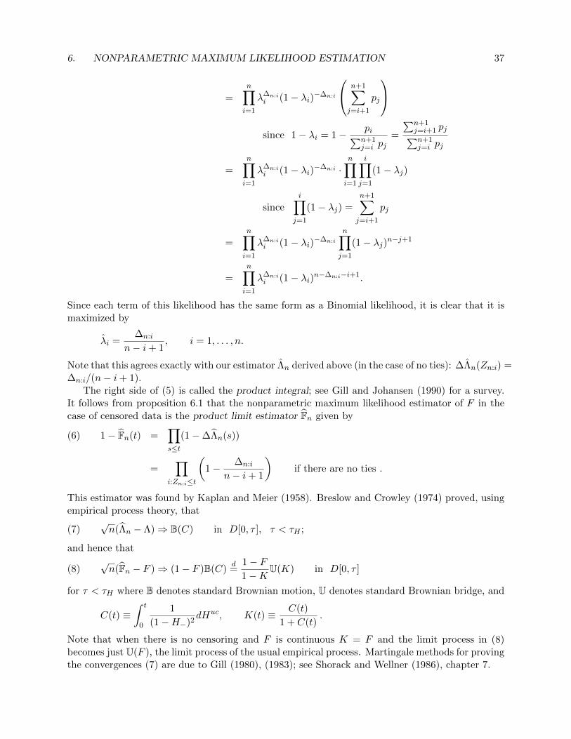
λ∆n:ii (1− λi)n−∆n:i−i+1.
Since each term of this likelihood has the same form as a Binomial likelihood, it is clear that it ismaximized by
λi =∆n:i
n− i+ 1, i = 1, . . . , n.
Note that this agrees exactly with our estimator Λn derived above (in the case of no ties): ∆Λn(Zn:i) =∆n:i/(n− i+ 1).
The right side of (5) is called the product integral; see Gill and Johansen (1990) for a survey.It follows from proposition 6.1 that the nonparametric maximum likelihood estimator of F in thecase of censored data is the product limit estimator Fn given by
1− Fn(t) =∏s≤t
(1−∆Λn(s))(6)
=∏
i:Zn:i≤t
(1− ∆n:i
n− i+ 1
)if there are no ties .
This estimator was found by Kaplan and Meier (1958). Breslow and Crowley (1974) proved, usingempirical process theory, that
√n(Λn − Λ)⇒ B(C) in D[0, τ ], τ < τH ;(7)
and hence that
√n(Fn − F )⇒ (1− F )B(C)
d=
1− F1−K
U(K) in D[0, τ ](8)
for τ < τH where B denotes standard Brownian motion, U denotes standard Brownian bridge, and
C(t) ≡∫ t
0
1
(1−H−)2dHuc, K(t) ≡ C(t)
1 + C(t).
Note that when there is no censoring and F is continuous K = F and the limit process in (8)becomes just U(F ), the limit process of the usual empirical process. Martingale methods for provingthe convergences (7) are due to Gill (1980), (1983); see Shorack and Wellner (1986), chapter 7.
38 CHAPTER 4. EFFICIENT LIKELIHOOD ESTIMATION AND RELATED TESTS
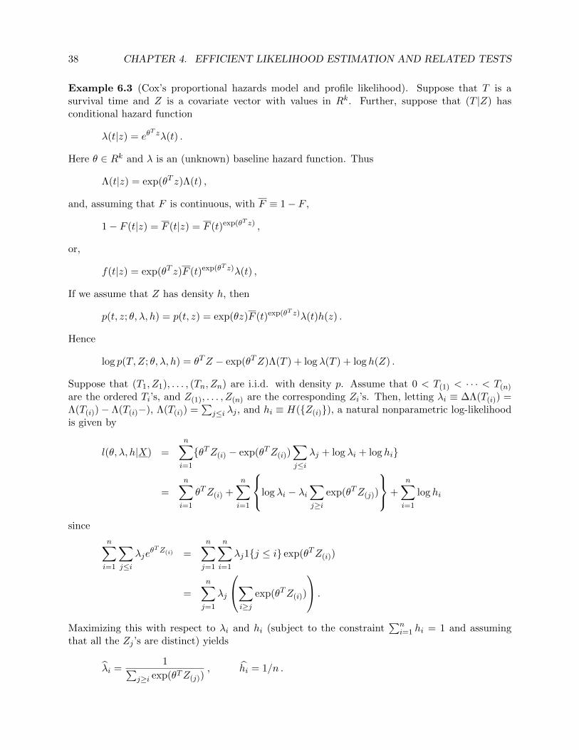
Example 6.3 (Cox’s proportional hazards model and profile likelihood). Suppose that T is asurvival time and Z is a covariate vector with values in Rk. Further, suppose that (T |Z) hasconditional hazard function
λ(t|z) = eθT zλ(t) .
Here θ ∈ Rk and λ is an (unknown) baseline hazard function. Thus
Λ(t|z) = exp(θT z)Λ(t) ,
and, assuming that F is continuous, with F ≡ 1− F ,
1− F (t|z) = F (t|z) = F (t)exp(θT z) ,
or,
f(t|z) = exp(θT z)F (t)exp(θT z)λ(t) ,
If we assume that Z has density h, then
p(t, z; θ, λ, h) = p(t, z) = exp(θz)F (t)exp(θT z)λ(t)h(z) .
Hence
log p(T,Z; θ, λ, h) = θTZ − exp(θTZ)Λ(T ) + log λ(T ) + log h(Z) .
Suppose that (T1, Z1), . . . , (Tn, Zn) are i.i.d. with density p. Assume that 0 < T(1) < · · · < T(n)
are the ordered Ti’s, and Z(1), . . . , Z(n) are the corresponding Zi’s. Then, letting λi ≡ ∆Λ(T(i)) =Λ(T(i))− Λ(T(i)−), Λ(T(i)) =
∑j≤i λj , and hi ≡ H({Z(i)}), a natural nonparametric log-likelihood
is given by
l(θ, λ, h|X) =
n∑i=1
{θTZ(i) − exp(θTZ(i))∑j≤i
λj + log λi + log hi}
=
n∑i=1
θTZ(i) +
n∑i=1
log λi − λi∑j≥i
exp(θTZ(j))
+
n∑i=1
log hi
since
n∑i=1
∑j≤i
λjeθTZ(i) =
n∑j=1
n∑i=1
λj1{j ≤ i} exp(θTZ(i))
=n∑j=1
λj
∑i≥j
exp(θTZ(i))
.
Maximizing this with respect to λi and hi (subject to the constraint∑n
i=1 hi = 1 and assumingthat all the Zj ’s are distinct) yields
λi =1∑
j≥i exp(θTZ(j)), hi = 1/n .
6. NONPARAMETRIC MAXIMUM LIKELIHOOD ESTIMATION 39
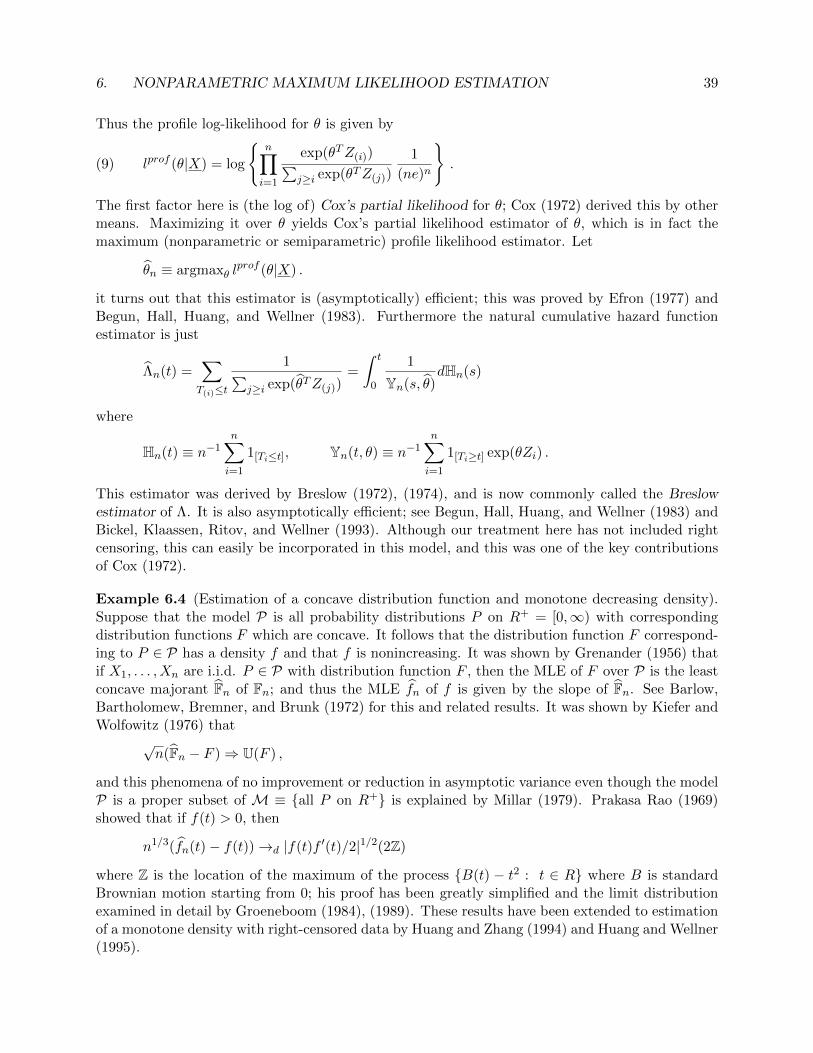
Thus the profile log-likelihood for θ is given by
lprof (θ|X) = log
{n∏i=1
exp(θTZ(i))∑j≥i exp(θTZ(j))
1
(ne)n
}.(9)
The first factor here is (the log of) Cox’s partial likelihood for θ; Cox (1972) derived this by othermeans. Maximizing it over θ yields Cox’s partial likelihood estimator of θ, which is in fact themaximum (nonparametric or semiparametric) profile likelihood estimator. Let
θn ≡ argmaxθ lprof (θ|X) .
it turns out that this estimator is (asymptotically) efficient; this was proved by Efron (1977) andBegun, Hall, Huang, and Wellner (1983). Furthermore the natural cumulative hazard functionestimator is just
Λn(t) =∑T(i)≤t
1∑j≥i exp(θTZ(j))
=
∫ t
0
1
Yn(s, θ)dHn(s)
where
Hn(t) ≡ n−1n∑i=1
1[Ti≤t], Yn(t, θ) ≡ n−1n∑i=1
1[Ti≥t] exp(θZi) .
This estimator was derived by Breslow (1972), (1974), and is now commonly called the Breslowestimator of Λ. It is also asymptotically efficient; see Begun, Hall, Huang, and Wellner (1983) andBickel, Klaassen, Ritov, and Wellner (1993). Although our treatment here has not included rightcensoring, this can easily be incorporated in this model, and this was one of the key contributionsof Cox (1972).
Example 6.4 (Estimation of a concave distribution function and monotone decreasing density).Suppose that the model P is all probability distributions P on R+ = [0,∞) with correspondingdistribution functions F which are concave. It follows that the distribution function F correspond-ing to P ∈ P has a density f and that f is nonincreasing. It was shown by Grenander (1956) thatif X1, . . . , Xn are i.i.d. P ∈ P with distribution function F , then the MLE of F over P is the leastconcave majorant Fn of Fn; and thus the MLE fn of f is given by the slope of Fn. See Barlow,Bartholomew, Bremner, and Brunk (1972) for this and related results. It was shown by Kiefer andWolfowitz (1976) that
√n(Fn − F )⇒ U(F ) ,
and this phenomena of no improvement or reduction in asymptotic variance even though the modelP is a proper subset of M ≡ {all P on R+} is explained by Millar (1979). Prakasa Rao (1969)showed that if f(t) > 0, then
n1/3(fn(t)− f(t))→d |f(t)f ′(t)/2|1/2(2Z)
where Z is the location of the maximum of the process {B(t) − t2 : t ∈ R} where B is standardBrownian motion starting from 0; his proof has been greatly simplified and the limit distributionexamined in detail by Groeneboom (1984), (1989). These results have been extended to estimationof a monotone density with right-censored data by Huang and Zhang (1994) and Huang and Wellner(1995).
40 CHAPTER 4. EFFICIENT LIKELIHOOD ESTIMATION AND RELATED TESTS
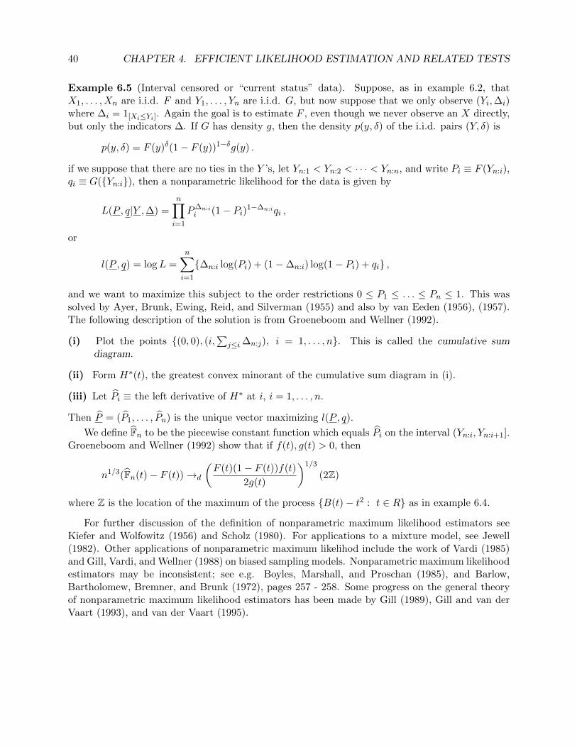
Example 6.5 (Interval censored or “current status” data). Suppose, as in example 6.2, thatX1, . . . , Xn are i.i.d. F and Y1, . . . , Yn are i.i.d. G, but now suppose that we only observe (Yi,∆i)where ∆i = 1[Xi≤Yi]. Again the goal is to estimate F , even though we never observe an X directly,but only the indicators ∆. If G has density g, then the density p(y, δ) of the i.i.d. pairs (Y, δ) is
p(y, δ) = F (y)δ(1− F (y))1−δg(y) .
if we suppose that there are no ties in the Y ’s, let Yn:1 < Yn:2 < · · · < Yn:n, and write Pi ≡ F (Yn:i),qi ≡ G({Yn:i}), then a nonparametric likelihood for the data is given by
L(P , q|Y ,∆) =n∏i=1
P∆n:ii (1− Pi)1−∆n:iqi ,
or
l(P , q) = logL =
n∑i=1
{∆n:i log(Pi) + (1−∆n:i) log(1− Pi) + qi} ,
and we want to maximize this subject to the order restrictions 0 ≤ P1 ≤ . . . ≤ Pn ≤ 1. This wassolved by Ayer, Brunk, Ewing, Reid, and Silverman (1955) and also by van Eeden (1956), (1957).The following description of the solution is from Groeneboom and Wellner (1992).
(i) Plot the points {(0, 0), (i,∑
j≤i ∆n:j), i = 1, . . . , n}. This is called the cumulative sumdiagram.
(ii) Form H∗(t), the greatest convex minorant of the cumulative sum diagram in (i).
(iii) Let Pi ≡ the left derivative of H∗ at i, i = 1, . . . , n.
Then P = (P1, . . . , Pn) is the unique vector maximizing l(P , q).
We define Fn to be the piecewise constant function which equals Pi on the interval (Yn:i, Yn:i+1].Groeneboom and Wellner (1992) show that if f(t), g(t) > 0, then
n1/3(Fn(t)− F (t))→d
(F (t)(1− F (t))f(t)
2g(t)
)1/3
(2Z)
where Z is the location of the maximum of the process {B(t)− t2 : t ∈ R} as in example 6.4.
For further discussion of the definition of nonparametric maximum likelihood estimators seeKiefer and Wolfowitz (1956) and Scholz (1980). For applications to a mixture model, see Jewell(1982). Other applications of nonparametric maximum likelihod include the work of Vardi (1985)and Gill, Vardi, and Wellner (1988) on biased sampling models. Nonparametric maximum likelihoodestimators may be inconsistent; see e.g. Boyles, Marshall, and Proschan (1985), and Barlow,Bartholomew, Bremner, and Brunk (1972), pages 257 - 258. Some progress on the general theoryof nonparametric maximum likelihood estimators has been made by Gill (1989), Gill and van derVaart (1993), and van der Vaart (1995).
7. LIMIT THEORY FOR THE STATISTICAL AGNOSTIC 41
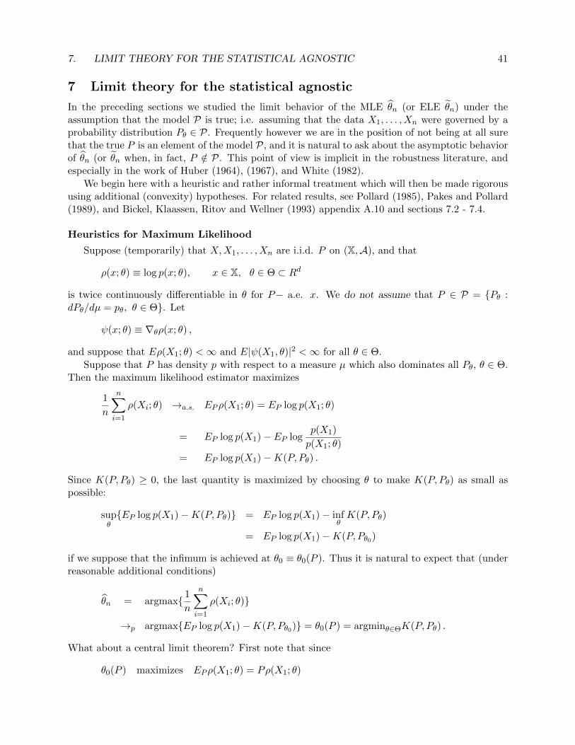
7 Limit theory for the statistical agnostic
In the preceding sections we studied the limit behavior of the MLE θn (or ELE θn) under theassumption that the model P is true; i.e. assuming that the data X1, . . . , Xn were governed by aprobability distribution Pθ ∈ P. Frequently however we are in the position of not being at all surethat the true P is an element of the model P, and it is natural to ask about the asymptotic behaviorof θn (or θn when, in fact, P /∈ P. This point of view is implicit in the robustness literature, andespecially in the work of Huber (1964), (1967), and White (1982).
We begin here with a heuristic and rather informal treatment which will then be made rigoroususing additional (convexity) hypotheses. For related results, see Pollard (1985), Pakes and Pollard(1989), and Bickel, Klaassen, Ritov and Wellner (1993) appendix A.10 and sections 7.2 - 7.4.
Heuristics for Maximum Likelihood
Suppose (temporarily) that X,X1, . . . , Xn are i.i.d. P on (X,A), and that
ρ(x; θ) ≡ log p(x; θ), x ∈ X, θ ∈ Θ ⊂ Rd
is twice continuously differentiable in θ for P− a.e. x. We do not assume that P ∈ P = {Pθ :dPθ/dµ = pθ, θ ∈ Θ}. Let
ψ(x; θ) ≡ ∇θρ(x; θ) ,
and suppose that Eρ(X1; θ) <∞ and E|ψ(X1, θ)|2 <∞ for all θ ∈ Θ.
Suppose that P has density p with respect to a measure µ which also dominates all Pθ, θ ∈ Θ.Then the maximum likelihood estimator maximizes
1
n
n∑i=1
ρ(Xi; θ) →a.s. EPρ(X1; θ) = EP log p(X1; θ)
= EP log p(X1)− EP logp(X1)
p(X1; θ)
= EP log p(X1)−K(P, Pθ) .
Since K(P, Pθ) ≥ 0, the last quantity is maximized by choosing θ to make K(P, Pθ) as small aspossible:
supθ{EP log p(X1)−K(P, Pθ)} = EP log p(X1)− inf
θK(P, Pθ)
= EP log p(X1)−K(P, Pθ0)
if we suppose that the infimum is achieved at θ0 ≡ θ0(P ). Thus it is natural to expect that (underreasonable additional conditions)
θn = argmax{ 1
n
n∑i=1
ρ(Xi; θ)}
→p argmax{EP log p(X1)−K(P, Pθ0)} = θ0(P ) = argminθ∈ΘK(P, Pθ) .
What about a central limit theorem? First note that since
θ0(P ) maximizes EPρ(X1; θ) = Pρ(X1; θ)
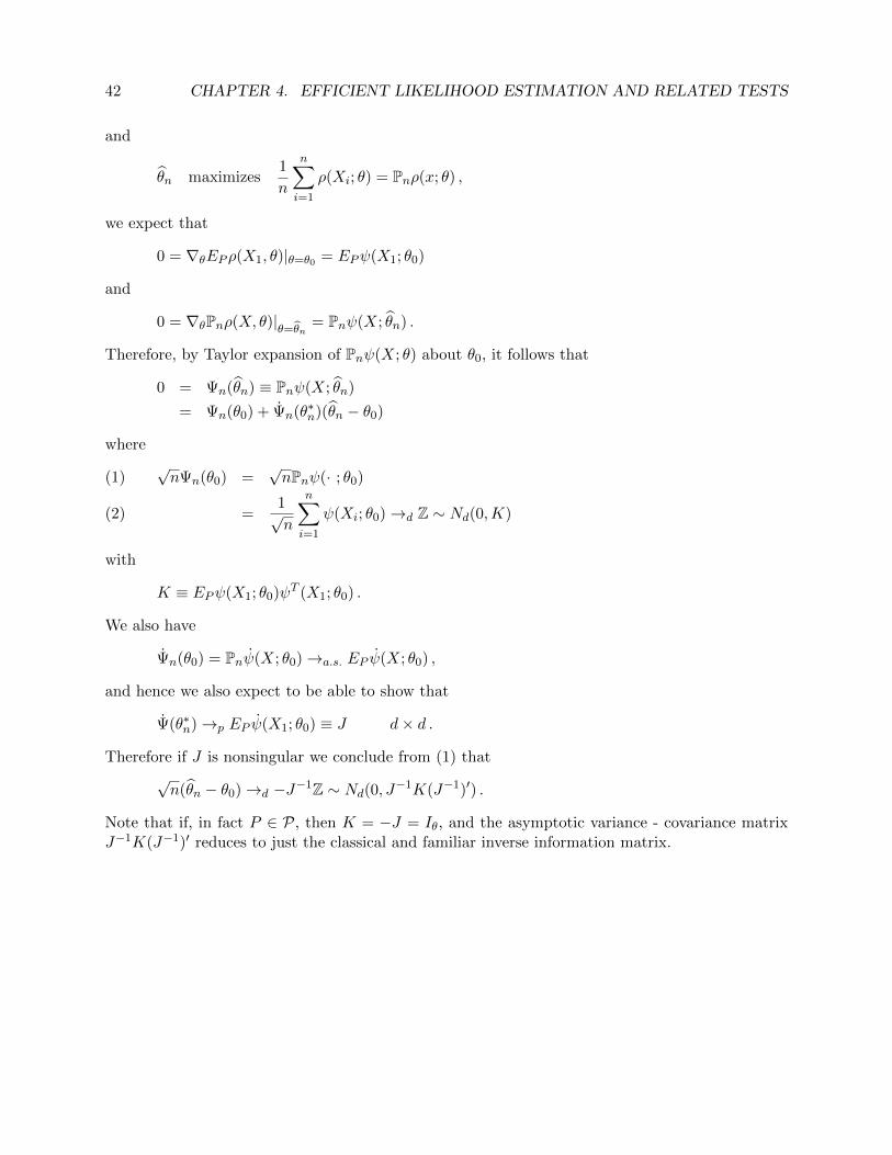
42 CHAPTER 4. EFFICIENT LIKELIHOOD ESTIMATION AND RELATED TESTS
and
θn maximizes1
n
n∑i=1
ρ(Xi; θ) = Pnρ(x; θ) ,
we expect that
0 = ∇θEPρ(X1, θ)|θ=θ0 = EPψ(X1; θ0)
and
0 = ∇θPnρ(X, θ)|θ=θn
= Pnψ(X; θn) .
Therefore, by Taylor expansion of Pnψ(X; θ) about θ0, it follows that
0 = Ψn(θn) ≡ Pnψ(X; θn)
= Ψn(θ0) + Ψn(θ∗n)(θn − θ0)
where
√nΨn(θ0) =
√nPnψ(· ; θ0)(1)
=1√n
n∑i=1
ψ(Xi; θ0)→d Z ∼ Nd(0,K)(2)
with
K ≡ EPψ(X1; θ0)ψT (X1; θ0) .
We also have
Ψn(θ0) = Pnψ(X; θ0)→a.s. EP ψ(X; θ0) ,
and hence we also expect to be able to show that
Ψ(θ∗n)→p EP ψ(X1; θ0) ≡ J d× d .
Therefore if J is nonsingular we conclude from (1) that
√n(θn − θ0)→d −J−1Z ∼ Nd(0, J
−1K(J−1)′) .
Note that if, in fact P ∈ P, then K = −J = Iθ, and the asymptotic variance - covariance matrixJ−1K(J−1)′ reduces to just the classical and familiar inverse information matrix.