Special issue computers & geosciences - CORE · PDF filesampling theory (Spiegel and Stephens,...

ACCEPTED VERSION

Pardo-Iguzquiza, Eulogio; Dowd, Peter Alan Comparison of inference methods for estimating semivariogram model parameters and their uncertainty: The case of small data sets Computers & Geosciences, 2013; 50:154-164

© 2012 Elsevier Ltd. All rights reserved.

NOTICE: this is the author’s version of a work that was accepted for publication in Computers & Geosciences. Changes resulting from the publishing process, such as peer review, editing, corrections, structural formatting, and other quality control mechanisms may not be reflected in this document. Changes may have been made to this work since it was submitted for publication. A definitive version was subsequently published in Computers & Geosciences, 2013; 50:154-164. DOI: 10.1016/j.cageo.2012.06.002

http://hdl.handle.net/2440/78507

PERMISSIONS

http://www.elsevier.com/journal-authors/author-rights-and-responsibilities#author-posting

Elsevier's AAM Policy: Authors retain the right to use the accepted author manuscript for personal use, internal institutional use and for permitted scholarly posting provided that these are not for purposes of commercial use or systematic distribution.

27 August 2013



http://dx.doi.org/10.1016/j.cageo.2012.06.002




1

Comparison of inference methods for

estimating semivariogram model parameters

and their uncertainty:

the case of small data sets

Eulogio Pardo-Igúzquiza 1 and Peter A. Dowd 2

1 Instituto Geológico y Minero de España (IGME).

Geological Survey of Spain.

Ríos Rosas 23, 28003 Madrid, Spain

[email protected]

2 Faculty of Engineering, Computer and Mathematical Sciences,

University of Adelaide, Adelaide, SA 5000, Australia

[email protected]

Abstract

The semivariogram model is the fundamental component in all geostatistical

applications and its inference is an issue of significant practical interest. The

semivariogram model is defined by a mathematical function, the parameters of which

are usually estimated from the experimental data. There are important application areas

mailto:[email protected]

mailto:[email protected]

2

in which small data sets are the norm; rainfall estimation from rain gauge data and

transmissivity estimation from pumping test data are two examples from, respectively,

surface and subsurface hydrology. Thus a benchmark problem in geostatistics is

deciding on the most appropriate method for the inference of the semivariogram model.

The various methods for semivariogram inference can be classified as indirect methods,

in which there is an intermediate step of calculating the experimental semivariogram,

and direct approaches that obtain the model parameter values directly as the values that

minimize some objective function.

To avoid subjectivity in fitting models to experimental semivariograms, ordinary least

squares (OLS), weighted least squares (WLS) and generalized least squares (GLS) are

often used. Uncertainty evaluation in indirect methods is done using computationally

intensive resampling procedures such as the bootstrap method.

Direct methods include parametric methods, such as maximum likelihood (ML) and

maximum likelihood cross-validation (MLCV), and non-parametric methods, such as

minimization of cross-validation statistics (CV).

The bases for comparing the previous methods are the sampling distribution of the

various parameters and the “goodness” of the uncertainty evaluation in a sense that we

define. The final questions to be answered are (1) which is the best method for

estimating each of the three parameters? (2) which is the best method for assessing the

uncertainty of each of the three parameters? (3) which method best selects the

functional form of the semivariogram from among a set of options? and (4) which is

the best method that jointly addresses all the previous questions?

3

Key words: maximum likelihood, cross-validation, least squares, chi-squared field,

root mean square error

1. Introduction

Since the early applications of geostatistics in mining (Matheron, 1963), the range of

applications has been extended significantly to include hydrogeology (e.g. Kitanidis,

1997), petroleum geology (e.g. Deutsch, 2002; Caers, 2005), meteorology and

climatology (e.g. Diodato and Ceccarelli, 2005), soil science (e.g. Goovaerst, 1997),

remote sensing (e.g. Curran and Atkinson, 1998), geographical information systems

(e.g. Burrough, 2001), image analysis (e.g. Chica-Olmo and Abarca-Hernández, 2000),

ecology (e.g. Liebhold et al, 1993), econometrics (e.g. Griffith and Paelinck, 2011),

health sciences (e.g. Kelsall and Wakefield, 2002), and many other disciplines that use

geostatistics in the analysis of spatial (and temporal) data. Geostatistics is applied to

problems that require, inter alia, the quantification of spatial variability, optimal

interpolation, scenario generation for risk analysis, and sampling design. With the

exception of recent advances in multiple-point geostatistics (e.g. Strebelle, 2002), the

basis of all geostatistical applications is a semivariogram model that describes the

spatial variability of a random function that models the spatial (or regionalized) variable

of interest. The semivariogram provides a means of detecting the defining

characteristics of the spatial variability of a spatial variable such as anisotropic

variability for different spatial directions (geometric and zonal anisotropies), different

scales of spatial variability (nested structures), scales of variability shorter than the

shortest sampling distance (nugget variance), measurement errors (nugget variance),

differentiability of the variable (behaviour of the semivariogram close to the origin), and

cyclic spatial patterns (semivariogram hole effect). In this sense the semivariogram is

4

important per se and is an essential tool of spatial statistics; in addition, a

semivariogram model is required for kriging, cokriging, simulation and optimal design

methodologies. Generally, in practice, the semivariogram model is unknown and is

estimated from the experimental data. The estimation of the semivariogram is a process

of statistical inference that has generated a significant amount of scientific literature

covering many aspects of the problem. The following problems are of great interest in

semivariogram parameter inference:

(1) Robust semivariogram estimation (e.g. Dowd, 1983; Genton, 1998).

(2) Non-parametric semivariogram estimation (e.g. Sampson and Guttorp, 1992).

(3) Estimation of the trend or drift. The drift is important per se and special

procedures may be used (e.g. Visser et al., 2009) or it may be implicitly

incorporated in estimation by using a moving window for sample selection

(Journel and Rossi, 1989).

(4) Optimal sampling design for semivariogram estimation (e.g. Bogaert and Russo,

1999)

(5) Bayesian estimation or inclusion of a priori knowledge about the semivariogram

parameters coded in an a priori probability density function (e.g. Pardo-

Igúzquiza, 1999a)

(6) The impact of semivariogram estimation errors on kriging interpolation (e.g.

Zimmerman and Zimmerman, 1991)

(7) Transformation of the data (normal scoring, Box-Cox transform, etc) (e.g.

Gringarten and Deutsch, 2001).

(8) Criteria for model selection (e.g. Ye et a., 2008).

5

(9) Re-parameterization of semivariogram parameters to achieve parameter

orthogonality in maximum likelihood estimation (e.g. Diggle and Ribeiro,

2007).

However, in order to be specific we limit our study to the estimation of the basic

Matheron representation of the semivariogram (Matheron, 1963), that is, a second order

stationary random function (thus constant drift) with an isotropic semivariogram model

and allowing for a nugget effect. Thus, in general, there are three semivariogram

parameters of interest: range, nugget variance and partial sill. The variance, or total sill,

is the sum of nugget variance and partial sill. If there is no nugget variance then the two

parameters of interest are the range and the sill of the semivariogram (variance of the

random function). There is a subtle difference between explicitly excluding a nugget

variance from the model and estimating the nugget variance to be zero:

It may be concluded in advance that there is no nugget variance and thus

implicitly the nugget variance has a value of zero with no uncertainty.

The nugget variance may be explicitly estimated. Even if the estimated value is

zero, the estimate will have an associated uncertainty and the model complexity

is increased by one parameter with the consequence of increasing the complexity

of the estimation procedure.

This basic Matheron model representation is adequate for the case of small data sets that

we consider in this work. For large data sets, such as remotely sensed data, there is

sufficient information in the data to provide acceptable semivariogram parameter

estimates using the standard inference methods. However, very small data sets do not

convey sufficient information for the inference of complex spatial variability models.

For example, there may too few data from which to estimate directional statistical

6

variability and hence assess anisotropy. In such cases the most reliable strategy is to

choose a simple model with the minimum number of parameters. The small data set

problem is important in applications because there are many areas in geosciences in

which data are few; for example, because data collection is expensive (e.g., rain gauges

in remote regions or the cost of drilling a borehole) or because the measurement

modifies the variable that is being measured (e.g., for potential underground hazardous

waste repositories in which a borehole alters the hydraulic connectivity of the rock).

In geoscience applications, a small sample is generally defined as one with a few tens of

values, such as between 10 and 100 (O’Brien and Griffiths, 1965). In fact, in small

sampling theory (Spiegel and Stephens, 2008) a small sample is considered to be one

with less than 30 values. However, this refers to applications in classical statistics where

the data are considered as realizations of independent and identically distributed random

variables. When spatial correlation is present, the effective sample size may be smaller

than the actual number of sample values and for this reason we consider small sample

sizes to be those with up to 100 data. Typical examples of small sample sizes in

geostatistical studies include sample sizes of 36 and 100 (Mardia and Marshal, 1984),

25, 50, 100 (Krajewski and Duffy, 1988), 16 and 36 (Zimmerman and Zimmerman,

1991), 32 and 72 (Russo and Jury, 1987), 12 (Sampson and Guttorp, 1992).

An additional issue when estimating the semivariogram parameters from a small sample

is that there is an unavoidable uncertainty associated with them and that uncertainty

must be assessed and assigned to the estimates. This should be the norm, rather than the

exception, in acceptable statistical practice (Bard, 1974). The next section describes the

inference methods, the methods of uncertainty assessment, the design of the

experiments and the criteria for the comparisons.

7

2. Methodology

In this section we provide a brief review of the methods for inference methods and

uncertainty evaluation.

2.1. Inference methods

The indirect methods involve two steps: firstly, the calculation of an experimental

semivariogram and, secondly, fitting a theoretical model to the experimental

semivariogram. The semivariogram model is defined as a functional form (e.g.

spherical, exponential, Gaussian, Matérn) and a set of parameters (range, nugget

variance and partial sill). The standard way of calculating the experimental

semivariogram for irregularly located data is to use a binning process in which the bins

are defined by a lag value plus/minus a lag tolerance and the squared differences of all

data pairs are assigned to the bins (e.g., Chilès and Delfiner, 2012). As the binning

process leads to a loss of information, a preferable alternative is to calculate the

semivariogram cloud. Given n experimental data, the semivariogram cloud is the set of

2/)1( nn semivariogram values calculated as the squared difference of each pair of

experimental data:

2)]()([2

1)( jiij zzh uu ;1,...,1{ ni },...,1 nij (1)

where )}(),({ ji zz uu is a pair of experimental data. iu are the spatial coordinates of the

ith

datum. For the purposes of this paper we use data measured in two-dimensional

space, i.e., },{ iii yxu . The method of least squares is an objective method for fitting a

theoretical semivariogram model to an experimental semivariogram (Cressie, 1985).

The semivariogram parameter estimates are those that minimize the difference between

the theoretical model and the experimental semivariogram:

8

))(ˆ())(ˆ(minargˆ 1TθGGΣθGGθ

θ

(2)

θ : 1p vector of semivariogram parameters (range, nugget variance and partial sill).

θ : 1p vector of semivariogram parameter estimates or argument of the minimum,

that is, the values that minimize the objective function ))(ˆ())'(ˆ( 1θGGΣθGG .

G : 1)2/)1(( nn vector of experimental semivariogram values, that is, the

semivariogram cloud.

)(θG : 1)2/)1(( nn vector of theoretical semivariogram values for the same

distances as for the semivariogram cloud. These values depend on θ , the vector of

semivariogram parameters.

Σ : )2/)1(()2/)1(( nnnn matrix in which the elements are defined by the least

squares method used, i.e. ordinary least squares (OLS), weighted least squares (WLS)

or generalized least squares (GLS).

The superscript T denotes a transpose vector or transpose matrix and the superscript -1

indicates inverse matrix.

In OLS the matrix Σ is a diagonal matrix a value of 1 on the diagonal Σ = diag(1,1,

…,1).

In WLS the matrix Σ is a diagonal matrix with variance values on the diagonal Σ =

diag( 1 , 2 , …, m ), with 2/)1( nnm . Where )](var[ ijk h is the variance of

the experimental semivariogram (as defined in (1)) for the pair of data )}(),({ ji zz uu

that occupy the kth

location in the sequence of m diagonal elements. A simplification of

k , to avoid the calculation of )](var[ ijh , is to use an empirical function, such as the

square of the distance 2

ijh or the square of the semivariogram value );( ijh ; see, for

9

example, Pardo-Igúzquiza (1999b). There are two drawbacks of WLS fitting, when used

with binned data: first, the results depend on the parameters used for binning (e.g.,

number of directions, angle tolerance, number of lags, lag tolerance) and second, the

results are biased (Diggle and Ribeiro, 2007).

In GLS the elements of the matrix Σ are the variances or covariances between the

components of the semivariogram cloud. The general element is:

)](),(cov[][ ,lkijuv hh Σ (3)

The variance-covariance matrix of the semivariogram cloud can be calculated

analytically by assuming that the data follow a multivariate Gaussian distribution

(Pardo-Igúzquiza and Dowd, 2001). More generally, without making the Gaussian

assumption, a bootstrap procedure can be used (Olea and Pardo-Igúzquiza, 2011). These

formulations are equally valid for the semivariogram cloud and for the traditional

calculation using the binning procedure.

For the direct methods, the semivariogram parameters are obtained directly without the

intermediate step of calculating an experimental semivariogram. In turn, this group of

inference methods can be divided into parametric and non-parametric methods. The

most important of the parametric methods is the method of maximum likelihood (ML)

The ML estimates of the semivariogram model parameters are those that minimize the

negative log-likelihood function (Kitanidis and Lane, 1985; Mardia and Marshal, 1984):

)()(2

1ln

2

1)2ln(

2)( 1T

mzCmzCz n

L (4)

z : 1n vector of experimental data.

C : nn covariance matrix for the experimental data. The general term is

)())(),(cov(][ 2

ijzjiij hzz uuC

10

m : 1n vector of identical elements equal to the global mean of Z: zm .

2

z : variance of the random function Z and equal to the semivariogram sill.

Another parametric method is ML cross-validation (Samper and Neuman, 1989) which

is a special case of cross-validation as shown below (Kitanidis, 1991).

A non-parametric method for estimating the semivariogram model parameters is cross-

validation (Lebel and Bastin, 1985). Given the n experimental data, z, the kth

datum is

omitted and the rest of the data are used to estimate )( iz u by any linear unbiased

procedure yield the estimate

n

kii

iik zz1

)()(ˆ uu , (5)

with

n

kii

i

1

1 . (6)

The estimation variance,2

ks , can be expressed as a function of the semivariogram model

parameters:

n

kii

n

kjj

ijjiik

n

kii

ik hhs1 11

2 )()(2 (7)

The standardized estimation error is given by:

k

kkk

s

zze

)()(ˆ uu (8)

and the following statistic can be calculated

n

i

ken

S1

2

2

1 (9)

11

If the data are consistent with the semivariogram model, 2S should be one. Thus the

semivariogram parameter vector can be estimated by cross-validation as the solution to

the equation:

12 S (10)

However, Kitanidis (1991) has shown that there are difficulties with the standardized

residuals and it is better to use orthonormal residuals k as defined in Kitanidis (1991).

The equivalent statistic to 2S with orthonormal residuals is 2Q ,

n

i

kn

Q1

2

21

1 . (11)

and the semivariogram parameter vector can be estimated by cross-validation as the

solution to the equation: 12 Q , which is equivalent to Equation (10) but with

orthonormal residuals instead of standard residuals. However, the solution of 12 Q , is

unique only if there is a single semivariogram parameter to be estimated. For a larger

number of parameters, there are several vectors θ that satisfy Equation (11). Thus a

measure of overall accuracy is introduced as, for example, (Kitanidis, 1991):

n

i

isn 1

2)ln(1

(12)

The estimates of the parameter vector θ are the values that minimize Equation (12)

subject to the constraint given in Equation (11). Kitanidis (1983, 1991) shows that this

solution is equivalent to the ML method of minimizing the negative Gaussian log-

likelihood:

n

i

n

i

iis1 1

22 })ln({minarg θ

(13)

12

The latter method is similar to the maximum likelihood cross-validation (MLCV) of

Samper and Neuman (1989).

2.2. Methods of uncertainty assessment

For least squares estimation, the approximate variance-covariance matrix of the

estimates, under the assumption that their distribution is Gaussian, is given by the

matrix C (Menke, 1984):

11T ][ JΣJC (14)

Where J is the pK Jacobian with ijth

element defined by jkkj h /)(][J ,

evaluated at the least squares estimates. K is the number of elements of the

semivariogram cloud and p the number of semivariogram model parameters.

Another possibility for evaluating uncertainty is by a computationally intensive method

such as the bootstrap. We use the procedure of Solow (1985) to generate bootstrap

samples of correlated data. This procedure generates bootstrap samples from

independent and identically distributed data after a transformation of the original data.

This procedure is preferable to bootstrapping the semivariogram as shown in Olea and

Pardo-Igúzquiza (2011).

For each bootstrap sample, a set of parameters θ is estimated, providing an estimate of

the sampling distribution of the parameters from which joint measures of uncertainty

may be obtained (Olea and Pardo-Igúzquiza, 2011).

One advantage of a parametric method, such as ML, is that it provides three ways of

evaluating uncertainty: the Fisher information matrix, likelihood regions and confidence

intervals from the likelihood ratio test statistic.

13

The Fisher information matrix )(θF is given by the expression (Kitanidis, 1983; Mardia

and Marshall, 1984):

]Tr[2

1)]([ 11-

jiij CCCCθF , (15)

where .]Tr[ denotes the trace of a matrix, and

i

i

CC (16)

The inverse of the Fisher information matrix is an approximation to the covariance

matrix of the semivariogram parameter estimates:

1)]([ θFC (17)

The likelihood ratio statistic is defined as (Kalbfleisch, 1979):

)]()([2)( MLLLD θθθ (18)

For large n, )(θD is approximately distributed as a chi-squared distribution with p

degrees of freedom (McCullagh and Nelder, 1989). For small n, this approximation is

often more accurate than the Fisher information matrix (Kalbfleisch, 1979). Using this

approximation it is possible to construct confidence regions for semivariogram

parameters (Pardo-Igúzquiza and Dowd, 2003). A detailed description is given is given

in Pardo-Igúzquiza et al. (2009, page 29).

For uncertainty measurements of the semivariogram parameters estimated by cross-

validation and orthonormal residuals, the confidence regions can be calculated from the

duality between confidence regions and hypothesis tests (Rice, 1995). Kitanidis (1991)

shows that under the Gaussian assumption for the orthonormal residuals, the statistic

2)1( Qn , (19)

follows a chi-squared distribution with 1n degrees of freedom. Thus, if the

acceptance region of a test at significance level is )( 2QA , then the set:

14

)}(:{)( 222 QAQQR θ , (20)

is a 100( 1 )% confidence region for θ .

Another possibility is to use the Fisher information matrix, equation (15), together with

the full formulation of maximum likelihood cross-validation and the assumption of

Gaussian residuals.

2.3. Design of the experiments for the comparison

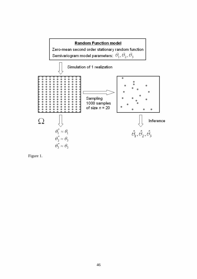
Figure 1 shows the design of the experiment for comparing methods for inferring

semivariogram parameters and the associated assessment of uncertainty. The underlying

random function (RF) model is a zero-mean, second-order, stationary function with a

given semivariogram model defined by a functional form (spherical, exponential or

Gaussian) and the semivariogram model parameters θ . A realization of the RF is

generated using any of the many methods available for non-conditional geostatistical

simulation (Chilès and Delfiner, 2012). Because the simulation is generated on a grid

defined on a finite region (Figure 1), there is an ergodic fluctuation in the simulation

(Deutsch and Journel, 1998) in the sense that, if the parameters are estimated from the

simulation, the semivariogram parameters *θ of a realization, may differ from the

underlying theoretical values θ . If many realizations of the RF are generated, then for

any sound geostatistical simulation method:

θθ }{E * (21)

For the purposes of this paper a single realisation is sufficient. The complete realisation

is a reality on the scale of the simulation grid and the complete realisation is such that

θθ * (22)

We can now sample this realisation using the number of samples that typifies a small

data set. The problem is to infer the underlying parameters θ from the small sample set.

15

To do so, we are seeking efficient inference methods that are able to give estimates

close to the underlying values θ and provide efficient measures of uncertainty in a

sense that we define later.

The factors that have the most significant influence on the outcomes of the experiment

are:

The sample size.

Whether of not the RF is Gaussian.

The nugget/variance ratio.

The ratio of the practical range to the characteristic length of the study area. The

characteristic length of the study area is a measure of the size of the simulation

region . If this region is a square, the characteristic length is the length of the

side of the square.

We use four simulated fields:

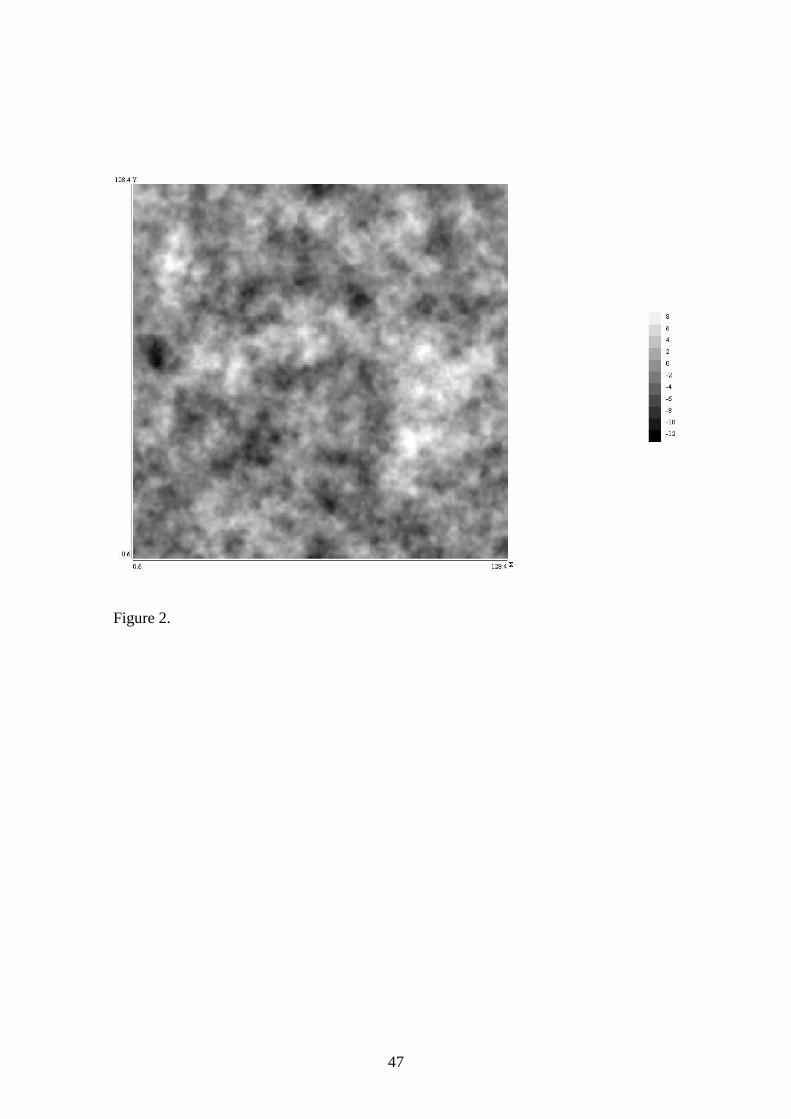
(A.) Gaussian field with no nugget variance, shown in Figure 2A.

(B.) Gaussian field with nugget variance equal to 50% of the total variance, shown

in Figure 2B.

(C.) Non-Gaussian random field with no nugget variance, shown in Figure 2C.

(D.) Non-Gaussian random field with nugget variance equal to 50% of the total

variance, shown in Figure 2D.

Each field is simulated on a 101×101 grid of points with unit distance between points

along the X and Y axes.

For each of the four fields we consider practical range/characteristic length ratios of 0.2

(Small), 0.4 (Medium) and 0.6 (Large). This gives twelve cases (four fields and three

16

ratios for each) and for each case we use sample sizes of 10, 30, 50, 70 and 90. For each

sample size we sample the field 1000 times to give 1000 data sets. Although we do not

use all these data files, we provide them as a benchmark data set for further comparisons

by others. The files are available on the usual site for software and supplementary

material for papers published in Computers & Geosciences at the www.iamg.org web

page. The semivariogram model is exponential with variance 10 units and range 6 units

(practical range 18 units of length). In cases B and D the nugget variance is 5, that is

50% of the total variance. The particular values of 6, 10 and 5 have no influence on the

results.

The non-Gaussian RF is a chi-squared random field with one degree of freedom (Pardo-

Igúzquiza and Dowd, 2005). Although the chi-squared RF is obtained by squaring a

Gaussian RF, it is not possible to recover the original Guassian field by a transformation

of the chi-squared RF, and in this sense, this represents a difficult case and a very good

example of non-Gaussian RF.

2.4. Criteria for the evaluations

Sampling consists of selecting the locations of the n data for each sample at random

from the grid locations of the complete realisation (Figure 1). For each sample, each

inference procedure provides a set of estimates θ and associated uncertainty measures

)ˆ(θU , which, for the general case, is the variance-covariance matrix of the estimates

)ˆ( Cθ U or a confidence region such as that given in Equation (19). Provided a

distribution is assumed for the estimates, the variance-covariance matrix can be used to

construct confidence regions for the set of estimates. We are interested in comparing

two performance measures for the inference methods: how well they estimate the

http://www.iamg.org/

17

underlying semivariogram parameters θ and the ability of the uncertainty measures to

evaluate the true uncertainty.

2.4. 1. Methods of evaluating estimators

The most common measure of the performance of the estimators is the mean square

error (MSE) defined as:

)ˆvar()ˆ(MSE Tθbbθ (23)

i.e., the square of the bias plus the variance, where the bias is given by

θθb (24)

}ˆE{θθ (25)

and the variance is:

})ˆ)(ˆ{(E)ˆvar( Tθθθθθ (26)

The MSE provides a measure of the closeness of the estimates to the true underlying

parameters. The square root of the mean square error (RMSE) is also used. As the

sampling distribution of the estimator is obtained for each parameter (Figure 1), other

measures of performance could also be obtained.

2.4. 2. Methods of evaluating uncertainty measures

An uncertainty measured is assigned to each estimate. The larger the uncertainty the less

will be the reliability of the estimate. One way of comparing uncertainty measures is by

using interval estimates constructed from the uncertainty measures. The two measures

for the intervals are size and coverage probability. The ideal is the narrowest interval

with the maximum possible coverage. There is a trade-off between size and coverage

because, usually, larger intervals have larger coverage. However, very large intervals,

even with large coverage, are of little use; for example, for a single parameter, the

18

interval ),( has a coverage of one, but it is obviously meaningless. For a single

parameter, the size of the confidence set is a length but, in the general case, it is a

volume of a multiple parameters. As there are many confidence sets with the same

probability coverage, we use the narrowest interval with the highest probability

coverage. In addition, the estimate must be inside the confidence set.

3. Results

For an underlying Gaussian random function, Pardo-Igúzquiza (1988) shows that ML

performs better than OLS, WLS or MLCV. Although we note that GLS and CV with

orthonormal residuals were not used in this comparison.

For the results reported here we used 100 samples for each estimator although we have

provided the files with 1000 data sets for each of the 40 cases. We show the results for

the worst case scenario. That is, the underlying RF model is non-Gaussian and there is

no possibility of transforming the data prior to applying the estimator or of correcting

the estimates. We use a practical range/field length ratio of 0.4 and compare the

estimators:

OLS: ordinary least squares using the complete semivariogram cloud.

WLS: weighted least squares, using the semivariogram cloud for distances less than 30

units); this is done by applying zero weights to the semivariogram cloud for distances

greater than 30 units.

WLS2: weighted least squares with binning.

GLS: generalized least squares with binning.

ML: maximum likelihood.

CV1: cross-validation

19

MLCV1: cross-validation with a global measure, i.e. maximum likelihood cross-

validation.

CV2: cross-validation with orthonormal residuals.

MLCV2: MLCV with orthonormal residuals.

4. Discussion

4.1. Estimation of semivariogram model parameters

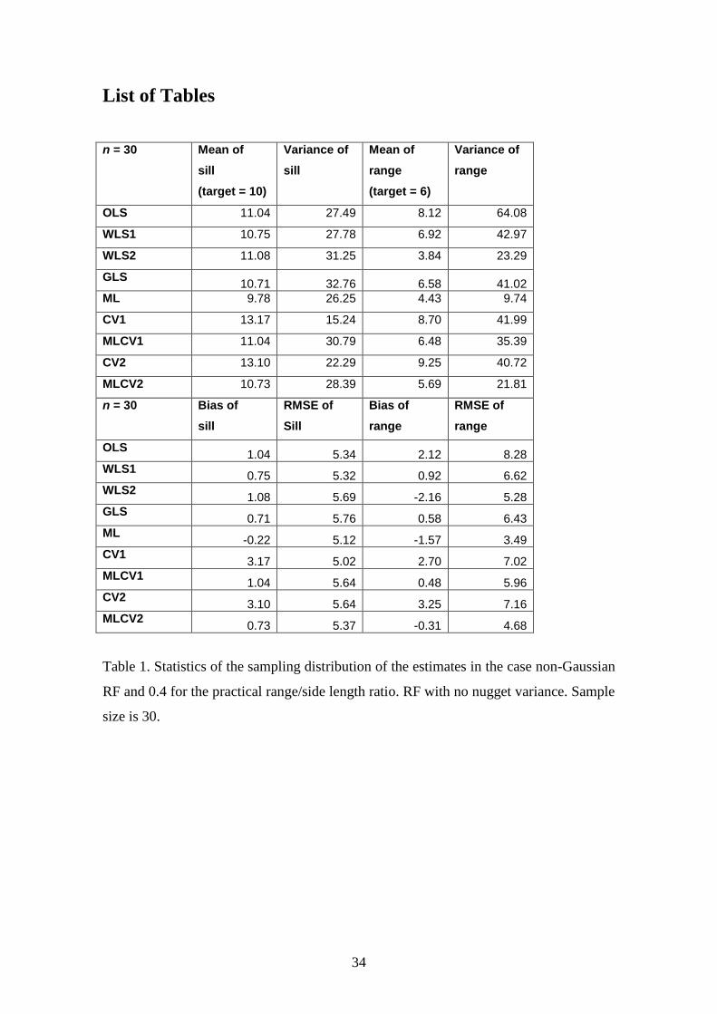
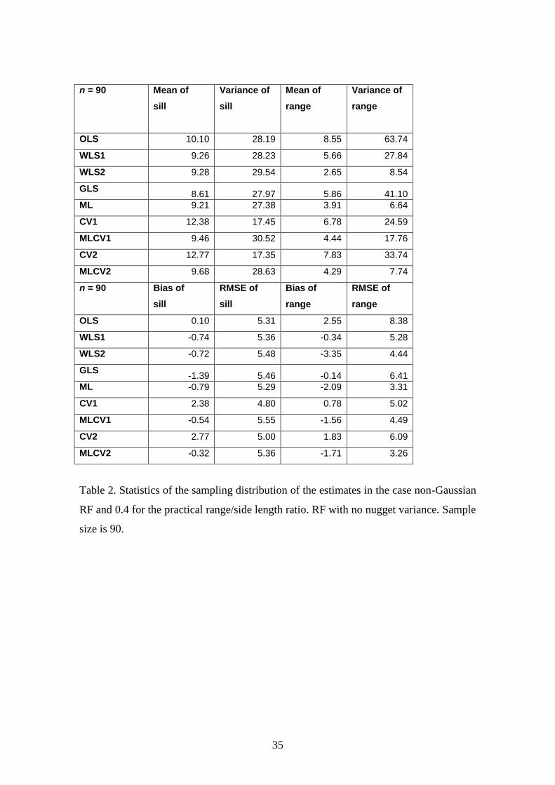
4.1.1. Non-Gaussian RF with no nugget variance

In this case there are two parameters to estimate, the range and the variance (sill). The

results are shown in Table 1 for a sample size of 30 and in Table 2 for a sample size of

90.

The conclusions for the range are:

The best estimator (in the sense of minimum RMSE) is ML for a sample size of

30 and MLCV2 for a sample size of 90 (although ML is second and close to

MLCV2).

The ML methods have a negative bias.

Among the LS estimators GLS is the best followed by WLS2.

There is no information lost in binning as GLS and WLS2 perform better than

methods that use the semivariogram cloud (OLS and WLS1).

WLS1 performs better than OLS, thus it is better not to use the semivariogram

values for long distances (high uncertainty).

CV methods are improved by including the global measure of overall accuracy,

i.e. converting them to MLCV methods.

Orthonormal residuals provide better results than ordinary residuals.

Conclusions for the sill:

20

All methods have very similar RMSE.

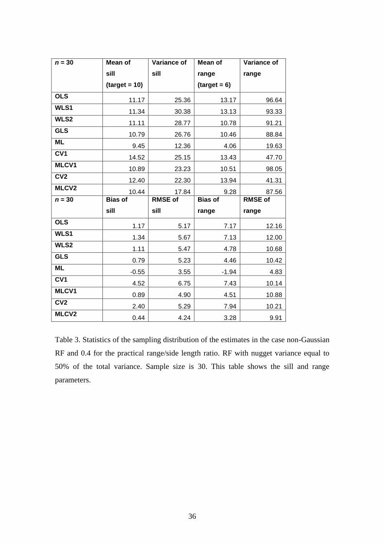
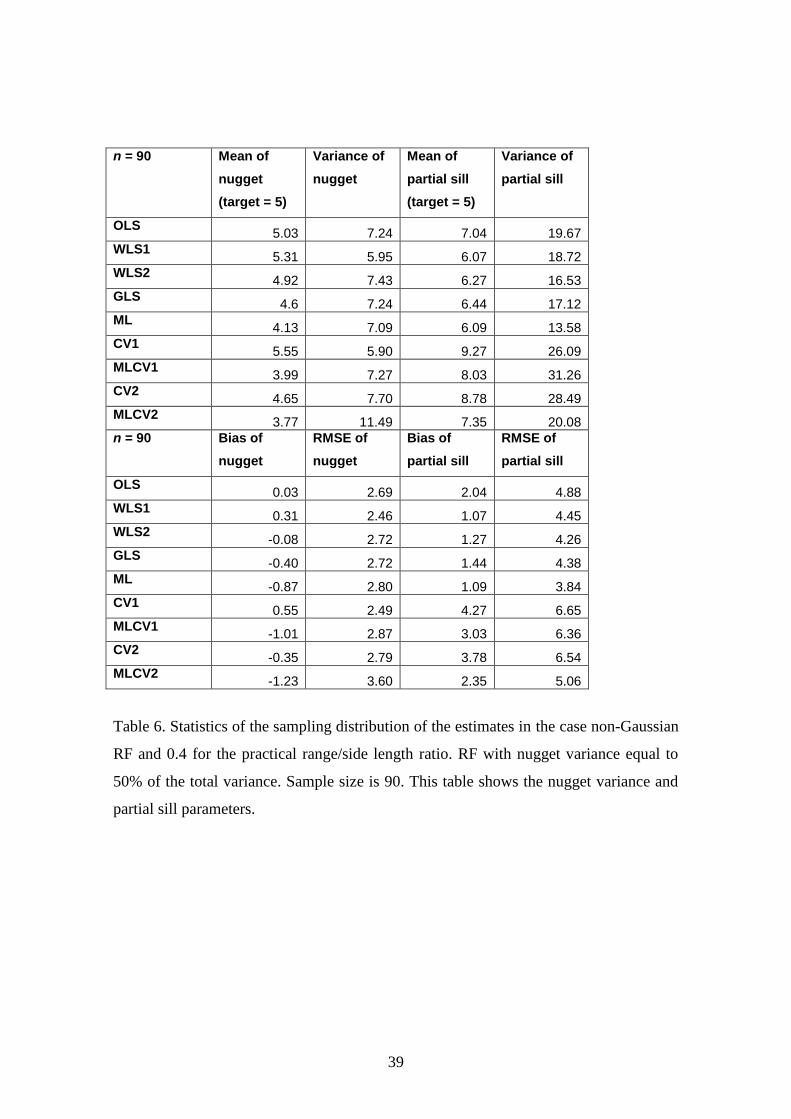
4.1.2. Non-Gaussian RF with nugget variance

In this case there are three parameters to estimate, the nugget variance, the partial sill

and range. The variance (total sill) is estimated as the sum of nugget variance and partial

sill. The results are shown in Tables 3 and 4 for a sample size of 30. Table 3 shows the

results for the sill and range parameters and Table 4 shows the results for nugget

variance and partial sill parameters. Tables 5 and 6 show the results for a sample size of

90. Table 5 shows the results for the sill and range parameters and Table 6 shows the

results for nugget variance and partial sill parameters.

Conclusions for the range:

The best estimator (in the sense of minimum RMSE) is ML for a sample size of

30 followed closely by GLS. The remaining methods have significantly higher

RMSE.

ML has a negative bias.

There is no information lost in binning as GLS and WLS2 perform better than

methods that use the semivariogram cloud (OLS and WLS1).

Orthonormal residuals provide better results than ordinary residuals but the

difference is less than when there is no nugget.

The RMSE is higher than for the case with no nugget (Table 1) and for all the

estimators. That is, the presence of noise in the model increases the noise in the

estimates and increases the uncertainty of the estimators.

Conclusions for the variance (total sill):

The RMSE is similar for all estimators and similar to the no nugget case except

for the GLS, which performs poorly.

21

Conclusions for the nugget variance:

CV1 gives the smallest RMSE. The other methods have similar performances

except GLS, which is the worst performer.

Conclusions for the partial sill:

ML gives the smallest RMSE. The other methods have similar performances.

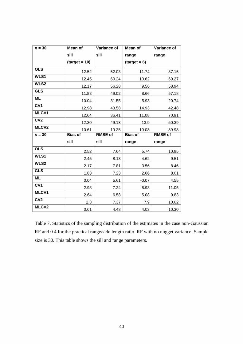
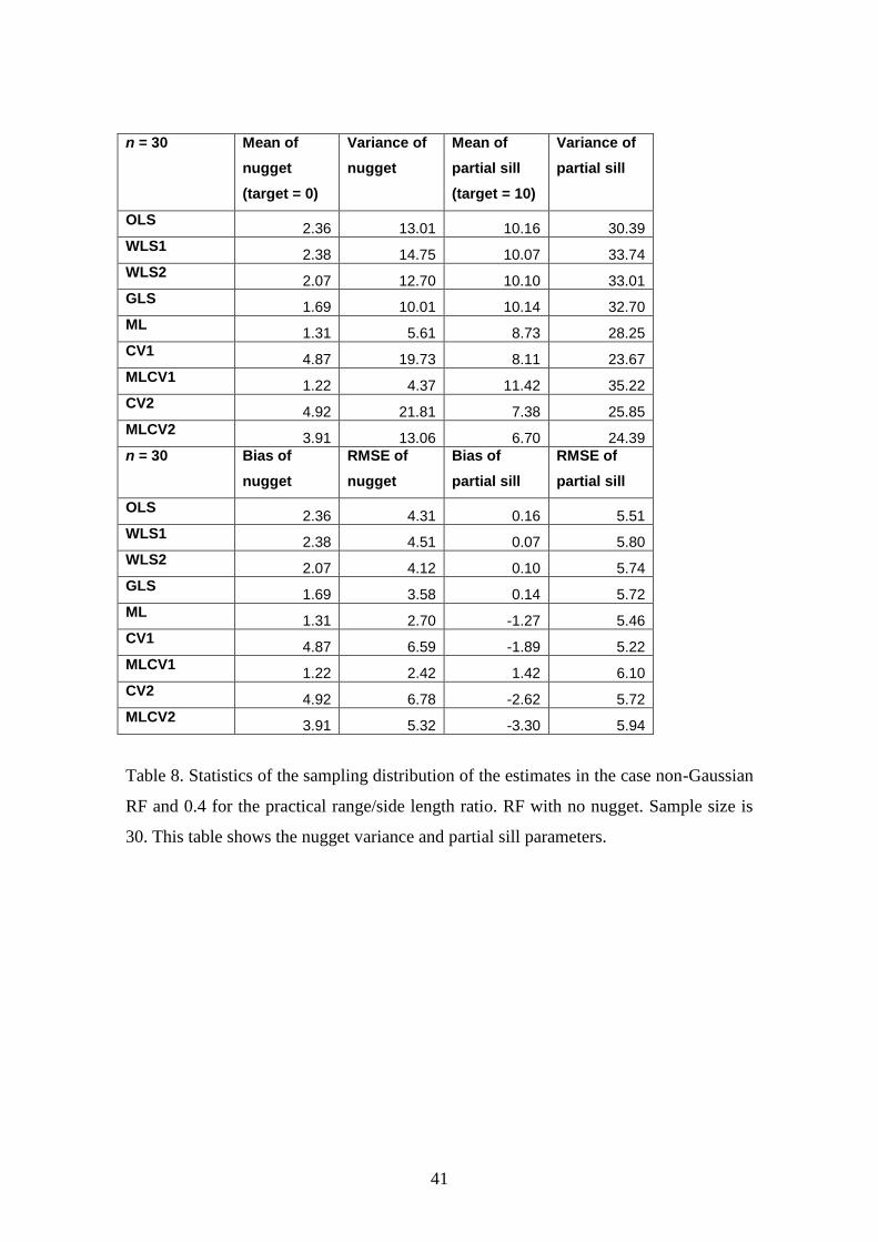
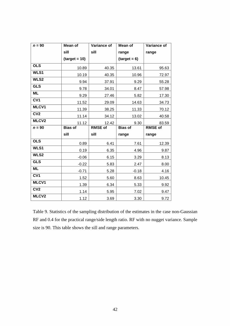
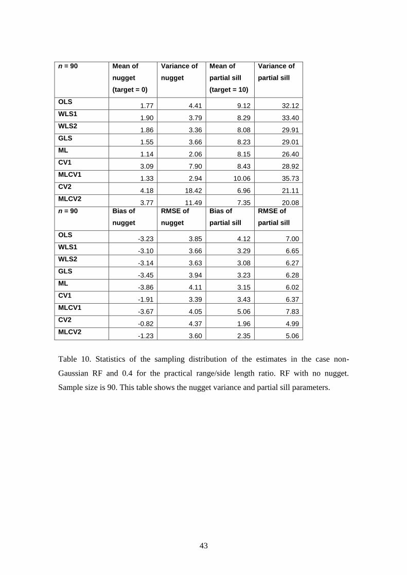
4.1.3. Non-Gaussian RF with estimated zero nugget variance

This example shows the consequence of estimating the nugget variance to be zero when

in fact the RF has no nugget.

The results are shown in Tables 7 and 8 for a sample size of 30. Table 7 shows the

results for the sill and range parameters and Table 8 shows the results for nugget

variance and partial sill parameters. Tables 9 and 10 show the results for a sample of

size 90. Table 9 shows the results for the sill and range parameters and Table 10 shows

the results for nugget variance and partial sill parameters.

Conclusions for the range:

The RMSE increases for all the methods. Thus if, from physical principles or

expert knowledge, it is known that there is no nugget variance then it is better

not to include the parameter in the estimation process.

ML is the best performer in the sense that its RMSE is a little higher than when

the nugget parameter is not included in the inference while the RMSE for other

estimators, including MLCV2, is double the value achieved when the nugget

parameter is not included in the inference.

Conclusions for the variance:

The RMSE for all methods except MLCV2 is increased but the increase in

RMSE for ML is the smallest.

Conclusions for the nugget variance:

22

All methods estimate a nugget greater than zero. The smallest bias (i.e. value

closest to zero) is for ML for n = 30 and MLCV1 for n = 90.

Conclusions for the partial sill:

The partial sill, which is equal to the sill or total variance because the nugget

variance of the RF is zero, is estimated with smaller RMSE than the variance

because the variance is estimated as the sum of partial sill and nugget variance.

4.2. Joint estimation of several parameters

In order to evaluate the performance of the methods, the RMSE is accumulated and the

methods are ranked according to their scores. The results are shown in Table 11. In

increasing order of total RMSE, the ranked methods are: ML (259), MLCV2 (340),

WLS2 (357), GLS (366), MLCV1 (370), WLS1 (379), CV1 (389), CV2 (396), OLS

(416). For the range the best is ML (26) with almost half the RMSE of any other

method. MLCV2 is second (48). For the nugget variance, ML (11) and MLCV1 (11) are

the best. For the partial sill ML is the best (19) closely followed by three methods (21).

Finally, for the variance (sill) MLCV2 is the best (27) closely followed by ML (28).

4.3. Assessment of the uncertainty of the estimates

We can compare the uncertainty evaluations by comparing the coverage and the width

of the intervals. However, it should be borne in mind that we have chosen to use the

worst-case scenario in which the RF is highly non-Gaussian, there is no transformation

of the data and no transformation of the estimates. On the other hand all the uncertainty

evaluations are parametric with Gaussian or chi-square distribution assumptions for the

given statistics, i.e., Equations (14), (15), (18) and (19).

23

By way of example, the results of Equations (14) and (15) for GLS and ML are given in

Table 12. Because the assumptions are not correct there is no correspondence between

the actual coverage and the nominal coverage under the Gaussian assumption. This

requires further work, for example, implementing non-parametric approaches like a

bootstrap procedure.

5. Conclusions

The primary purpose of this paper is to compare methods of inferring semivariogram

model parameters. The study is limited to small samples from a two-dimensional,

second-order stationary non-Gaussian random function with an isotropic semivariogram

model with and without a nugget effect.

The OLS estimator using the full semivariogram cloud is the worst performer among

the set of estimators that have been compared. The estimator may be improved in two

ways: (1) by using WLS1 with zero weights applied to those data pairs in the

semivariogram cloud that are separated by significant distances. Uncertainty of the

semivariogram values increases with distance and beyond a certain limit there is no

value in including them in the estimator; (2) by using WLS2 and using only

semivariogram lags up to a given distance (for example one third of the study area or

three times the expected range). GLS gives similar results to WLS2. This may be

because we have used the worst-case scenario with a highly skewed non-Gaussian RF

from which the original distribution cannot be recovered.

Among the cross-validation estimators those that use the global measure of accuracy of

Kitanidis (1991) have proved superior to the others. Estimators that use the global

measure are equivalent to the maximum likelihood cross-validation method. In addition,

24

the orthonormal residuals give better results than classical residuals. Thus MLCV2 is

the best among the cross-validation estimators and the second best among all the

estimators tested.

ML is the best estimator even when the data are non-Gaussian. ML is a good measure of

the goodness of fit of a semivariogram model to the experimental data.

If there is no reason to believe that a nugget variance is present in the data, the results

can be improved by not including this parameter in the inference, i.e., implicitly taking

it to be zero.

Finally, further research is needed on the estimation of uncertainty measures with a

given probabilistic coverage in the worst-case scenario.

Acknowledgements

This work was supported by research projects CGL2010-15498 and CGL2010-17629

from the Ministerio de Economia y Competitividad of Spain and by the Australian

Research Council through Discovery Project grant DP110104766.

List of acronyms

RF: random function.

OLS: ordinary least squares with the complete semivariogram cloud.

WLS1: weighted least squares with the semivariogram cloud for distances less than a

distance threshold.

WLS2: weighted least squares with binned semivariogram data.

GLS: generalized least squares with binned semivariogram data.

ML: maximum likelihood.

CV1: cross-validation.

CV2: cross-validation with orthonormal residuals.

25

MLCV1: maximum likelihood cross-validation.

MLCV2: maximum likelihood cross-validation with orthonormal residuals.

RMSE: root mean square error.

References

Bard, Y., 1974. Nonlinear parameter estimation. John Wiley and Sons, New York, 341

p.

Bogaert, P., Russo, D., 1999. Optimal spatial sampling design for he estimation of the

variogram based on a least squares approach. Water Resources Research, 35 (4),

1275-1289.

Burrough, P.A., 2001. GIS and geostatistics: Essential partners for spatial analysis.

Environmental and Ecological Statistics 8, 361-377.

Caers, J., 2005. Petroleum Geostatistics. Society of Petroleum Engineers, Richardson,

TX, 88 p.

Chica-Olmo, M., Abarca-Hernández, F., 2000. Computing geostatistical image textura

for remotely sensed data classification. Computers & Geosciences 26, 373-383.

Chilès, J.P., Delfiner, P., 2012. Geostatistics. Modeling Spatial Uncertainty. Second

Edition. John Wiley & Sons, Hoboken, New Jersey, 702 p.

Cressie, N., 1985. Fitting variogram models by weighted least squares. Mathematical

Geology 17 (5), 563-586.

Curran, P.J., Atkinson, P.M., 1998. Geostatistics and remote sensing. Progress in

Physical Geography 22 (1), 61-78.

26

Deutsch, C.V. 2002. Geostatistical reservoir modeling. Oxford University Press, New

York, 384 p

Deutsch, C.V., Journel, A.G., 1998. GSLIB. Geostatistical Software Library and User´s

Guide. Second Edition. Oxford University Press, 384 p.

Diggle, P.J., Ribeiro Jr, P.J., 2007. Model Based Geostatistics. Springer-Verlag , New

York, 228 p.

Diodato, N., Ceccarelli, M., 2005. Interpolation processes using multivariate

geostatistics for mapping of climatological precipitation mean in the Sannio

Mountains (southern Italy). Earth Surface Processes and Landforms 30 (3), 259-

268.

Dowd, P.A. (1983) The variogram and kriging: robust and resistant estimators. in Verly,

G. et. al. (eds.) Geostatistics for Natural Resource Characterization Part 1;

NATO A.S.I. Series C: Mathematical and Physical Sciences, volume 122, pub.

D. Reidel Publishing Co., Dordrecht, Netherlands, 91-106.

Genton, M.G., 1998. Highly robust variogram estimation. Mathematical Geology 30

(2), 213-221.

Griffith, D.A., Paelinck, J.H.P., 2011. Non-standard Spatial Statistics and Spatial

Econometrics, Springer, Berlin, 262 p.

Goovaerts, P., 1997. Geostatistics for Natural Resources Evaluation. Oxford University

Press, New York, 463 p.

Gringarten, E., Deutsch, C.V., 2001. Teacher’s Aide Variogram Interpretation and

Modeling 33 (4), 507-534.

Journel, A.G., Rossi, M.E., 1989. When do we need a trend model in kriging.

Mathematical Geology 21 (7), 715-739.

27

Kalbfleisch, J.G., 1979. Probability and Statistical Inference II. New York, Springer-

Verlag.

Kelsall, J., Wakefield J., 2002. Modeling spatial variation in disease risk: a

geostatistical approach. Journal of the Americal Statistical Association 97 (459),

692-701.

Kitanidis, P.K., 1983. Statistical estimation of polynomial generalized covariance

functions and hydrologic applications. Water Resources Research 19 (4), 909-

921.

Kitanidis, P.K., 1991. Orthonomal residuals in geostatistics: model criticism and

parameter estimation. Mathematical Geology 23 (5), 741-757.

Kitanidis, P.K., 1997. Introduction to Geostatistics. Applications to Hydrogeology.

Cambridge University Press, Cambridge, 249 p.

Kitanidis, P.K., Lane R.W., 1985. Maximum likelihood parameter estimation of

hydrologic spatial processes by the Gaussian-Newton method. Journal of

Hydrology 79 (1-2), 53-71.

Krajewski, W.F., Duffy C.J., 1988. Estimation of correlation structure for a

homogeneous isotropic random field: a simulation study. Computers &

Geosciences 14 (1), 113-122.

Lebel T., Bastin G., 1985. Variogram identification by mean squared interpolation error

method with application to hydrologic fields. Journal of Hydrology 77 (1-4), 31-

56.

Liebhold, A.M., Rossi, R.E., Kemp, W.P., 1993. Geostatistics and Geographic

Information Systems in Applied Insect Ecology. Annual Review of Entomology

38, 303-327.

28

Mardia, K.V., Marshall, R.J., 1984. Maximum likelihood estimation of models for

residual covariance in spatial regression. Biometrika 71 (1), 135-146.

Matheron, G., 1963. Principles of Geostatistics. Economic Geology 58, 1246-1266.

Menke, W., 1984, Geophysical data analysis: Discrete inverse theory: Academic Press,

San Diego, CA, 285 p.

McCullagh, P., Nelder, J.A., 1989. Generalized Linear Models, 2nd ed. Cambridge,

Massachusetts, Chapman and Hall.

O’Brien, J.J., Griffiths, J.F., 1965. The rank correlation coefficient as an indicator of the

product-moment correlation coefficient for small samples (10-100). Journal of

Geophysical Research 70 (8): 1995-1998.

Olea, R., Pardo-Igúzquiza, E., 2011. Generalizad bootstrap method for assessing of

uncertainty in semivariogram inference. Mathematical geosciences 43 (2), 203-

228.

Pardo-Igúzquiza, E., 1998. Maximum likelihood estimation of spatial covariance

parameters. Mathematical Geology 30 (1), 95-108.

Pardo-Igúzquiza, E., 1999a. Bayesian inference of spatial covariance parameters.

Mathematical Geology 31 (1), 47-65.

Pardo-Igúzquiza, E., 1999b. VARFIT: a fortran-77 program for fitting variogram

models by weighted least squares. Computer & Geosciences 25 (3), 251-261.

Pardo-Igúzquiza E., Chica-Olmo M., Luque-Espinar, J. A., and García-Soldado, M.J.,

2009. Using semivariogram parameter uncertainty in hydrogeological

applications. Groundwater, 47 (1), 25-34

Pardo-Igúzquiza, E. Dowd, P.A., 2001. Variance-covariance matrix of the experimental

variogram: assessing variogram uncertainty. Mathematical Geology,33 (4), 397-

419.

29

Pardo-Igúzquiza, E. and Dowd, P.A., 2003. Assessment of the uncertainty of spatial

covariance parameters of soil properties and its use in applications. Soil Science

168 (11): 769-782.

Pardo-Igúzquiza, E., Dowd, P.A., 2005. Empirical maximum likelihood kriging: the

general case. Mathematical Geology. v. 37, no 5, pp. 477-492

Rice, J.A., 1995. Mathematical Statistics and Data Analysis. Second Edition, Duxbury

Press, Belmont, California, 602 p.

Russo, D., Jury W.A., 1987. A theoretical study of the estimation of the correlation

scale in spatially variable fields: 1. Stationary fields. Water Resources Research

23 (7), 1257-1268.

Samper, F.J., Neuman S.P., 1989. Estimation of spatial covariance structures by adjoint

state maximum likelihood cross-validation: 1. Theory. Water Resources

Research 25 (3), 351-362.

Sampson, P.D., Guttorp P., 1992. Nonparametric estimation of nonstationay spatial

covariance structure. Journal of the Americal Statistical Association 87 (417),

108-119.

Solow, A.R., 1985. Bootstrapping correlated data. Mathematical Geology 17 (7), 769-

775

Spiegel, M.R., Stephens L.J., 2008. Statistics. Forth Edition, McGraw-Hill Professional,

New York, 577 p.

Strebelle, S., 2002. Conditional simulation of complex geological structures using

multiple-point statistics. Mathematical Geology 34, 1-22.

Visser, A., Dubus I., Broers H.P., Brouyère S., Korcz M., Orban P., Goderniaux P.,

Batlle-Aguilar J., Surdyk N. Amraoui N., Job H., Pinault J.L., Bierkens M.,

30

2009. Comparison of methods for the detection and extrapolation of trends in

groundwater quality. Journal of Environmental Monitoring 11, 2030-2043.

Ye, M., Meyer P.D., Neuman, S.P., 2008. On model selection criteria in multimodel

analysis. Water Resources Research 44, W03428, 1-12.

Zimmerman, D.L., Zimmerman, M.B., 1991. A comparison of spatial semivariogram

estimators and corresponding ordinary kriging predictors. Technometrics 33 (1),

77-91.

List of Tables

Table 1. Statistics of the sampling distribution of the estimates for a non-Gaussian RF

and a practical range/side length ratio of 0.4. RF with no nugget variance. Sample size

is 30.



is 90.


and a practical range/side length ratio of 0.4. RF with nugget variance equal to 50% of

the total variance. Sample size is 30. This table shows the sill and range parameters.



31

the total variance. Sample size is 30. This Table shows the nugget variance and partial

sill parameters.



the total variance. Sample size is 90. This Table shows the sill and range parameters.

List of Figures

Figure 1. Design of the experiment for selecting small sample sets on which to compare

estimators.

Figure 2. A: Realization of a zero-mean Gaussian field with exponential semivariogram

with range 6 units (practical range 18 units of distance). The nugget variance is zero and

the variance is 10. B: Realization of a zero-mean Gaussian field with exponential

semivariogram with range 6 units (practical range 18 units of distance). The nugget

variance is 50% of the total variance. The total variance is 10, the nugget variance is 5

and the partial sill is 5. C: Realization of a chi-square field with exponential

semivariogram with range 6 units (practical range 18 units of distance). The nugget

variance is zero and the total variance is 10. D: Realization of a chi-square field with

exponential semivariogram with range 6 units (practical range 18 units of distance). The

nugget variance is 50% of the total variance. The variance is 10, the nugget variance is 5

and the partial sill is 5.

32



is 30.



is 90.



the total variance. Sample size is 30. This table shows the sill and range parameters.




sill parameters.



the total variance. Sample size is 90. This Table shows the sill and range parameters.




sill parameters.

33



is 30. This Table shows the sill and range parameters.


and a practical range/side length ratio of 0.4. RF with no nugget. Sample size is 30. This

Table shows the nugget variance and partial sill parameters.



is 90. This Table shows the sill and range parameters.


and a practical range/side length ratio of 0.4. RF with no nugget. Sample size is 90.

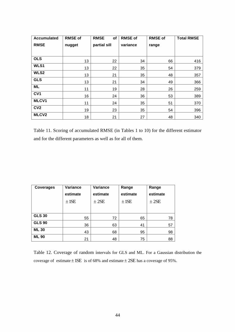
Table 11. Scoring of accumulated RMSE (in Tables 1 to 10) of the estimators for each

parameter and for the total model.

Table 12. Coverage of random intervals for GLS and ML. For a Gaussian distribution

the coverage of estimate SE1 is of 68% and estimate SE2 has a coverage of 95%.

34

List of Tables

n = 30 Mean of

sill

(target = 10)

Variance of

sill

Mean of

range

(target = 6)

Variance of

range

OLS 11.04 27.49 8.12 64.08

WLS1 10.75 27.78 6.92 42.97

WLS2 11.08 31.25 3.84 23.29

GLS 10.71 32.76 6.58 41.02

ML 9.78 26.25 4.43 9.74

CV1 13.17 15.24 8.70 41.99

MLCV1 11.04 30.79 6.48 35.39

CV2 13.10 22.29 9.25 40.72

MLCV2 10.73 28.39 5.69 21.81

n = 30 Bias of

sill

RMSE of

Sill

Bias of

range

RMSE of

range

OLS 1.04 5.34 2.12 8.28

WLS1 0.75 5.32 0.92 6.62

WLS2 1.08 5.69 -2.16 5.28

GLS 0.71 5.76 0.58 6.43

ML -0.22 5.12 -1.57 3.49

CV1 3.17 5.02 2.70 7.02

MLCV1 1.04 5.64 0.48 5.96

CV2 3.10 5.64 3.25 7.16

MLCV2 0.73 5.37 -0.31 4.68

Table 1. Statistics of the sampling distribution of the estimates in the case non-Gaussian

RF and 0.4 for the practical range/side length ratio. RF with no nugget variance. Sample

size is 30.

35

n = 90 Mean of

sill

Variance of

sill

Mean of

range

Variance of

range

OLS 10.10 28.19 8.55 63.74

WLS1 9.26 28.23 5.66 27.84

WLS2 9.28 29.54 2.65 8.54

GLS 8.61 27.97 5.86 41.10

ML 9.21 27.38 3.91 6.64

CV1 12.38 17.45 6.78 24.59

MLCV1 9.46 30.52 4.44 17.76

CV2 12.77 17.35 7.83 33.74

MLCV2 9.68 28.63 4.29 7.74

n = 90 Bias of

sill

RMSE of

sill

Bias of

range

RMSE of

range

OLS 0.10 5.31 2.55 8.38

WLS1 -0.74 5.36 -0.34 5.28

WLS2 -0.72 5.48 -3.35 4.44

GLS -1.39 5.46 -0.14 6.41

ML -0.79 5.29 -2.09 3.31

CV1 2.38 4.80 0.78 5.02

MLCV1 -0.54 5.55 -1.56 4.49

CV2 2.77 5.00 1.83 6.09

MLCV2 -0.32 5.36 -1.71 3.26



size is 90.

36

n = 30 Mean of

sill

(target = 10)

Variance of

sill

Mean of

range

(target = 6)

Variance of

range

OLS 11.17 25.36 13.17 96.64

WLS1 11.34 30.38 13.13 93.33

WLS2 11.11 28.77 10.78 91.21

GLS 10.79 26.76 10.46 88.84

ML 9.45 12.36 4.06 19.63

CV1 14.52 25.15 13.43 47.70

MLCV1 10.89 23.23 10.51 98.05

CV2 12.40 22.30 13.94 41.31

MLCV2 10.44 17.84 9.28 87.56

n = 30 Bias of

sill

RMSE of

sill

Bias of

range

RMSE of

range

OLS 1.17 5.17 7.17 12.16

WLS1 1.34 5.67 7.13 12.00

WLS2 1.11 5.47 4.78 10.68

GLS 0.79 5.23 4.46 10.42

ML -0.55 3.55 -1.94 4.83

CV1 4.52 6.75 7.43 10.14

MLCV1 0.89 4.90 4.51 10.88

CV2 2.40 5.29 7.94 10.21

MLCV2 0.44 4.24 3.28 9.91


RF and 0.4 for the practical range/side length ratio. RF with nugget variance equal to

50% of the total variance. Sample size is 30. This table shows the sill and range

parameters.

37

n = 30 Mean of

nugget

(target = 5)

Variance of

nugget

Mean of

partial sill

(target = 5)

Variance of

partial sill

OLS 4.32 10.93 6.85 27.72

WLS1 4.51 12.37 6.83 28.52

WLS2 4.38 15.67 6.73 27.37

GLS 3.91 13.08 6.88 25.86

ML 3.87 10.71 5.58 20.88

CV1 4.93 7.70 9.59 25.64

MLCV1 4.23 12.15 6.66 30.08

CV2 4.51 11.51 7.89 24.15

MLCV2 4.40 11.08 6.04 23.13

n = 30 Bias of

nugget

RMSE of

nugget

Bias of

partial sill

RMSE of

partial sill

OLS -0.68 3.37 1.85 5.58

WLS1 -0.49 3.55 1.83 5.64

WLS2 -0.62 4.00 1.73 5.51

GLS -1.09 3.77 1.88 5.42

ML -1.13 3.46 0.58 4.60

CV1 -0.07 2.77 4.59 6.83

MLCV1 -0.77 3.57 1.66 5.73

CV2 -0.49 3.42 2.89 5.70

MLCV2 -0.60 3.38 1.04 4.92



50% of the total variance. Sample size is 30. This table shows the nugget variance and

partial sill parameters.

38

n = 90 Mean of

sill

(target = 10)

Variance of

sill

Mean of

range

(target = 6)

Variance of

range

OLS 12.07 15.26 15.82 86.02

WLS1 11.38 13.81 12.92 72.87

WLS2 11.19 13.91 11.34 81.90

GLS 11.04 14.79 9.68 81.23

ML 10.22 8.61 5.56 28.62

CV1 14.82 18.64 13.3 35.73

MLCV1 12.02 28.94 9.38 90.49

CV2 13.43 21.12 14.04 47.23

MLCV2 10.44 17.84 9.28 87.56

n = 90 Bias of

sill

RMSE of

sill

Bias of

range

RMSE of

range

OLS 2.07 4.42 9.82 13.50

WLS1 1.38 3.96 6.92 10.98

WLS2 1.19 3.91 5.34 10.50

GLS 1.04 3.98 3.68 9.73

ML 0.22 2.94 -0.44 5.36

CV1 4.82 6.47 7.30 9.43

MLCV1 2.02 5.74 3.38 10.09

CV2 3.43 5.73 8.04 10.57

MLCV2 1.12 3.69 3.30 9.72



50% of the total variance. Sample size is 90. This table shows the sill and range

parameters.

39

n = 90 Mean of

nugget

(target = 5)

Variance of

nugget

Mean of

partial sill

(target = 5)

Variance of

partial sill

OLS 5.03 7.24 7.04 19.67

WLS1 5.31 5.95 6.07 18.72

WLS2 4.92 7.43 6.27 16.53

GLS 4.6 7.24 6.44 17.12

ML 4.13 7.09 6.09 13.58

CV1 5.55 5.90 9.27 26.09

MLCV1 3.99 7.27 8.03 31.26

CV2 4.65 7.70 8.78 28.49

MLCV2 3.77 11.49 7.35 20.08

n = 90 Bias of

nugget

RMSE of

nugget

Bias of

partial sill

RMSE of

partial sill

OLS 0.03 2.69 2.04 4.88

WLS1 0.31 2.46 1.07 4.45

WLS2 -0.08 2.72 1.27 4.26

GLS -0.40 2.72 1.44 4.38

ML -0.87 2.80 1.09 3.84

CV1 0.55 2.49 4.27 6.65

MLCV1 -1.01 2.87 3.03 6.36

CV2 -0.35 2.79 3.78 6.54

MLCV2 -1.23 3.60 2.35 5.06



50% of the total variance. Sample size is 90. This table shows the nugget variance and

partial sill parameters.

40

n = 30 Mean of

sill

(target = 10)

Variance of

sill

Mean of

range

(target = 6)

Variance of

range

OLS 12.52 52.03 11.74 87.15

WLS1 12.45 60.24 10.62 69.27

WLS2 12.17 56.28 9.56 58.94

GLS 11.83 49.02 8.66 57.18

ML 10.04 31.55 5.93 20.74

CV1 12.98 43.58 14.93 42.48

MLCV1 12.64 36.41 11.08 70.91

CV2 12.30 49.13 13.9 50.39

MLCV2 10.61 19.25 10.03 89.98

n = 30 Bias of

sill

RMSE of

sill

Bias of

range

RMSE of

range

OLS 2.52 7.64 5.74 10.95

WLS1 2.45 8.13 4.62 9.51

WLS2 2.17 7.81 3.56 8.46

GLS 1.83 7.23 2.66 8.01

ML 0.04 5.61 -0.07 4.55

CV1 2.98 7.24 8.93 11.05

MLCV1 2.64 6.58 5.08 9.83

CV2 2.3 7.37 7.9 10.62

MLCV2 0.61 4.43 4.03 10.30



size is 30. This table shows the sill and range parameters.

41

n = 30 Mean of

nugget

(target = 0)

Variance of

nugget

Mean of

partial sill

(target = 10)

Variance of

partial sill

OLS 2.36 13.01 10.16 30.39

WLS1 2.38 14.75 10.07 33.74

WLS2 2.07 12.70 10.10 33.01

GLS 1.69 10.01 10.14 32.70

ML 1.31 5.61 8.73 28.25

CV1 4.87 19.73 8.11 23.67

MLCV1 1.22 4.37 11.42 35.22

CV2 4.92 21.81 7.38 25.85

MLCV2 3.91 13.06 6.70 24.39

n = 30 Bias of

nugget

RMSE of

nugget

Bias of

partial sill

RMSE of

partial sill

OLS 2.36 4.31 0.16 5.51

WLS1 2.38 4.51 0.07 5.80

WLS2 2.07 4.12 0.10 5.74

GLS 1.69 3.58 0.14 5.72

ML 1.31 2.70 -1.27 5.46

CV1 4.87 6.59 -1.89 5.22

MLCV1 1.22 2.42 1.42 6.10

CV2 4.92 6.78 -2.62 5.72

MLCV2 3.91 5.32 -3.30 5.94


RF and 0.4 for the practical range/side length ratio. RF with no nugget. Sample size is

30. This table shows the nugget variance and partial sill parameters.

42

n = 90 Mean of

sill

(target = 10)

Variance of

sill

Mean of

range

(target = 6)

Variance of

range

OLS 10.89 40.35 13.61 95.63

WLS1 10.19 40.35 10.96 72.97

WLS2 9.94 37.91 9.29 55.28

GLS 9.78 34.01 8.47 57.98

ML 9.29 27.46 5.82 17.30

CV1 11.52 29.09 14.63 34.73

MLCV1 11.39 38.25 11.33 70.12

CV2 11.14 34.12 13.02 40.58

MLCV2 11.12 12.42 9.30 83.59

n = 90 Bias of

sill

RMSE of

sill

Bias of

range

RMSE of

range

OLS 0.89 6.41 7.61 12.39

WLS1 0.19 6.35 4.96 9.87

WLS2 -0.06 6.15 3.29 8.13

GLS -0.22 5.83 2.47 8.00

ML -0.71 5.28 -0.18 4.16

CV1 1.52 5.60 8.63 10.45

MLCV1 1.39 6.34 5.33 9.92

CV2 1.14 5.95 7.02 9.47

MLCV2 1.12 3.69 3.30 9.72



size is 90. This table shows the sill and range parameters.

43

n = 90 Mean of

nugget

(target = 0)

Variance of

nugget

Mean of

partial sill

(target = 10)

Variance of

partial sill

OLS 1.77 4.41 9.12 32.12

WLS1 1.90 3.79 8.29 33.40

WLS2 1.86 3.36 8.08 29.91

GLS 1.55 3.66 8.23 29.01

ML 1.14 2.06 8.15 26.40

CV1 3.09 7.90 8.43 28.92

MLCV1 1.33 2.94 10.06 35.73

CV2 4.18 18.42 6.96 21.11

MLCV2 3.77 11.49 7.35 20.08

n = 90 Bias of

nugget

RMSE of

nugget

Bias of

partial sill

RMSE of

partial sill

OLS -3.23 3.85 4.12 7.00

WLS1 -3.10 3.66 3.29 6.65

WLS2 -3.14 3.63 3.08 6.27

GLS -3.45 3.94 3.23 6.28

ML -3.86 4.11 3.15 6.02

CV1 -1.91 3.39 3.43 6.37

MLCV1 -3.67 4.05 5.06 7.83

CV2 -0.82 4.37 1.96 4.99

MLCV2 -1.23 3.60 2.35 5.06

Table 10. Statistics of the sampling distribution of the estimates in the case non-

Gaussian RF and 0.4 for the practical range/side length ratio. RF with no nugget.

Sample size is 90. This table shows the nugget variance and partial sill parameters.

44

Accumulated

RMSE

RMSE of

nugget

RMSE of

partial sill

RMSE of

variance

RMSE of

range

Total RMSE

OLS 13 22 34 66 416

WLS1 13 22 35 54 379

WLS2 13 21 35 48 357

GLS 13 21 34 49 366

ML 11 19 28 26 259

CV1 16 24 36 53 389

MLCV1 11 24 35 51 370

CV2 19 23 35 54 396

MLCV2 18 21 27 48 340

Table 11. Scoring of accumulated RMSE (in Tables 1 to 10) for the different estimator

and for the different parameters as well as for all of them.

Coverages Variance

estimate

SE1

Variance

estimate

SE2

Range

estimate

SE1

Range

estimate

SE2

GLS 30 55 72 65 78

GLS 90 36 63 41 57

ML 30 43 68 95 98

ML 90 21 48 75 88

Table 12. Coverage of random intervals for GLS and ML. For a Gaussian distribution the

coverage of estimate SE1 is of 68% and estimate SE2 has a coverage of 95%.

45

List of Figures

Figure 1. Design of the experiment in order to have the small samples for comparing

estimators.

Figure 2. Realization of a zero-mean Gaussian field with exponential semi-variogram of

range 6 units (practical range 18 units of distance). The nugget variance is zero and the

variance is 10.

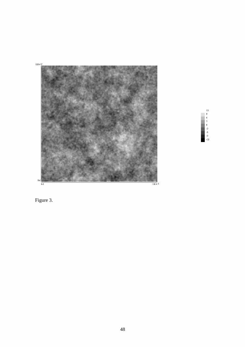
Figure 3. Realization of a zero-mean Gaussian field with exponential semi-variogram of

range 6 units (practical range 18 units of distance). The nugget variance is 50% of the

total variance. The total is 10, the nugget variance is 5 and the partial sill is 5.

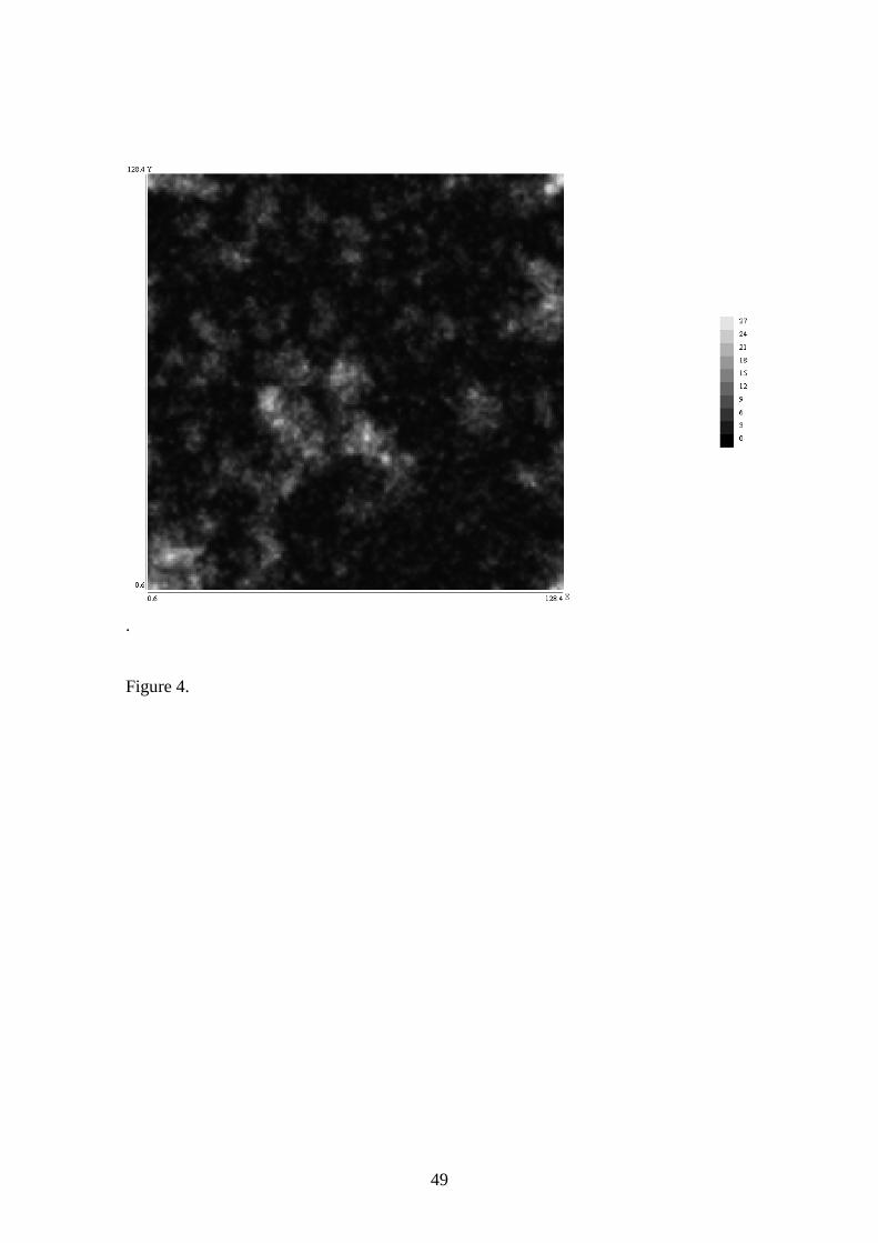
Figure 4. Realization of a chi-square field with exponential semi-variogram of range 6

units (practical range 18 units of distance). The nugget variance is zero and the variance

is 10.

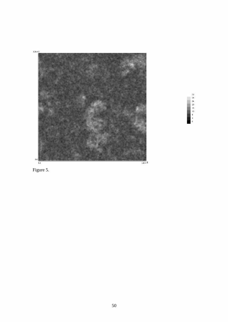
Figure 5. Realization of a chi-square field with exponential semi-variogram of range 6

units (practical range 18 units of distance). The nugget variance is 50% the total

variance. The variance is 10, the nugget variance is 5 and the partial sill is 5.

46

Figure 1.

47

Figure 2.

48

Figure 3.

49

.

Figure 4.

50

Figure 5.

Special issue computers & geosciences - CORE · PDF filesampling theory (Spiegel and Stephens,...

Documents

Transcript of Special issue computers & geosciences - CORE · PDF filesampling theory (Spiegel and Stephens,...