GRAD6/8104; INES 8090 Spatial Statistic Spring 2017

1

Lab #4 Semivariogram and Kriging (Due Date: 04/04/2017)

PURPOSES 1. Learn to conduct semivariogram analysis and kriging for geostatistical data 2. Learn to use a spatial statistical library, gstat, in R for inference on geostatistical data

Before starting your lab, create a new directory named lab4 in your network drive (where you could organize files for this course), and create a Word document named lab4_yourusername.doc for your lab write up.

A suite of geostatistical approaches exist to support inference for geostatistical data. We have learned semivariogram, covariance, and Kriging methods. In this lab, we will focus on learning to conduct semivariogram analysis and Kriging for spatial interpolation using a library in R: gstat. 1. Basics for the gstat package in R The gstat package is available from the following link: http://cran.r-project.org/web/packages/gstat/index.html First, install the gstat package (refer to lab1-3 for installation instruction as needed). The gstat package allows us to conduct geostatistical analysis, including semivariogram and spatial interpolation using, for example, Kriging algorithms. The reference manual is available from here: http://cran.r-project.org/web/packages/gstat/gstat.pdf Here is a tutorial that is based on the meuse dataset to learn to use geostatistical functions in the gstat library. http://cran.r-project.org/web/packages/gstat/vignettes/gstat.pdf Note that: this lab is adapted from this tutorial based on the meuse dataset. 2. The meuse Dataset

The meuse dataset was developed to study heavy metals (e.g., zincs, copper, and lead) existing in the soil of a flood plain of the Meuse river. To load the meuse dataset, you need to use library sp (install it as needed). > library(sp) > data(meuse) To obtain the coordinates of observations (control points) for the meuse dataset, use the following command: >coordinates(meuse) = ~x+y >coordinates(meuse)[1:10,]

GRAD6/8104; INES 8090 Spatial Statistic Spring 2017

2

To visualize such data as the spatial distribution of zinc, apply this command > bubble(meuse, 'zinc', main= "zinc concentrations (ppm)") If you want to change the color of the bubbles, try this command

>bubble(meuse, 'zinc', col="blue", main= "zinc concentrations (ppm)")

Auxiliary data are available for the original meuse dataset: meuse.grid >data(meuse.grid) >names(meuse.grid) The meuse.grid data are in point format. We need to convert them into raster format. > coordinates(meuse.grid) =~x+y

> gridded(meuse.grid) = TRUE > class(meuse.grid)

GRAD6/8104; INES 8090 Spatial Statistic Spring 2017

3

Then we could visualize the grid-based meuse data: > image(meuse.grid["dist"])

> title("distance to river (red = 0)")

3. Semivariogram Estimation using gstat We know that semivariogram analysis allows us to examine spatial dependency in our datasets. In gstat, conducting semivariogram analysis is straightforward: we use a function named variogram(.). The following is the usage of this function. ## S3 method for class 'gstat':

variogram((object, ...))

## S3 method for class 'formula':

variogram((object, locations = coordinates(data), data, ...))

## S3 method for class 'default':

variogram((object, locations, X, cutoff, width = cutoff/15,

alpha = 0, beta = 0, tol.hor = 90/length(alpha), tol.ver =

90/length(beta), cressie = FALSE, dX = numeric(0), boundaries =

numeric(0), cloud = FALSE, trend.beta = NULL, debug.level = 1,

cross = TRUE, grid, map = FALSE, g = NULL, ..., projected = TRUE,

lambda = 1.0, verbose = FALSE, covariogram = FALSE, PR = FALSE,

pseudo = -1))

To conduct semivariogram analysis on the meuse data, try the following command: >library(gstat)

>zinc.vgm = variogram(log(zinc)~1,meuse) > zinc.vgm >plot(zinc.vgm)

GRAD6/8104; INES 8090 Spatial Statistic Spring 2017

4

Note that semivariogram analysis above is based on an assumption that the mean is constant. Also, note that we apply log transformation on the original zinc data. For information on data transformation, check out the following links: � http://en.wikipedia.org/wiki/Data_transformation_%28statistics%29 � http://www.r-statistics.com/2013/05/log-transformations-for-skewed-and-wide-

distributions-from-practical-data-science-with-r/ Use histogram function to diagnose your data before you conduct semivariogram analysis: >hist(meuse$zinc) >hist(log(meuse$zinc))

GRAD6/8104; INES 8090 Spatial Statistic Spring 2017

5

Now, we have estimated semivariogram results for the zinc variable in the meuse data. Next, we need to fit a semivariogram model using the estimated semivariogram: > zinc.fit = fit.variogram(zinc.vgm,model=vgm(1,"Sph",900,1))

> zinc.fit Here are the results:

model psill range

1 Nug 0.05066243 0.0000

2 Sph 0.59060780 897.0209

The function vgm() defines the semivariogram model. In R, to see what semivariogram models you could use, try the following command: >vgm() The usage of vgm() function is here

vgm(psill, model, range, nugget, add.to, anis, kappa = 0.5, ..., covtable,

Err = 0)

We then could visualize what we have here: > plot(zinc.vgm,zinc.fit)

So far, we have learned to conduct semivariogram analysis by assuming the mean is constant. Yet, this is often not the case for real-world datasets. If we have a non-constant mean function, then we could incorporate it into our semivariogram analysis.

GRAD6/8104; INES 8090 Spatial Statistic Spring 2017

6

If you create a scatterplot between zinc and distance, you will have the following: >plot(zinc~dist,meuse)

Further, if you log-transform zinc data and generate a scatterplot between log(zinc) and the square root of distance, you will have the following figure.

> plot(log(zinc)~sqrt(dist),meuse) >abline(lm(log(zinc)~sqrt(dist),meuse))

So, we could see zinc concentration is a function of distance to river for the Meuse river study case. Thus, we could (or need to) incorporate the mean function into the estimation of semivariogram.

GRAD6/8104; INES 8090 Spatial Statistic Spring 2017

7

Below is an example (zinc concentration is a function of distance to river). >zinc1.vgm =variogram(log(zinc)~sqrt(dist),meuse) > zinc1.fit=fit.variogram(zinc1.vgm,model=vgm(1,"Exp",300,1))

> plot(zinc1.vgm,zinc1.fit)

Test for Anisotropy using Directional Semivariograms The variogram function in the gstat libarry supports the test of anisotropy using direcitonal semivariograms. Try the following commands (assuming a constant mean): > zinc.dir =variogram(log(zinc)~1,meuse,alpha=c(0,45,90,135)) > zinc.fit =vgm(0.59, "Sph", 1200, 0.05, anis = c(45, 0.4)) > plot(zinc.dir, zinc.fit)

GRAD6/8104; INES 8090 Spatial Statistic Spring 2017

8

4. Spatial Interpolation In this section, we learn to conduct spatial interpolation using Kriging and IDW (Inverse Distance Weighted) algorithms. 4.1. IDW Algorithm for Spatial Interpolation First, we start with using IDW for spatial interpolation. The function for IDW algorithm is idw() in gstat library idw(formula, locations, ...)

To conduct IDW-based spatial interpolation, try the following command: >zinc.idw =idw(zinc~1,meuse,meuse.grid) Then, you could visualize interpolation results using the following command:

> spplot(zinc.idw["var1.pred"],main ="zinc IDW interpolation")

GRAD6/8104; INES 8090 Spatial Statistic Spring 2017

9

zinc IDW interpolation

200

400

600

800

1000

1200

1400

1600

1800

4.2. Kriging Algorithm for Spatial Interpolation To apply Kriging-based spatial interpolation, we need help from the function krige(). krige(formula, locations, ...)

krige.locations(formula, locations, data, newdata, model, ..., beta, nmax

= Inf, nmin = 0, omax = 0, maxdist = Inf, block, nsim = 0, indicators =

FALSE,

na.action = na.pass, debug.level = 1)

krige.spatial(formula, locations, newdata, model, ..., beta, nmax

= Inf, nmin = 0, omax = 0, maxdist = Inf, block, nsim = 0, indicators =

FALSE,

na.action = na.pass, debug.level = 1)

The function krige() supports simple, ordinary, universal, global or local, point or block kriging. To use ordinary Kriging, use the following command: >zinc.k=krige(log(zinc)~1,meuse,meuse.grid, model=zinc.fit) To plot the results, try this command: > spplot(zinc.k["var1.pred"])

> title("Spatial Interpolation based on Ordinary Kriging")

GRAD6/8104; INES 8090 Spatial Statistic Spring 2017

10

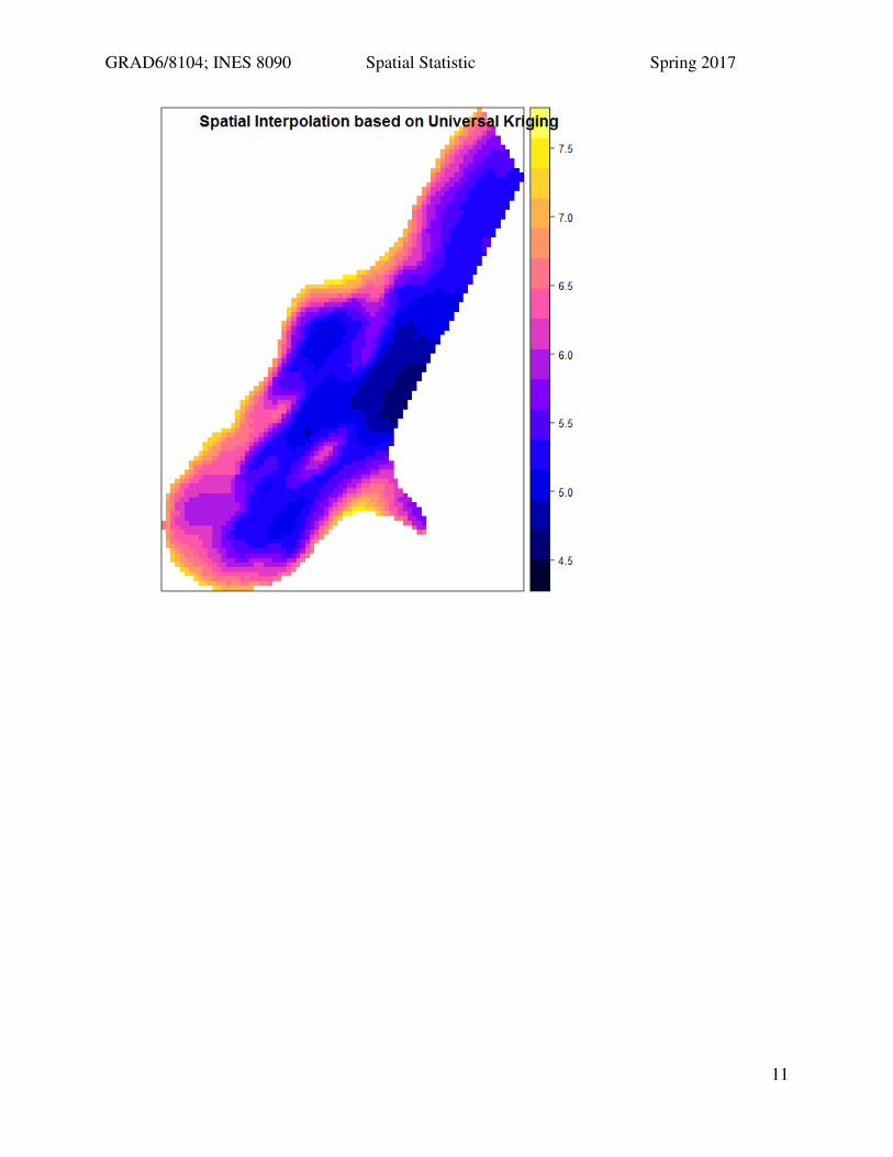
Since we know zinc concentration is a function of distance to the Meuse river, we could incorporate this into our Kriging-based spatial interpolation—i.e., using Universal Kriging Try the following command for Universal Kriging:

>zinc.uk=krige(log(zinc)~sqrt(dist),meuse,meuse.grid, model=zinc.fit) > spplot(zinc.uk["var1.pred"]) > title("Spatial Interpolation based on Universal Kriging")

GRAD6/8104; INES 8090 Spatial Statistic Spring 2017

11

GRAD6/8104; INES 8090 Spatial Statistic Spring 2017

12

Questions: Question 1: Conduct semivariogram analysis on the meuse dataset (using a different heavy metal variable instead of zinc) in the gstat package. Write (at least) a paragraph to interpret your semivariogram results. Question 2: Using the same variable that you picked in Question 1, conduct spatial interpolation using Ordinary Kriging and IDW algorithms. Write (at least) a paragraph to compare these two interpolation algorithms and interpret your spatial interpolation results. Question 3: Using the same variable that you picked in Question 1, conduct spatial interpolation using Ordinary Kriging and Universal Kriging. Write (at least) a paragraph to compare these two interpolation algorithms and interpret your spatial interpolation results. Question 4: Using the same variable that you picked in Question 1, test anisotropy in the meuse dataset. Note that you need to provide the R commands (code) that you use together with the results. Otherwise, you will receive ZERO credit.