Estimating global temperatures - statmos.washington.edu fileEstimating global temperatures! Peter...
31
Estimating global temperatures Peter Guttorp University of Washington and Norwegian Computing Center
Transcript of Estimating global temperatures - statmos.washington.edu fileEstimating global temperatures! Peter...

Estimating global temperatures!
Peter Guttorp!University of Washington!
and!Norwegian Computing Center!

Overview!
Data!Methods!Results!Joint work with Finn Lindgren, NTNU, Trondheim!
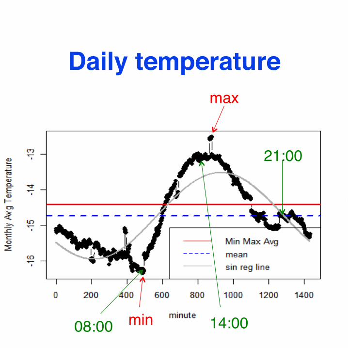
Daily temperature!max!
min!08:00! 14:00!
21:00!

Daily mean temperature!
Average of min and max!Which min and max?!Is it a good estimate of the actual mean?!Other approaches!


Homogenization!
miscalibrated!thermometer!
urbanization!
screen painted white?!summertime !correction!
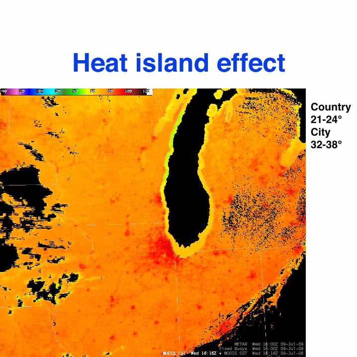
Heat island effect!Country!21-24°!City!32-38°!

Other inhomogeneities!
Visby airport, monthly means!
1960 1970 1980 1990 2000 2010
-1.0
0.0
1.0
Year
SMHI
- G
HCN

Global Historical Climatology Network!

GHCN network size!
1880 1900 1920 1940 1960 1980 2000
1000
2000
3000
4000
Year
Num
ber o
f obs
erva
tions Adjusted! Unadjusted!

Ocean temperatures!
ICOADS!2°x2° since 1800!

WM* V- Ti3 !b
! 4.n’
A k c WORLD METEOROLOGICAL ORGANIZATION ORGANISATION METEOROLOGIQUE MONDIALE
Secretariat of the World Meteorological Organization Geneva - Switzerland
Sec&tariat de 1’0rganisation MCthrologique Mondiale Genkve - Suisse
INTERNATIONAL LIST
SELECTED AND SUPPLEMENTARY SHIPS OF
LISTE INTERNATIONALE DE
NAVIRES S~LECTIONNES ET SUPPLEMENTAIRES
PRICEPRIX: Sw. fr./Fr. s. 5.-
I WMOjOMM - No 47. TP. 18 I 1955
12 B E L G I Q U E Navires s6lect ionn6s / Navires suppldmentaires
l e r j a n v i e r 1955
Nom du I nd i c a t i f Route ou Navire d appel des igna t ion de l a route
1 2 3
_I- Navires sQlec t ionn6s 1 ) A l b e r t v i l l e 2) Baudouinville 3) Char l e sv i l l e
- 4 ) Copacabana 5 ) E 1 i s abet hv i 1 1 e 6) LQopoldvi l le 7) Mar d e l P l a t a 8) We s t - H i nd e r
(Bateau phare)
ONAH ONBD ONCP ONCO O E L ONLD ONME
OTW
Navires suppl6mentaires 1) Belgian Pr ide ONBM
3) Escaut ONE0 2) Egypte ONEG
4) Espagne ONER 5 ) Louis Sheid ONLP
6) Mercator (Navire &cole) ORFA
7) Portugal ONPO
Anvers - Congo Belge Anvers - Congo Belge Anvers - Congo Belge Anvers - Congo Belge Anvers - Congo Belge Anvers - Congo Belge Anvers - Congo Belge
Mer du Nord
Anvers - Golfe du Mexique Anvers - Proche-Orient Anvers - Proche-Orient Anvers - Proche-Orient Anvers - Golfe du Mexique - Amhrique
du Sud
Divers voyages Anvers - Proche Or ien t
B E L G I Q U E Navires sdlect ionn4s / Navires surmldmentaires
13
Mdthode employde Type du Type de pour ob ten i r l a Type du Autres baromhtre lrhygrom&tre tempdrature de l ' e a u barographe Instruments
& l a sur face de l a mer
4 5 6 7 8
I Navires sdlect ionndz 1) 1 an. 1 psy. c r d c e l l e 2) 1 an. 1 psy. c r d c e l l e 3) 1 an. 1 psy. c r d c e l l e 4) 1 an. 1 psy. c r d c e l l e 5) 1 an. 1 psy. c r d c e l l e 6) 1 an. 1 psy. c r d c e l l e 7) 1 an. 1 psy. c r g c e l l e
8) 1 an, 1 psy. c r Q c e l l e
I_- Navires suppl6mentaireA 1) 1 an. 1 psy. c r Q c c l l e 2) 1 an. 1 psy, c r e c e l l e 3) 1 an. 1 psy. c r d c e l l e 4) 1 an. 1 psy. c r k e l l e 5) 1 an. 1 psy. ci-dcelle
6) 1 an. 1 psy. c r d c e l l e
7) .1 an. 1 psy. c rdce l l e
seau seau se au seau seau seau seau
se au
condenseur condenseur condenseur condense u r condc nseur
seau
co nde ns eur
1* 1* l* 1* 1- I** 1w
1"
* grande Qche l l e * p e t i t e dche l le

Ocean SST estimation!
Uses (essentially) EOFs !Separate LF and HF variation!Damped covariance beyond 5 Mm!No covariance beyond 8Mm!Reject data > 3.5 or 4.5 ese around the smoothed median value for each box and climatological period!(This can eliminate ENSO signal)!

ICOADS and GHCN!
1880 1900 1920 1940 1960 1980 2000
1000
2000
3000
4000
Year
Num
ber o
f obs
erva
tions
Global processes!Problems such as global warming require modeling of processes that take place on the globe (an oriented sphere). Optimal prediction of quantities such as global mean temperature need models for global covariances. !Note: spherical covariances can take values in [-1,1]–not just imbedded in R3.!Also, stationarity and isotropy are identical concepts on the sphere.!

Gaussian Markov random field model!! ! !Model parameters!! ! !Spatial climate!! ! !Weather anomalies!! ! !Temperature data!
!Data model: temperature ~ elevation + climate + anomaly!
θ
µ(u) θxt(u) θ,µ(u)yt,i θ,µ(ui),xt (ui)

Tesselation!Intro Models Fields End Spatial dependence Discretised models Projection
Piecewise linear representations
x(u) = cos(u1) + sin(u2) x(u) =P
k
k
(u) xk
Guiding principle
Attack the SPDE with local finite dimensional representationsinstead of covariances or kernels (subsets of Green’s functions)!
Finn Lindgren - [email protected]

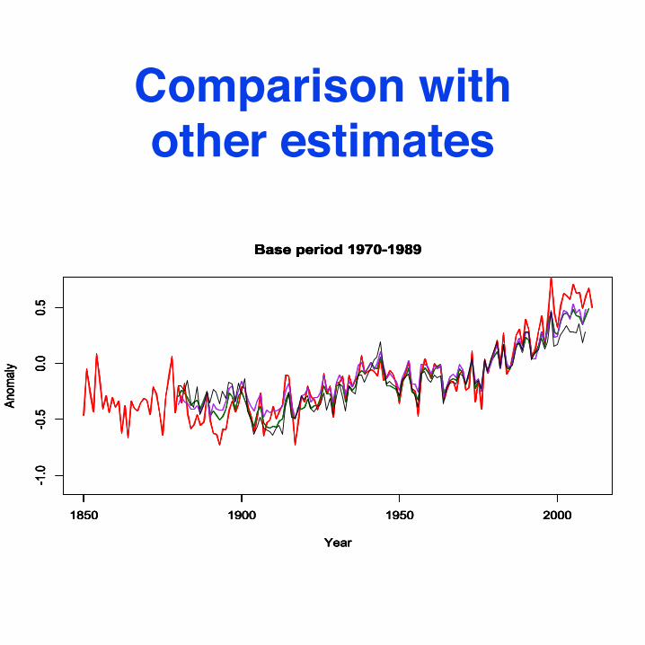
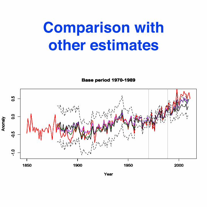
Other approaches!Hadley/CRU: Local kriging (within 5°x5° grid square). No between grid square correlation.!NOAA: K-L expansion using observed spatial covariance in reference period to estimate 5°x5° grid squares!GISS: Distance-weighted averaging in 8K equal area grid squares!BEST: Isotropic kriging on the square (much larger data set; only land data).!

Results!Elevation effect (-5.32,-5.26) °C/km!

Std dev of anomaly model (C)0 2 4 6 8
Correlation of anomaly model (C)0.0 0.2 0.4 0.6 0.8 1.0

Empirical Anomaly 1980 (C)−3 −2 −1 0 1 2 3

Trend estimate!
1880 1900 1920 1940 1960 1980 2000
-1.0
-0.5
0.0
0.5
Year
Anomaly

Comparison with other estimates!
1850 1900 1950 2000
-1.0
-0.5
0.0
0.5
Year
Anomaly
Base period 1970-1989

Comparison with other estimates!
1850 1900 1950 2000
-1.0
-0.5
0.0
0.5
Year
Anomaly
Base period 1970-1989
1850 1900 1950 2000
-1.0
-0.5
0.0
0.5
Year
Anomaly
Base period 1970-1989

Comparison with other estimates!
1850 1900 1950 2000
-1.0
-0.5
0.0
0.5
Year
Anomaly
Base period 1970-1989
1850 1900 1950 2000
-1.0
-0.5
0.0
0.5
Year
Anomaly
Base period 1970-1989
1850 1900 1950 2000
-1.0
-0.5
0.0
0.5
Year
Anomaly
Base period 1970-1989
Comparison with other estimates!
1850 1900 1950 2000
-1.0
-0.5
0.0
0.5
Year
Anomaly
Base period 1970-1989
1850 1900 1950 2000
-1.0
-0.5
0.0
0.5
Year
Anomaly
Base period 1970-1989
1850 1900 1950 2000
-1.0
-0.5
0.0
0.5
Year
Anomaly
Base period 1970-1989
1850 1900 1950 2000
-1.0
-0.5
0.0
0.5
Year
Anomaly
Base period 1970-1989
1850 1900 1950 2000
-1.0
-0.5
0.0
0.5
Year
Anomaly
Base period 1970-1989
1850 1900 1950 2000
-1.0
-0.5
0.0
0.5
Year
Anomaly
Base period 1970-1989

Adjusted vs unadjusted!
1880 1900 1920 1940 1960 1980 2000
-0.15
-0.10
-0.05
0.00
0.05
Year
Adju
sted
min
us u
nadj
uste
d
-0.6 -0.4 -0.2 0.0 0.2 0.4
-0.6
-0.4
-0.2
0.0
0.2
0.4
Adjusted
Unadjusted

2003 anomaly!Empirical Anomaly 2003 (C)
−6 −4 −2 0 2 4 6
Empirical Anomaly 2003 (C)−6 −4 −2 0 2 4 6
Adjusted!
Unadjusted!

North vs South!
1880 1900 1920 1940 1960 1980 2000
-1.5
-1.0
-0.5
0.00.5
1.01.5
Year
North
ern
minu
s Sou
ther
n an
omali
es
Adjusted data, integrated run