
A NONLINEAR MIXTURE AUTOREGRESSIVE MODEL FOR SPEAKER VERIFICATION
Introduction
The distribution of population is one of the fundamental inputs for many research tasks (such as urban planning facili-
ties allocation and quality of life assessment) because the dispersion of resources and energy among various geographical areas is strongly dependant on the population size (Hoque 2008) Traditional methods for the collection of population data involve a census which entails extensive planning surveying and data process-ing which is time consuming laborious and expensive (Lo 2006) Due to the huge financial investments involved census data such as those
Spatial Autoregressive Model for Population Estimation at the Census Block Level Using
LIDAR-derived Building Volume Information
Fang Qiu Harini Sridharan and Yongwan Chun
ABSTRACT The collection of population by census is laborious time consuming and expensive and often only available at limited temporal and spatial scales Remote sensing based population estimation has been employed as a viable alternative for providing population estimates based on indicators that make use of two-dimensional areal information of buildings or one-dimensional length information of roads The recent advancement of LIDAR remote sensing provides the opportunity to add the third dimension of height information into the modeling of population distribution This study explores the use of building volumes derived from LIDAR as a population indicator Our study shows the volume-based model consistently outperforms area and length-based models at the census block level Additionally the study examines the impact of spatial autocorrelation the presence of which violates the independence assumption of the traditional OLS models To address this problem a spatial autoregressive model is employed to account for the spatial autocorrelation in the regression residuals By incorporating the spatial pattern the volume-based spatial error model achieves a good-ness of fit (R2) of 85 percent with a significant improvement in model performance and estimation accuracies in comparison with its OLS counterpart The study confirms building volume as a more valuable indicator and estimator for block level population distribution especially if an appropriate spatial autoregressive model is adopted KEYWORDS Population estimation Lidar building volume spatial models
Cartography and Geographic Information Science Vol 37 No 3 2010 pp 239-257
provided by the US Census Bureau are usu-ally collected only at a fixed time period (eg once every ten years) and at a set of pre-defined geographic units (eg the census tract block group and block) The fact that census data are provided at a limited temporal and spatial scales restricts census datarsquos applications to only those that do not critically rely on the most current information of the population distribution at detailed levels
In addition to conducting a census every ten years the US Census Bureau also provides intercensal population count estimations at state county and city levels based on projection techniques (Smith 1998) but the estimates are not available at any finer geographical scale such as the tract or block level The US Census Bureau has recently introduced the American Community Survey (ACS) which aims at providing population information every year instead of every ten years The ACS selects a sample of households for surveying and provides yearly estimates based on this sample Currently only three-year estimates from 2006-2008 are available and five-year estimates are expected to
Fang Qiu University of Texas at Dallas 800 W Campbell Rd GR31 Richardson Texas 75080-3021 Tel 972-883-4134 E-mail ltffqiuutdallasedugt Harini Sridharan University of Texas at Dallas 800 W Campbell Rd GR31 Richardson Texas 75080-3021 E-mail lthxs065100utdallasedugt Yongwan Chun University of Texas at Dallas 800 W Campbell Rd GR31 Richardson Texas 75080-3021 Tel 972-883-4719 E-mail
ltywchunutdallasedugt
240 Cartography and Geographic Information Science
be available by the end of 2010 These estimates will be available only at the tract level or above but will remain unavailable to the more detailed (block group and the block) levels To support activities that need suitable population information at a fine-scale level for a given year between two consecutive decennial censuses (eg emergency response planning) population estimation is still needed At this scale reliance must be placed on third party often expensive complex commercial demographic models These models may provide reasonable estimation but often involve significant manpower for demographic analysis Due to the requirement to collect multiple inputs the suc-cess of the models relies heavily on the quality of these inputs and the performance of the models in earlier time periods which are not always reli-able (Qiu et al 2003)
In order to estimate population at various levels of detail remote sensing imagery and its derived datasets have been employed as viable alterna-tives in population prediction Remote sensing provides a synoptic view of a large area which can be acquired at a small and regular time interval or within a short period of time when it is needed (Lo 2006) With the right techniques remote sens-ing based population estimation can serve as a cheaper and less laborious replacement for com-mercial demographic models Over the past 40 years a variety of remote sensing products with different spatial resolutions have been employed to estimate population at different scale levels For example low to medium resolution satellite images such as Landsat TM imagery have been used to conduct city level population estimation (Lisaka and Hegedus 1982 Qiu et al 2003 Wu and Murray 2007) while large-scale aerial photo-graphs have been employed to support the mod-eling of population counts at a community level such as the census tract (Porter 1956 Dueker and Horton 1971 Lo 1989) The advent of IKONOS Quickbird and other very high spatial resolution satellite imagery enables us to drill down to even more detailed levels such as the block and block group (Haverkamp 2004 Lu et al 2006 Liu et al 2006 Chen 2002) The increasing refinement in spatial resolutions for aerial and satellite images and their growing availability to the public have motivated a wider adoption of remote sensing technology for population estimation aimed at achieving better accuracy at a finer scale level than was previously possible
The promise of remote sensing technology for population estimation lies in the fact that its derived data products contain rich information on the
distribution of human settlements which can serve as reliable indicators of population In many past studies a variety of indicator variables of human settlement distribution have been extracted from remotely sensed imagery to provide timely and detailed population estimation including extent of urban development (Tobler 1969 Ogrosky 1975 Lo and Welch 1977 Lisaka and Hegedus 1982 Weber 1994) area of residential land use (Lo 1989 Wu et al 2005 Lu et al 2006 Qiu et al 2003) counts of dwelling buildings (Lo 1995 Wu et al 2008 Lwin and Murayama 2009) length of roads (Qiu et al 2003) and spectral index of pixel values (Liu et al 2006 Harvey 2002) Utilization of these variables to model population distribution makes use of only two-dimensional (2-D) areal or one-dimensional (1-D) length information The recent development in Light Detection And Ranging (LIDAR) technology provides the opportunity to go beyond this limit (Xie 2006) With the accurate height information acquired by LIDAR we now can incorporate a third dimension of information in population estimation In this research we will explore the utilization of the volume of residen-tial buildings as a potential indicator to estimate population distribution at fine scales such as the census block
Resolution refinement in remote sensing data offers the opportunity to model population at finer scales but it also demands a corresponding enhancement in population estimation methodol-ogy Previous approaches to population estimation have been largely based on ordinary least square (OLS) regression The OLS approach assumes that observations are independent of each other ignoring the possible spatial relationship that may exist between them This assumption may not be valid with variables representing a geographically varying phenomenon such as population because when the spatial scale moves down especially to the block level the spatial autocorrelation of population among neighboring blocks is likely to become stronger (Brown 1995) This may lead to the violation of the OLS independence assump-tion a problem that needs to be addressed using an improved methodology to ensure a valid model of population estimation
The purpose of this research is to test if the volume of residential buildings facilitated by the latest LIDAR remote sensing techniques can serve as an effective indicator variable to estimate popu-lation at the block level The effectiveness of this 3-D volume based population estimation will be assessed using comparisons with traditional 2-D and 1-D approaches based on the area of residential
Vol 37 No 3 241
buildings the area of residential land use and the length of road networks This paper proposes the use of spatial autoregressive regression to address the spatial autocorrelation problem of traditional OLS models when applied in fine-scale population estimation This study will examine the possible presence of spatial autocorrelation in block level population and develop appropriate spatial models according to its type The accuracy and robustness of these spatial models will be compared with those of the OLS models
Literature ReviewEstimation of population using remote sens-ing products dates back to the 1960s when Nordbeck (1965) found an exponential relation-ship between the population and area of urban settlement based on allometric growth models This relationship was tested by Tobler (1969) who correlated the radius of built-up areas with population and established a correlation coeffi-cient of 087 Popularization of Landsat imagery in the 1970s in land use land cover mapping promoted the use of this data for population estimation at city and census tract levels Lo and Welch (1977) estimated the population of Chinese cities by extending Nordbeckrsquos model to the measurement of built-up area extracted from Landsat images and achieved a correlation coefficient of 082 Chen (2002) used Landsat TM data to classify residential land uses into dif-ferent density levels and modeled census counts as a function of the area of three residential land uses at high medium and low density levels Qiu et al (2003) modeled the growth in popula-tion at city and census tract levels using Landsat TM based change detection It was also found that new developments in the road network were a better indicator of population growth than the change in urban land use These studies usually estimate population at a predetermined geo-graphic unit such as the city county or census tract with population counts regressed against the area of urban or residential land use or length of road networks aggregated to that geo-graphic unit Characteristics derived from the individual pixels in satellite images have also been utilized as population indicators Lisaka and Hegedus (1982) established a mathemati-cal relationship between population density and the radiance measured from Landsat data to estimate the counts Li and Weng (2005) correlated population with various pixel level
variables using spectral signatures principal components vegetation indices textures and temperatures extracted from Landsat TM data Harvey (2002) classified each pixel of Landsat TM data to delineate residential area and used an EM algorithm to iteratively regress the popu-lation at each pixel level with its spectral values and adjust the results through redistributing the errors at the aggregation zone into each of the individual pixels
With the availability of high spatial resolution remotely sensed imagery residential areas can be delineated with a greater precision and accu-racy so that the estimation of population can be attempted at finer levels To estimate population at the block group level Almeida et al (2007) performed a multi-resolution segmentation on a Quickbird image to delineate homogeneous resi-dential areas of different occupation density based on spectral geometrical and topological features of the segmentations as well as their context and semantics With improvements in image resolution and processing technologies it is now possible to model population based on the number of indi-vidual dwelling units automatically determined by object-oriented or object-based classifications (Haverkamp 2004 Zhang and Maxwell 2006) rather than the laborious manual counting from aerial photographs previously employed in many earlier studies (Green 1956 Hadfield 1963 Binsell 1967) However as early as Green (1956) it was noticed that population was often underestimated when using dwelling counts derived from aerial photo-graphs because the number of vertically stacked dwelling units cannot be easily identified from the 2-D photographs This problem persists in the automatic determination of dwelling units from very high resolution satellite images because usually only the roof of the buildings is visible from the satellitersquos perspective
Population estimation should be improved by incorporating the third dimension height infor-mation which can provide an insight into the structure of the dwelling units The potential of LIDAR data for the extraction of building height (Maas and Vosselman 1999 Barnsley et al 2003) and the reconstruction of the 3-D building structure (Hongjian and Shiqiang 2006 Gurram et al 2007 Sampath and Shan 2007) has been explored in the recent literature However population estimation using LIDAR-derived building structure informa-tion is still in its nascent stage and a search in literature yielded only a few related works Xie (2006) proposed a theoretical framework of areal interpolation for population to the level of housing
242 Cartography and Geographic Information Science
units The housing units were extracted and classi-fied based on high resolution DOQQ imagery and LIDAR data The population was then allocated to each unit based on a variety of factors one of which was the volume of buildings This theoreti-cal framework could be used to estimate popula-tion at any aggregation zone level including the census block However no actual population esti-mation was conducted by the authors with detailed accuracy assessment Wu et al (2008) developed a deterministic equation for estimating popula-tion at block and sub-block levels by multiplying the number of housing units with the occupancy rate and average number of people per unit The number of housing units was derived based on the ratio between LIDAR-derived building volume and the average space per unit The research was able to achieve an average percent error of 011 at block level because in addition to the remotely sensed building volume detailed information on the occupancy rate average space per housing unit and average number of persons per household was also included These variables however are not always available for intercensal years
The research reported here is based on the premise that the volumetric information of a building can serve as a better indicator than building counts or 2-D area data for population estimation at a fine-scale level Volumetric information derived from building heights automatically extracted from LIDAR can provide a better surrogate for the number of residential units in buildings with one or more stories (ievertically stacked structure) However an appropriate methodology must be employed to take advantage of this detailed information Most remote sensing based population estima-tion models utilize ordinary least squares (OLS) to fit a multivariate regression between popula-tion counts and various demographic indicators (Wu et al 2005) Ordinary least square models assume the independence of the observations (Bailey and Gatrell 1995) which is rarely true for a geographically varying variable such as popula-tion The assumption of OLS ignores the spatial process of the underlying phenomena and their effect on the estimation Modeling of geographi-cally varying variables based on OLS is therefore likely to produce biased or inefficient estimation (Anselin 1988)
For example Lo (2008) discovered that the relationship between population and classified land coverland use is not constant across space (non-stationarity) a problem that OLS models cannot deal with He applied a local geographically weighted regression (GWR) model for popula-
tion estimation that permits the regression coef-ficients thus derived to vary geographically and achieved improved estimation accuracy over the OLS model of 28 percent at the census tract level Lo (2008) suggested that the spatial non-stationarity problem can be mitigated if smaller spatial units are used At finer scales such as the census block level the spatial process determining population does not vary as rapidly as do processes at much coarser levels and can often be considered to be stationary
However another problem appears at this level which is the presence of spatial autocorrelation In the case of population it means their counts tend to have similar values within a short distance As a result spatial autocorrelation tends to be more pronounced at a finer-scale level because population counts vary minimally from those of neighboring units when aggregated in smaller zones such as census blocks According to the Geographic Area Reference Manual provided by the US Census Bureau (1994) census blocks in urban and surrounding suburban areas are designed as relatively small grids with road networks and may be disrupted here and there by water features topographic relief and transportation features such as rail yards and airports If a block contains an array of residential buildings then it is highly probable that its neighboring blocks also contain similar residential developments leading to a cor-responding correlation in the population count with neighboring blocks
To address this spatial autocorrelation issue spatial autoregressive models (Anselin 1988) need to be used in place of OLS models The current study implements this by first examin-ing the spatial pattern in the dependent variable and the OLS regression residuals using a set of spatial diagnostics Then an appropriate spatial autoregressive model is selected which explicitly accounts for the spatial autocorrelation present in the population estimation
Study Area and DataTo test our proposed approach we selected a part of Round Rock Texas as our study area (Figure 1) Located 15 miles north of Austin Round Rock is a suburban city in the Austin-Round Rock metropolitan area and the home of a major computer manufacturer Dell Inc According to American FactFinder by the US Census Bureau it is one of the fastest growing cities in the US with a population of 63136 in 2000 and an esti-
Vol 37 No 3 243
mate of 86175 in 2006 a 4095 percent increase over a period of six years A subset of the city located between 30deg30prime N and 30deg31prime N and
between 97deg39prime W and 97deg41prime W was used in this study which covered an area of 10 square km comprised 220 buildings and had a total popu-
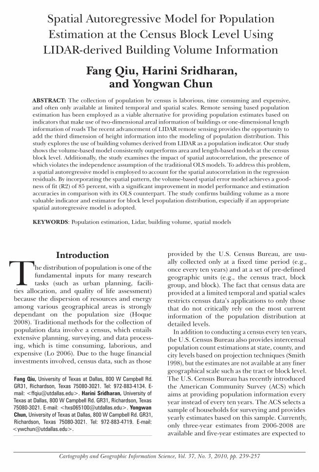
Figure 1 Census block population density of the study area
244 Cartography and Geographic Information Science
lation of 9550 residents in 2000 This is a typi-cal residential area with a mixed composition of single and multifamily buildings
The population data were obtained from the 2000 US Census Bureau block data (Figure 1) The 220 blocks in the study area had populations ranging from 0 to about 1290 people per block in 2000 Since a non-zero intercept model is to be developed blocks with zero population were eliminated which resulted in 175 blocks available for subsequent analyses The blocks are mostly near rectangular or square grids with a few large irregularly shaped blocks in the central part of the region due to a water body A visual examination of the population map suggested a noticeable positive spatial autocorrelation in the distribu-tion of population For example blocks with high population density were clustered predominantly in the north-western and lower southern portion of the study area
The various population indicators used in the study including the area of residential land use the length of road networks and the area and volume of residential buildings were either extracted from remote sensing imagery or obtained from remote sensing derived GIS data provided by City of Round Rockrsquos GIS Information Center The parcel-level land use and road network GIS data were both derived from 2006 aerial photographs using a combination of automated digital image processing and visual photo interpretation The parcel level land use data includes 16 categories and only the categories for residential land use (that is single- two- and multi-family) were retained for analysis The road networks in the study area are mostly city streets surrounding the blocks except for a US Highway running through the middle of the city Since a block is often surrounded by roads or other linear features and there may possibly be a few internal roads within the block one of which may go completely through the total length of the street network surrounding each block and the internal roads are used as an indicator of popula-tion per block
Building footprints were derived from high-reso-lution aerial photographs by Round Rock GIS Information Center through combined digital image classification and visual photo interpretation aerial photographs are the most accurate source currently available for footprint data Building footprints can also be extracted automatically using LIDAR data (Maas and Vosselman 1999 Barnsley et al 2003) However since the average resolution for most LIDAR data currently available for cities is often coarser than that of high-resolution aerial
photographs and a perfect differentiation between buildings and nearby tall trees is still very chal-lenging the accuracy of the subsequent building volume calculation will be compromised unless substantial post-processing manual editing is con-ducted Buildings used for residential purposes were identified by overlaying them with the parcel level land use data described above Both land use and building footprint data were available only for the year of 2006 but block-level population census data were available for the year 2000 Visual comparison of 2000 and 2006 aerial photographs indicated that no buildings present in 2000 were demolished in 2006 and the only changes since 2000 were new housing developments In order to derive a footprint map for the year of 2000 any new housing developments that appeared only on the 2006 aerial photographs were eliminated The LIDAR dataset was collected by Williamson County in 2006 with an average point spacing of 14 m and a vertical accuracy of 10 cm A similar approach was used to eliminate all LIDAR points corresponding to the buildings constructed after 2000 to match the 2000 census data
The heights of residential buildings were deter-mined using a method aimed at extracting height information from LIDAR point cloud data First a two-way buffer along the boundary of the build-ing footprint is created with a buffer distance of one foot on both sides of the boundary (Figure 2) This buffer serves as an exclusion zone that excludes the LIDAR points potentially bounced off from the walls of the buildings Then a one-way buffer is performed along the outer boundaries of these exclusion zones using a buffer distance of two feet The LIDAR points within the outer buffer zone are primarily those corresponding to returns from the ground The median elevation of the points within this buffer zone is then cal-culated and taken as the elevation of the ground around the building The use of median value instead of the mean prevents the influence of the extreme values from points reflected from tall trees or low pits Another one-way buffer is then followed along the inner boundaries of the exclusion zones also with a buffer distance of two feet The median elevation of the points within the inward buffer zone is used as the elevation of the building roof The use of the median value in this case prevents extreme values from the points reflected from TV antennas chimneys and other above-roof structures to influence the analysis Next the difference between the median elevations of the inward and outward buffer zones is computed and assigned to each building as the above-ground
Vol 37 No 3 245
height of the building The building height thus determined is then multiplied by the area of the building footprint to obtain the volume of indi-vidual buildings Finally the volumes of all the individual buildings within a block are aggregated for use as a block level indicator variable in the subsequent regression analysis
MethodologyThe volumes of residential buildings derived based on the additional height information fur-nished by the LIDAR data can serve as a valid and reliable indicator for population estima-tion an OLS based allometric growth model is first developed The results from this model are compared with similar OLS models using the traditional indicator variables such as area of residential buildings area of residential land use and length of road network in a block To
determine the potential presence of spatial autocorrelation in the model and to identify an appropriate spatial autoregressive model to address it a series of diagnostics were per-formed
To estimate model parameters and to evaluate model performance we divided the study area into north and south sections along the US Highway 79 that passes through the region (Figure 1) The south section of the study area contains 102 blocks and was used for training the models and the north section has 73 blocks used for testing the models Unlike the commonly used spatially random selection of training and testing sites the practice of dividing the study area into two sections preserves the spatial contiguity of the census blocks and allows the construction of the spatial connectivity matrix a requirement of the spatial autoregressive model for both train-ing and testing purposes A set of various error measures are employed and calculated using the
Figure 2 Building height determination from LIDAR
246 Cartography and Geographic Information Science
north section testing data in order to evaluate the performance of models derived from the training data in the south section
The OLS ModelsThe OLS models used in this study are based on the widely used allometric growth equation (Nordbeck 1965) which suggest an exponential relationship between population (P) and built-up area (A) as shown in Equation (1)
(1)
where α and b are model coefficients The allometric growth equation has been modified by using other 1-D or 2-D population indicator variables For example Tobler (1969) replaced the built-up area in the original allo-metric growth equation with the radius of urban development (r) to estimate population assum-ing that cities are usually circular in shape We extended this idea by substituting built-up area with the volume of residential buildings aggre-gated at the census block level as shown in fol-lowing equation
(2)
where β is the rate at which the population (P) changes with the volumes of residential build-ings (V) When the value of β is less than 1 it indi-cates a negative allometry where the population grows at a slower rate than the volumes of the residential buildings A β value close to one indicates that the growth rates of both variables are equal and population growth is in a state of isometry A positive allometric growthmdashwhere the population grows at a higher rate than build-ing volumemdashoccurs when β is greater than 1
In order to fit a regressive model of population to a volume of residential buildings using OLS logarithmic transformation is performed to the both sides of the allometric growth equation (2) As a result the original exponential equation is converted into a linear form as follows
(3)
A scatterplot of the log of building volumes versus the log of population at the block level confirms there is a strong linear relation-ship between the two variables (Figure 3) The Pearsonrsquos correlation coefficient between popu-lation and building volume was 0914 The log-arithmic transformation is often performed to make counts data (which is commonly assumed
to follow a Poisson distribution) normally dis-tributed It also ensures a linear functional form for the allometric growth Equation ()
The OLS model of population estimation involves fitting a linear statistical relationship (Burt and Barber 1996) between a dependant variable (Y) and one or more independent variables (X)
(4)
where β are regression parameters and e is the residual The best linear unbiased estimates of the regression parameters are determined by minimizing the sum of squares of the residuals (e) In this study population at the census block level is first estimated using the volume of resi-dential buildings based on the linearized allo-metric Equation (3)
For comparison OLS models of population estimation were also developed based on vari-ous traditional 2-D and 1-D indicator variables including area of residential buildings area of residential land use and length of road network The total area of residential buildings in each census block was estimated using the residential building footprint data The total area of residen-tial land use was aggregated from the parcel level residential land use data The area of residential land use is different from (and larger than) that of the residential buildings because it also includes the area of the parcel land surrounding the build-ings The length of the roads around a block was summed and used as another indicator variable for population estimation To be consistent with the volume-based model (Equation (3) logarithmic transformation of these 2-D and 1-D variables and the population counts were performed
Spatial DiagnosticsSpatial autocorrelation is a direct implication of Toblerrsquos law (Tobler 1970) which states that things nearer to each other are more similar than those farther away Spatial autocorrelation happens commonly with geographically varying attributes such as population as suggested by the visual examination of the block-level pop-ulation distribution in Figure 1 where blocks with similar population counts appear to clus-ter in space The existence of spatial autocor-relation makes the use of OLS-based regression questionable because its assumptions require that the observations are independent of each other or the residuals from the OLS estimation are uncorrelated (Haining 1990) Violation of these assumptions may result in biased and inef-
bAα= timesP
βα Vtimes=P
)()( VLogLog sdot+= βαLog(P)
eX += βY
Vol 37 No 3 247
ficient estimation of the parameters of the linear regression
In addition to the above casual visual examination of Figure 1 which suggests a spatially autocorre-lated data distribution a series of diagnostics can also be performed to statistically determine the presence of spatial autocorrelation and to iden-tify the form of the spatial process (spatial lag or spatial error) causing it Moranrsquos I (Moran 1950) is often used to measure the degree of spatial autocorrelation of the dependant variable and the residuals of the OLS model Albeit useful in identifying the general misspecification of the OLS model Moranrsquos I falls short of providing any insight into the form of the spatial process causing the autocorrelation Therefore further evaluation is needed to decide which of the two common spatial processes spatial lag or spatial error is the cause
Lagrange Multiplier (LM) tests can be used for this purpose (Anselin 1996) There are two differ-ent types of LM tests LM Lag and LM Error The LM Lag test evaluates if the lagged dependent variable should be included in the model and the LM Error test assesses if the lagged residual should be included Additionally Robust LM tests can be conducted to verify if the spatial lag dependence is robust and therefore spatial error dependence can be ignored or vice versa
Spatial Autoregressive ModelsThe biased and inefficient results of the OLS models that are due to the presence of spatial autocorrelation necessitates the adoption of new regression approaches that can explicitly account for the autocorrelation Without taking spatial autocorrelation into consideration the
Figure 3 Relationship between population and volume of residential buildings
248 Cartography and Geographic Information Science
OLS models may result in biased and inconsis-tent model coefficients with inefficient variance estimates and incorrect confidence intervals which may cause the commitment of Type 1 errors by rejecting the null hypothesis when it is actually true (Anselin 1988 Bailey and Gatrell 1995) In simple terms spatial autocorrelation may cause the researcher to conclude that a rela-tionship exists when that is not actually the case Two common spatial autoregressive models can be employed the spatial lag model and the spa-tial error model
In the spatial lag model the value of a dependant variable Y at a location is modeled as a function of the independent variables X in that location as well as the values of the dependant variable at the neighboring locations that is the spatial lag A spatial lag is basically the weighted average of the dependant variable values at the neighboring locations (Anselin 1988) included as an additional explanatory variable in the model as shown in the following equations
Y = pWY + Xβ + ε (5)
or
(6)
where ρ is the coefficient of the spatial lag com-ponent ε is white noise W is a spatial weight matrix and I is an identity matrix
The spatial error model addresses the spatial autocorrelation existing in the regression residuals ( ε ) of the OLS models The value of the dependent variable Y in a location is redefined as a function of the independent variables X and the regression residuals of the neighboring location that is the spatial error A spatial error is fundamentally a weighted average of the individual residuals of the neighboring locations which is added into the model as an additional explanatory variable shown in the following equations
(7)
or (8)
where ρ is the coefficients for the spatial auto-correlation
In this paper a spatial weight matrix W is defined as a row standardization of the first order spatial contiguity matrix C whose element cij has 1 if census blocks i and j share a common boundary or vertex or 0 otherwise While only the first order
neighbors are considered in W spatial influence is not limited to just immediately adjacent neighbors The matrix (I minus ρ W)minus1 being used in the spatial lag models (Equation (6)) and spatial error models (Equation (8)) incorporates the influence of higher order neighbors (LeSage and Pace 2009) Unlike the W which is a sparse matrix with 0s for all the higher order neighbors this matrix is no longer sparse as a consequence of the inverse operation Since most of the elements in this matrix have a non-zero value the influence of higher order neighbors is implicitly considered in the spatial autoregressive models As mentioned earlier such a spatial weights matrix requires that testing and training data be based upon the division of the study area into two regions so that the spatial contiguity of the samples will not be disrupted by a commonly used spatially random selection scheme Similar spatial autoregressive models were also developed using the other 1-D and 2-D indicator variables so that the results of these models could be directly compared
Measures of Estimation ErrorTo assess the accuracy of the population estima-tion models derived from the 102 census blocks in the training data several error measures were computed based on the difference between the true population (P) and estimated population (Prsquo) of the 73 census blocks in the testing dataset These measures included root mean square error adjusted root mean square error mean absolute percentage error median percentage error and population weighted percentage error Detailed equations for these measures are shown in Table 1 Root mean square error (RMSE) computes the square root of the mean squared error for the census blocks and is widely used to assess popu-lation estimation models (Fisher and Langford 1995) If the population of the blocks varies greatly the blocks with high populations tend to have large estimation errors and therefore will heavily affect the RMSE measure while blocks with low populations tends to have small esti-mation errors and less influence to the RMSE measure For this reason the adjusted root mean square error (Adj-RMSE) was proposed (Gregory 2000) which computes the square root of the mean squared percentage error so that the drastic impacts of the blocks with extremely large populations can be avoided To avoid the possibility of accuracy overestimation due to cancelling out of negative and positive errors the Mean Absolute Percentage Error (MAPE)
ερβρ 11 minusminus minus+minus= )()( WIXWIY
εξρξξβ +=+= WX Y
ερβ 1minusminus+= )( WIXY
Vol 37 No 3 249
can be computed which takes the average of the absolute percentage error
The inclusion of percentage errors in Adj-RMSE and MAPE however may make them dispropor-tionally affected by the blocks with extremely small population because the same amount of estimation error in population counts may lead to a larger percentage error when the true population of the block is small To overcome the problem caused by the impacts from both extremely large and smaller values Qiu et al (2003) used the Median Absolute Percentage Error (MedAPE) which is the 50th percentile of the local absolute percent-age error Qiu et al (2003) introduced another error measure called Population Weighted Mean Absolute Error (PWMAE) which uses estimated population as a weight to normalize the absolute percentage error This measure has the advantage of eliminating the effects of extreme populations
MedAPE and PWMAE are believed to be more objective error measures that are not heavily impacted by blocks with either extremely high or low populations
Results and DiscussionThe results of the 3-D volume based model using the traditional OLS approach were compared with those derived from the OLS models based on conventional 2-D and 1-D popu-lation indicators such as area of resi-dential buildings area of residential land use and length of road net-work Table 2 gives the coefficient of determination (R2 and pseudo R2) Akaike Information Criterion (AIC) computed from the train-ing data and the five measures of estimation error computed for the testing data Only the results of the spatial error models are included in line with the spatial diagnostics discussed below
The R2 for the OLS models the pseudo R2 for the spatial models and AIC all reveal the goodness of fit of a specific model to the training data Specifically R2 and pseudo R2 reflect how much variation of the population in the training area is explained by its respective indicator variable ie whether or not the variable is a strong population indicator The Akaike
Information Criterion is a model selection crite-rion based on the distance between the estimates of the model and the true values which allows models of different types to be compared directly (Akaike 1974) A smaller AIC value indicates a better goodness of fit and therefore the model with the least AIC is regarded as the best model Since the OLS models report goodness of fit using R2 while the spatial autoregressive models use pseudo R2 they are not directly comparable (Veall and Zimmermann 1996) Therefore AIC is the best measurement to compare OLS and spatial autoregressive models
Among the four OLS models the residential building volume based model achieves the highest R2 of 08361 indicating a strong fit for the training data The volume- based OLS model also demon-strates consistently better population estimation
Measures Formula
Root Mean Square Error (RMSE)
Adjusted Root Mean Square Error (Adj-RMSE)
Mean Absolute Percentage Error (MAPE)
Median Absolute Percentage Error (MedAPE)
Population Weighted Mean Absolute Error (PWMAE)
t
t
tt
N
)P(PRMSE
N
1t
2sum minus= =
t
t
NAdj_RMSE
N
1t
2
tP
)t
Pt
(Psum
==
minus
tPtPtP
Median100MedAPEminus
times=
tN
tN
1t tPtPtP
100MAPE
sum=
minus
times=
sum=
sum=
minustimes
times=tN
1itP
tN
1t tPtPtP
tP
100PWMAE
Table 1 Error measures based on the difference between the estimated and the true population
250 Cartography and Geographic Information Science
when applied to the testing area evidenced by the apparently lower values for all five error measures when compared with those of the 2-D area and 1-D road length based OLS models
It is also observed that the indicator variables based on the characteristics of individual buildings (building volume and area) have better goodness of fit measures than parcel- level land use area and road length Since residential buildings can provide more precise information on the actual distribution of the population while parcel- level land use and road network are only proxies of where the population may be located it is under-standable that the two building- level indicator variables can better explain the variations of the population in the training data For the same reason one would expect that these indicators would also produce better population estimation when the OLS models are applied to the testing area However this is only true for the building- volume based model but not for the building area based model As a matter of fact out of the five measures of estimation error the building area based model only has two measures (RMSE MedAPE) smaller than those of the land use area based model and four measures (RMSE Adj-RMSE MedAPE and PWMAE) smaller than those of the road length based model
A high goodness of fit (R2 = 08153) obtained using training data accompanied by inconsistent error measures derived from the testing data are often an indication of possible over-fitting of the
model to the training data Even with higher-reso-lution images building area is not a stable indi-cator variable for population estimation This is probably because ldquobuilding areardquo covers only the area of the building footprint rather than the total area of all the residential units within the building Consequently the population living in buildings with vertically stacked residential units is likely to be underestimated and the population in one-story buildings overestimated In contrast the building volume measure which embeds addi-tional third dimension information on height is the actual total volume of all the residential units in the building Consequently the ability of the LIDAR data to inform about the vertical stacking of the buildings makes volume a stable indicator of population at the residential unit level which is the finest level of detail at which quantitative estimation of population can be currently achieved using remote sensing data This explains why the building volume model has been demonstrated to be both a stronger population indicator and a more accurate estimator than the building area
Another interesting finding is that at the block level the road length based model when com-pared with that of the land use area based model has lower accuracies in population estimation for the testing area as revealed by the larger errors for four of the five measures (RMSE Adj-RMSE MAPE and PWMAE) This disagrees with what was previously found at much coarser scales (Qiu et al 2003) where at both the city and census tract
ModelsR2
Pseudo-R2
AIC RMSE Adj RMSE MAPE MedAPE PWMAEMoranrsquos I
of residuals(p value)
OLS
Building volume based 08361 13104 2842 04023 2834 1869 271001708
(00073)
Building area based 08153 13941 5358 07268 5608 3799 571801305
(00257)
Land use area based 05087 20788 5362 04381 3972 4349 383204020
(00000)
Road length based 06433 18548 24450 09090 4885 3871 2151302235
(00011)
Spatial Error Models
Building volume based 08498 12884 2817 02880 2374 1816 242700203
(03317)
Building area based 08244 13896 3507 04840 3386 2059 349200160
(03525)
Land use area based 06666 18961 5388 04400 3998 4382 3855-004463(06456)
Road length based 07068 17855 7477 05460 5024 5740 6278-00337
(05945)
Table 2 Comparison of different population estimation models
Vol 37 No 3 251
levels population growth models based on road development were mostly better than those based on land use change detected in satellite imagery The fact that road networks traverse cities and census tracts but not always census blocks may help to explain the contradicting results obtained at these two different scales The use of high spa-tial resolution aerial photographs to derive parcel level land use as opposed to utilizing low spatial resolution TM satellite imagery to obtain urban land use may also contribute to the difference in findings This clearly demonstrates the famous
ldquomodifiable area unit problemrdquo in which the dif-ferent results may be expected from data with different geographic units (here census blocks versus tracts or cities) or scales
In order to use the OLS models for real world population estimation the models need to be vali-dated for the OLS assumptions of normality and independence To test for the normality of the log
transformed population counts graphic diagnostics and a statistic significant test were conducted For the graphic diagnostics a normal QQ-plot of the regression residuals from the volume-based OLS model was produced (Figure 4) When the quantile of the regression residual is plotted against the quantile of the standard normal probability distri-bution it is observed that the points approximately lie on a straight line verifying that the residuals are normally distributed
To assess the statistical significance the Jarque-Bera test that measures the departure from normal-ity based on skewness and kurtosis was performed (Jarque and Bera 1980) The null hypothesis of the Jarque-Bera test is that the skewness and kurtosis are jointly zero in other words the data tested comes from a normal distribution This test resulted in a Jarque-Bera statistic of 18909 with a p value of 03885 failing to reject the null hypothesis at the 95 percent confidence level and
Figure 4 Normal QQ-Plot of the regression residuals of the OLS volume based model
252 Cartography and Geographic Information Science
therefore reconfirming that the distribution of the OLS residuals is normal
A set of spatial diagnostics described above were also used to test the independence assumption of the OLS models based on both the dependant variable (ie log of population) and the regression residuals Moranrsquos I for the dependent variable illustrated a significantly positive spatial autocor-relation in population (with a Moranrsquos I value of 05587 and p value of 00000) This concurs with the conclusions drawn from the visual examination of the block level population map (Figure 1) The volume indicator variable of the OLS model can partially account for the spatial autocorrelation in population However the residuals of the OLS model still present a significant level of positive spatial autocorrelation having a Moranrsquos I value of 01708 and p value of 00073 The presence of spatial autocorrelation in the data violates the independence assumption of the OLS regression and demands explicit treatment with a spatial autoregressive model
In order to select between the spatial lag and spatial error models LM and LM Robust tests were performed The LM Lag test and LM Lag Robust test both resulted in positive test statistics (04063 and 01890 respectively) but with p values of 05239 and 06637 respectively they fell short of rejecting the null hypothesis of zero lag depen-dence at the 95 percent confidence level The LM Error and LM Error Robust tests do however reject the null hypothesis of zero error dependence with significant p values of 00434 and 00494 respectively The LM and LM Robust tests thus consistently indicate that the spatial error model is the preferred alternative to use for addressing the spatial autocorrelation in the data
Similar tests for the normality and independence assumptions were performed on the other OLS models (detailed results not shown) The normal-ity tests confirmed that the regression residuals of the OLS models are all normally distributed In addition the spatial diagnostics detected the misspecification of these OLS models due to the presence of spatial autocorrelation and determined the spatial error model as the appropriate model for population estimation The Moranrsquos I values in Table 2 show that while the residuals of the OLS models have a significant positive spatial autocor-relation spatial error models show no signs of spatial autocorrelation of the model residuals as evidenced by their low absolute Moranrsquos I values and large p values (gt005)
The spatial error models were built using the four indicator variables with the training data
they were subsequently applied to the testing data for population estimation A general trend similar to that for the OLS models was observed for the spatial autoregressive models with the building volume based model providing the best results followed by the building area based model The building volume based model again achieved the highest goodness of fit (pseudo R2 = 0 8498) and consistently produced the lowest values for all the five error measures reconfirming volume as both the strongest indicator and the most accurate estimator for population Models based on the characteristics of individual buildings (volume and area) outperformed models based on the charac-teristics of larger geographic units not only in the modelsrsquo goodness of fit but also in their estima-tion accuracy In contrast to the OLS models the building area based spatial model now has all five error measures lower than the road length based model and four error measures lower than the land use area based model with the only excep-tion being a slightly larger value in the adjusted RMSE an error measure heavily affected by extreme values This consistent improvement is attributable to the ability of the spatial error model to account for the autocorrelation in the residuals caused by unknown factors not included in the model One of these unknown factors is obviously the aforementioned third dimensional building height information The spatial error model based only on building area was able to partially compensate for the missing height information and achieve estimation accuracy closer to that of the OLS model based on building volume which included the missing factor of height
The addition of the height information in the volume based spatial error model further enhanced the modelrsquos ability in population estimation evi-denced by the reduction in values of error measure-ments For example the more objective PWMAE measure is now reduced by almost 10 percent (from 3492 percent to 2427 percent) when the additional height information is included Compared to its OLS counterpart the building volume based spatial model also exhibits improvement in estimation accuracy with a noticeable reduction in the error measures The likelihood ratio (LR) test was con-ducted to statistically confirm the improvement of the building volume based spatial error model over its OLS counterpart The LR defined as
(where L (υ) is a likelihood) follows a chi-square distribution with m degrees of freedom (where m is the difference between the number of parameters of the two models) The LR test statistic for the OLS
over its OLS counterpart The LR defined as
Vol 37 No 3 253
and spatial error models can be calculated with the AIC values because AIC = minus2middotlnL + 2middotk (where L is a likelihood value and k is the number of parameters) For the building volume based models the LR value is 420 (ie AICols minus AICsp minus 2(kols minus ksp)) with 1 (ie ksp minus kols) degree of freedom and its p value is 00403 showing a significant improvement of the spatial error model over the corresponding OLS model Presumably this improvement is achieved by having addressed the spatial autocorrelation in the residuals which might have been caused by other unidentified factors
However the enhancement in estimation accuracy for the two spatial models based on non-building characteristics is not as obvious or consistent as the building characteristics based spatial models All five error measures for the land use area based spatial model were minimally higher when com-pared to its OLS counterpart and three of the five error measures for the road length based spatial model were increased including the more objective MedAPE measure (from 3871 percent to 5740 percent) Also the road length based model had a higher goodness of fit than the land use area based model However its estimation accuracy is still lower than that of the land use area based model as demonstrated by higher values for all five error measuresmdashwhich is consistent with the findings obtained with the OLS models These varying and sometimes inconsistent results seem to suggest that the effectiveness of spatial autoregres-sive modeling is greatest when applied to more fine-scaled data such as residential building units rather than larger-scaled measures such as parcel area and road network length
Among all the models the volume based spa-tial model has the least AIC value showing the best goodness of fit among all the models When compared with their OLS counterparts the AIC values of the spatial models are consistently smaller for all four population indicators The improve-ment of goodness of fits in these spatial models is not a surprise because an additional factor in the form of a spatial component is included in
the regression equations to explain the variation in the population
An examination of the regression parameters also helps to shed light on the spatial models (Table 3) The slope parameters ( β ) for all the spatial models were significant at the 95 percent confidence level The volume based model had a slope parameter ( β ) of 09627 which is close to 1 The model based on building area had a similar slope parameter close to 1 (101435) These are consistent with the expectation that the develop-ment of residential buildings (and their associated volume and area) are fundamentally dependent on the degree of population growth in the area The residential land use area based model has a lower value of 07618 for the slope parameter This may be due to the fact that land use once established remains unchanged as more build-ings are added to the established residential area to accommodate the growing population The road length based model however is found to have a larger β of 13318 indicating a faster development rate for the road network than for population growth This positive allometry is easy to comprehend since roads usually have to be constructed prior to the development of new residential communities Further road networks constantly expand in order to serve not only the residing population but also the dynamic com-muter population of a city
The above analyses clearly identify building volume as a strong population indicator that pro-duces superior estimation results at the census block level especially when a spatial error model is employed To further verify the validity of this conclusion two additional visual assessments were conducted First a scatterplot was drawn between the observed population and the esti-mated population derived by the volume based spatial error model from 175 blocks in the study area (Figure 5) This scatterplot reveals a general good fit between the two except for a few outli-ers of overestimation and underestimation To examine these outliers in detail choropleth maps
Table 3 Parameters of the spatial error models
Model Building Volume Based Building Area Based Landuse Area Based Road Network Based
Parameter Intercept Slope ( β ) Intercept Slope ( β ) Intercept Slope ( β ) Intercept Slope ( β )
Estimate(p value)
-48559 (00000)
09627(00000)
-39148(00000)
10135(00000)
-40417(00000)
07618(00000)
-54257(00000)
13318(00000)
254 Cartography and Geographic Information Science
of the observed and estimated populations were produced (Figure 6) There is an overall good agreement between the two maps with a few large blocks being overestimated and small blocks being underestimatedmdashsimilar to the result obtained from the scatterplot A detailed scrutiny of these overestimated and underestimated blocks reveals that the outliers are primarily located at the edge of the study area where the edge effect of spatial autoregressive models tends to be high due to the lack of neighboring blocks (Bailey and Gatrell 1995) The division of the study area into train-ing and testing sections also caused edge effects along the division line although less pronounced when compared to those along the boundaries of the study area This is probably because the division line in this case is a US highway which imposed a natural barrier between the blocks on its two sides and led to reduced impacts from the blocks on the other side of the highway The implicit assumption of a 100 percent occupancy rate for the buildings in this research might have
contributed to the overestimation of a few large blocks in the middle of the study area
Assuming the isometric relationship between building volume and population (defined by the β parameter) and the spatial autocorrelation pattern (defined by the ρ parameter) remain relatively constant over a period of 10 years the derived volume based spatial model could be used to predict the population at any year To this end we applied the volume based spatial model developed above to the building volume data derived from the original building footprint and LIDAR data for 2006 and obtained a total population estimation of 17245 people for the study area reflecting a 4462 percent population growth rate over the six-year period This rate is comparable to the Census Bureaursquos projected 4095 percent growth rate for the entire Round Rock city further supporting the effectiveness of the building volume based spatial model in pro-viding an accurate estimation of population at any given year between two decennial censuses
Figure 5 Observed vs estimated population from a volume-based spatial error model
Vol 37 No 3 255
Due to the lack of block level population data for 2006 the evaluation of the prediction was possible only at the aggregated level of the entire study area Extending the model developed with data from a census year to predict the population at another year is based on the assumptions that the population density and the spatial configuration of the majority of the blocks do not change sig-nificantly between the two points in time (which would be less than 10 years) and the population increase results primarily from the expansion of new communities The validity of these assump-tions would be best verified with block level data from an intercensal year but this is not normally available
ConclusionsPopulation estimation from remotely sensed data provides an alternative to complex and expensive commercial demographical models for estimating population at intercensal years However modeling population at such a fine spatial scale as the census block and utilizing the latest LIDAR technology to extract the char-acteristics of individual residential buildings and use them as indicator variables to estimate population have not yet been attempted This study explored the modeling of population at
the census block level by using building volumes which were derived from the footprint area extracted from high spatial resolution remote sensing imagery and building height obtained from LIDAR data The analysis showed that the models based on volumetric information out-performed those based on conventional areal and linear indicators in both their goodness of fit and estimation accuracy due to the inclusion of height information This additional informa-tion has made building volume a more valuable population indicator at the residential unit level the finest scale that can be achieved by remote sensing based population estimation
When the modeling of population moves to a finer scale level the impacts of neighboring communities become more pronounced a factor that has not been previously fully investigated To address this issue the study also examined the potential influence of spatial autocorrelation the presence of which violates the independent assumption of traditional OLS models widely used previously Spatial error models were selected as the appropriate spatial autoregressive models to account for the spatial autocorrelation among the OLS model residuals The accuracy assessment of the results demonstrated that the performance of the spatial error models consistently surpassed that of their corresponding OLS models Because of the
Figure 6 Observed and estimated 2000 block level population derived from the volume based spatial error model
256 Cartography and Geographic Information Science
incorporation of spatial patterns into the modeling process the volume-based spatial autoregressive model achieved a significant improvement over its traditional counterpart demonstrating that the spatial autoregressive model was not only the correct model to use but also a more effective approach to finer scale population estimation
REFERENCESAlmeida CM IM Souza CD Alves CM Pinho
MN Pereira and RQ Feitosa 2007 Multilevel object-oriented classification of quickbird images for urban population estimates In Proceedings of the 15th Annual ACM international Symposium on Advances in Geographic Information Systems November 7-9 2007 Seattle Washington GIS lsquo07 ACM New York New York 1-8 [DOI acmorg10114513410121341029]
Akaike H 1974 A new look at the statistical model identification IEEE Transactions on Automatic Control 19(6) 716-23
Anselin L 1988 Spatial econometrics Methods and models New York New York Springer
Anselin L 1996 Simple diagnostic tests for spatial dependence Regional Science and Urban Economics 26 77-104
Bailey TC and AC Gatrell 1995 Interactive spatial data analysis UK Longman Harlow
Barnsley MJ AM Steel and SL Barr 2003 Determining urban land use through an analysis of the spatial composition of buildings identified in LIDAR and multispectral image data In V Mesev (ed) Remotely sensed cities London UK Taylor amp Francis pp 83-108
Brown DG 1995 Spatial statistics and GIS applied to internal migration in Rwanda Central Africa In SL Arlinghaus and DA Griffith (eds) Practical handbook of spatial statistics Boca Raton Florida CRC Press pp 156-60
Burt JE and Barber GM (eds) 1996 Elementary statistics for geographer New York New York The Guilford Press pp 425-500
Binsell R 1967 Dwelling unit estimation from aerial photography Department of Geography Northwestern University Evanston Illinois
Chen K 2002 An approach to linking remotely sensed data and areal census data International Journal of Remote Sensing 23(1) 37-48
Couloigner I and T Ranchin 2000 Mapping of urban areas A multi-resolution modelling approach for semi-automatic extraction of streets Journal of the American Society For Photogrammetry And Remote Sensing 66(7) 867-75
Dueker K and F Horton 1971 Towards geographic urban change detection systems with remote sensing inputs Technical Papers 37th Annual Meeting American Society of Photogrammetry pp 204-18
Fisher PF and M Langford 1995 Modeling the errors in areal interpolation between zonal systems by Monte Carlo simulation Environment amp Planning A 27 211-24
Green NE 1956 Aerial photographic analysis of residential neighborhoods An evaluation of data accuracy Social Forces 35 142-7
Gregory IN 2000 An evaluation of the accuracy of the areal interpolation of data for the analysis of long-term change in England and Wales Geocomputation 2000 Proceedings of the 5th International Conference on GeoComputation Manchester UK
Gurram P H Rhody J Kerekes S Lach and E Saber 2007 3D scene reconstruction through a fusion of passive video and LIDAR imagery Applied Imagery Pattern Recognition Workshop 2007 36th IEEE pp 133-8
Hadfield SA 1963 Evaluation of land use and dwelling unit data derived from aerial photography Chicago Area Transportation Study Urban Research Section Chicago Illinois
Haining R (ed) 1990 Spatial data analysis in the social and environmental sciences Cambridge UK Cambridge University Press
Harvey JT 2002 Population estimation models based on individual TM pixels Photogrammetric Engineering and Remote Sensing 68(11) 1181-92
Haverkamp D 2004 Automatic building extraction from IKONOS imagery In Proceedings of ASPRS 2004 Conference Denver Colorado May 23-28 2004
Hongjian Y and Z Shiqiang 2006 3D building reconstruction from aerial CCD image and sparse laser sample data Optics and Lasers in Engineering 4(6) 555-66
Hoque N 2008 An evaluation of population estimates for counties and places in Texas for 2000 In SH Murdock and DA Swanson (eds) Applied demography in the 21st century Dordrecht The Netherlands Springer pp 125-48
Jarque CM and AK Bera 1980 Efficient tests for normality homoscedasticity and serial independence of regression residuals Economics Letters 6 255-9
LeSage J and RK Pace 2009 Introduction to spatial econometrics Boca Raton Florida CRC Press
Li G and Q Weng 2005 Using Landsat ETM+ imagery to measure population density in Indianapolis Indiana USA Photogrammetric Engineering and Remote Sensing 71(8) 947-58
Lisaka J and E Hegedus 1982 Population estimation from Landsat imagery Remote Sensing of Environment 12(4) 259-72
Liu X K Clarke and M Herold 2006 Population density and image texture A comparison study Photogrammetric Engineering and Remote Sensing 72(2) 187-96
Lo CP and R Welch 1977 Chinese urban population estimates Annals of the Association
Vol 37 No 3 257
Sampath A and J Shan 2007 Building boundary tracing and regularization from airborne LIDAR point clouds Photogrammetric Engineering and Remote Sensing 73(7) 805-12
Smith AS 1998 The American community survey and intercensal population estimates Where are the crossroads Technical Working Paper 31 Washington DC US Census Bureau Population Division December 1998
Tobler WR 1969 Satellite confirmation of settlement size coefficients Area 1 30-34
Tobler WR 1970 A computer movie simulating urban growth in Detroit region Economic Geography 46 230-40
US Census Bureau 1994 Census blocks and block groups Geographic Area Reference Manual [httpwwwcensusgovgeowwwgarmhtml]
Veall MR and FK Zimmermann 1996 Pseudo R2measure for some common limited dependent variable models Journal of Economic Surveys 10(3) 241-59
Weber C 1994 Per-zone classification of urban land use cover for urban population estimation In GM Foody and PJ Curran (eds) Environmental remote sensing from regional to global scales Chichester UK New York New York Wiley pp 142-48
Wu C and AT Murray 2007 Population estimation using Landsat enhanced thematic mapper Geographical Analysis 39 26-43
Wu S X Qiu and L Wang 2005 Population estimation methods in GIS and remote sensing A review GIScience amp Remote Sensing 42 80-96
Wu S L Wang and X Qiu 2008 Incorporating GIS building data and census housing statistics for sub-block-level population estimation The Professional Geographer 60(1) 121-35
Xie Z 2006 A framework for interpolating the population surface at the residential-housing-unit level GIScience amp Remote Sensing 43(3) 233-51
Zhang Y and T Maxwell 2006 A fuzzy logic approach to supervised segmentation for object-oriented classification ASPRS Annual Conference Reno Nevada
of American Geographers Association of American Geographers 67(2) 246-53
Lo CP 1989 A raster approach to population estimation using high-altitude aerial and space photographs Remote Sensing of Environment 27(1) 59-71
Lo CP 1995 Automated population and dwelling unit estimation from high resolution satellite images A GIS approach International Journal of Remote Sensing 16(1) 17-34
Lo CP 2006 Estimating population and census data In MK Ridd and JD Hipple (eds) Remote Sensing of Human Settlements ASPRS 5 337-73
Lo CP 2008 Population estimation using geographically weighted regression GIScience amp Remote Sensing 45(2) 131-48
Lu D Q Weng and G Li 2006 Residential population estimation using a remote sensing derived impervious surface approach International Journal of Remote Sensing 27 3553-70
Lwin K and Murayama Y 2009 A GIS Approach to Estimation of Building Population for Micro-spatial Analysis Transactions in GIS 13(4) 401-414
Maas H-G and G Vosselman 1999 Two algorithms for extracting building models from raw laser altimetry data ISPRS Journal of Photogrammetry and Remote Sensing 54 153-63
Moran PAP 1950 Notes on continuous stochastic phenomena Biometrika 37 17-23
Nordbeck S 1965 The law of allometric growth Discussion Paper 7 Michigan Inter University Community of Mathematical Geographers Ann Arbor Michigan University of Michigan
Ogrosky CE 1975 Population estimates from satellite imagery Photogrammetric Engineering and Remote Sensing 41 707-12
Porter PW 1956 Population distribution and land use in Liberia PhD thesis London School of Economics and Political Science London UK p 213
Qiu F K Woller and R Briggs 2003 Modeling urban population growth from remotely sensed imagery and TIGER GIS road data Photogrammetric Engineering and Remote Sensing 69 1031-42
240 Cartography and Geographic Information Science
be available by the end of 2010 These estimates will be available only at the tract level or above but will remain unavailable to the more detailed (block group and the block) levels To support activities that need suitable population information at a fine-scale level for a given year between two consecutive decennial censuses (eg emergency response planning) population estimation is still needed At this scale reliance must be placed on third party often expensive complex commercial demographic models These models may provide reasonable estimation but often involve significant manpower for demographic analysis Due to the requirement to collect multiple inputs the suc-cess of the models relies heavily on the quality of these inputs and the performance of the models in earlier time periods which are not always reli-able (Qiu et al 2003)
In order to estimate population at various levels of detail remote sensing imagery and its derived datasets have been employed as viable alterna-tives in population prediction Remote sensing provides a synoptic view of a large area which can be acquired at a small and regular time interval or within a short period of time when it is needed (Lo 2006) With the right techniques remote sens-ing based population estimation can serve as a cheaper and less laborious replacement for com-mercial demographic models Over the past 40 years a variety of remote sensing products with different spatial resolutions have been employed to estimate population at different scale levels For example low to medium resolution satellite images such as Landsat TM imagery have been used to conduct city level population estimation (Lisaka and Hegedus 1982 Qiu et al 2003 Wu and Murray 2007) while large-scale aerial photo-graphs have been employed to support the mod-eling of population counts at a community level such as the census tract (Porter 1956 Dueker and Horton 1971 Lo 1989) The advent of IKONOS Quickbird and other very high spatial resolution satellite imagery enables us to drill down to even more detailed levels such as the block and block group (Haverkamp 2004 Lu et al 2006 Liu et al 2006 Chen 2002) The increasing refinement in spatial resolutions for aerial and satellite images and their growing availability to the public have motivated a wider adoption of remote sensing technology for population estimation aimed at achieving better accuracy at a finer scale level than was previously possible
The promise of remote sensing technology for population estimation lies in the fact that its derived data products contain rich information on the
distribution of human settlements which can serve as reliable indicators of population In many past studies a variety of indicator variables of human settlement distribution have been extracted from remotely sensed imagery to provide timely and detailed population estimation including extent of urban development (Tobler 1969 Ogrosky 1975 Lo and Welch 1977 Lisaka and Hegedus 1982 Weber 1994) area of residential land use (Lo 1989 Wu et al 2005 Lu et al 2006 Qiu et al 2003) counts of dwelling buildings (Lo 1995 Wu et al 2008 Lwin and Murayama 2009) length of roads (Qiu et al 2003) and spectral index of pixel values (Liu et al 2006 Harvey 2002) Utilization of these variables to model population distribution makes use of only two-dimensional (2-D) areal or one-dimensional (1-D) length information The recent development in Light Detection And Ranging (LIDAR) technology provides the opportunity to go beyond this limit (Xie 2006) With the accurate height information acquired by LIDAR we now can incorporate a third dimension of information in population estimation In this research we will explore the utilization of the volume of residen-tial buildings as a potential indicator to estimate population distribution at fine scales such as the census block
Resolution refinement in remote sensing data offers the opportunity to model population at finer scales but it also demands a corresponding enhancement in population estimation methodol-ogy Previous approaches to population estimation have been largely based on ordinary least square (OLS) regression The OLS approach assumes that observations are independent of each other ignoring the possible spatial relationship that may exist between them This assumption may not be valid with variables representing a geographically varying phenomenon such as population because when the spatial scale moves down especially to the block level the spatial autocorrelation of population among neighboring blocks is likely to become stronger (Brown 1995) This may lead to the violation of the OLS independence assump-tion a problem that needs to be addressed using an improved methodology to ensure a valid model of population estimation
The purpose of this research is to test if the volume of residential buildings facilitated by the latest LIDAR remote sensing techniques can serve as an effective indicator variable to estimate popu-lation at the block level The effectiveness of this 3-D volume based population estimation will be assessed using comparisons with traditional 2-D and 1-D approaches based on the area of residential
Vol 37 No 3 241
buildings the area of residential land use and the length of road networks This paper proposes the use of spatial autoregressive regression to address the spatial autocorrelation problem of traditional OLS models when applied in fine-scale population estimation This study will examine the possible presence of spatial autocorrelation in block level population and develop appropriate spatial models according to its type The accuracy and robustness of these spatial models will be compared with those of the OLS models
Literature ReviewEstimation of population using remote sens-ing products dates back to the 1960s when Nordbeck (1965) found an exponential relation-ship between the population and area of urban settlement based on allometric growth models This relationship was tested by Tobler (1969) who correlated the radius of built-up areas with population and established a correlation coeffi-cient of 087 Popularization of Landsat imagery in the 1970s in land use land cover mapping promoted the use of this data for population estimation at city and census tract levels Lo and Welch (1977) estimated the population of Chinese cities by extending Nordbeckrsquos model to the measurement of built-up area extracted from Landsat images and achieved a correlation coefficient of 082 Chen (2002) used Landsat TM data to classify residential land uses into dif-ferent density levels and modeled census counts as a function of the area of three residential land uses at high medium and low density levels Qiu et al (2003) modeled the growth in popula-tion at city and census tract levels using Landsat TM based change detection It was also found that new developments in the road network were a better indicator of population growth than the change in urban land use These studies usually estimate population at a predetermined geo-graphic unit such as the city county or census tract with population counts regressed against the area of urban or residential land use or length of road networks aggregated to that geo-graphic unit Characteristics derived from the individual pixels in satellite images have also been utilized as population indicators Lisaka and Hegedus (1982) established a mathemati-cal relationship between population density and the radiance measured from Landsat data to estimate the counts Li and Weng (2005) correlated population with various pixel level
variables using spectral signatures principal components vegetation indices textures and temperatures extracted from Landsat TM data Harvey (2002) classified each pixel of Landsat TM data to delineate residential area and used an EM algorithm to iteratively regress the popu-lation at each pixel level with its spectral values and adjust the results through redistributing the errors at the aggregation zone into each of the individual pixels
With the availability of high spatial resolution remotely sensed imagery residential areas can be delineated with a greater precision and accu-racy so that the estimation of population can be attempted at finer levels To estimate population at the block group level Almeida et al (2007) performed a multi-resolution segmentation on a Quickbird image to delineate homogeneous resi-dential areas of different occupation density based on spectral geometrical and topological features of the segmentations as well as their context and semantics With improvements in image resolution and processing technologies it is now possible to model population based on the number of indi-vidual dwelling units automatically determined by object-oriented or object-based classifications (Haverkamp 2004 Zhang and Maxwell 2006) rather than the laborious manual counting from aerial photographs previously employed in many earlier studies (Green 1956 Hadfield 1963 Binsell 1967) However as early as Green (1956) it was noticed that population was often underestimated when using dwelling counts derived from aerial photo-graphs because the number of vertically stacked dwelling units cannot be easily identified from the 2-D photographs This problem persists in the automatic determination of dwelling units from very high resolution satellite images because usually only the roof of the buildings is visible from the satellitersquos perspective
Population estimation should be improved by incorporating the third dimension height infor-mation which can provide an insight into the structure of the dwelling units The potential of LIDAR data for the extraction of building height (Maas and Vosselman 1999 Barnsley et al 2003) and the reconstruction of the 3-D building structure (Hongjian and Shiqiang 2006 Gurram et al 2007 Sampath and Shan 2007) has been explored in the recent literature However population estimation using LIDAR-derived building structure informa-tion is still in its nascent stage and a search in literature yielded only a few related works Xie (2006) proposed a theoretical framework of areal interpolation for population to the level of housing
242 Cartography and Geographic Information Science
units The housing units were extracted and classi-fied based on high resolution DOQQ imagery and LIDAR data The population was then allocated to each unit based on a variety of factors one of which was the volume of buildings This theoreti-cal framework could be used to estimate popula-tion at any aggregation zone level including the census block However no actual population esti-mation was conducted by the authors with detailed accuracy assessment Wu et al (2008) developed a deterministic equation for estimating popula-tion at block and sub-block levels by multiplying the number of housing units with the occupancy rate and average number of people per unit The number of housing units was derived based on the ratio between LIDAR-derived building volume and the average space per unit The research was able to achieve an average percent error of 011 at block level because in addition to the remotely sensed building volume detailed information on the occupancy rate average space per housing unit and average number of persons per household was also included These variables however are not always available for intercensal years
The research reported here is based on the premise that the volumetric information of a building can serve as a better indicator than building counts or 2-D area data for population estimation at a fine-scale level Volumetric information derived from building heights automatically extracted from LIDAR can provide a better surrogate for the number of residential units in buildings with one or more stories (ievertically stacked structure) However an appropriate methodology must be employed to take advantage of this detailed information Most remote sensing based population estima-tion models utilize ordinary least squares (OLS) to fit a multivariate regression between popula-tion counts and various demographic indicators (Wu et al 2005) Ordinary least square models assume the independence of the observations (Bailey and Gatrell 1995) which is rarely true for a geographically varying variable such as popula-tion The assumption of OLS ignores the spatial process of the underlying phenomena and their effect on the estimation Modeling of geographi-cally varying variables based on OLS is therefore likely to produce biased or inefficient estimation (Anselin 1988)
For example Lo (2008) discovered that the relationship between population and classified land coverland use is not constant across space (non-stationarity) a problem that OLS models cannot deal with He applied a local geographically weighted regression (GWR) model for popula-
tion estimation that permits the regression coef-ficients thus derived to vary geographically and achieved improved estimation accuracy over the OLS model of 28 percent at the census tract level Lo (2008) suggested that the spatial non-stationarity problem can be mitigated if smaller spatial units are used At finer scales such as the census block level the spatial process determining population does not vary as rapidly as do processes at much coarser levels and can often be considered to be stationary
However another problem appears at this level which is the presence of spatial autocorrelation In the case of population it means their counts tend to have similar values within a short distance As a result spatial autocorrelation tends to be more pronounced at a finer-scale level because population counts vary minimally from those of neighboring units when aggregated in smaller zones such as census blocks According to the Geographic Area Reference Manual provided by the US Census Bureau (1994) census blocks in urban and surrounding suburban areas are designed as relatively small grids with road networks and may be disrupted here and there by water features topographic relief and transportation features such as rail yards and airports If a block contains an array of residential buildings then it is highly probable that its neighboring blocks also contain similar residential developments leading to a cor-responding correlation in the population count with neighboring blocks
To address this spatial autocorrelation issue spatial autoregressive models (Anselin 1988) need to be used in place of OLS models The current study implements this by first examin-ing the spatial pattern in the dependent variable and the OLS regression residuals using a set of spatial diagnostics Then an appropriate spatial autoregressive model is selected which explicitly accounts for the spatial autocorrelation present in the population estimation
Study Area and DataTo test our proposed approach we selected a part of Round Rock Texas as our study area (Figure 1) Located 15 miles north of Austin Round Rock is a suburban city in the Austin-Round Rock metropolitan area and the home of a major computer manufacturer Dell Inc According to American FactFinder by the US Census Bureau it is one of the fastest growing cities in the US with a population of 63136 in 2000 and an esti-
Vol 37 No 3 243
mate of 86175 in 2006 a 4095 percent increase over a period of six years A subset of the city located between 30deg30prime N and 30deg31prime N and
between 97deg39prime W and 97deg41prime W was used in this study which covered an area of 10 square km comprised 220 buildings and had a total popu-
Figure 1 Census block population density of the study area
244 Cartography and Geographic Information Science
lation of 9550 residents in 2000 This is a typi-cal residential area with a mixed composition of single and multifamily buildings
The population data were obtained from the 2000 US Census Bureau block data (Figure 1) The 220 blocks in the study area had populations ranging from 0 to about 1290 people per block in 2000 Since a non-zero intercept model is to be developed blocks with zero population were eliminated which resulted in 175 blocks available for subsequent analyses The blocks are mostly near rectangular or square grids with a few large irregularly shaped blocks in the central part of the region due to a water body A visual examination of the population map suggested a noticeable positive spatial autocorrelation in the distribu-tion of population For example blocks with high population density were clustered predominantly in the north-western and lower southern portion of the study area
The various population indicators used in the study including the area of residential land use the length of road networks and the area and volume of residential buildings were either extracted from remote sensing imagery or obtained from remote sensing derived GIS data provided by City of Round Rockrsquos GIS Information Center The parcel-level land use and road network GIS data were both derived from 2006 aerial photographs using a combination of automated digital image processing and visual photo interpretation The parcel level land use data includes 16 categories and only the categories for residential land use (that is single- two- and multi-family) were retained for analysis The road networks in the study area are mostly city streets surrounding the blocks except for a US Highway running through the middle of the city Since a block is often surrounded by roads or other linear features and there may possibly be a few internal roads within the block one of which may go completely through the total length of the street network surrounding each block and the internal roads are used as an indicator of popula-tion per block
Building footprints were derived from high-reso-lution aerial photographs by Round Rock GIS Information Center through combined digital image classification and visual photo interpretation aerial photographs are the most accurate source currently available for footprint data Building footprints can also be extracted automatically using LIDAR data (Maas and Vosselman 1999 Barnsley et al 2003) However since the average resolution for most LIDAR data currently available for cities is often coarser than that of high-resolution aerial
photographs and a perfect differentiation between buildings and nearby tall trees is still very chal-lenging the accuracy of the subsequent building volume calculation will be compromised unless substantial post-processing manual editing is con-ducted Buildings used for residential purposes were identified by overlaying them with the parcel level land use data described above Both land use and building footprint data were available only for the year of 2006 but block-level population census data were available for the year 2000 Visual comparison of 2000 and 2006 aerial photographs indicated that no buildings present in 2000 were demolished in 2006 and the only changes since 2000 were new housing developments In order to derive a footprint map for the year of 2000 any new housing developments that appeared only on the 2006 aerial photographs were eliminated The LIDAR dataset was collected by Williamson County in 2006 with an average point spacing of 14 m and a vertical accuracy of 10 cm A similar approach was used to eliminate all LIDAR points corresponding to the buildings constructed after 2000 to match the 2000 census data
The heights of residential buildings were deter-mined using a method aimed at extracting height information from LIDAR point cloud data First a two-way buffer along the boundary of the build-ing footprint is created with a buffer distance of one foot on both sides of the boundary (Figure 2) This buffer serves as an exclusion zone that excludes the LIDAR points potentially bounced off from the walls of the buildings Then a one-way buffer is performed along the outer boundaries of these exclusion zones using a buffer distance of two feet The LIDAR points within the outer buffer zone are primarily those corresponding to returns from the ground The median elevation of the points within this buffer zone is then cal-culated and taken as the elevation of the ground around the building The use of median value instead of the mean prevents the influence of the extreme values from points reflected from tall trees or low pits Another one-way buffer is then followed along the inner boundaries of the exclusion zones also with a buffer distance of two feet The median elevation of the points within the inward buffer zone is used as the elevation of the building roof The use of the median value in this case prevents extreme values from the points reflected from TV antennas chimneys and other above-roof structures to influence the analysis Next the difference between the median elevations of the inward and outward buffer zones is computed and assigned to each building as the above-ground
Vol 37 No 3 245
height of the building The building height thus determined is then multiplied by the area of the building footprint to obtain the volume of indi-vidual buildings Finally the volumes of all the individual buildings within a block are aggregated for use as a block level indicator variable in the subsequent regression analysis
MethodologyThe volumes of residential buildings derived based on the additional height information fur-nished by the LIDAR data can serve as a valid and reliable indicator for population estima-tion an OLS based allometric growth model is first developed The results from this model are compared with similar OLS models using the traditional indicator variables such as area of residential buildings area of residential land use and length of road network in a block To
determine the potential presence of spatial autocorrelation in the model and to identify an appropriate spatial autoregressive model to address it a series of diagnostics were per-formed
To estimate model parameters and to evaluate model performance we divided the study area into north and south sections along the US Highway 79 that passes through the region (Figure 1) The south section of the study area contains 102 blocks and was used for training the models and the north section has 73 blocks used for testing the models Unlike the commonly used spatially random selection of training and testing sites the practice of dividing the study area into two sections preserves the spatial contiguity of the census blocks and allows the construction of the spatial connectivity matrix a requirement of the spatial autoregressive model for both train-ing and testing purposes A set of various error measures are employed and calculated using the
Figure 2 Building height determination from LIDAR
246 Cartography and Geographic Information Science
north section testing data in order to evaluate the performance of models derived from the training data in the south section
The OLS ModelsThe OLS models used in this study are based on the widely used allometric growth equation (Nordbeck 1965) which suggest an exponential relationship between population (P) and built-up area (A) as shown in Equation (1)
(1)
where α and b are model coefficients The allometric growth equation has been modified by using other 1-D or 2-D population indicator variables For example Tobler (1969) replaced the built-up area in the original allo-metric growth equation with the radius of urban development (r) to estimate population assum-ing that cities are usually circular in shape We extended this idea by substituting built-up area with the volume of residential buildings aggre-gated at the census block level as shown in fol-lowing equation
(2)
where β is the rate at which the population (P) changes with the volumes of residential build-ings (V) When the value of β is less than 1 it indi-cates a negative allometry where the population grows at a slower rate than the volumes of the residential buildings A β value close to one indicates that the growth rates of both variables are equal and population growth is in a state of isometry A positive allometric growthmdashwhere the population grows at a higher rate than build-ing volumemdashoccurs when β is greater than 1
In order to fit a regressive model of population to a volume of residential buildings using OLS logarithmic transformation is performed to the both sides of the allometric growth equation (2) As a result the original exponential equation is converted into a linear form as follows
(3)
A scatterplot of the log of building volumes versus the log of population at the block level confirms there is a strong linear relation-ship between the two variables (Figure 3) The Pearsonrsquos correlation coefficient between popu-lation and building volume was 0914 The log-arithmic transformation is often performed to make counts data (which is commonly assumed
to follow a Poisson distribution) normally dis-tributed It also ensures a linear functional form for the allometric growth Equation ()
The OLS model of population estimation involves fitting a linear statistical relationship (Burt and Barber 1996) between a dependant variable (Y) and one or more independent variables (X)
(4)
where β are regression parameters and e is the residual The best linear unbiased estimates of the regression parameters are determined by minimizing the sum of squares of the residuals (e) In this study population at the census block level is first estimated using the volume of resi-dential buildings based on the linearized allo-metric Equation (3)
For comparison OLS models of population estimation were also developed based on vari-ous traditional 2-D and 1-D indicator variables including area of residential buildings area of residential land use and length of road network The total area of residential buildings in each census block was estimated using the residential building footprint data The total area of residen-tial land use was aggregated from the parcel level residential land use data The area of residential land use is different from (and larger than) that of the residential buildings because it also includes the area of the parcel land surrounding the build-ings The length of the roads around a block was summed and used as another indicator variable for population estimation To be consistent with the volume-based model (Equation (3) logarithmic transformation of these 2-D and 1-D variables and the population counts were performed
Spatial DiagnosticsSpatial autocorrelation is a direct implication of Toblerrsquos law (Tobler 1970) which states that things nearer to each other are more similar than those farther away Spatial autocorrelation happens commonly with geographically varying attributes such as population as suggested by the visual examination of the block-level pop-ulation distribution in Figure 1 where blocks with similar population counts appear to clus-ter in space The existence of spatial autocor-relation makes the use of OLS-based regression questionable because its assumptions require that the observations are independent of each other or the residuals from the OLS estimation are uncorrelated (Haining 1990) Violation of these assumptions may result in biased and inef-
bAα= timesP
βα Vtimes=P
)()( VLogLog sdot+= βαLog(P)
eX += βY
Vol 37 No 3 247
ficient estimation of the parameters of the linear regression
In addition to the above casual visual examination of Figure 1 which suggests a spatially autocorre-lated data distribution a series of diagnostics can also be performed to statistically determine the presence of spatial autocorrelation and to iden-tify the form of the spatial process (spatial lag or spatial error) causing it Moranrsquos I (Moran 1950) is often used to measure the degree of spatial autocorrelation of the dependant variable and the residuals of the OLS model Albeit useful in identifying the general misspecification of the OLS model Moranrsquos I falls short of providing any insight into the form of the spatial process causing the autocorrelation Therefore further evaluation is needed to decide which of the two common spatial processes spatial lag or spatial error is the cause
Lagrange Multiplier (LM) tests can be used for this purpose (Anselin 1996) There are two differ-ent types of LM tests LM Lag and LM Error The LM Lag test evaluates if the lagged dependent variable should be included in the model and the LM Error test assesses if the lagged residual should be included Additionally Robust LM tests can be conducted to verify if the spatial lag dependence is robust and therefore spatial error dependence can be ignored or vice versa
Spatial Autoregressive ModelsThe biased and inefficient results of the OLS models that are due to the presence of spatial autocorrelation necessitates the adoption of new regression approaches that can explicitly account for the autocorrelation Without taking spatial autocorrelation into consideration the
Figure 3 Relationship between population and volume of residential buildings
248 Cartography and Geographic Information Science
OLS models may result in biased and inconsis-tent model coefficients with inefficient variance estimates and incorrect confidence intervals which may cause the commitment of Type 1 errors by rejecting the null hypothesis when it is actually true (Anselin 1988 Bailey and Gatrell 1995) In simple terms spatial autocorrelation may cause the researcher to conclude that a rela-tionship exists when that is not actually the case Two common spatial autoregressive models can be employed the spatial lag model and the spa-tial error model
In the spatial lag model the value of a dependant variable Y at a location is modeled as a function of the independent variables X in that location as well as the values of the dependant variable at the neighboring locations that is the spatial lag A spatial lag is basically the weighted average of the dependant variable values at the neighboring locations (Anselin 1988) included as an additional explanatory variable in the model as shown in the following equations
Y = pWY + Xβ + ε (5)
or
(6)
where ρ is the coefficient of the spatial lag com-ponent ε is white noise W is a spatial weight matrix and I is an identity matrix
The spatial error model addresses the spatial autocorrelation existing in the regression residuals ( ε ) of the OLS models The value of the dependent variable Y in a location is redefined as a function of the independent variables X and the regression residuals of the neighboring location that is the spatial error A spatial error is fundamentally a weighted average of the individual residuals of the neighboring locations which is added into the model as an additional explanatory variable shown in the following equations
(7)
or (8)
where ρ is the coefficients for the spatial auto-correlation
In this paper a spatial weight matrix W is defined as a row standardization of the first order spatial contiguity matrix C whose element cij has 1 if census blocks i and j share a common boundary or vertex or 0 otherwise While only the first order
neighbors are considered in W spatial influence is not limited to just immediately adjacent neighbors The matrix (I minus ρ W)minus1 being used in the spatial lag models (Equation (6)) and spatial error models (Equation (8)) incorporates the influence of higher order neighbors (LeSage and Pace 2009) Unlike the W which is a sparse matrix with 0s for all the higher order neighbors this matrix is no longer sparse as a consequence of the inverse operation Since most of the elements in this matrix have a non-zero value the influence of higher order neighbors is implicitly considered in the spatial autoregressive models As mentioned earlier such a spatial weights matrix requires that testing and training data be based upon the division of the study area into two regions so that the spatial contiguity of the samples will not be disrupted by a commonly used spatially random selection scheme Similar spatial autoregressive models were also developed using the other 1-D and 2-D indicator variables so that the results of these models could be directly compared
Measures of Estimation ErrorTo assess the accuracy of the population estima-tion models derived from the 102 census blocks in the training data several error measures were computed based on the difference between the true population (P) and estimated population (Prsquo) of the 73 census blocks in the testing dataset These measures included root mean square error adjusted root mean square error mean absolute percentage error median percentage error and population weighted percentage error Detailed equations for these measures are shown in Table 1 Root mean square error (RMSE) computes the square root of the mean squared error for the census blocks and is widely used to assess popu-lation estimation models (Fisher and Langford 1995) If the population of the blocks varies greatly the blocks with high populations tend to have large estimation errors and therefore will heavily affect the RMSE measure while blocks with low populations tends to have small esti-mation errors and less influence to the RMSE measure For this reason the adjusted root mean square error (Adj-RMSE) was proposed (Gregory 2000) which computes the square root of the mean squared percentage error so that the drastic impacts of the blocks with extremely large populations can be avoided To avoid the possibility of accuracy overestimation due to cancelling out of negative and positive errors the Mean Absolute Percentage Error (MAPE)
ερβρ 11 minusminus minus+minus= )()( WIXWIY
εξρξξβ +=+= WX Y
ερβ 1minusminus+= )( WIXY
Vol 37 No 3 249
can be computed which takes the average of the absolute percentage error
The inclusion of percentage errors in Adj-RMSE and MAPE however may make them dispropor-tionally affected by the blocks with extremely small population because the same amount of estimation error in population counts may lead to a larger percentage error when the true population of the block is small To overcome the problem caused by the impacts from both extremely large and smaller values Qiu et al (2003) used the Median Absolute Percentage Error (MedAPE) which is the 50th percentile of the local absolute percent-age error Qiu et al (2003) introduced another error measure called Population Weighted Mean Absolute Error (PWMAE) which uses estimated population as a weight to normalize the absolute percentage error This measure has the advantage of eliminating the effects of extreme populations
MedAPE and PWMAE are believed to be more objective error measures that are not heavily impacted by blocks with either extremely high or low populations
Results and DiscussionThe results of the 3-D volume based model using the traditional OLS approach were compared with those derived from the OLS models based on conventional 2-D and 1-D popu-lation indicators such as area of resi-dential buildings area of residential land use and length of road net-work Table 2 gives the coefficient of determination (R2 and pseudo R2) Akaike Information Criterion (AIC) computed from the train-ing data and the five measures of estimation error computed for the testing data Only the results of the spatial error models are included in line with the spatial diagnostics discussed below
The R2 for the OLS models the pseudo R2 for the spatial models and AIC all reveal the goodness of fit of a specific model to the training data Specifically R2 and pseudo R2 reflect how much variation of the population in the training area is explained by its respective indicator variable ie whether or not the variable is a strong population indicator The Akaike
Information Criterion is a model selection crite-rion based on the distance between the estimates of the model and the true values which allows models of different types to be compared directly (Akaike 1974) A smaller AIC value indicates a better goodness of fit and therefore the model with the least AIC is regarded as the best model Since the OLS models report goodness of fit using R2 while the spatial autoregressive models use pseudo R2 they are not directly comparable (Veall and Zimmermann 1996) Therefore AIC is the best measurement to compare OLS and spatial autoregressive models
Among the four OLS models the residential building volume based model achieves the highest R2 of 08361 indicating a strong fit for the training data The volume- based OLS model also demon-strates consistently better population estimation
Measures Formula
Root Mean Square Error (RMSE)
Adjusted Root Mean Square Error (Adj-RMSE)
Mean Absolute Percentage Error (MAPE)
Median Absolute Percentage Error (MedAPE)
Population Weighted Mean Absolute Error (PWMAE)
t
t
tt
N
)P(PRMSE
N
1t
2sum minus= =
t
t
NAdj_RMSE
N
1t
2
tP
)t
Pt
(Psum
==
minus
tPtPtP
Median100MedAPEminus
times=
tN
tN
1t tPtPtP
100MAPE
sum=
minus
times=
sum=
sum=
minustimes
times=tN
1itP
tN
1t tPtPtP
tP
100PWMAE
Table 1 Error measures based on the difference between the estimated and the true population
250 Cartography and Geographic Information Science
when applied to the testing area evidenced by the apparently lower values for all five error measures when compared with those of the 2-D area and 1-D road length based OLS models
It is also observed that the indicator variables based on the characteristics of individual buildings (building volume and area) have better goodness of fit measures than parcel- level land use area and road length Since residential buildings can provide more precise information on the actual distribution of the population while parcel- level land use and road network are only proxies of where the population may be located it is under-standable that the two building- level indicator variables can better explain the variations of the population in the training data For the same reason one would expect that these indicators would also produce better population estimation when the OLS models are applied to the testing area However this is only true for the building- volume based model but not for the building area based model As a matter of fact out of the five measures of estimation error the building area based model only has two measures (RMSE MedAPE) smaller than those of the land use area based model and four measures (RMSE Adj-RMSE MedAPE and PWMAE) smaller than those of the road length based model
A high goodness of fit (R2 = 08153) obtained using training data accompanied by inconsistent error measures derived from the testing data are often an indication of possible over-fitting of the
model to the training data Even with higher-reso-lution images building area is not a stable indi-cator variable for population estimation This is probably because ldquobuilding areardquo covers only the area of the building footprint rather than the total area of all the residential units within the building Consequently the population living in buildings with vertically stacked residential units is likely to be underestimated and the population in one-story buildings overestimated In contrast the building volume measure which embeds addi-tional third dimension information on height is the actual total volume of all the residential units in the building Consequently the ability of the LIDAR data to inform about the vertical stacking of the buildings makes volume a stable indicator of population at the residential unit level which is the finest level of detail at which quantitative estimation of population can be currently achieved using remote sensing data This explains why the building volume model has been demonstrated to be both a stronger population indicator and a more accurate estimator than the building area
Another interesting finding is that at the block level the road length based model when com-pared with that of the land use area based model has lower accuracies in population estimation for the testing area as revealed by the larger errors for four of the five measures (RMSE Adj-RMSE MAPE and PWMAE) This disagrees with what was previously found at much coarser scales (Qiu et al 2003) where at both the city and census tract
ModelsR2
Pseudo-R2
AIC RMSE Adj RMSE MAPE MedAPE PWMAEMoranrsquos I
of residuals(p value)
OLS
Building volume based 08361 13104 2842 04023 2834 1869 271001708
(00073)
Building area based 08153 13941 5358 07268 5608 3799 571801305
(00257)
Land use area based 05087 20788 5362 04381 3972 4349 383204020
(00000)
Road length based 06433 18548 24450 09090 4885 3871 2151302235
(00011)
Spatial Error Models
Building volume based 08498 12884 2817 02880 2374 1816 242700203
(03317)
Building area based 08244 13896 3507 04840 3386 2059 349200160
(03525)
Land use area based 06666 18961 5388 04400 3998 4382 3855-004463(06456)
Road length based 07068 17855 7477 05460 5024 5740 6278-00337
(05945)
Table 2 Comparison of different population estimation models
Vol 37 No 3 251
levels population growth models based on road development were mostly better than those based on land use change detected in satellite imagery The fact that road networks traverse cities and census tracts but not always census blocks may help to explain the contradicting results obtained at these two different scales The use of high spa-tial resolution aerial photographs to derive parcel level land use as opposed to utilizing low spatial resolution TM satellite imagery to obtain urban land use may also contribute to the difference in findings This clearly demonstrates the famous
ldquomodifiable area unit problemrdquo in which the dif-ferent results may be expected from data with different geographic units (here census blocks versus tracts or cities) or scales
In order to use the OLS models for real world population estimation the models need to be vali-dated for the OLS assumptions of normality and independence To test for the normality of the log
transformed population counts graphic diagnostics and a statistic significant test were conducted For the graphic diagnostics a normal QQ-plot of the regression residuals from the volume-based OLS model was produced (Figure 4) When the quantile of the regression residual is plotted against the quantile of the standard normal probability distri-bution it is observed that the points approximately lie on a straight line verifying that the residuals are normally distributed
To assess the statistical significance the Jarque-Bera test that measures the departure from normal-ity based on skewness and kurtosis was performed (Jarque and Bera 1980) The null hypothesis of the Jarque-Bera test is that the skewness and kurtosis are jointly zero in other words the data tested comes from a normal distribution This test resulted in a Jarque-Bera statistic of 18909 with a p value of 03885 failing to reject the null hypothesis at the 95 percent confidence level and
Figure 4 Normal QQ-Plot of the regression residuals of the OLS volume based model
252 Cartography and Geographic Information Science
therefore reconfirming that the distribution of the OLS residuals is normal
A set of spatial diagnostics described above were also used to test the independence assumption of the OLS models based on both the dependant variable (ie log of population) and the regression residuals Moranrsquos I for the dependent variable illustrated a significantly positive spatial autocor-relation in population (with a Moranrsquos I value of 05587 and p value of 00000) This concurs with the conclusions drawn from the visual examination of the block level population map (Figure 1) The volume indicator variable of the OLS model can partially account for the spatial autocorrelation in population However the residuals of the OLS model still present a significant level of positive spatial autocorrelation having a Moranrsquos I value of 01708 and p value of 00073 The presence of spatial autocorrelation in the data violates the independence assumption of the OLS regression and demands explicit treatment with a spatial autoregressive model
In order to select between the spatial lag and spatial error models LM and LM Robust tests were performed The LM Lag test and LM Lag Robust test both resulted in positive test statistics (04063 and 01890 respectively) but with p values of 05239 and 06637 respectively they fell short of rejecting the null hypothesis of zero lag depen-dence at the 95 percent confidence level The LM Error and LM Error Robust tests do however reject the null hypothesis of zero error dependence with significant p values of 00434 and 00494 respectively The LM and LM Robust tests thus consistently indicate that the spatial error model is the preferred alternative to use for addressing the spatial autocorrelation in the data
Similar tests for the normality and independence assumptions were performed on the other OLS models (detailed results not shown) The normal-ity tests confirmed that the regression residuals of the OLS models are all normally distributed In addition the spatial diagnostics detected the misspecification of these OLS models due to the presence of spatial autocorrelation and determined the spatial error model as the appropriate model for population estimation The Moranrsquos I values in Table 2 show that while the residuals of the OLS models have a significant positive spatial autocor-relation spatial error models show no signs of spatial autocorrelation of the model residuals as evidenced by their low absolute Moranrsquos I values and large p values (gt005)
The spatial error models were built using the four indicator variables with the training data
they were subsequently applied to the testing data for population estimation A general trend similar to that for the OLS models was observed for the spatial autoregressive models with the building volume based model providing the best results followed by the building area based model The building volume based model again achieved the highest goodness of fit (pseudo R2 = 0 8498) and consistently produced the lowest values for all the five error measures reconfirming volume as both the strongest indicator and the most accurate estimator for population Models based on the characteristics of individual buildings (volume and area) outperformed models based on the charac-teristics of larger geographic units not only in the modelsrsquo goodness of fit but also in their estima-tion accuracy In contrast to the OLS models the building area based spatial model now has all five error measures lower than the road length based model and four error measures lower than the land use area based model with the only excep-tion being a slightly larger value in the adjusted RMSE an error measure heavily affected by extreme values This consistent improvement is attributable to the ability of the spatial error model to account for the autocorrelation in the residuals caused by unknown factors not included in the model One of these unknown factors is obviously the aforementioned third dimensional building height information The spatial error model based only on building area was able to partially compensate for the missing height information and achieve estimation accuracy closer to that of the OLS model based on building volume which included the missing factor of height
The addition of the height information in the volume based spatial error model further enhanced the modelrsquos ability in population estimation evi-denced by the reduction in values of error measure-ments For example the more objective PWMAE measure is now reduced by almost 10 percent (from 3492 percent to 2427 percent) when the additional height information is included Compared to its OLS counterpart the building volume based spatial model also exhibits improvement in estimation accuracy with a noticeable reduction in the error measures The likelihood ratio (LR) test was con-ducted to statistically confirm the improvement of the building volume based spatial error model over its OLS counterpart The LR defined as
(where L (υ) is a likelihood) follows a chi-square distribution with m degrees of freedom (where m is the difference between the number of parameters of the two models) The LR test statistic for the OLS
over its OLS counterpart The LR defined as
Vol 37 No 3 253
and spatial error models can be calculated with the AIC values because AIC = minus2middotlnL + 2middotk (where L is a likelihood value and k is the number of parameters) For the building volume based models the LR value is 420 (ie AICols minus AICsp minus 2(kols minus ksp)) with 1 (ie ksp minus kols) degree of freedom and its p value is 00403 showing a significant improvement of the spatial error model over the corresponding OLS model Presumably this improvement is achieved by having addressed the spatial autocorrelation in the residuals which might have been caused by other unidentified factors
However the enhancement in estimation accuracy for the two spatial models based on non-building characteristics is not as obvious or consistent as the building characteristics based spatial models All five error measures for the land use area based spatial model were minimally higher when com-pared to its OLS counterpart and three of the five error measures for the road length based spatial model were increased including the more objective MedAPE measure (from 3871 percent to 5740 percent) Also the road length based model had a higher goodness of fit than the land use area based model However its estimation accuracy is still lower than that of the land use area based model as demonstrated by higher values for all five error measuresmdashwhich is consistent with the findings obtained with the OLS models These varying and sometimes inconsistent results seem to suggest that the effectiveness of spatial autoregres-sive modeling is greatest when applied to more fine-scaled data such as residential building units rather than larger-scaled measures such as parcel area and road network length
Among all the models the volume based spa-tial model has the least AIC value showing the best goodness of fit among all the models When compared with their OLS counterparts the AIC values of the spatial models are consistently smaller for all four population indicators The improve-ment of goodness of fits in these spatial models is not a surprise because an additional factor in the form of a spatial component is included in
the regression equations to explain the variation in the population
An examination of the regression parameters also helps to shed light on the spatial models (Table 3) The slope parameters ( β ) for all the spatial models were significant at the 95 percent confidence level The volume based model had a slope parameter ( β ) of 09627 which is close to 1 The model based on building area had a similar slope parameter close to 1 (101435) These are consistent with the expectation that the develop-ment of residential buildings (and their associated volume and area) are fundamentally dependent on the degree of population growth in the area The residential land use area based model has a lower value of 07618 for the slope parameter This may be due to the fact that land use once established remains unchanged as more build-ings are added to the established residential area to accommodate the growing population The road length based model however is found to have a larger β of 13318 indicating a faster development rate for the road network than for population growth This positive allometry is easy to comprehend since roads usually have to be constructed prior to the development of new residential communities Further road networks constantly expand in order to serve not only the residing population but also the dynamic com-muter population of a city
The above analyses clearly identify building volume as a strong population indicator that pro-duces superior estimation results at the census block level especially when a spatial error model is employed To further verify the validity of this conclusion two additional visual assessments were conducted First a scatterplot was drawn between the observed population and the esti-mated population derived by the volume based spatial error model from 175 blocks in the study area (Figure 5) This scatterplot reveals a general good fit between the two except for a few outli-ers of overestimation and underestimation To examine these outliers in detail choropleth maps
Table 3 Parameters of the spatial error models
Model Building Volume Based Building Area Based Landuse Area Based Road Network Based
Parameter Intercept Slope ( β ) Intercept Slope ( β ) Intercept Slope ( β ) Intercept Slope ( β )
Estimate(p value)
-48559 (00000)
09627(00000)
-39148(00000)
10135(00000)
-40417(00000)
07618(00000)
-54257(00000)
13318(00000)
254 Cartography and Geographic Information Science
of the observed and estimated populations were produced (Figure 6) There is an overall good agreement between the two maps with a few large blocks being overestimated and small blocks being underestimatedmdashsimilar to the result obtained from the scatterplot A detailed scrutiny of these overestimated and underestimated blocks reveals that the outliers are primarily located at the edge of the study area where the edge effect of spatial autoregressive models tends to be high due to the lack of neighboring blocks (Bailey and Gatrell 1995) The division of the study area into train-ing and testing sections also caused edge effects along the division line although less pronounced when compared to those along the boundaries of the study area This is probably because the division line in this case is a US highway which imposed a natural barrier between the blocks on its two sides and led to reduced impacts from the blocks on the other side of the highway The implicit assumption of a 100 percent occupancy rate for the buildings in this research might have
contributed to the overestimation of a few large blocks in the middle of the study area
Assuming the isometric relationship between building volume and population (defined by the β parameter) and the spatial autocorrelation pattern (defined by the ρ parameter) remain relatively constant over a period of 10 years the derived volume based spatial model could be used to predict the population at any year To this end we applied the volume based spatial model developed above to the building volume data derived from the original building footprint and LIDAR data for 2006 and obtained a total population estimation of 17245 people for the study area reflecting a 4462 percent population growth rate over the six-year period This rate is comparable to the Census Bureaursquos projected 4095 percent growth rate for the entire Round Rock city further supporting the effectiveness of the building volume based spatial model in pro-viding an accurate estimation of population at any given year between two decennial censuses
Figure 5 Observed vs estimated population from a volume-based spatial error model
Vol 37 No 3 255
Due to the lack of block level population data for 2006 the evaluation of the prediction was possible only at the aggregated level of the entire study area Extending the model developed with data from a census year to predict the population at another year is based on the assumptions that the population density and the spatial configuration of the majority of the blocks do not change sig-nificantly between the two points in time (which would be less than 10 years) and the population increase results primarily from the expansion of new communities The validity of these assump-tions would be best verified with block level data from an intercensal year but this is not normally available
ConclusionsPopulation estimation from remotely sensed data provides an alternative to complex and expensive commercial demographical models for estimating population at intercensal years However modeling population at such a fine spatial scale as the census block and utilizing the latest LIDAR technology to extract the char-acteristics of individual residential buildings and use them as indicator variables to estimate population have not yet been attempted This study explored the modeling of population at
the census block level by using building volumes which were derived from the footprint area extracted from high spatial resolution remote sensing imagery and building height obtained from LIDAR data The analysis showed that the models based on volumetric information out-performed those based on conventional areal and linear indicators in both their goodness of fit and estimation accuracy due to the inclusion of height information This additional informa-tion has made building volume a more valuable population indicator at the residential unit level the finest scale that can be achieved by remote sensing based population estimation
When the modeling of population moves to a finer scale level the impacts of neighboring communities become more pronounced a factor that has not been previously fully investigated To address this issue the study also examined the potential influence of spatial autocorrelation the presence of which violates the independent assumption of traditional OLS models widely used previously Spatial error models were selected as the appropriate spatial autoregressive models to account for the spatial autocorrelation among the OLS model residuals The accuracy assessment of the results demonstrated that the performance of the spatial error models consistently surpassed that of their corresponding OLS models Because of the
Figure 6 Observed and estimated 2000 block level population derived from the volume based spatial error model
256 Cartography and Geographic Information Science
incorporation of spatial patterns into the modeling process the volume-based spatial autoregressive model achieved a significant improvement over its traditional counterpart demonstrating that the spatial autoregressive model was not only the correct model to use but also a more effective approach to finer scale population estimation
REFERENCESAlmeida CM IM Souza CD Alves CM Pinho
MN Pereira and RQ Feitosa 2007 Multilevel object-oriented classification of quickbird images for urban population estimates In Proceedings of the 15th Annual ACM international Symposium on Advances in Geographic Information Systems November 7-9 2007 Seattle Washington GIS lsquo07 ACM New York New York 1-8 [DOI acmorg10114513410121341029]
Akaike H 1974 A new look at the statistical model identification IEEE Transactions on Automatic Control 19(6) 716-23
Anselin L 1988 Spatial econometrics Methods and models New York New York Springer
Anselin L 1996 Simple diagnostic tests for spatial dependence Regional Science and Urban Economics 26 77-104
Bailey TC and AC Gatrell 1995 Interactive spatial data analysis UK Longman Harlow
Barnsley MJ AM Steel and SL Barr 2003 Determining urban land use through an analysis of the spatial composition of buildings identified in LIDAR and multispectral image data In V Mesev (ed) Remotely sensed cities London UK Taylor amp Francis pp 83-108
Brown DG 1995 Spatial statistics and GIS applied to internal migration in Rwanda Central Africa In SL Arlinghaus and DA Griffith (eds) Practical handbook of spatial statistics Boca Raton Florida CRC Press pp 156-60
Burt JE and Barber GM (eds) 1996 Elementary statistics for geographer New York New York The Guilford Press pp 425-500
Binsell R 1967 Dwelling unit estimation from aerial photography Department of Geography Northwestern University Evanston Illinois
Chen K 2002 An approach to linking remotely sensed data and areal census data International Journal of Remote Sensing 23(1) 37-48
Couloigner I and T Ranchin 2000 Mapping of urban areas A multi-resolution modelling approach for semi-automatic extraction of streets Journal of the American Society For Photogrammetry And Remote Sensing 66(7) 867-75
Dueker K and F Horton 1971 Towards geographic urban change detection systems with remote sensing inputs Technical Papers 37th Annual Meeting American Society of Photogrammetry pp 204-18
Fisher PF and M Langford 1995 Modeling the errors in areal interpolation between zonal systems by Monte Carlo simulation Environment amp Planning A 27 211-24
Green NE 1956 Aerial photographic analysis of residential neighborhoods An evaluation of data accuracy Social Forces 35 142-7
Gregory IN 2000 An evaluation of the accuracy of the areal interpolation of data for the analysis of long-term change in England and Wales Geocomputation 2000 Proceedings of the 5th International Conference on GeoComputation Manchester UK
Gurram P H Rhody J Kerekes S Lach and E Saber 2007 3D scene reconstruction through a fusion of passive video and LIDAR imagery Applied Imagery Pattern Recognition Workshop 2007 36th IEEE pp 133-8
Hadfield SA 1963 Evaluation of land use and dwelling unit data derived from aerial photography Chicago Area Transportation Study Urban Research Section Chicago Illinois
Haining R (ed) 1990 Spatial data analysis in the social and environmental sciences Cambridge UK Cambridge University Press
Harvey JT 2002 Population estimation models based on individual TM pixels Photogrammetric Engineering and Remote Sensing 68(11) 1181-92
Haverkamp D 2004 Automatic building extraction from IKONOS imagery In Proceedings of ASPRS 2004 Conference Denver Colorado May 23-28 2004
Hongjian Y and Z Shiqiang 2006 3D building reconstruction from aerial CCD image and sparse laser sample data Optics and Lasers in Engineering 4(6) 555-66
Hoque N 2008 An evaluation of population estimates for counties and places in Texas for 2000 In SH Murdock and DA Swanson (eds) Applied demography in the 21st century Dordrecht The Netherlands Springer pp 125-48
Jarque CM and AK Bera 1980 Efficient tests for normality homoscedasticity and serial independence of regression residuals Economics Letters 6 255-9
LeSage J and RK Pace 2009 Introduction to spatial econometrics Boca Raton Florida CRC Press
Li G and Q Weng 2005 Using Landsat ETM+ imagery to measure population density in Indianapolis Indiana USA Photogrammetric Engineering and Remote Sensing 71(8) 947-58
Lisaka J and E Hegedus 1982 Population estimation from Landsat imagery Remote Sensing of Environment 12(4) 259-72
Liu X K Clarke and M Herold 2006 Population density and image texture A comparison study Photogrammetric Engineering and Remote Sensing 72(2) 187-96
Lo CP and R Welch 1977 Chinese urban population estimates Annals of the Association
Vol 37 No 3 257
Sampath A and J Shan 2007 Building boundary tracing and regularization from airborne LIDAR point clouds Photogrammetric Engineering and Remote Sensing 73(7) 805-12
Smith AS 1998 The American community survey and intercensal population estimates Where are the crossroads Technical Working Paper 31 Washington DC US Census Bureau Population Division December 1998
Tobler WR 1969 Satellite confirmation of settlement size coefficients Area 1 30-34
Tobler WR 1970 A computer movie simulating urban growth in Detroit region Economic Geography 46 230-40
US Census Bureau 1994 Census blocks and block groups Geographic Area Reference Manual [httpwwwcensusgovgeowwwgarmhtml]
Veall MR and FK Zimmermann 1996 Pseudo R2measure for some common limited dependent variable models Journal of Economic Surveys 10(3) 241-59
Weber C 1994 Per-zone classification of urban land use cover for urban population estimation In GM Foody and PJ Curran (eds) Environmental remote sensing from regional to global scales Chichester UK New York New York Wiley pp 142-48
Wu C and AT Murray 2007 Population estimation using Landsat enhanced thematic mapper Geographical Analysis 39 26-43
Wu S X Qiu and L Wang 2005 Population estimation methods in GIS and remote sensing A review GIScience amp Remote Sensing 42 80-96
Wu S L Wang and X Qiu 2008 Incorporating GIS building data and census housing statistics for sub-block-level population estimation The Professional Geographer 60(1) 121-35
Xie Z 2006 A framework for interpolating the population surface at the residential-housing-unit level GIScience amp Remote Sensing 43(3) 233-51
Zhang Y and T Maxwell 2006 A fuzzy logic approach to supervised segmentation for object-oriented classification ASPRS Annual Conference Reno Nevada
of American Geographers Association of American Geographers 67(2) 246-53
Lo CP 1989 A raster approach to population estimation using high-altitude aerial and space photographs Remote Sensing of Environment 27(1) 59-71
Lo CP 1995 Automated population and dwelling unit estimation from high resolution satellite images A GIS approach International Journal of Remote Sensing 16(1) 17-34
Lo CP 2006 Estimating population and census data In MK Ridd and JD Hipple (eds) Remote Sensing of Human Settlements ASPRS 5 337-73
Lo CP 2008 Population estimation using geographically weighted regression GIScience amp Remote Sensing 45(2) 131-48
Lu D Q Weng and G Li 2006 Residential population estimation using a remote sensing derived impervious surface approach International Journal of Remote Sensing 27 3553-70
Lwin K and Murayama Y 2009 A GIS Approach to Estimation of Building Population for Micro-spatial Analysis Transactions in GIS 13(4) 401-414
Maas H-G and G Vosselman 1999 Two algorithms for extracting building models from raw laser altimetry data ISPRS Journal of Photogrammetry and Remote Sensing 54 153-63
Moran PAP 1950 Notes on continuous stochastic phenomena Biometrika 37 17-23
Nordbeck S 1965 The law of allometric growth Discussion Paper 7 Michigan Inter University Community of Mathematical Geographers Ann Arbor Michigan University of Michigan
Ogrosky CE 1975 Population estimates from satellite imagery Photogrammetric Engineering and Remote Sensing 41 707-12
Porter PW 1956 Population distribution and land use in Liberia PhD thesis London School of Economics and Political Science London UK p 213
Qiu F K Woller and R Briggs 2003 Modeling urban population growth from remotely sensed imagery and TIGER GIS road data Photogrammetric Engineering and Remote Sensing 69 1031-42
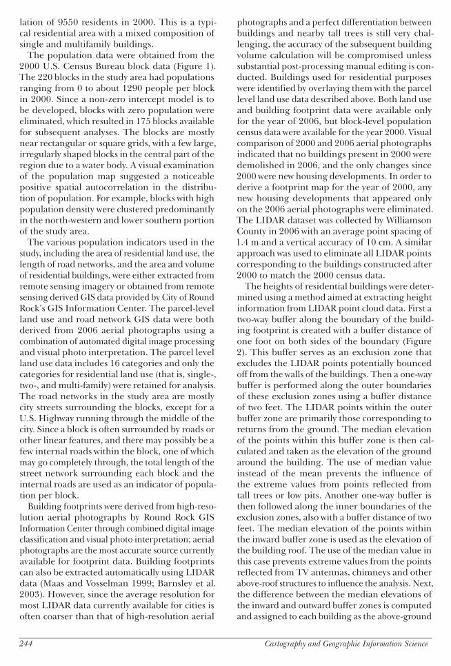
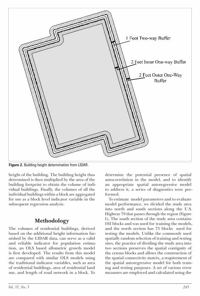
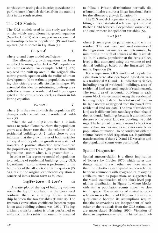
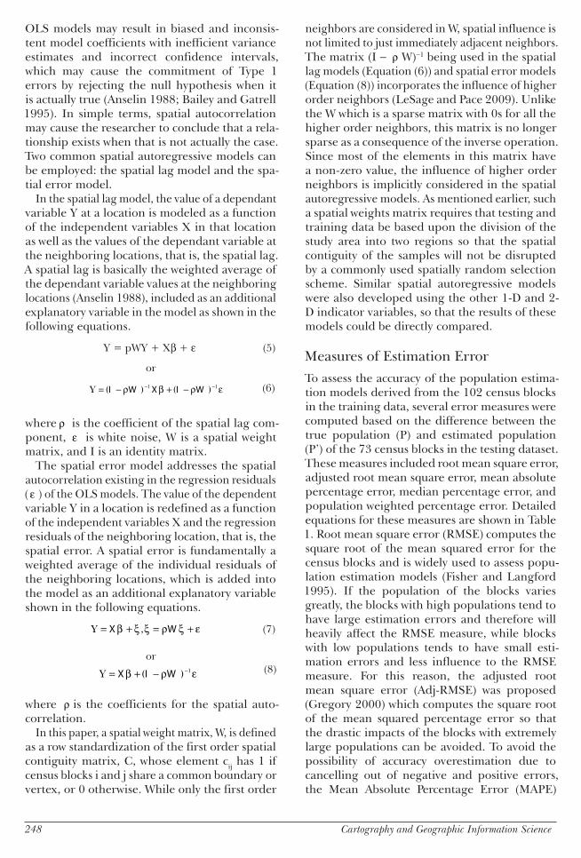
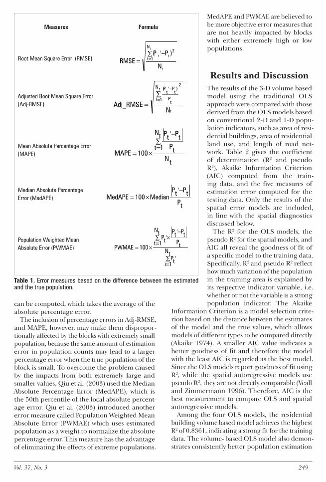
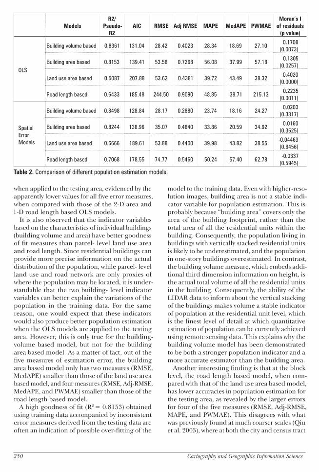
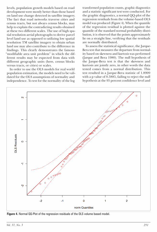
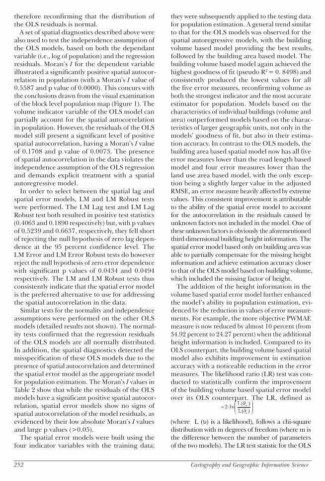
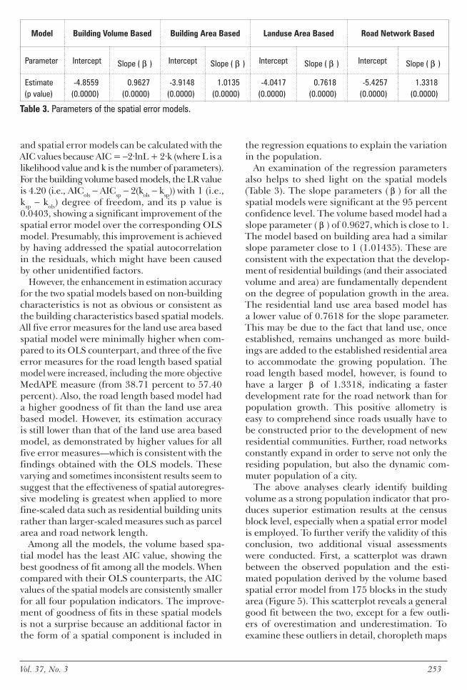


![Time-Varying Autoregressive Conditional Duration Model2.4 Autoregressive conditional duration model Engle and Russell [9] considered the autoregressive conditional duration (ACD) models](https://static.fdocuments.in/doc/165x107/61080978d0d2785210086daa/time-varying-autoregressive-conditional-duration-model-24-autoregressive-conditional.jpg)


