Estimation of Autoregressive with Exogeneous Inputs...

Estimation of Autoregressive with Exogeneous Inputs Model for

fMRI Data

Nattaporn Plub-in, Patawee Prakrankamanant, Nop PolboonRanyaphat Hongpipatsak, Morokot Cheat, Jitkomut Songsiri

Department of Electrical EngineeringFaculty of Engineering

Chulalongkorn University

November 21, 2016

Contents

1 Introduction 2

2 fMRI 32.1 Acquiring of fMRI data . . . . . . . . . . . . . . . . . . . . . . . . . . . . . . . . . . 32.2 Overview of ARX model . . . . . . . . . . . . . . . . . . . . . . . . . . . . . . . . . . 42.3 Granger Causality (GC) . . . . . . . . . . . . . . . . . . . . . . . . . . . . . . . . . . 6

3 Estimating formulation 83.1 ARX model with zero constraints . . . . . . . . . . . . . . . . . . . . . . . . . . . . . 83.2 The description of the data neuroimage (2013) . . . . . . . . . . . . . . . . . . . . . 9

4 Experiments 104.1 Preprocessing on fMRI data . . . . . . . . . . . . . . . . . . . . . . . . . . . . . . . 104.2 Least-square estimation of ARX models . . . . . . . . . . . . . . . . . . . . . . . . . 12

5 Conclusions 16

Appendices

A ARX model 18

B ARX with zero constraints 19

C Programming code 21C.1 The matlab code for finding the cardiac and respiratory signals . . . . . . . . . . . . 21C.2 Matlab code of ARX models . . . . . . . . . . . . . . . . . . . . . . . . . . . . . . . 22

1

Abstract

Functional Magnetic Resonance Imaging (fMRI) is one of the most popular methods tomeasure human brain activities. The fMRI based on BOLD effect describes the activated brainregion according to neuron activity in order to analyze brain connectivity. This study aimsto estimate the BOLD response using an autoegressive model with exogenous input (ARX). Aleast-square technique is applied to fit model. Since the AR coefficients have a joint zero patterndue to Granger causality, the results were generated by two models: ARX with unconstraint andARX with zero constraint. The results of this study presented the performance of two modelsusing the differrence between true data and estimated data. Finally, the accuracy of two modelswas discussed.

1 Introduction

Brain connectivity is one of the most popular topics of neuroscience. It is extremely challengingto explore how regions in brain communicate with each other since there no model truly explain-ing about brain connectivity. Nowadays, brain activity can be interpretted in different ways withdifferent methods such as electroencephalogram (EEG), magnetoencephalogram (MEG) and func-tional magnetic resonance imaging (fMRI). This project estimated brain connectivity by usingfMRI widely utilized for measuring brain function activity. fMRI is modified from magnetic res-onance imaging (MRI) [8] by using neuroimaging technology to generate 3D images of brain. Inaddition, it is also comfortable to be geometrically interpretted in term of 2D data by concerningthe Blood-oxygenation-level-dependent (BOLD) signals of each voxel.

This paper studies on brain connectivity estimation using ARX model studying from the previouspaper [11] using AR model and concerning Granger causality which is a statistical concept ofcausality that is based on prediction. According to this concept, if a signal yi is Granger-causedby a signal yj , then past values of yj helps predict furure values of yi more than only using pastvalues of yi.

This paper developes from the estimation brain connectivity in [11] stating that brain connectivityhas Granger causality properties. If the states at time series yi is Granger-caused by time series yj ,the past values of yj will help to improve the prediction of yi. [11] had estimated brain connectivityby autoregressive model with Granger causality properties as (1).

y(t) = A1y(t− 1) +A2y(t− 2) + · · ·+Apy(t− p) + u(t) (1)

where y(·) ∈ Rn, Ak ∈ Rnxn, k = 1, 2, . . . , p and u(·) is input noise.(we denote (Ak)ij the (i, j) entry of matrix Ak.)In this project, we add input variables into AR model from (1) then the model turn into autoregressive model with exogenous input (ARX) as (2).

y(t) =

p∑k=1

Aky(t− k) +

q∑k=1

Bku(t− k) + e(t) (2)

where y is the observed BOLD signal, u is controlled variables such as change in stimuli (visualcue or auditory signal) and e is noise.

We use ARX model because model with input variables can be estimated the brain connectivitymore precise by input variables are describe in section 3. A main goal of our project is analysisand simulations of ARX model can describe the brain connectivity with more precise and accuracy.The following section describes details of fMRI, the type of signals that we got from fMRI and thebasic concept of Granger causality. In section 3, we present overview of ARX model and estimationmethod including the description of data which we use in this project. In section 4, we describeexperiment and result of this work. Lastly, the conclusion will be discusses in section 5.

2

Figure 1: MRI Scannersource :

http://www.clipmass.com/story/35886

Figure 2: MR imagesource : https://pixabay.com/

2 fMRI

2.1 Acquiring of fMRI data

Magnetic resonance imaging (MRI) is a medical imaging technique used in radiology to form 3Dimages of the anatomy and the physiological processes of the body using MRI machine as shownin Figure 1. The brief principle is that MR scanner release radio wave to align Hydrogen atomsexisting within an interesting regions. When the energy are emitted back for returning to theresting state of atoms, the MR scanner captures this energy by the coils. Next, the computerprocesses the signals and generates a series of 2D grey-scaled images from the 3D image. As shownin Figure 2 is the example of MR image.

Functional magnetic resonance imaging (fMRI) modified from MRI is a medical imaging tech-nique which maps patterns of brain activation with high spatial resolution by measuring changes inblood. The fMRI bases on the BOLD effect consisting of the two fact. The first fact is that whenhemoglobin, the cell in blood that carries O2, loses O2 to become deoxyhemoglobin, the magneticproperties change. The sencond fact is that when an area of brain is activated, the blood flowincreases. These produce the BOLD effect, a local increase of the MR signal owing to a reductionof the oxygen extraction fraction during increased neural activity. An fMRI image shows the resultin term of 3D image. The 3D image is a volume resolution element as called voxel. Consideringeach voxel for all sampling time, the plot between the intensity of image in the voxel and time iscalled a BOLD signal shown in Figure 3.

The basis of most of the fMRI studies of brain activation performed today is BOLD signalsbased the fact that fully oxygenated blood has about the same susceptibility as other brain tissues,but deoxyhemoglobin is paramagnetic and changes the susceptibility of the blood. When regionsbecome more deoxygenated, field distortions around the vessels are increased by MRI machinedetection, and the BOLD signal decreases. On the contrary, if blood oxygenation increases, theBOLD signal also increases. That means deoxyhemoglobin has the effect of restraint the BOLDsignal, while oxyhemoglobin does not [8]. As shown in 4, the left figure illustrates a resting regionwhich has a small blood flow of both deoxyhemoglobin and oxyhemoglobin. Because of a smalldifference of blood susceptibility, BOLD signals are not affected much. In the contrary, the rightfigure illustrates a activated region. When a region is activated, a lot of oxygenated blood flowraises and then drops by becoming deoxygenated blood. Thus, when the region is activated, BOLD

3

http://www.clipmass.com/story/35886

https://pixabay.com/

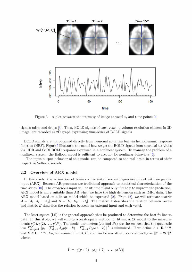
Figure 3: A plot between the intensity of image at voxel vi and time points [4]

signals raises and drops [3]. Then, BOLD signals of each voxel, a volumn resolution element in 3Dimage, are recorded as 2D graph expressing time-series of BOLD signals

BOLD signals are not obtained directly from neuronal activities but via hemodynamic responsefunction (HRF). Figure 5 illustrates the model how we get the BOLD signals from neuronal activitiesvia HDR and fMRI BOLD response expressed in a nonlinear system. To manage the problem of anonlinear system, the Balloon model is sufficient to account for nonlinear behaviors [5].

The input-output behavior of this model can be compared to the real brain in terms of theirrespective Volterra kernels.

2.2 Overview of ARX model

In this study, the estimation of brain connectivity uses autoregressive model with exogenousinput (ARX). Because AR processes are traditional approach to statistical characterization of thetime series [10]. The exogenous input will be utilized if and only if it help to improve the prediction.ARX model is more suitable than AR when we have the high demension such as fMRI data. TheARX model based on a linear model which be expressed (2). From (2), we will estimate matrixA = [A1 A2 . . . Ap] and B = [B1 B2 . . . Bq]. The matrix A describes the relation between voxelsand matrix B describes the relation between an external input and each voxel.

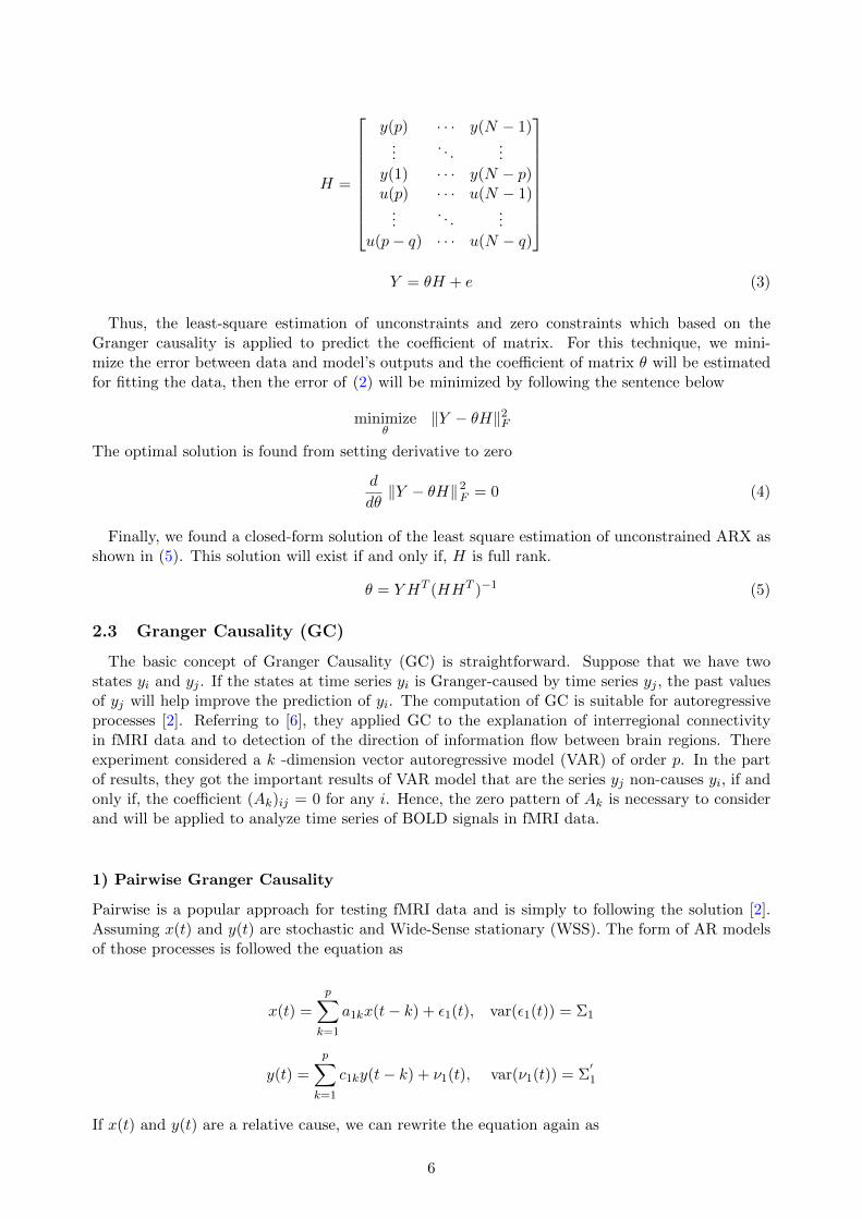
The least-square (LS) is the general approach that be produced to determine the best fit line todata. In this study, we will employ a least-square method for fitting ARX model to the measure-ments y(1), y(2), . . . , y(N). The model parameters (Ak and Bk) are chosen such that the quadraticloss

∑Nt=p+1 ‖yt −

∑pk=1Aky(t− k)−

∑qk=1Bku(t− k)‖2 is minimized. If we define A ∈ R n×np

and B ∈ R n×mq. So, we assume θ = [A B] and can be rewritten more compactly as ‖Y − θH‖22where

Y =[y(p+ 1) y(p+ 2) . . . y(N)

]4

Figure 4: Illustration of the BOLD mechanism. During activated periods, the blood flow increasesand more oxygenated than resting then, the location of neronal activies are found.

source : http://www.sbirc.ed.ac.uk/research/techniques/functional.html

Figure 5: The BOLD signal has several constituents: (1) the neuronal response to a stimulus orbackground modulation; (2) the complex relationship between neuronal activity and triggering ahaemodynamic response (termed neurovascular coupling); (3) the haemodynamic response itself;and (4) the way in which this response is detected by an MRI scanner [1].

5

http://www.sbirc.ed.ac.uk/research/techniques/functional.html

H =

y(p) · · · y(N − 1)...

. . ....

y(1) · · · y(N − p)u(p) · · · u(N − 1)

.... . .

...u(p− q) · · · u(N − q)

Y = θH + e (3)

Thus, the least-square estimation of unconstraints and zero constraints which based on theGranger causality is applied to predict the coefficient of matrix. For this technique, we mini-mize the error between data and model’s outputs and the coefficient of matrix θ will be estimatedfor fitting the data, then the error of (2) will be minimized by following the sentence below

minimizeθ

‖Y − θH‖2F

The optimal solution is found from setting derivative to zero

d

dθ‖Y − θH‖2F = 0 (4)

Finally, we found a closed-form solution of the least square estimation of unconstrained ARX asshown in (5). This solution will exist if and only if, H is full rank.

θ = Y HT (HHT )−1 (5)

2.3 Granger Causality (GC)

The basic concept of Granger Causality (GC) is straightforward. Suppose that we have twostates yi and yj . If the states at time series yi is Granger-caused by time series yj , the past valuesof yj will help improve the prediction of yi. The computation of GC is suitable for autoregressiveprocesses [2]. Referring to [6], they applied GC to the explanation of interregional connectivityin fMRI data and to detection of the direction of information flow between brain regions. Thereexperiment considered a k -dimension vector autoregressive model (VAR) of order p. In the partof results, they got the important results of VAR model that are the series yj non-causes yi, if andonly if, the coefficient (Ak)ij = 0 for any i. Hence, the zero pattern of Ak is necessary to considerand will be applied to analyze time series of BOLD signals in fMRI data.

1) Pairwise Granger Causality

Pairwise is a popular approach for testing fMRI data and is simply to following the solution [2].Assuming x(t) and y(t) are stochastic and Wide-Sense stationary (WSS). The form of AR modelsof those processes is followed the equation as

x(t) =

p∑k=1

a1kx(t− k) + ε1(t), var(ε1(t)) = Σ1

y(t) =

p∑k=1

c1ky(t− k) + ν1(t), var(ν1(t)) = Σ′1

If x(t) and y(t) are a relative cause, we can rewrite the equation again as

6

x(t) =

p∑k=1

a2kx(t− k) +

p∑k=1

c′2ky(t− k) + ε2(t) (6)

y(t) =

p∑k=1

c2ky(t− k) +

p∑k=1

a′2kx(t− k) + ν2(t) (7)

Then, we define q(t) =

[x(t)y(t)

]=∑p

k=1Hkq(t− k) + γ(t) and the covariance matrix of noise is var

(γ(t)) =

[Σ2 TT T Σ

′2

]i.e., var(ε2(t)) = Σ2, var(ν2(t)) = Σ

′2 and T = cov(ε2(t), ν2(t))

If x(t) and y(t) are independent, c2 and c′2 are zero. We can say that T is zero.

From [2], we can find the quantity of y(t) which is a Granger-cause on x(t) as

Fy→x = lnΣ1

Σ2

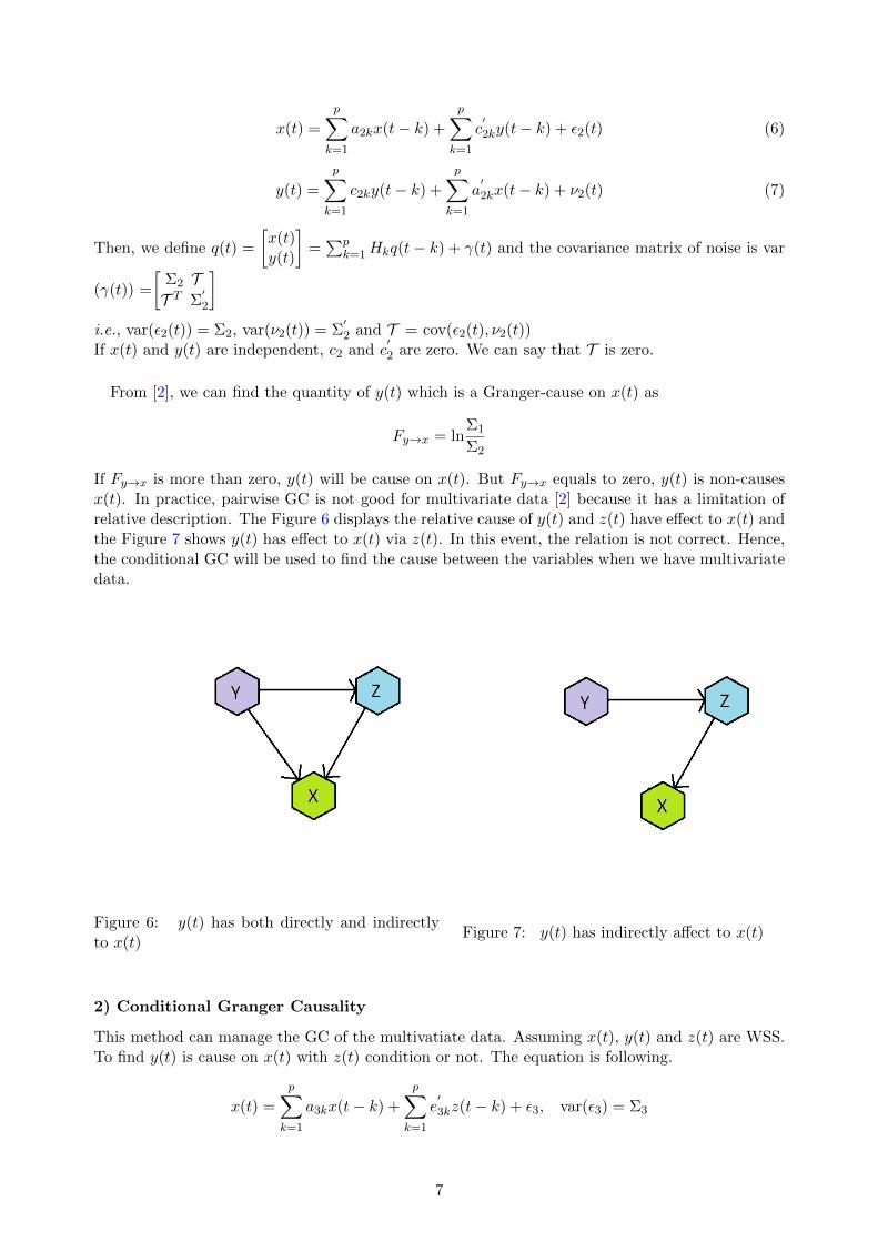
If Fy→x is more than zero, y(t) will be cause on x(t). But Fy→x equals to zero, y(t) is non-causesx(t). In practice, pairwise GC is not good for multivariate data [2] because it has a limitation ofrelative description. The Figure 6 displays the relative cause of y(t) and z(t) have effect to x(t) andthe Figure 7 shows y(t) has effect to x(t) via z(t). In this event, the relation is not correct. Hence,the conditional GC will be used to find the cause between the variables when we have multivariatedata.

Figure 6: y(t) has both directly and indirectlyto x(t)

Figure 7: y(t) has indirectly affect to x(t)

2) Conditional Granger Causality

This method can manage the GC of the multivatiate data. Assuming x(t), y(t) and z(t) are WSS.To find y(t) is cause on x(t) with z(t) condition or not. The equation is following.

x(t) =

p∑k=1

a3kx(t− k) +

p∑k=1

e′3kz(t− k) + ε3, var(ε3) = Σ3

7

z(t) =

p∑k=1

e′3kz(t− k) +

p∑k=1

a3kx(t− k) + ν3, var(ν3) = Σ′3

Then, the covariance matrix of noise between x(t) and z(t) are defined as Σ =

[Σ3 TT T Σ

′3

]If x(t), y(t) and z(t) are a relative cause, we can rewrite the equation again as

x(t) =

p∑k=1

a4kx(t− k) +

p∑k=1

c′4ky(t− k) +

p∑k=1

e′4kz(t− k) + ε4 (8)

y(t) =

p∑k=1

a∗4kx(t− k) +

p∑k=1

c4ky(t− k) +

p∑k=1

e∗4kz(t− k) + ν4 (9)

z(t) =

p∑k=1

a′4kx(t− k) +

p∑k=1

c∗4ky(t− k) +

p∑k=1

e4kz(t− k) + λ4 (10)

We define the covariance matrix of noise as Σ=

Σxx Σxy Σxz

Σyx Σyy Σyz

Σzx Σzy Σzz

Look like the pairwise method to

find the quantity of y(t) is cause on x(t) with z(t) condition as shown below :

Fy→x|z = lnΣ3

Σxx

We found that if Fy→x|z is more than zero, y(t) will be cause on x(t) with z(t) condition. In otherword, if Σ3 =Σxx, Fy→x|z equals to zero. So, y(t) is not cause on x(t) with z(t) condition.

Both of pairwise and conditional GC can lead to the zero pattern of Ak. If y(t) is not directcause on x(t), the coefficient will be zero. i.e., the some element of (Ak)ij is zero. For fMRI datasets, the conditional GC is more appropriate than pairwise GC since we can set the other voxelsthat are not interest to be the conditional terms.

3 Estimating formulation

In this section, we present the formulation for finding the brian connectivity. i.e., A and B willbe estimated using ARX both with and without constraints. The ARX with zero constraints willbe explained as a straigthforward way. After that, the details of data neuroimage(2013) from [7]will be described how we get BOLD signals.

3.1 ARX model with zero constraints

If the Granger Causality is given, the problem of estimating ARX model subjects to zero con-straint (i.e a brain network topology is known and our data contains the zero pattern of Ak).

Next, we will define the new term of matrix below

Y = [y1 y2 . . . yN ] where Y ∈ R n×N

A = [A1 A2 . . . Ap] where A ∈ R n×np and Ak ∈ R n×n for k = 1, 2, . . . , p

B = [B1 B2 . . . Bq] where B ∈ R n×mq and Bk ∈ R n×m for k = 1, 2, . . . , q

where n is a number of voxel in brain, N is a number of measurement and p is the index ofGranger causality data (the position that we know the data is Granger).

8

By then, we define

H =

y(p) · · · y(N − 1)...

. . ....

y(1) · · · y(N − p)

=

H1...Hp

and K =

u(p) · · · u(N − 1)...

. . ....

u(p− q) · · · (N − q)

=

K1...Kq

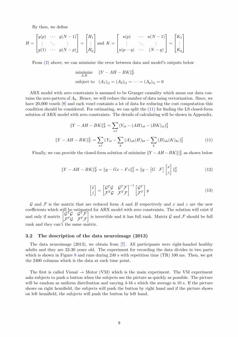
From (2) above, we can minimize the error between data and model's outputs below

minimizeA,B

‖Y −AH −BK‖2F

subject to (A1)ij = (A2)ij = · · · = (Ap)ij = 0

ARX model with zero constraints is assumed to be Granger causality which mean our data con-tains the zero pattern of Ak. Hence, we will reduce the number of data using vectorization. Since, wehave 20,000 voxels [8] and each voxel containts a lot of data for reducing the cost computation thiscondition should be considered. For estimating, we can split the (11) for finding the LS closed-formsolution of ARX model with zero constraints. The details of calculating will be shown in Appendix.

‖Y −AH −BK‖2F =∑s,t

(Yst − (AH)st − (BK)st)22

‖Y −AH −BK‖2F =∑s,t

(Yst −∑k

(A)sk(H)kt −∑k

(B)sk(K)kt )22 (11)

Finally, we can provide the closed-form solution of minimize ‖Y −AH−BK‖|2F as shown below

‖Y −AH −BK‖2F = ‖y −Gx− Fz‖22 = ‖y −[G F

] [xz

]‖22 (12)

[xz

]=

[GTG GTFFTG FTF

]−1 [GTFT]y (13)

G and F is the matrix that are reduced form A and B respectively and x and z are the newcoefficients which will be estimated for ARX model with zero constraints. The solution will exist if

and only if matrix

[GTG GTFFTG FTF

]is invertible and it has full rank. Matrix G and F should be full

rank and they can’t the same matrix.

3.2 The description of the data neuroimage (2013)

The data neuroimage (2013), we obtain from [7]. All participants were right-handed healthyadults and they are 22-30 years old. The experiment for recording the data divides in two partswhich is shown in Figure 8 and runs during 240 s with repetition time (TR) 100 ms. Then, we gotthe 2400 columns which is the data at each time point.

The first is called Visual → Motor (VM) which is the main experiment. The VM experimentasks subjects to push a button when the subjects see the picture as quickly as possible. The picturewill be random as uniform distribution and varying 4-16 s which the average is 10 s. If the pictureshows on right hemifield, the subjects will push the button by right hand and if the picture showson left hemifield, the subjects will push the button by left hand.

9

The second is called Motor→ Visual (MV) which is the control experiment. The MV experimentasks subjects to push a button after hearing a 200 ms tone pip at the differential frequency as 1kHz for left hand and 4 kHz for right hand. The tone pip is defined to be uniform distribution andvarying 4-16 s which the average is 10 s like VM experiment. After the subjects push the button,the picture will display the same side as the subjects push the button by hand side. The latencybetween the button press and the onset of visual stimulation was 158 ms for the right and 220 msfor the left hand. This experiment is designed to check VM experiment in term of the oppositeway. In the VM experiment, visual cortex works before motor cortex but motor cortex works beforevisual cortex for the MV experiment.

An exogenous input is included only for improving the prediction and control of some importantparameter if and only if the exogenous input is known and will be useful for the prediction [9].Then, ARX models are more suitable for fitting the data than AR models. This innovation is alsohelpful for characterization of the time series which is a very high dimension such as fMRI datawhose obtains from [7]. So, ARX models are applied to estimate the effective connectivity of humanbrain in our experiments.

In data set of VM experiment in neuroimage (2013), exogenous inputs come from condition ofvisual stimuli. The value equals to ”1” if the input stimuli shows left visual hemifield. The valueequals to 2’ if the input stimuli shows right visual hemifield. Otherwise, the value is ”0” whenthere is no any stimulus. We will decompose exogenous input into two dimension for left andright hemifield (u ∈ R2). Since timing of each visual stimulus was randomized with a uniformdistribution of interstimulus intervals (ISIs) varying from 4 to 16s (mean 10s) [7], it seems thatinputs are pseudo random sequences in estimation. For left hemifield input, it is random sequencesof unit interval [0,1]. The intervals are zero except intervals that show left visual stimuli equals to”1”. For right hemifield input, it is random sequences of interval [0,2]. Other intervals are zeroexcept intervals that show right visual stimuli equal to ”2”. Similar to VM experiment, exogenousinputs of MV experiment are two dimensions on condition of left or right hand push the button.They were presented randomly too. Therefore, we will use these exogenous input for our ARXmodel.

4 Experiments

4.1 Preprocessing on fMRI data

In this experiment, we try to remove the noise of BOLD signals. The BOLD signal in fMRI datareflects both neuronal activations and global physiological fluctuations. The main physiologicalprocesses seen in BOLD data are physiological low frequency oscillations, respiration, and cardiacpulsation. These different physiological processes confound the BOLD signals in different ways.The high frequency physiological signals (i.e., from respiration and cardiac pulsation) are aliasedinto the low frequency band, making it hard to study the individual effect of these physiologicalprocesses on BOLD signal. Thus, we use the spectral method to find the reference signals.

Spectral method try to remove different physiological signals from BOLD signal, the power spec-trum of BOLD signal at each voxel was calculated for each participant. Without external referencesignal, its difficult to accurately estimate cardiac and respiratory cycles. However, we consider tosearch all time series for the one with the highest percentage of power spectra density between 0.8Hz and 1.5 Hz as a ”pseudo cardiac signal and the one with the highest percentage power between0.16 Hz and 0.3 Hz as a pseudo respiratory signal. We consider this time series is pseudo cardiacor respiratory signal which influenced by BOLD signal. This experiment we use DRIFTER matlabtoolbox which downloads from http://becs.aalto.fi/en/research/bayes/drifter/.

10

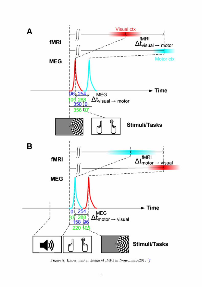
http://becs.aalto.fi/en/research/bayes/drifter/

Figure 8: Experimental design of fMRI in NeuroImage2013 [7]

11

0 50 100 150 200 2500.88

0.9

0.92

0.94

Time [s]

Results

Observed data

Estimate

0 50 100 150 200 2500.02

0.03

0.04

0.05Cardiac reference signal

Time [s]

0 50 100 150 200 250−5

0

5

10x 10

−3 Cardiac signal Estimate

Time [s]

0 50 100 150 200 25040

60

80

100Cardiac signal Frequency

Time [s]

Fre

q (

bpm

)

0 50 100 150 200 2500.02

0.03

0.04

0.05Respiratory reference signal

Time [s]

0 50 100 150 200 250−0.01

−0.005

0

0.005

0.01Respiratory signal Estimate

Time [s]

0 50 100 150 200 2505

10

15

20Respiratory signal Frequency

Time [s]

Fre

q (

bpm

)Figure 9: The example data of observed data and estimate data after remove cardiac and respiratorysignals

1 2 3 4 5 6 7 8 9−4000

−3000

−2000

−1000

0

1000

2000AIC unconstrain

p

AIC

score

q=1

q=2

q=3

AIC with noise variance 0.5

1 2 3 4 5 6 7 8 90

0.5

1

1.5

2

2.5x 10

4 AIC unconstrain

p

AIC

score

q=1

q=2

q=3


1 2 3 4 5 6 7 8 90

0.5

1

1.5

2

2.5

3

3.5

4

4.5x 10

4 AIC unconstrain

p

AIC

score

q=1

q=2

q=3


Figure 10: Bar graphs present AIC of ARX unconstraint with dense A.

The SPM toolbox is an implement of the DRIFTER algorithm, which is a Bayesian method forphysiological noise modeling and removal allowing accurate dynamical tracking of the variationsin the cardiac and respiratory frequencies by using Interacting Multiple Models (IMM), KalmanFiler (KF) and Rauch-Tung-Striebel (RTS) smoother algorithms. The result from this trial will beshown in Figure 9 which the example of fMRI data run into SPM toolbox for finding the cardiacand respiratory signals. After finished this process, we will get the clean BOLD signals from fMRIdata sets and will be used to do the next experiment.

4.2 Least-square estimation of ARX models

Experiment of model selection by AIC and BIC

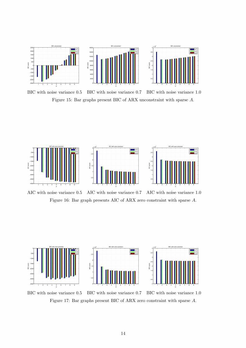
The experiment started from generating data with order p = 4 and q = 2 and finding AIC andBIC values of all possible pairs of p, q for indicating which orders have a good fitting on ARXmodel. This experiment aims to examine whether AIC and BIC were able to choose the correctcasual orders, p = 4 and q = 2 while varying noise variance and density of matrix A.

From the above results, we saw that each q are scanty affected in AIC and BIC value becausethe large number of measured data y are dominant over the small number of input u. For eachq, the AIC and BIC values significantly varied when p = 1 to 4. For p more than 4, they slightly

12

1 2 3 4 5 6 7 8 9−2000

−1500

−1000

−500

0

500

1000

1500

2000

2500BIC unconstrain

p

BIC

score

q=1

q=2

q=3

BIC with noise variance 0.5

1 2 3 4 5 6 7 8 90

0.5

1

1.5

2

2.5x 10

4 BIC unconstrain

p

BIC

score

q=1

q=2

q=3


1 2 3 4 5 6 7 8 90

0.5

1

1.5

2

2.5

3

3.5

4

4.5x 10

4 BIC unconstrain

p

BIC

score

q=1

q=2

q=3


Figure 11: Bar graphs present BIC of ARX unconstraint with dense A.

1 2 3 4 5 6 7 8 9−4000

−3000

−2000

−1000

0

1000

2000

3000AIC with zero constrain

p

AIC

score

q=1

q=2

q=3


1 2 3 4 5 6 7 8 90

0.5

1

1.5

2

2.5

3x 10

4 AIC with zero constrain

p

AIC

score

q=1

q=2

q=3


1 2 3 4 5 6 7 8 90

0.5

1

1.5

2

2.5

3

3.5

4

4.5x 10


pA

IC s

core

q=1

q=2

q=3


Figure 12: Bar graph presents AIC of ARX zero constraint with dense A.

1 2 3 4 5 6 7 8 9−2500

−2000

−1500

−1000

−500

0

500

1000

1500

2000

2500BIC with zero constrain

p

BIC

score

q=1

q=2

q=3


1 2 3 4 5 6 7 8 90

0.5

1

1.5

2

2.5

3x 10

4 BIC with zero constrain

p

BIC

score

q=1

q=2

q=3


1 2 3 4 5 6 7 8 90

0.5

1

1.5

2

2.5

3

3.5

4

4.5x 10


p

BIC

score

q=1

q=2

q=3


Figure 13: Bar graphs present BIC of ARX zero constraint with dense A.

1 2 3 4 5 6 7 8 9−4000

−3500

−3000

−2500

−2000

−1500

−1000

−500

0AIC unconstrain

p

AIC

sco

re

q=1

q=2

q=3


1 2 3 4 5 6 7 8 90

2000

4000

6000

8000

10000

12000

14000AIC unconstrain

p

AIC

score

q=1

q=2

q=3


1 2 3 4 5 6 7 8 90

0.5

1

1.5

2

2.5

3

3.5x 10

4 AIC unconstrain

p

AIC

score

q=1

q=2

q=3


Figure 14: Bar graphs present AIC of ARX unconstraint with sparse A.

13

1 2 3 4 5 6 7 8 9−2500

−2000

−1500

−1000

−500

0

500

1000

1500

2000

2500BIC unconstrain

p

BIC

sco

re

q=1

q=2

q=3


1 2 3 4 5 6 7 8 90

2000

4000

6000

8000

10000

12000

14000

16000BIC unconstrain

pB

IC s

core

q=1

q=2

q=3


1 2 3 4 5 6 7 8 90

0.5

1

1.5

2

2.5

3

3.5

4x 10

4 BIC unconstrain

p

BIC

score

q=1

q=2

q=3


Figure 15: Bar graphs present BIC of ARX unconstraint with sparse A.

1 2 3 4 5 6 7 8 9−4000

−3500

−3000

−2500

−2000

−1500

−1000

−500

0AIC with zero constrain

p

AIC

sco

re

q=1

q=2

q=3


1 2 3 4 5 6 7 8 90

0.5

1

1.5

2

2.5

3x 10


p

AIC

score

q=1

q=2

q=3


1 2 3 4 5 6 7 8 90

0.5

1

1.5

2

2.5

3

3.5

4x 10


p

AIC

score

q=1

q=2

q=3


Figure 16: Bar graph presents AIC of ARX zero constraint with sparse A.

1 2 3 4 5 6 7 8 9−3500

−3000

−2500

−2000

−1500

−1000

−500

0BIC with zero constrain

p

BIC

sco

re

q=1

q=2

q=3


1 2 3 4 5 6 7 8 90

0.5

1

1.5

2

2.5

3x 10


p

BIC

score

q=1

q=2

q=3


1 2 3 4 5 6 7 8 90

0.5

1

1.5

2

2.5

3

3.5

4x 10


p

BIC

score

q=1

q=2

q=3


Figure 17: Bar graphs present BIC of ARX zero constraint with sparse A.

14

zc with N(0,0.1) uc with N(0,0.1) zc with N(0,0.5) uc with N(0,0.5) zc with N(0,0.7) uc with N(0,0.7) zc with N(0,1) uc with N(0,1)

50

100

150

200

250

300

350

Bou

nde

d o

f e

rro

r w

ith

100d

ata

sets

Figure 18: The norm error of 100 data sets which is generated with noise variance equals toN (0, 0.1), N (0, 0.5), N (0, 0.7), and N (0, 1) at p = 4, q = 2 and N = 2400 where the red linedisplays the median values of data sets, horizontal black line displays the bounds of data sets, bluebox contains 50% of middle data sets, below vertical dash line displays 25% of the first data respectto the quartiles of a ranked set, above vertical dash line displays 25% of the last data and red crossdisplays outlier point.

varied. The casual order p = 4 and q =1 are chosen as the mode of order giving the least AIC andBIC value for each table.

Experiment of random data for testing the estimation with different noise vari-ance

For the section of experiment, we generate the random data for testing the estimation of ourARX models. With writing our code of ARX model, we produce the experiment on our model byestimation of data which is generated in MATLAB via random data. The random data is definedto be normal distribution with zero mean and variance is varied to be 0.1, 0.5, 0.7 and 1. Therandom data that we generate is y ∈ R10 and u ∈ R2 and is defined to be stationary by giventhe condition. The random data sets is generated to be 100 and 200 data sets. The results of thisexperiments descibe the performance of estimation by our models. The details of MATLAB codethat we use to find the results will be shown in Appendix.

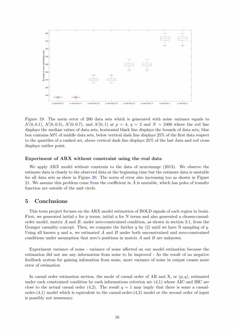
To show the performance between models, the 100 and 200 data sets of y are generated withnoise of variance which has been varied distribution as N (0, 0.1), N (0, 0.5), N (0, 0.7) and N (0, 1).With our assumption, if y is generated with high noise variance, the error between y and yest willbe much more than y with small noise variance. To verify the assumption, the comparison of normerror is produced with difference noise variance. The data sets contain 2400 samplings ( N = 2400).As shown in 18 and 19 are the comparison of norm error which is presented by box plot.

The results of our experiments can conclude that the noise variance has affected to estimationof both techniques. As shown in the Figure 18 and 19 can conclude that the noise variance equalsto 1 has higher values of bounded error than others. Likewise, y data sets with noise variance 0.7,0.5 and 0.1 have the values of bounded error respective decrease.

15

zc with N(0,0.1) uc with N(0,0.1) zc with N(0,0.5) uc with N(0,0.5) zc with N(0,0.7) uc with N(0,0.7) zc with N(0,1) uc with N(0,1)

200

220

240

260

280

300

320

340

360

Bou

nde

d o

f e

rro

r w

ith

200d

ata

sets

Figure 19: The norm error of 200 data sets which is generated with noise variance equals toN (0, 0.1), N (0, 0.5), N (0, 0.7), and N (0, 1) at p = 4, q = 2 and N = 2400 where the red linedisplays the median values of data sets, horizontal black line displays the bounds of data sets, bluebox contains 50% of middle data sets, below vertical dash line displays 25% of the first data respectto the quartiles of a ranked set, above vertical dash line displays 25% of the last data and red crossdisplays outlier point.

Experiment of ARX without constraint using the real data

We apply ARX model without constrain to the data of neuroimage (2013). We observe theestimate data is closely to the observed data at the beginning time but the estimate data is unstablefor all data sets as show in Figure 20. The norm of error also increasing too as shown in Figure21. We assume this problem come from the coefficient in A is unstable, which has poles of transferfunction are outside of the unit circle.

5 Conclusions

This term project focuses on the ARX model estimation of BOLD signals of each region in brain.First, we generated initial y for p terms, initial u for N terms and also generated a chosen-casual-order model, matrix A and B, under zero-constrained condition, as shown in section 3.1, from theGranger casuality concept. Then, we compute the further y by (2) until we have N sampling of y.Using all known y and u, we estimated A and B under both unconstrained and zero-constrainedconditions under assumption that zero’s positions in matrix A and B are unknown.

Experiment variance of noise - variance of noise affected on our model estimation because theestimation did not use any information from noise to be improved - As the result of no negativefeedback system for gaining infomation from noise, more variance of noise in output causes moreerror of estimation

In casual order estimation section, the mode of casual order of AR and X, or (p, q), estimatedunder each constrained condition by each informations criterion are (4,1) whose AIC and BIC areclose to the actual casual order (4,2). The result q = 1 may imply that there is some a casual-order-(4,1) model which is equivalent to the casual-order-(4,2) model or the second order of inputis possibly not nessessary.

16

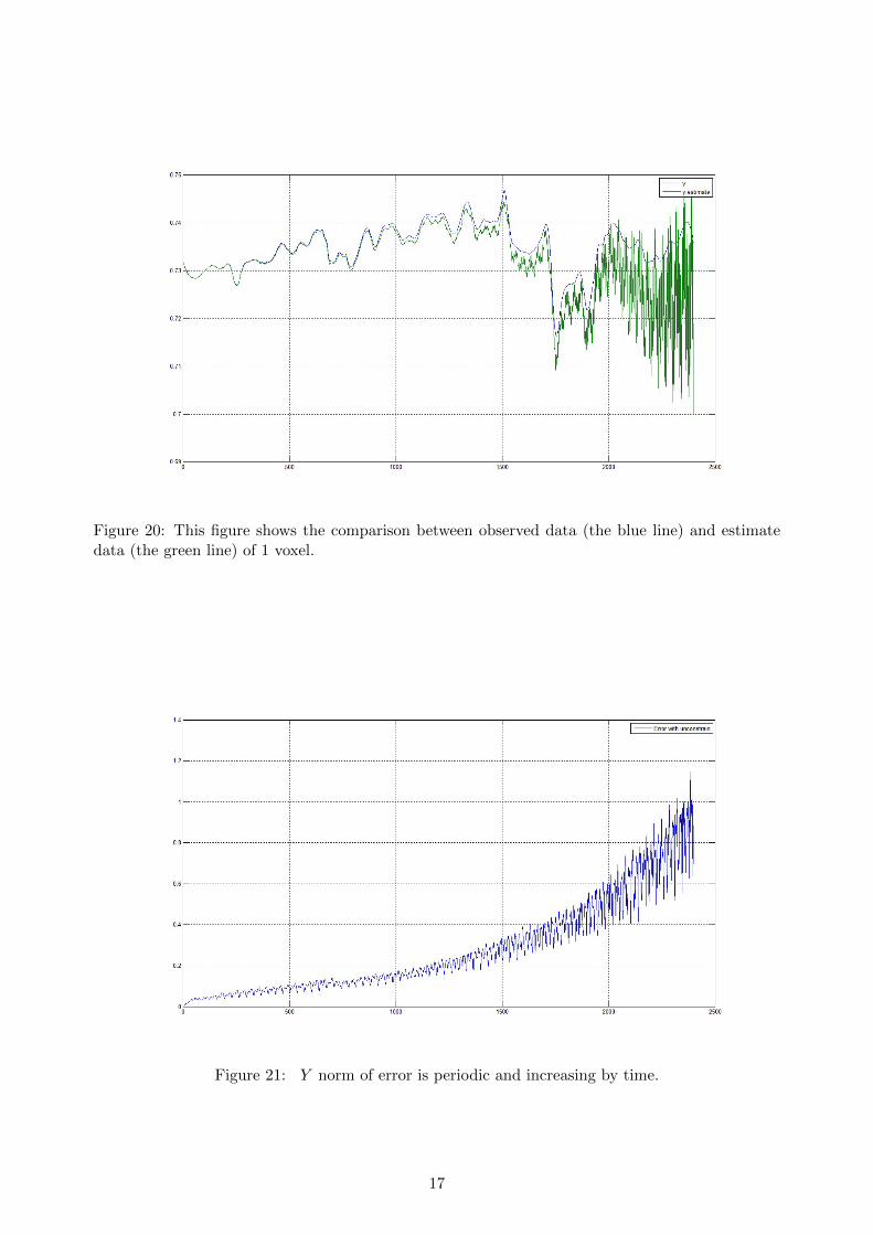
Figure 20: This figure shows the comparison between observed data (the blue line) and estimatedata (the green line) of 1 voxel.

Figure 21: Y norm of error is periodic and increasing by time.

17

Lastly, we prepared the real fMRI data for estimation by removing respiratory and cardiac noisein section 4.1 and illustrated of using real data for estimation in section 4.2.

References

[1] Owen J Arthurs and Simon Boniface. How well do we understand the neural origins of thefMRI BOLD signal? Trends in neurosciences, 25(1):27–31, 2002.

[2] Steven L Bressler and Anil K Seth. Wiener–Granger causality: a well established methodology.Neuroimage, 58(2):323–329, 2011.

[3] Richard B. Buxton. In Introduction to Functional Magnetic Resonance Imaging Principles andTechniques, pages 110–111. Cambridge, 2009.

[4] Ani Eloyan, Shanshan Li, John Muschelli, Jim J Pekar, Stewart H Mostofsky, and Brian SCaffo. Analytic programming with fMRI data: A Quick-start guide for statisticians using R.PloS one, 9(2):e89470, 2014.

[5] Karl J Friston, Andrea Mechelli, Robert Turner, and Cathy J Price. Nonlinear responses infMRI: the Balloon model, Volterra kernels, and other hemodynamics. NeuroImage, 12(4):466–477, 2000.

[6] Rainer Goebel, Alard Roebroeck, Dae-Shik Kim, and Elia Formisano. Investigating directedcortical interactions in time-resolved fMRI data using vector autoregressive modeling andGranger causality mapping. Magnetic resonance imaging, 21(10):1251–1261, 2003.

[7] Fa-Hsuan Lin, Thomas Witzel, Tommi Raij, Jyrki Ahveninen, Kevin Wen-Kai Tsai, Yin-HuaChu, Wei-Tang Chang, Aapo Nummenmaa, Jonathan R Polimeni, Wen-Jui Kuo, et al. fMRIhemodynamics accurately reflects neuronal timing in the human brain measured by MEG.Neuroimage, 78:372–384, 2013.

[8] Martin A Lindquist et al. The Statistical analysis of fMRI data. Statistical Science, 23(4):439–464, 2008.

[9] Tohru Ozaki. Time series modeling of neuroscience data. CRC Press, 2012.

[10] Tata Subba Rao, Suhasini Subba Rao, and Calyampudi Radhakrishna Rao. Handbook ofstatistics: time series analysis: methods and applications, volume 30. Elsevier, 2012.

[11] Jitkomut Songsiri. Sparse autoregressive model estimation for learning granger causality intime series. In 2013 IEEE International Conference on Acoustics, Speech and Signal Processing,pages 3198–3202. IEEE, 2013.

Appendices

A ARX model

In this section, we want to extend why we get ‖Y − θH‖2F as (3).

[y(p+ 1) · · · y(N)

]=[A1 · · · Ap B1 · · · BP

]

y(p) · · · y(N − 1)...

. . ....

y(1) · · · y(N − p)u(p) · · · u(N − 1)

.... . .

...u(p− q) · · · u(N − q)

+[e(p+ 1) · · · e(N)

]

18

Y = θH + e (14)

B ARX with zero constraints

From (11), we want to minimize ‖Y − AH − BK‖|2F . Then, vectorization is used to reduce thenumber of data and form a new matrix for replacing the summation term as shown below

‖Y −AH −BK‖|2F =∑s,t

(Yst − (AH)st − (BK)st)22

=∑s,t

(Yst −np∑k=1

(A)sk(H)kt −mq∑k=1

(B)sk(K)kt)22

A =[A1 A2 · · · AP

]∈ IRn×np where Ai ∈ IRn×n, (i = 1, 2, · · · , p)

B =[B1 B2 · · · Bq

]∈ IRn×mq where Bi ∈ IRn×m, (i = 1, 2, · · · , q)

H =

H1

H2...Hp

∈ IRnp×N where Hi ∈ IRn×N , (i = 1, 2, · · · , p)

K =

K1

K2...Kq

∈ IRmq×N where Ki ∈ IRm×N , (i = 1, 2, · · · , q)

np∑k=1

(A)sk(H)kt =

n∑k=1

[(H1)kt (H2)kt · · · (Hp)kt

]

(A1)sk(A2)sk

...(Ap)sk

=n∑k=1

Hk,tXsk

mq∑k=1

(B)sk(K)kt =

m∑k=1

[(K1)kt (K2)kt · · · (Kq)kt

]

(B1)sk(B2)sk

...(Bq)sk

=

m∑k=1

Kk,tZsk

⇒ YS,1YS,2

...Ys,N

=

H1,1 H1,2 · · · H1,n

H2,1 H2,2 · · · H2,n...

.... . .

...HN,1 HN,2 · · · HN,n

Xs,1

Xs,2...

Xs,n

+

K1,1 K1,2 · · · K1,m

K2,1 K2,2 · · · K2,m...

.... . .

...KN,1 KN,2 · · · KN,m

Zs,1Zs,2

...Zs,m

H =

H1,1 H1,2 · · · H1,n

H2,1 H2,2 · · · H2,n...

.... . .

...HN,1 HN,2 · · · HN,n

,K =

K1,1 K1,2 · · · K1,m

K2,1 K2,2 · · · K2,m...

.... . .

...KN,1 KN,2 · · · KN,m

⇒

Y1,2...

Y1,NY2,1

...Yn,N

= (In ⊗H)

X1,1...

X1,n

X2,1...

Xn,n

+ (In ⊗K)

Z1,1...

Z1,n

Z2,1...

Zn,n

19

G = In ⊗H, F = In ⊗K

⇒ We got,

‖Y −AH −BK‖2F = ‖y −Gx− Fz‖22 (15)

= ‖y −[G F

] [xz

]‖2

2

(16)[xz

]=

[GTG GTFFTG FTF

]−1 [GTFT]y (17)

20

C Programming code

C.1 The matlab code for finding the cardiac and respiratory signals

This part is a matlab code for finding the cardiac and respiratory signals from fMRI data sets usingDRIFTER toolbox. This is available download from http://becs.aalto.fi/en/research/bayes/

drifter/.

%Obtain the periodogram using fft. The signal is real-valued and has odd length.

%Because the signal is real-valued, you only need power estimates for the positive or negative frequencies.

%In order to conserve the total power,

%multiply all frequencies that occur in both sets the positive and negative frequencies by a factor of 2.

%Zero frequency (DC) and the Nyquist frequency do not occur twice.

load KuoPC_mv_02.mat;

%Load data(data contains data.voxels and data.input)

rawdata = KuoPC_mv_02.voxels;

N = 2399; %number of time points

T = linspace(0,240,N);

resp_max = 0;

card_max = 0;

for i = 1:length(rawdata)

%----------------- power spetra of time series ---------------------

x = rawdata(i,:);

N = length(x);

Fs = 1/(T(2)-T(1));

xdft = fft(x);

xdft1 = xdft(1:N/2+1);

psdx = (1/(2*pi*N)) * abs(xdft1).^2; %energy spectral density

psdx(2:end-1) = 2*psdx(2:end-1);

freq = 0:Fs/length(x):Fs/2;

%---------------------------------------------------------------

%--------------------- find graph area --------------------------

power = 0;

resp = 0;

card = 0;

for j = 1:(N/2+1)

%consider only positive freq and zero freq do not occur twice

freq_sam = freq(j+1)-freq(j);

power = power + (freq_sam*(psdx(j)+psdx(j+1))/2);

%freq range from 0.16 to 0.3 consider as a respiratory signals

if (0.16 < freq(j) && freq(j) <= 0.3)

resp = resp + (freq_sam*(psdx(j)+psdx(j+1))/2);

%freq range from 0.8 to 1.5 consider as a cardiac signals

elseif (0.8 < freq(j) && freq(j) <= 1.5)

card = card + (freq_sam*(psdx(j)+psdx(j+1))/2);

end

end

%----------------------------------------------------------------

%------------------------ find maximum --------------------------

if(resp/power>resp_max)

resp_max = resp/power;

resp_signal = x;

21



num_vox_resp = i;

end

if(card/power>card_max)

card_max = card/power;

card_signal = x;

num_vox_card = i;

end

fprintf(’%d %d %d %d %d\n’,resp_max,card_max,num_vox_resp,num_vox_card,i)

%----------------------------------------------------------------

end

%then we apply the DRIFTER for remove respiratory and cardiac signals from our data

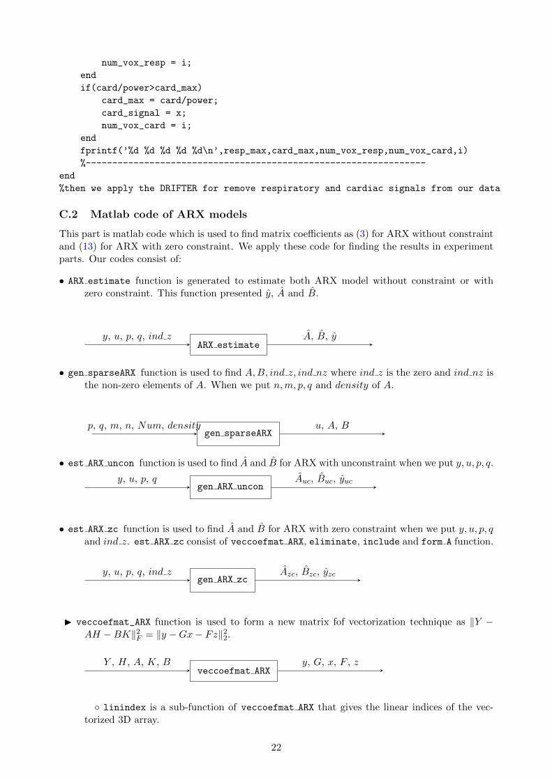
C.2 Matlab code of ARX models

This part is matlab code which is used to find matrix coefficients as (3) for ARX without constraintand (13) for ARX with zero constraint. We apply these code for finding the results in experimentparts. Our codes consist of:

• ARX estimate function is generated to estimate both ARX model without constraint or withzero constraint. This function presented y, A and B.

ARX estimatey, u, p, q, ind z A, B, y

• gen sparseARX function is used to find A,B, ind z, ind nz where ind z is the zero and ind nz isthe non-zero elements of A. When we put n,m, p, q and density of A.

gen sparseARXp, q, m, n, Num, density u, A, B

• est ARX uncon function is used to find A and B for ARX with unconstraint when we put y, u, p, q.

gen ARX uncony, u, p, q Auc, Buc, yuc

• est ARX zc function is used to find A and B for ARX with zero constraint when we put y, u, p, qand ind z. est ARX zc consist of veccoefmat ARX, eliminate, include and form A function.

gen ARX zcy, u, p, q, ind z Azc, Bzc, yzc

I veccoefmat_ARX function is used to form a new matrix fof vectorization technique as ‖Y −AH −BK‖2F = ‖y −Gx− Fz‖22.

veccoefmat ARXY , H, A, K, B y, G, x, F , z

◦ linindex is a sub-function of veccoefmat ARX that gives the linear indices of the vec-torized 3D array.

22

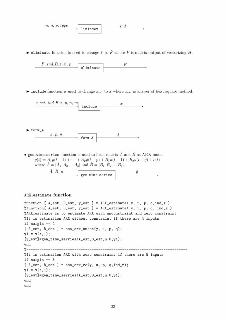
linindexm, n, p, type ind

I eliminate function is used to change F to F where F is matrix output of vectorizing H.

eliminateF , ind B z, n, p F

I include function is used to change xest to x where xest is answer of least square method.

includex est, ind B z, p, n, m x

I form_A

form Ax, p, n A

• gen time series function is used to form matrix A and B as ARX modely(t) = A1y(t− 1) + · · ·+Apy(t− p) +B1u(t− 1) +Bqu(t− q) + e(t)where A = [A1 A2 . . . Ap] and B = [B1 B2 . . . Bq].

gen time seriesA, B, u y

ARX estimate function

function [ A_est, B_est, y_est ] = ARX_estimate( y, u, p, q,ind_z )

%function[ A_est, B_est, y_est ] = ARX_estimate( y, u, p, q, ind_z )

%ARX_estimate is to estimate ARX with unconstraint and zero constraint

%It is estimation ARX without constraint if there are 4 inputs

if nargin == 4

[ A_est, B_est ] = est_arx_uncon(y, u, p, q);

y1 = y(:,1);

[y_est]=gen_time_serries(A_est,B_est,u,0,y1);

end

%--------------------------------------------------------------------------

%It is estimation ARX with zero constraint if there are 5 inputs

if nargin == 5

[ A_est, B_est ] = est_arx_zc(y, u, p, q,ind_z);

y1 = y(:,1);

[y_est]=gen_time_serries(A_est,B_est,u,0,y1);

end

end

23

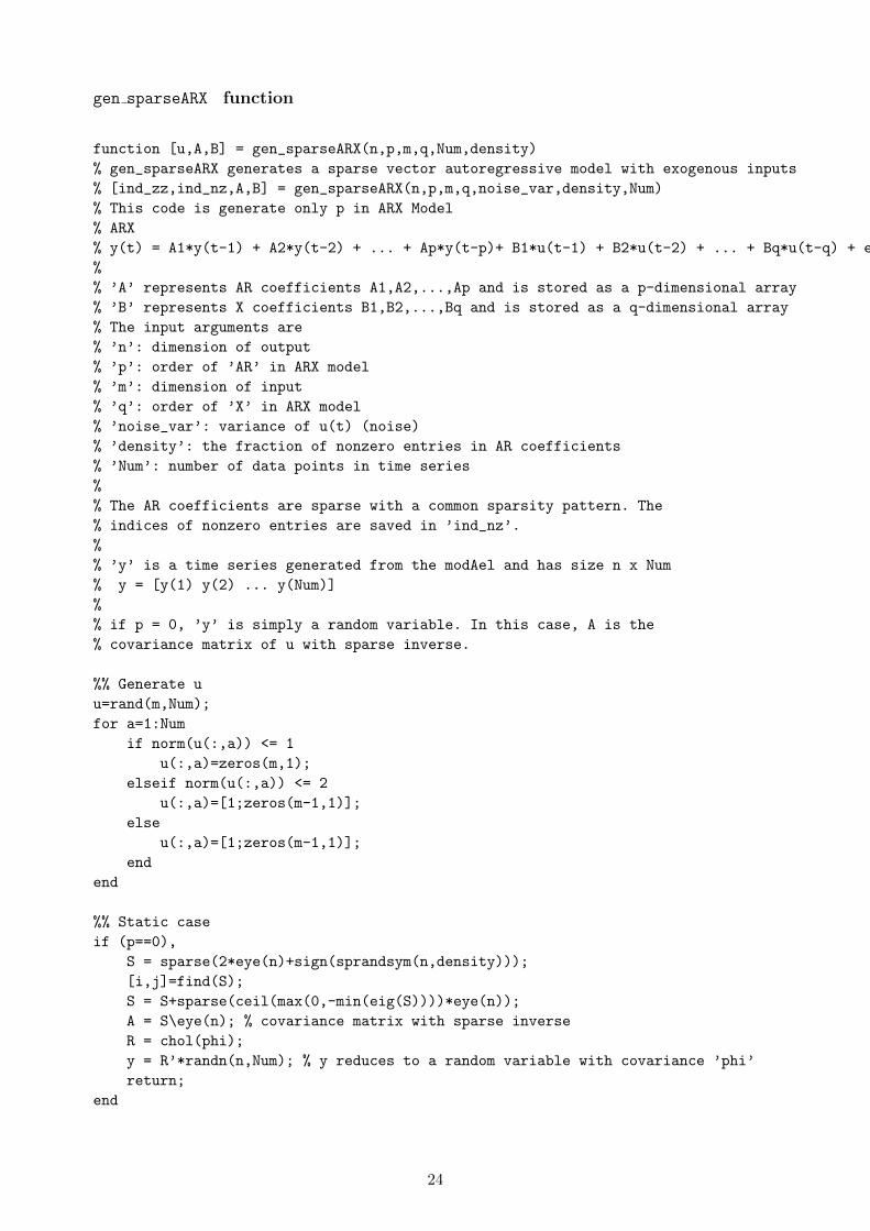
gen sparseARX function

function [u,A,B] = gen_sparseARX(n,p,m,q,Num,density)

% gen_sparseARX generates a sparse vector autoregressive model with exogenous inputs

% [ind_zz,ind_nz,A,B] = gen_sparseARX(n,p,m,q,noise_var,density,Num)

% This code is generate only p in ARX Model

% ARX

% y(t) = A1*y(t-1) + A2*y(t-2) + ... + Ap*y(t-p)+ B1*u(t-1) + B2*u(t-2) + ... + Bq*u(t-q) + e(t)

%

% ’A’ represents AR coefficients A1,A2,...,Ap and is stored as a p-dimensional array

% ’B’ represents X coefficients B1,B2,...,Bq and is stored as a q-dimensional array

% The input arguments are

% ’n’: dimension of output

% ’p’: order of ’AR’ in ARX model

% ’m’: dimension of input

% ’q’: order of ’X’ in ARX model

% ’noise_var’: variance of u(t) (noise)

% ’density’: the fraction of nonzero entries in AR coefficients

% ’Num’: number of data points in time series

%

% The AR coefficients are sparse with a common sparsity pattern. The

% indices of nonzero entries are saved in ’ind_nz’.

%

% ’y’ is a time series generated from the modAel and has size n x Num

% y = [y(1) y(2) ... y(Num)]

%

% if p = 0, ’y’ is simply a random variable. In this case, A is the

% covariance matrix of u with sparse inverse.

%% Generate u

u=rand(m,Num);

for a=1:Num

if norm(u(:,a)) <= 1

u(:,a)=zeros(m,1);

elseif norm(u(:,a)) <= 2

u(:,a)=[1;zeros(m-1,1)];

else

u(:,a)=[1;zeros(m-1,1)];

end

end

%% Static case

if (p==0),

S = sparse(2*eye(n)+sign(sprandsym(n,density)));

[i,j]=find(S);

S = S+sparse(ceil(max(0,-min(eig(S))))*eye(n));

A = S\eye(n); % covariance matrix with sparse inverse

R = chol(phi);

y = R’*randn(n,Num); % y reduces to a random variable with covariance ’phi’

return;

end

24

%% Randomize AR coefficients

MAX_EIG = 1;

diag_ind = find(eye(n));

k = length(diag_ind);

diag_ind3D = kron(n^2*(0:p-1)’,ones(k,1))+kron(ones(p,1),diag_ind);

A = zeros(n,n,p);

S = sprand(n,n,density)+eye(n);

ii = 0;

while MAX_EIG,

ii = ii+1;

for k=1:p,

A(:,:,k) = 0.1*sprandn(S);

end

%%%%%%%%%%%%%%%%%%%%%%%%%%%%%%%%%%%%%%%%%%%%%%%%

poles = -0.7+2*0.7*rand(n,p); % make the poles inside the unit circle

characeq = zeros(n,p+1);

for jj=1:n,

characeq(jj,:) = poly(poles(jj,:)); % each row is [1 -a1 -a2 ... -ap]

end

aux = -characeq(:,2:end);

A(diag_ind3D) = aux(:); % replace the diagonal entries with stable polynomial

%%%%%%%%%%%%%%%%%%%%%%%%%%%%%%%%%%%%%%%%%%%%%%%%

AA =[];

for k=1:p,

AA = [AA A(:,:,k)];

end

AA = sparse([AA ; [eye(n*(p-1)) zeros(n*(p-1),n)]]);

if max(abs(eigs(AA))) < 1

MAX_EIG = 0;

end

end

abs(eigs(AA))

ii

B=rand(n,m,q);

est arx uncon function

function [ A, B, y_est ] = est_arx_uncon(y, u, p, q)

% function [ A, B, y_est ] = est_arx_uncon(y, u, p, q)

% This function is generate

%y is output data with y=[y(1) y(2) ... y(N)]

%-------------------------------------------------------------------------%

[n,N]=size(y);

[row_u,col_u]=size(u);

%check error input

%Compute Y of measured output

Y = y(:,p+1:N);

%Compute matrix of causal sequence of output H_y

25

H_y=[];

for i= p:-1:1

H_y=[H_y ;y(:,i:end-p-1+i)];

end

%Compute matrix of causal sequence of input H_u

H_u=[];

for i= p:-1:p-q+1

H_u=[H_u;u(:,i:end-p-1+i)];

end

%Compute matrix H

H = [H_y; H_u];

%Estimate coefficient C

C = Y*pinv(H);

%Separate coefficient of input and coefficient of ouput

A0 = C(:,1:n*p);

B0 = C(:,n*p+1:end);

for i=1:p

A(:,:,i)=A0(:,1+n*(i-1):n*i);

end

for i=1:q

B(:,:,i)=B0(:,1+row_u*(i-1):row_u*i);

end

%Reshape matrix A into 2D

row_A2D = size(A,1);

col_A2D = size(A,2)*size(A,3);

A2D = reshape(A,[row_A2D, col_A2D]);

%Reshape matrix B into 2D

row_B2D = size(B,1);

col_B2D = size(B,2)*size(B,3);

B2D = reshape(B,[row_B2D, col_B2D]);

%estimated output

y_est = [A2D, B2D]*H;

end

est arx zc function

function [ A, B, y_est ] = est_arx_zc(y, u, p, q,ind_z)

% function [ A, B, y_est ] = est_arx_zc(y, u, p, q,ind_nz)

% This function estimate parameter in ARX model by using least square and

% zero constain

%

% input

% ’y’ is array of input

% ’u’ is array of input

% ’p’ is number of lag of in estimate AR factor in ARX

% ’q’ is number of lag of in estimate X factor in ARX

% ’ind_z’ are index of A is zero in AR factor

% output

% ’A’ are matrices of AR factor in ARX model

% ’B’ are matrices of X factor in ARX model

% ’y_est’ are estimated output from zero constraint

%%

26

[row_y,col_y]=size(y);


%% gen Y H K

Y=y(:,p+1:end);

H=[];

for i= p:-1:1

H=[H ;y(:,i:end-p+i-1)];

end

K=[];

for i= p:-1:p-q+1

K=[K;u(:,i:end-p+i-1)];

end

A=rand(row_y,row_y*p);

B=rand(row_y,row_u*q);

%% vectorization and solve least square

[y_vec,G,x,F,z] = veccoefmat_ARX(Y,H,A,K,B,row_u);

[row_z,col_z]=size(z);

[G_bar]=eliminate(G,ind_z,row_y,p);

xz_ls=[G_bar F]\y_vec;

[row_xz,col_xz]=size(xz_ls);

x_ls=xz_ls(1:row_xz-row_z,:);

z_ls=xz_ls(row_xz-row_z+1:end,:);

x=include(x_ls,ind_z,p,row_y,row_y);

%% create A,B form x,z and check A,B%%%%%%%%%%%%%%%%%%%%

A=form_A(x,p,row_y);

B=form_A(z_ls,q,row_y);

%% create estmated y%%%%%%%%%%%%%%%%%%%%

%Reshape matrix A into 2D

row_A2D = size(A,1);

col_A2D = size(A,2)*size(A,3);

A2D = reshape(A,[row_A2D, col_A2D]);

%Reshape matrix B into 2D

row_B2D = size(B,1);

col_B2D = size(B,2)*size(B,3);

B2D = reshape(B,[row_B2D, col_B2D]);

%estimated output

y_est = [A2D, B2D]*[H; K];

end

include function

function[x]=include(x_est,ind_B_z,p,n,m)

% this code is change x_est to x

% x_est is answer of least square method

% x is x_est that is included zeros elements

% x in R^nmp

% ind_B_nz is index of B that B(ind_B_nz) is not zero

% n is number of length of output y

% q is number of lag in matrix

x=[];

[I,J]=ind2sub([n m],ind_B_z);

27

[row_I,col_I]=size(I);

%% source I,J depend on J %%%%%%%%%%%%%%%%%%%%%%%%%%

for i=1:row_I

for j=1:i-1

fn_i=m*(I(i)-1)+J(i);

fn_j=m*(I(j)-1)+J(j);

if fn_i < fn_j

a=I(i);

b=J(i);

for k = i-1:-1:j

I(k+1)=I(k);

J(k+1)=J(k);

end

I(j)=a;

J(j)=b;

end

end

end

%% create x

k=1;

l=1;

for i=1:n*m

z_element=m*(I(k)-1)+J(k);

if i~=z_element

x=[x; x_est(p*(l-1)+1:p*l,:)];

l=l+1;

else

x=[x;zeros(p,1)];

k=k+1;

if k > row_I

x=[x; x_est(p*(l-1)+1:end,:)];

break

end

end

end

end

elimainate function

function[F_bar]=eliminate(F,ind_B_z,n,q)

% this code is change F to F_bar

% F is matrix output of vectorizing H

% F is R^nN*n*m*p

% F_bar is F that is elimated column relate x_i = 0

% ind_B_nz is index of B that B(ind_B_nz) is not zero

% n is number of length of output y

% q is number of lag in matrix

[row_F,col_F]=size(F);

m=floor(col_F/(n*q));

[I,J]=ind2sub([n m],ind_B_z);

[row_I,col_I]=size(I);

%% source I,J depend on J %%%%%%%%%%%%%%%%%%%%%%%%%%

28

for i=1:row_I

for j=1:i-1

fn_i=m*(I(i)-1)+J(i);

fn_j=m*(I(j)-1)+J(j);

if fn_i < fn_j

a=I(i);

b=J(i);

for k = i-1:-1:j

I(k+1)=I(k);

J(k+1)=J(k);

end

I(j)=a;

J(j)=b;

end

end

end

%%%%%%%%%%%%%%%%%%%%%%%%%%%%%%%%%%%%%%%%%%%%%%%%%%%%%%%%%%%%%%%%%%%%%

%% create F_bar %%%%%%%%%%%%%%%%%%%%%%%%%%%%%%%%%%%%%%%%%%%%%%%%

F_bar=[];

k=1;

for i=1:n*m

z_element=m*(I(k)-1)+J(k);

if i~=z_element

F_bar=[F_bar F(:,q*(i-1)+1:q*i)];

else

k=k+1;

if k > row_I

F_bar=[F_bar F(:,q*(i)+1:end)];

break

end

end

end

end

form A function

function[A]=form_A(x,p,n)

[row_x,col_x]=size(x);

nm=floor(row_x/p);

m=floor(nm/n);

for i=1:nm

lin_x(:,i)=x((i-1)*p+1:i*p,:);

end

for i=1:p

AA(:,i)=lin_x(i,:)’;

end

AAA=reshape(AA,m,n,p);

for i=1:p

A(:,:,i)=AAA(:,:,i)’;

end

end

29

gen time series function

function[y_time]=gen_time_series(A,B,u,noise_var)

% gen_time_series generates y in term of time series

%[y_time]=gen_time_series(A,B,u,noise_var)

% This code is generate only p in ARX Model

% ARX

% y(t) = A1*y(t-1) + A2*y(t-2) + ... + Ap*y(t-p)+ B1*u(t-1) + B2*u(t-2) + ... + Bq*u(t-q) + e(t)

% ’A’ represents A_est of AR coefficients A1,A2,...,Ap and is stored as a p-dimensional array

% ’B’ represents B_est of X coefficients B1,B2,...,Bq and is stored as a q-dimensional array

%

% The input arguments are

% ’A’: A_est that is estimated by est_ARX_uncon or est_ARX_zc function

% ’B’: B_est that is estimated by est_ARX_uncon or est_ARX_zc function

% ’u’: exogenous input which is generated form main.m

% ’noise_var’: variance of u(t) (noise)

%

%

[row_A,col_A,num_A]=size(A);

[row_B,col_B,num_B]=size(B);


sigma = noise_var;

y1 = rand(row_A, 1);

%% check error

if row_A ~= col_A

error(’uuhiuhiuhiuh’);

end

if row_A ~= row_B

error(’hoihijhojijojio’);

end

if col_B ~= row_u

error(’uhoiijojoijoijo’);

end

%gen time serries

y_time=[y1 zeros(row_A,col_u-1)];

for i=2:col_u

for j=1:num_A

if i - j > 1

y_time(:,i)=y_time(:,i)+A(:,:,j)*y_time(:,i-j);

end

end

for j=1:num_B

if i - j > 0

y_time(:,i)=y_time(:,i)+B(:,:,j)*u(:,j);

end

end

e = normrnd(0,sigma,[row_A 1]);

y_time(:,i)=y_time(:,i)+ e;

end

end

30

linindex function

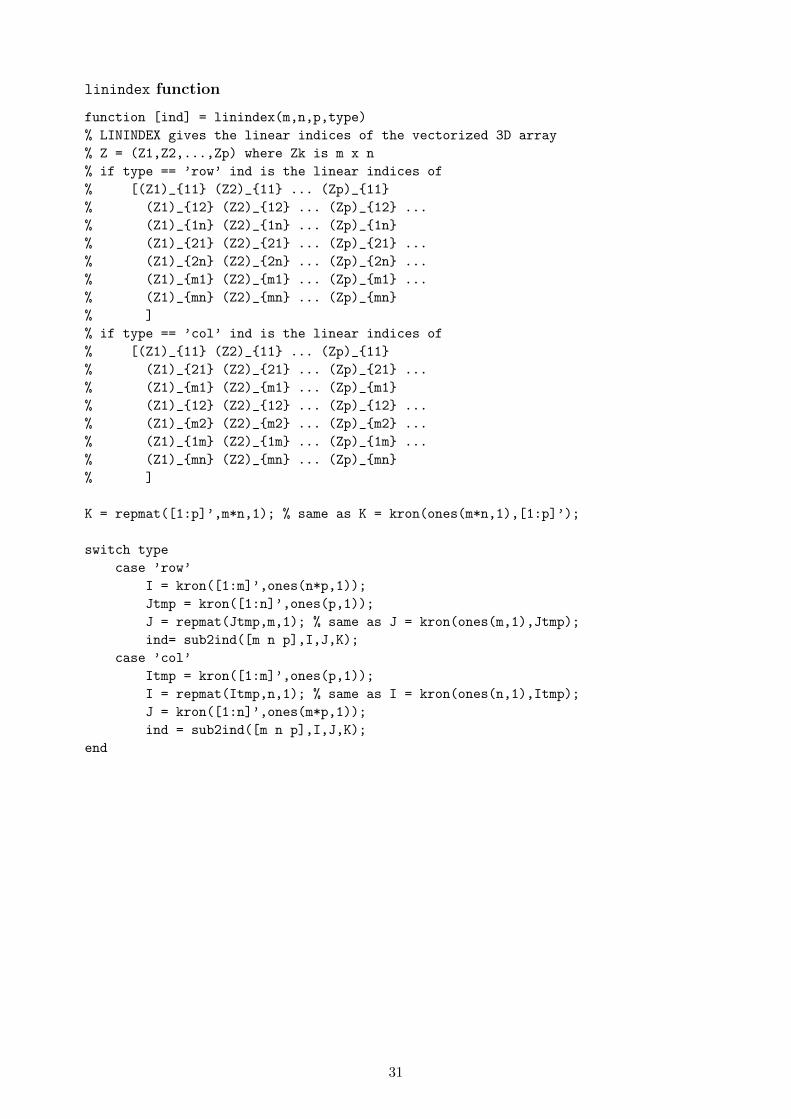
function [ind] = linindex(m,n,p,type)

% LININDEX gives the linear indices of the vectorized 3D array

% Z = (Z1,Z2,...,Zp) where Zk is m x n

% if type == ’row’ ind is the linear indices of

% [(Z1)_{11} (Z2)_{11} ... (Zp)_{11}

% (Z1)_{12} (Z2)_{12} ... (Zp)_{12} ...

% (Z1)_{1n} (Z2)_{1n} ... (Zp)_{1n}

% (Z1)_{21} (Z2)_{21} ... (Zp)_{21} ...

% (Z1)_{2n} (Z2)_{2n} ... (Zp)_{2n} ...

% (Z1)_{m1} (Z2)_{m1} ... (Zp)_{m1} ...

% (Z1)_{mn} (Z2)_{mn} ... (Zp)_{mn}

% ]

% if type == ’col’ ind is the linear indices of

% [(Z1)_{11} (Z2)_{11} ... (Zp)_{11}

% (Z1)_{21} (Z2)_{21} ... (Zp)_{21} ...

% (Z1)_{m1} (Z2)_{m1} ... (Zp)_{m1}

% (Z1)_{12} (Z2)_{12} ... (Zp)_{12} ...

% (Z1)_{m2} (Z2)_{m2} ... (Zp)_{m2} ...

% (Z1)_{1m} (Z2)_{1m} ... (Zp)_{1m} ...

% (Z1)_{mn} (Z2)_{mn} ... (Zp)_{mn}

% ]

K = repmat([1:p]’,m*n,1); % same as K = kron(ones(m*n,1),[1:p]’);

switch type

case ’row’

I = kron([1:m]’,ones(n*p,1));

Jtmp = kron([1:n]’,ones(p,1));

J = repmat(Jtmp,m,1); % same as J = kron(ones(m,1),Jtmp);

ind= sub2ind([m n p],I,J,K);

case ’col’

Itmp = kron([1:m]’,ones(p,1));

I = repmat(Itmp,n,1); % same as I = kron(ones(n,1),Itmp);

J = kron([1:n]’,ones(m*p,1));

ind = sub2ind([m n p],I,J,K);

end

31

Estimation of Autoregressive with Exogeneous Inputs...

Documents

Transcript of Estimation of Autoregressive with Exogeneous Inputs...