Time-Varying Autoregressive Model Based Signal Processing ...
152
Time-Varying Autoregressive Model Based Signal Processing with Applications to Interference Rejection in Spread Spectrum Communications by Peijun Shan Dissertation submitted to the faculty of the Virginia Polytechnic Institute and State University in partial fulfillment of the requirements for the degree of DOCTOR OF PHILOSOPHY in Electrical Engineering APPROVED: ____________________________ Dr. A. A. (Louis) Beex, Chairman ________________________ __________________ Dr. Hugh F. VanLandingham Dr. Brian D. Woerner ______________________ __________________ Dr. Theodore S. Rappaport Dr. Helen J. Crawford July 1999 Blacksburg, Virginia Keywords: Time-Varying Filtering, TVAR, Interference, Spread Spectrum, FM
Transcript of Time-Varying Autoregressive Model Based Signal Processing ...
Time-Varying Autoregressive Model Based Signal
Processing with Applications to Interference
Rejection in Spread Spectrum Communications
by
Peijun Shan
Dissertation submitted to the faculty of theVirginia Polytechnic Institute and State University
in partial fulfillment of the requirements for the degree of
DOCTOR OF PHILOSOPHYin
Electrical Engineering
APPROVED:
____________________________Dr. A. A. (Louis) Beex, Chairman
________________________ __________________Dr. Hugh F. VanLandingham Dr. Brian D. Woerner
______________________ __________________Dr. Theodore S. Rappaport Dr. Helen J. Crawford
July 1999Blacksburg, Virginia
Keywords: Time-Varying Filtering, TVAR, Interference, Spread Spectrum, FM

i
Time-Varying Autoregressive Model Based SignalProcessing with Applications to Interference Rejection in
Spread Spectrum Communications
by
Peijun ShanA. A. (Louis) Beex, Chairman
Electrical Engineering
(ABSTRACT)
The objective of this research is to develop time-varying signal processingmethods for rapidly varying non-stationary signals based on time-varying autoregressive(TVAR) modeling, and to apply such methods to frequency-modulated (FM) interferencerejection in direct-sequence spread spectrum (DSSS) communications. For fast varyingnon-stationary signal processing, such as the task to reject an FM interference that couldchirp over the entire DSSS bandwidth in a symbol interval, an explicit description of thevariation is necessary to form a time-varying filter. This is realized using the TVARmodel, which is an autoregressive model whose coefficients are time-varying with thevariation modeled as a linear combination of a set of known functions of time. In DSSScommunications, when the strength of an interference - which could be a hostile jammeror overlaid communication signal - possibly exceeds the inherent spread spectrumprocessing gain, interference rejection is necessary to secure a usable bit-error-rate.
The contributions of this research include: a) revealed the advantageousperformance of TVAR model based instantaneous frequency estimation (TVAR-IF),which is expected to change the prevailing opinion that regards TVAR-IF as a poorestimator; b) proposed a time-varying Prony method to improve TVAR-IF at low SNR;c) proposed to use TVAR-IF for time-varying FIR notch filter based FM jammersuppression in DSSS communications; d) developed TVAR model based time-varyingoptimum filters, including the TVAR based Kalman filter (TVAR-KF) and the TVARbased Wiener filter (TVAR-WF); e) developed a TVAR-WF based formulation of FMinterference soft-cancellation in DSSS communications; and f) proposed a TVAR basedlinear prediction error (TVAR-LPE) filter for soft-cancellation of FM interference inDSSS communications.
For the interference rejection problem, our TVAR-IF controlled notch filter yieldshigh processing gain close to that using the known IF and much higher than that using theWVD based IF estimate. Furthermore, unlike the IF based notch filter approaches, theproposed soft-cancellation methods utilize the full spectral information captured by theTVAR model. Our soft-cancellation approaches, including TVAR-WF and TVAR-LPE,maintain at least the DSSS system performance expected when no filtering is used, evenunder estimated conditions. The latter is in contrast to the notch filter based approaches,which may cause deterioration of overall system performance at low jammer-to-signalratios.

ii
Acknowledgments
Foremost, I wish to express my deepest gratitude to my advisor, Dr. A. A. (Louis)
Beex, for being an excellent professor guiding me through the journey. Without his
advice, insight, encouragement, patience and support, this work would be impossible. I
am grateful to his generous sacrifice in time and financial support.
I extend my sincere thanks to Dr. Brian D. Woerner, Dr. Hugh F.
VanLandingham, Dr. Theodore S. Rappaport and Dr. Helen J. Crawford for spending
their time serving on my advisory committee. It is Dr. Woerner who introduced me to the
field of spread spectrum communications and DSSS receivers.
My gratitude also goes to Dr. Karl H. Pribram and Dr. Joe S. King, both at the
Center for Brain Research and Information Sciences at Radford University, for their
years of support.
My special appreciation goes to my wife, my parents, my parents-in-law, my
brother, my brother-in-law, and my daughters. It is their sacrifice, encouragement,
support, understanding and compassion, one way or another, that makes this work
possible and meaningful.

iii
“The Times, They Are A-Changin’.”
by Bob Dylan (1941- )
“All is flux, nothing is stationary.”
“Change alone is unchanging.”
by Heraclitus (c. 535–c. 475 B.C.)
Contents
1. Introduction and Literature Review 1
1.1 Time-Varying Filtering 11.2 Time-Varying Wiener Filtering 31.3 Instantaneous Frequency Estimation 51.4 Time-Varying Interference Suppression for Direct Sequence
Spread Spectrum (DSSS) Communications. 71.5 Introduction to the Time-Varying Autoregressive (TVAR) Model 101.6 Research Motivations and Objectives 131.7 Research Outline 14
1.7.1 Instantaneous Frequency (IF) Estimation Based on TVAR Modeling 151.7.2 FM Interference Suppression for Direct Sequence Spread Spectrum
Communications Using TVAR based IF Estimation 151.7.3 Time-Varying Optimum Filtering Based on TVAR Modeling 161.7.4 FM Interference Cancellation Based on TVAR Wiener Filtering 161.7.5 Time-Varying Whitening Filter Based on the TVAR Model for FM
Interference Cancellation in DSSS Communications 17
2. Instantaneous Frequency Estimation Based on TVAR Modeling 18
2.1 Introduction 182.2 TVAR Based IF Estimation: Method and Examples 20
2.2.1 Method 202.2.2 Example 1: A Chirp Signal 212.2.3 Example 2: A Frequency-Hopping Signal 27
2.3 Performance of TVAR Based IF Estimation 282.3.1 Experiment Setup and Implementation 312.3.2 Linear FM Signal Scenarios 322.3.3 Non-Linear FM Signal Scenarios 36
2.4 Summary 40

iv
3. A Time-Varying Prony Method for IF Estimation at Low SNR 41
3.1 Introduction 413.2 A Time-Varying Prony Method: Method and Example 43
3.2.1 Method 433.2.2 Example 45
3.3 Performance of the Time-Varying Prony Method 483.3.1 Case 1: Non-monotonic Nonlinear FM 483.3.2 Case 2: Monotonic Nonlinear FM 513.3.3 Case 3: a Linear FM 52
3.4 Summary 53
4. Notch Filter Based Interference Suppression UsingTVAR Based IF Estimation 54
4.1 Introduction 554.2 Notch Filter Based FM Interference Suppression Using TVAR Based IF
Estimation 564.3 System Performance Improvement Due to Interference Rejection
Using TVAR Based IF Estimation 574.3.1 Experiment Setup and Implementation 584.3.2 Linear FM Interference 604.3.3 Non-Linear FM Interference 624.3.4 Multiple-FM Interference 66
4.4 Summary and Discussion 72
5. Time-Varying Optimum Filtering 73
5.1 Introduction 735.2 Wiener Filtering 74
5.2.1 General Time-Varying Wiener Filter 745.2.2 FIR Wiener Filter 765.2.3 IIR Wiener Filter 77
5.3 Kalman Filtering 795.4 Summary and Discussion 82
6. Time-Varying Optimum Filtering Based on TVAR Modeling 83
6.1 Introduction 836.2 TVAR Kalman Filter 85
6.2.1 Method 856.2.2 Example 86
6.3 TVAR Wiener Filter 896.3.1 Method 896.3.2 Example 93
6.4 Simulation Results for TVAR Based Optimum Filters 976.5 Summary 101

v
7. Soft-Cancellation of FM Interference Based onOptimal Filtering 102
7.1 Introduction 1027.2 A General Description of Interference Suppression Based on
TVAR Modeling 1047.3 FM Interference Suppression Based on TVAR-WF: Method and Example 105
7.3.1 Method 1057.3.2 Example 109
7.4 Simulations of Interference Suppression Based on TVAR-WF 1107.4.1 Case 1: Fixed-Frequency and Known Parameters 1127.4.2 Case 2: Nonlinear FM Jammer Using Estimated Parameters 113
7.5 Summary and Discussion 116
8. TVAR BASED Time-Varying Whitening Filter for Soft-Cancellation of FM Interference in DSSS 117
8.1 Introduction 1178.2 FM Interference Suppression Based on TVAR Whitening
Filter: Method and Example 1198.2.1 Method 1198.2.2 Example 121
8.3 Simulations on TVAR-LPE and an Extensive Comparison 1238.4 Summary and Discussion 129
9. Summary and Suggestions for Future Work 130
9.1 Summary 1309.2 Suggestions for Future Work 132
Appendix 134A Wigner-Ville Distribution (WVD) and WVD Peak Based IF Estimation 134
A-1 Wigner-Ville Distribution (WVD) 134A-2 WVD Based IF Estimation (WVD-IF) 135A-3 Example of WVD and WVD-IF 135
B Evolutionary Spectrum Theory and its Relation to this Work 137B-1 Review of Priestley’s Evolutionary Spectrum Theory 137B-2 Relation of Priestley’s Evolutionary Spectrum Theory to this Work 138
Bibliography 141
Vita 146

Chapter 1 Introduction and Literature Review
1
Chapter 1
INTRODUCTION AND LITERATURE REVIEW
This research explores and develops parametric model based time-varying signal
processing methods, including time-varying Wiener filtering (TVWF) and instantaneous
frequency (IF) estimation, as well as their applications to interference suppression for
spread spectrum (SS) communications. In this chapter we review the related works in the
literature.
1.1 Time-Varying Filtering
Before addressing the time-varying Wiener filtering problem, we first review the
studies on time-varying filtering. Time-frequency analysis has been one of the most
active research areas in the signal processing community over the past two decades.
Besides a large amount of work on time-frequency analysis, there has also been
substantial research effort on time-frequency based signal processing, i.e. processing
signals in the time-frequency plane, usually using the information obtained from time-
frequency analysis. In time-frequency filtering problems, both the desired signal and the
contaminating noise may be nonstationary and, in general, can not be separated by either

Chapter 1 Introduction and Literature Review
2
temporal windowing or conventional time-invariant frequency-selective filtering, and
therefore filtering in the joint time-frequency domain is necessitated.
The earlier methods of time-frequency filtering were based on signal synthesis [1-
3]. These methods operated in a procedure consisting of three steps: 1) “transform” the
original observed signal to some form of time-frequency representation (TFR) [32], linear
or nonlinear, such as the short-time Fourier transform (STFT), Wigner-Ville Distribution
(WVD), or some other Cohen class of TFR [4]; 2) mask the TFR of the observed signal
to retain the desired signal component(s) and excise the unwanted component(s); and 3)
synthesize the filtered signal from the masked TFR. In 1986, Boudreaux-Bartels and
Parks [1] first proposed the time-frequency filter based on WVD synthesis. Since the
masked TFR may not be a valid TFR, approximation and optimization were often needed
in the final step of signal synthesis. This type of filtering operation was highly non-linear
and usually very demanding computationally. In addition, the performance of the WVD
synthesis based filtering procedure was shown to be potentially poor [5, 2]. Linear TFRs,
such as the STFT [6-8], the Gabor Transform [9], and the Wavelet Transform [10], were
also used for time-frequency filtering in a similar way. A major drawback of these linear
TFR based filters was the limitation of the time-frequency resolution inherited with these
TFRs.
In the early 1990’s, the studies on time-frequency filtering shifted from signal
synthesis to time-frequency projection filters [11-15]. A time-frequency projection filter
is an orthogonal projection operator of a linear signal space. The filter design was
accomplished by constructing an optimal linear signal space corresponding to the time-
frequency pass-region [12, 13]. A more general linear time-varying filter design method

Chapter 1 Introduction and Literature Review
3
based on Weyl Correspondence (WC) was investigated [14, 15]. It was illustrated that the
WC based filter performed better than the signal synthesis methods [15].
In the mid 1990’s, time-frequency strip filters [16-18], including fractional
Fourier domain filters [18], were proposed for the special cases where the pass-regions in
the time-frequency plane are in strip shapes. A strip filter first rotates the signal in the
time-frequency plane to make the strip-shaped pass-region perpendicular to the time axis,
then windows the rotated signal such that the desired signal is retained and the unwanted
components are suppressed, and finally reverses the rotation to obtain the filtered signal.
Conventional time-domain windowing and linear time-invariant (LTV) filtering can be
viewed as special cases of strip filtering with rotation angles of 0 and 90 degrees
respectively.
1.2 Time-Varying Wiener Filtering
The time-varying filtering methods mentioned above are generally pass-stop type
of operations in the time-frequency plane, under the assumption that the desired signal
and the undesired component(s) have disjoint time-frequency supports. In stationary
cases, this corresponds to the classical pass-stop filtering, such as low/high/band pass
filters and notch filters. Of major interest in this research are the more general cases
where the signal and noise have overlapping time-frequency supports and both may have
broad instantaneous bandwidths. We aim at achieving optimal or nearly optimal
estimation of the desired signal based on the least mean square error criterion and refer to
this problem as one of time-varying Wiener filtering (TVWF). This is the signal

Chapter 1 Introduction and Literature Review
4
estimation problem corresponding to the stationary case where optimal filters, referred to
as Wiener Filters (WF) [19], are designed based on the mean-square error criterion.
To solve for the impulse response of the optimal filter from the autocorrelation
functions of the signal and noise requires solving an integral equation known as the
Wiener-Hopf equation [19], which, for stationary processes, reduces to a deconvolution
problem. For wide-sense stationary processes, the optimal filter can be easily formulated
in the frequency domain [19, 37]. For nonstationary cases, this problem, referred to as
nonstationary Wiener filtering or time-varying Wiener filtering (TVWF), has been
addressed by a few researchers from different points of view [20-23].
The earliest effort in TVWF was due to Abdrabbo and Priestley [20] in 1969,
although it was not much noticed by the signal processing community then. The filtering
was based on Priestley’s evolutionary spectrum theory [24]. In 1995, Kirchauer,
Hlawatsch and Kozek [21] proposed a time-frequency formulation of nonstationary
Wiener filters. This work extended the spectral representation of stationary Wiener filters
to the nonstationary case based on the Wigner-Ville Distribution (WVD) and the Weyl
Symbol (WS) of linear operators. At the same time, Beex and Xie [22] proposed a time-
varying Wiener filtering method based on their Multi-resolution Parametric Spectral
Estimator (MPSE) [25, 26]. This method used sliding data windows and assumed local
stationarity inside each sliding temporal window. It exhibited significant signal to noise
ratio (SNR) gain for moderately slowly time-varying signals. More recently, Khan and
Chaparro [23] further studied non-stationary Wiener filtering based on evolutionary
spectral theory. They considered two cases of uncorrelation between the signal and the
noise: disjoint supports of the generating kernels of the signal and noise, and orthogonal

Chapter 1 Introduction and Literature Review
5
innovation processes of the signal and noise. For the latter case, their solution coincided
with that of Abdrabbo and Priestley [20].
In the present study, a new method for TVWF design is proposed [27] and will be
investigated further. It is based on time-varying AR (TVAR) modeling [28, 29], i.e.
modeling the signal and noise as auto-regressive processes with time-varying coefficients
which are further modeled as combinations of a set of known functions of time.
1.3 Instantaneous Frequency Estimation
Time-frequency analysis is an extension of stationary spectral analysis. Time-
varying filtering, or alternatively, time-frequency filtering, is an extension of the time-
invariant filtering problem. In the same way, instantaneous frequency (IF) estimation can
be viewed as an extension of stationary sinusoidal frequency estimation [30]. While these
stationary problems have been studied extensively, there is still much unsolved for their
nonstationary extensions. An extensive review on instantaneous frequency estimation
techniques was contributed by Boashash [31] in 1992. According to this review and the
references therein, the “primitive” methods such as phase difference estimators and zero-
crossing IF estimators are conceptually and computationally simple, but they perform
poorly for noisy signals. The Phase Locked Loops (PLL), which can be easily built and
are widely used in communications systems, are a form of adaptive IF estimation. The
PLL is relatively noise resistant, but is unable to track a wide ranging or rapidly varying
frequency. Other adaptive IF estimation algorithms were developed, such as those based
on Kalman filtering theory and those combining stationary auto-regressive (AR)
modeling and adaptive filtering algorithms. The Kalman filtering based method can be

Chapter 1 Introduction and Literature Review
6
viewed as an extension of the PLL. All the PLL, Kalman filtering, and adaptive filtering
based IF estimation methods are essentially IF tracking processes and therefore unable to
respond to very rapidly varying frequencies.
An important class of IF estimation methods is based on TFR or time-frequency
distributions (TFD). Any appropriate TFD, such as the spectrogram and WVD, can be
applied to IF estimation. The IF is estimated through either peak detection or first-
moment estimation of TFDs. For lower SNR, Boashash suggested an iterative procedure
of combining time-frequency filtering and moment estimation to improve IF estimation
[3]. Among these, WVD peak based IF estimation was reported to be optimal for linear
frequency modulated (FM) signals with high to moderate SNR [33] and hence was
recommended [31]. The present research [34] revealed that the optimality of the WVD
based method requires the following conditions simultaneously: 1) a linear FM signal, 2)
the time instances of the estimated IF are far from the data ends, 3) generous zero-
padding or frequency interpolation, and 4) high SNR. Violation of any one of these
conditions can lead to a performance ceiling for the WVD based method [34].
The TFD based IF estimators are non-parametric in the sense that there is no
parametric modeling applied to the observation data, although by modeling the IF laws
one can improve the TFD based estimators [35]. An extensively studied class of
parametric IF estimation methods is based on polynomial phase modeling, i.e., modeling
the signal as a complex exponential function with phase in the form of a finite order
polynomial function of time. The polynomial coefficients for the phase can be estimated
by solving a non-linear regression problem somehow or by a multi-dimensional search
which leads to ML estimates [31].

Chapter 1 Introduction and Literature Review
7
The last IF estimation method to be introduced here is the IF estimation based on
time-varying AR (TVAR) modeling, proposed by Sharman and Friedlander in 1984 [36].
Since being proposed, this method has been considered a poor estimator [31, 36] and, as a
result, there has not been much further study of this method reported in the literature. As
part of this research, we again study this approach. Our preliminary work has shown that
the TVAR based method, though not optimal in any case, is robust and performs
satisfactorily in various situations [34].
1.4 Time-Varying Interference Suppression for Direct Sequence Spread
Spectrum (DSSS) Communications
A spread spectrum communication system uses a transmission bandwidth that is
purposely made wider than the necessary information bandwidth of the signal. The
spectrum spreading is typically accomplished with techniques such as direct sequence
(DS), frequency hopping (FH), or a hybrid of DS and FH. The advantages of the spread
spectrum techniques include low probability of signal interception, protection against
interference and hostile jamming, resistance to multipath fading, and efficiency of
frequency reuse. Based on the direct sequence spread spectrum (DSSS) technique the
prevailing code-division multiple access (CDMA) systems were proposed and built. In
the present study, we focus on the nonstationary interference suppression problem for
DSSS communications.
The benefit of the immunity to noise and interference of a DSSS system is
referred to as “processing gain.” However, excessive noise and/or interference beyond
the protection of the processing gain still jeopardize the system. While an adequate signal

Chapter 1 Introduction and Literature Review
8
to noise ratio (SNR) can be assured by proper link budget design, it is impractical to
predict or avoid excessive interference from uncooperative sources. Interference in a
DSSS system can be classified into the following categories: 1) multiple access
interference (MAI) in CDMA from other users’ signals, 2) hostile jamming, and 3) co-
channel interference from other sources, including other communications systems. MAI
is usually mitigated through power control and multiuser detection techniques, which
have been actively studied in recent years [42, 43 and the references therein]. This
research focuses on suppression techniques for time-varying interference from jammer or
overlaid communication systems, such as the FM signal from an AMPS system overlaid
with a CDMA system.
In a direct sequence CDMA system, MAI has the same spectral characteristic as
the signal of the desired user. Therefore, in general, MAI can not be mitigated through
temporal filtering. Instead, the cancellation of MAI exploits either 1) the cross-correlation
among the spreading codes of all users in a cell, which results in decorrelating multiuser
receivers, 2) temporary decisions of all the users, which results in multi-stage interference
cancellation multiuser receivers, or 3) spatial information from antenna arrays. In
contrast, non-MAI interference usually has spectral characteristics different from the
desired spread spectrum signal, and therefore temporal signal processing can help to
improve the system performance.
In 1986, Milstein and Iltis [44] reviewed the earlier studies on interference
rejection in spread spectrum communications, including least-squares estimation
techniques, Fourier frequency domain processing, and adaptive spatial filtering. In the
reviewed works it was assumed that the interference was stationary or slowly time-

Chapter 1 Introduction and Literature Review
9
varying and, therefore, traditional LTI filters were applied for the stationary cases and the
adaptive algorithms were effective in tracking the changes. Later, the discrete wavelet
transform (DWT) was applied to reject pulse jamming or interference with burst
characteristics [45], in a similar way as the Fourier transform domain method for tone
jamming or stationary narrow-band interference [46].
In recent years, time-frequency distributions are being applied to handle rapidly
varying nonstationary interference in DSSS communications [47-50]. Amin and his
colleagues [47, 48] studied interference excision using a time-varying notch filter with
the null placed at the instantaneous frequency (IF) of the interference, where the IF was
estimated from time-frequency distributions (TFD). The study suggested using the
length-5 symmetric zero-phase transversal filter with the second order zero placed at the
IF of the interference on the unit circle. The authors [49] also studied interference
cancellation using the time-frequency synthesis technique mentioned in Section 1.1 as a
method for time-varying filtering. With the assumption of constant modulus interference,
the interference is synthesized in two steps: first the interference is synthesized by
masking the time-frequency distribution of the received signal, and then the estimation is
improved by projecting the synthesized signal onto a circle representing the space of the
constant modulus jammer. The final jammer estimate was subtracted from the received
signal and, by doing so, system performance was improved significantly. Bultan and
Akansu [50] applied chirplet decomposition [51] to detect and excise the interference that
was localized in the time-frequency plane. This technique used the iterative algorithm of
matching pursuits [52] to extract the interference from the received signal. In all the
Chapter 1 Introduction and Literature Review
10
above time-frequency methods the interference was assumed to have narrow
instantaneous bandwidth, as typical for FM signals.
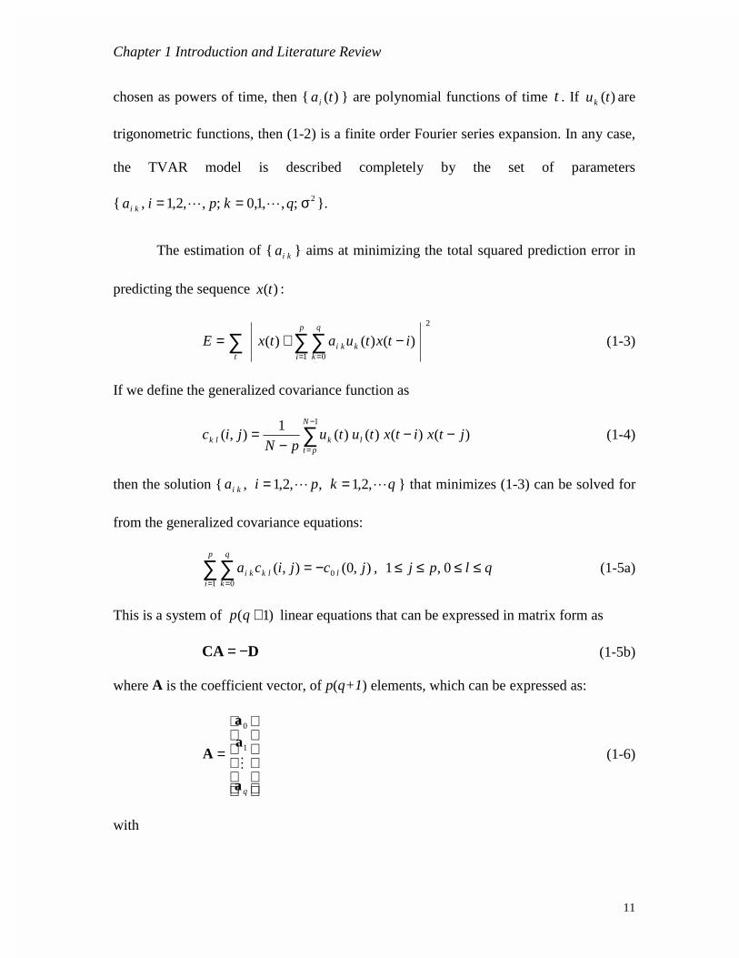
1.5 Introduction to the Time-Varying Autoregressive (TVAR) Model
In this section we review the time-varying autoregressive (TVAR) model, which
will be used throughout the following chapters. The idea of modeling a nonstationary
time series with time-dependent parameters was first proposed by Rao [41] in 1970 and
was studied by Liporace [61] soon after. It was not used for signal processing problems
until Hall, Oppenheim and Willsky [28] and Grenier [29] investigated modeling and
time-varying spectral estimation of speech signals with this type of model. Soon
thereafter, in 1984, Sharman and Friedlander [36] proposed the idea of using time-
varying AR (TVAR) modeling for instantaneous frequency estimation.
A discrete-time time-varying autoregressive (TVAR) process )(tx of order p is
expressed as
)()()()(1
teitxtatxp
ii +−−= ∑
=(1-1)
where )(te is a stationary white noise process with zero mean and variance 2eσ , and the
TVAR coefficients { )(tai , pi ,,2,1 �= } are modeled by linear combinations of a set of
basis time functions { )(tuk , qk ,,1,0 �= }:
)()(0
tuata k
q
kkii ∑
=
= (1-2)
where { qktuk ,,1,0),( �= } can be any appropriate set of basis functions. If { )(tuk } are
Chapter 1 Introduction and Literature Review
11
chosen as powers of time, then { )(tai } are polynomial functions of time t . If )(tuk are
trigonometric functions, then (1-2) is a finite order Fourier series expansion. In any case,
the TVAR model is described completely by the set of parameters
{ 2;,,1,0;,,2,1, σ== qkpia ki �� }.
The estimation of { kia } aims at minimizing the total squared prediction error in
predicting the sequence )(tx :
2
1 0
)()()( ∑∑∑= =
−+=p
ik
q
kki
t
itxtuatxE (1-3)
If we define the generalized covariance function as
)()()()(1
),(1
jtxitxtutupN
jic l
N
ptklk −−
−= ∑
−
=(1-4)
then the solution { qkpia ki �� ,2,1,,2,1, == } that minimizes (1-3) can be solved for
from the generalized covariance equations:
),0(),( 01 0
jcjica llk
p
i
q
kki −=∑∑
= =
, qlpj ≤≤≤≤ 0,1 (1-5a)
This is a system of )1( +qp linear equations that can be expressed in matrix form as
DCA −= (1-5b)
where A is the coefficient vector, of p(q+1) elements, which can be expressed as:
=
qa
a
a
A�
1
0
(1-6)
with

Chapter 1 Introduction and Literature Review
12
=
pk
k
k
k
a
a
a
�
2
1
a , qk ,,1,0 �= , (1-7)
and C is the extended covariance matrix of size p(q+1) by p(q+1):
=
qqqq
q
q
ccc
ccc
ccc
C
�
����
�
�
10
11110
00100
(1-8)
with
=
),()2,()1,(
),2()2,2()1,2(
),1()2,1()1,1(
ppcpcpc
pccc
pccc
klklkl
klklkl
klklkl
kl
�
����
�
�
c , qlqk ≤≤≤≤ 0,1 , (1-9)
and
=
qd
d
d
D�
1
0
(1-10)
with
=
),0(
)2,0(
)1,0(
0
0
0
pc
c
c
k
k
k
k�
d , qk �,1,0= . (1-11)
For the special case of 0=q , the above system of equations reduces to the Yule-
Walker Equations for the stationary AR model.

Chapter 1 Introduction and Literature Review
13
If we change the summation interval in (1-4) from [p, N −1] to [ ∞+∞− , ], or
equivalently [0, N−1+ p], by assuming that the data can be extended by zeros outside the
data record, the resulting equations (1-5) are the generalized correlation equations.
The matrices klc = lkc are )( pp× symmetric. Therefore, C is a )1()1( +×+ qq
block symmetric matrix with ( pp× ) symmetric blocks. C is not Toeplitz, and hence the
Levinson algorithm [30] can not be applied directly. For the correlation method, the
matrix C is symmetric and block-Toeplitz so that a modified version of the Levinson
algorithm can be used to solve (1-5) fast [29]. For the covariance method, the symmetry
structure can also be explored to solve (1-5) [29].
1.6 Research Motivations and Objectives
In this section, we define our research objectives and outline. Our general
motivation is to develop non-stationary signal processing methods based on time-varying
parametric modeling. This is different from the parametric non-stationary signal
processing methods based on temporal windowing, where stationary modeling is applied
inside each data window [26]. It is also different from another type of extensively studied
and applied time-varying signal processing − adaptive signal processing [38], where
training data is required so that it is not suitable for short data records and rapidly varying
processes. Our research is aimed at a better ability to handle rapidly varying signals and
short data records. We consider short data records due to the fact that in many
applications it is either desirable to deal with a smaller number of samples or only short
data records are available.

Chapter 1 Introduction and Literature Review
14
Parametric stationary signal processing has been studied extensively in the past
decades. Due to its attractive properties, such as high resolution, low computational
complexity and noise resistance, applications can be found in a variety of areas, such as
speech processing, radar/sonar, biomedical engineering and neural science. As a matter of
fact, in many practical situations, most signals are non-stationary in nature. It may be of
advantage to exploit non-stationary or as they are alternatively referred to, time-varying
signal processing methods. As seen in Sections 1.1 through 1.3, most of the existing time-
varying signal processing approaches are nonparametric. Our objective is to develop
signal processing methods which combine the advantages of being both time-varying and
parametric. Specifically, we focus on time-varying Wiener filtering and instantaneous
frequency estimation, as well as their potential applications in interference suppression
for spread spectrum communications.
We expect that the parametric time-varying signal processing methods under
development have many potential applications. The scenario of most interest to us in this
research is the time-varying interference suppression problem in communications. We
apply the TVAR based IF estimator to time-varying notch filtering for cancellation of
interference with narrow instantaneous bandwidth. We also formulate a nearly optimal
time-varying interference suppression filter based on the idea of the TVWF proposed in
this study.
1.7 Research Outline
The outline of the present research is presented below. The research work is
divided into five parts. In summary, in this research, we plan to develop a time-varying

Chapter 1 Introduction and Literature Review
15
signal processing method based on TVAR modeling, and to explore a TVAR based IF
estimation method. After validating the performance of these methods, they are applied to
improve the performance of DSSS communication systems by suppressing time-varying
interference.
1.7.1 Instantaneous Frequency (IF) Estimation Based on TVAR Modeling
First, we will examine the performance of TVAR based IF estimation, especially
for the case of short data records, and compare with WVD peak based IF estimation. The
TVAR method is expected to provide robust performance in moderate to high SNR and
under various conditions such as linear or non-linear IF laws, shorter or longer data
records, and close to or far from the ends of data blocks.
Then we will improve the performance of the TVAR based IF estimation method
for low SNR environments. A higher model order is used to let the extra poles capture a
portion of the noise components and the signal poles are distinguished from the noise
poles based on a “best subset” criterion, which is to be developed further for the time-
varying case. This idea was proven effective in the stationary case [53], and is expected
to be extendable to the time-varying case.
1.7.2 FM Interference Suppression for Direct Sequence Spread Spectrum
Communications Using TVAR based IF Estimation
After examining the performance advantages of the TVAR based IF estimation,
we apply it to notch filter based FM interference suppression in DSSS communications.
We will examine the system BER performance improvements due to the interference

Chapter 1 Introduction and Literature Review
16
cancellation using the TVAR based IF estimation, compare it with using the exact IF
(supposedly known) and the existing method that uses the Wigner-Ville distribution
(WVD) based IF estimates.
1.7.3 Time-Varying Optimum Filtering Based on TVAR Modeling
In the second part of the research, we develop TVAR model based optimum
filtering methods, including the TVAR based Kalman filter and TVAR based Wiener
filters. These formulations directly relate the filter parameters to the model parameters
and provide optimum or nearly-optimum time-varying filters. The modeling parameters
are identified from a block of observation data with the aid of a priori information. We
will examine the performance of the proposed TVAR based filters through simulations,
with both exact (supposedly known) TVAR parameters and estimated parameters. The
comparison will show that the non-causal TVAR based Wiener filter performs
significantly better than the TVAR based Kalman filter, which is the optimal causal filter.
It will also be revealed that the causal TVAR based Wiener filter performs almost the
same as the Kalman filter, and, therefore, is a nearly-optimum causal filter.
1.7.4 FM Interference Cancellation Based on TVAR Wiener Filtering
The TVAR based Wiener filter will be applied to perform time-varying
interference suppression filtering for DSSS communications. Unlike the notch filter
based cancellation method which uses only the frequency information to form a deep
notch, this method is aimed at minimum signal distortion and exploits the full spectral
information. We will examine the system BER performance improvements due to

Chapter 1 Introduction and Literature Review
17
application of the proposed filter and compare it with the notch filter method with exact
IF information used.
1.7.5 Time-Varying Whitening Filter Based on the TVAR Model for FM
Interference Cancellation in DSSS Communications
Finally, we will propose a simple, yet effective time-varying FIR filter for FM
interference suppression filtering in DSSS communications. It is aimed at the spectral
flatness of the filter output and is formed as the TVAR based linear prediction error filter.
We will examine the system BER performance improvements due to application of the
proposed filter and compare it with other methods.

Chapter 2 Instantaneous Frequency Estimation Based on TVAR Modeling
18
Chapter 2
INSTANTANEOUS FREQUENCY ESTIMATION
BASED ON TVAR MODELING
In this chapter, we introduce the TVAR based instantaneous frequency (IF)
estimation method, and examine its performance by comparing it with the WVD peak
based method for IF estimation through simulations. This work leads us to make a
conclusion about TVAR based IF estimation that is contrary to the prevailing conclusion
in the literature. The major content of this chapter was published earlier [34].
2.1 Introduction
For an observed signal consisting of single or multiple time-varying frequency
components, such as frequency modulated (FM) components in white noise, it is of
primary interest to estimate the instantaneous frequency (IF) of each component. This
problem arises, for example, in the fields of radar, wireless communications, and
underwater acoustics [3].

Chapter 2 Instantaneous Frequency Estimation Based on TVAR Modeling
19
Boashash [31] reviewed and compared various IF estimation algorithms in terms
of statistical performance as well as computational complexity. The estimator based on
the peaks of the Wigner-Ville Distribution (WVD), which is briefly introduced in
Appendix A for ease of reference, was reported to provide superior statistical
performance with reasonable complexity. In addition, WVD peak based IF estimation
(WVD-IF) was shown to be optimal for linear FM signals with high to moderate SNR
[33]. Therefore, in order to evaluate the performance of the TVAR based IF estimator, we
choose the WVD peak based IF estimator to compare against and choose a linear FM
signal with high to moderate SNR as one of the scenarios.
TVAR model based instantaneous frequency estimation (TVAR-IF) has been
considered a poor estimator since being proposed in 1984 [31, 36]. Consequently, not
much further investigation of this method was reported in the literature. Our work on this
method leads us to conclude that, contrary to the prevailing opinion, TVAR based IF
estimation performs well, and is especially suitable for those practical cases where only a
short data record is available and a linear IF law can not be assumed. TVAR model based
IF estimation is thus worthy of further research. We compare TVAR based IF estimation
with the Wigner-Ville Distribution (WVD) peak based method, which reveals
performance ceilings due to end-effects, frequency quantization error, and bias associated
with the WVD based approach.
Our work reveals that the performance of the WVD based method deteriorates for
three reasons: the end-effects, the frequency quantization error, and the bias for general
nonlinear FM. As in the stationary case, we expect that a parametric model, such as an
autoregressive model, may perform significantly better by exploiting a priori knowledge

Chapter 2 Instantaneous Frequency Estimation Based on TVAR Modeling
20
about the signal. We confirm this by comparing the statistical performance of the TVAR
based and the WVD based algorithms through simulations.
2.2 TVAR Based IF Estimation: Method and Examples
In the stationary case, it is well known that tones in white noise can be modeled
approximately as an AR process, when SNR is high, and high-resolution frequency
estimation can be achieved through such AR modeling [30]. We can extend this idea to
the time-varying case to achieve IF estimation through TVAR modeling.
2.2.1 Method
For a signal consisting of M FM components in white noise with high to moderate
SNR, we model the signal with a TVAR model, with order p=M for complex exponential
FM components and p=2M for real signals. The time-varying transfer function [39]
corresponding to the TVAR model can be expressed as
∑=
−+==
p
i
ii zta
ztAztH
1
)(1
1
),(
1),( (2-1)
By rooting the denominator polynomial ∑=
−+=p
i
ii ztaztA
1
)(1),( formed by the TVAR
coefficient estimates, at each time instant t , we can obtain the p poles as functions of
time: pitpi ,,2,1),( �= . The trajectories of the poles associated with the FM
components are on or close to the unit circle for moderate to high SNR. The rooting
operation could be trivial for low order p. For example, )()( 11 tatp −= for 1=p and

Chapter 2 Instantaneous Frequency Estimation Based on TVAR Modeling
21
2/])(4)()([)( 22
112,1 tatatatp −±−= for 2=p . The instantaneous angles of the poles
associated with the FM components can be used as estimates of the instantaneous
frequencies )(ˆ tf i :
)(arg)(ˆ tptf ii = for 1)( ≈tpi (2-2)
Our procedure for IF estimation based on the TVAR model thus consists of the
following steps:
1. Choose the basis functions qktuk ,,1,0),( �= , and the orders q and p.
2. Calculate the generalized covariance function according to (1-4), solve for
kia from equation (1-5), and construct the TVAR coefficients )(tai by (1-2).
3. Root the time-varying poles pitpi �,2,1),( = at each instant t .
4. Find the time-varying angles of the poles pitpi �,2,1),( = as the IF
estimates of the FM components.
In addition, if a model for the frequency variation )(tfi is available, such as a
polynomial function, a more accurate estimate of )(tfi can be achieved by fitting )(ˆ nfi
to that known model.
The basis function set and the orders p and q should be selected using a priori
knowledge of the signal. For a signal consisting of continuous FM components such as an
echo from moving targets, it is appropriate to use powers of time as the basis function set.
Other alternatives include trigonometric functions [29] and wavelets [40].

Chapter 2 Instantaneous Frequency Estimation Based on TVAR Modeling
22
2.2.2 Example 1: A Chirp Signal
To illustrate the TVAR based IF estimation method, we present an example in
detail, as shown in Figure 2-1. Here we consider a block of linear FM signal with 32
samples at unit sampling rate, which chirps in frequency from 0.1 to 0.41 Hz according to
31,,1,0,01.01.0)( �=+= tttf , as plotted in Figure 2-1(a). The signal is corrupted by
additive white Gaussian noise at SNR=20dB. A complex-valued data record is generated,
as shown by the solid lines in Figure 2-1(c), for the real part, and in Figure 2-1(d), for the
imaginary part. The real part and the imaginary part of the noise sequence are generated
independently. The FM signal is a complex exponential function with the specified IF
law, a random initial phase, and unity amplitude. We model the data record with a TVAR
model with 1=p and 3=q , and use polynomials as the set of “basis functions”
qktuk ,,1,0),( �= to represent the TVAR coefficients )(tai , specifically,
31,,2,1,3,2,1,0,)32
1()( �==−= tkt
tu kk is used. The resulting generalized covariance
equations are
−=
5.3764i + 3.8274-
7.7954i + 4.5459-
12.7511i+ 4.9798-
27.2977i+ 1.1108-
3.4592 4.2259 5.3086 6.9455
4.2259 5.3086 6.9455 9.6954
5.3086 6.9455 9.6954 15.2330
6.9455 9.6954 15.2330 32.2609
3,1
2,1
1,1
0,1
a
a
a
a
,
and the solution is
−−
−−−
=
i3611013792
i2982200213
i8260167360
i5969072560
3,1
2,1
1,1
0,1
. .
. + .
. .
. .
a
a
a
a
.

Chapter 2 Instantaneous Frequency Estimation Based on TVAR Modeling
23
The TVAR coefficients determined by )()(0
tuata k
q
kkii ∑
=
= are shown in Figure 2-1 (b).
The TVAR one-step prediction, 31,2,1),(ˆ �=ttx , based on this parameter estimate is
plotted against the data 31,1,0),( �=ttx , in Figure 2-1 (c) for the real part and in Figure
2-1 (d) for the imaginary part. For this example with 1=p , the one-step prediction is
simply )1()()(ˆ 1 −−= txtatx , 31,2,1 �=t . This waveform comparison shows successful
prediction by the TVAR model. Further calculation shows that the averaged squared
prediction error, ∑=
−31
1
2)(ˆ)(
31
1
t
txtx , is 0.0178, which is larger than, but fairly close to
(with 2.5dB difference) the noise power of 210− for 20dB SNR.
Now we find the time-varying pole )()( 11 tatp −= , which is all we have for this
case. The trajectory of this pole is shown in Figure 2-1 (e) by the 31 “+” marks,
corresponding to 31,2,1 �=t . We can see that the pole trajectory is close to the unit
circle. The IF estimate is then obtained by evaluating the angle of the pole at each time
instant. In Figure 2-1 (f), the IF estimate (solid), after dividing by 2π to convert from
radians per second to Hz, is compared against the exact IF (dashed). The TVAR based
procedure is thus shown to result in good IF estimation. The averaged squared error of IF
estimation (MSE estimate) evaluated over all 31 time instants ( 31,2,1 �=t , since no
estimate is available at 0=t ) is 521037.6 6 −=× − dB, or the 1/MSE estimated from this
example is 52 dB.
A time-frequency distribution (TFD), or time-varying power spectrum, is not
needed for the TVAR bases IF estimation procedure, which uses pole location
information from the TVAR model. However, it is informative to examine the TFD
Chapter 2 Instantaneous Frequency Estimation Based on TVAR Modeling
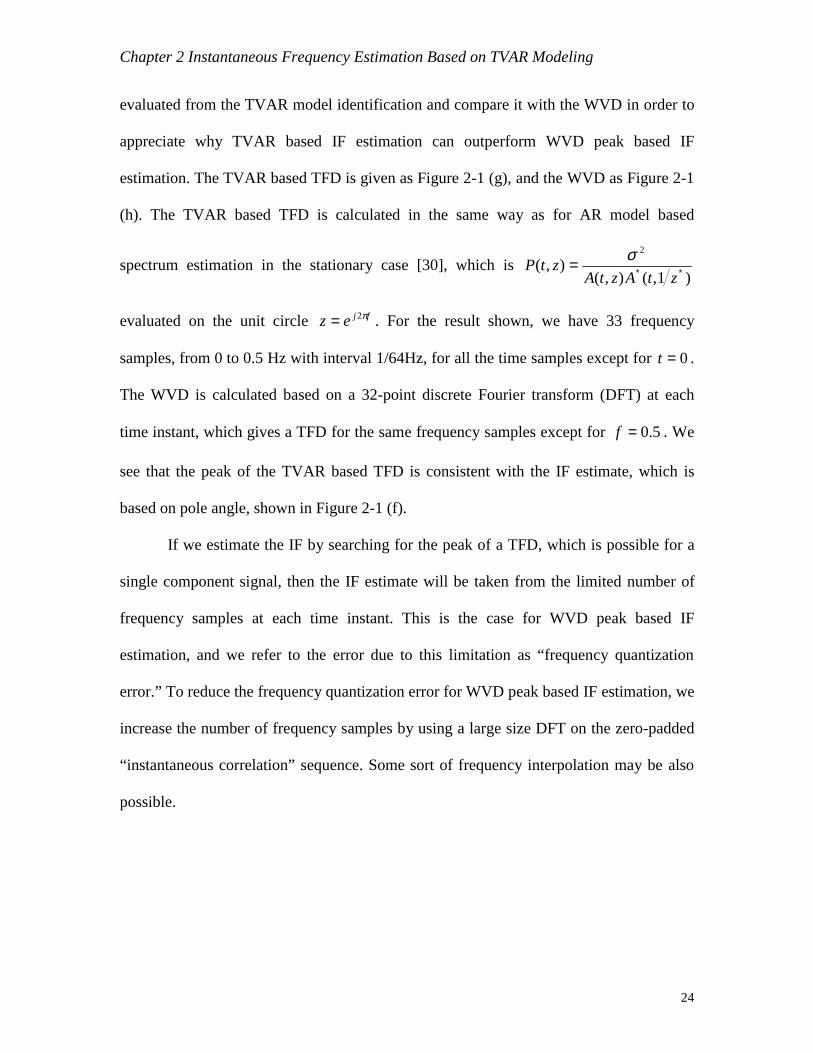
24
evaluated from the TVAR model identification and compare it with the WVD in order to
appreciate why TVAR based IF estimation can outperform WVD peak based IF
estimation. The TVAR based TFD is given as Figure 2-1 (g), and the WVD as Figure 2-1
(h). The TVAR based TFD is calculated in the same way as for AR model based
spectrum estimation in the stationary case [30], which is )1,(),(
),(2
∗∗=ztAztA
ztPσ
evaluated on the unit circle fjez π2= . For the result shown, we have 33 frequency
samples, from 0 to 0.5 Hz with interval 1/64Hz, for all the time samples except for 0=t .
The WVD is calculated based on a 32-point discrete Fourier transform (DFT) at each
time instant, which gives a TFD for the same frequency samples except for 5.0=f . We
see that the peak of the TVAR based TFD is consistent with the IF estimate, which is
based on pole angle, shown in Figure 2-1 (f).
If we estimate the IF by searching for the peak of a TFD, which is possible for a
single component signal, then the IF estimate will be taken from the limited number of
frequency samples at each time instant. This is the case for WVD peak based IF
estimation, and we refer to the error due to this limitation as “frequency quantization
error.” To reduce the frequency quantization error for WVD peak based IF estimation, we
increase the number of frequency samples by using a large size DFT on the zero-padded
“instantaneous correlation” sequence. Some sort of frequency interpolation may be also
possible.

Chapter 2 Instantaneous Frequency Estimation Based on TVAR Modeling
25
( a ) ( b )
( c ) ( d )
Figure 2-1. An example of TVAR based IF estimation from a complex-valued data record taken from an analytical linear FM signal in complexwhite noise, with 1=p and 3=q for the TVAR model (continued on thenext page):( a ) the IF law used to generate the data,( b ) the estimated TVAR coefficient 31,,2,1),(1 �=tta , in terms of its real
(solid) and imaginary part (dashed),( c ) the real parts of the data (solid) and the TVAR 1-step prediction
(dashed),( d ) the imaginary parts of the data (solid) and the TVAR 1-step prediction
(dashed).

Chapter 2 Instantaneous Frequency Estimation Based on TVAR Modeling
26
( e ) ( f )
time
frequ
ency
0 10 20 300
0.1
0.2
0.3
0.4
0.5
time
frequ
ency
0 10 20 300
0.1
0.2
0.3
0.4
0.5
( g ) ( h )
Figure 2-1. (continued) An example of TVAR based IF estimation, acomplex-valued data record with an analytical linear FM signal incomplex white noise, 1=p and 3=q for the TVAR model:( e ) the trajectory of the estimated time-varying pole of the TVAR model,( f ) IF estimate based on TVAR model (solid) vs. the exact IF (dashed),( g ) the time-varying spectrum evaluated from the TVAR model,( h ) the WVD of the data record.
In calculating the WVD estimate, a smaller and smaller number of data samples is
available when estimating the instantaneous correlation function for a time instant near

Chapter 2 Instantaneous Frequency Estimation Based on TVAR Modeling
27
the ends of the data record. Consequently, the peak of the WVD fades out towards the
ends of the data record, as shown in Figure 2-1 (h). The latter will lead to very poor IF
estimation near the ends of a data record. This limitation is referred to as “end effects” for
the WVD peak based IF estimation.
Another drawback of TFD peak based IF estimation is that it requires calculating
and storing the 2-dimensional distribution, the TFD, and 1-dimensional peak searching
on the TFD. This could be a major implementation burden in terms of computing power
and memory size. Another reason that we use the pole angle, rather than the location of
the spectral (TFD) peak, derives from the analogy of TVAR based IF estimation to AR
spectral estimation. For AR model based frequency (tone) estimation in the stationary
case, pole angle based estimation was shown to lead to better performance than spectral
peak based estimation [30].
2.2.3 Example 2: A Frequency-Hopping Signal
As another example, we demonstrate the TVAR based IF estimation approach on
a record of a frequency-hopping signal. Here we consider a frequency-hopping signal
with 32 samples at unit sampling rate. The IF hops from 0.1 to 0.3 Hz at 20=t , as
plotted in Figure 2-2 (a). As in Example 1, the signal is corrupted by additive white
Gaussian noise at SNR=20dB. A complex-valued data record is generated, as shown with
solid lines in Figure 2-2 (c), for the real part, and in Figure 2-2 (d), for the imaginary part.
We model the data record with a TVAR model with 1=p and 5=q , and use
polynomials as the set of “basis functions” qktuk ,,1,0),( �= to represent the TVAR
coefficients )(tai . This is similar to Example 1 except for a difference in the polynomial

Chapter 2 Instantaneous Frequency Estimation Based on TVAR Modeling
28
order. The estimated )(1 ta is shown in Figure 2-2 (b). The TVAR one-step prediction is
plotted against the data in Figure 2-2 (c) for the real part and in Figure 2-2 (d) for the
imaginary part. We observe a close match between the data and the prediction.
Now we find the time-varying pole )()( 11 tatp −= . The trajectory of the pole is
shown in Figure 2-2 (e) by the “+” marks. The IF estimate is then obtained by evaluating
the angle of the pole at each time instant. In Figure 2-2 (f), the IF estimate (solid) is
compared against the exact IF (dashed). The TVAR model using the 5th order
polynomial follows the frequency hopping successfully.
As in Example 1, we now examine the time-varying spectrum, evaluated from the
identified TVAR model, and compare it with the WVD. The TVAR based TFD is given
in Figure 2-2 (g), and the WVD in Figure 2-2 (h). The TVAR based TFD is consistent
with the IF estimate. For the WVD, we can see the end-effects and the severe pseudo
peaks due to cross-term interference.
2.3 Performance of TVAR Based IF Estimation
In this section, we evaluate the performance of the TVAR based IF estimation by
comparing it through simulations with the WVD based IF estimation and the Cramer-Rao
bound [31,62]. We first compare the TVAR based method with the WVD based method
for a case of a linear FM signal since the WVD method had been shown to be optimal for
such cases at high to moderate SNR. We then examine a more general case with a
nonlinear IF law.
Chapter 2 Instantaneous Frequency Estimation Based on TVAR Modeling
29
( a ) ( b )
( c ) ( c )
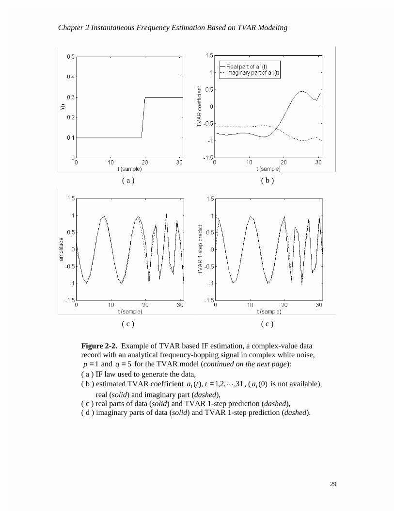
Figure 2-2. Example of TVAR based IF estimation, a complex-value datarecord with an analytical frequency-hopping signal in complex white noise,
1=p and 5=q for the TVAR model (continued on the next page):( a ) IF law used to generate the data,( b ) estimated TVAR coefficient 31,,2,1),(1 �=tta , ( )0(ia is not available),
real (solid) and imaginary part (dashed),( c ) real parts of data (solid) and TVAR 1-step prediction (dashed),( d ) imaginary parts of data (solid) and TVAR 1-step prediction (dashed).

Chapter 2 Instantaneous Frequency Estimation Based on TVAR Modeling
30
( e ) ( f )
time
frequ
ency
0 10 20 300
0.1
0.2
0.3
0.4
0.5
time
frequ
ency
0 10 20 300
0.1
0.2
0.3
0.4
0.5
( g ) ( h )
Figure 2-2. (continued) An example of TVAR based IF estimation, a complex-value data record with an analytical frequency-hopping signal in complex whitenoise, 1=p and 5=q for the TVAR model:( e ) trajectory of the estimated time-varying pole of the TVAR model,( f ) IF estimate based on TVAR model (solid) vs. the exact IF (dashed),( g ) time-varying spectrum evaluated from the TVAR model,( h ) the WVD of the data record.

Chapter 2 Instantaneous Frequency Estimation Based on TVAR Modeling
31
2.3.1 Experiment Setup and Implementation
In the simulation experiments, we consider a short data record of 32 samples. The
data consists of an FM signal, linear or nonlinear, and additive white Gaussian noise. In
generating the FM signal, the FM law is set as deterministic, while the initial phase is
random (uniform over [0,2π)), and varies from trial to trial in the simulation.
We use complex-valued data representing an analytical FM signal in complex
noise, rather than real-valued data. In practice, the complex-valued data could be analytic
if it is obtained through Hilbert transformation from real-valued data. Nevertheless, here
we consider the more general case where the signal part is analytic, while the noise part is
not, and has double-sided non-symmetric spectrum. Using complex-valued data enables
us to use a lower autoregressive order for the TVAR model, which implies simplicity in
implementation. For the WVD based IF estimation method it is also necessary to use
complex-valued data with an analytic signal component to avoid frequency aliasing of the
signal component in the time-frequency plane.
In our implementation of the TVAR parameter estimation, the set of generalized
covariance equations, of size )1( +qp , is solved simply using Gaussian elimination.
While fast algorithms are available [29, 63, 64], these are beyond the topic of this
research. To calculate the WVD for each data record of length 32, 32-point (without zero-
padding) or, for example, 4096-point (with zero-padding) DFT’s are performed for each
time instant. The DFT at each time instant is performed on the “instantaneous auto-
correlation” sequence, which computes the “instantaneous power distribution” for that
time instant. In calculating the “instantaneous auto-correlation” sequence, zero values are
assumed outside of the data record.

Chapter 2 Instantaneous Frequency Estimation Based on TVAR Modeling
32
The IF estimation errors at each time instant are calculated by comparing the IF
estimates with the exact IF value that was used to generate the data. The mean square
error (MSE) of the IF estimation is estimated by averaging the squared IF errors across
both time instants and simulation trials. Two ranges of time instants are used to evaluate
the MSE of IF estimation: the 16 time instants near the time center of the data record, and
the full time duration except the first p (the autoregressive order) instants, where the
TVAR based IF estimates are not available. As a measure of IF estimation performance,
the reciprocal of the estimated MSE, 1/MSE, is plotted versus SNR.
2.3.2 Linear FM Signal Scenarios
As shown in Figure 2-1, we use a linear FM signal with 32 samples at unit
sampling rate, which chirps in frequency from 0.1 to 0.41 Hz according to
31,,1,0,01.01.0)( �=+= tttf , and is corrupted by additive white Gaussian noise. The
signal is generated using the IF with unit amplitude and a random initial phase. The
reason for choosing a linear FM signal is that the WVD peak based IF estimator is
optimal for this type of signal at high to moderate SNR [31, 33]. The analytic signal in
complex-valued noise is used. The model involved is a first-order autoregressive model
(p=1) with the time-varying coefficient represented as a third-order polynomial function
(q=3), denoted as TVAR(1,3). The generalized covariance method [28] is used to identify
the TVAR parameters.

Chapter 2 Instantaneous Frequency Estimation Based on TVAR Modeling
33
Figure 2-3. 1/MSE vs. SNR on the full time duration: TVAR-IF (solid)and WVD-IF (dotted).
In Figure 2-3, the reciprocal of the MSE is plotted against SNR, for both TVAR
based and WVD peak based IF estimation. We ran 100 simulation trials for each SNR
value and the MSE was calculated from the 100 IF estimates at samples t from 1 to 31. In
this case, the TVAR based method outperforms the WVD based method and the end-
effects of the WVD calculation produce a distinct performance ceiling for the WVD
based IF estimates. The end-effects are due to the fact that, with finite-length data
records, the number of data samples involved in calculating the discrete WVD is
proportional to the distance from the closest end of the data record.
Next, we compare the two methods without the influence of the end-effects. The
MSE of the IF estimates is evaluated for the time indices t=8 through 23, i.e. during the
central half of the data record. The results are shown in Figure 2-4. While the TVAR
based estimation did not change appreciably, the WVD based estimation performs

Chapter 2 Instantaneous Frequency Estimation Based on TVAR Modeling
34
significantly better away from the ends of the data record. However, another performance
ceiling materializes for WVD based IF estimation at SNR above 6dB. This ceiling is due
to the frequency quantization error of the discrete WVD arising from the finite length of
the data records. For 32-sample sequences, the time-frequency bins for the discrete WVD
are of the size of 1 sample period in time by 0.5/32=1/64 Hz in frequency, if no zero-
padding is applied.
Figure 2-4. 1/MSE vs. SNR near the time center of the data record:TVAR-IF (solid) and WVD-IF peak (dotted).
When using WVD based IF estimation, for short records with moderate to high
SNR, the associated frequency quantization error dominates the IF estimation error at the
center of the data record, while the end-effects of the WVD calculation produce
estimation errors that dominate the overall IF estimation performance. In comparison,
TVAR based IF estimation is free of the frequency quantization error and its end-effects
are slight. Here we chose the WVD peak based IF estimator to compare against, but our

Chapter 2 Instantaneous Frequency Estimation Based on TVAR Modeling
35
conclusion may be generalized to other time-frequency distribution (TFD) peak or
moment based IF estimators [31].
The results are consistent for various lengths of data records at high SNR. Figure
2-5 shows the simulation of 1/MSE versus number of samples N with SNR=20dB. For
different N, we use similar linear FM signals with N samples at unit sampling rate, which
chirp in frequency from 0.1 to 0.41~0.42 Hz according to tN
tf32
01.01.0)( += ,
1,,1,0 −= Nt � .
Figure 2-5. 1/MSE vs. number of samples N near the time center of thedata record, SNR=20dB: TVAR-IF (solid) and WVD-IF (dotted).
To reduce the frequency quantization error, interpolation on the discrete WVD or
zero-padding on the WVD kernel [33] or data is necessary. In this way the WVD based
IF estimator may approach the optimal performance, i.e. the Cramer-Rao bound (CRB)
for linear FM [31,61,62], at the center of the data record, as given by
)1()()2(
12]ˆvar[
222 −≥
NNAf
σπ(2-3)

Chapter 2 Instantaneous Frequency Estimation Based on TVAR Modeling
36
where N is the number of samples, A is the signal amplitude, and 2σ is the noise
variance. Figure 2-6 shows the simulation result for IF estimates at the center half of the
data records (samples t=8~23) when zeros are padded so that a 4096-point DFT is used in
calculating the WVD, rather than the 32-point DFT used earlier. At moderate to high
SNR, the MSE of the TVAR based estimator is about 10dB higher than the Cramer-Rao
bound.
Figure 2-6. 1/MSE vs. SNR near the time center of the data record:TVAR-IF (solid), WVD-IF (dotted) with sufficient zero-padding, and theCramer-Rao Bound (dashed).
2.3.3 Non-Linear FM Signal Scenarios
Now, we compare TVAR and WVD based IF estimators in the case of a nonlinear
FM signal scenario. This simulation is the same as in the linear FM case except that here
the desired IF law is 20004.005.0)( ttf += , 31,,1,0 �=t . Considering the higher order
of the IF law, we increased the AR coefficient order to q=5. Zero-padding to 4096 points

Chapter 2 Instantaneous Frequency Estimation Based on TVAR Modeling
37
is applied in the WVD method so that the effect of frequency quantization error is
virtually removed. The 1/MSE results are plotted versus SNR in Figure 2-7, which
represents IF estimation at the center half of the time record.
Figure 2-7. 1/MSE vs. SNR near the time center of the data record for anonlinear FM signal: TVAR-IF (solid) with q=5, and WVD-IF peak(dotted) with zero-padding to 4096 points.
Comparing Figure 2-7 and Figure 2-6, the TVAR based method performs about
the same as in the linear FM case while the WVD based method degrades noticeably.
This means that the TVAR based method is significantly less sensitive to the nonlinearity
of the IF law. The new performance ceiling of the WVD method in Figure 2-7 is due to
the bias of the WVD based IF estimation. That is, when the IF law is not ideally linear,
the peak of the WVD shifts away from the position of the actual instantaneous frequency.
Selecting a higher order q for TVAR based IF estimation, such as q=5 in Figure
2-7, reduces the AR coefficient fitting error which dominates the performance at high

Chapter 2 Instantaneous Frequency Estimation Based on TVAR Modeling
38
SNR, but also accommodates more noise into the model which dominates the
performance at low SNR. Figure 2-8 gives the performance of the TVAR-IF method
when selecting the order q=3. Here the 1/MSE of the TVAR method increases slowly
with SNR due to the AR coefficient fitting error, but it is about 4 dB higher at low SNR
than when using q=5.
Figure 2-8. 1/MSE vs. SNR near the time center of data record for a nonlinearFM signal: TVAR-IF (solid) with q=3, and WVD-IF (dotted).
Figure 2-9 helps to observe and explain the performance degradation of the WVD
based method for the nonlinear IF law. In Figure 2-9, we show the actual IF and 100
trials of IF estimation based on the WVD (with enough zero-padding) at each instant, for
SNR=20 dB. Besides the end-effects, which produce significant IF estimation variance
near the ends of the data record, we also see that the WVD based IF estimation is
severely biased toward the inner side of the IF curve.

Chapter 2 Instantaneous Frequency Estimation Based on TVAR Modeling
39
Figure 2-9. Exact IF (solid line) and WVD based 100 trials of estimates(discrete points) at each instant, for SNR=20 dB, using the WVD peakbased IF estimator with zero-padding to length 4096.
In summary, the TVAR based IF estimator is a fairly good one, and especially
advantageous for those practical cases where only a short data record is available and
linear IF laws can not be assumed a priori. The optimality of the WVD based method
requires the following simultaneous conditions: 1) a linear FM signal, 2) the time
instances of the estimated IF are far from the ends of the data record, 3) generous zero-
padding or frequency interpolation, and 4) high SNR. Violation of any of the conditions
can make the WVD based method perform worse than the TVAR based method. The
TVAR based method, though not optimal in any case, is more robust and performs
satisfactorily in various situations. In addition, the benefit of the TVAR based method
being cross-term free is highly desired for signals consisting of multiple closely spaced
FM components.

Chapter 2 Instantaneous Frequency Estimation Based on TVAR Modeling
40
2.4 Summary
In this chapter, we introduced the TVAR based IF estimation method with a
detailed example, and then examined the performance of the TVAR based IF estimation
method through simulations. The results suggested that it is worthwhile to further study
this method. In the next chapter, we will propose a time-varying Prony method to
improve the TVAR based method for noisy data and lower SNR. Convinced by the
results in this chapter, we will apply the TVAR based IF estimation to communication
interference cancellation in Chapter 4.

Chapter 3 A Time-Varying Prony Method for IF Estimation at Low SNR
41
Chapter 3
A TIME-VARYING PRONY METHOD FOR IF
ESTIMATION AT LOW SNR
In this chapter, we propose a time-varying Prony method to improve the TVAR
based IF estimation performance at low SNR. The benefit of the method is evidenced
through simulations. Part of the work in this chapter was published earlier [65].
3.1 Introduction
Instantaneous frequency (IF) estimation for frequency modulated (FM) signals in
white noise is a classical problem. The available methods range from the classical zero-
crossing counting and phase-lock-loop (PLL) to recently developed time-frequency
distribution (TFD) based methods [31]. In high signal-to-noise ratio (SNR) environments,
many methods yield accurate IF estimates and even reach the Cramer-Rao bound in some
situations, whereas most of these methods deteriorate dramatically when SNR falls below
some threshold [31].

Chapter 3 A Time-Varying Prony Method for IF Estimation at Low SNR
42
Time-varying autoregressive (TVAR) model based IF estimation had been
considered poor since being proposed in 1984 by Sharman and Friedlander [36,31]. Shan
and Beex [34], as reported in Chapter 2, have recently shown that the TVAR method is
fairly good, and especially advantageous for those practical cases where short data
records are used or linear IF law can not be assumed a priori. This is further evidenced
by the improved system performance provided by the TVAR based method when applied
to interference cancellation in spread spectrum communications [57].
On the other hand, our results in Chapter 2 also revealed that, similar to other IF
estimation methods [31], the reciprocal of MSE of the TVAR based IF estimation falls
faster after the SNR falls below some value. In this chapter, we focus on improving the
TVAR-IF method for low SNR environments.
In stationary cases, sinusoids in white noise can be approximately modeled as an
AR process, and the frequencies can be estimated from the model. This AR model based
frequency estimation method is referred to as the Prony method [30, 53]. At low SNR,
the eigen-structure of the data correlation matrix can be exploited to improve frequency
estimation precision significantly [30]. An alternative, less complicated, method to solve
this problem was proposed by Kumaresan, Tufts, and Scharf [53]. The performance of
this alternative approach was shown to be “close to that of the best available, more
complicated, approaches which are based on maximum likelihood or on the use of
eigenvector or singular value decompositions” [53].
We extend this less complicated low-SNR Prony method to time-varying cases to
improve the TVAR based IF estimation at low SNR. First, the autoregressive order is set
higher than that needed for pure signal components so that the extra poles capture part of

Chapter 3 A Time-Varying Prony Method for IF Estimation at Low SNR
43
the noise. Then we choose “signal poles” based on a subset selection procedure.
Simulations show significant improvement of the IF estimation, especially when SNR is
low.
3.2 A Time-Varying Prony Method: Method and Example
3.2.1 Method
For a signal consisting of M FM components in white noise at low to moderate
SNR, we model the signal with a TVAR model, with order p>M for complex exponential
FM components and p>2M for real-valued signals. M is assumed known here. For the
sake of presentation, in the rest of this section we assume to be using complex data,
consisting of an analytic signal in complex noise.
As in the case of high SNR, the time-varying transfer function corresponding to
the TVAR model can be expressed by (2-1). By rooting the denominator polynomial
formed by the TVAR coefficient estimates at each time instant t , we obtain the p poles as
functions of time: pitpi ,,2,1),( �= . With order p>M for the low SNR case, among the
p pole trajectories, there are M signal pole trajectories and (p-M) noise pole trajectories.
The trajectories associated with the FM components tend to be along the unit circle while
the poles capturing the noise move wildly, mostly inside, but occasionally outside
(especially near the ends of a data record) the unit circle.
The instantaneous angles of the pole trajectories associated with the FM
components can be used as estimates of the instantaneous frequencies )(tf i . The key
problem here is to find, at each instant t, the best subset of the poles as the M signal poles.

Chapter 3 A Time-Varying Prony Method for IF Estimation at Low SNR
44
Our objective is to find, at each moment, the best subset of size M out of the p poles so
that the M trajectories formed from the subsets provides the least total squared prediction
error over the entire data record. For data size N, we have pN
M
p−
potential
combinations to choose from. Although we may use, for example, the Viterbi algorithm
to solve this combinatorial optimization problem, it is desirable to have a less
complicated way to find a subset of poles to improve the IF estimation for low SNR
environments.
To meet this demand, we suggest a subset selection method that is based on the
instantaneous squared prediction error. At time t, the autoregressive coefficients
associated with a pole subset, denoted as ψ, of size M, are determined by
])(1[)( 1
0
−
∈=
− ∏∑ −= ztpztam
m
M
i
ii
ψ
ψ (3-1)
Then the squared prediction error at time t corresponding to the subset ψ is
2
1
)()()()( ∑=
−−=M
ii itxtatxt ψψε (3-2)
At each time instant t, we choose the subset that gives the smallest )(tψε . We refer to
this criterion as the instantaneous least squares (ILS) criterion.
At each time instant, there are
M
p possible subsets of size M. For small M and
p, the desired subset can be easily determined by comparing all possible subsets. For
cases of large M and p, the procedure of Hocking and Leslie [56] can be used to simplify
the subset selection, as suggested by Kumaresan, Tufts, and Scharf for the stationary case
[53]. In the latter procedure, the significance of each pole is evaluated in terms of the

Chapter 3 A Time-Varying Prony Method for IF Estimation at Low SNR
45
prediction error increment after removing the pole from the entire set of p poles. All poles
are sorted according to the significance measure, and from this ordering, a sub-best
subset can be selected without exhausting all the possible combinations.
3.2.2 Example
Now we present an example to illustrate the proposed method. We use a noisy
short data record with 32 samples at unity sampling rate. The data is complex-valued, and
consists of a complex exponential function with time-varying frequency and additive
complex Gaussian white noise. For the complex exponential signal part, we need one
pole (M=1). For the proposed time-varying Prony method, to have an extra pole to
capture some of the noise, we set the autoregressive order equal to two (p=2). The
polynomial basis is used to represent the TVAR coefficients and the polynomial order is
set, quite arbitrarily, equal to four (q=4). The proposed instantaneous least squares (ILS)
criterion for subset selection is used to determine the signal pole at each time instant.
The example to be presented is for highly nonlinear FM at the low SNR of 3dB.
The data is generated with a random initial phase and unity amplitude, and the IF varies
between 0.1 and 0.4Hz (normalized to sampling rate) according to
)32
sin(3.01.0)(t
tfπ+= , 31,,1,0 �=t . The real part and the imaginary part of the data
sequence are plotted in Figure 3-1 (a). The proposed method, which uses autorgeressive
order p=2 and the ILS criterion, is hereafter referred to as “TVAR(2)+ILS”, for
simplicity. The TVAR based IF estimation method for high SNR, studied in Chapter 2,
which uses autoregressive order p=1 is referred to as “TVAR(1).” To demonstrate the

Chapter 3 A Time-Varying Prony Method for IF Estimation at Low SNR
46
improvement of the proposed method we evaluate the performance of both methods and
show them side by side.
( a ) ( b )
( c ) ( d )
Figure 3-1. An example of IF estimation at low SNR for a highly non-linear FMat SNR=3dB (continued on the next page):( a ) real (solid) and imaginary part (dashed) of data,( b ) trajectory of pole radius for TVAR(1),( c ) trajectory of pole radii for TVAR(2),( d ) trajectory of signal pole radius as determined by TVAR(2) + ILS.

Chapter 3 A Time-Varying Prony Method for IF Estimation at Low SNR
47
( e ) ( g )
( g )
Figure 3-1. (continued) An example of IF estimation at low SNR, for a highlynon-linear FM at SNR=3dB:( e ) TVAR(1), IF estimate (dashed) vs. the exact IF (solid),( f ) TVAR(2) + ILS, IF estimate (dashed) vs. the exact IF (solid),( g ) The WVD (zeros padded to 256 points) peak based IF estimate (dashed) vs.
the exact IF (solid).
As expected, the TVAR based IF estimation without subset selection, TVAR(1),
performs poorly in the low SNR case. The noise forces the pole trajectory away from the
unit circle, as shown by Figure 3-1 (b), and the resulting IF estimate is poor, as given by
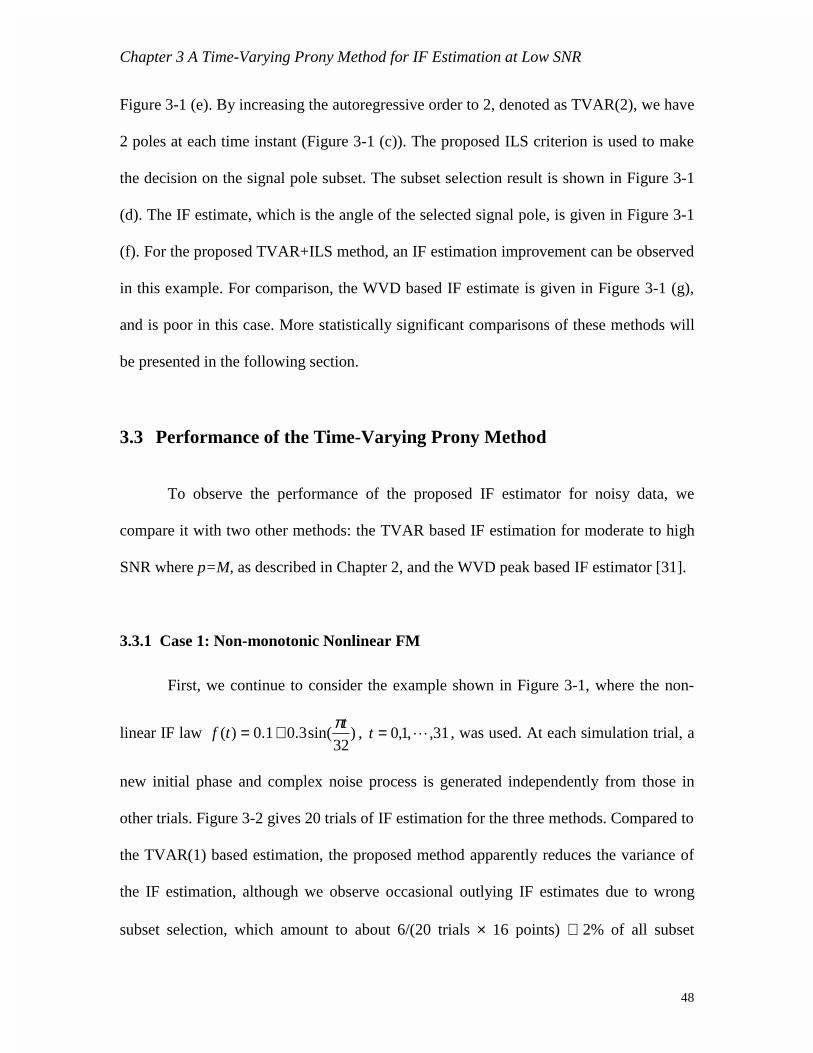
Chapter 3 A Time-Varying Prony Method for IF Estimation at Low SNR
48
Figure 3-1 (e). By increasing the autoregressive order to 2, denoted as TVAR(2), we have
2 poles at each time instant (Figure 3-1 (c)). The proposed ILS criterion is used to make
the decision on the signal pole subset. The subset selection result is shown in Figure 3-1
(d). The IF estimate, which is the angle of the selected signal pole, is given in Figure 3-1
(f). For the proposed TVAR+ILS method, an IF estimation improvement can be observed
in this example. For comparison, the WVD based IF estimate is given in Figure 3-1 (g),
and is poor in this case. More statistically significant comparisons of these methods will
be presented in the following section.
3.3 Performance of the Time-Varying Prony Method
To observe the performance of the proposed IF estimator for noisy data, we
compare it with two other methods: the TVAR based IF estimation for moderate to high
SNR where p=M, as described in Chapter 2, and the WVD peak based IF estimator [31].
3.3.1 Case 1: Non-monotonic Nonlinear FM
First, we continue to consider the example shown in Figure 3-1, where the non-
linear IF law )32
sin(3.01.0)(t
tfπ+= , 31,,1,0 �=t , was used. At each simulation trial, a
new initial phase and complex noise process is generated independently from those in
other trials. Figure 3-2 gives 20 trials of IF estimation for the three methods. Compared to
the TVAR(1) based estimation, the proposed method apparently reduces the variance of
the IF estimation, although we observe occasional outlying IF estimates due to wrong
subset selection, which amount to about 6/(20 trials × 16 points) ≅ 2% of all subset
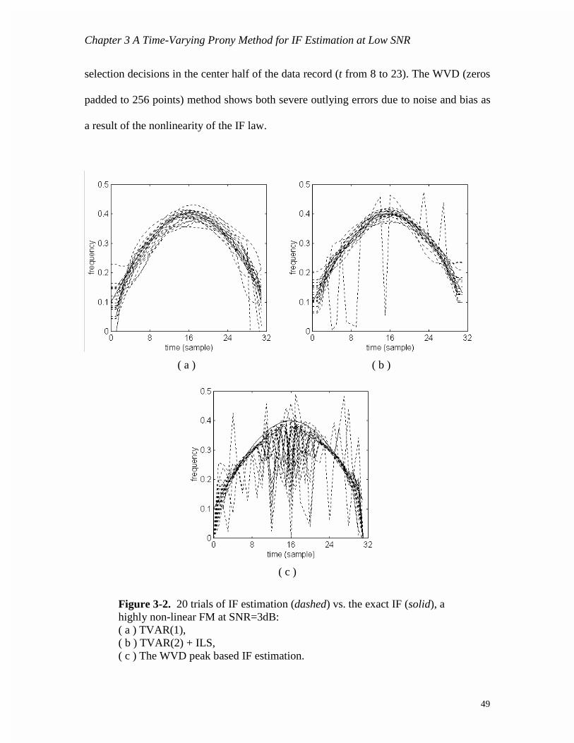
Chapter 3 A Time-Varying Prony Method for IF Estimation at Low SNR
49
selection decisions in the center half of the data record (t from 8 to 23). The WVD (zeros
padded to 256 points) method shows both severe outlying errors due to noise and bias as
a result of the nonlinearity of the IF law.
( a ) ( b )
( c )
Figure 3-2. 20 trials of IF estimation (dashed) vs. the exact IF (solid), ahighly non-linear FM at SNR=3dB:( a ) TVAR(1),( b ) TVAR(2) + ILS,( c ) The WVD peak based IF estimation.

Chapter 3 A Time-Varying Prony Method for IF Estimation at Low SNR
50
To further examine the performance of the proposed method, we run 1000
simulation trials and the IF estimation errors in the center half of the data record (t from 8
to 23) are evaluated. The result is shown in Figure 3-3 in terms of the reciprocal of the
mean squared error (MSE) of IF estimation, 1/MSE, versus SNR. Noticeable
performance improvement is achieved for SNR below 3dB. In Figure 3-3, there is no
noticeable improvement in 1/MSE at 3dB SNR, unlike what Figure 3-2 may suggest.
This is due to the outlying errors with the proposed method. In spite of this, the
improvement is significant for SNR near or below 0dB. The WVD method performs
poorly even at higher SNR in this case due to its biased estimation, as evidenced in
Figure 3-2.
Figure 3-3. 1/MSE vs. SNR for IF estimation near the time center of thedata record for a highly nonlinear FM signal.
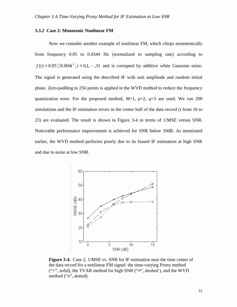
Chapter 3 A Time-Varying Prony Method for IF Estimation at Low SNR
51
3.3.2 Case 2: Monotonic Nonlinear FM
Now we consider another example of nonlinear FM, which chirps monotonically
from frequency 0.05 to 0.4344 Hz (normalized to sampling rate) according to
2004.005.0)( ttf += , 31,,1,0 �=t and is corrupted by additive white Gaussian noise.
The signal is generated using the described IF with unit amplitude and random initial
phase. Zero-padding to 256 points is applied in the WVD method to reduce the frequency
quantization error. For the proposed method, M=1, p=2, q=3 are used. We run 200
simulations and the IF estimation errors in the center half of the data record (t from 16 to
23) are evaluated. The result is shown in Figure 3-4 in terms of 1/MSE versus SNR.
Noticeable performance improvement is achieved for SNR below 10dB. As mentioned
earlier, the WVD method performs poorly due to its biased IF estimation at high SNR
and due to noise at low SNR.
Figure 3-4. Case 2, 1/MSE vs. SNR for IF estimation near the time center ofthe data record for a nonlinear FM signal: the time-varying Prony method(“+”, solid), the TVAR method for high SNR (“×”, dashed ), and the WVDmethod (“o”, dotted).

Chapter 3 A Time-Varying Prony Method for IF Estimation at Low SNR
52
3.3.3 Case 3: Linear FM
We now use 32 samples of a linear FM signal, which chirps from frequency 0.1 to
about 0.4 Hz according to ttf 01.01.0)( += , 31,,1,0 �=t . Otherwise, the experiment is
the same as in the nonlinear FM cases. The result is shown in Figure 3-5. Again,
noticeable performance improvement is achieved for SNR below 10dB. The WVD
method is potentially optimal for this case due to pure linearity of the FM law [31,34].
The optimality of the WVD method materializes when SNR is above 6dB. However, at
lower SNR (below 3dB for this example), the proposed TVAR+ILS method provides the
best estimation among the three methods.
Figure 3-5. Case 3, 1/MSE vs. SNR for IF estimation near the time centerof the data record for a linear FM signal: the time-varying Prony method(“+”, solid), the TVAR method for high SNR (“×”, dashed ), and theWVD method (“o”, dotted).

Chapter 3 A Time-Varying Prony Method for IF Estimation at Low SNR
53
3.4 Summary
Most available instantaneous frequency estimation methods for FM signals in
white noise deteriorate dramatically when SNR falls below some threshold. In this
chapter, we proposed a time-varying Prony method for IF estimation from low SNR data.
It is an extension of a frequency estimation method for stationary processes which was
shown to be less complicated, yet close in performance to the best available approaches
based on singular value decomposition or the principle of maximum likelihood. First, the
time-varying autoregressive order is set higher than that needed for the pure signal
components, so that the extra poles capture part of the noise. Then we choose “signal
poles” based on a subset selection procedure. The performance improvement at low SNR
over the TVAR method for high SNR is evidenced through simulation experiments. The
proposed method also outperforms the “optimal” WVD method, when it loses optimality
for low SNR scenarios.

Chapter 4 Notch Filter Based Interference Suppression Using TVAR Based IF Estimation
54
Chapter 4
NOTCH FILTER BASED INTERFERENCE
SUPPRESSION USING TVAR BASED IF
ESTIMATION
In case of strong frequency modulated (FM) interference in a spread spectrum
communication system, the interference can be effectively suppressed by applying a
time-varying notch filter with its zero(s) placed at an instantaneous frequency (IF)
estimate of the interference. As we mentioned in Chapter 1, the published studies use
Wigner-Ville distribution (WVD) peak based IF estimation. In this chapter, we study the
use of the time-varying autoregressive (TVAR) model based IF estimator of Chapter 2 in
such a scenario. It is demonstrated that the TVAR-IF method provides improved
performance compared to using the WVD based method. It is also shown that the TVAR
method is capable of handling multiple component interference without separation into
individual components. A major part of this work was published earlier [57].

Chapter 4 Notch Filter Based Interference Suppression Using TVAR Based IF Estimation
55
4.1 Introduction
The problem of frequency modulated (FM) interference suppression in direct-
sequence spread spectrum (DSSS) communications has been attracting many researchers
recently [48-50,58]. Amin and his colleagues, Lach and Lindsey, studied methods using
time-frequency distributions (TFD): time-varying notch filtering using an instantaneous
frequency (IF) estimated from a TFD [48], time-frequency filtering through signal
synthesis after masking of the TFD, specifically the Wigner-Ville distribution (WVD)
[49], and a comparison of the two approaches [58]. Bultan and Akansu [50] used the
iterative matching pursuit algorithm with a chirplet dictionary to detect and excise chirp-
like interference. Wei, Harding, and Bovik [59] used an iterative time-frequency filtering
algorithm based on masking of the Gabor transform followed by signal synthesis.
All the aforementioned filtering procedures are highly non-causal, and require
data-block based time-frequency analysis before signal synthesis or linear filtering. For
practical system implementation, the associated computation and memory requirements
have to be controlled to an acceptable amount. This suggests that the entire filtering
procedure be either implemented in a data-recursive form or perform well with short data
blocks. Similar to stationary cases, an appropriate parametric method - with a priori
information exploited - would perform better than those non-parametric methods that are
based on TFDs, such as the WVD or other members of the Cohen class of time-frequency
distributions. This is one of the reasons that we study FM interference suppression using
parametric IF estimation. Another reason is that WVD based IF estimation is not
appropriate for non-linear FM laws due to the associated bias problem, as shown in
Chapter 2. In contrast, the parametric method we studied is not sensitive to non-linearity

Chapter 4 Notch Filter Based Interference Suppression Using TVAR Based IF Estimation
56
of IF laws, is suitable for short data blocks, is free of frequency quantization and cross-
terms, and produces lesser end effects [34].
We model the received signal consisting of an FM interference (single FM or
multiple FM) thermal noise and DSSS signal with a time-varying autoregressive (TVAR)
model. The IF of the interference is estimated from the model and then a notch filter is
formed according to the IF estimate.
4.2 Notch filter Based FM Interference Suppression Using TVAR
Based IF Estimation
At the receiver of a DSSS communications system, an interference suppression
filter is applied before demodulation. We consider a received signal )(tr composed of the
DSSS signal )(ts , thermal noise )(tw , and interference )(ti :
)(tr = )(ts + )(tw + )(ti (4-1)
Here the noise )(tw is assumed stationary and white. The DSSS signal )(ts is “slightly
colored” in practice, which depends on the sampling rate (samples per chip) as well as the
specific PN sequence. The FM interference )(ti could be an intentional or unintentional
jammer, such as a strong FM communication emitter. The components in (4-1) are
assumed mutually independent.
In the stationary case, tones in white noise can be modeled as an AR process and
the frequencies of the tones can be estimated from AR modeling. We can model the
received signal )(tr with a time-varying AR model, viewed as an FM in white noise
process, if we treat the DSSS signal as approximately white. The IF of the FM

Chapter 4 Notch Filter Based Interference Suppression Using TVAR Based IF Estimation
57
interference )(ti is estimated as described in Chapter 2. Then )(tr is fed into a time-
varying filter ),( tzN to suppress the interference. The filter ),( tzN is a time-varying
notch filter with its zeros placed at the IF estimate. A study of the design and
performance issues of this filter can be found elsewhere [60]. The block diagram of the
receiver (BPSK modulation assumed) with an IF based interference suppression filter is
given in Figure 4-1.
Down-convert
to baseband
Sampler
FM interferenceDSSS signal
RF front-end
thermalnoise
Inst. Freq.estimator
Notchfilter
N (z, t)
r(t) y(t)
Despreadingsequence
Sum over each bitinterval
Bitdecision
PN code
Interferencesuppression
BPSK DSSS demodulator
Databuffer
Figure 4-1. Block diagram of the DSSS receiver with IF estimation basedFM interference suppression.
4.3 System Performance Improvement Due to Interference Rejection
Using TVAR Based IF Estimation
In this section, we examine the system performance improvement due to the notch
filter based interference rejection using the TVAR based IF estimation. We will compare
the overall system performance with the notch filter controlled by the TVAR-IF, the
WVD-IF, and exact IF information through simulation examples. After introducing the
general experiment setting and implementation, we will present simulation cases. We
start with linear FM interference since WVD based IF estimation was able to provide

Chapter 4 Notch Filter Based Interference Suppression Using TVAR Based IF Estimation
58
optimal estimation in that case. Then a nonlinear FM interference case is considered. We
also demonstrate that, unlike other methods, the TVAR method can handle multiple
component interference well.
4.3.1 Experiment Setup and Implementation
To observe the performance of the TVAR based interference suppression method,
we compare it with the notch filtering method using the WVD peak based IF estimation
[48,58] and using the exact IF information. We consider a single-user code-on-pulse
DSSS communication system with BPSK modulation and processing gain N=15 chips
per bit. To focus on the effect of interference cancellation on BER performance, it is
assumed that perfect phase and code synchronization exist, and that the channel is ideal
(that is, multi-path effects are ignored). Since different PN codes may yield different
signal spectra, to provide a result that is not dependent on a specific spreading PN code,
we independently generate a random binary sequence as the PN code for each bit. The
received signal is down-converted to baseband and over-sampled at the rate of 8 samples
per chip. The interference suppression filtering procedure is then applied on data blocks.
Each data block, of size 128 samples, consists of the current bit ( 120158 =× samples)
and the last chip of the previous bit (8 samples). The extra 8 samples are included to
cover the initial transient of the time-varying short (length-5) FIR filter. The length-5 FIR
symmetric (zero-phase) time-varying double-zero notch filter was suggested by Amin
[48, 60]. Bit decisions are made based on the current-bit portion of the filter output. The
bit-error-rate (BER) is evaluated by estimating the mean and variance of the decision

Chapter 4 Notch Filter Based Interference Suppression Using TVAR Based IF Estimation
59
statistic, which is assumed Gaussian. BERs estimated in this way were verified via long
simulations, by counting error events.
Both real-valued and complex-valued data can be used for TVAR based IF
estimation. Since we already demonstrated experiments with complex-valued data in
Chapters 2 and 3, in this section, a real-valued signal is used in the modeling, filtering,
and decision-making process. A length-5 symmetric (zero-phase) time-varying double-
zero notch filter [48] is formed according to the TVAR IF estimate. With a given IF
estimate )(ˆ tf , the length-5 FIR time-varying notch filter is formed as
]))(ˆ2cos(2][))(ˆ2cos(2[),( 11 −− +−+−= ztfzztfztzN ππ
21212 ))(ˆ2cos(4))(ˆ2(cos4))(ˆ2cos(4 −− +−+−= zztftfztfz πππ (4-2)
which is implemented as a linear phase filter, i.e. ),(2 tzNz− , with a delay of 2 samples.
To compensate for the delay, in the despreading stage, the PN sequence is synchronized
to the delayed filter output. The magnitude responses of the length-5 FIR notch filter, at
various notch frequencies )(ˆ tf , are plotted in Figure 4-2. While the filter provides a deep
notch at the designated frequency, the shape of the notch also varies as a function of the
specified notch frequency.
To examine the performance of the proposed TVAR-IF based notch filtering
method, we compare it with the notch filter using the exact (supposedly known) IF
information. For this purpose, we substitute for the IF estimate )(ˆ tf in the filter (4-2)
with the known IF information )(tf that was used to generate the interference. With the
substitution, we form exact IF based notch filter and evaluate the system performance
using this filter.

Chapter 4 Notch Filter Based Interference Suppression Using TVAR Based IF Estimation
60
Figure 4-2. Magnitude response of the length-5 FIR notch filter withnotch frequency at 0, 0.05, 0.1, 0.15, …, 0.5 Hz.
To compare the TVAR-IF based notch filtering method with the WVD-IF based
notch filtering method, the WVD method is implemented in two versions: without zero-
padding and with zero-padding.
4.3.2 Linear FM Interference
We first consider a system as depicted in Figure 4-1 with a jammer which chirps
linearly from 0.1 to 0.4 Hz (normalized to unit sampling rate) according to
127,,1,0,1273.01.0)( �=+= tttf , inside each data block. The model used is a second-
order autoregressive model (p=2) with the time-varying coefficient represented as a fifth-
order polynomial function (q=5). The BER vs. the jammer-to-signal ratio (JSR), defined
as the power ratio before the interference rejection notch filter, is evaluated as the notch
filter is controlled using the different IF estimates. These include the TVAR-IF method,

Chapter 4 Notch Filter Based Interference Suppression Using TVAR Based IF Estimation
61
the WVD peak based IF estimates using a 128-point DFT (without zero-padding),
denoted as WVD(128), the WVD peak based IF estimates using zero-padding to 512-
points, denoted as WVD(512), notch filtering with the exact IF, and the plain receiver
without filtering. Figure 4-3 shows a simulation result when the SNR is at 0NEb =10dB
(where bE stands for the signal bit energy and 0N is the single-sided noise power
spectral density).
Figure 4-3. Linear IF law, BER vs. JSR for different IF estimates and exact IF.
For this case, it is observed from Figure 4-3 that the TVAR method significantly
outperforms the WVD based method for high JSR. The residual interference after the
WVD based filtering is substantial for JSR over 40dB. The WVD (without zero-padding)
based filter reduces the apparent interference power by about 30dB. Zero-padding to 512
points, at a cost of computational effort, reduces the frequency quantization error and
hence increases the filtering gain by another 15dB. By contrast, the BER curve of the

Chapter 4 Notch Filter Based Interference Suppression Using TVAR Based IF Estimation
62
TVAR based method overlaps well with the one using the exact IF and the associated
filtering gain appears to be nearly without limit. This is attributed to the high precision of
the TVAR based IF estimates.
4.3.3 Non-Linear FM Interference
In the linear FM example, the BER performance when using the WVD method
can be improved by reducing the IF quantization error via zero-padding. For a nonlinear
FM jammer this may not be the case since the error of WVD based IF estimation may be
dominated by the bias due to the non-linearity of the IF law. Consequently, the TVAR
method is more advantageous for cases where FM interference linearity can not be
assumed a priori.
We replace the linear FM jammer with a nonlinear FM law, which is
)127sin(3.01.0)( ttf π+= , 127,1,0 �=t , i.e., the instantaneous frequency starts from
0.1Hz at t=0, nonlinearly increases to 0.4Hz when t=64, and then nonlinearly decreases to
0.1 at the end of the block. We use the same orders p=2 and q=5 for the TVAR model,
denoted as TVAR(2,5), and perform the same simulations as for the linear case. Figure 6-
4 shows 10 trials of IF estimates using the TVAR method (left column) and using the
WVD method with zero-padding to 512 points (right column) for 0NEb =10dB and JSR
= 20, 25, and 30 dB. It is obvious that, for this example at 20 and 25dB JSR, the WVD
peak based IF estimation method suffers severely from cross-term interference, while the
TVAR based method gives reliable IF estimates. At higher JSR, for example 30dB, the
TVAR based estimation also exhibits smaller variance.

Chapter 4 Notch Filter Based Interference Suppression Using TVAR Based IF Estimation
63
Figure 4-4. Real IF (solid) and 10 trials of IF estimates (discrete) withJSR=20, 25, and 30dB using TVAR(2,5) (left) vs. WVD(512) (right).

Chapter 4 Notch Filter Based Interference Suppression Using TVAR Based IF Estimation
64
We simulate the BER system performance similar as in the linear FM case. The
result is shown in Figure 4-5. The WVD based method, with or without zero-padding,
can effectively reject the jammer up to about JSR=40dB while the TVAR method
performs ideally for JSR up to nearly 70dB.
Figure 4-5. Simulated BER vs. JSR for the nonlinear FM case using different IFestimates and exact IF, p=2 and q=5 for the TVAR method.
Figure 4-6 shows a similar simulation result where the order q in the TVAR
model is increased to 11. For this case, the higher order q is helpful in accommodating
more detailed frequency variation, and hence leads to better system performance when
JSR is high, at 80dB, where accurate IF estimation is more critical.
To offer an explanation of why the WVD based method fails for high JSR, while
the TVAR method can successfully improve the system, Figure 4-7 shows the IF
estimation errors, )(ˆ)( tftf − , for a simulation realization at JSR=80dB. The WVD
based estimates are obviously biased toward the inner direction of the IF curve (positive

Chapter 4 Notch Filter Based Interference Suppression Using TVAR Based IF Estimation
65
error). Further calculation shows that the summed squared error in the center half of the
block, i.e., for 96,34,33 �=t , is 3100.4 −× for the 128-point WVD, 3102.4 −× for the
512-point WVD, and 8103.3 −× for the TVAR method, respectively.
Figure 4-6. Simulated BER vs. JSR for the nonlinear FM case using different IFestimates and exact IF, p=2 and q=11 for the TVAR model.
time t
Figure 4-7. IF estimation error comparison for the nonlinear FM casewith JSR=80dB, p=2 and q=11 for the TVAR model.

Chapter 4 Notch Filter Based Interference Suppression Using TVAR Based IF Estimation
66
4.3.4 Multiple-FM Interference
One advantage of TVAR based IF estimation is that it can handle multiple-
component signals without having to separate them first. For WVD or other TFD peak
based IF estimation, a multiple component signal means multiple peaks and troublesome
cross-term interference. However, for the TVAR model based method, only a higher
autoregressive order p is needed to accommodate multiple FM components. Here the
number of FM components is assumed known.
For the interference cancellation problem we considered, by forming a time-
varying multiple-notch filter, the multiple-component interference can be rejected
directly from the received data. This is impossible with the WVD based method due to
the cross term interference in the WVD distribution and the mono-component assumption
of TFD peak based IF estimation. In contrast, the TVAR based method only needs a
higher auto-regressive order to handle multiple FM components overlapping in both time
and frequency. In this experiment, we demonstrate the capacity of TVAR based IF
estimation combined with multiple-notch filters to reject strong interference composed of
two FM components. Since the WVD method is not suitable for the multiple interference
case due to its mono-peak assumption, it is not compared with for this example.
The multiple-notch time-varying filter is formulated by simply cascading the
mono-notch filter given in (4-2) with each stage corresponding to an individual
frequency. For the case with the number of FM components M=2, the filter used consists
of 2 stages of order-4 (length-5) FIR time-varying real-coefficient filters, and therefore
the overall filter order is 8 (length-9). All 8 zeros are on the unit circle, with each double
complex conjugate pair (a set of 4 zeros) corresponding to a TVAR based IF estimate.
Chapter 4 Notch Filter Based Interference Suppression Using TVAR Based IF Estimation
67
Similar as in the single FM case, to compensate for the 4-sample delay associated with
this linear phase filter, the PN code sequence is synchronized to the delayed filter output
at the de-spreading stage.
We consider two (2) FM components with the same power, and refer to the JSR
as the power ratio of each individual FM component to the desired communication signal.
The same as in the previous cases, the received signal also comes with channel noise at
0NEb =10dB. The TVAR model with orders p=4 and q=5 is used to estimate the two
instantaneous frequencies from real-valued data. Figure 8 shows an example of notch
filtering based dual-FM rejection using TVAR model based IF estimation. In this
example, there is no frequency crossover between the two IF laws during the data block
interval. We can see from Figure 8(a) that the TVAR method successfully estimates the
frequencies of the two FM components without separating them. The TVAR based
method is compared against the plain receiver without a filter and a receiver using the
same FIR time-varying notch filter structure using exact FM information. The WVD
based method is not included since it is not suitable for such a dual-FM case. As shown in
Figure 8(b), for this case, the TVAR-IF based filter yields approximately the same flat
BER performance as using the known IF information.
Next, we examine a case where the two IF laws cross during the data block
interval. In such a case, the variance of the TVAR based IF estimates increases near the
point of crossing and the correspondence between the IF estimates and the real IF laws
may switch at the point of crossing. Figure 9 show the results of IF estimation and BER
performance simulation. For this case, the TVAR based method still provides the same
BER performance improvement as using the exact IF information at moderate JSR level.

Chapter 4 Notch Filter Based Interference Suppression Using TVAR Based IF Estimation
68
As shown in Figure 9(b), at high JSR, the BER performance of the TVAR-IF method
deteriorates faster than notch filtering using the known IF.
( a ) ( b )
Figure 4-8. Example of dual-FM rejection without frequency crossing:( a ) real IF (solid) vs. 20 trials of IF estimates (discrete) at JSR=40dB,( b ) simulated BER vs. JSR, compared with using known IF information.
( a ) ( b )
Figure 4-9. Example of dual-FM rejection with a frequency crossover:( a ) real IF (solid) vs. 20 trials of IF estimates (discrete) at JSR=40dB,( b ) simulated BER vs. JSR, compared with using known IF information.

Chapter 4 Notch Filter Based Interference Suppression Using TVAR Based IF Estimation
69
Finally, to intuitively illustrate how the time-varying notch filter based
interference rejection - using TVAR based IF estimation - reduced the system bit error
rate, we offer the set of waveforms in Figure 4-10. This set of waveforms corresponds to
one of the simulation trials shown in Figure 4-8, i.e., with dual FM jammers at
JSR=30dB. All the waveforms shown have 128 samples, corresponding to 16 chips
sampled at the rate of 8 samples per chip. As mentioned earlier, the first chip (8 samples)
of each data block of 128 samples overlaps with the last chip of the last data block and
serves to accommodate the transient of the FIR notch filter. The other 15 chips (120
samples) correspond to an information bit spread by the PN code of length 15. Ideal
synchronization is assumed.
Figure 4-10 (a) shows the transmitted waveform )(ts which is a chip of −1 (from
the last bit) followed by a information bit +1 spread by PN code [+1, −1, −1, +1, +1, +1,
+1, −1, +1, +1, −1, −1, −1, −1, −1]. Figure 4-10 (b) shows the interference-free version of
the received signal: )(ts + )(tw , the sum of the DSSS signal )(ts and white Gaussian
noise )(tw . With the amplitude of )(ts normalized to unity, the “amplitude”, or standard
deviation of the noise sequence is set by 0NEb to 02 NE
NL
b
where N is the
“processing gain”, number of chips per bit, and L is the over-sampling ratio, number of
samples per chip. For the shown case, the noise standard deviation is
10
100 102
815
2 dBb NE
NL
×
×= = 2.45. Figure 4-10 (c) gives a realization of the interference
)(ti , and (d) gives the resulting received signal )(tr = )(ts + )(tw + )(ti . The latter look

Chapter 4 Notch Filter Based Interference Suppression Using TVAR Based IF Estimation
70
very close since the interference is much stronger than the signal and the noise. This
interference sequence consists of two FM components as shown in Figure 4-8. The initial
phases of the FM’s are random variables. As shown in Figure 4-9, the BER performance
of a conventional DSSS receiver fed with this received signal is unacceptably low (on the
order of 110− ).
( a ) ( b )
Figure 4-10. A set of waveforms to illustrate notch filter basedinterference rejection using TVAR based IF estimation (continued on thenext page):( a ) the transmitted DSSS signal,( b ) the DSSS signal plus channel noise,

Chapter 4 Notch Filter Based Interference Suppression Using TVAR Based IF Estimation
71
( c ) ( d )
( e ) ( f )
Figure 4-10. (continued) A set of waveforms to illustrate notch filter basedinterference rejection using TVAR based IF estimation:( c ) the dual-FM interference,( d ) the received signal,( e ) filter output using exact IF information,( f ) filter output using TVAR based IF estimation.
Now we apply the time-varying notch filter to reject the interference from the
received signal. Using the exact IFs, the filter output is plotted in Figure 4-10 (e) with the
synchronized despreading sequence shown against in dashed line. We see that the filter

Chapter 4 Notch Filter Based Interference Suppression Using TVAR Based IF Estimation
72
output matches the despreading sequence quite well, which leads to a useful bit error rate,
on the order of 410− , as shown in Figure 4-9. The decision statistic, i.e. the inner product
between the filter output and the despreading sequence (120 samples) Z = 1840. The filter
output using the TVAR based IF estimates is plotted in Figure 4-10 (f). The filter output
waveform and the resulting decision statistics Z = 1819 are very close to using the exact
IF’s. Consequently, the BER performance of the TVAR method is close to that resulting
from the using of exact IF information.
4.4 Summary and Discussion
We applied TVAR based IF estimation to notch filtering based interference
suppression for DSSS communications. This method provides superior performance
compared to using WVD peak based IF estimation. This conclusion may also apply to
other time-frequency distributions that can be viewed as smoothed versions of the WVD.
We use a parametric model rather than a 2-D distribution. This also leads to much less
computational cost, and thus it is more suitable for real time implementation. In addition,
the TVAR method is able to handle multi-component interference without first separating
the components.

Chapter 5 Time-Varying Optimum Filtering
73
Chapter 5
TIME-VARYING OPTIMUM FILTERING
5.1 Introduction
From this chapter on, we will study time-varying optimum – minimum mean-
square error - filtering. In this chapter, we present the basic optimum filtering methods,
including the time-varying Wiener filter (TVWF) and the Kalman filter (KF). These
methods, though theoretically perfect, usually can not be used directly for practical time-
varying filtering since they require too much information. The TVWF requires time-
varying statistical information about the desired signal and measurement noise. The
Kalman filter requires a state-space description for the physical system that generates the
signal and the statistical information about the input to the system and the measurement
noise. In many practical cases, what we have is only a block of data and some limited a
priori information. However, these optimal methods are essential for developing some
more practical time-varying filtering methods. In Chapter 6, we will use them as the
theoretical foundation and performance benchmark to develop TVAR model based time-
varying filtering methods, including the TVAR based Wiener filter (TVAR-WF) and the
TVAR based Kalman filter (TVAR-KF).

Chapter 5 Time-Varying Optimum Filtering
74
It is worth pointing out the distinction between the time-varying filtering (TVF)
problem studied in this work and the adaptive filtering (AF) problem and methods widely
applied to adaptive echo-cancellation, adaptive beamforming, adaptive equalization, and
other applications [38]. Simply put, the basic distinction lies in the speed of the time-
variation of the environment. The adaptive algorithms are for slowly-varying scenarios
where the algorithms can converge to a steady state, under either training or blind
adaptation, and subsequently attempt to track the time-variation of the environment based
on some sort of feedback. In these cases, an explicit description of the time-variation is
not evoked. On the other hand, the time-varying filtering problem we consider is for fast-
varying scenarios where the variation is faster than what an adaptive algorithm can
converge to or track. The TVF problem considered is also for those scenarios where only
a short data record is available and significant time-variation accrues inside the data
record. In such cases, an explicit description of the time-variation can be used to perform
time-varying filtering.
5.2 Wiener Filtering
5.2.1 General Time-Varying Wiener Filter
The continuous-time optimal (minimum mean-square error) linear time-varying
filter was described by Van Trees [19]. The time-varying impulse response is determined,
in the form of an integral equation, by the time-dependent correlation function of the
input and the time-dependent cross-correlation function between the input and the desired
output. The discrete time counterpart can be briefly formulated as follows.

Chapter 5 Time-Varying Optimum Filtering
75
We denote the impulse response of a linear discrete time time-varying filter as
),( τth , representing the response at time t contributed by an impulse input at time
)( τ−t . An input sequence )(tx is applied to the filter to estimate a desired signal )(td .
The estimate of )(td , )(ˆ td , is then
∑=
−=2
1
)(),()(ˆT
T
txthtdτ
ττ (5-1)
For causal filtering, we have 01 =T . For an IIR causal filter, we have 01 =T and ∞=2T ,
and for a FIR causal filter, we have 01 =T and PT =2 where P is the order of the filter.
The filtering error sequence is defined as
)(ˆ)()( tdtdt −=ε (5-2)
Minimizing the mean square error evokes the principle of orthogonality:
],[,0)]()([ 21 TTktktxE ∈=− ∗ε (5-3)
or
],[)],()([])(),()([ 21
2
1
TTktdktxEtxthktxET
T
∈−=−− ∗
=
∗∗∑τ
ττ
which becomes
],[)],()([])()([),( 21
2
1
TTktdktxEtxktxEthT
T
∈−=−− ∗
=
∗∗∑τ
ττ (5-4a)
or
],[),,(),(),( 21
2
1
TTktktRthtktR xd
T
Tx ∈−=−−∑
=
∗
τττ (5-4b)
where
)]()([),( ixlxEilRx∗= (5-5)

Chapter 5 Time-Varying Optimum Filtering
76
is the time-dependent auto-correlation function of the data, and
)]()([),( idlxEilRxd∗= (5-6)
is the time-dependent cross-correlation function between the data and the desired signal.
Equation (5-4) is referred to as the general time-varying Wiener-Hopf equation. The
solution to this system of equations is the time-varying Wiener filter (TVWF). For
practical applications, a critical problem is to estimate the correlation functions so that
one can then solve for the filter from the equation.
For stationary cases, the time-varying Wiener-Hopf equation (5-4) reduces to the
well-known form of the Wiener-Hopf equation describing the linear time-invariant (LTI)
Wiener filter, which is usually expressed as
],[),()()( ∞−∞∈=ττ−∑∞
−∞=τ
∗ kkRhkR xdx (5-7)
5.2.2 FIR Wiener Filter
If the optimum filter to be solved for is restricted to be causal and have a finite-
duration impulse response (FIR), the impulse response can be solved for directly by
matrix methods, as explained below.
Denoting the order of the FIR filter as P , the filter operation is
∑=
−=P
txthtd0
)(),()(ˆτ
ττ (5-8)
and the Wiener-Hopf equation becomes
PktktRthtktR xd
P
x ,...,1,0),,(),(),(0
=−=−−∑=
∗
τττ (5-9)
For each time instant t, this is a set of P+1 linear equations with P+1 FIR filter taps

Chapter 5 Time-Varying Optimum Filtering
77
Pth ,...,1,0),,( =ττ as unknowns. If the time-dependent correlation functions
)]()([),( ixlxEilRx∗= and )]()([),( idlxEilRxd
∗= are known or successfully estimated,
then at each time instant t, the FIR filter coefficients can be solved for from equation (5-
9) with matrix methods.
Unfortunately, the correlation functions are rarely known in practice, especially
for time-varying cases. For stationary processes and time-invariant filtering, ergodicity is
usually assumed to estimate the correlation functions from data. For time-varying cases,
the challenge is to estimate the correlation functions without assuming stationarity and
ergodicity. Some sacrifice and assumption are usually resorted to. In a geophysical signal
processing application case, Wang [68] applied temporal windows to the data and
assumed “piecewise stationarity.” That is, for the duration of each data window, the data
was treated as a stationary and ergodic process, and the “local” correlation function was
estimated accordingly. By sliding data windows, the time-varying correlation functions
were estimated and used to form an approximated time-varying Wiener filter. While this
treatment may approximate well if the time-variation is slow enough, it is not valid for
fast-varying non-stationarities and short data records.
5.2.3 IIR Wiener Filter
Another way to form the optimal filter from the general Wiener-Hopf equation is
to obtain the solution in the frequency-domain. This relies on transforming the Wiener-
Hopf equation from the time-domain to the frequency-domain. This is possible under the
assumption of stationarity.

Chapter 5 Time-Varying Optimum Filtering
78
The stationary non-causal IIR version of the Wiener-Hopf equation, as a special
case of (5-7), is written as
),(),()()( ∞−∞∈=−∑∞
−∞=
∗ kkRhkR xdxτ
ττ (5-10)
By taking the Z-transform on both sides of (5-10), the correlation functions )(τxR and
)(τxdR are transformed to the power spectrum )(zPx and the cross-spectrum )(zPxd , and
the convolutional operation on the left side of (5-10) is transformed to simple
multiplication, which yields
)()()( zPzPzH xdx =⋅ (5-11)
and this leads to the non-causal IIR Wiener filter
)(
)()(
zP
zPzH
x
xdnc = (5-12)
where the subscript “nc” is added to emphasize the filter being non-causal.
For the stationary case, the causal IIR filter was also derived. Wiener [69]
originally solved the continuous-time version of this problem using spectral factorization.
The discrete-time version was presented in detail, for example, by Therrien [37]. Since
the derivation procedure involves several steps and is rather long, we give only the result
here, which is
+
=
)1(
)(
)(
1)(
** zC
zP
zKCzH xd
c (5-13)
where the subscript “c” is added to emphasize that the filter is causal, K is a constant,
)(zC - with all poles and zeros inside the unit circle - represents the causal minimum
phase factor in the spectral factorization

Chapter 5 Time-Varying Optimum Filtering
79
)1()()( ** zCzKCzPx ⋅= (5-14)
and the notation [ ]+ refers to taking the causal part of the inverse Z-transform.
Implementation of the IIR Wiener filters (5-12) and (5-13) requires the power
spectrum of the data and the cross-spectrum between the data and the desired signal, both
in the closed form of rational polynomials in z or ωje− . This means that spectral
estimates, if not in closed rational form, can not be used to form the optimal filters.
Parametric spectrum estimation based on AR or ARMA models yields spectral estimates
in the desired form, and therefore can be used to form the optimal filters. Based on this
idea and combined with temporal windowing, Beex and Xie [22] proposed a filtering
method for slowly-varying non-stationary processes. In Chapter 6, we will propose
TVAR model based Wiener filters for fast-varying processes.
5.3 Kalman Filtering
The Kalman filter is a recursive linear optimum filter described in terms of state-
space concepts, rather than in terms of the filter impulse response or filter transfer
function. Using the observed data set, the Kalman filter provides the least mean-square
estimate of the state vector of the dynamical system, given enough knowledge about the
system and the noise processes involved. As remarked earlier, for the time-varying
filtering problem considered, where we have only a data record and limited knowledge
about the data, the Kalman filter can not be used directly. However, the Kalman filter
provides us with a theoretical framework and benchmark for developing other methods.
A complete presentation of the Kalman filter can be found in many texts, such as Van

Chapter 5 Time-Varying Optimum Filtering
80
Trees [19], Haykin [38], and Mendel [70]. Here we briefly review the Kalman filter
result, to prepare for the development of a TVAR based Kalman filter in the next chapter.
Consider a linear discrete-time dynamical system described by the signal-flow
graph shown in Figure 5-1, or, equivalently, by the following state-space equations:
Process equation
)()(),1()1( ttttt vxFx ++=+ (5-15)
Measurement equation
)()()()( tttt wxCy += (5-16)
where t is the discrete-time index, )(tx is the M-by-1 state vector at time t , ),1( tt +F is
the M-by-M state transition matrix from time t to 1+t , the M-by-1 )(tv is the process
noise, )(ty is the N-by-1 observation vector, )(tC is the N-by-M measurement matrix,
and the N-by-1 vector )(tw is the measurement noise.
F(t+1, t)
x(t+1)I1−z
x(t)v(t)
C(t)
y(t)
w(t)
++
Figure 5-1. State-space signal-flow graph for a linear discrete-timedynamical system.
We assume that the process noise vector )(tv and the measurement noise vector
)(tw are both zero-mean, white, and statistically independent, with the following
correlation matrices:
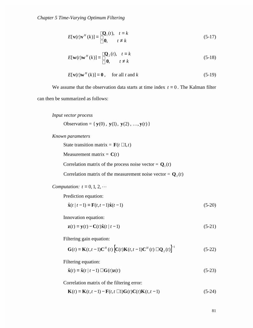
Chapter 5 Time-Varying Optimum Filtering
81
≠=
=kt
kttktE H
,
),()]()([ 1
0
Qvv (5-17)
≠=
=kt
kttktE H
,
),()]()([ 2
0
Qww (5-18)
0wv =)]()([ ktE H , for all t and k (5-19)
We assume that the observation data starts at time index 0=t . The Kalman filter
can then be summarized as follows:
Input vector process
Observation = { )0(y , )1(y , )2(y , …, )(ty }
Known parameters
State transition matrix = ),1( tt +F
Measurement matrix = )(tC
Correlation matrix of the process noise vector = )(1 tQ
Correlation matrix of the measurement noise vector = )(2 tQ
Computation: �,2,1,0=t
Prediction equation:
)1(ˆ)1,()1|(ˆ −−=− ttttt xFx (5-20)
Innovation equation:
)1|(ˆ)()()( −−= ttttt xCyz (5-21)
Filtering gain equation:
[ ] 1
2 )()()1,()()()1,()(−+−−= ttttttttt HH QCKCCKG (5-22)
Filtering equation:
)()()1|(ˆ)(ˆ ttttt zGxx +−= (5-23)
Correlation matrix of the filtering error:
)1,()()()1,()1,()( −+−−= ttttttttt KCGFKK (5-24)

Chapter 5 Time-Varying Optimum Filtering
82
Correlation matrix of the prediction error:
)(),1()(),1(),1( 1 tttttttt H QFKFK +++=+ (5-25)
where 1),1()1,( −+=+ tttt FF
Initial conditions:
)]0([)1(ˆ xx E=−
])])0([)0(()])0([)0([()1( HEEE xxxxK −⋅−=−
The Kalman filter summarized above is for estimating the state vector )(tx . In the
time-varying filter problem we consider, the filtering is for estimating the desired signal
)(td , embedded in the observed data )()()( twtdty += - here we assumed scalar (single-
channel) output. The estimate of the desired signal can be obtained from the state vector
estimate according to
)(ˆ)()(ˆ tttd xC= (5-26)
5.4 Summary and Discussion
We reviewed the Wiener filter and the Kalman filter with the time-varying
filtering problem in mind. The main obstacle in applying these optimum filters is the lack
of information. As pointed out earlier, in many application scenarios, we have only
observation data and do not have known state equations, time-dependent correlation
functions, or power spectra. To solve this problem, in the next chapter, we will develop
TVAR model based Kalman and Wiener filters.
Chapter 6 Time-Varying Optimum Filtering Based on TVAR Modeling
83
Chapter 6
TIME-VARYING OPTIMUM FILTERING BASED
ON TVAR MODELING
In this chapter, we develop the TVAR model based Kalman filter and TVAR
model based Wiener filter. Their performance are compared using both known TVAR
parameters and estimated TVAR parameters. The results show that the TVAR based
causal Wiener filter is a nearly-optimal causal filter.
6.1 Introduction
In Chapter 3 we studied time-varying notch filtering using the TVAR based IF
estimator for interference rejection in DSSS communications. Those “brute force” time-
varying notch filters are controlled only by instantaneous frequency (IF) estimates, rather
than formed according to some optimality criterion . In this chapter, we develop optimum
time-varying filtering based on the TVAR model, including the TVAR based Kalman
filter (TVAR-KF) and TVAR based Wiener filters (TVAR-WF). We model the observed
data with a TVAR model, and use the general Kalman filter and Wiener filter, as
presented in Chapter 5, to form filters using TVAR parameters.

Chapter 6 Time-Varying Optimum Filtering Based on TVAR Modeling
84
We aim at optimal or nearly optimal recovery of a desired signal from a data
record. The signal may be highly non-stationary, the additive contaminating noise may
also be non-stationary, and the signal and noise may overlap in both time and frequency.
From Chapter 5, we know that the optimum filter exists for such cases. The problem in
implementing the optimum filter is the lack of required knowledge, such as the time-
dependent correlation functions needed to solve for the Wiener filter in the time-domain.
In this chapter, we assume that the knowledge required to form the optimum
filters given in Chapter 5 is not available. Instead, we assume that the observed data fits a
TVAR model. Such data are widely found in engineering, such as speech signals and
frequency modulated (FM) signals in noise. Based on this assumption, we can estimate
the TVAR parameters from the data, and then use the parameter estimates to form an
optimum or nearly-optimum filter.
The TVAR-KF is developed by setting up the state-space representation of the
TVAR model. If the observed data is indeed generated from such a TVAR system, that is,
there is no modeling error, and the exact TVAR parameters are used, which means they
are free of estimation error, then the TVAR-KF is the optimal causal filter since it
corresponds directly to the general KF. We also propose a time-varying Wiener filtering
method based on TVAR modeling. By approximating the time-varying nature of the
parameters with combinations of some known functions of time, the proposed TVAR
based Wiener filter is able to handle rapidly varying processes. Both the ideal non-causal
TVAR-WF and the causal TVAR-WF are formulated based on the TVAR model.

Chapter 6 Time-Varying Optimum Filtering Based on TVAR Modeling
85
6.2 TVAR Kalman Filter
6.2.1 Method
Consider an observation )(ty , consisting of desired signal )(td and additive noise
)(tw , which is assumed to be uncorrelated with the signal )(td :
)()()( twtdty += (6-1)
We model the signal with a TVAR model, which is given by (1-1) and rewritten here as
)()()()(1
teitdtatdp
ii +−−= ∑
=
(6-2)
Now we want to find the state-space description equivalent of the TVAR model in
(6-2). The state-space equations (5-15)-(5-16) are rewritten here as
)()(),1()1( ttttt edFd ++=+ (6-3)
)()()()( tttt wdCy += (6-4)
It is straightforward to verify that a state-space description of the TVAR model is
Tptdtdtdt )](,),2(),1([)( −−−= �d , ( 1×p ) (6-5)
Ttet ]0,,0,0),([)( �=e , ( 1×p ) (6-6)
)]([)( tyt =y , ( 11× ) (6-7)
)],([)( twt =w ( 11× ) (6-8)
−−−−
=+
−
0100
0010
0001
)()()()(
),1(
121
���
�
� tatatata
tt
pp
F , ( pp× ) (6-9)
)]()()([)( 21 tatatat p−−−= �C , ( p×1 ) (6-10)

Chapter 6 Time-Varying Optimum Filtering Based on TVAR Modeling
86
With TVAR parameters, Kalman filtering can be performed based on the state-
space description of the TVAR model. We call this method the TVAR based Kalman
filter (TVAR-KF).
6.2.2 Example
As an example of the application of the TVAR-KF, we apply the filter to a fast-
varying signal in white Gaussian noise. A real-valued 200-sample data record starts as
low-pass at 0=t and ends as high-pass at 199=t . The data is generated as a fourth-
order TVAR process plus white Gaussian noise at SNR = 0dB. The two complex-
conjugate pole pairs coincide, and rotate in the z-plane over time according to
199,,1,0,)2008
305.0(2exp5.0)()( 4,32,1 �=
+±== t
tjtptp π
The trajectories of the poles and the corresponding TVAR coefficients 4,1,0),( �=itai ,
as functions of time, are shown in Figure 6-1.
The excitation process to the TVAR model is a zero-mean, unit-variance, white
Gaussian process. The waveforms of a realization of the resulting TVAR process, which
is the desired signal, and the noisy data are plotted together in Figure 6-2. Observe that
the desired signal varies from low-pass to high-pass and wanes in the middle as the poles
are getting farther apart when they meet the imaginary axis. Also note that the additive
noise is stationary over the data record and dominates the observations in the middle of
the data record.

Chapter 6 Time-Varying Optimum Filtering Based on TVAR Modeling
87
( a ) ( b )
Figure 6-1. A fast-varying fourth-order TVAR process that starts as low-pass and ends as high-pass: (a) pole trajectories in z-plane: (b) TVARcoefficients as functions of time.
Figure 6-2. Waveforms of the data record and the desired signal, SNR=0dB.
Using the known TVAR parameters, that were used to generate the data, to form a
TVAR-KF, boosts SNR from 0dB to 4.24dB, which is evaluated as the ratio of energies
in the entire data record for the desired signal and the output error. The known TVAR-KF
output is plotted in Figure 6-3 (a) against the desired signal.

Chapter 6 Time-Varying Optimum Filtering Based on TVAR Modeling
88
Next we use the TVAR parameters estimated from the data record to form an
estimated TVAR-KF. The resulting filtered output is compared with the desired signal in
Figure 6-3 (b). The filter improves SNR from 0dB to 3.75dB, which is successful even
though it produces about 0.5 dB less improvement than was obtained from using the
exact parameters.
( a )
( b )
Figure 6-3. Output of TVAR-KF compared with desired signal:( a ) using known TVAR parameters, SNR=4.238dB,( b ) using estimated TVAR parameters, SNR=3.754dB.

Chapter 6 Time-Varying Optimum Filtering Based on TVAR Modeling
89
6.3 TVAR Wiener Filter
In this section, we develop the TVAR model based Wiener filter, in both causal
and non-causal versions, and then present an example in details. The performance of the
proposed TVAR Wiener filter and the TVAR Kalman filter developed in Section 6.2 will
be studied further through simulations in Section 6.4.
6.3.1 Method
Consider an observation )(tx , consisting of desired signal )(td and additive noise
)(tw :
)()()( twtdtx += (6-11)
Assuming that the noise )(tw is uncorrelated with the signal )(td , implies that the cross-
spectrum between them is zero, i.e. 0)( =zPwd . Consequently, the cross-spectrum
between the data and the desired signal is
)()()()( zPzPzPzP dwdddxd =+= (6-12)
and, similarly, the power spectrum of the data is
)()()( zPzPzP wdx += (6-13)
Recall from Chapter 5 that minimizing the mean squared error (MSE) of estimating )(td
from )(tx leads to the Wiener filter [37]. Using (6-12) and (6-13), the IIR WF in the
frequency domain is then expressed as
)()(
)(
)(
)()(
zPzP
zP
zP
zPzH
wd
d
x
xd
+== (6-14)

Chapter 6 Time-Varying Optimum Filtering Based on TVAR Modeling
90
which is the power spectrum ratio of the desired signal to the observed signal. This is the
stationary Wiener filter, where second-order wide-sense stationarity was assumed in the
derivation.
For time-varying cases, an optimal filter should be a time-varying system that
minimizes the mean squared estimation error. When the time-varying nature is assumed
to be relatively slow, adaptive algorithms [38] have been well established. Our interest is
in those cases where the parameters of the desired signal and/or the observation noise
varies so rapidly that adaptive filtering algorithms are not appropriate, and/or those cases
where training data is not available.
For a non-stationary process, we form a time-varying filter ),( ztH by
concatenating the optimal filters at each time moment t, which can be expressed as
),(),(
),(
),(
),(),(
ztPztP
ztP
ztP
ztPztH
wd
d
x
xd
+== (6-15)
where ),( ztPd , ),( ztPw and ),( ztPx are the time-dependent spectra or time-frequency
power distributions. This time-varying filter is essentially the same as the time-frequency
design of non-stationary Wiener filters theoretically derived via WVD and WS (Weyl
Symbol) by Kirchauer, Hlawatsch, and Kozek [21], as mentioned in Chapter 1. We
advocate the use of the TVAR model in the design of time-varying filters for the same
reason that parametric methods are widely used for various problems in stationary cases,
and also for the reason that we can form the causal Wiener filter by TVAR spectral
factorization. Compared to the WVD, other attractive features of TVAR spectra include
high spectral resolution, being cross-term free, and providing the ability to handle short
data blocks.

Chapter 6 Time-Varying Optimum Filtering Based on TVAR Modeling
91
The filter expressed in (6-15) is non-causal. Similar to the stationary case [37],
based on the spectral factorization
)1,(),()(),( ∗∗= ztCztCtKztPx (6-16)
yields the corresponding causal filter:
+∗∗
=
)1,(
),(
),()(
1),(
ztC
ztP
ztCtKztH d
c (6-17)
where ),( ztC , a rational form with monic numerator and denominator polynomials and
all poles and zeros located inside the unit circle, represents the causal minimum-phase
factor of ),( ztPx , and the notation +][ refers to the causal part of the inverse Z-
transform.
If both signal and noise are modeled by a TVAR model, with TVAR coefficients
denoted as di ptta �,1,0),( = , for the signal )(td and wi pttb �,1,0),( = , for the noise
)(tw , their respective TVAR based time-dependent power spectra are:
)1,(),(),(
2
∗∗=ztAztA
ztP dd
σ(6-18a)
)1,(),(),(
2
∗∗=ztBztB
ztP ww
σ(6-18b)
where 2dσ and 2
wσ are the variances of the white excitation processes generating )(td
and )(tw , respectively, and the polynomials are defined as follows
ip
ii ztaztA
d −
=∑= )(),(
0, 10 ≡a (6-19a)
ip
ii ztbztB
w −
=∑= )(),(
0, 10 ≡b (6-19b)

Chapter 6 Time-Varying Optimum Filtering Based on TVAR Modeling
92
The TVAR power spectrum expression in (6-18) is a direct extension of the AR
spectrum in the stationary case [30]. We also have shown that this expression can be
derived from Priestley's evolutionary spectrum (ES) theory as a special case of the ES. A
brief description of Priestley’s evolutionary spectrum theory, its relation to this research,
and how the ES leads to the TVAR spectrum in (6-18) is given at the end of this
document as Appendix B.
Let ),( ztD be the monic numerator polynomial of ),( ztC , i.e.
),(),(
),(),(
ztBztA
ztDztC = (6-20)
Consequently, the ideal non-causal TVWF in (6-15) can now be expressed as
=
∗∗
∗∗
)1,()(
)1,(
),()(
),(),(
ztDtK
ztB
ztDtK
ztBztH nc (6-21)
Note two distinct factors in (6-21): the causal part in the first brackets, and the
corresponding anti-causal part in the second brackets. Similarly, the causal TVWF in (6-
17) is specified as
+∗∗
∗∗
=
)1,(),(
)1,(
),()(
),(),(),(
ztDztA
ztB
ztDtK
ztBztAztH c (6-22)
In many application cases, the additive measurement noise )(tw in (6-13) can be
treated as being white noise, such as receiver thermal noise in communications. In such
cases 2),( ww ztP σ= and 1)1,(),( ≡≡ ∗∗ ztBztB , so that the filters in (6-21) and (6-22)
are simplified accordingly.
The non-causal filter in (6-21) can be realized based on data blocks in two steps,
similar to the MPSE based non-causal time-varying Wiener filter by Beex and Xie [22].

Chapter 6 Time-Varying Optimum Filtering Based on TVAR Modeling
93
First the data block is filtered by the causal part, corresponding to the first bracketed term
in (6-21), and then the anti-causal part is implemented by filtering the temporal output
from the first step backward with the causal part of the transfer function.
In practice, with a priori information about the signal and the noise, ),( ztA and
),( ztB may be identified from the observations. Since the filter coefficients are directly
related to the TVAR coefficients, the parameter estimation, filter coefficient calculation,
and filtering operation can be implemented in a block-by-block fashion.
6.3.2 Example
We illustrate the performance of the proposed TVAR based IIR TVWFs through
an example. The time-varying filters were implemented in the Direct Form I, with the
coefficients updated for each sample. The implementation of the non-causal version is
based on the entire data block filtered in the forward-then-backward way.
We use the same data as was used in the example for the TVAR-KF in Subsection
6.22, with the time-variation laws shown in Figure 6-1 and waveforms in Figure 6-2.
First, we assume that the exact information on the TVAR parameters, used to generate
the data, is known. Both the causal and non-causal versions of the TVAR-WF are formed
using the exact TVAR parameters. Next we use the TVAR parameters estimated from the
given data record to form the non-causal and causal TVAR-WFs.
In Figure 6-4, the magnitude responses of the non-causal TVAR-WFs using both
the exact and the estimated TVAR parameters are shown in terms of gain contours (in
decibels) on the time-frequency plane. These filters track the trajectory of the signal poles

Chapter 6 Time-Varying Optimum Filtering Based on TVAR Modeling
94
shown in Figure 6-1: they both start as a low-pass response, vary to a band-pass, and end
as a high-pass, even though their magnitude gain contours look different.
( a ) ( b )
Figure 6-4. The magnitude response (dB) contour plots of the ideal non-causal TVAR-WF:( a ) using the known TVAR parameters,( b ) using TVAR parameters estimated from the data record.
Applying the above filters to the data record, boosts the SNR from 0dB to
5.385dB and 4.249dB by using the known and estimated parameters respectively. The
output waveforms are compared with the desired signal in Figure 6-5. Compared to the
outputs of the TVAR-KF in Figure 6-2, for the same data and parameters, the non-causal
TVAR-WF yields significantly higher filtering gains; about 1dB higher when using the
known parameters and about 0.5dB higher when using estimated parameters. An
explanation for the latter is that the TVAR-KF is causal while the ideal TVAR-WF is
non-causal and hence may have much better performance.

Chapter 6 Time-Varying Optimum Filtering Based on TVAR Modeling
95
( a )
( b )
Figure 6-5. Output of the non-causal TVAR-WF compared with desired signal:( a ) using known TVAR parameters, SNR=5.385dB,( b ) using estimated TVAR parameters, SNR=4.249dB.
Now we examine the causal TVAR-WF. Similarly, the time-varying magnitude
responses of the causal TVAR-WF are shown in Figure 6-6. Again, they start as a low-
pass filter, become band-pass in the middle, and end as a high-pass filter. The output
waveforms are shown in Figure 6-7. Using the known parameters, the causal TVAR-WF
yields an SNR improvement of 4.204dB, which is very close to the 4.238dB provided by
the (causal) TVAR-KF that uses the same information. Using the estimated parameters,

Chapter 6 Time-Varying Optimum Filtering Based on TVAR Modeling
96
the causal TVAR-WF yields output SNR of 3.745dB, which is also very close to the
output SNR of 3.754dB produced by the corresponding Kalman filter. This confirms that
the proposed TVAR-WF is nearly optimal. We will further examine this issue through
simulations in the next section.
( a ) ( b )
Figure 6-6. The magnitude response (dB) contour plots of the idealcausal TVAR-WF:( a ) using the known TVAR parameters,( b ) using the TVAR parameters estimated from the data record.

Chapter 6 Time-Varying Optimum Filtering Based on TVAR Modeling
97
( a )
( b )
Figure 6-7. Output of causal TVAR-WF compared with desired signal:( a ) using known TVAR parameters, SNR=4.204dB,( b ) using estimated TVAR parameters, SNR=3.745dB.
6.4 Simulation Results for TVAR based Optimum Filters
We have developed the TVAR based optimum filters, including the TVAR-KF
and the TVAR-WF, in both non-causal and causal versions. We also illustrated their SNR
improvement capacity through an example. In this section, we further examine their
performance through simulations. The results confirm that the proposed causal TVAR-

Chapter 6 Time-Varying Optimum Filtering Based on TVAR Modeling
98
WF performs nearly as well as the Kalman filter that uses the same information, i.e., the
TVAR-KF, implying that the causal TVAR-WF is a nearly-optimum causal filter.
In the simulations, the same pole trajectories and TVAR parameters are used as
were used for the example in the preceding section, as shown in Figure 6-1. For each
simulation trial, different realizations of both signal and noise are generated. The trials
are repeated for various input SNR values. Figure 6-8 shows average filtering gain versus
input SNR for different filters. The causal TVAR-WF performs almost identically as the
TVAR-KF. As expected, the non-causal WF outperforms the causal filters significantly,
for both cases, i.e. using known or estimated parameters. This is a major advantage for
the non-causal filter. In some applications, causality is not too serious a concern when a
limited processing delay is acceptable, such as in a communication system. In such
scenarios, the non-causal TVAR-WF can be used.
( a ) ( b )
Figure 6-8. Average SNR gain at various input SNR for the TVAR based filters:( a ) using known TVAR parameters,( b ) using estimated TVAR parameters.

Chapter 6 Time-Varying Optimum Filtering Based on TVAR Modeling
99
We also observe the performance variation among different filters for the same
data record and among different data realizations with the same statistical properties.
Figure 6-10 shows output SNR values for different filters for each individual data record
and their distributions among 25 trials at various input SNR levels. First, it is shown that
the causal TVAR-WF performs consistently close to the optimal TVAR-KF for each
given data record. This further confirms that the TVAR-WF is nearly-optimal. Second,
parameter estimation error noticeably decreases the performance of these TVAR based
filters. This means that the best performance that can be achieved in practice may be far
below the theoretically potential optimum performance. Third, the performance varies
significantly from data to data. Finally, nevertheless, the proposed TVAR based optimum
filters, either using known or estimated parameters, always improve the SNR for a data
block.
In the experiment, a wide band signal is used, with also wide instantaneous
bandwidth (poles far inside the unit circle), in white (wideband) noise. This represents a
tough case for the task of filtering. In such cases, a joint time-frequency cut-off filter is
not appropriate, not to mention the conventional frequency-domain filter, and,
consequently, an optimal or sub-optimal time-varying filter is necessary. For the cases of
a signal with narrow instantaneous bandwidth in wideband noise, or vice versa, the
filtering gain can be much higher (in terms of dB value) than shown in these examples,
which is in the range of several decibels. The latter scenario will be shown in the next
chapter, where the idea of the TVAR-WF is applied to FM interference rejection for
DSSS communications. As seen in Chapter 4, in the latter problem we have a wideband
communication signal and an interference with narrow instantaneous bandwidth.

Chapter 6 Time-Varying Optimum Filtering Based on TVAR Modeling
100
( a )
( b )
( c )
Figure 6-9. Output SNRs for different filters at each data record and theirdistribution among 25 trials,Labels to denote types of filter:
Nonc, Kalm, Caus = Non-causal TVAR-WF, TVAR-KF, CausalTVAR-WF, using known TVAR parameters,
Nonc^, Kalm^, Caus^ = Non-causal TVAR-WF, TVAR-KF, CausalTVAR-WF, using estimated parameters,
Input SNR: ( a ) 0dB, ( b ) 3dB, ( c ) 6dB.

Chapter 6 Time-Varying Optimum Filtering Based on TVAR Modeling
101
6.5 Summary
In this chapter we developed TVAR based optimum filters, including the TVAR
based Kalman filter and causal and non-causal Wiener filters. By modeling the data
record with the TVAR model, the TVAR based filters were developed from the basic
optimum filters presented in Chapter 5. We showed that the TVAR based time-varying
extension of the stationary Wiener filter solution provided nearly optimal performance.
Using TVAR parameters estimated from the data record yields significant filtering gain
on average. However, individual realizations, while still producing non-negative filtering
gain, can produce performance noticeably below the theoretically optimum gain due to
parameter estimation errors.
Chapter 7 Soft-Cancellation of FM Interference Based On Optimal Filtering
102
Chapter 7
SOFT-CANCELLATION OF FM INTERFERENCE
BASED ON OPTIMAL FILTERING
As an application of the TVAR based Wiener filter presented in Chapter 6, in this
chapter, we develop a time-varying filter formulation for "soft-cancellation" of FM
interference in DSSS communications. This filter uses full spectral information of the
received data and is aimed at minimum signal distortion. Part of the results in this chapter
were published earlier [67].
7.1 Introduction
Recently, time-frequency distributions (TFD) have been applied to suppress
rapidly varying nonstationary interference in direct sequence spread spectrum (DSSS)
communications [47-50,58]. Amin and his colleagues [47,48,60] studied interference
excision using a time-varying notch filter with the null placed at the instantaneous
frequency (IF) of the interference, where the IF was estimated from Wigner-Ville
distributions (WVD). Other than invoking TFD's, in Chapter 4 we suggested using
TVAR based IF estimation in the notch filter method to improve the IF estimation and

Chapter 7 Soft-Cancellation of FM Interference Based On Optimal Filtering
103
hence the system performance, especially for those practical situations where the
frequency modulation can not be assumed to follow a linear law.
The FIR notch filter based interference suppression methods [48,57] are simple to
implement once an IF estimate has been determined. However, this method suffers from
a major limitation. That is, it uses only the IF information of the interference. The notch
filter is formed regardless of the relative strength , instantaneous bandwidth, or other
spectral characteristics of the interference. Such a notch filter significantly improves
system performance for a strong mono-component tonal or FM interference by cutting
the interference at the IF very deeply. However, when the interference becomes weak or
absent, the brute force filter may significantly deteriorate system performance since it
also distorts the signal. A threshold is thus needed to switch the notch filter on or off
based on the received data energy or power [48]. To deal with this problem, Wang and
Amin [66, 70] also suggested placing the filter zeros inside the unit circle with their
radius determined by the relative interference power.
In this chapter, we attack these problems by exploiting the full spectral
information about the interference, which is made possible with the TVAR model. Since
the filter is not aimed at annihilating as much of the interference component as possible,
we refer to our strategy as soft-cancellation. As earlier in Chapter 4, we model the
received signal with a time-varying autoregressive model. However, here, instead of
estimating the IF using the model, we use the model parameters to directly form a filter.
We apply the time-varying Wiener filter that was developed in Chapter 6 to solve this
problem. The TVAR-WF is tailored (as a result of its mean squared error criterion) to the
received data with minimum signal distortion as the objective. In Chapter 6, we

Chapter 7 Soft-Cancellation of FM Interference Based On Optimal Filtering
104
developed the TVAR based optimum filters including the ideal non-causal TVAR-WF,
the causal TVAR-WF, and the TVAR-KF. Among these, the non-causal TVAR-WF
yields the best performance and the associated limited processing delay is tolerable in a
communication system. Therefore, we will develop the interference rejecting filter based
on the non-causal TVAR-WF.
7.2 A General Description of Interference Suppression Based on TVAR
Modeling
In Figure 7-1, we give the system diagram of a DSSS receiver with interference
suppression using time-varying filtering based on TVAR modeling. The TVAR
parameters are identified from the received data and are used to form the time-varying
filter. The filtering operation is performed before de-spreading in baseband. This method
differs from the brute force notch filtering method, which may use a TVAR based IF
estimate as studied in Chapter 4, in two respects. First, the filter ),( ztH is formed
directly from the TVAR parameters, without involving IF estimation. Second, the full
spectral information carried by the set of TVAR parameters is used to form the
cancellation filter. The objective that will be used here to form the filter ),( ztH is
minimum signal distortion, as presented in this chapter. Another objective, whiteness of
the filter output, will be presented in Chapter 8. Just as in the diagram of the notch filter
based method (Figure 4-1), BPSK modulation and code-on-pulse spreading are assumed
in Figure 7-1.

Chapter 7 Soft-Cancellation of FM Interference Based On Optimal Filtering
105
Down-convert
tobaseband
Sampler
FM interferenceDSSS signal
RFfront-end
thermalnoise
TVARParameterEstimation
filterH (t,z)
r(t) y(t)
Despreadingsequence
Sum overeach bitinterval
Bitdecision
PN code
Interferencesuppression
BPSK DSSS demodulator
Databuffer
Figure 7-1. Block diagram of the DSSS receiver with TVAR basedinterference suppression.
7.3 FM Interference Suppression Based on TVAR-WF: Method and
Example
We propose a time-varying interference suppression filter formulation that tailors
the filter to fit the full time-varying spectral information about both the interference and
the desired signal. Our formulation is aimed at minimizing the mean squared error of the
output waveform. The TVAR model is used to identify the time-varying interference and
to accordingly form the interference suppression filter based on the time-varying Wiener
filter.
7.3.1 Method
At the receiver of a DSSS communications system, an interference suppression
filter is applied before demodulation. We consider a received signal )(tr , where t refers
to discrete time, composed of the DSSS signal )(ts , noise )(tw and interference )(ti :
)()()()( titwtstr ++= (7-1)

Chapter 7 Soft-Cancellation of FM Interference Based On Optimal Filtering
106
Here the noise )(tw is assumed stationary and white. The DSSS signal )(ts is also
assumed stationary and white (non-Gaussian). In practice the DSSS signal may be
“slightly colored”, depending on the sampling rate (samples per chip) and the specific PN
sequence used. The interference )(ti could be from a broad range of time-varying
sequences, such as a hostile jammer or an FM communication signal (for example, a
cellular system overlapping CDMA and AMPS). The three components are assumed
independent.
We feed )(tr to a time-varying filter ),( ztH to suppress )(tw , and denote the
output as )(ty . The filter is aimed at minimizing the mean squared error
}|{| 2)()()(Emin tytwts −+ (7-2)
This is a mean square estimation problem [19] with )(ts + )(tw treated as the desired
signal. For stationary processes, solving (7-2) leads to the Wiener filter [37]:
H zP z P z
P z P z P zstationarys w
s w i( )
( ) ( )
( ) ( ) ( )=
++ +
(7-3)
whereP z∗ ( ) is the power spectral density function of the process denoted by the
subscript. As in Chapter 3, to extend this Wiener filter to time-varying cases, we
concatenate the optimal filters at each time instant t , and thus form the time-varying
filter:
),()()(
)()(),(
ztPzPzP
zPzPztH
iws
ws
+++
= (7-4)
where ),( ztPi is the time-varying spectrum of the interference.

Chapter 7 Soft-Cancellation of FM Interference Based On Optimal Filtering
107
Let )(ts and )(tw , both white, have spectra σs2 and σw
2 respectively. Let
2dσ =σs
2 +σw2 = P z P zs w( ) ( )+ , so that the time-varying filter in (7-4) becomes
),(),(
2
2
ztPztH
id
d
+σσ
= =2),(1
1
di ztP σ+(7-5)
This is an IIR filter aimed to best recover the waveform in least mean square sense. The
transfer function of this filter approximates unity at the frequencies where the
interference spectrum is much weaker than the signal plus noise. Thus, unlike the time-
varying notch filtering method, which distorts the signal and hence deteriorates system
performance when the interference is absent or weak, this filter keeps the received signal
intact if the interference is absent. The filter in (7-5) suppresses the interference
according to its time-varying spectrum. It also applies to more complicated interference
types, i.e. those which exhibit significant instantaneous bandwidth, as long as the
received signal can be well approximated by a TVAR model.
To implement filter (7-5), we need to estimate ),( ztPi , the time-varying power
spectrum, or time-frequency distribution, of the interference. It is well known that a
stationary narrow-band signal in white noise fits an ARMA model, and in case of
moderate to high SNR, it can be approximated with an AR model. Extending to the time-
varying cases, we approximately model the time-varying interference with a TVAR
model.
As mentioned in Chapter 6, if we model the interference using the TVAR model,
the power spectrum is expressed as:
)1,(),(),(
2
∗∗σ
=ztAztA
ztP ii (7-6)

Chapter 7 Soft-Cancellation of FM Interference Based On Optimal Filtering
108
where ip
ii ztaztA −
=∑= )(),(
0
with { )(tai } being TVAR coefficients ( 1)(0 ≡ta ), and “*”
denoting the complex conjugate operation. Substituting (7-6) in (7-5), the interference
suppression filter is expressed as
22)1,(),(
)1,(),(),(
diztAztA
ztAztAztH
σσ+= ∗∗
∗∗
(7-7)
At each time instant t, we factor the denominator polynomial as follows
)1,(),()()1,(),( 22 ∗∗∗∗ =σσ+ ztDztDtKztAztA di (7-8)
where ),( ztD is in the form of ip
ii ztdztD −
=∑= )(),(
0
, with 10 ≡d , and has all its roots
inside the unit circle. The filter becomes
⋅
⋅= ∗∗
∗∗
)1,(
)1,(
),(
),(
)(
1),(
ztD
ztA
ztD
ztA
tKztH (7-9)
The first set of brackets encloses the causal minimum-phase factor of the transfer
function, and the second set of brackets encloses the anti-causal maximum-phase factor.
The overall filter is zero-phase and non-causal. It can be realized with delay by first
filtering a block of input forward with the causal part transfer function and then realizing
the anti-causal part by filtering the previous result backward, as shown in Figure 7-2. The
delay due to the non-causality is related to the processing power and the data block size.
The data block size is likely on the order of hundreds of samples, and therefore on the
order of a symbol or bit interval considering a few samples per chip and the number of
chips per symbol commonly used. This delay is insignificant compared to the delay
introduced by some other algorithms commonly used in a communication system, such as
block coding, interleaving/scrambling, or Viterbi decoding.

Chapter 7 Soft-Cancellation of FM Interference Based On Optimal Filtering
109
Flipdata
block
⋅
),(
),(
)(
1
ztD
ztA
tK
),(
),(
ztD
ztA Flipdata
block
Figure 7-2. Implementation of the non-causal filter by filtering forward andthen backward.
Half of the filter,
),(
),(
ztD
ztA, is an IIR filter with zeros and poles guaranteed to fall
inside the unit circle. It has p zeros and poles, where p is the autoregressive order. For
interference at different power levels (different SIR levels), the zeros are always located
at the interference frequencies, while the locations of the poles vary. At high SIR, the
poles are close to the zeros, and therefore the magnitude response tends to be flat. At low
SIR, the poles are far away from the zeros, and therefore deep notches are formed to
reject the interference.
In the forward-and-backward implementation, a filter transient appears at both
ends of the data block. Proper block overlapping can be introduced to cover most of the
transient at both ends of the data block. This makes the size of the data block slightly
larger.
7.3.2 Example
To illustrate how the proposed interference rejection filter is tailored to the
received data, we plot the frequency response of an example of this filter in Figure 7-3,
and compare it against the brute-force FIR notch filter (see Section 4.3.1 for details of the
length-5 FIR notch filter). Here an FM interference with a constant frequency is

Chapter 7 Soft-Cancellation of FM Interference Based On Optimal Filtering
110
considered, and the exact frequency and autoregressive model parameters are assumed
known and used in forming the filter in each case. The frequency response shown could
be viewed as an "instantaneous frequency response" for the time-varying filter in a time-
varying case. In Figure 7-3, we see that the proposed filter is close to the brute-force
notch filter when the interference is very strong, i.e., at very low SIR. On the other hand,
it approximates a flat unity response when the SIR is very high, where interference
rejection is not needed.
7.4 Simulations of Interference Suppression Based on TVAR-WF
The effectiveness of the proposed interference suppression filter is illustrated by
comparing it with notch filter based brute-force cancellation. Consider a single-user
DSSS system with BPSK modulation and processing gain N=15 chips per bit. The
spreading code is a randomly generated binary PN sequence. The noise in the received
signal is an additive white Gaussian noise. It is assumed that the channel is free of fading
and ISI (inter-symbol interference). The standard correlation de-spreading receiver is
used, with or without an interference suppression filter. Without interference, the BER
(bit error rate) of the system would be solely determined by SNR according to
)2( 0NEQP be = . Here bE stands for the signal bit energy, 0N is the one-sided noise
power spectral density, and )(⋅Q is the standard Q function, defined as
λλπ
dzQz
)2exp(2
1)( 2∫
∞−= .

Chapter 7 Soft-Cancellation of FM Interference Based On Optimal Filtering
111
Figure 7-3. Magnitude responses of the proposed TVAR-WF filter (solid)vs. the brute force FIR notch filter (dashed), at SIR = −60dB (top left),−30dB, −10dB, 0dB, 10dB, and 30dB (bottom right).

Chapter 7 Soft-Cancellation of FM Interference Based On Optimal Filtering
112
7.4.1 Case 1: Fixed-Frequency and Known Parameters
Before looking at a more realistic case, we first examine the performance of the
proposed TVAR based time-varying Wiener filter for a simple, yet important case. Here
we consider an interference with fixed frequency over the data block in order to examine
the advantage of the Wiener filter over the brute-force notch filter, without involving the
time-varying characteristics of both kinds of filters.
In Figure 7-4, the proposed WF based interference suppression is compared with
interference suppression using the length-5 FIR notch filter in terms of BER versus
signal-to-interference ratio (SIR) for 0NEb = 8dB. At each simulation trial, a new
interference frequency is generated randomly, evenly distributed between 0 and 0.5Hz
(normalized to unity sampling rate). Thus, the figure reflects the average performance of
the filters at a random frequency. Here chip-rate sampling is used, i.e., 1 sample per chip.
The exact frequency and model parameter information is used for both the proposed filter
and the notch filter. For comparison, the simulated BER for the plain receiver without
interference suppression ("no filtering") and the BER evaluated from the Q function for
the interference-free case ("limit by SNR") are also shown in the figure.
For this case of fixed frequency with known parameters, the proposed Wiener
filter outperforms the brute-force FIR notch filter for the entire range of SIR, and is
especially advantageous when the SIR is not extremely low. The flatness of the BER
versus SIR curve for the notch filter reflects the fact that the notch filter distorts the signal
while deeply canceling the interference. The TVAR-WF yields desirable performance

Chapter 7 Soft-Cancellation of FM Interference Based On Optimal Filtering
113
over the entire range of SIR while the brute-force notch filter harms the system when the
interference is weak.
Figure 7-4. Comparing the proposed TVAR-WF with the FIR notch filterin terms of BER versus SIR for the DSSS scenario with fixed frequencyand known parameters, 0NEb = 8dB.
7.4.2 Case 2: Nonlinear FM Jammer Using Estimated Parameters
Now we examine a more practical case where the TVAR parameters are estimated
from a block of data involving a nonlinear FM jammer. As in the examples in Chapter 4,
a DSSS system using BPSK modulation and processing gain of 15 chips per bit is
considered. The sampling rate is 8 samples per chip, or equivalently, 120 samples per bit.
The data block is of length 136 samples. The 120 samples in the middle of the data block
represent a bit, while the first 8 samples and the last 8 samples of the data block are part
of the bits before and after. The bit decision is made based on each data block. The extra
samples near the ends of the data block are included to pass the transients of the

Chapter 7 Soft-Cancellation of FM Interference Based On Optimal Filtering
114
backward-then-forward non-causal filter implementation shown in Figure 7-2. In this
case, a nonlinear FM jammer is considered, with instantaneous frequency as shown in
Figure 7-5, which is generated by the IF law
135,,1,0),1272
sin(3.015.0)( �=⋅π+= tt
tf (7-10)
In each simulation trial, the FM jammer is generated independently with a random initial
phase, and a new random binary sequence is generated and used as the spreading code.
Therefore, the simulation result is not dependent on the specific PN code or initial phase.
Figure 7-5. Instantaneous frequency law of the jammer inside the datablock.
The simulated BER versus JSR (jammer-to-signal ratio) with fixed 0NEb =10dB
for the four types of receiver is given in Figure 7-6. The compared receivers include the
plain decorrelating ("no filtering") receiver, the receiver with proposed TVAR-WF based
interference rejection, and the receiver with brute-force length-5 FIR notch filter based
interference rejection in two cases: using the exact (supposedly known) IF or using the

Chapter 7 Soft-Cancellation of FM Interference Based On Optimal Filtering
115
TVAR based IF estimate. We observe that the proposed TVAR-WF method provides the
best performance over the entire range of JSR. This is because the proposed filter, by
using the full spectral information, is capable to “adapt” according to the data, as shown
in Figure 7-3. By contrast, the brute-force notch filtering method provides good
performance improvements when the jammer is strong, but needs to be switched off
when the jammer is not strong, below 10 dB JSR in this case. Even with known
parameters, the notch filter does worse than no filtering at low JSR. We mentioned earlier
in Chapter 3 the existence of an SNR threshold for IF estimation, below which the
performance of IF estimation drops dramatically. This phenomenon materializes here for
the TVAR-IF for JSR below 10dB. Note that estimating IF produces errors relative to the
known IF which cause deterioration of the FIR notch filter approach below 10 dB JSR.
However, estimating TVAR parameters and directly using that information for Wiener
filter design seems to work well even at low JSR. In the latter case there is little
deterioration over not filtering at all. This situation is very desirable, as there is no need
to switch between different methods depending on JSR (which would need to be
measured).

Chapter 7 Soft-Cancellation of FM Interference Based On Optimal Filtering
116
Figure 7-6. BER versus JSR for the proposed TVAR-WF compared withthe notch filter method and the plain receiver without filtering for a case ofnon-linear FM jammer in DSSS, 0NEb = 10dB.
7.5 Summary and Discussion
In the time-varying notch filter based interference cancellation approach, the filter
is formed using the instantaneous frequency of the interference regardless of its power or
other spectral information. Consequently, when the interference is moderate or weak, the
notch filter may cancel more signal than interference, and hence yield deteriorating
system performance. We developed a time-varying filter for interference cancellation in
DSSS communications, which is tailored by the full time-varying spectral information to
minimize the filter output error. The proposed method is a time-varying extension of the
Wiener filter and is based on the TVAR model. The improved performance of the
proposed method was evidenced through simulations.

Chapter 8 TVAR Based Time-Varying Whitening Filter for Soft-Cancellation of FM ...
117
Chapter 8
TVAR BASED TIME-VARYING WHITENING
FILTER FOR SOFT-CANCELLATION OF FM
INTERFERENCE IN DSSS
In this chapter, we propose another time-varying filter formulation for “soft-
cancellation” of interference that uses full spectral information of the received data. The
filter is aimed at flatness of the output spectrum and is referred to as a time-varying
whitening filter. It uses the same information carried in the TVAR parameters as for the
TVAR based Wiener filter studied in Chapters 6 and 7, and is formed as the TVAR
model based time-varying linear prediction error (TVAR-LPE) filter. Since the term
TVAR-WF is reserved for the TVAR based Wiener filter, we refer to the whitening filter
as the TVAR-LPE filter for short.
8.1 Introduction
In the scenario of FM interference rejection in DSSS communications, the
interference has a narrow instantaneous bandwidth, and therefore, has a highly colored

Chapter 8 TVAR Based Time-Varying Whitening Filter for Soft-Cancellation of FM ...
118
time-dependent spectrum. On the other hand, the desired signal has a relatively flat
spectrum. This implies that if a filter is designed to whiten the received data, it must
suppress the interference. We would also like to preserve the signal. This is the basic idea
of interference rejection based on whitening filtering.
Since the spectrum of the FM interference is rapidly time-varying, the whitening
filter should also be rapidly time-varying. The idea of time-varying whitening filtering
based interference rejection is made realizable by TVAR modeling, similar to the cases of
the TVAR-WF and the TVAR-KF. It is well known that in the stationary case the output
of a linear prediction error (LPE) filter associated with an AR model is a white process if
the input is an AR process and the order of the model is high enough, and the LPE filter
output is then referred to as the innovation. The innovation, or LPE, is the component of
the data that can not be represented by the AR model. Similarly, in our time-varying case,
the FM interference can be approximated by a TVAR model with poles close to the unit
circle (it does not have any zeros), while the desired signal, which is wideband and nearly
white, does not fit that model. Therefore, in this scenario, the output of the TVAR based
LPE filter approximates the desired signal.
The TVAR-LPE filter is an FIR filter with as transfer function the inverse of the
transfer function of the TVAR model. The poles of the TVAR model become the zeros of
the TVAR-LPE and those zeros annihilate the interference. For strong interference (high
JSR), the TVAR poles, and consequently the TVAR-LPE zeros, are close to the unit
circle and a deep notch is formed at the angle of each TVAR pole. For weak interference
(low JSR), the estimated TVAR-LPE zeros are away from the unit circle and,

Chapter 8 TVAR Based Time-Varying Whitening Filter for Soft-Cancellation of FM ...
119
consequently, the notch at the angle of each TVAR pole is shallow. In this way, the filter
provides soft-cancellation of the interference, similar to the TVAR-WF based filter.
8.2 FM Interference Suppression Based on TVAR Whitening Filter:
Method and Example
8.2.1 Method
As shown in Figure 7-1, at the receiver of a DSSS communications system, an
interference suppression filter is applied before demodulation. As in Chapter 7, we
consider a received signal )(tr , where t refers to discrete time, composed of the DSSS
signal )(ts , noise )(tw and interference )(ti :
)()()()( titwtstr ++= (8-1)
Here the noise )(tw is assumed stationary and white. The DSSS signal )(ts is also
assumed stationary and white (non-Gaussian). In practice the DSSS signal may be
“slightly colored”, depending on the sampling rate (samples per chip) and the specific PN
sequence used. The interference )(ti could be a hostile FM jammer or an FM
communication signal (for example, a cellular system overlapping CDMA and AMPS).
The three components in (8-1) are assumed to be independent.
We feed )(tr to a time-varying filter ),( ztH to produce a white output. If we
denote the output as )(ty , this means that we want the output )(ty to have a flat time-
dependent spectrum, i.e.
2)1,(),(),( yr ztHztHztP σ=∗∗ (8-2)

Chapter 8 TVAR Based Time-Varying Whitening Filter for Soft-Cancellation of FM ...
120
where 2yσ is the variance of the whitening filter output and ),( ztPr is the time-dependent
power spectrum of the received signal, which was used as the filter input.
As mentioned in Chapter 6, if we model the received signal using the TVAR
model, the power spectrum is expressed as:
)1,(),(),(
2
∗∗=ztAztA
ztPr
σ(8-3)
where 2σ is the variance of the excitation process and ip
ii ztaztA −
=∑= )(),(
0
with { )(tai }
being TVAR coefficients. Substituting (8-3) into (8-2), we have
)1,(),()1,(),(2
2∗∗∗∗ = ztAztAztHztH y
σσ
(8-4)
This suggests that we take
),(),( ztAztH y
σσ
= (8-5)
We can set 22 σσ =y without affecting the output signal to noise ratio and, therefore, the
resulting decision. Then the time-varying whitening filter is simply
),(),( ztAztH = (8-6)
This is also the time-varying linear prediction error (TVAR-LPE) filter.
Compared to the TVAR-WF filter, the TVAR-LPE requires less computational
effort. Once the TVAR parameters are estimated, the TVAR-LPE filter is readily formed,
unlike the TVAR-WF for which polynomial rooting/factorization is needed. Therefore,
the TVAR-LPE method is more practical for cases of multiple-component interference
where a higher autoregressive order is needed for the TVAR model. Another feature of
the TVAR-LPE method is that it is a short FIR filter with the order equal to the order of

Chapter 8 TVAR Based Time-Varying Whitening Filter for Soft-Cancellation of FM ...
121
the TVAR model, which equals the number of interference components (for complex-
valued data and filter) or two times that (for real-valued data and filter).
8.2.2 Example
To illustrate how the TVAR-LPE interference rejection filter is tailored to the
received data, we evaluated a "snapshot" of its time-varying magnitude response and
contrast it in Figure 8-1 against the brute-force notch filter. The frequency responses
shown are instantaneous frequency responses when the IF is at 0.35Hz. It is taken at
59=t in the nonlinear FM jammer case in Section 7.4.2, with the IF described by (7-10)
and shown in Figure 7-5. Here the TVAR-LPE is formed using the TVAR parameters
estimated from a data record while the exact frequency information is used to form the
notch filter. The TVAR-LPE is implemented with TVAR order 1=p and 5=q after
converting the real-valued data to analytic data, with the imaginary part generated via
Hilbert transform filtering.
In Figure 8-1, we see that the magnitude response (in decibels) of the whitening
filter, which is the inverse of the TVAR based spectral estimate of the data, yields a soft
cancellation of the FM interference. That is, when the jammer is weak (lower JSR), the
TVAR-LPE filter adapts to it and the notch becomes shallow or nearly flat when
cancellation is not needed.
At higher interference levels, the TVAR-LPE filter yields an adequate notch
depth, though it is not as deep as for the brute-force notch filter. The advantage of the
TVAR-LPE is its relatively flat response outside the notch area compared to the notch
filter. Consequently, the TVAR-LPE filter results in less signal distortion and could,

Chapter 8 TVAR Based Time-Varying Whitening Filter for Soft-Cancellation of FM ...
122
therefore, even at high JSR, yield lower BER than the brute-force FIR notch filter. At
lower JSR, the frequency response of the TVAR-LPE becomes relatively flat, though not
as flat as for the TVAR based Wiener filter shown in Figure 7-3.
Figure 8-1. A snapshot of magnitude responses of the TVAR-LPE filter(solid) vs. the brute force FIR notch filter (dashed), at JSR = 60dB (top left),30dB, 20dB, and 0dB (bottom right).
We see that the estimated TVAR parameters place the notch precisely at the
interference frequency when the interference is strong. On the other hand, when the

Chapter 8 TVAR Based Time-Varying Whitening Filter for Soft-Cancellation of FM ...
123
interference is weak, the estimated TVAR parameters no longer represent the correct
interference frequency (hence, at low JSR, the TVAR-IF estimate controlled notch filter
may make the overall system performance worse than without any filtering, as shown in
Figure 7-6). However, more importantly, in this case the TVAR estimate successfully
captures the more important property of the jammer − the JSR level, which results in a
relatively flat magnitude response for the TVAR-LPE filter. When the magnitude
response is relatively flat, it does not matter much if the jammer frequency is captured
precisely and, therefore, overall system performance is not harmed by the filter.
8.3 Simulations on TVAR-LPE and an Extensive Comparison
This section serves two purposes. The first purpose is to examine the performance
of the proposed TVAR-LPE method, as done for our other methods in Chapters 4 and 7.
Another purpose of this section is to provide a comparison for all the interference
rejection methods we have considered through a common simulation case.
In each simulation trial, we generate a data record of 136 samples with 120
samples in the middle corresponding to a bit interval with 15 chips, sampled at 8 samples
per chip. To provide a rather extensive comparison, we revisit all the linear and non-
linear FM cases considered earlier in Chapters 4 and 7. These are scenarios of a fast-
varying FM jammer that sweeps most of the DSSS bandwidth within a bit-interval, and,
specifically, include the following, in order of increasingly higher non-linearity inside the
data block:
1) Case 1, the linear FM case of Section 4.3.2. The jammer chirps linearly from
0.1Hz to about 0.4Hz according to

Chapter 8 TVAR Based Time-Varying Whitening Filter for Soft-Cancellation of FM ...
124
135,,1,0,1273.01.0)( �=+= tttf
2) Case 2, the non-linear FM case of Section 7.4.2. The jammer chirps from
0.15Hz to about 0.45Hz according to
135,,1,0),1272
sin(3.015.0)( �=⋅π+= tt
tf
3) Case 3, the non-monotonically non-linear FM case of Section 4.3.3. The
jammer starts from 0.1Hz, increases to 0.4Hz, and then decreases to 0.1Hz,
non-monotonically according to
)127sin(3.01.0)( ttf π+= , 135,,1,0 �=t
The FM laws inside the duration of a data block are shown in Figure 8-2 for the three
cases. As mentioned earlier, the bit decision is based on the 120-sample bit duration
127,1,8 �=t . The extra samples near the ends of the data block help to avoid the effects
of the filter transient response on the bit decision.
Figure 8-2. Jammer IF laws for the duration of a data block in the threecases of FM interference cancellation for DSSS communications.

Chapter 8 TVAR Based Time-Varying Whitening Filter for Soft-Cancellation of FM ...
125
BER versus JSR with fixed 0NEb =10dB is simulated for the following methods
of interference rejection:
1) the plain receiver without interference rejection filtering (No-Filtering),
2) the brute force length-5 time-varying FIR notch filter utilizing the exact
(supposedly known) IF (Exact IF + notch)
3) the FIR notch filter using the WVD peak based IF estimates (WVD-IF +
notch), where 512-point zero padding is used to calculate the WVD estimate,
4) the FIR notch filter using the TVAR based IF estimates proposed in Chapter 4
(TVAR-IF + notch),
5) FM interference rejection using the TVAR Wiener filter developed in Chapter
7 (TVAR-WF),
6) FM interference rejection using the TVAR based whitening filter developed in
this chapter (TVAR-LPE).
All the above methods are implemented as explained individually before. Since we
consider BPSK modulation, the data is generated as real-valued. The length-5 FIR notch
filtering methods (with various IF estimates or known IF) also imply using real-valued
data. The data is converted to analytic data via Hilbert transform filtering for the WVD
calculation and for the TVAR-LPE method. In all the methods that involve a TVAR
model, the time-varying coefficients are represented by the polynomial approximation
with fixed order 5=q .
The simulation results are given in Figure 8-3. At low JSR, both our TVAR based
soft-cancellation methods − the TVAR-LPE and the TVAR-WF − yield better
performance than the notch filtering methods even if the exact IF is known. Unlike the
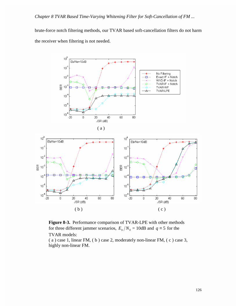
Chapter 8 TVAR Based Time-Varying Whitening Filter for Soft-Cancellation of FM ...
126
brute-force notch filtering methods, our TVAR based soft-cancellation filters do not harm
the receiver when filtering is not needed.
( a )
( b ) ( c )
Figure 8-3. Performance comparison of TVAR-LPE with other methodsfor three different jammer scenarios, 0NEb = 10dB and 5=q for the
TVAR models:( a ) case 1, linear FM, ( b ) case 2, moderately non-linear FM, ( c ) case 3,highly non-linear FM.

Chapter 8 TVAR Based Time-Varying Whitening Filter for Soft-Cancellation of FM ...
127
At high JSR, the TVAR based soft-cancellation methods provide consistent and
advantageous performance improvement for the linear FM case. The BER resulting from
the soft-cancellation methods is about an order of power less that resulting from the brute
force notch filter. This is attributed to the relatively flat top and adequate notch depth
associated with the soft-cancellation magnitude responses, as shown in Figure 8-1 and
Figure 7-3.
For the non-linear cases, Figure 8-3 (b) and (c) show that the processing gain of
the TVAR-WF and TVAR-LPE methods is limited, progressively more severely the more
severely non-linear the jammer. This effect can be reduced by increasing the polynomial
order (q ) of the TVAR model. For better performance of the TVAR based soft-
cancellation methods in case of highly non-linear FM jammers, a higher order q can be
used at the cost of computational complexity. To demonstrate this effect, Figure 8-4
shows the increasing performance of the soft-cancellation methods at high JSR for
increasing order q . Figure 8-3 (c) showed that with order 5=q , the filter suppresses the
jammer by about 30dB. Figure 8-4 shows that with orders 7=q and 8=q , the filter
suppresses the jammer by about 50dB and 60dB respectively. We also observe that the
TVAR-IF based notch filter is less sensitive to the order than the TVAR based soft-
cancellation filters. This suggest that if the order q is not high enough, the JSR
information captured by the model estimate is not accurate, and consequently, the
resulted TVAR-LPE filter does not match the data well.
In conclusion, the TVAR-LPE whitening method, similar to the TVAR-WF
method, provides improved performance over the notch filtering methods for the entire
range of JSR. They both utilize the full spectral information and are capable of

Chapter 8 TVAR Based Time-Varying Whitening Filter for Soft-Cancellation of FM ...
128
“adapting” to the data. The brute force notch filtering methods improve the overall DSSS
system performance when the jammer is strong, but deteriorate the system performance,
even with the exact IF, when JSR is low. Similar to the TVAR-WF, the TVAR-LPE does
not make the system worse than not filtering at all, regardless of JSR.
( a ) ( b )
( c ) ( d )
Figure 8-4. Effect of TVAR model basis function order on theperformance of TVAR based methods at high JSR for a highly non-linearFM jammer (case 3), 0NEb = 10dB:
( a ) 7=q , ( b ) 8=q , ( c ), 9=q , ( d ) 11=q .

Chapter 8 TVAR Based Time-Varying Whitening Filter for Soft-Cancellation of FM ...
129
8.4 Summary and Discussion
We proposed a time-varying filter for interference cancellation in DSSS
communications, which is a whitening filter based on TVAR modeling, named the TVAR
based linear prediction error (TVAR-LPE) filter. The proposed TVAR-LPE is a time-
varying extension of the AR model associated LPE filter in the stationary case. It
performs similarly to the TVAR-WF developed in Chapter 7, but is much less
complicated to implement than the TVAR-WF due to its short FIR structure and its direct
formulation from TVAR parameters, without the need for spectral factorization. The
TVAR-LPE and TVAR-WF methods both have distinct advantages in performance over
the IF estimate controlled brute-force notch filter in the DSSS interference cancellation
scenario.

Chapter 9 Summary and Suggestions for Future Work
130
Chapter 9
SUMMARY AND SUGGESTIONS FOR
FUTURE WORK
9.1 Summary
This dissertation is devoted to TVAR model based time-varying signal processing
and its applications to FM interference cancellation for DSSS communications. For
slowly time-varying environments, the adaptive signal processing methods can be applied
to track the variations. However, for the fast variation cases, an explicit description of the
variation is necessary for time-varying signal processing. Unfortunately, in practical
cases, such a description is rarely available. In this dissertation, we solve this problem
using the TVAR model. With the TVAR model, such a description is estimated from the
observed data record, and filtering is performed based on the identified TVAR model.
In the first part of the dissertation, Chapters 2 through 4, we studied TVAR based
IF estimation. In Chapter 2, we revealed the advantageous properties of TVAR based IF
estimation, which is expected to change the prevailing opinion about TVAR-IF that it is a
poor method for IF estimation. We demonstrated that TVAR-IF estimation is especially
advantageous for non-linear IF laws and short data records. Most IF estimation methods

Chapter 9 Summary and Suggestions for Future Work
131
deteriorate dramatically when the data SNR falls below some threshold. In Chapter 3, we
proposed a time-varying Prony method to improve the performance of TVAR-IF
estimation for low SNR cases. It is a time-varying extension of a simplified Prony
method for frequency estimation in the stationary case. Then in Chapter 4, we applied the
TVAR-IF estimates to time-varying notch filtering to reject FM jammers in DSSS
communications. It was demonstrated that the TVAR based IF estimate controlled notch
filter performs nearly the same as when using the exact IF, and much better than when
the notch filter is controlled by the prevailing WVD-IF estimate.
The second part of the dissertation, Chapters 5 through 7, focuses on time-varying
optimum filtering based on the TVAR model. A general framework for optimum
filtering, covering the Kalman filter and the Wiener filter, is provided in Chapter 5 with
emphasis on time-varying considerations. In Chapter 6, we developed the TVAR based
Kalman filter and TVAR based Wiener filters, with the latter including the causal version
and the ideal non-causal version. The TVAR-KF is directly derived from the Kalman
filter and therefore is the optimal causal filter assuming there are no modeling and/or
identification errors. By comparing against the TVAR-KF, we find the causal TVAR-WF
to be nearly optimal. Also, due to its non-causality, the non-causal TVAR-WF
significantly outperforms the causal optimal filter. In Chapter 7, we developed a method
of soft-cancellation of FM interference in DSSS communications based on the non-causal
TVAR-WF. The resulting filter is tailored to the full spectral information and is aimed at
minimum signal distortion. Unlike the brute-force notch filter, the TVAR-WF does not
harm the overall system performance (relative to not filtering at all) and yields desirable
performance improvements at both high and low JSR.
Chapter 9 Summary and Suggestions for Future Work
132
In Chapter 8, we developed another method of soft-cancellation of FM jammers
in DSSS communications based on the TVAR model. It is aimed at flatness of the output
spectrum, and the resulting filter is the TVAR based linear prediction error (TVAR-LPE)
filter. Similar to the TVAR-WF method, the TVAR-LPE yields the desired performance
over the entire range of JSR. Unlike the TVAR-WF and TVAR-IF methods, the TVAR-
LPE is formed from the TVAR parameters directly without any further calculation.
Another advantage of the TVAR-LPE filter is its short FIR structure, which further
simplifies implementation.
9.2 Suggestions for Future Work
The reported research was concentrated on developing TVAR based signal
processing methods and applying them to reject FM interference in DSSS
communications. Future research may develop along two major directions: theoretical
research and application and implementation issues. In the theoretical realm, some
performance analysis of the proposed methods may be helpful to better understand and
apply the proposed methods. The questions to be answered include, for example, how
theoretical analysis is feasible and how the WVD and WS based TVWF [21] relates to
our TVAR-WF and if it would be useful in predicting limitations on the practical use of
TVAR modeling. In terms of application and implementation aspects, one may evaluate
the computational load required to implement each method for given scenarios and widen
the realm of applications. Based on a complexity versus performance tradeoff, one may
provide advice on selection of time-varying filter methods. One may also study system
design issues for applications of the proposed methods. For example, the TVAR-WF and

Chapter 9 Summary and Suggestions for Future Work
133
TVAR-LPE methods are based on treating the DSSS signal as an approximately white
signal. From this point of view, a small over-sampling ratio (samples per chip) is desired.
Other aspects of system design may desire a larger over-sampling ratio. The question of
how to choose the sampling rate or design a multi-rate system may become a practical
issue in a real-world application.
We have focused on the application of the proposed TVAR based filtering
methods to the problem of FM interference rejection in DSSS communications. One may
apply the TVAR based methods to other engineering and research scenarios, such as in
speech enhancement, seismic signal processing, radar/sonar signal processing, and
biomedical and biophysical signal analysis and processing. In the communication field,
one may apply the proposed methods to reject co-channel interference for FM
communications or perform multiple-FM demodulation. One may also study the use of
these TVAR based methods, or modifications thereof, to reject a frequency-hopping
jammer in DSSS communications. It is further suggested that the TVAR-KF or a similar
TVAR based Kalman smoother (with delay) be evaluated for the interference suppression
problem.

Appendix
134
Appendix A
Wigner-Ville Distribution (WVD) and WVD Peak Based
IF Estimation
A-1 Wigner-Ville Distribution (WVD)
The Wigner-Ville Distribution (WVD) is defined for both continuous signals and
limited-length discrete-time sequences. Since this dissertation concerns signal processing
for a discrete-time record (block) only, we limit our discussion to such cases.
Let )(tx be a discrete-time series of length N, with time-index 1...,,1,0 −= Nt .
For simplicity of presentation, we assume that the length N of the data record is even. We
define the "instantaneous correlation function" as:
)()(),( mtxmtxmtc −+= ∗ (A-1)
where zero-values are assumed for x(t) outside of the data record and m is the "half of
lag" which takes integer values from 22
Nm
N <≤− . Then the discrete Wigner-Ville
Distribution (WVD) is defined as the discrete Fourier transform (DFT) of the ),( mtc
with respect to the lag m2 for each time instant 1...,,1,0 −= Nt , which is
∑ π−=m
NkmjemtcktW )2(2),(2),( (A-2)
where k is the discrete frequency. For unity sampling rate, which we have assumed, the
corresponding continuous frequency is N
kf
2= .
Note that, from t in )(tx to m2 in ),( mtc , decimation by 2 is involved and,
consequently, for each given time instant t , the WVD ),( ktW corresponds to an aliased
power spectrum of the signal. If the original data is real-valued, it is usually converted to
the analytic signal, which has a single-sided spectrum. The output of the real-to-analytic
transform has the original signal as its real part and the Hilbert transform of the real part
as its imaginary part.

Appendix
135
A-2 WVD Based IF Estimation (WVD-IF)
Assume that the signal )(tx consists of only one signal component. Then the
instantaneous frequency (IF) of the signal component can be estimated by searching for
the frequency peak position of its WVD ),( ktW for each time instant t . The estimate can
be expressed in terms of an estimate of the continuous frequency )(ˆ tf as
{ }),(maxarg2
1)(ˆ ktW
Ntf
k
= (A-3a)
or in terms of an estimate of the discrete frequency index )(ˆ tk :
{ }),(maxarg)(ˆ ktWtkk
= (A-3b)
The IF estimate takes values from a set of discrete values with quantization
interval N2
1. For short data records, the estimate is poor due to the frequency
quantization. This effect can be reduced by padding zeros to the data )(tx or, more
efficiently, padding zeros to ),( mtc along the m axis. The latter means increasing the
number of points in the DFT contained in (A-2).
A-3 Example of WVD and WVD-IF
For a 32-point data record of a linear chirp signal in white noise at SNR=20dB,
we compute its WVD and WVD-IF. The IF law is 31,,1,0,01.01.0)( �=+= tttf . The
data is the same as that used in Section 2.2.2, as shown in Figure 2-1. We compute the
WVD in two versions, without zero-padding, which uses a 32-point DFT and is denoted
as WVD(32), and with zero-padding to 64-points, which uses a 64-point DFT and is
denoted as WVD(64). The result is shown in Figure A-1 in the top and middle rows, with
the left column for WVD(32) and the right column for WVD(64). The IF estimates
resulting from the peak locations in the WVD estimates are shown below also. The finer
frequency quantization interval associated with the WVD(64) IF estimates is observable
in the increased smoothness of the latter. The WVD-IF is improved by zero-padding at
the cost of computational effort. The IF estimates near the ends of the data record are
less reliable than in the center. This is due to the fact that there are fewer data samples

Appendix
136
available for computing the "instantaneous correlation function" ),( mtc near the data
ends. This is referred to as the end effects of the WVD based IF estimation.
t
f
0 10 20 300
0.1
0.2
0.3
0.4
0.5
t
f
0 10 20 300
0.1
0.2
0.3
0.4
0.5
Figure A-1. Example of WVD (top and middle) and WVD-IF (bottom)based on WVD(32) (left) and WVD(64) (right), a linear FM signal inwhite nose at SNR=20dB.

Appendix
137
Appendix B
Evolutionary Spectrum Theory and its Relation to this Work
B-1 Review of Priestley’s Evolutionary Spectrum Theory [24]
Let x(t) be a non-stationary time series that admits a representation of the form
)()()( ωωφπ
πdZtx t∫−
= , ...,,2,1,0 ±±=t (B-1)
where )(ωZ is an orthogonal process and ]|)([| 2ωdZE plays the same role as the power
spectrum in the Fourier analysis of stationary processes (where the kernel function family
is taken as tjt e ω=ωφ )( ). Suppose that )(ωφt can be expressed in the form of a jointly
frequency- and amplitude-modulated (FM-AM) function
tjtt eA )()()( ωθωωφ = (B-2)
where the amplitude-modulating function )(ωtA has its peak Fourier spectrum at zero
frequency. When )(ωφ t is considered as a function of t, it is called an oscillatory
function if it can be written in the form indicated in (B-2). If there exists a family of
oscillatory functions { )(ωφ t } such that the process { )(tx } can be expressed in the form
(B-1), { )(tx } is called an oscillatory process.
Further assuming that )(ωθ in (B-2) is a single-valued function of ω , by
transforming the variable in the integral in (B-1) from ω to )(ωθ and adjusting the terms
)(ωtA and )(ωZ , it is possible to write
)()()( ωω ωπ
πdZeAtx tj
t∫−= , ...,,2,1,0 ±±=t (B-3)
with
)(]|)([| 2 ωµω ddZE = (B-4)
For a given family of oscillatory functions, })({)}({ tjtt eA ωωωφ = , in terms of
which an oscillatory process { )(tx } can be expressed in the form (B-3), the evolutionary
power spectrum )(ωtdH , at time t, of the oscillatory process { )(tx } with respect to the
specific family of oscillatory functions, is then defined by

Appendix
138
)(|)(|)( 2 ωµωω dAdH tt = , πωπ ≤≤− (B-5)
For the special case when { )(tx } is stationary, if the family of oscillatory
functions })({)}({ tjtt eA ωωωφ = is chosen to be the family of complex exponential
functions, the evolutionary power spectrum )(ωtdH reduces to the standard Fourier
power spectrum.
Priestley suggested a two-stage procedure for estimating the evolutionary
spectrum from a data record. For frequency sample 0ω , the first step is to pass the data
through a linear bandpass filter centered at 0ω , and, the second step is to estimate the
time-varying power at 0ω by averaging the squared value of the filter output over a
sliding (short-time) temporal window. In other words, Priestley’s evolutionary spectral
estimation is based on a filter-bank (frequency-domain windowing) followed by short-
time power estimation (time-domain windowing).
B-2 Relation of Priestley’s Evolutionary Spectrum Theory to this Work
In this research, the data is modeled with a TVAR model, and time-varying
characteristics are represented in the TVAR parameters. In many cases, such as time-
varying filter design, we can use the model parameters themselves without estimating a
two-dimensional evolutionary spectrum (also called a time-frequency distribution or
time-varying spectrum). If needed, the time-varying spectrum estimation corresponding
to the TVAR model can be evaluated in a straightforward manner from the TVAR
parameters, as expressed in (6-18), in a fashion similar to parametric spectral estimation
for stationary processes [30].
Since Priestley’s evolutionary spectral estimation involves frequency-domain and
time-domain windowing, it is not suitable for short data records and fast-varying signals.
In contrast, our method models the entire data record or data block with the time-varying
characteristics incorporated by the model. In other words, we capture time-varying
information by model identification, rather than by short-time windowing. Consequently,
the proposed work may be more suitable for short data records and fast-varying non-
stationarity.

Appendix
139
Although our method of capturing time-varying characteristics is distinct from
that of Priestley’s evolutionary spectrum estimation, our definition of the parametric
time-varying spectrum, as expressed in (6-18), can be viewed as a special case under the
umbrella of Priestley’s evolutionary spectral theory, as explained next.
We model the data as the output of a linear time-varying system, G(t, z), excited
by a stationary white noise e(t) with power 2eσ , where
∑==
=
−p
i
ii zta
ztAztG
0)(
1
),(
1),( , 10 ≡a (B-6)
We denote the impulse response of G(t, z) as ),( τtg , representing the response at
time t contributed by an impulse input at time )( τ−t :
∑∞
=
−=0
),(),(i
izitgztG (B-7)
Then, we can express the data )(tx in terms of ),( τtg and e(t):
∑−∞=
−=t
i
ieittgtx )(),()( (B-8)
where e(t) is stationary and white, and therefore can be expressed in terms of Fourier
analysis. Following the notation of Priestley’s evolutionary spectrum theory, we can
write the Fourier analysis of e(t):
)()( ω∫= ππ−
ω dZete tj (B-9)
where )(ωZ is a process satisfying
πωσωωδωω2
)()]()([ 121121
ddZdZE e−=∗ (B-10)
Substituting (B-9) into (B-8), we have an expression for the data in the form of (B-3):
)(),()( wdZeetGtx tjj∫= ππ−
ωω (B-11)
The evolutionary spectrum defined in (B-5) is then,
)(|),(|)( 2 ωµ=ω ω detGdH jt (B-12)
From (B-4) and (B-10), we have
πωσωµ
2)( 2 d
d e= (B-13)

Appendix
140
and from (B-6), we have
πωσ
=ωω 2|),(|
)(2
2 d
etAdH
je
t (B-14)
This is equivalent to our time-varying spectrum (6-18) evaluated on the unit circle with
ω= jez .

Bibliography
141
BIBLIOGRAPHY
[1] G. F. Boudreaux-Bartels and T. W. Parks, “Time-varying filtering and signalestimation using Wigner Distribution synthesis techniques,” IEEE Trans. ASSP,vol. ASSP-34, no. 3, pp. 442-451, June 1986.
[2] W. Kozek and F. Hlawatsch, “A comparative study of linear and nonlinear time-frequency filters,” Proc. IEEE Int. Symp. Time-Frequency Time-Scale Analysis,Oct. 1992 (TFTS’92), Victoria, Canada, pp. 163-166.
[3] B. Boashash, “Time-frequency signal analysis,” in Advances in Spectrum Analysisand Array Processing, vol. 1, S. Haykin Ed., Prentice Hall, New York, 1990.
[4] L. Cohen, “Time-frequency distributions,” Proc. IEEE, vol. 77, pp. 941-981, 1989.
[5] W. Krattenthaler and F. Hlawatsch, “Time-frequency design and processing ofsignals via smoothed Wigner distributions,” IEEE Trans. Signal Processing, vol.41, no. 1, pp. 278-287, Jan. 1993.
[6] M. R. Portnoff, “Time-frequency representation of digital signals and systemsbased on short-time Fourier analysis,” IEEE Trans. ASSP, vol. 28, no. 2, pp. 55-69,Feb. 1980.
[7] R. Bourdier, J. F. Allard, and K. Trumpf, “Effective frequency response and signalreplica generation for filtering algorithms using multiplicative modifications of theSTFT,” Signal Processing, vol. 15, no. 2, pp. 193-201, Sept. 1988.
[8] I. Daubechies, “Time-frequency localization operators: A geometric phase spaceapproach,” IEEE Trans. Information Theory, vol. 34, no. 4, pp. 605-201, July 1988.
[9] S. Farkash and S. Raz, “Time-variant filtering via the Gabor expansion,” SignalProcessing V: Theories and Applications. Elsevier, 1990, pp. 509-512.
[10] I. Daubechies and T. Paul, “Time-frequency localization operators: A geometricphase space approach: II. The use of dilations,” Inverse Problems, no. 4, pp.661-680, 1988.
[11] F. Hlawatsch and W. Kozek, “Time-frequency projection filters and time-frequencysignal expansions,” IEEE Trans. Signal Processing, vol. 42, no. 12, pp. 3321-3334,Dec. 1994.
[12] F. Hlawatsch, W. Kozek, and W. Krattenthaler, “Time-frequency subspaces andtheir application to time-varying filtering,” IEEE ICASSP’90, pp. 1607-1610, Apr.1990, Albuquerque, NM.
[13] F. Hlawatsch and W. Kozek, “Time-frequency analysis of linear signal spaces,”IEEE ICASSP’91, pp. 2045-2048, May 1991, Toronto, Canada.
[14] R. G. Shenoy and T. W. Parks, “The Weyl correspondence and time-frequencyanalysis,” IEEE Trans. Signal Processing, vol. 42, no. 2, pp. 318-332, Feb. 1994.
[15] W. Kozek, “Time frequency signal processing based on the Wigner-Weylframework,” Signal Processing, vol. 29, no. 1, pp. 77-92, Oct. 1992.

Bibliography
142
[16] B. A. Weisburn and T. W. Parks, “Design of time frequency strip filters,”Conference Record of the 29th Asilomar Conference on Signals, Systems andComputers, pp. 930-934, Oct. 1995.
[17] B. A. Weisburn and R. G. Shenoy, “Time-frequency strip filters,” IEEEICASSP’96, pp. 1411-1414, Atlanta, GA, May 1996.
[18] M. A. Kutay, H. M. Ozaktas, L. Onural, and O. Arikan, “Optimal filtering infractional Fourier domains,” IEEE ICASSP’95, pp. 937-940, Detroit, MI, May1995.
[19] H. L. Van Trees, Detection, Estimation, and Modulation Theory, Part 1: Detection,Estimation, and Linear Modulation Theory, John Wiley and Sons, Inc., New York,1968.
[20] N. A. Abdrabbo and M. B. Priestley, “Filtering non-stationary signals,” RoyalStatistical Society Journal, Vol. 31, pp. 150-159, 1969.
[21] H. Kirchauer, F. Hlawatsch, and W. Kozek, “Time-frequency formulation anddesign of nonstationary Wiener filters,” IEEE ICASSP’95, pp. 1549-1552, Detroit,MI, May 1995.
[22] A. A. Beex and M. Xie, “Time-varying filtering via multiresolution parametricspectral estimation,” IEEE ICASSP’95, pp. 1565-1568, Detroit, MI, May 1995.
[23] H. A. Khan and L. F. Chaparro, “Non-stationary Wiener filtering based onevolutionary spectral theory,” IEEE ICASSP’97, pp3677-3680, Munich, Germany,April 1997,
[24] M. B. Priestley, Non-linear and non-stationary time-series analysis, AcademicPress, San Diego, CA, 1988.
[25] M. Xie and A. A. Beex, “Multiresolution parametric spectral estimation,” 26th
Southeastern Symposium on System Theory, Athens, OH, pp. 432-436, March1994.
[26] M. Xie, Signal Decomposition for Nonstationary Processes, Ph.D. dissertation,Virginia Polytechnic Institute and State University, Blacksburg, VA, 1995.
[27] P. Shan and A. A. Beex, “Time-varying Wiener filtering based on a time-varyingAR model,” 8th IEEE Digital Signal Processing Workshop, Vol. 1, ppr. # 52, Aug.1998, Bryce Canyon, Utah.
[28] M. G. Hall, A. V. Oppenheim, and A. S. Willsky, “Time-varying parametricmodeling of speech,” Signal Processing, vol. 5, no. 3, pp. 267-285, May 1983.
[29] Y. Grenier, “Time-dependent ARMA modeling of nonstationary signals,” IEEETrans. ASSP, vol. 31, no. 4, pp. 899-911, Aug. 1983.
[30] S. Kay, Modern Spectral Estimation, Prentice Hall, Englewood Cliffs, NJ, 1988.
[31] B. Boashash, “Estimating and interpreting the instantaneous frequency of a signal -part 2: algorithms and applications,” Proc. of IEEE, vol. 80, no. 4, pp. 540-568,April 1992.

Bibliography
143
[32] F. Hlawatsch and G. F. Boudreaux-Bartels, “Linear and quadratic time-frequencysignal representations,” IEEE Signal Processing Magazine, vol. 9, no. 2, pp. 21-67,April 1992.
[33] P. Rao and F. J. Taylor, “Estimation of the instantaneous frequency using thediscrete Wigner distribution,” Electronics Letters, vol. 26, no. 4, pp. 246-248, Feb.1990.
[34] P. Shan and A. A. Beex, “High-Resolution Instantaneous Frequency EstimationBased on Time-Varying AR Modeling,” IEEE-SP the 4th International Symposiumon Time-Frequency and Time-Scale Analysis (TFTS’98), pp. 109-122, Pittsburgh,PA, Oct. 1998.
[35] H. Cohen, G. F. Boudreaux-Bartels, and S. Kadambe, “Tracking of unknown non-stationary chirp signals using unsupervised clustering in the Wigner distributionspace,” IEEE ICASSP’88, pp. 2180-83, Seattle, WA, May 1988.
[36] K. C. Sharman and B. Friedlander, “Time-varying autoregressive modeling of aclass of nonstationary signals,” Proc. ICASSP’84, San Diego, CA, vol. 2, pp.22.2.1-22.2.4, March 1984.
[37] C. W. Therrien, Discrete Random Signals and Statistical Signal Processing,Prentice Hall, Englewood Cliffs, NJ, 1992.
[38] S. Haykin, Adaptive Filter Theory, Prentice Hall, Upper Saddle River, NJ, 1996.
[39] L. Ljung, System Identification: Theory for the User, Chapter 5, Prentice Hall,Upper Saddle River, NJ, 1987.
[40] M. K. Tsatsanis and G. B. Giannakis, “Time-varying system identification andmodel validation using wavelets,” IEEE Trans. on Signal Processing, vol. 41, no.12, pp. 3512-23, Dec. 1993.
[41] T. S. Rao, “The fitting of nonstationary time-series models with time-dependentparameters,” J. Royal Statist. Soc. Series B, vol. 32, no. 2, pp. 312-322, 1970.
[42] A. Duel-Hallen, J. Holtzman, and Z. Zvonar, “Multiuser detection for CDMAsystems,” IEEE Personal Communications, April 1995, pp.46-58.
[43] S. Moshavi, “Multi-user detection for DS-CDMA communications,” IEEECommunications Magazine, Oct. 1996, pp.124-136.
[44] L. B. Milstein and R. A. Iltis, “Signal processing for interference rejection inspread spectrum communications,” IEEE ASSP Magazine, April 1986, pp. 18-31.
[45] M. Medley, G. Saulnier, and P. Das, “Applications of the wavelet transform inspread spectrum communications,” Proc. SPIE, Wavelets Applications, Orlando,FL, Apr. 1994, pp. 54-68.
[46] L. Milstein, “Interference suppression to aid acquisition in direct-sequence spread-spectrum communications,” IEEE Trans. Communications, vol. 36, pp. 1200-1207,Nov. 1988.

Bibliography
144
[47] M. G. Amin, A. R. Lindsey, and C. Wang, “On the application of time-frequencydistributions in the excision of pulse jamming in spread spectrum communicationsystems,” IEEE Workshop on SSAP, pp. 152-155, Greece, June 1996.
[48] M. G. Amin, “Interference mitigation in spread spectrum communication systemsusing time-frequency distributions,” IEEE Trans. Signal Processing, vol. 45, no. 1,pp.90-101, Jan. 1997.
[49] S. R. Lach, M. G. Amin, and A. R. Lindsey, “Broadband nonstationary interferenceexcision for spread spectrum communications using time-frequency synthesis,”IEEE ICASSP’98, pp. 3257-3260, Seattle, WA, May 1998.
[50] A. Bultan and A. N. Akansu, “A novel time-frequency exciser in spread spectrumcommunications for chirp-like interference,” IEEE ICASSP’98, pp. 3265-3268,Seattle, WA, May 1998.
[51] A. Bultan, “A four-parameter atomic decomposition of chirplets,” IEEEICASSP’97, pp. 3625-3628, Munich, Germany, April 1997.
[52] S. Mallat and Z. Zhang, “Matching pursuits with time-frequency dictionaries,”IEEE Trans. Signal Processing, vol. 41, pp. 3397-3415, Dec. 1993.
[53] R. Kumaresan, D. W. Tufts, and L. L. Scharf, “A Prony method for noisy data:choosing the signal components and selecting the order in exponential signalmodels,” Proceedings of IEEE, vol. 72, no.2, pp. 230-233, February 1984.
[54] J. G. Proakis, Digital Communications, McGraw-Hill, New York, NY, 1995.
[55] L. W. Couch II, Digital and Analog Communication Systems, MacmillanPublishing Co., New York, NY, 1993.
[56] R. P. Hocking and L. L. Leslie, “Selection of the best subset in regressionanalysis,” Technometrics, vol. 9, pp. 537-540, 1967.
[57] P. Shan and A. A. Beex, “FM interference suppression in spread spectrumcommunications using time-varying autoregressive modeling based instantaneousfrequency estimation,” IEEE ICASSP’99, vol. V, pp. 2559-62, Phoenix, AZ, Mar.1999.
[58] S. R. Lach, A. R. Lindsey, and M. G. Amin, “A comparison between two time-frequency bilinear transforms for interference excisions in spread spectrumcommunications,” IEEE DSP Workshop’98, ppr # 85, Bryce Canyon, UT, 1998.
[59] D. Wei, D. S. Harding, and A. C. Bovik, “Interference suppression in direct-sequence spread-spectrum communications using the discrete Gabor transform,”IEEE DSP Workshop’98, ppr # 61, Bryce Canyon, UT, Aug. 1998.
[60] C. Wang and G. Amin, “Performance analysis of instantaneous frequency-basedinterference excision techniques in spread spectrum communications,” IEEE Trans.SP, vol. 46, no. 1, pp. 70-82, Jan. 1998.
[61] L. Liporace, “Linear estimation of nonstationary signals,” J. Acoustics Soc. Amer.,vol. 58, no. 6, pp. 1268-1295, Dec. 1975.

Bibliography
145
[62] D. C. Rife and R. R. Boorstyn, “ Single tone parameter estimation from discrete-time observation,” IEEE Trans. Information Theory, vol. 20, pp. 591-598, 1974.
[63] M. Morf, B. Dickinson, T. Kailath, and A. Vieira, “Efficient solution of covarianceequations for linear prediction,” IEEE Trans. ASSP, vol ASSP-25, no. 5, pp. 429-433, 1977.
[64] B. Friedlander, T. Kailath, M. Morf, and L. Ljung, “Extended Levinson andChandrasekar equations for discrete-time linear estimation problems,” IEEE Trans.Automatic Control, vol. AC-23, no. 4, pp. 653-659, 1978.
[65] A. A. Beex and P. Shan, “A time-varying Prony method for instantaneousfrequency estimation at low SNR,” 1999 IEEE International Symposium onCircuits and Systems, vol. III, pp. 5-8, Orlando, FL, May 1999.
[66] C. Wang, M. G. Amin, and A. Lindsey, “Open loop adaptive filtering forinterference exision in spread spectrum systems," Conference Record of the 31stAsilomar Conf. on Signals, Systems & Computers, pp. 520-524, Pacific Grove,CA, Nov. 1997.
[67] P. Shan and A. A. Beex, “Time-varying filtering using full spectral information forsoft-cancellation of FM interference in spread spectrum communications,”Proceedings of the 2nd IEEE Workshop on Signal Processing Advances in WirelessCommunications (SPAWC’99), pp.321-324, Annapolis, MD, May 1999.
[68] R. J. Wang, "The Determination of Optimum Gate Lengths for Time-VaryingWiener Filtering" Geophysics, vol. 34, no. 5, pp. 683-695, Oct. 1969.
[69] N. Wiener, Extraction, Interpolation, and Smoothing of Stationary Time Series,with Engineering Applications, MIT Press, Cambridge, MA, 1949.
[70] M. G. Amin, C. Wang, and A. R. Lindsey, “Optimum interference excision inspread spectrum communications using open-loop adaptive filters,” IEEE Trans.Signal Processing, vol. 47, no. 7, pp. 1966-1976, July 1999.

146
Vita
Peijun Shan received the MS degree in Electrical Engineering in 1989 from
Xidian University, formerly the Northwest Telecommunications Engineering Institute,
Xi’an, China. Next he was employed as a research and development engineer by the same
university where he worked on various projects. During that period, he was awarded two
invention patents and published/presented about 20 papers. Later, he was employed by
GE Medical Systems before he came to the U.S. for higher education. As a GRA
(graduate research assistant) at Virginia Tech, he worked from 1996 to 1998 on EEG
processing, analysis and visualization in the Center for Brain Research and Information
Sciences Radford University, Radford, Virginia. He also instructed senior-level DSP
Laboratory at Virginia Tech.
In his Ph.D. program, he concentrated on communications and signal processing
and conducted research in the DSP Research Laboratory at Virginia Tech. His current
research interests are in time-varying signal processing, interference cancellation and
spread spectrum communications. In July 1999, he joined RF Micro Devices Inc.,
Greensboro, North Carolina, as a Senior Design Engineer working on communication
baseband subsystem design. He is a member of IEEE Signal Processing Society and
Communications Society.