Simulations in Statistics

14-1Copyright © 2010 Pearson Education, Inc. Publishing as Prentice Hall

Simulation

Chapter 14


Not all real-word problems can be solved by applying a specific techniques and then performing calculations.

Some situations are too complex to be represented by precise techniques, and the alternative form of analysis is simulation.

Simulation

14-3

■The Monte Carlo Process

■Computer Simulation with Excel Spreadsheets

■Simulation of a Queuing System

■Continuous Probability Distributions

■Statistical Analysis of Simulation Results

■Crystal Ball

■Verification of the Simulation Model

■Areas of Simulation Application

Chapter TopicsCopyright © 2010 Pearson Education, Inc. Publishing as Prentice Hall

14-4

■Analogue simulation replaces the original physical system with an analogous physical system that is easier to manipulate.

■In computer mathematical simulation a system is replaced with a mathematical model that is analyzed with the computer.

■Simulation offers a means of analyzing very complex systems that cannot be analyzed using the other management science techniques.

Examples: weightlessness was simulated using rooms filled with water; wind tunnels simulated conditions of flight; treadmills simulated automobile tire wear, etc.

Overview Copyright © 2010 Pearson Education, Inc. Publishing as Prentice Hall

14-5

■A large proportion of the applications of simulations are for probabilistic models.

■We will present simplified simulation models.

■The Monte Carlo is a technique for selecting numbers randomly from a probability distribution for use in a trial (computer run) of a simulation model.

■Monte Carlo is not a type of simulation model, but a mathematical process used within a simulation.

■The basic principle behind the process is the same as in the operation of gambling devices in casinos (such as those in Monte Carlo, Monaco).

Monte Carlo ProcessCopyright © 2010 Pearson Education, Inc. Publishing as Prentice Hall

14-6

The purpose of the Monte Carlo process is to generate the random variable, representing the demand, by sampling from the probability distribution P(x).

The partitioned roulette wheel replicates the probability distribution for demand if the values of demand occur in a random manner.

Let take a first example:

Monte Carlo ProcessCopyright © 2010 Pearson Education, Inc. Publishing as Prentice Hall


Simulation Example

Use Monte Carlo Process

14-8

Table 14.1 Probability Distribution of Demand for Laptop PC’s

Example: ComputerWorld demand data for laptops selling for $4,300 over a period of 100 weeks.

Monte Carlo ProcessUse of Random Numbers

Copyright © 2010 Pearson Education, Inc. Publishing as Prentice Hall

14-9

Figure 14.1 A Roulette Wheel for Demand



14-10

Figure 14.2Numbered Roulette Wheel


When the wheel is spun, the actual demand for PCs is determined by a number at rim of the wheel.


The segment at which the wheel stops indicates demand for one week.

14-11

Table 14.2 Generating Demand from Random Numbers



Use cumulative probability for ranges of random numbers.

Demand

Cumulative

0 0.20

1 0.60

2 0.80

3 0.90

4 1.00

14-12

Select from a random number table (computer generated):

Table 14.3 Delightfully Random Numbers



14-13

The selection of random numbers simulates demand for a period of time.

These random numbers are all equally likely to occur, just as if we spun a wheel.

Compute demand for each random number, using the range, and compute revenue.



14-14



Table 14.4

Demand

Cumulative

0 0.20

1 0.60

2 0.80

3 0.90

4 1.00

14-15

Estimated average demand:

Average demand: 2.07 laptop PCs per week.

Estimated average revenue

Average revenue: $8,886.67.



07.21531

weeksofnumberdemandtotal

67.886,815

300,133 weeksofnumber

revenuetotal

14-16

Average demand could have been calculated analytically:

where = demand value i

= probability of demand

= the number of different demand values

therefore:



n

iii xxPxE

1)()(

weekpersPC

xE

'5.1

)4)(10(.)3)(10(.)2)(20(.)1)(40(.)0)(20(.)(

ix)( ixP

n

14-17

The more periods simulated, the more accurate the results.

Simulation results will not equal analytical results unless enough trials have been conducted to reach steady state.

Often is difficult to validate results of simulation - that true steady state has been reached and that simulation model truly replicates reality.

When analytical analysis is not possible, there is no analytical standard of comparison thus making validation even more difficult.



14-18

As simulation models get more complex they become impossible to perform manually.

In simulation modeling, random numbers are generated by a mathematical process instead of a physical process (such as wheel spinning).

Random numbers are typically generated on the computer using a numerical technique and thus are not true random numbers but pseudorandom numbers.

Computer Simulation with Excel SpreadsheetsGenerating Random Numbers (1 of 2)


14-19

Artificially created random numbers must have the following characteristics:

1. The random numbers must be uniformly distributed (each has an equal chance to be selected).

2. The numerical technique for generating the numbers must be efficient (not degenerating into a constant; no recycle).

3. The sequence of random numbers should reflect no pattern.

Computer Simulation with Excel SpreadsheetsGenerating Random Numbers (2 of 2)


14-20

Exhibit 14.1

Simulation with Excel Spreadsheets(numbers between 0 and 1, not integers)


14-21

Exhibit 14.2

Simulation with Excel SpreadsheetsCopyright © 2010 Pearson Education, Inc. Publishing as Prentice Hall

14-22

Exhibit 14.3

Simulation with Excel Spreadsheets (100 RN)


14-23

Revised ComputerWorld example; order size of one laptop each week.

Computer Simulation with Excel SpreadsheetsDecision Making with Simulation (1 of 2)


Exhibit 14.4

14-24

Order size of two laptops each week.

Computer Simulation with Excel SpreadsheetsDecision Making with Simulation (2 of 2)


Exhibit 14.5

14-25


Simulation of a Queuing System

14-26


Queuing SystemWaiting in queues – waiting lines – most

common occurrences in everyone’s life. Quick service is an important aspect of quality custom service.

Single – Server Waiting line system (simplest form of QS)

• Queue Discipline (ex. first-come, first-served)

• Calling Population (finite or infinite)• Arrival Rate: λ – mean (ex. Poisson

distribution)• Service Rate: µ - mean (ex. Exponential)Need: λ < µ ; Utilization factor: U= λ / µ

(ie. U < 1)Solution: adding another employee or

adding a new check out counter.Multiple – Server Waiting line – can be in

sequence.

Simulation

14-27

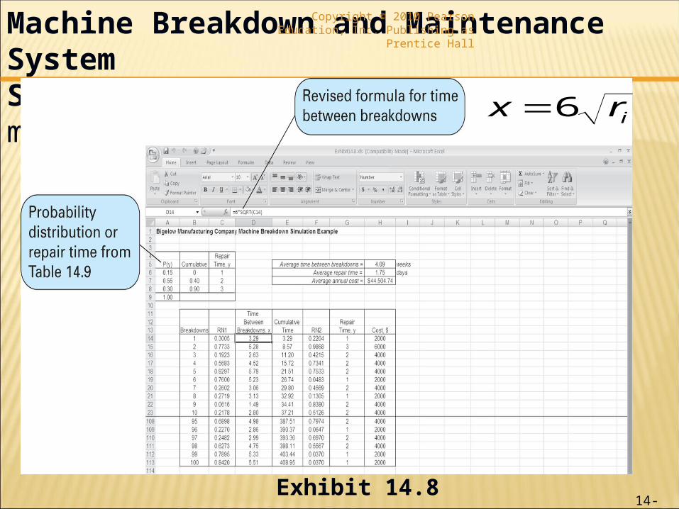
Burlingham produces denim. The main step in production process is dyeing the yarn.

Once batches arrive, it takes some time to complete the dyeing process.

The following table present the distribution of arrival intervals and distribution of service time.

Simulation of a Queuing SystemBurlingham Mills Example


14-28

Table 14.5 Distribution of Arrival Intervals

Table 14.6 Distribution of Service Times



14-29

Average waiting time = 12.5days/10 batches = 1.25 days per batchAverage time in the system = 24.5 days/10 batches = 2.45 days per batch

Simulation of Queuing SystemBurlingham Mills Example


Arrival

Range r1

1.0 1 - 20

2.0 21 - 60

3.0 61 - 90

4.0 91 – 99, 00

Service Range r2

0.5 1 – 20

1.0 21 – 70

2.0 71 – 99,00

14-30


■ Results may be viewed with skepticism.

■ Ten trials do not ensure steady-state results.

■ Starting conditions can affect simulation results.

■ If no batches are in the system at start, simulation must run until it replicates normal operating system.

■ If system starts with items already in the system, simulation must begin with items in the system.


14-31

Exhibit 14.6

Computer Simulation with ExcelBurlingham Mills Example


14-32


Continuous Probability Distribution

Simulation

14-33

Continuous Probability DistributionsCopyright © 2010 Pearson Education, Inc. Publishing as Prentice Hall

40,8

)( xx

xf

16281

81

8)(

2

0

2

00

xxdxxdx

xxF

xxx

16

2xr

A continuous function must be used for continuous distributions.

Example:

where x is the time in minutes.

Cumulative probability of x:

Let F(x) be the random number r:

By generation a random number r, a value x for “time” is determined.

14-34


Simulation Example

For Continuous Distribution

14-35

Machine Breakdown and Maintenance SystemSimulation

Bigelow Manufacturing Company must decide if it should implement a machine maintenance program at a cost of $20,000 per year that would reduce the frequency of breakdowns and thus time for repair which is $2,000 per day in lost production.

A continuous probability distribution of the time between machine breakdowns:

where x = weeks between machine breakdowns.

Since we have

the value of x for a given value of ri.


40,8

)( xx

xf

irx 416

2xr

14-36

Table 14.8Probability Distribution of Machine Repair Time



14-37

Table 14.9

Machine Breakdown and Maintenance SystemSimulation (3 of 6)

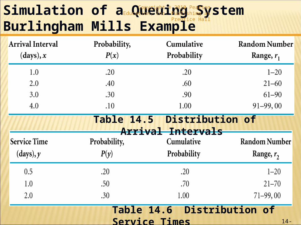
Revised probability of time between machine breakdowns:

weeks where x = weeks between machine breakdowns.

The equation for generating x, given random number r1 is :


60,8

)( xx

xf

irx 6

14-38

Table 14.9Revised Probability Distribution of

Machine Repair Time with the Maintenance Program



14-39

Table 14.10

Machine Breakdown and Maintenance SystemSimulation - without maintenance program

(total annual repair cost of $84,000):


irx 4

14-40

Table 14.11

Machine Breakdown and Maintenance SystemSimulation - with maintenance program

(total annual repair cost of $42,000):


irx 6

14-41


Results and caveats:■ Implement maintenance program since cost

savings appear to be $42,000 per year and maintenance program will cost $20,000 per year.

■ However, there are potential problems caused by simulating both systems only once.

■ Simulation results could exhibit significant variation since time between breakdowns and repair times are probabilistic.

■ To be sure of accuracy of results, simulations of each system must be run many times and average results computed.

■ Efficient computer simulation required to do this.


14-42

Exhibit 14.7

Machine Breakdown and Maintenance SystemSimulation with Excel - Original machine breakdown example:


irx 4

14-43

Exhibit 14.8

Machine Breakdown and Maintenance SystemSimulation with Excel - with maintenance program.


irx 6

14-44

Outcomes of simulation modeling are statistical measures such as averages.

Statistical results are typically subjected to additional statistical analysis to determine their degree of accuracy.

Confidence limits are developed for the analysis of the statistical validity of simulation results.

Statistical Analysis of Simulation Results (1 of 2)


14-45

Formulas for 95% confidence limits:

upper confidence limit

lower confidence limit

where is the mean and s the standard deviation from a sample of size n from any population.

We can be 95% confident that the true population mean will be between the upper confidence limit and lower confidence limit.

)/)(.( nsx 961

)/)(.( nsx 961

x

Statistical Analysis of Simulation Results (2 of 2)


14-46

Simulation Results - Statistical Analysis with Excel - with maintenance program.


Exhibit 14.9

14-47

Simulation ResultsStatistical Analysis with Excel (2 of 3)


Exhibit 14.10

14-48

Exhibit 14.11

Simulation ResultsStatistical Analysis with Excel (3 of 3)


14-49

The probability of the random variable assuming a value within some given interval from x1 to x2 is defined to be the area under the graph of the probability density function between x1 and x2.

49

f (x)f (x)

x x

UniformUniform

xx11 xx11 xx22

xx22

xx

f f ((xx)) NormalNormal

xx11 xx11 xx22

xx22

xx11 xx11 xx22

xx22

ExponentialExponential

xx

f (x)f (x)

xx11 xx11 xx22

xx22

14-50

50

f f ((xx) = 1/() = 1/(bb – – aa) for ) for aa << xx << bb = 0 elsewhere= 0 elsewhere f f ((xx) = 1/() = 1/(bb – – aa) for ) for aa << xx << bb = 0 elsewhere= 0 elsewhere

• A random variable is uniformly distributed whenever the probability is proportional to the interval’s length. • The uniform probability density function is:

where: a = smallest value the variable can assume

b = largest value the variable can assume

14-51


Simulation Example

For Continuous Uniform Distribution

14-52

Example:Slater Buffet customers are charged for the amount of salad they take. Sampling suggests that the amount of salad taken is uniformly distributed between 5 ounces and 15 ounces. What is the probability that a customer will take between 12 and 15 ounces of salad?

Solution:Uniform Probability Density Function: f(x) = 1 / (b – a )Let x = salad plate filling weightf(x) = 1 / ( b – a ) = 1 / (15 – 5 ) = 1 / 10 for 5 ≤ x ≤ 15

52

14-53

Solution Continued The probability that a customer will

take between 12 and 15 ounces of salad is 0.3 or 30%.

53

ff((xx))ff((xx))

x x55 1010 1515

1/101/10

Salad Weight (oz.)Salad Weight (oz.)

P(12 < x < 15) = 1/10(3) = .3P(12 < x < 15) = 1/10(3) = .3

1212

14-54


Simulation Example

Solved problem

14-55

Willow Creek Emergency Rescue Squad

Minor emergency requires two-person crew

Regular emergency requires a three-person crew

Major emergency requires a five-person crew

Example Problem Solution (1 of 6)Copyright © 2010 Pearson Education, Inc. Publishing as Prentice Hall

14-56

Distribution of number of calls per night and emergency type:

Calls Probability

0 1 2 3 4 5 6

.05

.12

.15

.25

.22

.15

.06 1.00

Emergency Type Probability Minor Regular Major

.30

.56

.14 1.00


1. Manually simulate 10 nights of calls

2. Determine average number of calls each night

3. Determine maximum number of crew members that might be needed on any given night.

14-57

Calls Probability Cumulative Probability

Random Number Range, r1

0 1 2 3 4 5 6

.05

.12

.15

.25

.22

.15

.06 1.00

.05

.17

.32

.57

.79

.94 1.00

1 – 5 6 – 17

18 – 32 33 – 57 58 – 79 80 – 94

95 – 99, 00

Emergency Type

Probability Cumulative Probability

Random Number Range, r1

Minor Regular Major

.30

.56

.14 1.00

.30

.86 1.00

1 – 30 31 – 86

87 – 99, 00

Step 1: Develop random number ranges for the probability distributions.


14-58

Step 2: Set Up a Tabular Simulation (use second column of random numbers in Table 14.3).


14-59

Step 2 continued:


14-60

Step 3: Compute Results:

average number of minor emergency calls per night = 10/10 =1.0

average number of regular emergency calls per night =14/10 = 1.4

average number of major emergency calls per night = 3/10 = 0.30

If calls of all types occurred on same night, maximum number of squad members required would be 14.


14-61

Crystal BallOverview Many realistic simulation problems

contain more complex probability distributions than those used in the examples.

However there are several simulation add-ins for Excel that provide a capability to perform simulation analysis with a variety of probability distributions in a spreadsheet format.

Crystal Ball is one of these. Crystal Ball is a risk analysis and

forecasting program that uses Monte Carlo simulation to provide a statistical range of results possible .


14-62


Simulation Example

Crystal Ball for Break-even analysis

14-63

Recall from Chapter 1 - Western Clothing Company break-even and profit analysis:

Price (p) for jeans is $23

variable cost (cv) is $8

Fixed cost (cf ) is $10,000

Profit function: Z = vp - cf – vc

break-even volume v = cf/(p - cv)

= 10,000/(23-8)

= 666.7 pairs.

Crystal BallSimulation of Profit Analysis Model (1 of 15)


14-64

Modifications to demonstrate Crystal Ball Assume volume is now volume demanded and is defined by a normal probability distribution with mean of 1,050 and standard deviation of 410 pairs of jeans.

Price is uncertain and defined by a uniform probability distribution from $20 to $26.

Variable cost is not constant but defined by a triangular probability distribution.

Will determine average profit and profitability with given probabilistic variables.



14-65



14-66



Exhibit 14.12

14-67



Exhibit 14.13

Click on “Define Assumtion”

14-68



Exhibit 14.14

Uniform distribution (mean 1050; standard deviation 410)

Uniform distribution (min 20; max 26)

Triangular distribution (min 6.75; most likely 8; max 9.10)

14-69



Exhibit 14.15




14-70



Exhibit 14.16




14-71



Exhibit 14.17

14-72



Exhibit 14.18

14-73



Exhibit 14.19

14-74



Exhibit 14.20

14-75

Exhibit 14.21



14-76



Exhibit 14.22

14-77



Exhibit 14.23

14-78


Verification of the Simulation Model

Simulation

14-79

■ Analyst wants to be certain that model is internally correct and that all operations are logical and mathematically correct.

■ Testing procedures for validity:

Run a small number of trials of the model and compare with manually derived solutions.

Divide the model into parts and run parts separately to reduce complexity of checking.

Simplify mathematical relationships (if possible) for easier testing.

Compare results with actual real-world data.

Verification of the Simulation Model (1 of 2)


14-80

■Analyst must determine if model starting conditions are correct (start with system empty, or as close as possible to normal conditions).

■Must determine how long model should run to insure steady-state conditions.

■A standard, fool proof procedure for validation is not possible.

■Validity of the model rests ultimately on the expertise and experience of the model developer.

Verification of the Simulation Model (2 of 2)


14-81

■Queuing (for complex queuing systems, analytical formulas are not available)

■Inventory Control (mathematical formulas used assume that demand is certain, but in practice, demand is usually not certain)

■Production and Manufacturing (productions scheduling, production sequencing, assembly line balancing, plant layout, plant location, maintenance)

Some Areas of Simulation Application


14-82

■Finance (capital budgeting requires estimates of cash flows which are a result of many random variables; also for determining market size, selling price, growth rate, and market share)

■Marketing (market size and type, and consumer preferences; determine possible reaction to introduction of a product or advertising for an existing product; analysis of most efficient distribution system)



14-83

■Public Service Operations (operation of police departments, fire departments, post offices, hospitals, court systems, airports; such operations are so complex and contain many random variables)

■Environmental and Resource Analysis ( impact on the environment of projects as: nuclear power plants, reservoirs, highways, and dams (measure of financial feasibility); other projects: simulate pollution conditions, energy systems and feasibility of alternative energy sources)



14-84

■Simulation models are typically unstructured and must be developed for a system or a problem that is also unstructured (they cannot be applied to a specific type of problem). As a result, developing a simulation model requires imagination and intuitiveness.

■The validation of simulation models is an area of serious concern.

■Large amounts of staff time, computer time, and money to develop and run a simulation model.

Limitations of SimulationCopyright © 2010 Pearson Education, Inc. Publishing as Prentice Hall

14-85

■Jet Copies

(Case problem on page 678 in the textbook)

Submit a Word and an Excel file for this assignment.

Use three random variables:

• Random variable 1 for computing the time between breakdowns (one year = 52 weeks)

• Random variable 2 for computing the repair time

• Random variable 3 for computing the loss revenue.

Assignment 1 Copyright © 2010 Pearson Education, Inc. Publishing as Prentice Hall

14-86

Chapter 4 - Simulation 86

Simulations in Statistics

Documents

Transcript of Simulations in Statistics