Sensitivity of Pliocene climate simulations in MRI … · Sensitivity of Pliocene climate...

Clim. Past, 12, 1619–1634, 2016www.clim-past.net/12/1619/2016/doi:10.5194/cp-12-1619-2016© Author(s) 2016. CC Attribution 3.0 License.

Sensitivity of Pliocene climate simulations in MRI-CGCM2.3to respective boundary conditionsYouichi Kamae1,2, Kohei Yoshida3, and Hiroaki Ueda1

1Faculty of Life and Environmental Sciences, University of Tsukuba, Tsukuba, 305-8572, Japan2Scripps Institution of Oceanography, University of California San Diego, La Jolla, 92093-0206, USA3Meteorological Research Institute, Tsukuba, 305-0052, Japan

Correspondence to: Youichi Kamae ([email protected])

Received: 27 April 2016 – Published in Clim. Past Discuss.: 9 May 2016Revised: 13 July 2016 – Accepted: 19 July 2016 – Published: 8 August 2016

Abstract. Accumulations of global proxy data are essentialsteps for improving reliability of climate model simulationsfor the Pliocene warming climate. In the Pliocene Model In-tercomparison Project phase 2 (PlioMIP2), a part project ofthe Paleoclimate Modelling Intercomparison Project phase 4,boundary forcing data have been updated from the PlioMIPphase 1 due to recent advances in understanding of oceanic,terrestrial and cryospheric aspects of the Pliocene palaeoen-vironment. In this study, sensitivities of Pliocene climatesimulations to the newly archived boundary conditions areevaluated by a set of simulations using an atmosphere–ocean coupled general circulation model, MRI-CGCM2.3.The simulated Pliocene climate is warmer than pre-industrialconditions for 2.4 ◦C in global mean, corresponding to 0.6 ◦Cwarmer than the PlioMIP1 simulation by the identical cli-mate model. Revised orography, lakes, and shrunk ice sheetscompared with the PlioMIP1 lead to local and remote influ-ences including snow and sea ice albedo feedback, and pole-ward heat transport due to the atmosphere and ocean that re-sult in additional warming over middle and high latitudes.The amplified higher-latitude warming is supported quali-tatively by the proxy evidences, but is still underestimatedquantitatively. Physical processes responsible for the globaland regional climate changes should be further addressed infuture studies under systematic intermodel and data–modelcomparison frameworks.

1 Introduction

Atmosphere-ocean coupled general circulation models(AOGCMs) have widely been used for climate projectionson decadal to centennial timescales since the late 20th cen-tury. Recently, representations of large-scale climate state,its variability, and parameterized processes in the AOGCMs(e.g. cloud and convection) have been improved substantially(e.g. Reichler and Kim, 2008; Klein et al., 2013; Bellenger etal., 2014). A large ensemble of multiple climate models hascontributed to addressing robust climate trends in the futureprojections (e.g. Xie et al., 2015). Model intercomparisonsof the past climate changes and data–model comparisons arepowerful frameworks for understanding physical processesresponsible for climate change and variability and assessingreliability of the climate model projections (e.g. Braconnotet al., 2012; Masson-Delmotte et al., 2014).

Since the 1990s, globally warmed climate during thePliocene (∼ 5 to 3 Ma) has attracted much attention as apotential analogue for the ongoing global climate change(e.g. Masson-Delmotte et al., 2014). Previous modellingand proxy-based studies revealed that the Pliocene climatecan be characterized by substantial global warming (2.7 to4.0 ◦C) with anomalous zonal and meridional temperaturegradients (Dowsett et al., 1992, 2010; Wara et al., 2005;Fedorov et al., 2013; Haywood et al., 2013, 2016a). Un-der the Pliocene Model Intercomparison Project phase 1(PlioMIP1; Haywood et al., 2010, 2011), a part project ofthe Paleoclimate Modelling Intercomparison Project phase 3(PMIP3), nine AOGCMs provided results of mid-Pliocene(3.264 to 3.025 Ma) climate simulations. A palaeoenviron-

Published by Copernicus Publications on behalf of the European Geosciences Union.

1620 Y. Kamae et al.: Sensitivity of Pliocene climate simulations

mental reconstruction project named the Pliocene ResearchInterpretation and Synoptic Mapping (PRISM) for PlioMIP1(PRISM3D; Dowsett et al., 2010) provided global bound-ary condition dataset that is needed for performing the mid-Pliocene climate simulations. Through intercomparisons ofmultiple model results and data–model comparisons, large-scale climate pattern (Haywood et al., 2013), East Asianmonsoon behaviour (R. Zhang et al., 2013), Atlantic Merid-ional Overturning Circulation (AMOC; Z.-S. Zhang et al.,2013), terrestrial climate (Salzmann et al., 2013), and oceanicconditions (Dowsett et al., 2012, 2013) were examined sys-tematically. The PlioMIP1 was the first model intercom-parison project comparing past modelled climate prescribedwith proxy-based vegetation pattern that is distinct from thepresent-day condition. Numerous independent proxy data forthe Pliocene (Haywood et al., 2016a) suggested predominantwarming over the North Atlantic and the Arctic region andwetter climate over land (Salzmann et al., 2008). The cli-mate simulations under the PlioMIP1 tended to underesti-mate the warming over the Northern Hemisphere middle andhigh latitudes (Salzmann et al., 2013; Dowsett et al., 2012,2013) although the latitudinal warming gradient was repro-duced qualitatively. Hill et al. (2014) pointed out a robustcontribution of surface albedo due to changes in vegetationand ice sheets and ice-albedo feedbacks (sea ice and snow)to the warming amplifications over the polar regions.

Since the PRISM3D/PlioMIP1, newly archived proxy ev-idences have been integrated as PRISM4 dataset (Dowsettet al., 2016; hereafter D16) which is planned to be usedfor an ongoing modelling intercomparison project, PlioMIPphase 2 (PlioMIP2; Haywood et al., 2016b; hereafter H16b),a part project of PMIP4 (Kageyama et al., 2016). In thePRISM4/PlioMIP2, boundary conditions for the Pliocene cli-mate simulations including orography and ice sheets havebeen updated. In addition, global lakes and soil data werenewly included in the PRISM4 dataset. Numerous mega-lakes over land associated with the wetter terrestrial climateduring the Pliocene were suggested to be important for simu-lating local and large-scale anomalous climate (Pound et al.,2014).

In the PlioMIP2, dynamical predictions of vegetation andlakes, changes in land and ocean topography, and change inthe land–sea mask are recommended for the Pliocene cli-mate simulations. However, the respective roles of the re-vised boundary conditions in the Pliocene climate simula-tions have not been addressed sufficiently. A set of sensitiv-ity experiments with different combinations of modern andPliocene boundary conditions is planned to be performed inthe PlioMIP2. The respective roles of the boundary condi-tions can be evaluated by comparing results of the sensitivityruns. In this study, we conduct PlioMIP2 climate simulationsby using an AOGCM, MRI-CGCM2.3, that was also usedin the PlioMIP1 (Kamae and Ueda, 2012; hereafter KU12).The results of the PlioMIP1 run, the PlioMIP2 run, andthe PlioMIP2 sensitivity runs with swapped boundary con-

Table 1. Summary of model and experimental setting.

Model MRI-CGCM2.3Palaeogeography StandardDynamic vegetation NoCarbon cycle NoDynamical lake NoCH4 760 ppbvN2O 270 ppbvOzone Wang et al. (1995)Solar constant 1365 W m−2

Eccentricity 0.016724Obliquity 23.446◦

Perihelion 102.04◦

Integration length 500 years

ditions are used to examine respective roles of the updatedboundary conditions. This study reports that the revised icesheets in the high latitudes and global land properties in-cluding vegetation result in an amplified high-latitude warm-ing via direct influence, radiative feedback, and atmosphericand oceanic heat transports. The anomalous warming simu-lated in the PlioMIP2 protocol is more consistent with theproxy evidences than the PlioMIP1 run. Section 2 describesthe data and methods including proxy-based boundary con-ditions and modelling strategy. Section 3 presents generalcharacteristics of simulated Pliocene climate and comparesit with the PlioMIP1 results. Section 4 examines the rolesof atmospheric and oceanic meridional heat transports in thesimulated middle and high-latitude warming in the model.Section 5 compares modelled and reconstructed sea surfacetemperature (SST) and assesses SST reproducibility of themodel simulation. In Sect. 6, we present a summary and dis-cussion of this study.

2 Data and methods

2.1 Climate model

An AOGCM named MRI-CGCM2.3 (Yukimoto et al., 2006)was used for performing the PlioMIP2 experiments in thisstudy. The model is identical to that used in the PlioMIP1(KU12). Atmospheric model has a horizontally T42 resolu-tion (∼ 2.8◦) and vertically 30 layers (model top is 0.4 hPa).Oceanic component is a Bryan-Cox-type ocean general cir-culation model with a horizontal resolution of 2.5◦ longi-tude and 2.0–0.5◦ latitude and 23 layers (the deepest layeris 5000 m). Details of the atmosphere and ocean models canbe found in Yukimoto et al. (2006) and KU12. Vegetation,lakes and atmospheric CO2 concentration are prescribed inthe model as boundary conditions (see Sect. 2.2) because themodel does not predict vegetation, lakes, and carbon cycle(Table 1). Land scheme is simple biosphere model (SiB2;Sellers et al., 1986; Sato et al., 1989), which predicts soil wa-ter and surface heat budget. Parameters for the land scheme

Clim. Past, 12, 1619–1634, 2016 www.clim-past.net/12/1619/2016/

Y. Kamae et al.: Sensitivity of Pliocene climate simulations 1621

depend on 13 types of vegetation category (see Sect. 2.2).Lakes are treated in the land surface model as inland waterin grid boxes with a drainage basin unconnected to oceans.The model predicts water budget for lakes, but the lake sur-face temperature is predicted by the heat budget at the watersurface, assuming a slab with a thickness of 50 m (Yukimotoet al., 2006).

Although both the AOGCM and an atmosphere-only gen-eral circulation model were used in the PlioMIP1 (Kamae etal., 2011; KU12), we perform only the AOGCM simulationsin this study according to the PlioMIP2 protocol (H16b). InKU12, a set of AOGCM simulations with and without fluxadjustments (heat, fresh water flux and wind stress) were per-formed. In the present study, we only integrated the modelwithout any flux adjustments (similar to AOGCM_NFA runin KU12).

2.2 Experimental designs for pre-industrial and Plioceneclimate simulations

In addition to two core experiments (pre-industrial andPliocene), a set of sensitivity experiments (Table 2) is alsoproposed in the PlioMIP2 (Table 3 in H16b). Alterationsof soil and land–sea mask (e.g. the Bering Strait and theCanadian Arctic Archipelago) were recommended in thePlioMIP2. Due to technical difficulties, these alterationswere not incorporated into the current PlioMIP2 simulations.Due to the low resolution and the simple experimental set-ting (i.e. low computational cost), we can conduct all theset of simulations proposed in the PlioMIP2 (in total 12-type500-year long simulations; H16b). We also plan to conducthigher resolution and/or higher complexity PlioMIP2 sim-ulations with a higher-resolution AOGCM and/or an Earthsystem model (see Sect. 6).

We can compare results of this study with the PlioMIP1 di-rectly because the experimental setting for the PlioMIP2 pre-industrial run (Tables 1 and 2) is identical to the PlioMIP1(KU12). In the pre-industrial run, CO2, CH4 and N2O con-centrations were set to be 280 ppmv, 760 and 270 ppbv, re-spectively. Ozone concentration in each month was derivedfrom climatology in Wang et al. (1995). Orbital parameterswere identical to the PlioMIP1 (Table 1). Modern land orog-raphy, lakes, and ice sheets of the MRI-CGCM2.3 (KU12;Figs. 1a, 2a) were used in the pre-industrial run. Vegeta-tion pattern was derived from PRISM3D modern map con-verted into 13 types of SiB2 classification (Table 3 in KU12;Fig. 1a).

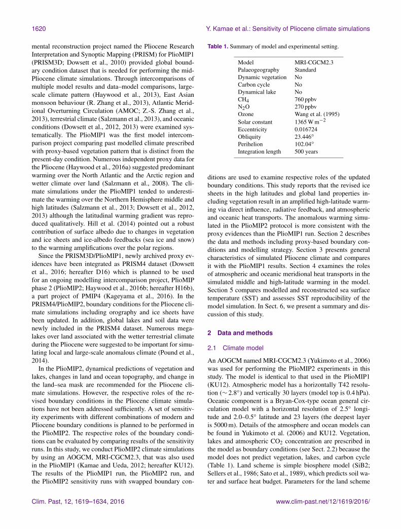
To simulate the Pliocene climate, the PRISM4 globalpalaeoenvironmental dataset (D16) including atmospherictrace gases, orography, vegetation covers, ice sheets, andlakes are prescribed in the model. Pliocene orography wasupdated from the PRISM3D (Sohl et al., 2009) by consid-ering mantle flow (Rowley et al., 2013) and glacial iso-static response of ice sheet loading (Raymo et al., 2011).We added anomalous orography (Pliocene minus modern)

Modern(a)

Pliocene(b)

90° N

60° N

30° N

EQ

30° S

60° S

90° S180° 120° W 60° W 0° 60° E 120° E 180°

90° N

60° N

30° N

EQ

30° S

60° S

90° S

Evergreen broadleafDeciduous broadleaf + evergreen coniferEvergreen coniferDeciduous coniferGrass land + deciduous conifer

Grass landSemi-desertTundraDesertLand ice

0709101113

0103040506

180° 120° W 60° W 0° 60° E 120° E 180°

Figure 1. Prescribed land cover (SiB2 classification) for (a) modernand (b) Pliocene conditions.

to the model’s modern orography (Fig. 3) according to the“anomaly method” recommended in the PlioMIP2 (H16b).Direct proxy evidences for the Greenland and Antarctic icesheets during the Pliocene were not available. The PRISM4provided Greenland ice sheet data that are confined to highelevations in the East Greenland Mountains suggested byresults of Pliocene Land Ice Sheet Model IntercomparisonProject (Dolan et al., 2015; Koenig et al., 2015). Accord-ing to proxy data for the Antarctic ice sheet (Naish et al.,2009; Pollard and DeConto, 2009), ice-free condition andthe identical ice sheet estimate to the PRISM3D were as-sumed in the West and East Antarctica, respectively (D16;Figs. 1b, 3). The resultant prescribed ice sheets over theGreenland and Antarctica are smaller than that in KU12. Weprescribed the Pliocene ice sheets by changing land orogra-phy (Fig. 3) and land cover (Fig. 1) over the ice sheets re-gions. Because the model does not predict dynamic vegeta-tion, we prescribe vegetation pattern (Fig. 1b) that is identicalto the PRISM3D/PlioMIP1 (Salzmann et al., 2008), accord-ing to the recommendation in H16b.

In addition to vegetation, global lake distribution dur-ing the Pliocene was also suggested to be distinct fromthe present day. Schuster et al. (2001, 2006) and Grif-

www.clim-past.net/12/1619/2016/ Clim. Past, 12, 1619–1634, 2016


Table 2. Details of six PlioMIP2 experiments examined in this study. PlioMIP1 Pliocene run represents AOGCM_NFA run in Kamae andUeda (2012). Soil and land–sea mask are identical among all the experiments.

Experiments Orography, lakes Vegetation Ice sheet CO2(ppmv)

E280 (Pre-industrial) Modern Modern Modern 280E400 Modern Modern Modern 400E560 Modern Modern Modern 560Ei280 Modern Modern Pliocene 280Eo280 Pliocene Pliocene Modern 280Eoi400 (Pliocene) Pliocene Pliocene Pliocene 400PlioMIP1 Pliocene PlioMIP1 orography, Pliocene PlioMIP1 405

modern lake

Table 3. Anomalies in global-mean surface air temperature (1SAT;◦C) in the PlioMIP2 runs relative to E280. The anomalies are cal-culated by averages for the last 50 years of the individual runs.

Experiments Global-mean1SAT (◦C)

E400 1.7E560 2.8Ei280 0.3Eo280 0.5Eoi400 2.4PlioMIP1 1.8

fin (2006) suggested the existence of the African Megalakesexisted during the Miocene and the Pliocene. Contoux etal. (2013) and Pound et al. (2014) pointed out an impor-tant role of the Pliocene lakes in the global climate throughlocal atmosphere–land interaction and remote influences.The PRISM4 provides global lake area data (Pound et al.,2014) for the PlioMIP2 (Fig. 2). We prescribe the Pliocenelakes (Fig. 2b; Table 2) by adding anomalous areas of lakes(Fig. 2c) to model’s modern lakes (the Caspian Sea, the AralSea, Lake Balkhash, Lake Chad and Lake Eyre; Fig. 2a).

In this paper, the results of six PlioMIP2 experiments(Table 2) are reported: pre-industrial run; Pliocene run;pre-industrial runs but with CO2 concentration of 400 and560 ppmv (hereafter E400 and E560 runs); pre-industrial runbut with Pliocene ice sheets (Ei280 run); and pre-industrialrun but with Pliocene orography, vegetation, and lakes (OVL)except over the ice sheet regions (hereafter Eo280 run). CH4,N2O, ozone, solar constant, orbital parameters are identicalto the pre-industrial run (Table 1). Land orography, lake area,vegetation, land ice, atmospheric CO2 concentration are al-tered in the Pliocene run from the pre-industrial run. Combi-nations of the boundary conditions are changed in the sen-sitivity runs so that the impacts of the individual compo-nents can be evaluated (Table 2; Sect. 2.3). A large spreadremains in the assessment of the Pliocene CO2 concentration(e.g. Raymo et al., 1996; Seki et al., 2010; D16). Although

400 ppmv of CO2 concentration is prescribed in the Pliocenerun, other concentrations are also used in the other sensitivityruns (H16b). In this paper, we examine the results of simu-lations with CO2 concentration of 280, 400, and 560 ppmv(Table 2).

The results are also compared with PlioMIP1 run con-ducted in KU12 (Table 2). Pliocene lakes were set to beidentical to the modern. The PRISM3D-based vegetation(Salzmann et al., 2008) was also prescribed in the PlioMIP1Pliocene run (Fig. 1b). A prescribed CO2 concentration of405 ppmv was slightly higher than the PlioMIP2.

The initial condition for the PlioMIP2 runs is identical tothe pre-industrial run: 31 December of the PlioMIP1 controlrun (in NFA_AOGCM) after 500-year spin up (Fig. 3b inKU12). The model is integrated for another 500 years withswapped boundary conditions and the last 50 years are usedfor analyses. Note that reconstructed deep ocean temperaturewas added to the initial condition of the PlioMIP1 Pliocenerun (KU12), distinct to the PlioMIP2. Despite the differencein the initial deep ocean temperature, ocean circulation andSST after the 500-year integrations are generally similar be-tween the two (see Sects. 3.3, 4, 5).

2.3 Respective roles of boundary conditions

In the PlioMIP2, relative contributions of the boundary con-ditions to climate anomalies (e.g. global mean warming) canbe evaluated by comparing the set of sensitivity experiments(H16b). In this study, we use the six PlioMIP2 simulations(Table 2) and evaluate the respective contributions by fol-lowing Eqs. (1)–(6):

All = [Eoi400]− [E280], (1)CO2 = [E400]− [E280], (2)OVL = [Eo280]− [E280], (3)

Ice Sheet = [Ei280]− [E280], (4)Sum = CO2 +OVL + IceSheet, (5)

Residual = All-Sum, (6)



Lake area Modern(a)

Lake area Pliocene(b)

90° N

60° N

30° N

EQ

30° S

60° S

90° S

90° N

60° N

30° N

EQ

30° S

60° S

90° S

180° 120° W 60° E 0° 60° E 120° E 180°

0.1 0.3 0.5 0.7 0.8 0.9

Lake area Pliocene–Modern(c)90° N

60° N

30 °N

EQ

30° S

60° S

90° S

0.01 0.2 0.4 0.6 0.8 0.9

180° 120° W 60° E 0° 60° E 120° E 180°

180° 120° W 60° E 0° 60° E 120° E 180°

Figure 2. Prescribed lake area fraction over land. (a) Modern,(b) Pliocene, and (c) Pliocene minus modern.

where [] represents the experiment name (Table 2). E280 andEoi400 indicate the pre-industrial and Pliocene runs, respec-tively. Difference of results between Eo280 and E280 runcorresponds to effect of differences in OVL. Sum of Eqs. (2)–(4) is used as a reconstruction of Eq. (1). By Eqs. (5), (6),we can compare the simulated climate anomaly between thePliocene run and the pre-industrial and its reconstruction.Residual (Eq. 6) indicates a nonlinear effect of combinationof the boundary conditions associated with nonlinearity inforcing–response relationship (e.g. Shiogama et al., 2013).This decomposition method is not identical to that recom-mended in H16b. While decomposed relative contributionscould be dependent on the choice of quantifying methods,Residual term shown in this study is generally minor to All

m100 500 1000–100–500–1000 1500 2000–1500–2000

Orography Pliocene–Modern90° N

60° N

30° N

EQ

30° S

60° S

90° S180° 120° W 60° W 0° 60° E 120° E 180°

Figure 3. Prescribed anomaly in land orography (m) for Pliocenerelative to modern.

Eoi400Ei280E400

Eo280

E280

3002001000 500400

14

15

16

13

12

SAT

(°C

)

Time (year)

E560

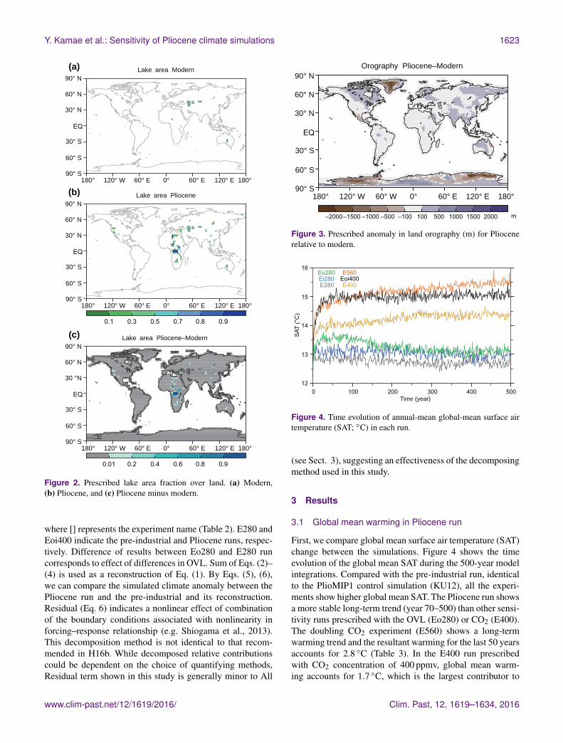
Figure 4. Time evolution of annual-mean global-mean surface airtemperature (SAT; ◦C) in each run.

(see Sect. 3), suggesting an effectiveness of the decomposingmethod used in this study.

3 Results

3.1 Global mean warming in Pliocene run

First, we compare global mean surface air temperature (SAT)change between the simulations. Figure 4 shows the timeevolution of the global mean SAT during the 500-year modelintegrations. Compared with the pre-industrial run, identicalto the PlioMIP1 control simulation (KU12), all the experi-ments show higher global mean SAT. The Pliocene run showsa more stable long-term trend (year 70–500) than other sensi-tivity runs prescribed with the OVL (Eo280) or CO2 (E400).The doubling CO2 experiment (E560) shows a long-termwarming trend and the resultant warming for the last 50 yearsaccounts for 2.8 ◦C (Table 3). In the E400 run prescribedwith CO2 concentration of 400 ppmv, global mean warm-ing accounts for 1.7 ◦C, which is the largest contributor to



All(a) CO(b)

Orog + Veg + Lake (OVL)(c) Ice sheet(d)

SAT (°C)

90° N

60° N

30° N

EQ

30° S

60° S

90° S

90° N

60° N

30° N

EQ

30° S

60° S

90° S

90°N

60°N

30°N

EQ

30°S

60°S

90°S

90°N

60°N

30°N

EQ

30°S

60°S

90°S

0 1 2–1–2 3–3 4 5 6 7 8 10

All(e) CO(f)

OVL(g) Ice sheet(h)

SST (°C)

90° N

60° N

30°N

EQ

30° S

60° S

90° S

90° N

60° N

30° N

EQ

30° S

60° S

90° S

90°N

60°N

30°N

EQ

30°S

60°S

90°S

90°N

60°N

30°N

EQ

30°S

60°S

90°S

0 1 2–1–2 3–3

2

2

180° 120° W 60° W 0° 60° E 120° E 180° 180° 120° W 60° W 0° 60° E 120° E 180°

180° 120° W 60° W 0° 60° E 120° E 180° 180° 120° W 60° W 0° 60° E 120° E 180°

180° 120° W 60° W 0° 60° E 120° E 180° 180° 120° W 60° W 0° 60° E 120° E 180°

180° 120° W 60° W 0° 60° E 120° E 180° 180° 120° W 60° W 0° 60° E 120° E 180°

Figure 5. (a) Anomaly in SAT (◦C) in Pliocene run relative to pre-industrial run (hereafter All). (b) E400 run minus pre-industrial run(CO2), (c) Eo280 run minus pre-industrial run (OVL), and (d) Ei280 run minus pre-industrial run (Ice Sheet), respectively. The anomaliesare calculated by averages for the last 50 years of the individual runs. (e–h) Similar to (a–d), but for sea surface temperature (SST; ◦C).Intervals of grey contours are 1.5 ◦C.

the Pliocene warmth among the boundary conditions (68 %;Table 3), consistent with Willeit et al. (2013). Here Sum(2.5 ◦C) can reconstruct All (2.4 ◦C) quantitatively. Contri-butions of Ice Sheet and OVL are 12 and 20 %, respectively.

Compared with the PlioMIP1 run (1.8 ◦C), the PlioMIP2Pliocene run shows a larger warming (+39 %, 0.7 ◦C) al-though the prescribed CO2 concentration (400 ppmv) isslightly lower (405 ppmv in PlioMIP1). In the next section,



we compare spatial patterns of the results and decompose re-spective contributions of the individual boundary conditions.

3.2 Regional changes in temperature and precipitation

Figure 5 shows spatial distributions of annual mean SATanomalies averaged over the last 50 years. Similar to thePlioMIP1 run (KU12; Haywood et al., 2013), the Plioceneanomaly exhibits a polar amplification of surface warming(i.e. warming peaks over the high latitudes including Green-land and the Antarctica). While land surface warming is gen-erally larger than the ocean surface warming (in responseto CO2 forcing; Fig. 5b; Manabe et al., 1991; Kamae etal., 2014), regional differences in SAT change (weak warm-ing compared with surrounding areas) are found over south-ern North America, tropical Africa, Indian subcontinent, andeastern Siberia, similar to the PlioMIP1 (KU12). Zonally av-eraged SAT change exhibits (1) minimum warming over theSouthern Hemisphere middle latitude; (2) moderate warmingover the tropics; and (3) warming peaks over the Southernand Northern Hemisphere high latitudes (Fig. 6a). SST alsoexhibits the inter-hemispheric warming asymmetry (Figs. 5e,6b; see Sect. 3.3) and warming peak in the Northern Hemi-sphere mid-to-high-latitude (particularly in the eastern NorthPacific and North Atlantic; Figs. 5e, 6b). Here Sum of zonalmean SAT, SST and other variables (e.g. precipitation) aresimilar to All (Fig. 6), indicating a limited Residual term inthe zonal mean (Eq. 6). The effectiveness of reconstructionof All by Sum suggests that characteristics of the Plioceneclimate anomaly can be decomposed into the individual con-tributions by Eq. (5). Note that Sum tends to underestimate(overestimate) the Southern (Northern) Hemisphere middleand high-latitude warming, suggesting an importance of non-linear effects (see Sect. 4).

Compared to the PlioMIP1, the Pliocene run exhibits alarger warming over Antarctica and the Northern Hemi-sphere middle and high latitudes (Fig. 6a), resulting in thelarger increase in global mean SAT (Sect. 3.1). In additionto the less ice sheets over Greenland and West Antarctica,other factors also contribute to the polar amplification ofsurface warming (Figs. 5, 6a). The decomposition based onthe sensitivity runs (Sect. 2.3) indicates that all the bound-ary conditions contribute to the polar warming (Figs. 5, 6a).Contributions of OVL and CO2 to the zonal mean polarwarming are dominant (Figs. 5b, c, 6a). Here OVL is thelargest contributor to the latitudinal difference in the North-ern Hemisphere warming and the inter-hemispheric warm-ing contrast (Fig. 6a). Although spatially smooth CO2 ra-diative forcing also leads to the polar amplification (Fig. 6a;e.g. Serreze and Barry, 2011; Hill et al., 2014), OVL effectdominates the meridional warming contrast. Note that CO2 isthe largest contributor to the global mean Pliocene warming(Sect. 3.1). In Sect. 5, we assess reproducibility of the SSTin the PlioMIP2 and 1 runs by comparing with proxy-basedestimate.

(a)90° N

60° N

30° N

EQ

30° S

60° S

90° S

SAT SST Pr MMC

10–2 10–2 1.2–0.4 6–6(°C) (°C) (mm day )–1

(b) (c) (d)

2 6 2 6 0.4

Albedo SIC

0.3–0.3 50–50(%)

(e) (f)

0 0

90° N

60° N

30° N

EQ

30° S

60° S

90° S

Atm NHT Atl NHT

0.4–0.6(PW)

(g) (h)

0

All

Ice sheet

CO2OVL

SumPlioMIP1

E280/2

(10 kg s )–110 0

0.4–0.6(PW)

0

Figure 6. Zonal-mean anomalies in (a) SAT (◦C), (b) SST (◦C),(c) precipitation (mm day−1), (d) mass stream function of meanmeridional circulation at 500 hPa level (1010 kg s−1), (e) surfacealbedo, (f) sea ice concentration (%), (g) northward heat transportdue to atmosphere (PW) and (h) the Atlantic (PW). Black, yellow,green, and blue lines represent All, CO2, OVL, and Ice Sheet, re-spectively. Grey line represents Sum. Dashed red lines representresults of AOGCM_NFA run conducted in the identical model inPlioMIP1 (Kamae and Ueda, 2012). Dotted grey line in (d) repre-sents climatology in pre-industrial run multiplied by 0.5.

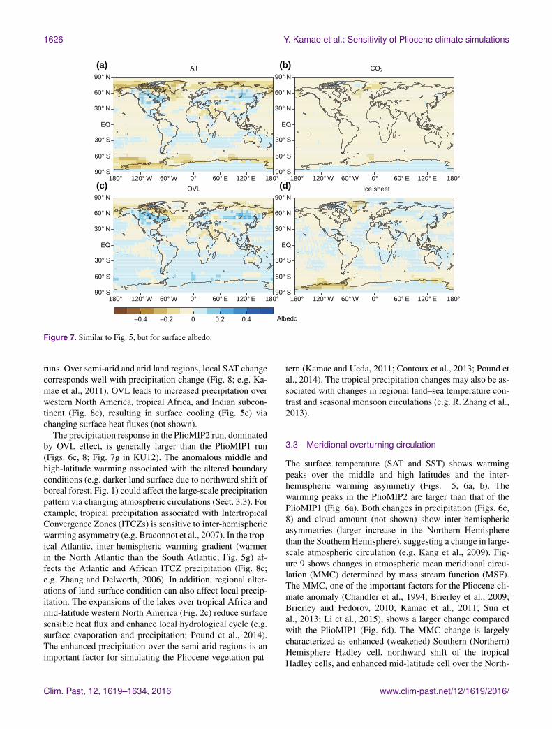
Figures 7 and 6e show change in surface albedo and itszonal mean. Increasing albedo over North America middlelatitude and eastern Siberia due to change in vegetation (bo-real forest in modern but grassland in the Pliocene; Fig. 1;Haywood et al., 2013; Hill et al., 2014), a part of OVL ef-fect, contributes to the regional difference in the SAT change(Figs. 5c, 7c). Over the Northern Hemisphere high latitude,the reduced ice sheets (Figs. 1, 3) and a reduction of surfacealbedo (Figs. 6e, 7c) due to northward shift of boreal forest(deciduous conifer, tundra and bare soil regions over northernCanada and northeastern Eurasia; Fig. 1) result in regionalwarming (Fig. 5c, d). Surface snow cover (not shown) alsoaffects partly the land surface albedo. The high-latitude SATis more sensitive to imposed albedo change due to the al-tered vegetation cover (Fig. 1) than low latitude (Davin andde Noblet-Ducoudré, 2010), consistent with the substantialArctic warming found in the current study (Fig. 5) and previ-ous studies (Willeit et al., 2013; Zhang and Jiang, 2014). De-creasing albedo over the high-latitude ocean (the Arctic andAntarctic Ocean) corresponds to sea ice reductions (Fig. 6e,f) that are larger than the PlioMIP1 (Fig. 6f; Howell et al.,2016). Sea ice and snow albedo feedback contributes to thedifferential polar and global-mean warming between the two



All(a) CO2(b)

OVL(c) Ice sheet(d)

Albedo

90° N

60° N

30° N

EQ

30° S

60° S

90° S

90° N

60° N

30° N

EQ

30° S

60° S

90° S

90° N

60° N

30° N

EQ

30° S

60° S

90° S

90° N

60° N

30° N

EQ

30° S

60° S

90° S180° 120° W 60° W 0° 60° E 120° E 180° 180° 120° W 60° W 0° 60° E 120° E 180°

180° 120° W 60° W 0° 60° E 120° E 180° 180° 120° W 60° W 0° 60° E 120° E 180°

0 0.2 0.4–0.2–0.4

Figure 7. Similar to Fig. 5, but for surface albedo.

runs. Over semi-arid and arid land regions, local SAT changecorresponds well with precipitation change (Fig. 8; e.g. Ka-mae et al., 2011). OVL leads to increased precipitation overwestern North America, tropical Africa, and Indian subcon-tinent (Fig. 8c), resulting in surface cooling (Fig. 5c) viachanging surface heat fluxes (not shown).

The precipitation response in the PlioMIP2 run, dominatedby OVL effect, is generally larger than the PlioMIP1 run(Figs. 6c, 8; Fig. 7g in KU12). The anomalous middle andhigh-latitude warming associated with the altered boundaryconditions (e.g. darker land surface due to northward shift ofboreal forest; Fig. 1) could affect the large-scale precipitationpattern via changing atmospheric circulations (Sect. 3.3). Forexample, tropical precipitation associated with IntertropicalConvergence Zones (ITCZs) is sensitive to inter-hemisphericwarming asymmetry (e.g. Braconnot et al., 2007). In the trop-ical Atlantic, inter-hemispheric warming gradient (warmerin the North Atlantic than the South Atlantic; Fig. 5g) af-fects the Atlantic and African ITCZ precipitation (Fig. 8c;e.g. Zhang and Delworth, 2006). In addition, regional alter-ations of land surface condition can also affect local precip-itation. The expansions of the lakes over tropical Africa andmid-latitude western North America (Fig. 2c) reduce surfacesensible heat flux and enhance local hydrological cycle (e.g.surface evaporation and precipitation; Pound et al., 2014).The enhanced precipitation over the semi-arid regions is animportant factor for simulating the Pliocene vegetation pat-

tern (Kamae and Ueda, 2011; Contoux et al., 2013; Pound etal., 2014). The tropical precipitation changes may also be as-sociated with changes in regional land–sea temperature con-trast and seasonal monsoon circulations (e.g. R. Zhang et al.,2013).

3.3 Meridional overturning circulation

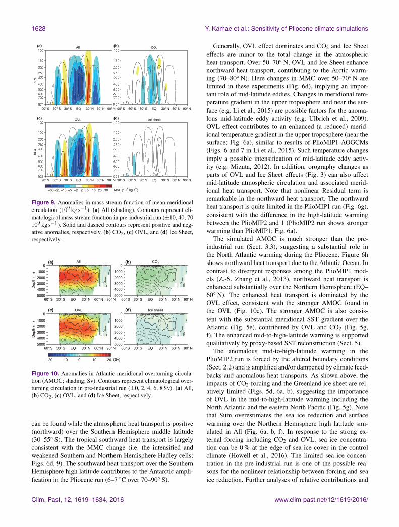
The surface temperature (SAT and SST) shows warmingpeaks over the middle and high latitudes and the inter-hemispheric warming asymmetry (Figs. 5, 6a, b). Thewarming peaks in the PlioMIP2 are larger than that of thePlioMIP1 (Fig. 6a). Both changes in precipitation (Figs. 6c,8) and cloud amount (not shown) show inter-hemisphericasymmetries (larger increase in the Northern Hemispherethan the Southern Hemisphere), suggesting a change in large-scale atmospheric circulation (e.g. Kang et al., 2009). Fig-ure 9 shows changes in atmospheric mean meridional circu-lation (MMC) determined by mass stream function (MSF).The MMC, one of the important factors for the Pliocene cli-mate anomaly (Chandler et al., 1994; Brierley et al., 2009;Brierley and Fedorov, 2010; Kamae et al., 2011; Sun etal., 2013; Li et al., 2015), shows a larger change comparedwith the PlioMIP1 (Fig. 6d). The MMC change is largelycharacterized as enhanced (weakened) Southern (Northern)Hemisphere Hadley cell, northward shift of the tropicalHadley cells, and enhanced mid-latitude cell over the North-



All(a) CO2(b)

OVL(c) Ice sheet(d)

Pr (mm day )

90° N

60° N

30° N

EQ

30° S

60° S

90° S

90° N

60° N

30° N

EQ

30° S

60° S

90° S

90° N

60° N

30° N

EQ

30° S

60° S

90° S

90° N

60° N

30° N

EQ

30° S

60° S

90° S180° 120° W 60° W 0° 60° E 120° E 180° 180° 120° W 60° W 0° 60° E 120° E 180°

180° 120° W 60° W 0° 60° E 120° E 180° 180° 120° W 60° W 0° 60° E 120° E 180°

–0.4–1–2 0.4 1 2 4–4–1

Figure 8. Similar to Fig. 5, but for precipitation (mm day−1).

ern Hemisphere (Figs. 6d, 9a). The boundary of the twoHadley cells and northern edge of the northern cell (deter-mined by signs of MSF at 500 hPa level; Fig. 6d) shift north-ward for 7.2 and 2.0◦, respectively, and the mid-latitude cellis enhanced for 41 %, largely according to the OVL effect(Figs. 6d, 9c). The change in the Hadley circulation is consis-tent with the PlioMIP1 qualitatively but larger quantitatively,suggesting an anomalous meridional heat transport due to theMMC (see Sect. 4).

The simulated SST anomaly shows the remarkable merid-ional warming gradient, particularly over the Atlantic(Fig. 5), resulting from a substantial anomaly in the AMOC.Climatological AMOC in the pre-industrial run shown inFig. 10 (4.2 Sv) is weaker than observations (e.g. Buck-ley and Marchall, 2016) and other PlioMIP1 models (Z.-S. Zhang et al., 2013). Note that AMOC simulated in MRI-CGCM2.3 shown in Z.-S. Zhang et al. (2013) is a result ofsimulation with the flux adjustments (KU12). The PlioceneAMOC simulated in the PlioMIP2 (without any flux adjust-ments) is quite stronger (+15 Sv) than the pre-industrial run,suggesting an intensified northward heat transport due to theAtlantic. The AMOC change dominates in OVL (+14.5 Sv;Fig. 10c) and enhancement due to CO2 is moderate. Herechange in sea surface density flux over the North Atlantic(Speer and Tziperman, 1992) is one of possible controllingfactors for the OVL-induced AMOC change. In response tothe prescribed boundary conditions, changes in air and sur-

face water temperature, atmospheric humidity, cloud cover,and surface wind speed can influence on sea surface heatfluxes (sensible heat flux, latent heat flux, and longwave andshortwave radiative flux). In addition, changes in river runoff,sea ice melt, and precipitation minus evaporation can affectsea surface salinity. These heat and salinity fluxes possiblymodulate AMOC strength in the Pliocene climate. We plan toaddress physical processes contributing to the OVL-inducedstronger AMOC in a separated paper. In the next section, wediscuss possible factors contributing to the substantial higherlatitude warming found in the Pliocene run.

4 Mid- and high-latitude warming and meridionalheat transport

The PlioMIP2 run shows the larger middle and high-latitudewarming over the Northern Hemisphere (9 ◦C at 75◦ N;Fig. 6a) compared with the PlioMIP1 run. Hill et al. (2014)evaluated the contributions of factors for the polar amplifi-cation by using eight PlioMIP1 models. Despite substantialinter-model spreads, strong warming due to reduced surfacealbedo was robustly found in all the models and relative con-tribution of meridional heat transport (due to the atmosphereand ocean) was minor. Figure 6g shows anomalous north-ward heat transport due to the atmosphere. Over the South-ern Hemisphere high latitude and tropics to Northern Hemi-sphere middle latitude, anomalous southward heat transport



All(a) CO2(b)

OVL(c) Ice sheet(d)

90° S 60° S 30° S EQ 30° N 60° N 90° N

MSF (10 kg s )

90° S 60° S 30° S EQ 30° N 60° N 90° N

90° S 60° S 30° S EQ 30° N 60° N 90° N 90° S 60° S 30° S EQ 30° N 60° N 90° N

hPa

hPa

9 -12 5 10–2–5 20 30–10–20–30

Figure 9. Anomalies in mass stream function of mean meridionalcirculation (109 kg s−1). (a) All (shading). Contours represent cli-matological mass stream function in pre-industrial run (±10, 40, 70109 kg s−1). Solid and dashed contours represent positive and neg-ative anomalies, respectively. (b) CO2, (c) OVL, and (d) Ice Sheet,respectively.

60°S 30°S EQ 30°N 60°N 90°N

Dep

th (m

)

010002000300040005000

–20 0 20 (Sv)–10 10

60° S 30° S EQ 30° N 60° N 90° N

Dep

th (m

)

010002000300040005000

All CO2

OVL Ice sheet

(a)

(c)

(b)

(d)

60°S 30°S EQ 30°N 60°N 90°N

010002000300040005000

60° S 30° S EQ 30° N 60° N 90° N

010002000300040005000

Figure 10. Anomalies in Atlantic meridional overturning circula-tion (AMOC; shading; Sv). Contours represent climatological over-turning circulation in pre-industrial run (±0, 2, 4, 6, 8 Sv). (a) All,(b) CO2, (c) OVL, and (d) Ice Sheet, respectively.

can be found while the atmospheric heat transport is positive(northward) over the Southern Hemisphere middle latitude(30–55◦ S). The tropical southward heat transport is largelyconsistent with the MMC change (i.e. the intensified andweakened Southern and Northern Hemisphere Hadley cells;Figs. 6d, 9). The southward heat transport over the SouthernHemisphere high latitude contributes to the Antarctic ampli-fication in the Pliocene run (6–7 ◦C over 70–90◦ S).

Generally, OVL effect dominates and CO2 and Ice Sheeteffects are minor to the total change in the atmosphericheat transport. Over 50–70◦ N, OVL and Ice Sheet enhancenorthward heat transport, contributing to the Arctic warm-ing (70–80◦ N). Here changes in MMC over 50–70◦ N arelimited in these experiments (Fig. 6d), implying an impor-tant role of mid-latitude eddies. Changes in meridional tem-perature gradient in the upper troposphere and near the sur-face (e.g. Li et al., 2015) are possible factors for the anoma-lous mid-latitude eddy activity (e.g. Ulbrich et al., 2009).OVL effect contributes to an enhanced (a reduced) merid-ional temperature gradient in the upper troposphere (near thesurface; Fig. 6a), similar to results of PlioMIP1 AOGCMs(Figs. 6 and 7 in Li et al., 2015). Such temperature changesimply a possible intensification of mid-latitude eddy activ-ity (e.g. Mizuta, 2012). In addition, orography changes asparts of OVL and Ice Sheet effects (Fig. 3) can also affectmid-latitude atmospheric circulation and associated merid-ional heat transport. Note that nonlinear Residual term isremarkable in the northward heat transport. The northwardheat transport is quite limited in the PlioMIP1 run (Fig. 6g),consistent with the difference in the high-latitude warmingbetween the PlioMIP2 and 1 (PlioMIP2 run shows strongerwarming than PlioMIP1; Fig. 6a).

The simulated AMOC is much stronger than the pre-industrial run (Sect. 3.3), suggesting a substantial role inthe North Atlantic warming during the Pliocene. Figure 6hshows northward heat transport due to the Atlantic Ocean. Incontrast to divergent responses among the PlioMIP1 mod-els (Z.-S. Zhang et al., 2013), northward heat transport isenhanced substantially over the Northern Hemisphere (EQ–60◦ N). The enhanced heat transport is dominated by theOVL effect, consistent with the stronger AMOC found inthe OVL (Fig. 10c). The stronger AMOC is also consis-tent with the substantial meridional SST gradient over theAtlantic (Fig. 5e), contributed by OVL and CO2 (Fig. 5g,f). The enhanced mid-to-high-latitude warming is supportedqualitatively by proxy-based SST reconstruction (Sect. 5).

The anomalous mid-to-high-latitude warming in thePlioMIP2 run is forced by the altered boundary conditions(Sect. 2.2) and is amplified and/or dampened by climate feed-backs and anomalous heat transports. As shown above, theimpacts of CO2 forcing and the Greenland ice sheet are rel-atively limited (Figs. 5d, 6a, b), suggesting the importanceof OVL in the mid-to-high-latitude warming including theNorth Atlantic and the eastern North Pacific (Fig. 5g). Notethat Sum overestimates the sea ice reduction and surfacewarming over the Northern Hemisphere high latitude sim-ulated in All (Fig. 6a, b, f). In response to the strong ex-ternal forcing including CO2 and OVL, sea ice concentra-tion can be 0 % at the edge of sea ice cover in the controlclimate (Howell et al., 2016). The limited sea ice concen-tration in the pre-industrial run is one of the possible rea-sons for the nonlinear relationship between forcing and seaice reduction. Further analyses of relative contributions and



inter-model consistency of cloud and surface albedo, long-wave radiation, meridional heat transport due to atmosphereand individual ocean basins by using PlioMIP2 multi-modelsmay contribute to improving the understanding of the physi-cal mechanisms responsible for the Pliocene polar amplifica-tion.

5 Data–model comparison of SST

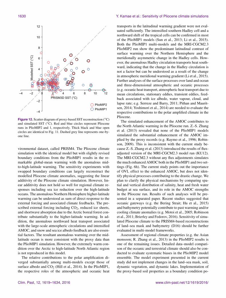
The Pliocene AMOC is apparently distinct from the pre-industrial run (Fig. 10), resulting in the anomalous northwardheat transport due to the Atlantic Ocean (Fig. 6h). Here thelarger North Atlantic warming (3–7 ◦C in 30–70◦ N; Fig. 5e)in the PlioMIP2 Pliocene run than the PlioMIP1 implies abetter reproducibility of the mid-to-high-latitude SST warm-ing that was robustly underestimated among the PlioMIP1multi-models (Dowsett et al., 2013). Figure 11 shows com-parison of simulated SST and PRISM3D proxy-based SSTreconstruction during the Pliocene (Dowsett et al., 2009).Note that the PRISM4 SST reconstruction is not updated(Dowsett et al., 2016) since PRISM3D. The SST reconstruc-tion is characterized as extremely high SST in the NorthAtlantic high latitude, low-to-mid-latitude warming gradient(limited change in the tropics and warming in the middle lat-itude, respectively), and remarkable warming in mid-latitudecoastal areas (off the west coast of North America and SouthAmerica, and off the east coast of the Eurasian Continent;Dowsett et al., 2009, 2013).

Figures 11 and 12 compare SST biases found in thePlioMIP2 and 1. Generally, both the PlioMIP2 and 1 tendto underestimate the mid-to-high-latitude warming suggestedby proxy records (blue circles in Fig. 11a; Haywood et al.,2013). However, the large part of underestimation of themid-to-high-latitude warming is reduced substantially in thePlioMIP2 run (green circles in Fig. 11b). In contrast to theremarkable underestimation (SST bias is larger than 4 ◦C;Fig. 12) of the mid-latitude warming (the North Atlantic, offthe west coast of North America and South America, andoff the east coast of the Eurasian Continent) in the PlioMIP1(black circles in Figs. 11 and 12), the SST biases are re-duced in the PlioMIP2 run (Figs. 11b and 12). From a zonal-mean perspective, the larger mid-to-high-latitude warming(Fig. 6a, b) in the PlioMIP2 run is more consistent with theproxy evidences than the PlioMIP1 (Figs. 11b, 12). Note thatSST bias (8.9–12 ◦C in 69–81◦ N) over the North Atlantichigh latitude (open blue circles in Figs. 11 and 12) is stillnot reduced in this simulation. This data–model discord wasalso consistently found in PlioMIP1 multiple climate models(Dowsett et al., 2013). Haywood et al. (2013) noted that thissubstantial data–model discord is highly dependent on meanannual temperature estimate based on geochemically basedproxy data and is not derived from faunal-based estimates ofcold–warm month means. They suggested that we should notrely on this data–model discord too much until more variety

SST bias PlioMIP2 – PRISM3D(a)90° N

60° N

30° N

EQ

30° S

60° S

90° S180° 120° W 60° W 0° 60° E 120° E 180°

SignConfidence

Negative PositiveMedium High Very high

°C0 1 2–1–2 3–3 4–4

°C0 1 2–1–2 3–3 4–4

SST bias PlioMIP2 – PlioMIP1(b)90° N

60° N

30° N

EQ

30° S

60° S

90° S180° 120° W 60° W 0° 60° E 120° E 180°

Smaller bias Larger bias

Figure 11. (a) SST bias (◦C) in PlioMIP2 Pliocene run comparedwith PRISM3D proxy-based SST reconstruction (Dowsett et al.,2009). Coloured circles and triangles represent cool and warm bi-ases, respectively. Sizes of plots indicate confidence levels of SSTestimate based on chronology, sampling density, sampling qual-ity and performance of quantitative method (Dowsett et al., 2013).Thick black and blue open circles indicate proxy sites in which es-timated SST anomalies are large (between 4.0 and 8.9 ◦C) and ex-tremely large (> 8.9 ◦C), respectively. (b) Comparison of SST biasesin Pliocene runs between PlioMIP2 and 1. Coloured plots indicatedifferences in absolute biases between the two.

of proxy records is available from more locations in the high-latitude North Atlantic. In addition to the possible issue onthe proxy-based estimate, modelled biases in AMOC and/orsea ice can also contribute to the North Atlantic data–modeldiscord.

6 Summary and discussion

The PlioMIP2 simulations are conducted by using MRI-CGCM2.3 and prescribing the updated Pliocene palaeoen-



PRISM3D SST (°C)0 2–2 4–4 6 8 10 12

–4

–2

0

2

4

6

8

10

12

PlioMIP2PlioMIP1

Mod

elle

d SS

T (°

C)

Figure 12. Scatter diagram of proxy-based SST reconstruction (◦C)and simulated SST (◦C). Red and blue circles represent Plioceneruns in PlioMIP2 and 1, respectively. Thick black and blue opencircles are identical to Fig. 11. Dashed grey line represents one-by-one line.

vironmental dataset, called PRISM4. The Pliocene climatesimulation with the identical model but with slightly revisedboundary conditions from the PlioMIP1 results in the re-markable global-mean warming with the anomalous mid-to-high-latitude warming. The sensitivity experiments withswapped boundary conditions can largely reconstruct themodelled Pliocene climate anomalies, suggesting the linearadditivity of the Pliocene climate simulation. However, lin-ear additivity does not hold so well for regional climate re-sponses including sea ice reduction over the high-latitudeoceans. The anomalous Northern Hemisphere higher-latitudewarming can be understood as sum of direct response to theexternal forcing and associated climate feedbacks. The pre-scribed external forcing including CO2, reduced ice sheets,and shortwave absorption due to the Arctic boreal forest con-tribute substantially to the higher-latitude warming. In ad-dition, the anomalous northward heat transport associatedwith the large-scale atmospheric circulations and intensifiedAMOC, and snow and sea ice albedo feedback are also essen-tial factors. The resultant anomalous warming over the mid-latitude ocean is more consistent with the proxy data thanthe PlioMIP1 simulation. However, the extremely warm con-dition over the Arctic to high-latitude North Atlantic regionis not reproduced in this model.

The relative contributions to the polar amplification di-verged substantially among multi-models except those ofsurface albedo and CO2 (Hill et al., 2014). In the PlioMIP1,the respective roles of the atmospheric and oceanic heat

transports in the latitudinal warming gradient were not eval-uated sufficiently. The intensified southern Hadley cell and anorthward shift of the tropical cells can be confirmed in mostof the PlioMIP1 models (Sun et al., 2013; Li et al., 2015).Both the PlioMIP1 multi-models and the MRI-CGCM2.3PlioMIP2 run show the predominant latitudinal contrast ofsurface warming over the Northern Hemisphere and themeridionally asymmetric change in the Hadley cells. How-ever, the anomalous Hadley circulation transports heat south-ward, indicating that the change in the Hadley circulation isnot a factor but can be understood as a result of the changein atmospheric meridional warming gradient (Li et al., 2015).Further analyses of the surface processes over land and oceanand three-dimensional atmospheric and oceanic processes(e.g. oceanic heat transport, atmospheric heat transport due tomean circulations, stationary eddies, transient eddies, feed-back associated with ice albedo, water vapour, cloud, andlapse rate; e.g. Serreze and Barry, 2011; Pithan and Maurit-sen, 2014; Yoshimori et al., 2014) are needed to evaluate therespective contributions to the polar amplified climate in thePliocene.

The simulated enhancement of the AMOC contributes tothe North Atlantic warming in the Pliocene run. Z.-S. Zhanget al. (2013) revealed that none of the PlioMIP1 modelssimulated the substantial enhancement of the AMOC im-plied by the proxy records (e.g. Raymo et al., 1996; Robin-son, 2009). This is inconsistent with the current study be-cause Z.-S. Zhang et al. (2013) introduced the results of flux-adjusted version of the MRI-CGCM2.3 model run (KU12).The MRI-CGCM2.3 without any flux adjustments simulatesthe much enhanced AMOC both in the PlioMIP1 and two set-tings (Fig. 6h). The current study points out the importanceof OVL effect to the enhanced AMOC, but does not iden-tify physical processes contributing to the drastic change. Weplan to clarify the physical mechanisms by comparing spa-tial and vertical distribution of salinity, heat and fresh waterbudget at sea surface, and its role in the AMOC strengthsin the Pliocene run. Results of such analyses will be pre-sented in a separated paper. Recent studies suggested thatoceanic gateways (e.g. the Bering Strait; Hu et al., 2015)and bathymetry potentially contribute to past warming and/orcooling climate anomalies (e.g. Motoi et al., 2005; Robinsonet al., 2011; Brierley and Fedorov, 2016). Sensitivity of simu-lated Pliocene climate to the PRISM4-based reconstructionsof land–sea mask and bathymetry (D16) should be furtherevaluated in multi-model frameworks.

Assessment of regional climate properties (e.g. the Asianmonsoon; R. Zhang et al., 2013) in the PlioMIP2 results isone of the remaining issues. Detailed data–model compari-son of the oceanic and terrestrial climate should also be con-ducted to evaluate systematic biases in the PlioMIP2 modelensemble. The model experiment presented in the currentstudy did not implement changes in the land–sea mask, soil,dynamic vegetation, and dynamic lakes. Implementation ofthe proxy-based soil properties as a boundary condition po-



tentially affects the simulated Pliocene climate via changingsurface and atmospheric energy and water budget (Pound etal., 2014). Low-resolution models are not suitable for simu-lating the regional atmospheric circulation and hydrologicalcycle associated with land orography (e.g. Xie et al., 2006).We plan to conduct more complex PlioMIP2 simulations thatare more consistent with the proxy-based reconstructions byincorporating all the requested boundary conditions to anEarth system model or a high resolution AOGCM. Furthercomplex and fine resolution modelling, multiple model in-tercomparison, and data–model comparisons could advanceunderstanding of the factors for the Pliocene warming cli-mate.

7 Data availability

All the PlioMIP2/PRISM4 boundary condition data are avail-able from the USGS PlioMIP2 web page: http://geology.er.usgs.gov/egpsc/prism/7.2_pliomip2_data.html.

Acknowledgements. We thank anonymous reviewers for givingconstructive comments. The authors acknowledge PRISM4 andPRISM3D project members for archiving and providing globalpalaeoenvironmental datasets for the Pliocene climate modelsimulations. We also thank A. M. Haywood and A. M. Dolan forcoordinating the model intercomparison project, PlioMIP2.

Edited by: A. HaywoodReviewed by: two anonymous referees

References

Bellenger, H., Guilyardi, E., Leloup, J., Lengaigne, M., and Vialard,J.: ENSO representation in climate models: from CMIP3 toCMIP5, Clim. Dynam., 42, 1999–2018, 2014.

Braconnot, P., Otto-Bliesner, B., Harrison, S., Joussaume, S., Pe-terchmitt, J.-Y., Abe-Ouchi, A., Crucifix, M., Driesschaert, E.,Fichefet, Th., Hewitt, C. D., Kageyama, M., Kitoh, A., Loutre,M.-F., Marti, O., Merkel, U., Ramstein, G., Valdes, P., Weber,L., Yu, Y., and Zhao, Y.: Results of PMIP2 coupled simula-tions of the Mid-Holocene and Last Glacial Maximum – Part2: feedbacks with emphasis on the location of the ITCZ andmid- and high latitudes heat budget, Clim. Past, 3, 279–296,doi:10.5194/cp-3-279-2007, 2007.

Braconnot, P., Harrison, S. P., Kageyama, M., Bartlein, P. J.,Masson-Delmotte, V., Abe-Ouchi, A., Otto-Bliesner, B., andZhao, Y.: Evaluation of climate models using palaeoclimaticdata, Nature Climate Change, 2, 417–424, 2012.

Brierley, C. M. and Fedorov, A. V.: Relative importance of merid-ional and zonal sea surface temperature gradients for the onsetof the ice ages and Pliocene-Pleistocene climate evolution, Pale-oceanography, 25, PA2214, doi:10.1029/2009PA001809, 2010.

Brierley, C. M. and Fedorov, A. V.: Comparing the impacts ofMiocene–Pliocene changes in inter-ocean gateways on climate:Central American Seaway, Bering Strait, and Indonesia, EarthPlanet. Sc. Lett., 444, 116–130, 2016.

Brierley, C. M., Fedorov, A. V., Lui, Z., Herbert, T., Lawrence, K.,and LaRiviere, J. P.: Greatly expanded tropical warm pool andweakened Hadley circulation in the early Pliocene, Science, 323,1714–1718, 2009.

Buckley, M. W. and Marshall, J.: Observations, inferences, andmechanisms of the Atlantic Meridional Overturning Circulation:A review, Rev. Geophys., 54, 5–63, 2016.

Chandler, M. A., Rind, D., and Thompson, R. S.: Joint investiga-tions of the middle Pliocene climate II: GISS GCM NorthernHemisphere results, Global Planet. Change, 9, 197–219, 1994.

Contoux, C., Jost, A., Ramstein, G., Sepulchre, P., Krinner, G., andSchuster, M.: Megalake Chad impact on climate and vegetationduring the late Pliocene and the mid-Holocene, Clim. Past, 9,1417–1430, doi:10.5194/cp-9-1417-2013, 2013.

Davin, E. L. and de Noblet-Ducoudré, N.: Climatic impact ofglobal-scale deforestation: Radiative versus nonradiative pro-cesses, J. Climate, 23, 97–112, 2010.

Dolan, A. M., Hunter, S. J., Hill, D. J., Haywood, A. M., Koenig, S.J., Otto-Bliesner, B. L., Abe-Ouchi, A., Bragg, F., Chan, W.-L.,Chandler, M. A., Contoux, C., Jost, A., Kamae, Y., Lohmann, G.,Lunt, D. J., Ramstein, G., Rosenbloom, N. A., Sohl, L., Stepanek,C., Ueda, H., Yan, Q., and Zhang, Z.: Using results from thePlioMIP ensemble to investigate the Greenland Ice Sheet dur-ing the mid-Pliocene Warm Period, Clim. Past, 11, 403–424,doi:10.5194/cp-11-403-2015, 2015.

Dowsett, H. J., Cronin, T. M., Poore, R. Z., Thompson, R. S., What-ley, R. C., and Wood, A. M.: Micropaleontological evidence forincreased meridional heat transport in the North Atlantic Oceanduring the Pliocene, Science, 258, 1133–1135, 1992.

Dowsett, H. J., Robinson, M. M., and Foley, K. M.: Pliocene three-dimensional global ocean temperature reconstruction, Clim. Past,5, 769–783, doi:10.5194/cp-5-769-2009, 2009.

Dowsett, H. J., Robinson, M. M., Haywood, A. M., Salzmann, U.,Hill, D., Sohl, L., Chandler, M., Williams, M., Foley, K., andStoll, D. K.: The PRISM3D paleoenvironmental reconstruction,Stratigraphy, 7, 123–139, 2010.

Dowsett, H. J., Robinson, M. M., Haywood, A. M., Hill, D. J.,Dolan, A. M., Stoll, D. K., Chan, W.-L., Abe-Ouchi, A., Chan-dler, M. A., and Rosenbloom, N. A.: Assessing confidence inPliocene sea surface temperatures to evaluate predictive models,Nature Climate Change, 2, 365–371, 2012.

Dowsett, H. J., Foley, K. M., Stoll, D. K., Chandler, M. A., Sohl, L.E., Bentsen, M., Otto-Bliesner, B. L., Bragg, F. J., Chan, W.-L.,Contoux, C., Dolan, A. M., Haywood, A. M., Jonas, J. A., Jost,A., Kamae, Y., Lohmann, G., Lunt, D. J., Nisancioglu, K. H.,Abe-Ouchi, A., Ramstein, G., Riesselman, C. R., Robinson, M.M., Rosenbloom, N. A., Salzmann, U., Stepanek, C., Strother, S.L., Ueda, H., Yan, Q., and Zhang, Z.: Sea surface temperature ofthe mid-Piacenzian Ocean: A data-model comparison, Sci. Rep.,3, 2013, doi:10.1038/srep02013, 2013.

Dowsett, H., Dolan, A., Rowley, D., Moucha, R., Forte, A. M.,Mitrovica, J. X., Pound, M., Salzmann, U., Robinson, M., Chan-dler, M., Foley, K., and Haywood, A.: The PRISM4 (mid-Piacenzian) paleoenvironmental reconstruction, Clim. Past, 12,1519–1538, doi:10.5194/cp-12-1519-2016, 2016.

Fedorov, A. V., Brierley, C. M., Lawrence, K. T., Liu, Z., Dekens, P.S., and Ravelo, A. C.: Patterns and mechanisms of early Pliocenewarmth, Nature, 496, 43–49, 2013.


http://geology.er.usgs.gov/egpsc/prism/7.2_pliomip2_data.html

http://geology.er.usgs.gov/egpsc/prism/7.2_pliomip2_data.html

http://dx.doi.org/10.5194/cp-3-279-2007

http://dx.doi.org/10.1029/2009PA001809

http://dx.doi.org/10.5194/cp-9-1417-2013

http://dx.doi.org/10.5194/cp-11-403-2015

http://dx.doi.org/10.5194/cp-5-769-2009

http://dx.doi.org/10.1038/srep02013

http://dx.doi.org/10.5194/cp-12-1519-2016


Griffin, D. L.: The late Neogene Sahabi rivers of the Sahara andtheir climatic and environmental implications for the Chad Basin,J. Geol. Soc. Lond., 163, 905–921, 2006.

Haywood, A. M., Dowsett, H. J., Otto-Bliesner, B., Chandler, M. A.,Dolan, A. M., Hill, D. J., Lunt, D. J., Robinson, M. M., Rosen-bloom, N., Salzmann, U., and Sohl, L. E.: Pliocene Model Inter-comparison Project (PlioMIP): experimental design and bound-ary conditions (Experiment 1), Geosci. Model Dev., 3, 227–242,doi:10.5194/gmd-3-227-2010, 2010.

Haywood, A. M., Dowsett, H. J., Robinson, M. M., Stoll, D. K.,Dolan, A. M., Lunt, D. J., Otto-Bliesner, B., and Chandler, M.A.: Pliocene Model Intercomparison Project (PlioMIP): experi-mental design and boundary conditions (Experiment 2), Geosci.Model Dev., 4, 571–577, doi:10.5194/gmd-4-571-2011, 2011.

Haywood, A. M., Hill, D. J., Dolan, A. M., Otto-Bliesner, B. L.,Bragg, F., Chan, W.-L., Chandler, M. A., Contoux, C., Dowsett,H. J., Jost, A., Kamae, Y., Lohmann, G., Lunt, D. J., Abe-Ouchi,A., Pickering, S. J., Ramstein, G., Rosenbloom, N. A., Salz-mann, U., Sohl, L., Stepanek, C., Ueda, H., Yan, Q., and Zhang,Z.: Large-scale features of Pliocene climate: results from thePliocene Model Intercomparison Project, Clim. Past, 9, 191–209,doi:10.5194/cp-9-191-2013, 2013.

Haywood, A. M., Dowsett, H. J., and Dolan, A. M.: Integrating ge-ological archives and climate models for the mid-Pliocene warmperiod, Nat. Commun., 7, 10646, doi:10.1038/ncomms10646,2016a.

Haywood, A. M., Dowsett, H. J., Dolan, A. M., Rowley, D., Abe-Ouchi, A., Otto-Bliesner, B., Chandler, M. A., Hunter, S. J., Lunt,D. J., Pound, M., and Salzmann, U.: The Pliocene Model Inter-comparison Project (PlioMIP) Phase 2: scientific objectives andexperimental design, Clim. Past, 12, 663–675, doi:10.5194/cp-12-663-2016, 2016b.

Hill, D. J., Haywood, A. M., Lunt, D. J., Hunter, S. J., Bragg,F. J., Contoux, C., Stepanek, C., Sohl, L., Rosenbloom, N.A., Chan, W.-L., Kamae, Y., Zhang, Z., Abe-Ouchi, A., Chan-dler, M. A., Jost, A., Lohmann, G., Otto-Bliesner, B. L., Ram-stein, G., and Ueda, H.: Evaluating the dominant components ofwarming in Pliocene climate simulations, Clim. Past, 10, 79–90,doi:10.5194/cp-10-79-2014, 2014.

Howell, F. W., Haywood, A. M., Otto-Bliesner, B. L., Bragg, F.,Chan, W.-L., Chandler, M. A., Contoux, C., Kamae, Y., Abe-Ouchi, A., Rosenbloom, N. A., Stepanek, C., and Zhang, Z.:Arctic sea ice simulation in the PlioMIP ensemble, Clim. Past,12, 749–767, doi:10.5194/cp-12-749-2016, 2016.

Hu, A., Meehl, G. A., Han, W., Otto-Bliestner, B., Abe-Ouchi,A., and Rosenbloom, N.: Effects of the Bering Strait closure onAMOC and global climate under different background climates,Prog. Oceanogr., 132, 174–196, 2015.

Kageyama, M., Braconnot, P., Harrison, S. P., Haywood, A. M.,Jungclaus, J., Otto-Bliesner, B. L., Peterschmitt, J.-Y., Abe-Ouchi, A., Albani, S., Bartlein, P. J., Brierley, C., Crucifix, M.,Dolan, A., Fernandez-Donado, L., Fischer, H., Hopcroft, P. O.,Ivanovic, R. F., Lambert, F., Lunt, D. J., Mahowald, N. M.,Peltier, W. R., Phipps, S. J., Roche, D. M., Schmidt, G. A.,Tarasov, L., Valdes, P. J., Zhang, Q., and Zhou, T.: PMIP4-CMIP6: the contribution of the Paleoclimate Modelling Inter-comparison Project to CMIP6, Geosci. Model Dev. Discuss.,doi:10.5194/gmd-2016-106, in review, 2016.

Kamae, Y. and Ueda, H.: Evaluation of simulated climate in lowerlatitude regions during the mid-Pliocene warm period using pa-leovegetation data, SOLA, 7, 177–180, doi:10.2151/sola.2011-045, 2011.

Kamae, Y. and Ueda, H.: Mid-Pliocene global climate sim-ulation with MRI–CGCM2.3: set-up and initial results ofPlioMIP Experiments 1 and 2, Geosci. Model Dev., 5, 793–808,doi:10.5194/gmd-5-793-2012, 2012.

Kamae, Y., Ueda, H., and Kitoh, A.: Hadley and Walker circulationsin the mid-Pliocene warm period simulated by an atmosphericgeneral circulation model, J. Meteorol. Soc. Japan, 89, 475–493,2011.

Kamae, Y., Watanabe, M., Kimoto, M., and Shiogama, H.: Sum-mertime land-sea thermal contrast and atmospheric circulationover East Asia in a warming climate–Part II: Importance of CO2-induced continental warming, Clim. Dynam., 43, 2569–2583,2014.

Kang, S. M., Frierson, D. M. W., and Held, I. M.: The tropical re-sponse to extratropical thermal forcing in an idealized GCM: theimportance of radiative feedbacks and convective parameteriza-tion, J. Atmos. Sci., 66, 2812–2827, 2009.

Klein, S. A., Zhang, Y., Zelinka, M. D., Pincus, R., Boyle, J., andGleckler, P. J.: Are climate model simulations of clouds improv-ing? An evaluation using the ISCCP simulator, J. Geophys. Res.-Atmos., 118, 1329–1342, 2013.

Koenig, S. J., Dolan, A. M., de Boer, B., Stone, E. J., Hill, D. J., De-Conto, R. M., Abe-Ouchi, A., Lunt, D. J., Pollard, D., Quiquet,A., Saito, F., Savage, J., and van de Wal, R.: Ice sheet modeldependency of the simulated Greenland Ice Sheet in the mid-Pliocene, Clim. Past, 11, 369–381, doi:10.5194/cp-11-369-2015,2015.

Li, X., Jiang, D., Zhang, Z., Zhang, R., Tian, Z., and Qing, Y.: Mid-Pliocene westerlies from PlioMIP simulations, Adv. Atmos. Sci.,32, 909–923, 2015.

Manabe, S., Stouffer, R. J., Spelman, M. J., and Bryan, K.: Tran-sient responses of a coupled ocean-atmosphere model to gradualchanges of atmospheric CO2, Part I: annual mean response, J.Climate, 4, 785–818, 1991.

Masson-Delmotte, V., Schulz, M., Abe-Ouchi, A., Beer, J.,Ganopolski, A., González Rouco, J. F., Jansen, E., Lambeck, K.,Luterbacher, J., Naish, T., Osborn, T., Otto-Bliesner, B., Quinn,T., Ramesh, R., Rojas, M., Shao, X., and Timmermann, A.: In-formation from Paleoclimate Archives, in: Climate Change 2013:The Physical Science Basis, Contribution of Working Group I tothe Fifth Assessment Report of the Intergovernmental Panel onClimate Change edited by: Stocker, T. F., Qin, D., Plattner, G.-K.,Tignor, M. , Allen, S. K., Boschung, J., Nauels, A., Xia, Y., Bex,V., and Midgley, P. M., Cambridge University Press, Cambridge,United Kingdom and New York, NY, USA, 383–464, 2014.

Mizuta, R.: Intensification of extratropical cyclones associated withthe polar jet change in the CMIP5 global warming projections,Geophys. Res. Lett., 39, L19707, doi:10.1029/2012GL053032,2012.

Motoi, T., Chan, W.-L., Minobe, S., and Sumata, H.: North Pacifichalocline and cold climate induced by Panamanian Gateway clo-sure in a coupled ocean-atmosphere GCM, Geophys. Res. Lett.,32, L10618, doi:10.1029/2005GL022844, 2005.

Naish, T., Powell, R., Levy, R.,Wilson, G., Scherer, R., Talarico, F.,Krissek, L., Niessen, F., Pompilio, M., and Wilson, T.: Obliquity-


http://dx.doi.org/10.5194/gmd-3-227-2010


http://dx.doi.org/10.5194/cp-9-191-2013

http://dx.doi.org/10.1038/ncomms10646

http://dx.doi.org/10.5194/cp-12-663-2016

http://dx.doi.org/10.5194/cp-12-663-2016

http://dx.doi.org/10.5194/cp-10-79-2014

http://dx.doi.org/10.5194/cp-12-749-2016

http://dx.doi.org/10.5194/gmd-2016-106

http://dx.doi.org/10.2151/sola.2011-045

http://dx.doi.org/10.2151/sola.2011-045


http://dx.doi.org/10.5194/cp-11-369-2015

http://dx.doi.org/10.1029/2012GL053032

http://dx.doi.org/10.1029/2005GL022844


paced Pliocene West Antarctic ice sheet oscillations, Nature, 458,322–328, 2009.

Pithan, F. and Mauritsen, T.: Arctic amplification dominated bytemperature feedbacks in contemporary climate models, Nat.Geosci., 7, 181–184, 2014.

Pollard, D. and DeConto, R. M.: Modelling West Antarctic ice sheetgrowth and collapse through the past five million years, Nature,458, 329–332, 2009.

Pound, M. J., Tindall, J., Pickering, S. J., Haywood, A. M., Dowsett,H. J., and Salzmann, U.: Late Pliocene lakes and soils: a globaldata set for the analysis of climate feedbacks in a warmer world,Clim. Past, 10, 167–180, doi:10.5194/cp-10-167-2014, 2014.

Raymo, M. E., Grant, B., Horowitz, M., and Rau, G. H.: Mid-Pliocene warmth: Stronger greenhouse and stronger conveyor,Mar. Micropaleontol., 27, 313–326, 1996.

Raymo, M. E., Mitrovica, J. X., O’Leary, M. J., DeConto, R. M.,and Hearty, P. J.: Departures from eustasy in Pliocene sea levelrecords, Nat. Geosci., 4, 328–332, 2011.

Reichler, T. and Kim, J.: How well do coupled models simulate to-day’s climate?, B. Am. Meteorol. Soc., 89, 303–311, 2008.

Robinson, M. M.: New quantitative evidence of extreme warmth inthe Pliocene Arctic, Stratigraphy, 6, 265–275, 2009.

Robinson, M. M., Valdes, P. J., Haywood, A. M., Dowsett, H. J.,Hill, D. J., and Jones, S. M.: Bathymetric controls on PlioceneNorth Atlantic and Arctic sea surface temperature and deepwaterproduction, Palaeogeogr. Palaeocl., 309, 92–97, 2011.

Rowley, D. B., Forte, A. M., Moucha, R., Mitrovica, J. X., Sim-mons, N. A., and Grand, S. P.: Dynamic topography change ofthe eastern United States since 3 million years ago, Science, 340,1560–1563, 2013.

Salzmann, U., Haywood, A. M., Lunt, D., Valdes, P., and Hill, D.: Anew global biome reconstruction and data-model comparison forthe middle Pliocene, Glob. Ecol. Biogeogr., 17, 432–447, 2008.

Salzmann, U., Dolan, A. M., Haywood, A. M., Chan, W.-L., Voss,J., Hill, D. J., Abe-Ouchi, A., Otto-Bliesner, B., Bragg, F. J.,Chandler, M. A., Contoux, C., Dowsett, H. J., Jost, A., Kamae,Y., Lohmann, G., Lunt, D. J., Pickering, S. J., Pound, M. J.,Ramstein, G., Rosenbloom, N. A., Sohl, L., Stepanek, C., Ueda,H., and Zhang, Z.: Challenges in quantifying Pliocene terres-trial warming revealed by data-model discord, Nature ClimateChange, 3, 969–974, 2013.

Sato, N., Sellers, P. J., Randall, D. A., Schneider, E. K., Shukla,J., Kinter, J. L., Hou, Y.-Y., and Albertazzi, E.: Effects of im-plementing the simple biosphere model in a general circulationmodel, J. Atmos. Sci., 46, 2757–2782, 1989.

Schuster, M., Duringer, P., Ghienne, J.-F., Bernard, A., Brunet, M.,Vignaud, P., and Mackaye, H. T.: The Holocene Lake MegaChad:extension, dynamic and palaeoenvironmental implications sinceupper Miocene, 11th European Union of Geoscience Meeting,Strasbourg, 2001.

Schuster, M., Duringer, P., Ghienne, J.-F., Vignaud, P., Mackaye,H. T., Likius, A., and Brunet, M.: The age of the Sahara desert,Science, 311, 821–822, 2006.

Seki, O., Foster, G. L., Schmidt, D. N., Mackensen, A., Kawamura,K., and Pancost, R. D.: Alkenone and boron-based PliocenepCO2 records, Earth Planet. Sc. Lett., 292, 201–211, 2010.

Sellers, P. J., Mintz, Y., Sud, Y. C., and Dalcher, A.: A simple bio-sphere model (SiB) for use within general circulation models, J.Atmos. Sci., 43, 505–531, 1986.

Serreze, M. C. and Barry, R. G.: Processes and impacts of Arcticamplification: A research synthesis, Global Planet. Change, 77,85–96, 2011.

Shiogama, H., Stone, D. A., Nagashima, T., Nozawa, T., and Emori,S.: On the linear additivity of climate forcing-response relation-ships at global and continental scales, Int. J. Climatol., 33, 2542–2550, 2013.

Sohl, L. E., Chandler, M. A., Schmunk, R. B., Mankoff, K., Jonas, J.A., Foley, K. M., and Dowsett, H. J.: PRISM3/GISS topographicreconstruction: US Geological Survey Data, Series 419, 6 pp.,2009.

Speer, K. and Tziperman, E.: Rates of water mass formation in theNorth Atlantic Ocean, J. Phys. Oceanogr., 22, 93–104, 1992.

Sun, Y., Ramstein, G., Contoux, C., and Zhou, T.: A comparativestudy of large-scale atmospheric circulation in the context of afuture scenario (RCP4.5) and past warmth (mid-Pliocene), Clim.Past, 9, 1613–1627, doi:10.5194/cp-9-1613-2013, 2013.

Ulbrich, U., Leckebusch, G. C., and Pinto, J. G.: Extra-tropical cy-clones in the present and future climate: A review, Theor. Appl.Climatol., 96, 117–131, 2009.

Wang,W.-C., Ling, X.-Z., Dudek, M. P., Pollard D., and Thompson,S. L.: Atmospheric ozone as a climate gas, Atmos. Res., 37, 247–256, 1995.

Wara, M., Ravelo, A. C., and Delaney, M. L.: Permanent El Niñoconditions during the Pliocene warm period, Science, 309, 758–761, 2005.

Willeit, M., Ganopolski, A., and Feulner, G.: On the effect of orbitalforcing on mid-Pliocene climate, vegetation and ice sheets, Clim.Past, 9, 1749–1759, doi:10.5194/cp-9-1749-2013, 2013.

Xie, S.-P., Xu, H., Saji, N. H., Wang, Y., and Liu, W. T.: Role ofnarrow mountains in large-scale organization of Asian monsoonconvection, J. Climate, 19, 3420–3429, 2006.

Xie, S.-P., Deser, C., Vecchi, G. A., Collins, M., Delworth, T. L.,Hall, A., Hawkins, E., Johnson, N. C., Cassou, C., Giannini, A.,and Watanabe, M.: Towards predictive understanding of regionalclimate change, Nature Climate Change, 5, 921–930, 2015.

Yoshimori, M., Watanabe, M., Abe-Ouchi, A., Shiogama, H., andOgura, T.: Relative contribution of feedback processes to Arc-tic amplification of temperature change in MIROC GCM, Clim.Dynam., 42, 1613–1630, 2014.

Yukimoto, S., Noda, A., Kitoh, A., Hosaka, M., Yoshimura, H.,Uchiyama, T., Shibata, K., Arakawa, O., and Kusunoki, S.:Present-day and climate sensitivity in the meteorological re-search institute coupled GCM version 2.3 (MRI-CGCM2.3), J.Meteorol. Soc. Jpn., 84, 333–363, 2006.

Zhang, R. and Delworth, T. L.: Impact of Atlantic multidecadal os-cillations on India/Sahel rainfall and Atlantic hurricanes, Geo-phys. Res. Lett., 33, L17712, doi:10.1029/2006GL026267, 2006.

Zhang, R. and Jiang, D.: Impact of vegetation feedback on the mid-Pliocene warm climate, Adv. Atmos. Sci., 31, 1407–1416, 2014.


http://dx.doi.org/10.5194/cp-10-167-2014

http://dx.doi.org/10.5194/cp-9-1613-2013

http://dx.doi.org/10.5194/cp-9-1749-2013

http://dx.doi.org/10.1029/2006GL026267


Zhang, R., Yan, Q., Zhang, Z. S., Jiang, D., Otto-Bliesner, B.L., Haywood, A. M., Hill, D. J., Dolan, A. M., Stepanek, C.,Lohmann, G., Contoux, C., Bragg, F., Chan, W.-L., Chandler, M.A., Jost, A., Kamae, Y., Abe-Ouchi, A., Ramstein, G., Rosen-bloom, N. A., Sohl, L., and Ueda, H.: Mid-Pliocene East Asianmonsoon climate simulated in the PlioMIP, Clim. Past, 9, 2085–2099, doi:10.5194/cp-9-2085-2013, 2013.

Zhang, Z.-S., Nisancioglu, K. H., Chandler, M. A., Haywood, A.M., Otto-Bliesner, B. L., Ramstein, G., Stepanek, C., Abe-Ouchi,A., Chan, W.-L., Bragg, F. J., Contoux, C., Dolan, A. M., Hill, D.J., Jost, A., Kamae, Y., Lohmann, G., Lunt, D. J., Rosenbloom,N. A., Sohl, L. E., and Ueda, H.: Mid-pliocene Atlantic Merid-ional Overturning Circulation not unlike modern, Clim. Past, 9,1495-1504, doi:10.5194/cp-9-1495-2013, 2013.


http://dx.doi.org/10.5194/cp-9-2085-2013

http://dx.doi.org/10.5194/cp-9-1495-2013

Sensitivity of Pliocene climate simulations in MRI … · Sensitivity of Pliocene climate...

Documents

Transcript of Sensitivity of Pliocene climate simulations in MRI … · Sensitivity of Pliocene climate...