Eindhoven University of Technology

MASTER

Simulations of electron microbunches in RF-accelerators

Lousberg, R.A.J.

Award date:1999

DisclaimerThis document contains a student thesis (bachelor's or master's), as authored by a student at Eindhoven University of Technology. Studenttheses are made available in the TU/e repository upon obtaining the required degree. The grade received is not published on the documentas presented in the repository. The required complexity or quality of research of student theses may vary by program, and the requiredminimum study period may vary in duration.

General rightsCopyright and moral rights for the publications made accessible in the public portal are retained by the authors and/or other copyright ownersand it is a condition of accessing publications that users recognise and abide by the legal requirements associated with these rights.

• Users may download and print one copy of any publication from the public portal for the purpose of private study or research. • You may not further distribute the material or use it for any profit-making activity or commercial gain

Take down policyIf you believe that this document breaches copyright please contact us providing details, and we will remove access to the work immediatelyand investigate your claim.

Download date: 29. May. 2018

Eindhoven University of Technology Department of Applied Physics Physics and Applications of Accelerators

Simulations of Electron Microbunches in RF -accelerators

R.A.J. Lousberg

June 1999 FTVffiB 99-10

M.Sc. Thesis July 1998-June 1999 Guidance: dr. J.I.M. Botman

C. '1 ~UI11 ~~~~

Abstract

In this report, simulations of the behaviour of microbunches inside various linear accelerators are described. Microbunches are defined here as electron bunches with length in the order of 102 microns. In the Eindhoven FTV research group a system is under construction in which microbunches will be produced by illuminating a 2 MV DC photo-gun with subpicosecond laser pulses. After this a linear RF structure takes care of further acceleration. The bunches can be used for injection into a plasma wakefield accelerator. The following parameters are aimed for: electric charge 100 pC, kinctic energy 10 Me V, radial emittance (rms) below l7r mm.mrad, bunch length (standard deviation) below 100 fs.

In the planned set-up, the RF structure will consist of cavities of the type developed at Brookhaven Nat. Lab., which feature accelerating gradients of the order of 100 MV /m, at the expense of mult-MW RF power. It has been established that a structure of this type can deliw~r the conditions given above. The main goal of this study is to determine to what extent lower power RF structures would be a suitable alternative to reach these same conditions. Therefore the dynamic behaviour of the 2 Me V bun eh leaving the DC gun is simulated using the General Partiele Tracer code. The structures that have been investigated are the travelling wave TUE Linac-10, the standing wave accelerating linac of the Racetrack Mierotrou Eindhoven (RTI'viE), which is constructed of cavities of the so-called 'nose-cone'-type and two modeled short structures of the same type, consisting of respec:tivdy q and 2~ cells.

For the Linac-10, it is shown that the elec:tric field h~vels required to ac:hieve the desired bunch parameters are way above its normal operation.

It is shown that struc:tures of the 'nose-cone '-type that contain one half cell do not show noticeable improverneut conc:erning the rednetion of lmnch length growth compared to t he full-cell structures. A structure consisting of 5 accelerating cells yidds the best results: a final energy of 10 :-IeV, a radial emittance of l.81r mm.mrad and a bunch length of 21.5 fs.

It is concluded that the main bunch parameters ( emittance and bunch length) that can be achieved using a comrnon RF strnctmc are at least twicc as high as the desired values.

Chapter 1

Introduetion

1.1 General introduetion

In accelerator physics, high energy electron beams produced by linear ac­celerators (linacs) are applied in many different experiments and devices. Research applications indude high energy physics and material modification (e.g. irradiation of polymers). In several accelerator laboratmies electron beams are injected into electron starage rings (e.g. in Grenoble, France). Examples of practical applications are cancer treatment in hospitals and the sterilization of food.

Since some time, an important research area is the acceleration of short electron bunches which are extremely short. We call them microbv,nches, a term which will be elucidated below.

The Eindhoven Uni vers i ty of Technology (TUE) micro bun eh proj eet starteel spring 1998 in the group FTV (FTV stands for Physics and Applications of Accelem.tors). Currently, the main goal is to produce a beam of 10 Me V hunches with a charge of 100 pC, a radial ernittancf~ lwlow 11r mrn.mrad and an rms pulse length below 100 fs 1 [1]. Common valucs of the radial emittance of bunches having a charge this large are at least an order of magnitude higher than the value we aim for. For example, the TUE Linac-10 produces 3 pC bur1ehes with a minimum radial emittance of 151ï mm.mrad.

The main (long-term) objective of the project will be the injection of microbnnches into a plasma wave accelerator. This type of accelerator makes

1 In this report, tlw bunch length is expressed in fs. The conversion factor is the light speed c, e.g. a bun eh length of 100 fs corresponds to 30 fLlll.

1

use of the extremely high field gradients (up to 100 GV /m) that occur in a plasma channel when the electrans in the plasma are excited by a laser. Up till now, however, gradients of this amplitude have only been measured over a length of the order of a few mm. An important parameter here is the plasma wavelength, which amounts to a few hundred microns. The elec­tron bunch length has to be ( much) smaller than this wavelength in order to achieve 'controlled' accelation (i.e. small energy spread). This explains the term "microbunch".

In the group FTV, another experimental application of the microbunches is the research of both transition radiation and Cherenkov radiation, which woulel constitute a unique souree of fs radiation pulses in wavelength re­gions where no alternatives exist. Transition radiation is generateel when an electron crosses the boundary between two media with a different refractive index, e.g. by passing a microbunch beam through a target foil. Cherenkov radiation is generateel insiele a medium when the electron velocity exceeds the velocity of light.

In other accelerator groups around the world, e.g. at Brookhaven Na­tional Laboratory, experimental set-ups invalving the acceleration of elec­tron microbunches make use of a metal photo-cathode which is placed insiele a 3 G Hz RF äccelerating structure (aso called RF photo-injector). The ca th­ode is illuminated by a pulsed laser and thus releases bunches of electrons. As we will show in chapter 2, repulsive space charge forces in a bunch vanish when it becomes highly relativistic. However, in an RF-structure the rnax­imum accelerating field that can be achieved is about 150 MV /m[2]. This means that behind an RF-injector magnetic pulse length compre;8ion may be needed. A potential problem then will be the associated potential emit­tance growth due to coherent synchrotron radiation [1].

In the TUE-FTV group an alternative system is planned. Instead of immediate acceleration in an RF cavity first a pulsed high voltage DC field (2 MV over 2 mm) is applied to pre-accelerate the microbunches to 2 Me V. After this, the particles are furtl::~r accelerated to 10 J\!IeV in a 2i cell 3 GHz standing vvave RF-structure. The structure is being designcel with the 1.625 cell Brookhaven structure [2] as a starting point and will be 'state of the art' to preserve the short, high quality beam.

The project is in the stage of building the equipment. A pulser, nceded for the delivcry of ultra-short high voltage pulses to thc plwto cathode. is lwing built by the Efremov Institute in St. Petersbmg, Russia. The photo­cathode and the RF structure will be manufacturcd bY tlte GTD (Genera!

2

Technica! Services) at our university. A laser set-up has been purchased from Femtolaser in Vienna (oscillator) and Thomson CSF Lasers (amplifier) in Paris.

A special topic is studying the creation and dynamics of microbunches. This is being clone by Van der Geer and De Loos2

, using the computer code GPT (see chapter 4). First the creation and acceleration of a microbunch in the photo-diode has been simulated. In the present study the output of these calculations is used as input for a simulation model of the RF structure. The microbunch exiting the photo diode (and entering the RF structure) we call the "pre-accelerated bunch" .

This graduation project deals with investigating the behaviour of the pre­accelerated microbunches in two different types of RF -accelerators, the disc loaded traveling wave structure (the Linac-10) and the 'nose-cone' standing wave structure (the accelerating cavity of the RTME, the Racetrack Mi­crotron Eindhoven). The goal is to find out if these two different types of low power linacs, can be used as an alternative for the state-of-the-art Brookhaven-type, since they are readily available in our lab. The param­eters of main interest are the radial emittance, the bunch length, and the energy gam.

1.2 Experimental set-up of the microbunch project

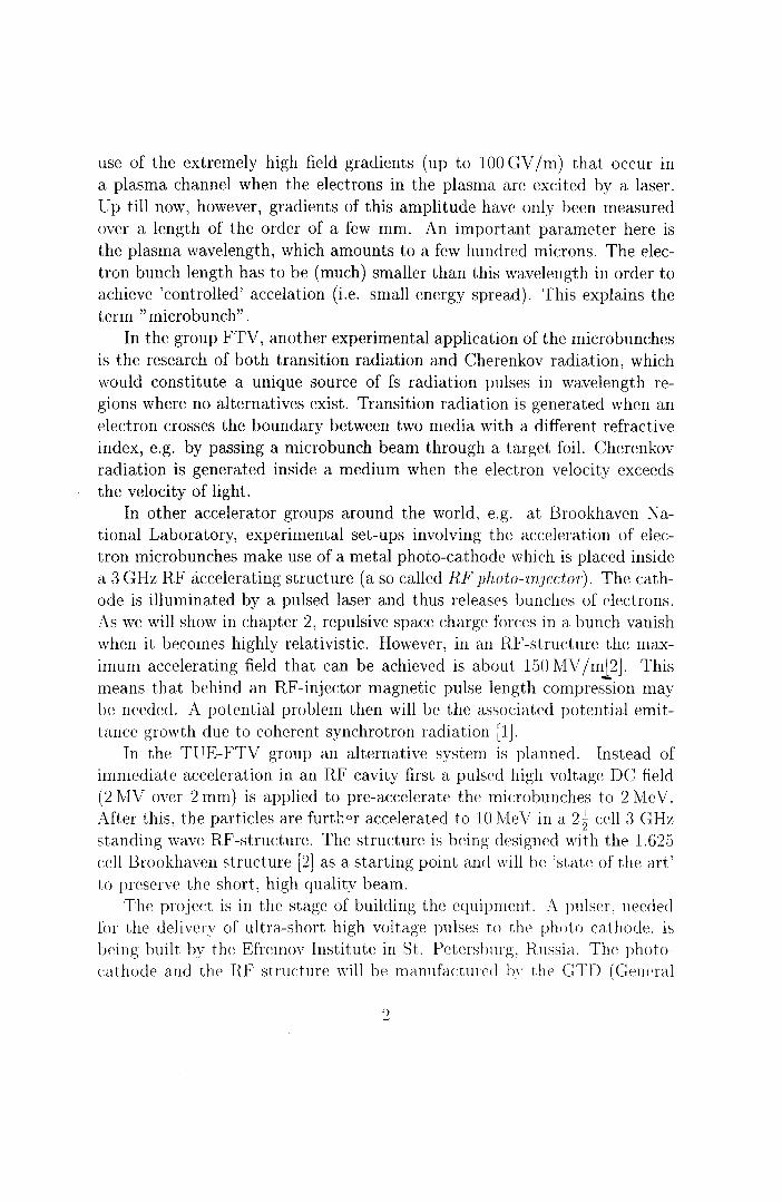
In figure 1.1 the experimental set-up that is being constructed is shown. Dimensions are not drawn to scale. The high voltage pulses are delivered by a laser triggered spark gap (LTS) which is conneeteel to a Tesla coil. The LTS acts like an uitrafast switch (connection time about Hl ns). The titanium sapphire laser is used both for illuminating the photo cathode and triggering the LTS.

The operating frequency will be 0.1 Hz. One c:yde c:an be described as follows. The master oscillator (MO) triggers the Ncl:YAG amplifier (NYA). The NYA takesabout 5 ps to operate. Aftera few JLS thc :..ro senels its signal to thc modulator of the klystron causing it to fill the caYity with standing waves ( filling time a few tts, 2ps assumed). After a delaY time D 1 the Tesla c:oil is triggered. It takes about 1 ps to reach its n>ltage after which it is

2 Pulsar Physics, Utrecht

3

'TJ (D ...........

~a;s ·:.:,..... ......

0 @ ...... f-'

** ~I

Tesla coil 2MV -7

~ciE"gcod

bucking coil

tJ,FY'Ab": ~J!lplitJ~~:

trigger1' signa! 0.1 Hz

master oscillator 3 GHz

klystron lOMW

RF cavity

• •• optica! • •switch

75 MHz -7

phase loek

I~

Ti:S oscillator

Ti:S amplifier

optica! switch

anode L_ laser beam I sen:,i,t,',~~;~parent

~ nu.--''"""----~"·"-~ n....__----~~---~-r- ---------=q-photo cathod

as er triggered I--sparkgap -7

I

1'1 C8JC8J I lllllTOI"~----------------------------------11

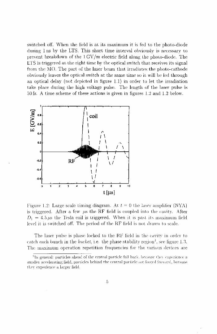
switched off. When the field is at its maximum it is fed to the photo-diode cluring 1 ns by the LTS. This short time interval obviously is necessary to prevent breakclown of the 1 GV /m electric field along the photo-diocle. The LTS is triggerecl at the right time by the optical switch that receives its signa! from the MO. The part of the laser beam that irradiates the photo-cathode obviously leaves the optica! switch at the same time so it will be led through an optica! clelay ( not depicted in figure 1.1) in order to let the irradiation take place during the high voltage pulse. The length of the laser pulse is 50 fs. A time scheme of these actions is given in figures 1.2 and 1.2 below.

8 ........ 0.8

>­Q, 0.

(.I.J 0.4

0.2

..().2

..().4

..().6

0 2 3 4

~ coil \

\

l I

5 6 7 8 9 10

t [~s]

Figure 1.2: Large scale timing diagram. At t = 0 the laser amplifier (NYA) is triggered. After a fcw JLS the RF field is coupl(~d iuto the cavity. After D 1 = 4.5ps the Tesla coil is triggered. When it is past its maximum field level it is switched of[ The period of the RF field is uot drawu to scalP.

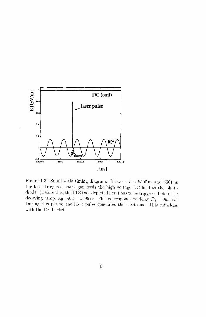
The laser pulse is phase lockeel to the RF field in the cavit\· iu order to catch each bunch in the bucket, i.e. the phase stability region 3

, see figure 1.3. The maximum operation repetition frequenties for t he \'arions deviccs a.re

3 In genera!: particles aheacl of the central partiele fall back. hecanse theY ('XJ.Wriencc a smaller accelerating field, particles behincl the central partiele are forced fon\·a.rd, bccause t heY (~xperiencc a largcr field.

~ 1~----------------------------~ ..§ DC (coil) > (!) 0.8

'--'

rJ.l _......laser pulse

0.6

0.4

0.2

t [ns]

Figure 1.3: Small scale timing diagram. Between t = 5500 ns and 5501 ns the laser triggered spark gap feeels the high voltage DC field to the photo diode. (Before this, the LTS (not depicted here) has to he triggered before the decaying ramp, e.g. at t = 5495 ns. This conespouds to delay D 2 = 995 ns.) During this period the laser pulse generates the electrons. This coincides with the R.F bucket.

6

respectively 100Hz for the klystron, 1 kHz for the LTS, 10Hz for the NYA and 0.1 Hz for the Tesla coil. The latter clearly forms the bottleneck.

In this thesis, as alternatives to the 2~ cell Brookhaven-type RF structure various travelling and standing wave structures, will be considered, see the next section. The Brookhaven-type structure is being investigated by Van der Geer and De Loos.

1.3 Contents of this report

The following two chapters contain theoretica! issues, such as RF-theory and beam characteristics. Chapter 4 starts with a short description of GPT and describes the simulated microbunch. Furthermore it contains results of sim­ulations in the Linac-10 and the RTME accelerating cavity, both for a single partiele and a whole bunch . These accelerating structures are described in chapter 2. Figures that will be shown are plots of the evoh1tion of the radial emittance and the bunch length insiele the accelerators. Other figures show the positon of the individual particles in e.g. the longitudinal phase space. Several results are compared to the case of zero space charge repulsion, to determine its impact on the beam parameters.

Chapter 5 starts with a description of the code Poisson/Superfish and describes results of simulations in q- and 2~-cell 'nose-cone' cell cavities. The structures are modeled with the Poisson/Superfish group of codes (see chapter 4.). Using these codes cavity parameters of interest are calculated and compared to the Brookhaven-type structure. Chapter 6 discusses the main results and the conclusions to be drawn.

7

Chapter 2

Radio Frequency Accelerating Structures

2.1 Standing Wave RF-structures

The standing wave structures investigated in this report are the accelerating cavity of the Racetrack Microtron Eindhoven (RTME, realized in 1996) and structures derived from it. A description of the RTME cavity will be given further on in this chapter. First several theoretica! issues will be cliscussed.

2.1.1 The Standing Wave Linac

A standing wave linac consists of an array of coupled cavity resonators, or briefiy, cavities. A cavity is made of a conducting materiaL The acceleration of particles is accomplished by using AC electromagnetic fields at high fre­quencies (100 MHz- 20GHz), which, because of historica! reasons, are called radio frequencies (RF fields). The power needeel to lmild up these fields can he delivered by a magnetron or a klystron. In a single cavit,· an infinite number of electromagnetic field r.-:.odes can exist that corresponcl to solu­tions of ?\Iaxwell's equations. These field modes are called rescmant modes. Tlw,· are the result of travelling waves that are refiected (iclcalh·) infinitdy 1nam· times at the bounclaries of the cavity. The lm\'<~st transverse magnetic: resonant mode that c:an r~xist in a cylindrical cavit,· is tlw so-('alled TJJ010

nwdr'. This mode is the one that has properties which makP it wrY snitahlr~ fm ac:c:elerating charged particles: the dectrornagrH'tif' field is rotationalh· snnf'tric. i t is indcp(~IHlf'nt of the ca,·i ty lcngth aud all cl<'ct ti(' field liues

8

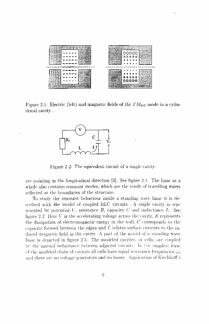
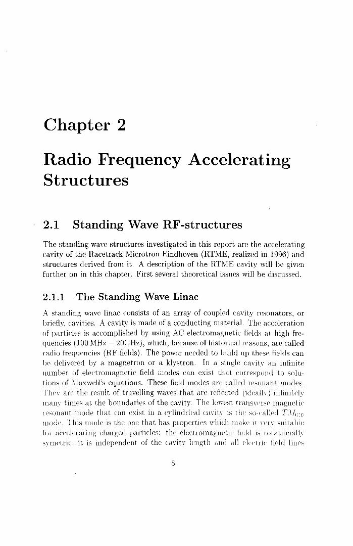
Figure 2.1: Electric (left) and magnetic fieldsoftheT M010 mode in a cylin­drical cavity.

Figure 2.2: The equivalent circuit of a single c:avity.

are pointing in the longituclinal elireetion [3]. See figure 2 .1. The linac as a whole also contains resonant modes, which are the result of travelling waves refiected at the bounclaries of the structure.

To study the resonant behaviour insiele a standing wave linac it is ele­scribed with the moelel of coupled RLC circuits. A single c:avity is rep­resenteel by potential V resistance R, capacity C awl induc:tance L. See figure 2.2. Here V is the accelerating voltage across tlw cavity, R represents the dissipation of elec:tromagnetic energy in the walL C corresponds to thc capacity formeel between the edges and L relates surface currcnts to the in­dnc:rd magnetic: field in the cavity. A part of tlw model of a standing vvave linac: is depic:ted in figure 2.3. The modeled cavities. m cells. arf' coupl(~d b,- t lw mut u al incluc:tancc between adjacent circuits. In t he simpll'st fonn of thc modeled c:hain of C<t\·ities all c:ells have equal U'SotJanu~ frcquencics ~0 awl therP are no nlltage generators and no losses. _-\pplicaticm of Kirchhoff's

9

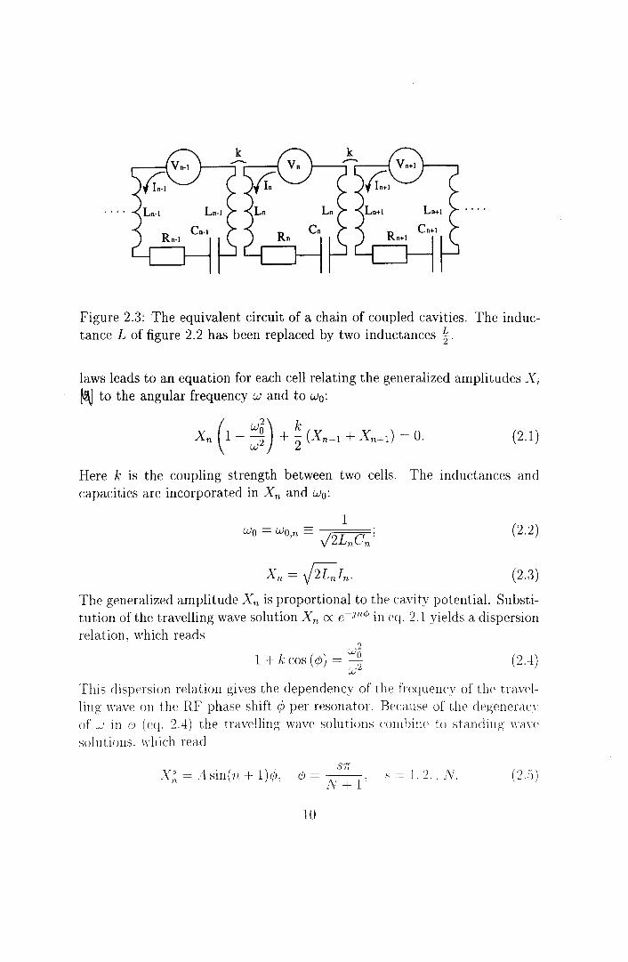
Figure 2.3: The equivalent circuit of a chain of coupled cavities. The induc­tance L of figure 2.2 has been replaced by two inductances ~.

laws leads to an equation for each cell relating the generalized amplitudes Xi ~ to the angular frequency w and to w0 :

(2.1)

Here k is the coupling strength between two cells. The inductances and capacities are incorporated in Xn and w0 :

1 w =w = · 0 O,n- J2LnCn'

(2.2)

(2.3)

The generalized amplitude Xn is proportional to the cavity potential. Substi­tution of the travelling wave solution Xn ex c-jn</J in eq. 2.1 yields a dispersion relation, which reads

2

k ( ' Wo 1 + cos C/)) = 2 w

(2.-±)

This dispersion relation gives the dependency of the frequency of the trawl­liug wave on the RF phase shift rjJ per resonator. Beumse of the degenen\CY of ~· in o ( eq. 2.4) the travelling wave sol u ti ons combine to standing \\(-\\\' solntions. \Yhich read

X;~ =A sin(n + 1)rjy, SJr

r/J= N+l'

10

_" = 1. 2 . .. N.

For a chain of N cells the number of resonant modes s is N . It can be shown that in the case of a non-ideal structure, where the resonant modes are shifted due to small frequency errors in the individual cavities, the optima! mode is the 1r /2 -mode. In the 7r /2 -mode only half of the cells contain energy. These cells we call accelerating cells, their empty neighbouring cells we call coupZing cells. Because the coupling cells contain no field their shape can be optimized to imprave the coupling between the accelerating cells [~l

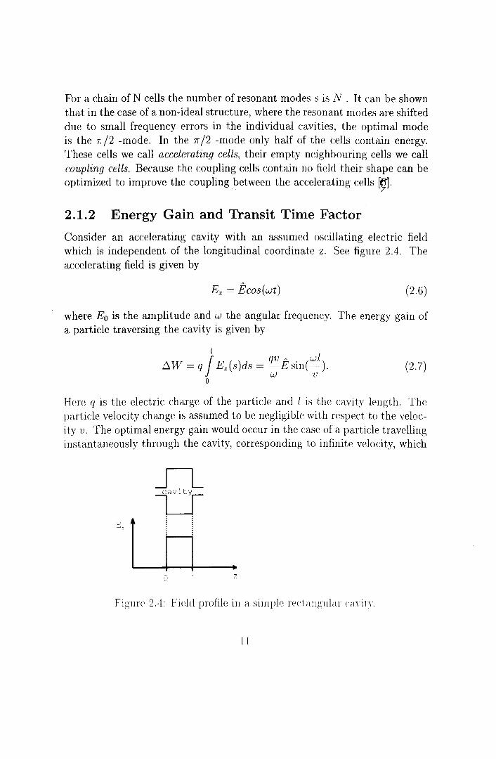
2 .1. 2 Energy Gain and Transit Time Factor

Consicier an accelerating cavity with an assumed oscillating electric field which is independent of the longitudinal coordinate z. See figure 2.4. The accelerating field is given by

Ez = Êcos(wt) (2.6)

where E0 is the amplitude and w the angular frequency. The energy gain of a partiele traversing the cavity is given by

l

I qv A wl ~W = q Ez(s)ds = -E sin(-).

W V (2.7)

0

Here q is the electric charge of the partiele and l is the cavity length. The partiele velocity change is assumed to be negligible with respect to the veloe­i ty v. The optima! energy gain woulel occur in the case of a partiele travelling instantaneously through the cavity, conesponding to infinite velocity, which

__fL_

L

t H D • () 1 z

Figure 2.4: Field profile in a sim ple rec:taugular <<lYi tT

11

is not a physical situation, so it is much easier to look at the case w = 0. Then the energy gainis given by

l

~Ww=O = q j Ez(s)ds = qÊl. 0

(2.8)

N ow, the transit time factor T is defined as the ratio of the energy gain and the optimal energy gain. So

~W V w[ T = ~W =-sin(-).

w=O wl V (2.9)

One notices that a shorter cavity length increases the transit time factor, but the limit here is break down of the electric field. In the more general case of a z-dependent field, the transit time factor is calculated as

l

I I Ezcos(wt)dzj T= ------------ (2.10)

Define V as V = I Ezdz, then the energy gain of the partiele is given by 0

~W = qVTcosrjy, (2.11)

where rjy is the RF phase when the partiele enters thc cavity [lq.

2.1.3 Shunt lmpedance·

The major part of the power that is injected into an RF structure is dissipated in the cavity walls. There are also power losses in thc transmission line between the klystron and the cavity as well as losses duc to rdiection at the RF input of the cavity. Here we only will consider thc losses at tlw cavity walls ( Pdiss). Pdiss aprwars to be proportional to the square of the energy gain ~ vF. The shunt imperianee Rs is defined by

' •2 p ---dzss - [J

l.s

12

(2.12)

and is a measure for the power required to achieve a certain energy gain. The higher the shunt impedance, the less power is needed. Another definition that is often used defines the shunt impedance per unit length r 8 by

dPdiss -E;(z) dz T 8

(2.13)

where dPdissl dz is the power dissipation per unit length and Ez is the electric field as seen by the particleij].

2.1.4 Quality Factor, Stored Energy and Filling Time

The unloaded quality factor Q of a cavity is defined as

u Q = w-, (2.14)

Pdiss which is the same as 21r times the stored energy U divided by the energy dissipated in a single RF period. 'Unloaded' means that energy flowing out of the cavity back to the klystron or to the electron beam is not taken into account.

The quality factor determines the time that is needed to build up the fields in a cavity or to let the fields decay. This can be seen by writing eq. 2.14 a little different:

dU U -=-w-dt Q'

(2.15)

because the power dissipated in the walls equals the rate at which the stored energy decreases:

Integration of eq. 2.15 yields

U ex e-wt/Q.

Si nee U ex E 2 ( E represents electric field) we have

E ex e-t/Tr '

where

is t lw .fi:lling tune of the <:clYi ty.

2Q TJ =:­

w

(2.16)

(2.17)

(2.18)

(:2.19)

So a c:avitv with a higher Q requires less power but takes more time to lmild up elc~ctrornagnetic: fields QJ.

13

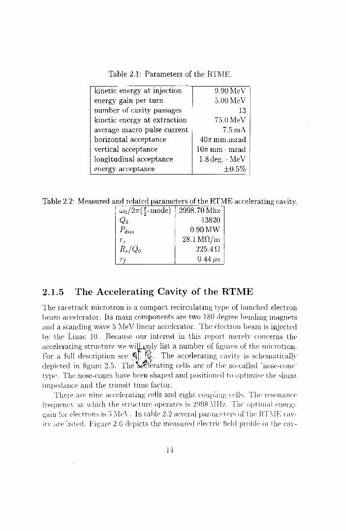
Table 2.1: Parameters of the RTME.

kinetic energy at injection energy gain per turn number of cavity passages kinetic energy at extraction average macro pulse current horizontal acceptance vertical acceptance longitudinal acceptance energy acceptance

9.90MeV 5.00 Me V

13 75.0MeV

7.5mA 407r mm.mrad

l07r mm · mrad 1.8deg. · MeV

±0.5%

Table 2.2: Measured and related parameters of the RTME accelerating cavity. w0 /27r(~-mode) 2998.70 Mhz Qo 13820 Pdiss 0.90 MW

28.1 Mf2/m 225.4 n 0.44/LS

2.1.5 The Accelerating Cavity of the RTME

The racetrack mierotrou is a compact recirculating type of bunched electron beam accelerator. lts main components are two 180 degree hending magnets and a standing wave 5 fi;Ie V linear accelerator. The electron beam is injected by the Linac 10. Because our interest in this report merelv concerns the accelerating structure we wi~nly list a number of figmes of the rnicrotron. For. a ful~ cie.scription see [~], . ] . ~he acceleratii~g cavity is sd~ernaticall~~ dep1cted m figure 2.5. The leratmg celb are of tlw so-called nose-cone type. The nose-cones have heen shaped and positionl'd to optimise the shunt impedance and the transit time factor.

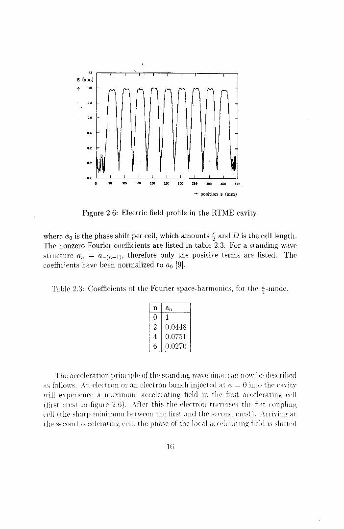
There are nine accelerating cells and eight c:oupling u'lls. The resonancf' frecp!cnc,· at which the structure operates is 2998 .\I Hz. Thf' optima! C'ltergy gain for electronsis 3 .\Ie\·. In table 2.2 several par<nneters of tlw RT\IE cm·­i t,· are list ecl. Figure 2. 6 depiets the measurcd elect ric field profile i u t he Gl\"-

cru:;;:;t-l'liou AA

1------------ 4G t'ln ----------------J

Figme 2.5: Schematic layout of the RTME cavity.

ity ~· It shows the absolute values of the amplitude E 2 , a plot of the actual amplitude at a fixecl time woulel show alternating maxima and minima. The electric field profile has been calculated with the Poisson/Snperfish code (see chapter 5) by De Leeuw ancl the longitudinal electric field Ez can be written as a Fomier series expansion in longituclinal spac:e harmonies:

+oo

E ( . t) - """' a E I ( '· r·)('.J(w·t.-A:" c I z z, r' . - L n Oz 0 (,,n . . (2.20) n=-oo

where a11

are the Fomier coefficients, Eaz is the amplitude. 10 is thc ~ero-th order moclified Bessel function: àn is defined by

(2.21)

Here k = :;:: is the total \\';wenumber and k11 is the longitndiwd ml\'f'llllmhr'r: I

c/Yo + 2'7f71 k ----­"- D

Lï

(2.22)

1.% I I -1

E (a.u.)

t 1.CI r-M M M M ,_" M r"'' M 11

0.~

o.e

OA

0.2 r

M ~ ~ ~:<

I I I I I I

0 5(] 100 ~ 2CQ :z.so 300 3!50 -100 ~ soo

4 poiJition 3 (mm)

Figure 2.6: Electric field profile in the RTME cavity.

where <Po is the phase shift per cell, which amounts i and D is the celllength. The nonzero Fourier coefficients are listed in table 2.3. For a standing wave structure an = a-(n+l), therefore only the positive terms are listeeL The coefficients have been normalized to a0 [9].

Table 2.3: Coefficients of the Fourier space-hannonics, for the ~-mode.

n an 0 1 2 0.0448 4 0.0751 6 0.0270

Thc ac:celeration principle of the standing wavP liuac: eau now lw clesnibed as follows . .-\n electron or an electron bunch injected at q; = 0 into the (<-n·it~' \\·ill experienc:e a maximum ac:celerating field in the first ;-H·cderating cdl ( first crest in tigure 2. 6). Aft. er this the electron tniY<'rses the ti at con pling ce ll ( t he sharp minimum bdween the first and the secoud crest). Ani ,-ing a 1

t he second accclerating cc!L the phase of the loe-t! <-HT<'lerating fi<'ld is shiftr~d

16

by 1r and the particle(s) again will feel maximum acceleration, and so on. The coefficients in table 2.3 are incorporated in the modeled cavity used

in the simulations in chapter 4.

2.2 The TUE Traveling Wave Linac 10

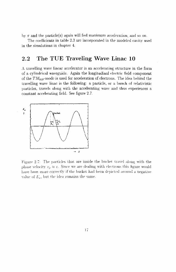
A travelling wave linear accelerator is an accelerating structure in the form of a cylindrical waveguide. Again the longitudinal electric field component of the T M010-mode is used for acceleration of electrons. The idea behind the travelling wave linac is the following: a particle, or a bunch of relativist.ic particles, travels along with the accelerating wave and thus experiences a constant accelerating field. See figure 2. 7.

t

~ ".i

..... z

Figure 2. 7: The particles that are inside the bucket travel along with the pltase velocity t'p ;::::: c. Since we are dealing with dectrons this tigure would have been more correc:th· if t.he bucket had been depicted anmnd a negative \<due of Ez, but the idea remains the same.

17

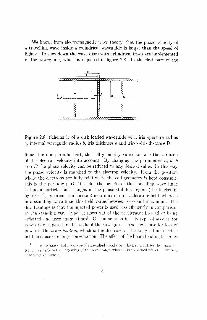
We know, from electromagnetic wave theory, that the phase velocity of a travelling wave inside a cylindrical waveguide is larger than the speed of light c. To slow down the wave discs with cylindrical irises are implemented m the waveguide, which is depicted in figure 2.8. In the first part of the

D

r d

L· ~------------ - ~ - ~---+'=------

Figure 2.8: Schematic of a disk loaded waveguide with iris aperture radius a, internal waveguide radius b, iris thickness b and iris-to-iris elistance D.

linac, the non-periadie part, the cell geometry varies to take the varation of the electron velocity into account. By changing the parameters a, d, b and D the phase velocity can be reduced to any desired value. In this way the phase velocity is matched to the electron velocity. From the position where the electrous are fully relativistic the cell geometry is kept constant, this is the periadie part [10]. So, the benefit of the travelling wave linac is that a particle, once caught in the phase stability region ( the bucket in figme 2. 7), experiences a constant near maximum ac:c:elerating field, whereas in a standing wave linac this field varies between zero and maximum. The disadvantage is that the injected power is used less efficiPntly in c:omparison to the standing wave type: it ftows out of the accelerator instead of bcing rPftected and used many times1

. Of course, ab:1 in this t\'IW of accelerator po\\'er is dissipated in the walls of the waveguiclc. Another c:ause for loss of po\\'er is the beam loading, which is the decreasc of th<' longitudinal dectric tie lel. hecause of energv conservation. The effect of the h(~am lo<Hling heemnes

1 Tlwrl' <HP linacs that makt• nse of aso-called circulator. \\·hich n·l·ircnlatl's tlw .. lllll!Sl'd ..

HF jlO\\Tr back to the heginning of the accelerator, wlwre it is cmt!lJinl'd \Yith tlw kh·stmn

of ttt<lgttctrmt pmYer.

18

! 4

I I I I

I : : I I

12 13

Figure 2.9: The Linac 10: 1 )trigger pulse generator, 2)pulse forming network, 3)magnetron, 4)RF window, 5)isolator, 6)group of focusing coils, 7)steering coils, 8)electron gun, 9)focusing coil, 10)group of focusing coils, ll)RF load, 12)insulating disk, 13)Faraday cup

noticable in the case of acceleration of many micropulses (bunches) within one macropulse (period during which a linac is filled with RF fields).

The TUE Linac 10 is clepicted in figure 2.9. Some parameters are listeel in table 2.4. It is used to inject electron bunches into the RTME. Electron bunches are released from the catbode by thermal emission instead of photo emission ( the catbode has the form of a me tal wire instead of a surface). In the simulations performeel in chapter 4, the linac is modeled as if it were fully periodic, and we will see that the accelerating field in the first part of the linac does not match the electron velocity for relatively slow electrons. Of the parts depicted in figure 2.2, only the focusing coils armmei the periodic: part are used in the model. The longitudinal electric field E 2 (,c:, r. t) in the periodic part can again be written as a series expansion in longitudinal spac<~ harmonies (eq. 2.20). For the Lina.c:-10, c/Jo = ~; [10]. Tlwse Fomierc:oetfic:imts also have been calculatcd with Poisson/Superfish ancl are listcel in tablc 2 .. J.

The dectric field amplitude Eaz in eq. 2.20 is ouh· c:oustant in the ideal case of an infinite qualitY factor and zero beam ClllT('ll1. Iu practice. t he power of t he waw deca,·s a long the linac. clue to bot h di ss i pation aud hcam loading. Tlw amplitude E20 (z) of the longitudinal <'lectric field has lw<'n computecl for \<Uious (final) bcam currents [Hl]. se<' figme 2.10.

19

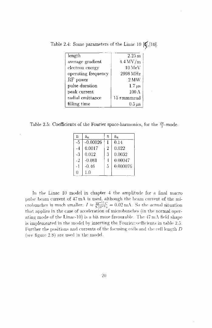
Table 2.4: Some parameters of the Linac 10 [~,[10].

length average gradient electron energy operating frequency RF power pulse duration peak current radial emittance filling time

2.25m 4.4MV/m

10MeV 2998 MHz

2MW 1. 7 fLS

100A 157rmmmrad

0.5 JLS

Table 2.5: Coefficients of the Fourier space-harmonics, for the 217r -mode.

n an n an -5 -0.00026 1 0.14 -4 0.0017 2 0.022 -3 0.012 3 0.0032 -2 -0.081 4 0.00047 -1 -0.46 0 0.000076 0 1.0

In the Linac 10 model in chapter 4 the amplitude for a final macro pulse beam cttrrent of 47 mA is used, although the bcam c:urrent of the mi­crobunches is muc:h smaller: I ~ ;01~~

0

/~ = 0.02 mA. So thc actual situation that applies in the case of acceleration of microbuudws (in the normal oper­atinp; mode of the Linac-10) is a bit more favourahle. The 47mA field shape is implementeel in the model by inserting the Fouriei·:·rwffic:ients in Ltbl(~ 2.5. Further the positions and currents of the focusing coils ancl tlw celllcngth D (see figure 2.8) are used in the model.

20

8 ~~~~~~~~~~~~~ E, (MV/m)

t 6

4

2

50 100 150 200 250 ~ z (cm)

Figure 2.10: The amplitude of the axiallongitudinal component of the elec:tric: field as a func:tion of the longitudinal c:o-ordinate. Here Ezo is noted as Ez.

21

Chapter 3

Emittance and Space Charge Farces

In this chapter one of the most important parameters of electron bunches is discussed: the emittance. First the concept is explained, after which several de.finitions are given. Finally a simple model for the space charge farces inside a relativistic bunch is diswssed.

3.1 Phase Space and Emittance

Every single partiele can be represented by a point in the six-dimensional phase space. There are three dimensions for both the position of the partiele

(:1:, y, z) and its velocitv, or, more correctly, its momenturn (PnPy,Pz)· We can divide this hyperspace in three two-dimensional phase spaces, namely the transversal ((:z:,px) and (y,py)) and longitudinal ((:::,pz) phase spaces. A lmnch of electrous can thus be represented by a nuHlher of points in phase space. :'\ ow, Liov.ville 's theorem, valiel for Harnil tonian svstems (i.e. space charge forces are not included), states that the hypen·olume occupied bY a lmnch of particles. the cmittance, has a constant value. Tllt t:wo-dimensional projc~ction of the ernittance on either onc of thc transversal phase spa('(-'S or one the longi tudinal ph a se space is ca.lled thc horizont<ll ( vert i caL radial) emi t t a nee a nel t he longi t udinal erni ttance respect i w h·.

In practice. enlittance is definecl in termsof di,·cTgi'lW<' (tr<lllswrsal) m <'lHTg\· (longitudinal) rather than moHwntum. In figm<' :u til<' !!lotion of <1

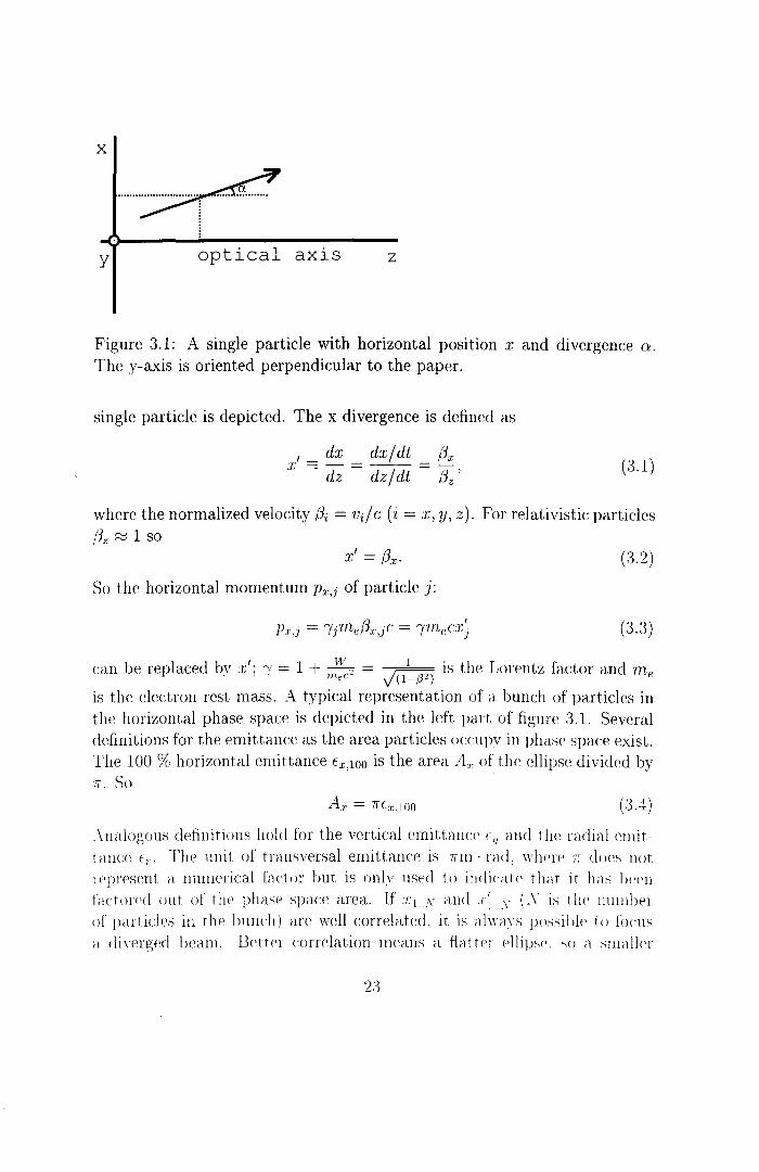
x

·····~ y optical axis z

Figure 3.1: A single partiele with horizontal position .T and divergence o:. The y-axis is oriented perpendicular to the paper.

single partiele is depicted. The x divergence is defined as

1 _ dx dxjdt f3x x--=--=-

- dz dz/dt f3z' (3.1)

where the normalized velocity f3i = vdc (i= x, y, z). For relativistic particles {Jz ~ 1 SO

x' = f3x· (3.2)

So the horizontal momenturn Px,j of partiele j:

(3.3)

can be replaced bv :r'; r = 1 + w 2 = p is the Lorentz factor and me · me c ( 1-{J2) ~

is tlw electron rest mass. A typical representation of a bunch of particles in the horizontal phase space is depicted in the left part of figure 3.1. Several definitions for the emittance as the area particles occupv in phase space exist. The 100 % horizontal emittance Ex,loo is the area A, of the ellipse divided by 11. So

Ax = 7rE.7:,100 (3.4)

Analogous clefinitions hold for the vertical emittauc<' f,1 and t he radial c~mit­tancc f 1.. The unit of trausversal ernittance is 7flll ·rad, wher<' 11 does uot !'('present a numerical factor but is onlv used to iudicat<' that it has lH'eu fa ct orcd out of t h<' ph a se space area. If :r: t. 1\' aud .1

11 . :\ CY is t lw lllllnber

of particles i u t Iw bunch) are well correlatccL i t is ;tl wcn·s possi hl<' to focus " din~rgcd beam. Bette'!' correlation means a fiat t<'l <'liips<'. so ;) suutll<'r

23

x' x'

x

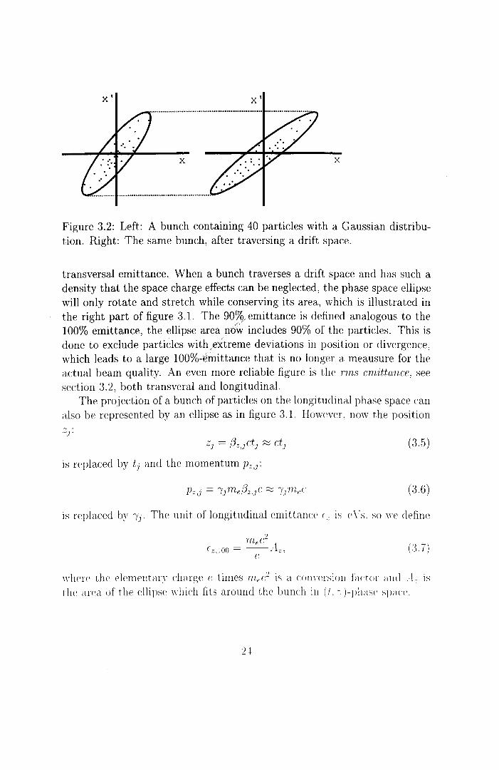
Figure 3.2: Left: A bunch containing 40 particles with a Gaussian distribu­tion. Right: The same bunch, after traversing a drift space.

transversal emittance. When a bunch traverses a drift space and has such a density that the space charge effectscan be neglected, the phase space ellipse will only rotate and stretch while conserving its area, which is illustrated in the right part of figure 3.1. The 90% emi ttance is defined analogous to the 100% emittance, the ellipse area no~ includes 90% of the particles. This is done to exclude partiCles with .extreme deviations in position or divergence, which leads to a large 100%-èmittance that is no longer a meausure for the actual beam quality. An even more reliable figure is the rm.s erndtance, see section 3.2, both transveral and longitudinal.

The projection of a bunch of particles on the longitudinal phase space can also be represented by an ellipse as in figure 3.1. However, now the position

Zj = fJz,jCtj ;:::::: ctj

is replaced by tj and the momenturn Pz,{

(3.5)

(3.6)

is replaced by rj· The unit of longitudinal emittance f: 1s e\'s. so wedefine

(3.7)

wher<' the dementan· charge e times mcr:2 is a conwrsiou factor awl _c\. 1s the ;m~a of the ellipse "·hich fits around the lmnch iu (t. ~. )-phas<' span'.

3.1.1 Normalizing the Emittance

From eq. 3.3 we see that the radial emittance scales with the area in (:r, Px)­space as ~- 1 . So, just by accelerating a bunch, the emittance decreases because of relativity. This effect is called adiabatic shrinkage. If we want to know how the horizontal emittance is developing during acceleration, re­gardless of relativic effects, we use the normalized emittance, which is defined

as -1

Ex,n =I Ex.

Analogous definitons apply for Ey,n and Er,n·

3.2 Definitions used in this report.

(3.8)

The emittance values used in the results in chapters 3 and 4 are all normalizeel rms values.

When spoken of horizontal emittance Ex the following clefinition is referrecl

to1:

with

f,. = 4rvVx 2 · x' 2 - x x'c2

L I c c C

{

Xe= .T- X,

Yc = Y- fl,

.T~ = I (f-Jx - f3.r) :u:: = I (!3v - f3,;)

The bars clenote values averagecl over the inclividual particles.

(3.9)

(3.10)

vVhen a cylindrical symmetrie beam rotates around the ;;-axis (e.g. when inHm~nced by an external solenoicl field, as is the case with the Linac 10), then' is astrong correlation between both :r, y' and T', :IJ rather than bet\veen hoth :r, :r' and y, y'. This leads to large values of f1 <Uld f.,1 . To compensate for this effect, the radial emittance Er is calculated in the fom-dimensional (:r, :1:', y, y')-phase space a.s2

fr,rr11s = f:r,rrns · fy,rm.s- 1.1:,.:1/c · T~.y;.- Tr,lj; · ./:;.:IJ,I. c~.n)

It should he noted that the definitions for f 1 and f,1 usl'd in cq. >U1 differ from the one in eq. 3.9:

1 In G PT. t his is t Iw pro~ram ncmi:J:. 2 In GPT. this t.he program nemirrms.

and

with

fx,rms =/x~· X~2 - XcX~2

-/2 12 --,2 fy,rms - Yc · Yc - YcYc '

{

x -x- x c- '

Yc = Y- y, < = "( (f3x - fJJ:) y~ = "( (f3y - /3y)

(3.12)

(3.13)

(3.14)

The differences between eqs. 3.9 and 3.12 are the factor 4 and the aver­aging of the Lorentz factor.

Note: by convention, the unit of the transversal rms emittances mentioneet so far also is 1r mm.mrad, despite the fact that no ellipse is invalveel in the calculation.

The normalizeel longitudinal rms emittance is defined by:l

with

2 mee;-- -2 tz,rms = -- t~ · "(~ - lc"fc ,

e

te= t-I, "te = "(- "(.

(3.15)

(3.16)

The factor in front of the square root sign is used to corm~rt the units from [J · s] to [eV · s].

3.3 Space Charge Forces-A Simple Model

In thc following, the electrit and the magnetic fon·rs that act upon a single electron, as a result of its interaction with thc space charge surrouncling the electron, will he investigatecl. The space charge is fomH:~d b~r a.ll the other elr~ctrons in the bunch. Here, the bunch is modeled as a cYlinder containing a homegeneons charge, sec figure 3.3. There are two fon·es actin12; on each single partic:le: a radial dectrostatic repulsivc force. awl a radia~],· actrac:tin• force that arises frorn the Lorentz force resulting flom thf' tnagnf'tic held neated ]l\· the co- travelling charged partic:les [11]:

F(r) = q(E,.- ,)cBo). (:3.1 ï)

\\"r• um applY Gauss' Law to an axial cin:ular disc \\"Îth t<Hlius R awl iu-

:1 I u G PT. this t lw progr;ml nemizrrns. 7

2G

2R

--- ----- - -- - _.-~~----/ 4 ~.~~ r..~ ~. I ~ ~~ ~

L

I~ \

~ \ ~ ~

--- ~

Figure 3.3: Homogeneously charged cylindrical model of an electron bunch.

finitesimal height h:

Integrating eq.3.18 yields

Hence

/ j Ê · ndA = Q I Eo

E Rh_ ph1rR2

R'27f ---­Eo

ER= LR. 2E0

Ncxt Ampere's Law is applied to the flat cylinder:

Intcgration yields

l Bds = JLo //.!:dJ. R

(J . Bo = -:JzR·

2EoC

Combining <'qs. :3.Hl. :3.:21 and 3.17 leads to

'2ï

(3.18)

(3.19)

(3.20)

(:3.21)

(:' ')')) ). __

()If the charge density depends on r, the expression looks somewhat different, but the factor ,-2 remains in the formula.

I t should be noted that the previous is only valid in the case L > > R, because otherwise the deviating electromagnetic fields near the edges have to be considered.

So in the ideal case of a homogeneously charged bunch of infinite length the Coulomb repulsion by the space charge is cancelled by its magnetic at­traction if the bunch is highly relativistic. The practical impheation of this is obvious: to minimize (normalized) emittance of an electron bunch it is nec­essary to accelerate it to highly relativistic energies right after its generation.

In the case of microbunches the situation is much more complicated. Now L < < R, so the effect of the longitudinal electric field is no longer negligible near the edges. Another difference in comparison to the simple model is that the attractive magnetic force depends on the longitudinal position inside the bunch.

28

Chapter 4

Microbunch Dynamics in the Linac 10 and the RTME Cavity

In this chapter the acceleration of a pre-accelerated 2 Me V microbunch in the TUE Linac 10 and the RTME cavity wilt be investigated. We are interested in the electric field gradients that are required for the preservation of the bunch, especialty the radial emittance and the bunch length. The chapter starts with a description of the computer code that has been used for the beam dynamics simulations in this report, tagether with a description of the 8imulated microbunch. Foltowing this, rewlts of simulations in the Linac 10 and the RTME cavity wilt be presented.

4.1 The General Partiele Tracer Code

The General Partiele Tracer (GPT) code [12] is a completely three-dimensional simulation code for the study of charged partiele dynamics in electromag­netic fields. Electromagnetic fields are calculated from elements that the user specifies, and which can be combinc~d to a beam line. These beamline dements are represented by their indiviclual elec:tromagnctic fielcls. The to­tal electrornagnetic: field at each temporal and spatial positiou is found lw superposition of the tielels of the elements and is iuserted in a .h:eld me.sh. which is a discretized representation of the loc:al ficlds. In case of a bunch of c:harged particles, it is possible to bring space dwn;e interaction into ac­count. The particles <HP representecl by homogeneouslv charged spheres, t he nw.cmparticles. Each macropartiele represents a large rmmlwr of indi,·id-

29

ual particles. In the case of electrans a macropartiele has elec:tric charge -ne and mass nme, where n is the number of electrans incorporated in the macroparticle. For each macropartiele an equation of motion containing the total electromagnetic field at the nearest mesh point has to be solved. This field is a superposition of the 'beamline field' and the Coulomb interaction of a macropartiele with its neighbours (which form the space charge). GPT uses a fifth order Runge-Kutta integrator to solve the relativistic equations of motion for the macroparticles in the time domain. The equations of motion do not contain the vector potential. This can lead to too large valnes of the calculated emittance inside beam line elements [13].

4.2 Description of the Simulated Microbunch

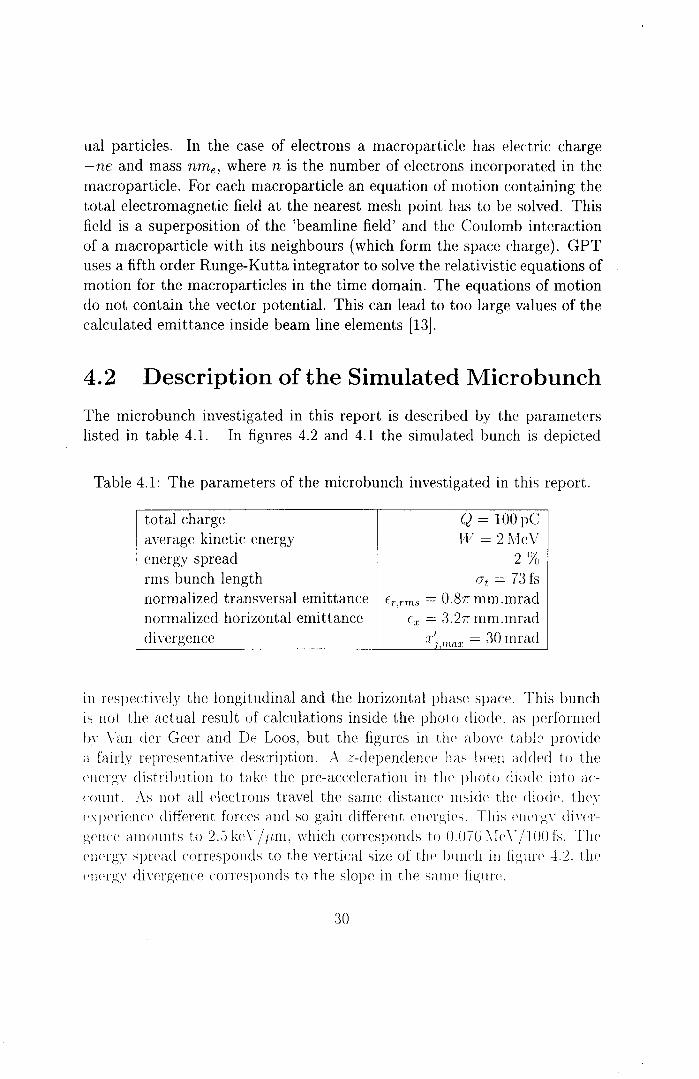
The microbunch investigated in this report is described by the parameters listed in table 4.1. In figures 4. 2 and 4.1 the simuiateel bunch is depicted

Table 4.1: The parameters of the microbunch investigated in this report.

total charge average kinetic energy energy spread rms bunch length normalizeel transversal emittance normalizeel horizontal emittance divergence

Q = 100pC T1V = 2 rvieV

2% CJt = 73 fs

Er,rms = 0.87r mm.mrad Ex = 3.27r mm.mrad

:r'7 "w:~· = 30 mrad

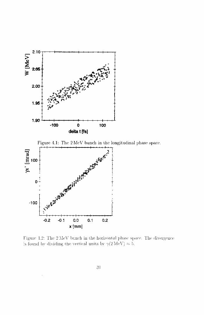
in respectin~ly the longitudinal and the horizontal phase space. This bunch is not the actual result of calculations insiele the photo diode, as performeel hv Van der Geer and De Loos, but tht: figures in the a bove ta bl:• provide ;1 faidy representative description. A z-clqwndenn' has 1H~<~Il ;Hld<~d to the <'ll<'l/2,V distri 1 m ti on to ta kc thc pre-acc:eleration in t Iw photo diode into ac­count. As not all electrous travel the sarnc distauc<' iusidc the diode. thcv <'xperience different forces aud so gain different Cll<'l/2;ies. This <'lH'lg\· diwr­g<'ncc ëUllOllltts to 2.5kc\);un, which corrcsponds to ll.07G\IeY/100fs. The <'Il<'l/.',Y spread c:orresponds to the vertical si ze of tlw 1 mnch i u hg m<' 1.:2. t.he <'ungv diwrgence <·.orrcsponcls to the slopc in the s;uw' hgme.

30

......., "0 E

2.10 ,..----+----+----+---4-+--+---r

2.00

1.95

1.90~~-+---------+-+-+-+-+-+-'+-~

-100 0 delta t [fs]

tOO

Figure 4.1: The 2 Me V bunch in the longitudinal phase spaee .

a 1oo

i

0 ' t

I -100

I ...

-0.2 -o. 1 0.0 0.1 0.2 x {mm]

F igme 4. 2: The 2 .\Ie V 1 mncb in the horizontal phas(' spe~c('. Thc di wrgcnce is fouud lw dividing tlw n'rtical units by 1(2 .\JrN) ~ :).

31

If the bunch could be rotateel in the longitudinal phase space (by using an compact optica! sytem of bending magnets, see chapter 3) to minimize the bunch length an estimated 100 fs would be attainable. \Vith an analogous system the opposite can be also be accomplished: a minimum energy spread of 2%.

It is also possible to perform a controlled rotation in the horizontal phase space (with the use of an optica! system consisting of quadrupole lenses). ('Controlled' means contrary to rotation caused by drifting.) The minimum attainable spot size amounts to about 40 J.Lm, the minimum attainable eliver­genee amounts to 5 mrad.

4.3 Simulations in the Linac-10

4.3.1 Single Partiele Simulations

The investigation of the behaviour of the electron bunch in the modeled trav­elling wave linac (cf. section 2.2) starts with calculations of the acceleration of a single electron at different values of the injection phase angle cf>. For simplicity the electron starts on the optica! axis, with zero divergence, so it is injected at t = 0, z = 0. The linac is positioned between z = 0 and z = 200cm. Since the axial E 2 -field bas a cos(wt- r/J) dependenee (real part of eq. 2.20), we expect the optimum phase angle to lw rp = 0, providecl that the partiele is highly relativistic. In that case the partiele experiences a field amplitude, decaying accorcling to tigure 2.10.

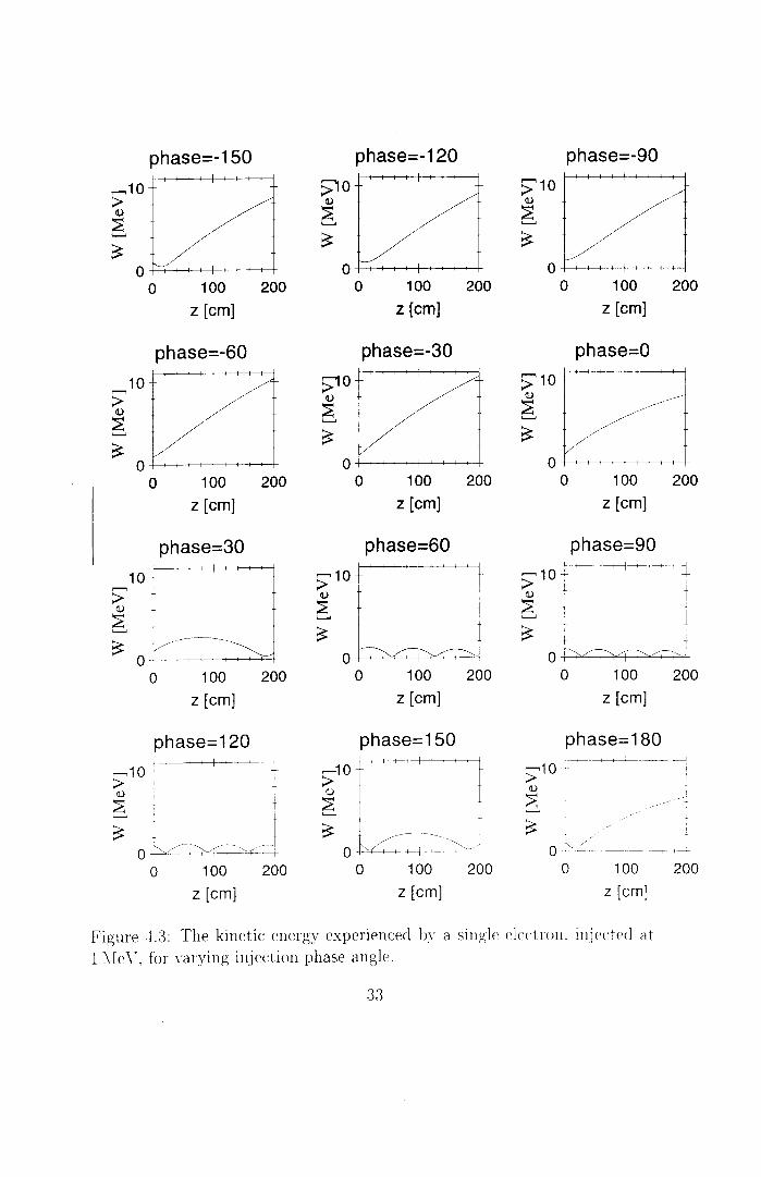
First, take a look at an electron with an in i ti al kinetic: ew~rgy of Hl = 1 Me V. Figure 4.3 shows that the optimum injection phase is not zero. but rather be­tween -60° ancl -30°. To explain the deviation of the optimum phase angle w.r.t. cf> = 0, we take a closer look at the accelerating field E2 • as seen by the P!ectron (figure 4.4). In fact, this curve is a simplification of the actual field, which is illustrated in appendix A. For the case c/J = 0 the field gradient is IEzl(200cm):::::::: 2 .\IV jm. so the electron experiences the field decaving more strong[~r than it does according to tigure 2.10, wlwre IE:I:::::::: :3./.\IV/m. The reason is that the electrou cannot keep up with tlw an:derating waw. which tn1wls at speed c. For (;J = -30° the electron trawls in <l held which n~maius alnlost constant. This occms hecause thc electron st;lrts ilhead of t h<' <T<'st of t he \\·aw. hut a long t he \\'aY the wan' catch<'S n p \Yi t h t Iw dectron. The resul t of hot h effects is t ha t the most effect i ve a< -cd<'tiltion t ak<'s plac<' fm

32

,........, 10 >

11)

~ .........,

~

phase=-150

100 200

z [cm]

phase=-60

100 200

z [cm]

phase=30

100 200

z [cm]

phase=120 : ----+-+--t-~--+-+--+------1

,........,1Q~ r > ' ~

11) I

; I 0 ~~- ~:_:::;:::::_-~;::;_

0 100 200

z [cm]

phase=-120

100 200

z [cm]

phase=-30

100 200

z [cm]

phase=60

0 -1-----+-~'---+-~+----+-~ 0 100 200

z [cm]

phase=150 ,........,1 0

1---+-+---+-+--+-----~-

~ t ~ .

~ l ~--~- : 0 ~ j------~cd

0 100 200

z [cm]

phase=-90

100 200

z [cm]

phase=O

100 200

z [cm]

phase=90 ,........, 1 o r+---+----o--+--1

~ r t ........., t l ~ I

0~04-~----,___j 0 100 200

z [cm]

phase=180 i -~1----+---+-~' ---~-+-

,........,10 ' >

11)

6 ~

0 '--0

-----r--~--~ -------r-- t-~

100 200

z [cm]

Figme 4.3: The kinet,ic cnergy experienced 1)\· a single electron. injected at

l \Ie\·, for \ëtrying injec:tion phase angle.

33

phase=-150 ,---, 1 0 8 ...._ > ~ 0 ..._.

~N

-1 0 -t----+--+-+--+-t--+-+--+---+----t-

0 100

z [cm]

200

phase=-60 ,---,1 0 8 ...._ > ~0 ..._.

ui' ~~-------r

-1 0 -t---+--+---+---+---t--+--+-+--+---+

0 100 200

z [cm)

phase=30 1 0 -+--+--+--+---+---t--+--+-+--+---+

'E ; 0 ///\1

-1 0 +-.---+--+---+-+----r-+---~-t-0 100 200

z [cm]

phase=120 ,---, 1 0 l-+-"-+-+-t--~ ~ E " I > V': /\) ~ 0 1' i. :

~ 1 I "T

LL.l i : ' --10 -'-~---~----+---------·~ 0 100 200

z [cm]

phase=-120 ,---, 1 0 _§ > ~ 0 ~ ~ f~...__-~-

-1 0 -r-+--+-+-+---t-+---+-+-+----t-

0 100

z [cm]

phase=-30 ,---, 1 0 8 > ~ 0 ..._.

200

N

LL.l L.__-~----

-1 0 -t---+--+-+--+-t-+--+-+---+---+

0 100

z [cm)

phase=60

200

1 0 -t---+--+-+----+---t---+-+-+---+---+

'E ...._

~ 0 ..._. N

~

-1 0 i-+-+-+-+-t-+-+

0 100

z [cm]

phase=150

200

E 10 r---+---+-t---+~+1

~ oj~///\j ~ 1 + -1 0 -t +- +--~t --r

0 100 200

z [cm]

phase=-90 ,---,10 8 ...._ > ~ 0 f\ ~ f"--~-----T

-1 0 -t-+--+-+--+-t--+---+--+---+----t-

0 100 200 I

z [cm]

phase=O ,---, 1 0 -r-+--+-+--+-t-+-+-+-+-t

8 ...._ > ~ 0 ..._.

N

~

-10

10 ,---,

E ...._

~ 0 ..._.

0 100

z [cm]

100

z [cm]

phase=180

u .. r j \._

-10 I - -----

200

200

0 100 200

z [cm]

Figme Lel: The accclerilting field Ez c:xperienced hY" singl<' electmu. iujected <ll 1 \kV.

3-1

this phase angle (<P = -30°). Figure 4.3 shows that between <P = 60° and <P = 90° the partiele is alternately accelerated and decelerated. In the corre­sponding plots in figure 4.4 it is shown that this is due to an alternating Ez­The partiele does experience acceleration, but its velocity stays too low to 'hang on' to the wave, thereupon the negative crest of the wave decelerates the electron again; this effect repeats itself.

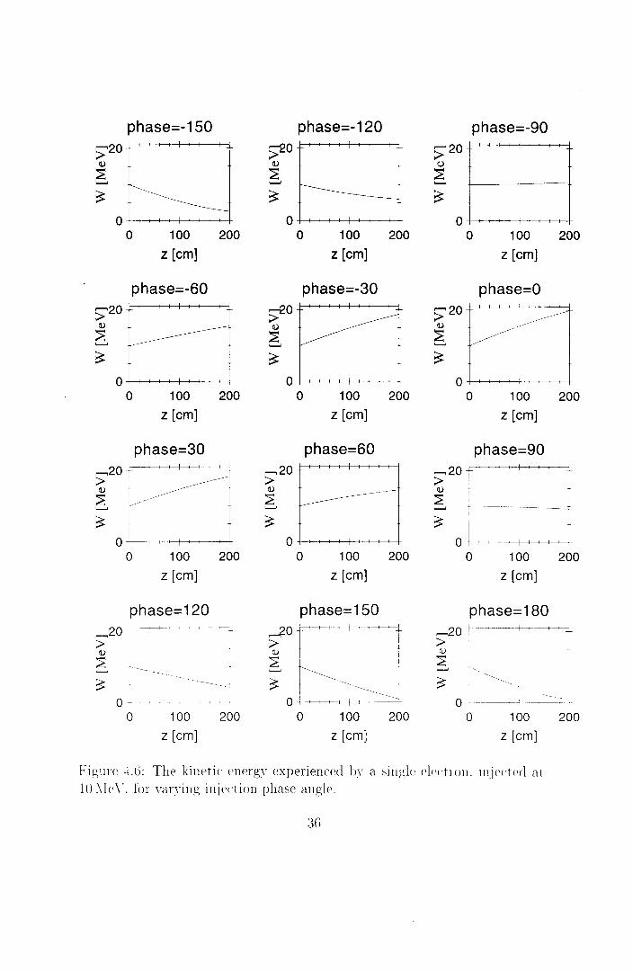
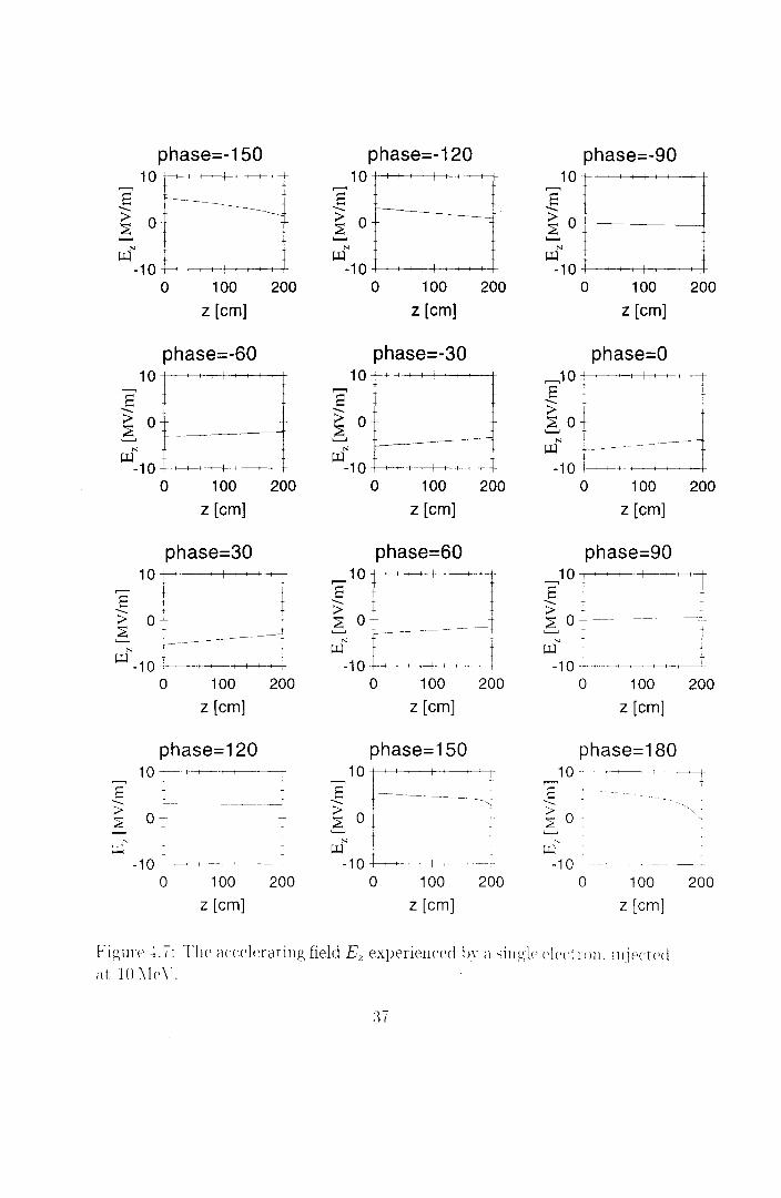
In order to verify the explanation in the previous paragraph, another simulation is carried out, namely fore an electron with W = 10 Me V, which implies f3z ~ 1. Now, cf. figures 4.6 and 4.7, the kinetic energy reaches its maximum of 20 Me V for <P = 0 and the field decay as seen by the electron is as expected from figure 2.10. For <P = 180° the electron is effectively decelerated, but because it slows down too much in the end, it cannot keep up with the wave anymore, so it will not reach zero kinetic energy.

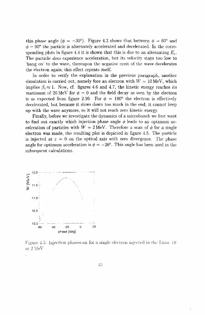
Finally, before we investigate the dynamics of a microbunch we first want to find out exactly which injection phase angle <P leads to an optimum ac­celeration of particles with W = 2 Me V. Therefore a scan of <P for a single electron was made, the resulting plot is depicted in figure 4.5. The partiele is injected at z = 0 on the optical axis with zero divergence. The phase angle for optimum acceleration is <P = -20°. This angle has been used in the subsequent calculations.

12.0 ~~ -~ -~·~~"-~-

> ~ 11.5' //--

~

11.0 -~

10.5-

I 10.0--

·60 -40 -20 0 20

phase [deg]

Figme 4.0: Injection phasescan fora single electrou iujected in th<• Liu;w 10 at 2:\leV

.........,20 > V

6 ~

phase=-150

100 200

z [cm]

phase=-60

100 200

z [cm]

phase=30

I 0 -'---+---+--+--4--+--+--+-+-+

0 100

z [cm]

phase=120

200

.........,20 _,-~.~---~

> V

:E ~

~ 0 -~- --- ---~------

0 100 200

z [cm]

phase=-120

100 200

z [cm]

phase=-30 ~0 V

~ ..........

~ 0

0 100 200

z [cm]

phase=60 .........,20 > V

~ ..........

~ 0

0 100 200

z [cm]

phase=150

tor ··T 6 t~ ~ I ----------------~--------

o -1---+---+---+-- " +----"----+--~ 0 100 200

z [cm]

phase=-90

100 200

z [cm]

phase=O

0 -t--+-----+--+--+--t--+--t---t---+--t

0 100 200

z [cm]

phase=90

.........,20~' ·-~ > . ~ i-- ...... --j

0 ~+--+--t--+-+--+---+-+ 0 100 200

z [cm]

phase=180 .........,20 J ·- 1---+--+--j-+----+--+--c::t­

> V

6 ~

0 --·--~-! ____ .____--:- :_

0 100 200

z [cm]

Figmc -±.6: The kinetic en erg,· experienc<~d by a single electron. inje<'l ed at LO \Ie\'. fm ,·;-nTing injection phase angl<'.

36

phase=-150 10 ,.......,

E -.... > 0 6

N (.l.l

-10 0 100 200

z [cm]

phase=-60 10

s -.... > 0 ~ ..........

N (.l.l

-10 0 100 200

z [cm]

phase=30 ,.....-, 10 i I

E 1 -.... + > o_L 6 ;___--~--~ (.l.l" 1 Ü T . -+-+-+--<----r-- ---,·-----------r-+----+---------r-

I I I

I 0 100 200

z [cm]

phase=120 1 0 --+--+--+--r--r--+---+-~

0-

(.l.l' --1 0 - -~--- -~-·---

0 100 200

z [cm]

phase=-120 10

,......., E -.... > 0 ~ ...__.

N

(.l.l -10

0 100 200

z [cm]

phase=-30 10

,......., E -.... > 0 ~ ..........

N

(.l.l -10

0 100 200

z [cm]

phase=60 1 0 +-+-+--+--+-+~-+-+-+

'E -.... •:;;• 0 I ~ ---j

-1 0 -+--+--+-t-f--+---r-~-+---t-

0 100 200

z [cm]

phase=150 10 1 I 0 r--- --- ~

;J + . -1 0 ~-+--+-+ • ~-· ..•

0 100 200

z [cm]

phase=-90 1 0 -t-+-+-+-+-+--+--+---+---+--+

]" > 0 _j______

~ i ~---------'t' (.l.l .

-1 0 -t--+---+--+--t-+-+--+--+-+-+

0 100 200

z [cm]

phase=O ,......., 1 0 -t--+---+--+--t-+-+-+--+-+-+

E + -.... ~

~ Of ~1 (.l.l 1---

-i--1 0 ~--+-+-+-+--'---+--+-+--+-+

0 100 200

z [cm]

phase=90

]"10---~ ~ > : I 6 ° -=-------~--- ---~t-

N -(.l.l

-10 --+

0 100

z [cm]

phase=180

200

1 0 -· •· -+--~,____,____,-----+

u.f -10 ·-------

0 100 200

z [cm]

Figure 1 ï: Tlw accdnatiug field Ez experieuced lJy ;\ siugl<' clf'c-1 m11. inj<'ct<'d at Hl :\Ie\-.

4.3.2 Bunch Simulations

A limited number N of macroparticles is used for simulating bunch evolution

in the accelerator. The larger N, the more the simulation represents the actual charge distibution and the more accurate the c:alculated parameters

will beo The drawback is that the CPU time for calculations that take space charge into account is approximately proportional to N'2 0 So we have to check for which values of N calculations convergeo In this respect, emittance calculations are the most critical. Figures 408 and 409 lJelow display the final emittances for varying numbers of particleso The GPT element clescribing

10 ........., ;:j

d 8 '--'

w'""

6

4

2

0 100 200 300

N

400

t ----t

500

I t

1

j

Figure 408: Transversal emittance Er at the exit of tlw Linac 10 as a fnnction

of the uumber of macropartic:les No

the hunch c:an only handle fixed numlJers: ;V=70 190 :37, Gl. 91. 1:270 169, :2170 271. .331, 397,0 0 0 0 For N = 7 there is no resul1 lwcause in that <<\SC onho onc of the macro particles fully traverses tlw linaco It is assllltl<'d that <'lltittance calc:ulations are reliable for N 2: 271. In tlw follm,·ing <<lkulations

:271 macro particles represent thc microbunc:h. HaYing performeel all pn'l·ious simula tions. W<' inwstiga t <' tlw 1 H' lu\Yionr

of a 1 ()() pC lmnch in thr liuac. The radial emi tt anc<' f, ( d. figm<' 1.10) grmYs Ir\ st in t he first part of t he accelerator, lwc:a u se of spac<' chmg<' n'pnlsion. [wntualh". most of t he part i des hit tlw wal! or Oll<' of tlH' <·it culm discs

.38

4

2

100 200 300 400

N

500

1

+ ~

I T

l I + I

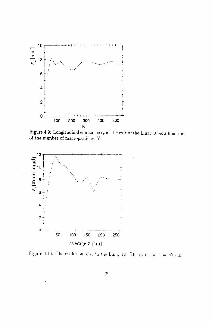
Figure 4.9: Longitudinal emittance Ez at the exit of the Linac 10 as a function of the number of macroparticles N.

I

2_;

1 0

50 100 150 200 250

average z [cm]

Fïgnn• -!.Hl: The e\·olntiun of r, in tlw Lirwc 1(). Tlw <'Xit is <~r ~ =]()()<"lil.

39

of the linac and consequently no Jonger contribute to the emittance. This causes it to be reduced by a considerable amount. The fluctuations inside the linac are probably a consequence of GPT ignoring the vector potential. This means that Behind the linac (z > 200 cm), Er remains constant, as is to be expected. The longitudinal emittance Ez (not depicted) has a z-dependence similar to Er· So also in the longitudinal direction the emittance goes down because particles are lost. The rms bunch length at the linac exit has become very large: approximately llOOfs (starting value: 80fs).

It appears that the accelerating field in the linac is too weak to preserve the size of the microbunch. The next question is: what accelerating field am­plitude is required to let all macroparticles reach the linac exit? And, which amplitude in Ez do weneed to accomplish (or approach) the goals mentioned in chapter 1 (transversal emittance 17r mm.mrad and bunch length 30 J-Lm)? An answer to the first question is given in figure 4.11. The number of parti-

100 .........,

~ ..........

~ 80

z 60 T

I t

40 t I

20 L~~+ 4

0 5 10 15 20 25 30 35

IEzl [MV/m]

Figure 4.11: Fr action of the tot al in i ti al charge that n~acht~~> the exit of the Linac Hl as a func:tion of the average longituclinal elec:tric field.

des reac:hing the exit N' is sc:anned for varying I Ez I, the ayeragr acc:elerating field amplitude. The minimum average field required fm acc:cleration of tlw whole bunch is about IEzl = 30l'viV/rn. whic:h is six times the actual \<Üue ( 5.0:\I\jm) at which the machine presentlv operates. The lmnch parameters at t hr linac exit for this <m~rage field strength are listed in t a hl i' 1.:2.

40

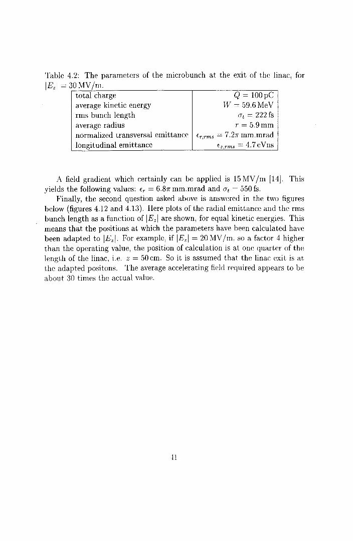
Table 4.2: The parameters of the microbunch at the exit of the linac, for

IEzl = 30 MV /m. total charge average kinetic energy rms bunch length average radius

Q = 100pC W = 59.6MeV

CJt = 222 fs r = 5.9mm

normalized transversal emittance Er,rms = 7.27r mm.mrad longitudinal emittance Ez,rms = 4.7eVns

A field gradient which certainly can be applied is 15 MV /m [14]. This yields the following values: Er = 6.81r mm.mrad and CJt = 550 fs.

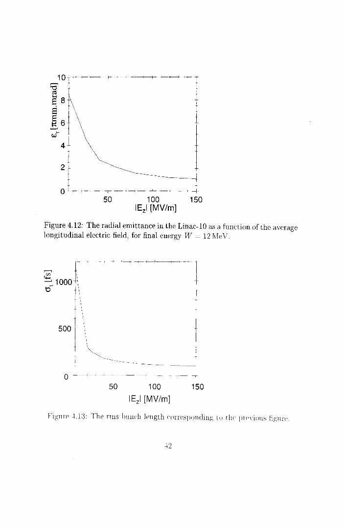
Finally, the second question asked above is answered in the two figures below (figures 4.12 and 4.13). Here plots of the radial emittance and the rms bunch length as a function of IEzl are shown, for equal kinetic energies. This means that the positions at which the parameters have been calculated have been adapted to IEzl· For example, if IEzl = 20 MV /m, soa factor 4 higher than the operating value, the position of calculation is at one quarter of the length of the linac, i.e. z = 50 cm. So it is assumed that the linac exit is at the adapted positons. The average accelerating field required appears to be about 30 times the actual value.

-!1

10~~~~~~~~~~~~

~ ro s 8 s ê6 .........,

w'"'

4

2

50 100 150 IEzl [MV/m]

Figure 4.12: The radial emittance in the Linac-10 as a function of the average longitudinal electric field, for final energy W = 12 Me V.

,---, VJ

~ 1000 b

500

0

t

50 100 150

IE2 1 [MV/m]

Figure -±.13: The rms bunch length conesponding to t he pn·,·ious hgm<'.

-12

4.4 Simulations in the RTME Cavity

As a next structure to be studied we take the accelerating cavity of the Race­track Microtron Eindhoven, as this is readily available in the group FTV. Since it was built to accelerate electron bunches genem,ted and accelerated in the Linac-1 0, the expectation is that its performance w. r. t. the preservation of the bunch parameters is nat as paar as that of the Linac-10. Note: there are na external magnetic fields applied.

4.4.1 Single Partiele Simulations

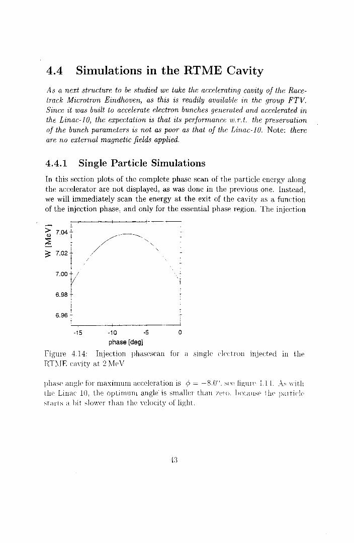
In this section plots of the complete phase scan of the partiele energy along the accelerator are not displayed, as was done in the previous one. Instead, we will immediately scan the energy at the exit of the cavity as a function of the injection phase, and only for the essential phase region. The injection

r-- i

~ 7.o4f ~ ~ ........., I

~ 7.021

7.00t/ i

6.98 +

+ 6.96.:..

-15 -10 -5 0

phase [deg]

Figure 4.14: lr1jection phasescan for a single electrou injected m the TIT~IE cm·ity at 2 Me V

phase angle fór maximum acceleration is r/J = ~8.0". scP figur<' -1.1-J. As with tht~ Linac 10, the optimum angle is smaller than zero. lwcause tlw particl<' stmts a bit sluwer than the velocity of light.

4.4.2 Bunch Simulations

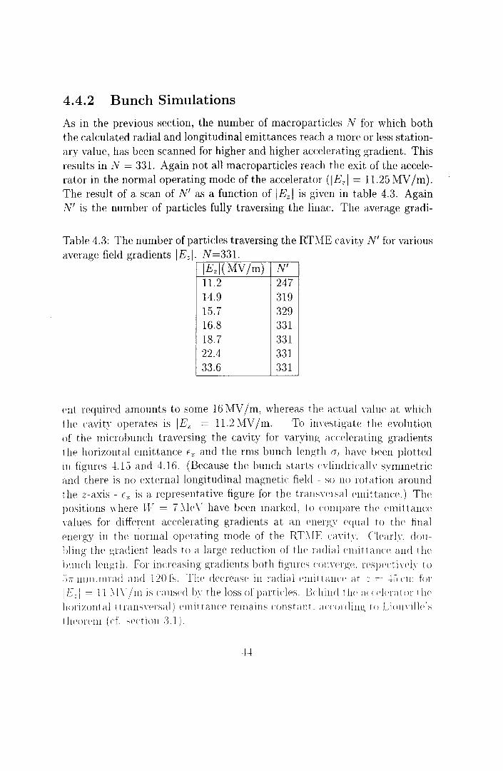
As in the previous section, the number of macroparticles N for which both the calculated radial and longitudinal emittances reach a more or less station­ary value, has been scanned for higherand higher acu~lerating gradient. This results in N = 331. Again not all macroparticles reach the exit of the accele­rator in the normal operating mode of the accelerator (IEzl = 11.25 MV /m). The result of a scan of N' as a function of IEzl is given in table 4.3. Again N' is the number of particles fully traversing the linac. The average gradi-

Table 4.3: The number of particles traversing the RTME cavity N' for various

average field gradients IE z I· N =331. IEzl( MV/m) N' 11.2 247 14.9 319 15.7 329 16.8 331 18.7 331 22.4 331 33.6 331

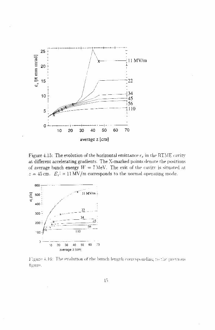
<'nt requirecl amounts to some 16 MV /m, whereas tlw actual value at which the cavity operaJes is IEzl = 11.2 MV /m. To investigate the evolution of the rnicrobunch traversing the cavity for varying au:ch~rating gradients the horizontal emittance fr ancl the rms bunch length (J1 have been plotteel in figures -L 15 and 4.16. (Because the bunch starts cvlindricallv symmetrie and there is no external longitudinal magnetic field - so no rotation armmd the z-axis - E1 is a representa ti ve figure for the tra11swrsal <'mi t tanc:e.) Tlw positions \Yhere TF = 7 :.Ie V have been mar keel, to compare t h<' <~rnittance yalues for different accelerating graclients at an <'ll<'li!,V <'qual to th<' final energy in the normal op<'rating mode of the RT;.,IE ccn·ih·. Cll'arlY. dou­hling the graclient leadstoa large reduction of tlw radial <'mittance and thc 1 lllnch lengt h. Fm incrcasing graclients both figurcs conn't-g<~. n'S]H'c.ti veh· to !11 ntlll.lllrèld ;md 120 fs. Tlw decrease in radial <'tuitt èllH"(' ilt :: = -±.-)ent fm I Cl= 11 '\I\/m is UlllS('d b,· the loss ofparticles. i3<·hind tlw <l<T<'i<'riltm thC' hmizontal 1 tr;msversal) <'mi trance n~mains constant. i\ccmding to Lionvill<'·s tll('Ol<'llt (cf. section :3.1).

1-J

25 i ......., "0 ~ :-E ' 20 ~ E E \=:

15-......... "' w i

10 T I

'

5_;_ I

+ 0

r T I\ ' / \- ---il!MY/m

I I ~------22

t

10 20 30 40 50 60 70

average z [cm]

Figure -:!. 15: The evolution of the horizontal emittance Er: in tlw RT\IE e<t\·itY at different accelerating gradients. The X-marked points denote the positions of average bunch energy W = 7 Me V. The exit of the cavitY is situatrd at z = -!5 cm. IEzl = 11 MV/m corresponds to the normal OIWrating mode.

600

400.:. ~/

/

-':C 11 MV/m-

_,-/

7'1 -x---------~---300- /

200 ~- // _.-)(""'" -=======3=4=;;::·=-1-=5 . x- - 56

1oo fi~C 110

0 ---~-· 10 20 30 40 50 60 70

average z (cm!

figm<' t lG: Thr ('Yolution of dw bunch lengrh ('Oll(':-ijl<Htdiu,ll, r() rIj(' pr<'\"HlllS

hglll'('.

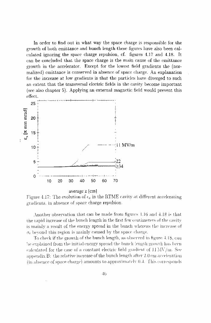
In order to find out in what way the space charge is responsible for the growth of both emittance and bunch length these figures have also been cal­culated ignoring the space charge repulsion, cf. figures 4.17 and 4.18. It can be concluded that the space charge is the main cause of the emittance growth in the accelerator. Except for the lowest field gradients the (nor­malized) emittance is conserved in absence of space charge. An explanation for the increase at low gradients is that the particles have diverged to such an extent that the transversal electric fields in the cavity bec:ome important (see also chapter 5). Applying an external magnetic field would prevent this effect.

' -L

1 I

./ ____ --~11 MV/m

10 20 30 40 50 60 70

average z [cm] Figure 4.17: The evolution of fx in the RTME cavity a.t different accelerating graclients. in absence of space charge repulsion.

Another observation that can be made from figm<~s -J.lG a.nd -±.18 is that the rapiel increase of the bunch length in the first few centimeters of the cavity is mainly a result of the energy spread in the bunch whereas tlw inc:rease of a 1 henmd this region is mainly caused by the space charge.

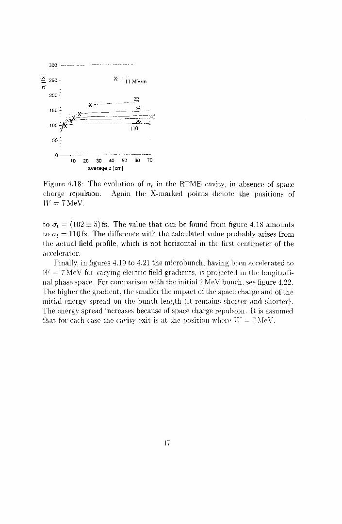
To check if the growth of the bunch length. as ohsern~d in figmc -±.18. eau ])(' cxplainecl from the initial energy spread thc bnnch lcngth grm\"t h has h<~<'Il calcnlatccl for the case of a constant electric field gr<Hli<'lli. of J 1 .\I\" /nt. Sc<' appendix I3: the rel<·ttive increase ofthe bunch lengtlt aft<T :2.0 nu acceleration (in absence of spac:e charge) amounts to approximat<'h· O.l. This <"otT<'sponds

46

300 -------------------·· ----------

x-- 11 MV/m

200-

~----------

150- ____ ]i )E----

-+5 ~~- )0 100 ï·- - ---------110- --_

50 _:_

0--------~-------10 20 30 40 50 60 70

average z (cm]

Figure 4.18: The evolution of CJt in the RTME cavity, in absence of space charge repulsion. Again the X-marked points denote the positions of W = 7MeV.

to CJt = (102 ± 5) fs. The value that can be found from figure 4.18 amounts to CJt = llO fs. The difference with the calculated value probably ar·ises from the actual field profile, which is not horizontal in the first centimeter of the accelerator.

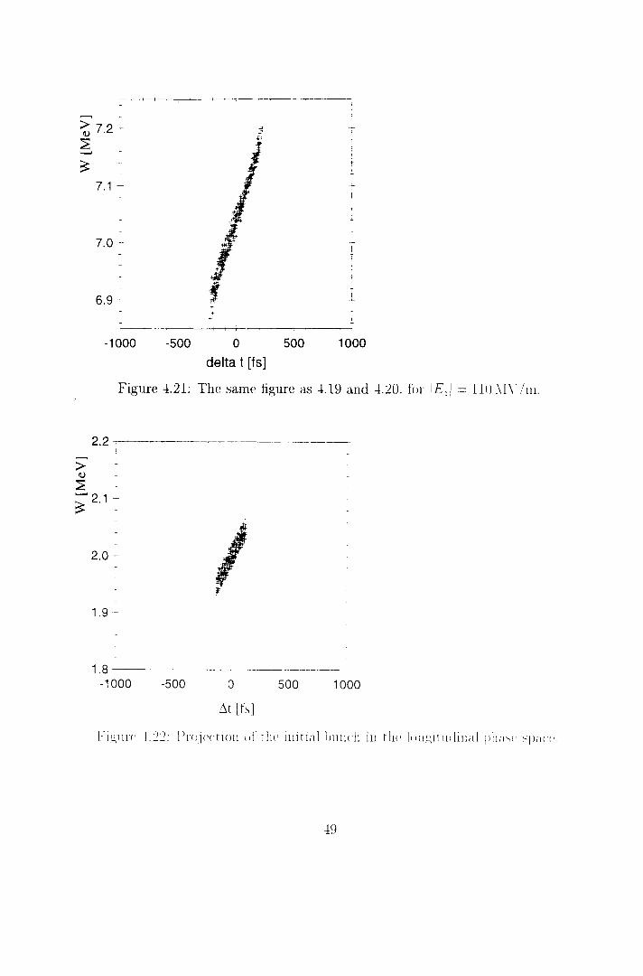
Finally, in figures 4.19 to 4.21 the microbunch, having been ac:celerated to TF = 7 Me V for varying electric field gradients, is projected in the longitucii­ual phase space. For comparison with the initial2 Me V bunch, see figure 4.22. The higher the gradient, the smaller the impact of the space charge and of the in i ti al energy spread on the bunch length (i t remains shorter a nel short er). The energy spread increases because of space charge repulsiou_ It is assumed that for each case the c:avity exit is at the position where TT'= 7 ?\Ie V.

-!ï

I

> l 0 7.2' ~ t ...._..

~

7.0

! T • i

-1000 -500 0 500 1000

delta t [fs]

Figure 4.19: Projection of the bunch in longitudinal phase space. aft<~r ac­celex:atimi to 7MeV by !Ezl = 11 MV/m

- '·.·· '"·. .

T ,__, r ~ 7.2+ ~ ...._..

~ 7.1 ~

l

7.0 ~

6.9-

-1000

' ,+:~-

·~-+...-._­

- -,+..-- =~ __ :"t.

-'t~'Çt--~~ _ ... ~

-500 0 500

delta t [fs]

1000

Fi~l!n' -1.:20: Tlw sametigure as -1.1!). t'or 1E: = ll \[\)111.

48

T

7.1 -;-

7.0 -

6.9-

-1000 -500 0 500 1000

delta t [fs]

Figure -!.21: The same figure as -!.19 and -!.20. for !E:I = 11() .\I\)111.

2.2 .,..-, ------

2.0 - I t

1.9 -

1.8 -----·--~~------- -·--·------------1 000 -500 0 500 1000

i'lt [ fs]

Fi~tllr' L!l: Projeniou l)r rlw iuitial lnllwll iu tlw l<lll!.!,ltlliliu;tl p\tii-,(' "Jl<tl I'

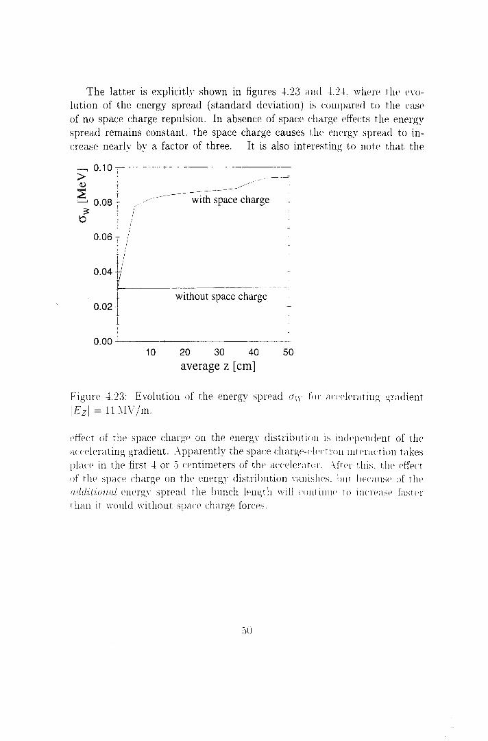
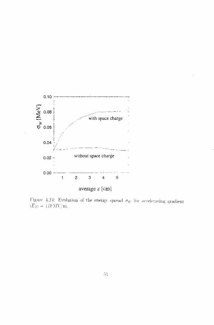
The latter is explicitl\· shown in figures -1.23 awl -1.2-1. wlwre the evo­lntion of the energy spread ( standard deviation) is compan~d to the case of no space charge repulsion. In absence of space charge effects the energy spread remains constant. the space charge causes the energ,y spn~acl to in­crease nearly by a factor of three. It is also interestin~ to note that the

- I 0.06: 1

f

d 0.04 +;

-~ -------~-----------

with space charge

!---------------~--~- ~ -·

0.021 1

10

without space charge

20 30 40 50

average z [cm]

Figure -1.23: Evolution nf the energy sprPad (}1 1· for acn•len\t.ing gradiPnt

IEzl = 11 \IV/m.

effpct of rhe spac:e charge on the energ~· distributim1 is ind<']Wndent of the accelerating gradient. Apparently the span~ charge-<'l<·<·trrlll interaction takes plan• in the first -! or ;] centimeters of tlw acceleratm .. \ft<·r rhis. th<·· effect uf r he span' charge on t he energy distri hn ti on \"itllish<'s. I >1 tr I wc a u se uf r lw rulditunw.l energY sprPad the lmnch lengrh will r·ontillll<' ru incr<"'ase fasrer t lwn i t wonlel without space charge forces.

j()

0.10 •

> 1 ~ 0.08 I

......... ~

b 0.06

I 0.04+.

'I +/

/.~~·space charge

./ /

y,______. ___ - .. -

0.02-

0.00 --·--· 1

without space charge

2 3 4 5

average z [cm]

figme -L:2-L En)[ution of the energv spread a,,. for ;wceleratiug gl<ldiPnt E:-:i = 110 .\I\)m.

4.5 Conclusions

In this chapter single partiele tracking simulations insiele the periodic part of the travelling wave Linac-10 have been performed. It has been shown that the non-propagating terms of the longitudinal electric field, which are relatively large, do not affect the effective energy gain. It is also shown that 2 Me V electrons have to be injected at a phase angle below zero ( -20°) to optimize the energy gain.

After this, bunch simulations have been performed, starting with a check of the convergence of GPT calculations in the Linac-10, which resulted in a required number of macropartieles of 271.

The electric fields in the normal operating mode of the Linac-1 0 are far too low, the bunch is totally spoilt, already in the fi.rst part of the accelerator. For higher accelerating fields the situation quickly improves. Using a achievable field gradient of 15 MV /m , the following bunch parameters are attained: 100pC, Er= 6.81rmm.mrad and at= 550fs at W = 12MeV.

Single partiele tracking simulations performeel in the standing wave RTME cavity show that the optimum injection phase angle for 2 Me V elec­trans amounts to -8°.

A convergence check resulted in 331 as the required number of macropar­tieles.

In the normal operating mode of the RTME cavity (11 MV /m) the follow­ing bunch parameterscan be reached: 75 pC (no coils), f 7• = 5.4 1rmm.mrad and a1. ~ 525 fs at 7 Me V. A maximum applied gradient of three times the normal value ( which is nearly 3 Kilpatrick, seen chapter 5), leads to these val­nes: 100 pC, 1.571' mm.mrad and 200 fs, at 7 Me V. Applying this maximum gradient using 5 accelerating cells yields a final energv of 10.3 IvieV. From fig­ures 4.15 and 4.16 it can be estimated that this leads to f 7 = l.81r rnm.rnrad and a1 ~ 215 fas.

It should be notecl that there is no aclditional drift space taken into ac­count in the calculations in this chapter.

Space charge effects are the main cause of emittancc~ growth. The growth of thc bunchlength is causecl by both the space charge and tlw iuitial energ,· spread.

The spac:e charge causes an increase of the initial cnergy spr<'ad ;mcl does t his mainlY in t he~ first centimeters of the accelerator. Bec a ns<' of t his ad di­l ional erwrgY spread the bun eh length grows fastPr a long t ll<' liuac t han i t wonlel in a bsenc<' of space charge dfects.

:)2

Chapter 5

Microbunch Dynamics in Short Accelerating Structures

5.1 Intro cl uction

In the previous chapter the RTME cavity has been investigated making use of the Fourier coefficients of the axial electric field. These coefficients result from calculations by De Leeuw, see chapter 3. In these calculations the electromagnetic fields and resonant frequencies insiele the total accelerating cavity (including o.ff-axis coupling slots) were found by combining the codes Poisson/Superfish and MAFIA [6]. (This combination was used because, unlike Superfish, MAFIA can be used to calculate electromagnetic fields in structures that are not cvlindrically symmetrie.)

In this chapter short structures that consist of individnal acuMrating and coupling cells of the RT\IE cavity are investigated. B<'<:<ll!se these structures contain one half cell they are inserted in Superfish again. as a whole. Off­axis coupling slots are not implemented, MAFIA lws uot been nsecl. This implies that the electromagnetic fields and resonanc<' fn~qw•ncies n'suiting from Superfish calculations are just an approxima.tion. Because om main interest concerns the magnitude of the longitudinal electric field lH'<-H t he u!Yit\· axis, this is not a problem however.

5.1.1 Superfish

SnJH'rfish is a 2D computer code, that can he used to r'idculat<' cYiiwlriudiY sYmmetrie elcctromagnetic field moeles in standing w;n·r· st met 1\l'<'S. It so!Yf's

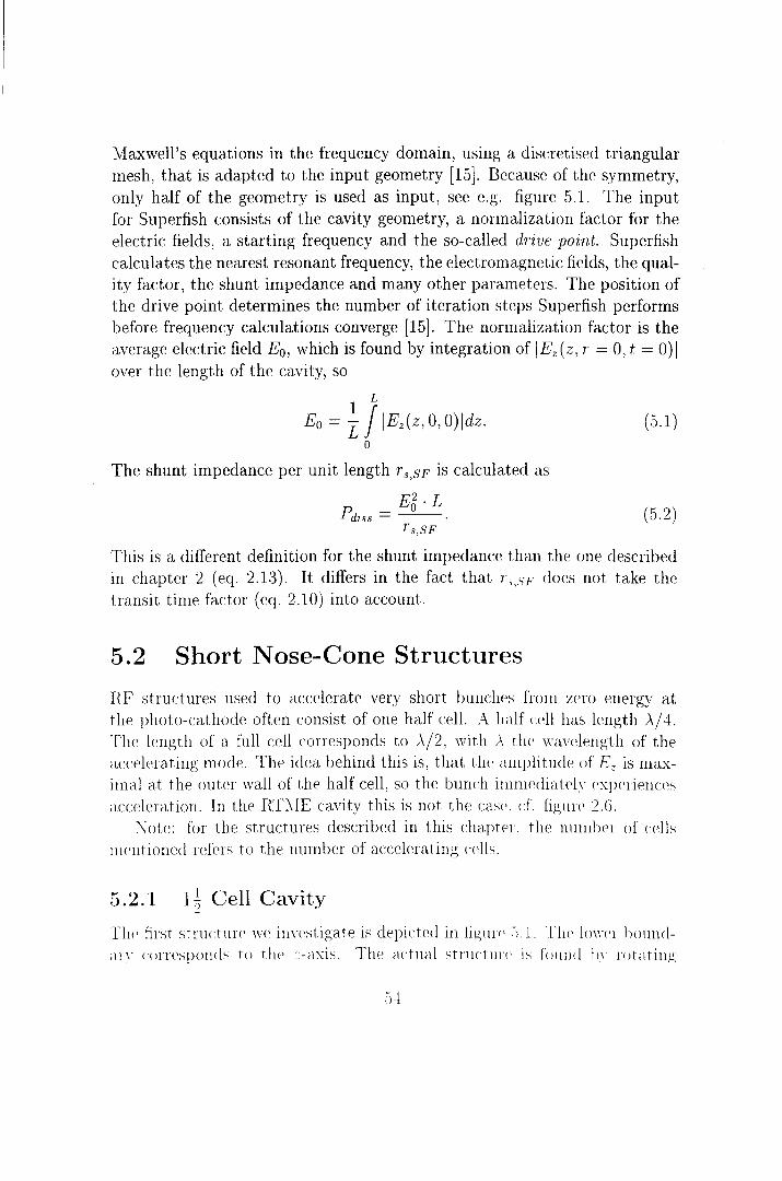
Maxwell's equations in the frequency domain, using a discretised triangular mesh, that is adapted to the input geometry [15]. Because of the symmetry, only half of the geometry is used as input, see e.g. figure 5.1. The input for Superfish consists of the cavity geometry, a normalization factor for the electric fields, a starting frequency and the so-called drive point. Superfish calculates the nearest resonant frequency, the electromagnetic fields, the qual­ity factor, the shunt impedance and many other parameters. The position of the drive point determines the number of iteration steps Superfish performs before frequency calculations converge [15]. The normalization factor is the average electric field E0 , which is found by integration of IEz(z, r = 0, t = O)l over the length of the cavity, so

1 L

Eo = L j IEz(z, 0, O)idz. 0

The shunt impedance per unit length rs,SF is calculated as

E2. L Pdiss = - 0

-. Ts,SF

(5.1)

(5.2)

This is a different definition for the shunt impedance than the one described in chapter 2 (eq. 2.13). It differs in the fact that r,,sF does not take the transit time factor (eq. 2.10) into account.

5.2 Short Nose-Cone Structures

RF structures used to accelerate very short bunches from zero energy at the photo-cathode aften consist of one half cell. A half <·dl has length )../ 4. The length of a full cell corresponds to )../2, with À th<' wavelengtil of the accderating mode. The idea bebind this is, that the amplitude of Ez is max­imal at the outer wal! of the half cell, so the bunc:h ilnm<~diat<'h· experienccs accderation. In the RT\IE cavity this is not thc cas<'. cf. figm<' 2.6.

~ote: for the structures described in this chaptrr. thc lmmlwr of cclls mentioned rcfers to the number of accelerat.ing cells.

5.2.1 1 ~ Cell Cavity

The first structure we inn•stigate is depictcd in figm<' .-J.l. Th<' lomT honnd­i\1\. conespouds to tlw ><lxis. Thr ;H·tnal strnc1l!l(' is fonnd ]l\· roL1ting

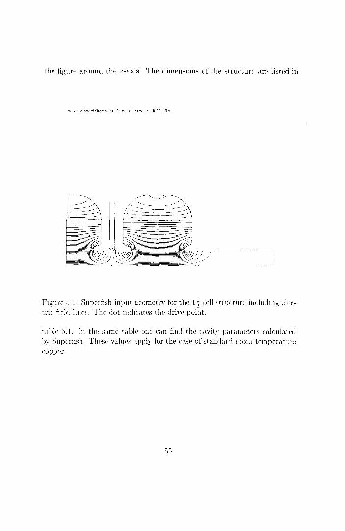
the figure around the z-axis. The dimensions of the structure are listeel in

halve e;ndce!/koppelcel/eindcel Freq = 3011.4q5

Figurc 5.1: Superfish input geometry for the q cell stmc:tme including elec­tric field lines. The dot indicates the drive point.

ta ble :J .1. In the same table one can fin cl the cavi tï parameters calculated hï Superfish. These valnes apply for the case of standani room-temperature copper.

·)·)

J ust like for the RTME cavity, the mode that is nsed for accelerating particles is the ~ mode. There is no effort made to exactly tune the cavity at the frequency required (2998 MHz), because the field lines in figure 5.1 indicate this is the right mode.

Table 5.1: Parameters of the q cell geometry and results of Superfish cal­culations

full cavity length 120.0mm half accelerating cell length 25.0mm accelerating cell length 50.0mm accelerating cells radius 38.5 mm coupling celllength 2.8mm coupling cell radius 35.0mm beam line radius 8.0mm average accelerating field E 0 = 22.00 MV /m

resonant frequency .f~ = 3011.5 MHz quality factor Q = 17.3 . 10•3

power dissipation Prüss = 0. 711 MW stared energy u= 0.651 J shunt impedance per unit length r,,sp = 81.7 MO/m maximum electric field on cavity wall Ez,max = 143 i"v1V /m = 3.06 Kilpatriek

The average axial electric field that is used bas heen adjusted to the maximum value at the cavity wall Ez,ma.r such that it amonnts to three times the so-called Kilpatriek limit. This limit is calculated by Superfish using an empirica! formula that relates the breakdown electric field to the resonant frequency. This formula was introduced over 40 yenxs ago. Nowadays with better vacuum systems and cleaner surfaces it is possible to apply fields well over 2 Kilpatriek [16]. The power dissipated for Ez.max = .3 Kilpatriek still is onlv a fraction of the 10 MW available from our klvstron. The elcctric field profile in the 1 ~ cell structure is depicted in figure ::J. :2.

öG

60~----~-----r----~------~----~-----,

~0~----~----_.----~------._----~----~ 0 2 4 6 8 10 12

z [cm]

Figure 5.2: Electric field profile on the cavity-axis.

Single partiele calculations ( which will not be shown he re) lf~ad to an optimum injection phase angle cPmax = -22°. The conesponding energy gain amounts to 6. W = 2.15 Me V. The transit time factor can be calc:ulated using

T = 6.vV E0 L cos cjJ

(5.3)

This vielels T = 0.87. Scanning the number of macroparticles JV gives con­verging emittances for N = 271, a number which has been used for the su bsequent calculations.

In figure 5.3 the evolution of the buneh length (nns) a1 in th<::~ cavitv (injection at cPmax) is depicted. At the exit of the nn·ity a1 has increasecl Iw a factor of three. Figure 3.4 shows the evolution of the horizontal cmittance. which in turn is increased bv about 80 %.

OI

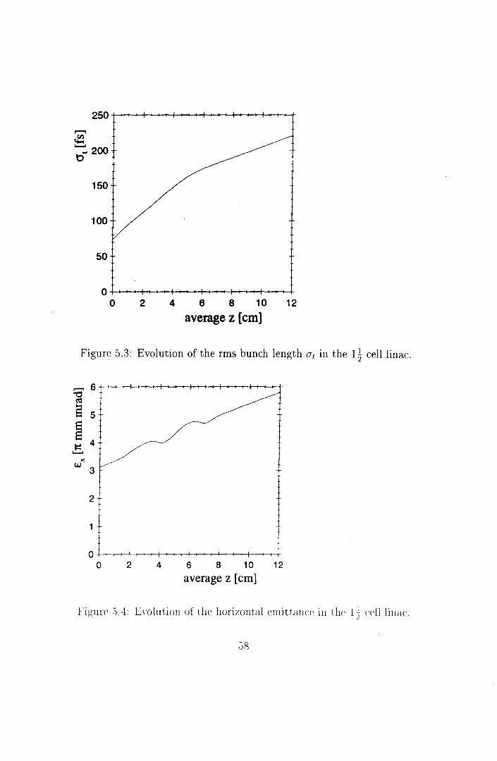
150

100

50

0+---~~--~~~~~~--~~~

0 2 4 6 8 10 12

average z [cm]

Figure 5.3: Evolution of the rms bunch length CJt in the q celllinac.

,........, 6 "0 ('j

8 5 s s

4 ~ ..........

>< w 3

2

o++--~~~~~~--~~~~~~

0 2 4 6 8 10 12

average z [cm]

Figure 5.4: E\·olution of the horizontal ernittance in tlw 1 ± cel! linac.

G8

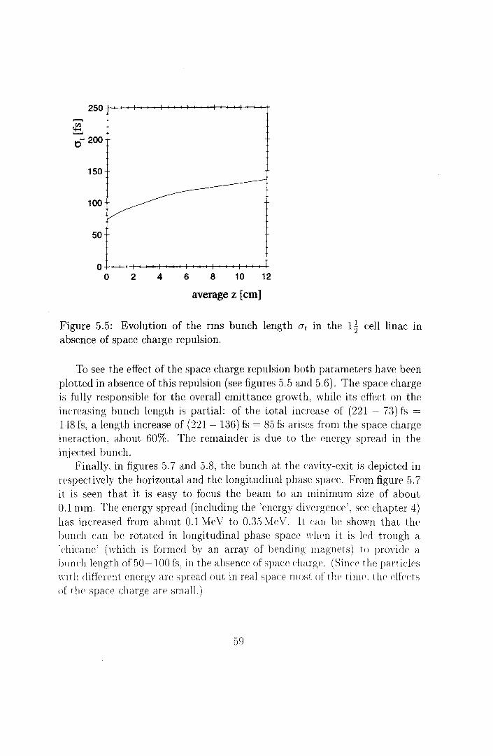
t;;200

150

100

50

o++~~~~--~~~~++~~-+

0 2 4 6 8 10 12

average z [cm]

Figure 5.5: Evolution of the rms bunch length at m the 1 ~ cell linac in absence of space charge repulsion.

To see the effect of the space charge repulsion both parameters have been plotteel in absence ofthis repulsion (see figures 5.5 and 5.6). The space charge is fully responsible for the overall emittance growth, while its effect on the increasing bunch length is partial: of the total increase of (221 - 73) fs =

1-18 fs, a length increase of (221 - 136) fs = 85 fs arises frorn the space charge ineraction, about 60%. The remainder is due to the erwrgy spread in the injected bunch.

Finally, in figures 5. 7 and 5.8, the bunch at the c:avity-exit is depicted in respectively the horizontal and the longitudinal phase space. From figure 5. 7 it is seen that it is easy to focus the beam to an minimum size of about 0.1 mm. The energy spread (including the 'energy divergence', see chapter 4) has increased from about 0.1 MeV to 0.35l'vieV. It eau be shown that the bunch c:an be rotateel in longitudinal phasc space when it is bl trough a "chicane' (which is formeel by an array of bending magnets) to prm·idc a lmnch lengthof 50-100 fs, in the absence of spac:e charge. (Since the particles ,,.i t h different energy are spread out in re al space most of t lH' ti me. t he effects of t he space charge are small.)

59

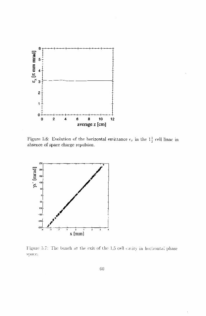
,....., ~ 8 5

ê 4 .!:. o{ 3 r----------------:!.

2

o~~-r~~~~++---r~~~~

0 2 4 6 8 10 12

average z [cm]

Figure 5.6: Evolution of the horizontal emittance fx in the 1 ~ cell linac in absence of space charge repulsion.

250 + ,........,

// '"Ó 200

(1:$

ä 150

.......... 100

~ 50

0

;/ -50

-100

-150

*' -200 , .. -250 1-

-4 -3 -2 -1

x [mm]

figme :J.ï: The bunch at tlw exit of tlw 1,5 cell <<1\·itY in horizontal phase Sjl<lC:C.

GO

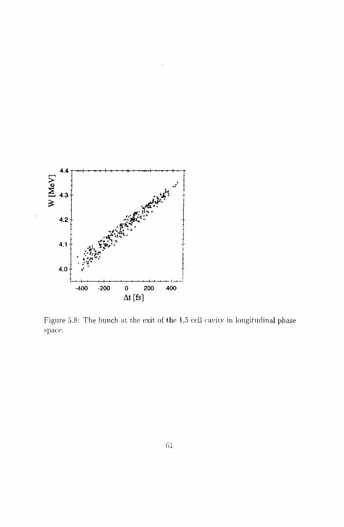
4.4 ,......, > ~

~ 4.3 .........

~

4.2

4.1

4.0

-400 -200 0 200 400

Ll.t [fs]

Figure 5.8: The bunch at the exit of the 1,5 cell cavity in longitudinal phase space.

Gl

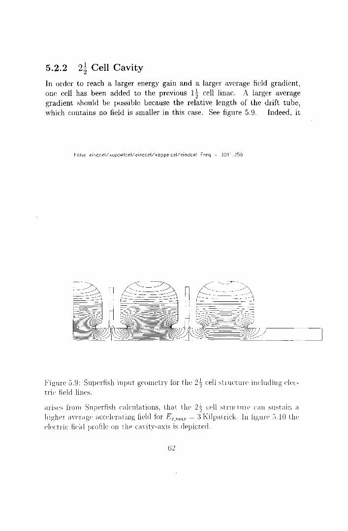
5.2.2 2~ Cell Cavity

In order to reach a larger energy gain and a larger average field gradient, one cell has been added to the previous 1 ~ cell linac. A larger average gradient should be possible because the relative length of the drift tube, which contains no field is smaller in this case. See figure 5.9. Indeed, it

halve eindcellkoppelcel/eindcel/koppelcel/eindcel Freq 3011.356

Figure 5.9: Superfish input geometry for the 2~ cel! stmcture iuducling clec­tric field lincs.

ariscs from Superfish calculations 1 that thc 2~ cel! s1mctmc can sustain a higher awrar-;e ac:celerating field for Ez,nw1 = 3 Kilpatriek In figmc ö.lO the dc~c:tric field profile on t he cavitv-axis is depic:ted.

62

Table 5.2: Parameters of the 2~ cell geometry and results of Superfish cal­culations.

full cavity length 172.8mm half accelerating cell length 25.0mm accelerating cell length 50.0mm accelerating cells radius 38.5mm coupling celllength 2.8mm coupling cell radius 35.0mm drift tube radius R3 = 8.0mm average accelerating field Eo = 25.3 MV /m

resonant frequency .f1 = 3011.4 MHz quality factor Q = 17.6. 103

power dissipation Pdiss = 1.169 MW stored energy u= 1.085 J shunt impedance per unit length Ts,SF = 94.6 MS1/m maximum electric field on cavity wall Ez,max = 143 MV /m = 3.06 Kilpatriek

0 !!. 20

~ 0

-20

-40

-60 -l--+--+--+--t---+--<---+--r~.-t-+~+-+-~---+--+---+--r+--+-<-t--+~+-+--'-0 2 4 6 8 10 12 14 16

z [cm]

Figure S.10: Electric field profile on tlH' cavit,·-axis.

63

For this structure again c/Jmax ~ -22°. The conesponding energy gain is ~ W = 3.51 Me V. Using eq. 5.3 we arrive again at a transit time factor of

T = 0.87.

Ö200

150

100

50

O+rH4~~~+-~~~~~++~~~

0 2 4 6 8 10 12 14 16

average z [cm]

Figure 5.11: Evolution of the rms bunch length at in the 2~ celllinae. The lower curve corresponds to the case of no space charge effects.

The evohltion of the buneh length is depieted in figure 5.11, both for the case of zero space charge and spaee charge 100 pC. The rrns bun eh length increases to 236 fs along the linac, an increase of 163 fs, of whieh about 60% is c:aused by spacc charge rcpulsion. The fact that this percentage does not differ frorn the case of 1 ~ seems to be consistent with tlw observation made in chapter 4. There it is concluded that the electron-space charge interaction takes place in the first centimeters of the cavity. So tlw initia! mwrgy spread and tlw space charge can both be regarcled as starting effects.

In tigure 5.12 the horizontal emittance for both cases is plottül. Between ,z = 0 and :: = 11 cm thc plots are very similar to the si tua ti on of 11 c:ell ( cf. figmc 5.4). as can he expectccl. But between z = 11 c1 u and :: = 14 cm thcre is a sudden increase of f 1 . even in the case of zero space charge! A possihle ('Xplanation fm this could be the that tbc infiuencc of thc tm.nsvf:rsol elcctric tic ld Er on the emi t tance becomrs notica ble if t he a\'('t'agc radius of t he

64

4

2

o++~~~++~~++~~~++~~++~

0 2 4 6 8 10 12 14 16 average z [cm]

FigurP .5.12: Evolution of the horizontal emittance f, in the 21 cell linac. The lower curve corresponds to the case of no space charge efi'ects.

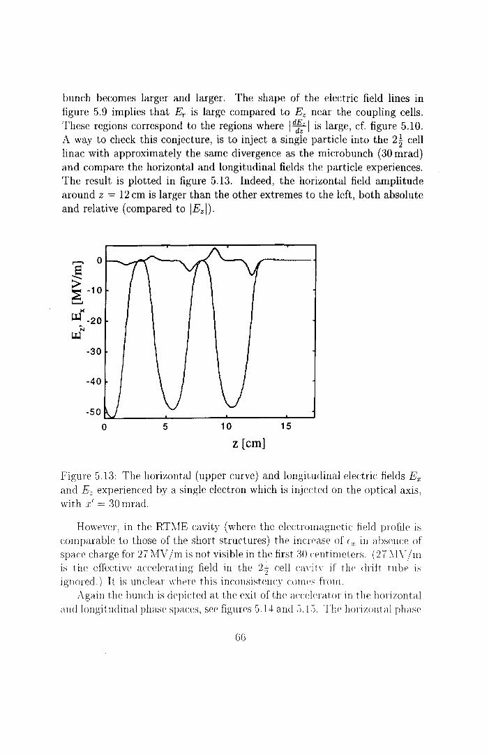
bunch becomes larger and larger. The shape of the electric field lines in figure 5.9 implies that Er is large compared to Ez near the coupling cells. These regions correspond to the regions where 1~1 is large, cf. figure 5.10. A way to check this conjecture, is to inject a single partiele into the 2~ cell linac with approximately the same divergence as the microbunch (30 mrad) and compare the horizontal and longitudinal fields the partiele experiences. The result is plotted in figure 5.13. Indeed, the horizontal field amplitude around z = 12 cm is larger than the other extremes to the left, both absolute and relative (compared to IEzl).

,.._, 0

~ :E -10 ..........

~

~ -20 ~N

-30

-40

5 10 15

z [cm]

Figure 5.13: The horizontal (up per curve) and longitudinal rlectric fields Ex and Ez experienced by a single electron which is injected on the optical axis, with :r:' = 30 mrad.

However, in the RT~IE cavity ( where the electromagnctic field profile is comparable to those of the short structures) the increase of f 1 in absence of space charge for 27?v1V /m is not visible in the first 30 centimeters. (27 :\IV/ m is tlw effec:tive accdcrating field in tlw 2~ cell cm·it1· if the drift tube is ignored.) It is unclear where this inconsistency comcs from.

Again the bunch is depicted at the exit of the accelerator in t he horizontal and longi tudinal phase spa.ces, see figures 5.14 a nel 5.1 :). Thr horizont al ph a se

GG

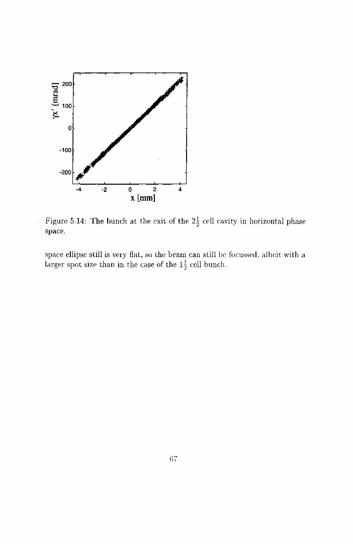
.......... 200

~ ........ 100

~ 0

-100

-4 -2 0 2 4

x [mm]

Figure 5.14: The bunch at the exit of the 2~ cell cavity in horizontal phase space.

space ellipse still is very flat, so the beam can still be focussed, albeit with a larger spot size than in the case of the 1 ~ cell bunch.

G7

,.....,

~ 5.7 ........

~ 5.6

5.5

5.4

-400 -200 0

~t [fs]

+

200 400

Figure 5.15: The bunch at the exit of the 2~ cell cavity in longitudinal phase spacc.

68

From figures 5.8 and 5.15 it can be seen that the energy spread does not increase any further, while traversing the second accelerating cell. This again confirms that the space charge interaction is restricted to the first part of the linac.

5.3 Conclusions

In this chapter two 'nose-cone' structures haven been investigated, a 1 ~ cell cavity and a 2~ cell cavity. It has been investigated which final kinetic energy gain can be reached by 2 Me V electrons, where it has been assumed that the field breakdown limit is 3 Kilpatriek For the 1 ~ cell structure this yields W = 4.2 Me V, for the 2~ cell structure W = 5.5 Me V can be attained.

The parameters for the 4.2 Me V bunch are a radial emittance of l.57r mm · mrad, _:fi a rms bunch length of 221 fs and a energy spread of about 15%. For the 5.5 Me V bunch the results are 225 fs, 2.57f mm · mrad and an energy spread of about 10%.

To reach an energy gain ~W = 8 Me V we woulel need at least 5~ accel­erating cells.

In both structures, the evolution of the bunch length is similar to the comparable case in the RTME cavity. Apparently the field levels that can be reached in the first half cell are not sufficient to actually decrease the initial bunch length growth.

In the 2~ cell cavity it is found that the emittance increases in the final cell in absence of space charge. This might be caused by the transversal dectric field, but this is not consistent with the emittance evolution in the RTME cavity (see chapter 4).

Comparing the 2~ cell nose-cone structure with the Brookhaven-type structure (as designed by Van der Geer ancl De Loos [17] (cf. table5.3) shows that the shunt impedance and the quality factor of the nose-cone structure are larger. So the nose-cone structure uses its power more dficiently than the Brookhanm-type. But, hec:ause of its geometry (see figme 1.1), the latter has rdatiwlv small maximum electrit fields on its houwlari<'s and so can withstand higher accelerating fields.

G9

Table 5.3: Parameters of the 2~ cell Brookhaven-type cavity

resonant frequency cavity length stored energy power dissipation quality factor shunt impedance per unit length transit time factor maximum electric field on cavity wall energy gain 2 Me V electrous

70

.f"' = 2998.2 MHz 0.200m

u= 7.408 J Pdiss = 10.363 MW

q = 13.5. 103

r,,sF = 71.8 Mnjm T = 0.62

Ez,max = 131 MV /m = 2.81 Kilp. ~Hl= 7.4MeV

Chapter 6

Concluding Remarks

In this graduation project the dynamic behaviour has been investigated of 2 Me V, 100 pC electron microbunches in the travelling wave Linac-10, the standing wave 'nose-cone' RTME cavity and two 'nose-cone' structures con­taining one half cell. The main goal was to determine to what extent it is possible to preserve the main parameters of the bunch during acceleration to about 10 Me V (starting values: Er = 0.8 1r mm.mrad, bunch length (rms) CJt = 73 fs, ~; = 2%).

It can be concluded that the travelling wave Linac-10 is not suitable for these demands by far, both because of its length and because of the modest field levels that can be applied.

In comparison to nose-cone structures containing only full accelerating cells, using nose-cone structures starting with one half accelerating cell does notlead to any noticeable improverneut concerni~Zt~l~Je~h growth, which mainly takes place in the first centimeter:of.the acceleralors. A struc­ture that can deliver thc re~uired 8 Me V energy gain would consis~of 5 full accelerating cells. The~~arameters than c:an be accomplished are fr = 1.87r rnrn.rnrad and CJt :::::::; 215 fs.

In general, the various sirnulations lead to the condusion that the spac:e charge interaction only occurs in the first centimeters of acceleration. Two phenomena are rcsponsiblc for overall bunc:h length growth: the initial energy spread and the space charge interaction.

Finallv. it is concluded that the 1Brookhawn-tvpe' stmc:ture can produce larger graclients than the nosc-cone type, hut at the <'XJWilS<' of Hlllc:h larg<~r

RF power. The shunt impcdanee ancl the quality factor of the nosf'-c:one structure are significant h· higher.

71

Bibliography

[1] M.J. de Loos, S.B. van der Geer, Pulsar Physics; J.I.M. Botman, O.J. Luiten, M.J. van der Wiel, Eindhoven University of Technology, Produc­tion of ultra-short, high charge, low emittance electron bunches using a 1 GV /m DG gun, PAC '99, http:/ jwww.pulsar.nljtuejpac99/pac99.htm (1999)

[2] K. Batchelor et al., Brookhaven National Laboratory, Performance of the Braakhaven Photocathode RF Gun, Nuclear Instruments and Meth­ocis in Physics Research A318 pp. 372-3761 North-Holland (1998)__}

__.__...,. .... -------··---··""·.........,.,..·· ~-"

[3] ;J.D. Jackson, Classica[ Electrodynamics':John ons Inc., New iL 11..

~9~-~! ......... , .. --------- --·---·---~ ~~---, [4] G.A. W~bers, Design of an Electron-optica[ System for a 75 Me V Race­

track Microtron, Ph.D. Thesis, Eindhoven University of Tf~chnology (1994) ---- -

[5] R.W. de Leeuw, J.E. Copppens, Linear Standing Wave Accelerators in the Gigahertz Regime, Tijdschrift van het Nederlandse Electronica- en Radiogenootschap, vol. 59, no. 4, --~iEi!:o~ersiQ_oLThclu:!.~!og:y __ (1994) --

[6] R.vV. de Leeuw, The Accelerator Injection Chain of thc Electron Storage Ring EUTERPE, Ph.D. Thesis, Eindhoven University of Technology (1996)

[ï] ~I. Tceuwcn. The Accelem,ting Cavdy of the Rw:r:tm.d: M-ir:mtron of thc I TE U FEL ProJect. ~I. Sc. Thesis, Eindhon~n Lui wrsitv of T(~chuolog,­(1991)

72

IL \ivtJ .

[8] J.P. PruiksCa, Ele~tromagnetic Fields in Periodically Disk-loaded Cir­cular Waveguides, M.Sc. Thesis, Eindhoven University of Technology (1996)

[9] J .E. Coppens, Design Study for the Accelerating Cavity of the Racetrack Microtron Eindhoven, M.Sc. Thesis, Eindhoven University of Technol­ogy (1994)

[10] A.F.J. Hammen, Partiele Dynamics in the 10 Me V TUE Electron Linac, M.Sc. Thesis, Eindhoven University of Technology (1997)

[11] M. Conte, W.W. MacKay, An Introduetion to the Physics of Partiele Accelerators, World Scientific, London (1991)

[12] M.J. de Loos, S.B. van der Geer, Pulsar Physics, Utrecht, General Par­tiele Tracer - A 3D code for accelerator and beamline design, Proc. of the EPAC'98 _sonf., Stockholm, Sweden (1998) pp. 1245

[13] M.J. de Loos, S.B. van der Geer, Pulsar Physics, Utrecht, GPT User Manual, Pulsar Physics (1997)

[14] T. Shirai et al., Performance of the 100 Me V Injector Linac for the Electron Starage Ring at Kyoto University, Proc. XVIII Int. Lin. Acc. Conf., CERN 96-07 (1996), p. 240

[15] M.T. Menzel and H.K. Stokes, User's Guide jor the Poisson/Superjish Group of Codes, Los Alamos National Laboratory, Los Alamos (1987)

[16] T.P. \Vangler, RF Linear Accelerators, John \Viley & Sans lnc., New York (1998)

[17] M.J. de Loos, S.B. van der Geer, Pulsar Physics, Dt:sign of the TUE Photo-cathode, March 4 1999, internat report (1999)

73

Appendix A

The _ëccelerating field in the modeled Linac 10 ~

The electric field in the Linac 10 is described by eq. 2.20, using the Fourierco­efficients in table 2.5. The zerothorder term describes the propagating term; all higher order terms describe refiections in the linac. Figures 4.4 and 4. 7 only show the zeroth order terms of Ez (as experienced by the electron for various injection phases). In figure A.1, the electric fields that would be ex­perienced by the electron in absence of the zeroth order term, are depicted. The total electric fields combining the zeroth and higher order terms are de­pictecl in figure A.2 ancl clearly are found by superposition of respective plots in figure 4.4 and figure A.l. The electric fielcls have been split in zeroth and higher order terms for reasous of comprehension. Thc dfect of the higher order terms on the energy gain of the electron is virtually negligible, as can he seen by camparing figure A.3 to figure 4.3, ancl the explanation in subsec­tion 4.3.1 is more understanclable if we ignore the oscillatory behaviour of Ez. So, clespite of the large field oscillations caused by the refiec:tions in the linac, tlw effect i ve field can be treated as non-oscillatmv because the increments and decrements of the partiele energy on the partiele en(~rg~' cancel out.

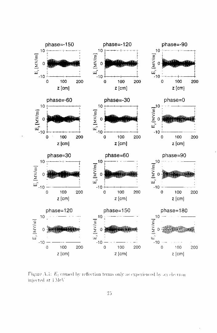
phase=-150 phase=-120 phase=-90 10 : 10 10

T ........, E t E ~

....... I ....... ' > 0 > 0 > 0 ~ ~ ~ ..__.. ' ..__.. ..__..

.... l "

,... T LLl ' + LLl LLl

-10 : -10 ' -10 ' 0 100 200 0 100 200 0 100 200

z [cm] z [cm] z [cm]

phase=-60 phase=-30 phase=O 10 1 ~

10 ........,10~ ........, ~ E E ' ....... ....... > > 0 > 0 ~ 0 ~ ~ ..__.. ...... ..__..

"' T N N LLl t

LLl LLl -10 T -10 -10 0 100 200 0 100 200 0 100 200

z [cm] z [cm] z [cm]

phase=30 phase=60 phase=90 10 I 10 ,_10

........, E ~ ,.... ...::::: ,.... .......

...:::: > > > o· ~ 0 ~ 0 ~ ..__.. '---

,.. .... .... - LLl LLl

LLl --10 I -10 -10

0 100 200 0 100 200 0 100 200 z [cm] z [cm] z [cm]

phase=120 phase=150 phase=180 10- 10 1 0 --- --~------

,_ -~ E

,.... ,.... ....... ....... --> 0 > 0 :::: 0: ~ 2 ~ -

' " ' L:..l LLl Ll..l

-10 -10 -10 ---- - ~~ --- ------·- .

0 100 200 0 100 200 0 100

z [cm] z [cm] z [cm]

Fi.u,un' A.l: E: <<l!lsed In· retlection t<'nus llnh· ;1s <'X])('!Ï<'ll<·<·d In· ;111 <'l<'< rt<Hl

iliJ<'<·t<'d at l .\1<'\.

200

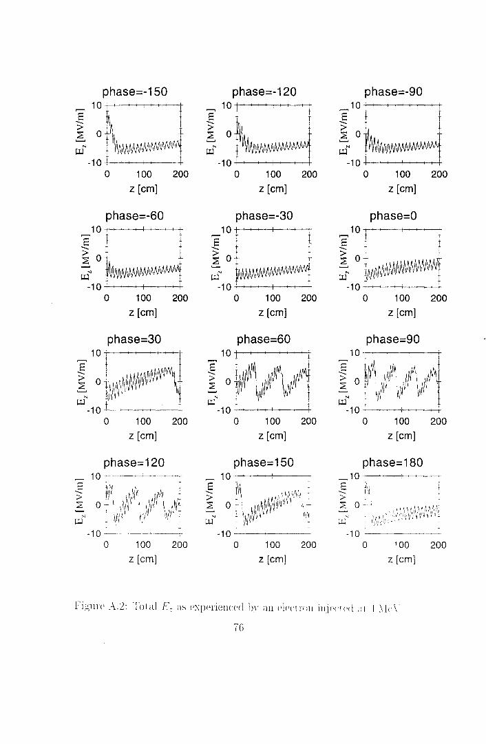
phase=-150 ......., E ..._ > ~

10+1 I I I I t 1

..........

~N t -1 0 -:--: ~--+----+--+->----+--+---+

0 100

z [cm]

phase=-60

200

1 0 f-.-->-+----+---1---+--+---+---+-+

E' ..._

~ 0 ..........

N

~ -1 0 -t-+--+-+--+-t---+----+--+--+-+

0 100

z [cm]

phase=30 10 t

......., + E ~ ..._ l

~ o~WN\

200

~ I

-1 0 -'--r ~--+------+---+---+----+-+-+-+ 0 100 200

z [cm]

phase=120

phase=-120 1 0 +-+---+----+---+-+-+-+---+-+-+ ,...., t

E r ..._ > ~ 0 .......... ~N

-1 0 -t-+--+-+---+-+-+-+--+-+-+

0 100 200

z [cm]

phase=-30 1 0 f-.--+-+----+-+~-+-+-+ ,....,

E ........ t ~ 0

+

.......... N

~ -1 0 -t-+--+-+----+--+-+-+-+--r

0 100 200

z [cm]

phase=60 10 . ~

E L~ .~1: t

; o~~~ ~VI ~ -10 : :

0 100 200

z [cm]

phase=150

76

100

z [cm] 200

phase=-90 1 0 _,_· -+--+--+-+-+--t---+----+--+--+

E' ~ ........

~ 0 .......... ~N

-1 0 -t-+--+-+--+-t--+---+---+-+-+

0 100 200

z [cm]

phase=O 1 0 +-' -+--+---+-----+-----+--+-+---+----+

,...., t E I

> l ~0~

-1 0 -t-+---+---.----+----+-~-+-+-+-0 100 200

z [cm]

phase=90 10- • .

E' i.~M ~~ ~M i > 0 ~~ 1 IN ,J\11 i \IV t

~ " • 1\h 11•1 \,Nï - \N' ,~1 vv

~" I' -1 0 ~--+-i--+-+------+

0 100

z [cm]

phase=180

200

- 1 0 -~-----'--+-+--"-

E t11 > •i

2 0---j

-10 ---~--. 0 100 200

z [cm]

phase=-150

100 200 z [cm]

phase=-60

100 200 z [cm]

phase=30

100 200 z [cm]

phase=120 I 1 t ,.......,1Q+

> l (!) '

~ t I ~ i

atv~ 0 100 200

z [cm]

phase=-120

100 200 z [cm]

phase=-30

100 200 z [cm]

phase=60

100 200 z [cm]

phase=150

0 -t-"4--+---+--+-i-_.__,_~_,..-=-r. 0 100 200

z [cm]

phase=-90

100 200 z [cm]

phase=O

100 200 z [cm]

phase=90

100 200 z [cm]

phase=180 ,.......,10-'-~ '

~ '-'

~ 0 "-.~~~~~

0 100 200 z [cm]

Fip,ure .\.3: Kinectic energy vV in absence of the refi<'<"ting tPllllS in r.lw E:-field as experienced bv an Plectron injected at 1 .\Ie\·.

77

Appendix B

Calculation of Bunch Length Growth in an Electrostatic Field.

In this appendix the increase of the length microbunch ( described in table 4.1) in the first 2.0 cm of the RTME cavity is calculated fora constant accelerating gradient of 11 MV /m. This increase is caused by the initial energy spread. All veloeities mentioned below are oriented in the longitudinal direction.

Consicier two positions in the bunch, cf. figure 4.2: (.0.t,W) = (-120fs,l.95MeV) and (~t,W) = (115fs,2.05MeV). Let us denote these points as A and B. The initial elistance between both points is 1 ~ c · 335 fs. The length growth ~~is calculated frorn the V(~loeity of B w.r.t. A. The inerease of kinetje energy for both A and B is .0. Hl = 11 * 0.02 Me V =

0.22 MeV. In table 8.1 the initial and final parameters of interest for both lmneh positions can be found. To c:alculate the average nonnalized veloeities

Tab ie B.1: Kin et ie em~rgies and conesponding Lorentfactors at :::: = 0 and :: = L = Cl.02 cm.

l Finitial [l\1e V] 1.95 2.05

Hlrinai[MeV] 2.17 2.27

~-'init.ial 4.82 5.01

~~:fin al 5.25 5.77

78

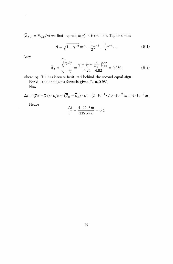
(iJ A,B = VA,s/c) we first express fJ('y) in termsof a Taylor series:

! -2 1 -2 1 -4 /3 = 1 - r = 1 - 2' - s' ... Now

rf

J rdr + .1... + _1_ 15.25

73 A = ri = I 2r 24r3 4.82 = 0.980, IJ - ri 5.25- 4.82

where eq. B.1 has been substituted behind the second equal sign. For 73 8 the analogous formula gives /38 = 0.982. Now

(B.1)

(B.2)

ól = (v B - vA) · L / c = (73 8 - 73 A) · L = (2 · 10-3 · 2.0 · 10-2 m = 4 · 10-5 m.

He nee /:::,.l 4 · 10-

5 m = 0.4.

335 fs · c

79

Appendix C

Listings of Inputfiles

C.l Example of a GPT Inputfile

# --GPT simulation parameters--mm = 1e-3 ; ns = 1e-9 ; ps = 1e-12 fs = 1e-15; mrad=1e-3 microri=1e-6; cm=1e-2; MHz=1e6; #accuracy(7); # --diode parameters-­

gap = 2*mm ; La = 1.5*mm ; diode exit = 0; #gap+ La

# input from Superfish: half acc. cell/coupling cell/acc. cell/coupling cell/acc. cell freq=3011.49515*MHz; fase=-22; # optimum injection phase angle, yields delta W=3.5 MeV

w=freq*2*pi; / ~ phi=fase/deg; ll"f l-(>1P· .. f.fv... map25D_ TM_fix ( "wcs", "z" ,diode_exi t, "final. gdf",

"R", "Z", "Er", "Ez", "Bphi", 1,0 ,phi, w);

# --particles parameters-­ups = 271 Eo = 2e6 G =-q*Eo/(m*c*c) + 1 beta sqrt(1-G--2) Gbeta = G*beta ;

80

# Number of particles # Initial energy [eV] # Corresponding gamma # Corresponding beta # Corresponding gamma*beta

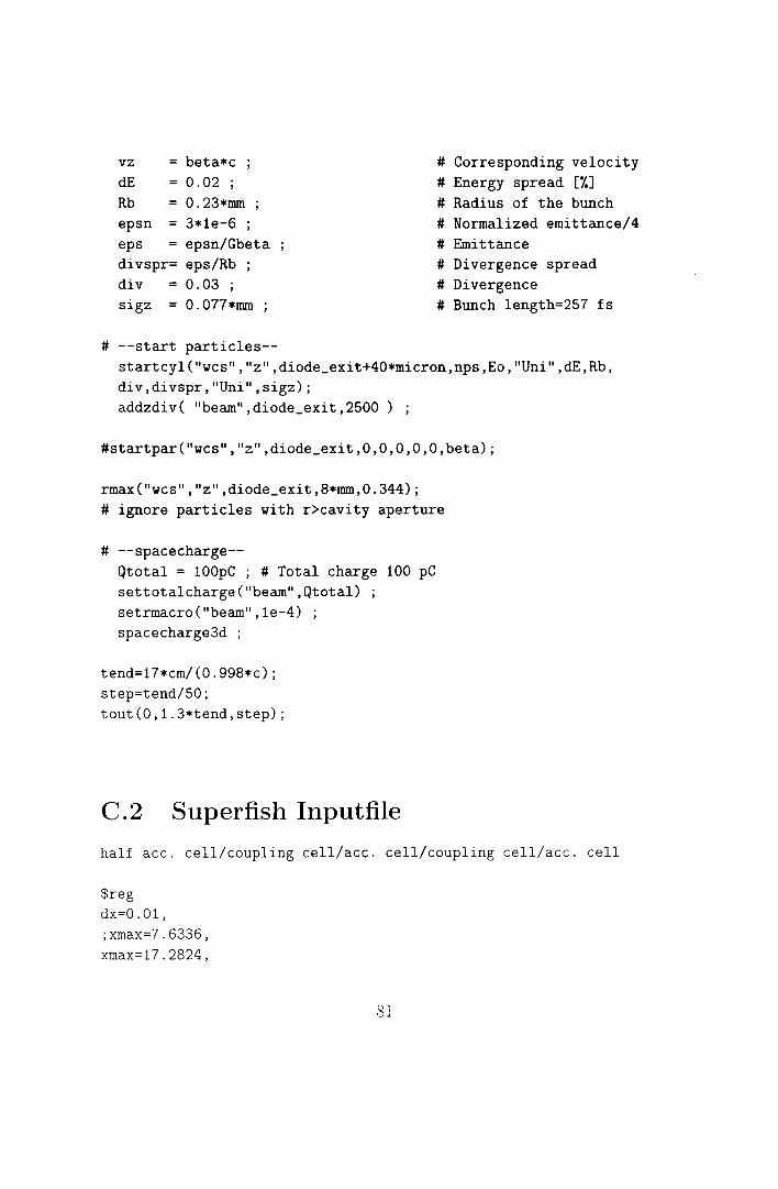
vz beta*c ; # Corresponding velocity dE 0.02 ; # Energy spread [%] Rb = 0.23*nun # Radius of the bunch epsn = 3*1e-6 ; # Norrnalized ernittance/4 eps epsn/Gbeta # Ernittance divspr= eps/Rb ; # Divergence spread div = 0.03 ; # Divergence sigz 0.077*nun # Bunch length=257 fs

# --start particles-­startcyl("wcs","z",diode_exit+40*rnicron,nps,Eo,"Uni",dE,Rb, div,divspr,"Uni",sigz); addzdiv( "bearn",diode_exit,2500) ;

#startpar("wcs","z",diode_exit,O,O,O,O,O,beta);

rrnax("wcs","z",diode_exit,8*nun,0.344); # ignore particles with r>cavity aperture

# --spacecharge--Qtotal = lOOpC ; # Total charge 100 pC settotalcharge("bearn",Qtotal) setrrnacro("bearn",le-4) spacecharge3d ;

tend=17*crn/(0.998*c); step=tend/50; tout(0,1.3*tend,step);

C.2 Superfish Inputfile

half acc. cell/coupling cell/acc. cell/coupling cell/acc. cell

$reg dx=O.Ol, ;xrnax=7.6336, xrnax=17.2824,

81

yreg= 0, 0.7, 1.2942, ymax=3.85, lreg= -1,15,40, lmax=52, freq=3011.35589, xdri=11, ydri=3.85 ezero=20e6$

&po x=O, y=O$ &PO X=O.,Y=3.85 & &PO X=0.6012,Y=3.85& &PO NT=2,X0=0.6012,Y0=2.45, r=l. 4, theta=O& &PO X=2.0012,Y=1.2942& &PO NT=2,X0=1.8012,Y0=1.2942, r=0.2, theta=290.000& &PO X=1.6817,Y=1.0379& &PO NT=2,X0=1.7501,Y0=0.85, r=0.2,theta=180& &PO NT=2,X0=1.6001,Y0=0.85, r=0.05,theta=270& &PO X=2.3512,Y=0.8 & $po nt=2, x0=2.3512, y0=0.95, r=0.15, theta=O$ $po x=2.5012, y=3.5$ $po x=2.7812, y=3.5$ $po x=2.7812, y=0.95$ $po nt=2, x0=2.9312, y0=0.95, r=0.15, theta=270$ $po x=3.6823, y=0.8 $ $po nt=2, x0=3.6823, y0=0.85, r=0.05, theta=O $ $po nt=2, x0=3.5323, y0=0.85, r=0.2, theta=69.968 $ $po x=3.4128, y=1.10626 $ $po nt=2, x0=3.4812, y0=1.2942, r=0.2, theta=180 $ $po x=3.2812, y=2.45 $ $po nt=2, x0=4.6812, y0=2.45, r=1.4, theta=90 $ $po x=5.8836, y=3.85 $ $po nt=2, x0=5.8836, y0=2.45, r=1.4, theta=O $ $po x=7.2836, y=1.2942 $ $po nt=2, x0=7.0836, y0=1.2942, r=0.2, theta=290 $ $po x=6.9641, y=1.0379 $ $po nt=2, x0=7.0325, y0=0.85, r=0.2, theta=180 $ $po nt=2, x0=6.8825, y0=0.85, r=0.05, theta=270 $

82

; 1

;2

;3

;4 ;5

;6 ;7

;8

;9

;10 ;11

;12 ;13 ;14 ;15 ; 16 ;17 ;18 ;19 ;20 ;21 ;22 ;23 ;24 ;25 ;26 ;27 ;28 ;29

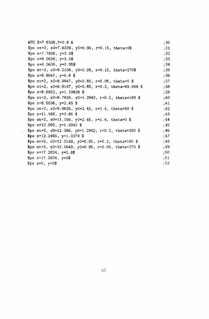
&PO X=7.6336,Y=0.8 & $po nt=2, x0=7.6336, y0=0.95, r=0.15, theta=O$ $po x=7.7836, y=3.5$ $po x=8.0636, y=3.5$ $po x=8.0636, y=0.95$ $po nt=2, x0=8.2136, y0=0.95, r=0.15, theta=270$ $po x=8.9647, y=0.8 $ $po nt=2, x0=8.9647, y0=0.85, r=0.05, theta=O $ $po nt=2, x0=8.8147, y0=0.85, r=0.2, theta=69.968 $ $po x=8.6952, y=1.10626 $ $po nt=2, x0=8.7636, y0=1.2942, r=0.2, theta=180 $ $po x=8.5636, y=2.45 $ $po nt=2, x0=9.9636, y0=2.45, r=1.4, theta=90 $ $po x=11.166, y=3.85 $ $po nt=2, x0=11.166, y0=2.45, r=1.4, theta=O $ $po x=12.566, y=1.2942 $ $po nt=2, x0=12.366, y0=1.2942, r=0.2, theta=290 $ $po x=12.2465, y=1.0379 $ $po nt=2, x0=12.3149, y0=0.85, r=0.2, theta=180 $ $po nt=2, x0=12.1649, y0=0.85, r=0.05, theta=270 $ $po x=17.2824, y=0.8$ $po x=17.2824, y=O$ $po x=O, y=O$

83

;30 ;31 ;32 ;33 ;34 ;35 ;36 ;37 ;38 ;39 ;40 ;41 ;42 ;43 ;44 ;45 ;46 ;47 ;48 ;49 ;50 ;51 ;52