Scientific Report 08-02 Gain calibration of an earthshine ... · albedo baseret på...

Scientific Report 08-02

Gain calibration of an earthshine monitoring instrument

I. Evaluation of the Chae method Hans Gleisner and Peter Thejll

www.dmi.dk/dmi/sr08-02 page 1 of 26 Copenhagen 2008


www.dmi.dk/dmi/sr08-02 page 2 of 26

Colophon Serial title: Scientific Report 08-02 Title: Gain calibration of an earthshine monitoring instrument Subtitle: I. Evaluation of the Chae method Author(s): Hans Gleisner and Peter Thejll Other contributors: Heidi Gross Responsible institution: Danish Meteorological Institute Language: English Keywords: albedo, earthshine, photometry, flat field Url: www.dmi.dk/dmi/sr08-02 Digital ISBN: 978-87-7478-565-1 ISSN: 1399-1949 Version: 2008-09-19 Website: www.dmi.dk Copyright: Danish Meteorological Institute

http://www.dmi.dk/

Scientific Report 08-02 Content: Abstract ................................................................................................................................................4 Resumé.................................................................................................................................................4 1. Introduction......................................................................................................................................5

1.1 Background ................................................................................................................................5 1.2 Scope and limitations of the study .............................................................................................6

2. Fundamentals ...................................................................................................................................7 2.1 Gain calibration and flat-fielding...............................................................................................7 2.2 Gain calibration methods ...........................................................................................................8

2.2.1 Gain calibration using dome flats and twilight sky flats.....................................................8 2.2.2 Gain calibration using multiple, spatially displaced images...............................................8

2.3 Signal-to-noise considerations .................................................................................................10 2.4 Goodness criteria for flat fields................................................................................................10

3. Generation of simulated Earthshine images...................................................................................11 4. Evaluation of Chae’s method.........................................................................................................14

4.1 Light-levels variations vs. flat-field gradients .........................................................................14 4.2 Parameter study........................................................................................................................14

4.2.1 Type of image object – phase of the Moon.......................................................................15 4.2.2 S/N of the input images.....................................................................................................18 4.2.3 Number of displaced images.............................................................................................21 4.2.4 Size of the displacements..................................................................................................22

4.3 Photometric errors....................................................................................................................24 5. Conclusions....................................................................................................................................25 References..........................................................................................................................................26 Previous reports..................................................................................................................................26



Abstract The Earthshine project seeks to develop an automatic telescope-based system for determining terrestrial albedo, for use in climate research, from observations of the earthshine on the Moon. This involves developing accurate methods for obtaining images that are unbiased by instruments arte-facts. This report details the evaluation of a specific flat-fielding method. Different pixels on a CCD, illuminated by the same irradiance, do not respond equally due to differences in pixel sensitivity and imperfections of the optical system. The variation in response, or gain variation, can be deter-mined by taking an image of a totally uniform field – a flat field. This standard method is sufficient to determine the small-scale pixel-to-pixel gain variations but may be less suitable for determination of large-scale gain variations with sufficient precision. Measurement of Earth’s albedo based on Earthshine observations relies on precision photometry involving pixels that are widely separated on the CCD frame and, hence, the standard flat-fielding practices may impose a limitation on the photometric accuracy. In this report we evaluate an alternative method [Chae, 2004a] based on multiple, spatially displaced images of the Moon itself. The evaluation is based on simulated images and, although somewhat limited in scope, shows that this method is able to retrieve the large-scale gain variations from a set of noisy, displaced images. The limitations of the method are discussed and recommendations regarding further investigations of the flat-fielding method are given.

Resumé Jordskinsprojektet handler om at udvikle et automatisk teleskop-baseret system til bestemmelse af jordens albedo, til brug i klimaforskning, udfra observationer af jordskinnet på Månen. Dette kræver udvikling af metoder til optagelse af billeder der ikke har gradient-fejl som følge af instrumentelle bias’er. Denne rapport handler om evaluering af en avanceret metode til såkaldt ’flat-fielding’. Forskellige pixler på en CCD, illumineret af samme irradians, reagerer ikke ens på grund af forskelle i pixel-følsomheden og uhensigtsmæssigheder i det optiske system. Variationen i følsomhed henover CCD’ens flade kan bestemmes ved at tage et billede af en ensartet belyst objekt – som en flad skærm. Denne standardmetode er tilstrækkelige til at fastslå de små pixel-til-pixel variationer, men er mindre egnet til præcis bestemmelse af stor-skala variationer. Måling af Jordens albedo baseret på jordskinsmålinger bygger på præcisions-fotometri ved hjælp af pixels der ligger langt fra hinanden på CCD-rammen og dermed kan den almindelige praksis for ’flatfielding’ reducere den fotometriske nøjagtighed. Vi evaluerer her en alternativ metode [Chae, 2004a] baseret på flere, rumligt forskudte billeder af selve Månen. Evalueringen baseres på simulerede billeder, og selv om undersøgelsen er noget begrænset i omfang, viser den at metoden kan bestemme stor-skala variationer i CCD’ens rummelige gain udfra et sæt støjpåvirkede, forskudte billeder. Begrænsningerne i metoden drøftes og anbefalinger vedrørende yderligere undersøgelser af metoden gives.



1. Introduction 1.1 Background An important factor in governing the radiation balance of the terrestrial climate is the shortwave reflectivity – or albedo – of the Earth. The albedo depends on the surface properties, the amount of clouds, and the abundance of aerosols in the atmosphere. These factors can typically be observed from space. However, space platforms are not easy to calibrate and the introduction of new satel-lites as the old ones reach the end of their service life introduces data discontinuities which high-light problems related to drift in instrument absolute calibrations. In order to help solve this problem an independent source of albedo data is needed and this is possible by using the earthshine that falls on the Moon’s dark side. Photometry from ground based instrumentation observing the Moon over long timescales is necessary, and has been attempted at different times during the 20th century. Lately, a concerted effort to use the latest technology was started in the USA and is now being carried out by the Big Bear Solar Observatory and New Jersey Institute of Technology. In Spain a system is being set up to augment the telescope already installed in California. It is an important goal that a global system of approximately 6 telescopes be set up, in order that coverage of the albedo for all longitudes is provided. Technical issues relating to data stability and observing practise are being developed in a project at the Danish Meteorological Institute and Lund Observa-tory in Sweden, funded by the VINNOVA research agency in Sweden. Some details concerning this project are discussed in other DMI reports [e.g., Thejll, 2004]. Precision photometry using a telescope and a CCD camera requires careful calibration in order to identify and remove instrumental artefacts. One important instrumental effect is the variation in response across the CCD frame due to variations in pixel sensitivity, dust and specks on surfaces, and imperfections of the optical system. The standard method to determine the variation in response is to take an image of a field that is assumed to be totally uniform – the image obtained is referred to as a flat field. While this method is sufficient to determine the small-scale pixel-to-pixel gain variations, it may be less suitable for determination of large-scale gain variations with sufficient precision [Grundahl and Sørensen, 1996; Stubbs and Tonry, 2006]. Measurements of Earth’s albedo based on earthshine observations rely on precision photometry involving pixels that are widely separated on the CCD frame. The most common data reduction strategies rely on spatial averages over many pixels. Hence, it is the large-scale rather than the small-scale variations in instrumental response that may affect the resulting albedos, and the stan-dard flat-fielding practices may impose a limitation on the accuracy achievable. In this DMI techni-cal report we present an evaluation of an alternative method [Chae, 2004a,b] based on multiple, spatially displaced images of the Moon itself. The evaluation is based on simulated images and is somewhat limited in scope. It needs to be followed up by more studies and practical observations.


Scientific Report 08-02 1.2 Scope and limitations of the study The present study address gain variations consisting of a large-scale gradient and a sinusoidal wave pattern across the image. Smaller-scale pixel-to-pixel gain variations are not included in the study. Neither is artefacts produced by the gain calibration procedure itself addressed. Instead we try to evaluate how the signal-to-noise ratio (S/N) of the resulting flat-field frame is affected by:

• the phase of the Moon (i.e., type and spatial extent of the image object) • different S/N of the observed images • the number of observed images used as input to the gain-calibration procedure • choice of displacement strategy

These issues are addressed by a parameter study covering different phases of the Moon (and an ideal Lambert sphere), different S/N of the observed images, a varying number of observed images, and a varying size of the displacement pattern. We also test the proposition that Chae’s method is able to resolve the ambiguity between light level variations (e.g. due to varying exposure times) and flat-field gradients. The most important issues, which may limit the usefulness of the method, but which have not been addressed here are:

• gain variations at all spatial scales • sensitivity to stray light and ghost images • flat-field artefacts caused by telescope pointing errors and the efficiency of cross-correlation

techniques to remedy these effects • flat-field artefacts caused by exposure time variations or atmospheric transparency varia-

tions The results show that the method devised by Chae is able to retrieve the large-scale gain variations from a set of noisy, displaced images, but that the S/N distribution across the flat-field frame is strongly dependent on factors listed above. The limitations of the method are discussed and recom-mendations regarding further investigations of the flat-fielding method are given.


Scientific Report 08-02 2. Fundamentals 2.1 Gain calibration and flat-fielding Even if two pixels on a CCD are illuminated by the same irradiance, they do not necessarily re-spond equally. We refer to this difference in response as a gain variation. One can think of this as due to differences in pixel sensitivity, but it actually includes any image-plane variations due to imperfections of the optical system, dust on surfaces, etc. The procedure of determining the relative gains of the CCD pixels is referred to as gain calibration. Gain calibration is commonly done by taking an image of a field that is supposed to be uniform, e.g. an illuminated screen or the twilight sky. Any variations in such an image are caused by gain variations. We refer to such an image as a flat field. This is also used as a general term to denote a table of the relative gains of the CCD pixels, even when it is not a result of taking an image of a uniform field. The light from the sky entering the telescope has intensity i. Ideally this light produces a signal s during an exposure time, t, so that (1) tis ⋅= However, the signal, d , that we actually measure differs from s because of optical imperfections, dust, and differences in pixel sensitivities across the CCD. We can write

′

(2) bsfd +⋅=′ where f is the gain of the pixel and b is the combined effect of bias and dark current. After subtrac-tion by dark and bias frames (i.e. b), the image recorded by a CCD can be written (3) sfd ⋅= If we divide the observed imperfect image, d, with the flat field, f, we obtain the original signal s. This is the goal of the flat-fielding procedure. A flat field only establishes the relative responses of the pixels. In principle we are free to multiply the entire flat-field frame by an arbitrary constant, but it is common practice to scale the flat field such that it has a maximum close to 1. Unlike the image frames, the flat field takes on floating-point values.


Scientific Report 08-02 2.2 Gain calibration methods

2.2.1 Gain calibration using dome flats and twilight sky flats We have already mentioned that gain calibration can be done by taking an image of an object which is assumed to have a totally uniform brightness. This object can be an illuminated screen at the inside of a telescope dome (“dome flat”) or the evening sky (“sky flat”) [e.g. http://odin.physastro.mnsu.edu/spect_flat.html ]. These methods will not be further discussed here. Suffice it to say that a problem with these methods is the presence of non-uniformities in the source used as flat-field. While pixel-to-pixel gain variations can be obtained with sufficient precision, this may not be the case for large scale variations across the image. For precision photometry involving pixels that are widely separated on the CDD frame, this can be a serious problem.

2.2.2 Gain calibration using multiple, spatially displaced images There are alternative approaches to the traditional dome flats and sky flats. Kuhn, Linz, and Loranz [1991] devised an algorithm (henceforth, the KLL method) to reconstruct the flat pattern f from a set of relatively shifted images of a non-uniform object. The fundamental idea is that if we know that two pixels are exposed to the same irradiance, then the ratio of the pixel responses d is equal to the ratio of the gains f between the two pixels. By taking several exposures of one and the same object, e.g. a dense stellar cluster or the Moon, and displacing the object somewhat between the exposures, we obtain a huge number of such ratios, building up to a linear equation system whose solution gives the gains f of all pixels. The full equation system is exceedingly large and approxima-tions need to be made to obtain a solution. In 2004, Chae [2004a] pointed out a few shortcomings of the KLL method and proposed an alterna-tive method based on the same general principles. In particular, it was claimed that the method devised by Chae solves the problem that differences in the mean signal levels, e.g. due to exposure time variations, may produce a linearly varying artefact pattern in the resulting flat-field frame. Like the KLL method, Chae’s method uses a number of images of the same object differently positioned on the CCD. In practice, one takes several exposures of one and the same object and shifts the image plane spatially such that different pixels are illuminated by the same part of the object. Let the pixels on the CCD be denoted by the row i and column j. Suppose that we take Nf images of one and the same object, where each of these images have been slightly displaced in x (row) and y (column). We denote the displacements by xk and yk, where k is the image number, k=1,…,Nf. Following the notation in Eq. 3, sij is the original signal or ideal image of the object, dij is the actual pixel response, and fij, is the gain of the pixel at row i and column j. The parameter ck accounts for any light level variations between the images, e.g. due to small differences in exposure time. In the unshifted case (4) ijijij

kij nfscd +=

where n is random, zero-mean noise. If the object is shifted by an amount {xk, yk}, then the actually observed image becomes (5) k

ijijj,ikk

ij kknfscd yx += −−


http://odin.physastro.mnsu.edu/spect_flat.html


)

Taking the logarithm of the above expression, and for the moment disregarding the noise, we get (6) ijj,i

kkij loglogloglog

kkfscd yx ++= −−

The basic idea underlying Chae’s method is simply to determine an object image (i.e. original signal) sij, a flat field fij, and a light level ck such that the mean square difference between the logarithms of d and csf is minimized. (7) ( 2

ijkijj,i

kkij

2 loglogloglogkk∑ −−−= −− foca yxχ

In each image, pixels with low data numbers (DN) are masked out and are not allowed to contribute to the resulting equation system. The minimization of Eq. 7 is done iteratively after introducing some simplifying approximations. Chae’s method involves additional complicating details, mainly due to the necessity to deal with boundary effects and the need to reduce the size of the equation system. These details can be found in [Chae, 2004a]. Another consideration is the choice of an efficient dither pattern, i.e. the set of spatial displace-ments. This has consequences for the resulting equation system. In particular, it is important to avoid common multiples in the displacements [Kuhn et al., 1991; Arendt et al., 2000] which may otherwise introduce geometric artefacts in the resulting flat field. In this report we follow the example by Chae [Chae, 2004a] and use displacements generated by taking equally spaced steps along a Reuleaux triangle (see Figure 2). This is further described in Section 3. A precise knowledge of the relative displacements of the images is crucial to this method. In the practical implementation, the displacements are only known approximately. The method has to be combined with some sort of cross-correlation technique to find the true displacements very pre-cisely. Chae [2004a,b] claims to reach sub-pixel accuracy with a Fourier transform cross-correlation technique. In the present study we have avoided this problem by using simulated images for which we know the exact displacements.


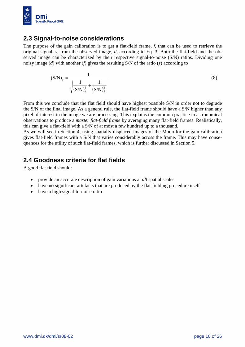
Scientific Report 08-02 2.3 Signal-to-noise considerations The purpose of the gain calibration is to get a flat-field frame, f, that can be used to retrieve the original signal, s, from the observed image, d, according to Eq. 3. Both the flat-field and the ob-served image can be characterized by their respective signal-to-noise (S/N) ratios. Dividing one noisy image (d) with another (f) gives the resulting S/N of the ratio (s) according to

( ) ( )22 S/N1

S/N1

1(S/N)

fd

s

+= (8)

From this we conclude that the flat field should have highest possible S/N in order not to degrade the S/N of the final image. As a general rule, the flat-field frame should have a S/N higher than any pixel of interest in the image we are processing. This explains the common practice in astronomical observations to produce a master flat-field frame by averaging many flat-field frames. Realistically, this can give a flat-field with a S/N of at most a few hundred up to a thousand. As we will see in Section 4, using spatially displaced images of the Moon for the gain calibration gives flat-field frames with a S/N that varies considerably across the frame. This may have conse-quences for the utility of such flat-field frames, which is further discussed in Section 5.

2.4 Goodness criteria for flat fields A good flat field should:

• provide an accurate description of gain variations at all spatial scales • have no significant artefacts that are produced by the flat-fielding procedure itself • have a high signal-to-noise ratio


Scientific Report 08-02 3. Generation of simulated Earthshine images In the present study, we have used simulated images as input to the gain-calibration procedure. We refer to these as the input images. The following types of object have been simulated (see Fig. 1):

• Lambert sphere (i.e. a sphere with a surface that is a perfect lambertian reflector) • Full Moon • Half Moon – western/eastern • Quarter Moon – western/eastern

It is important that the simulated input images have the same general characteristics as actually observed images, particularly regarding the noise. Other features of input images that may influence the ability of a gain calibration method to accurately describe the flat field are the presence, or lack of, stray light and ghost images of instrumental origin. For methods based on displaced images, telescope pointing uncertainties and exposure time variations may also have an influence on the quality of the resulting flat field. In this study, the simulated images were created in the following way:

1. Simulate an image of the Moon or a Lambert sphere using the DMI Earthshine Simulator. The image consists of 1024x1024 square pixels, each covering 2.50 arc-seconds, with pixel values scaled to 75% of 16 bits (i.e. the pixels take on values from 0 to 49152), has zero sky background and no noise. The simulated noise-free images are shown in Figure 1.

2. Take this ideal image and displace it to Nf positions along the Reuleaux triangle. See below for an explanation and definition of the Reuleaux triangle.

3. Add a uniform sky background of 50 counts to the displaced images.

4. Add Gaussian noise with a certain S/N to every pixel in the displaced images. The use of Gaussian rather than Poisson noise means that we can characterize the whole image by a single S/N value.

5. Define a true flat field f0 consisting of a linear gradient from 0.95 at the left edge of the im-age to 1.05 at the right edge, superposed by a sinusoidal with an amplitude 0.02. Multiply this flat field with the displaced, noisy images to produce the final input images. An exam-ple of a set of final, displaced, noisy images is shown in Figure 2.

A Reuleaux triangle can be described as a “fat” triangle. It is constructed by taking an ordinary equilateral triangle and replacing each side by a 60 degree arc connecting two corners while centred on the third, opposite corner. The dither pattern can be described by two parameters: the side L of the triangle (i.e. the side of the corresponding equilateral triangle) and the number of displaced positions Nf along the Reuleaux triangle.



Figure 1. The simulated images used in this study: the Lambert sphere (upper, left panel), the full Moon (upper, right panel), the half Moon (lower, left panel), and the quarter Moon (lower, right panel).



Figure 2. The original ideal image is displaced to Nf (here 15) positions along the Reuleaux triangle (here with size L = 0.35). To each of these Nf displaced images we add a sky background, Gaussian noise, and a gain variation described by a flat field f0.


Scientific Report 08-02 4. Evaluation of Chae’s method 4.1 Light-levels variations vs. flat-field gradients Chae’s method is unable to fully discriminate between a flat-field gradient and systematic light-level variations. Even in the absence of any light-level variations, the factor ck in Eq. 7 is assigned values different from 1.0. In fact, Chae’s method appears to suffer from a gauge freedom of the same type that the other methods based on spatially displaced images suffer from.

4.2 Parameter study For a range of simulated images we have studied the quality of the flat field retrieved by Chae’s method. We have particularly studied the impact of varying:

• type of image object: Lambert sphere, full Moon, half Moon, and quarter Moon • signal-to-noise ratio, S/N, of the input images: from 5 to 1000 • number of displaced images, Nf, used as input to the flat-field processing • size of the displacements: the size, L, of the Reuleaux triangle

Due to the results discussed in Section 4.1 the exposure times were assumed to be constant. Hence, the factor ck in Eq. 6 and 7 was set to a fixed value of 1.0. When interpreting the results it is important to consider that the flat field is only retrieved where at least one input image provides information on the gains. Over parts of the flat-field frame there is simply no information on the gain and this region is masked out during the analysis of the results. Hence, the results discussed in this section only refer to the active part of the flat-field, i.e. those pixels that are not masked. In Section 2.1, it was stated that a flat field only establishes the relative responses of the pixels. A consequence of this is that a retrieved flat-field frame is undetermined to a fixed constant. Before comparing a retrieved flat-field with the true flat-field, we need to normalize the two frames. This is done by giving them the same average over unmasked pixels. Even though the S/N is uniform across the input images, S/N varies across the retrieved flat field. The S/N is highest where many input images provide information on the gains and lowest where few input images provide information. The noise n in the retrieved flat field can be computed as the RMS difference between the retrieved and the true flat fields

( )∑ −=i

ii ffn 2,0N

1

where N is the number of pixels in the region over which we compute the noise, fi is the value of pixel i in the retrieved flat field, and f0,i is the corresponding value of the true flat field. Since the signal always is close to 1, the signal-to-noise ratio S/N is approximately given by 1/n.


Scientific Report 08-02 4.2.1 Type of image object – phase of the Moon Four different image objects were studied: a Lambert sphere, the full Moon, the half Moon, and the quarter Moon. For each of these, flat-fields were retrieved from simulated observations using the following settings for the size of the displacements (L), the number of displaced images (Nf), and the signal-to-noise ratio of the input images (S/N): L = 0.25 Nf = 15 S/N = {5, 10, 20, 50, 100, 500, 1000} For each run, the convergence history up to 50 iterations was recorded. We first note the obvious similarities between the results, as shown by Figs. 3 and 4. There is, however, a clear tendency for a decreasing flat-field S/N when the illuminated fraction of the Moon becomes smaller. This may be understood by a closer look at the results in Figs. 4 and 5.

Figure 3. Convergence histories for the full Lambert sphere (top left panel), the full Moon (top right), the half Moon (lower left), and the quarter Moon (lower right) for different S/N of the input images. The S/N for the retrieved flat field is obtained from the RMS differences between true and retrieved flats computed over the masked region.


Scientific Report 08-02 As described above, gain calibration methods based on displaced images are only able to retrieve a flat field were the input images provide any information on the gain. In the black regions of the flat-field frames in Figure 4, the input images did not contribute any information at all. However, even in regions were a flat field could be retrieved, the amount of information differs significantly, from the central part of the flat fields were all 15 input images contribute, to the periphery where only a few input images contribute. This situation is depicted in Fig. 5.

Figure 4. The retrieved flat fields after 50 iterations for input-image S/N of 100: the Lambert sphere (upper, left panel), the full Moon (upper, right panel), the half Moon (lower left), and the quarter Moon (lower right). The RMS errors between the true flat field and the retrieved flat field only include the masked region.


Scientific Report 08-02 For the full Moon, a large fraction of the active flat-field pixels obtain information from all 15 input images – in Figure 5 there are many white pixels in relation to all active (i.e. grey or white) pixels. For the quarter Moon, the opposite is true – very few pixels obtain information from many input images. If many input images contribute to the information on the gain in a certain pixel, we get a higher S/N in the retrieved flat field. Hence, the full Moon has the highest overall flat-field S/N of all the objects, and as the Moon wanes the S/N of the flat-field decreases.

Figure 5. The more input images that contribute to the information on the gain in a certain pixel, the higher is the S/N of the retrieved flat field. We here see the number of contributing images for the full Moon (right panel), the half Moon (middle panel), and the quarter Moon (right panel). White colour indicates that all 15 images contribute, whereas the darkest gray indicates that only 1 image contribute. In black regions, no input images at all contribute. Hence these areas are masked out, and are not a part of the flat-fielding procedure, as seen in Figure 4.


Scientific Report 08-02 4.2.2 S/N of the input images For the full Moon, flat-fields were retrieved from simulated observations using the following settings for the size of the displacements (L), the number of displaced images (Nf), and the signal-to-noise ratio of the input images (S/N): L = 0.25 Nf = 15 S/N = {5, 10, 20, 50, 100, 500, 1000} For each run, the convergence history up to 50 iterations was recorded. The convergence histories and the retrieved flat fields for a range of signal-to-noise ratios of the input images have been discussed in Section 1.4.1. In Figure 6, it is shown how the overall S/N of the retrieved flat-field scale with the S/N of the input images. As might be expected the relation is very close to linear – the higher the input image S/N, the higher the S/N of the retrieved flat field.

Figure 6. Relation between the S/N of the input images and the overall S/N of the retrieved flat field.


Scientific Report 08-02 In Fig. 7 we show the retrieved and true flat field along one row in the flat-field frame, while the differences between these two are shown in Fig. 8. Both the linear trend and the sinusoidal wave patterns are accurately described by the retrieved flat field. The noise in the retrieval seems to originate solely in the noise of the input images.

Figure 7: The retrieved flat along a CCD row for different signal-to-noise ratios of the input images, for the case of the full Moon. Both the linear trend and the sinusoidal wave patterns are accurately described by the retrieved flat field.


Scientific Report 08-02 The differences between the retrieved and true flat fields (Figure 8) clearly show that the noise in the retrieval is smallest in the centre and increases towards the periphery. This is most likely due to the effects described in Section 1.4.1 – the number of input images contributing to the flat-field retrieval is largest in the middle and decreases further out.

Figure 8: The differences between the retrieved and true flat fields along a CCD row for different signal-to-noise ratios of the input images, for the case of the full Moon.


Scientific Report 08-02 4.2.3 Number of displaced images For the full Moon, flat-fields were retrieved from simulated observations using the following settings for the size of the displacements (L), the number of displaced images (Nf), and the signal-to-noise ratio of the input images (S/N): L = 0.25 Nf = {5, 10, 15, 20, 40} S/N = {20, 1000} Increasing the number of displaced images, Nf, increases the overall S/N of the retrieved flat field. The increase is roughly proportional to the square root of Nf fN∝S/N which is the same relation as for arithmetic averaging of noisy images. The reason for not being closer to an exact proportionality when computing an overall S/N for the flat-field frame is that a fraction of the pixels are based on information from less than Nf input images.

Figure 9: Increasing the number of displaced images, Nf, increases the S/N of the retrieved flat field. The increase is roughly proportional to the square root of Nf.


Scientific Report 08-02 4.2.4 Size of the displacements For the full Moon, flat-fields were retrieved from simulated observations using the following settings for the size of the displacements (L), the number of displaced images (Nf), and the signal-to-noise ratio of the input images (S/N): L = {0.10, 0.15, 0.20, 0.25, 0.35, 0.50, 0.70} Nf = 15 S/N = {20, 1000} Increasing the size of the displacements, L, decreases the overall S/N of the retrieved flat-field frame. The reason is that with larger L, a larger fraction of the active flat-field pixels are based on information from less than Nf input images. This effect is depicted in Figure 11, where the number of input images contributing to the flat-field pixel value is indicated by shaded grey – white corre-sponding to 15 and black to 0. This effect is similar to the effect of changing the phase of the Moon, described in Section 4.2.1. We also note that smaller displacements, L, require more iterations to fully converge.

Figure 10: Increasing the size, L, of the displacements leads to a decrease in the flat-field S/N. Smaller displacements L require more iterations to fully converge.



Figure 11: Increasing the size, L, of the displacements leads to a decrease the flat-field S/N. With larger L, a larger fraction of the active flat-field pixels are based on information from less than Nf input images. Here the number of input images contributing to the flat-field pixel value is indicated by a shaded grey – white corresponds to 15 and black to 0. From top left to bottom right, the displacements L are 0.10, 0.20, 0.25, 0.35, 0.50, and 0.70.


Scientific Report 08-02 4.3 Photometric errors In earthshine observations, aiming at the measurement of terrestrial albedo, we are primarily inter-ested in the data number ratio between two pixels, or pixel groups, that are widely separated on the CCD frame. Any errors in the estimation of large-scale flat-field patterns have a detrimental effect on such ratios. A ratio between two pixels located at opposite sides of a CCD would be in error by a factor of about 10% if we assumed that the flat field was truly uniform while in reality it had a gradient going from 0.95 at one side of the frame to 1.05 at the other side. The nature of errors due to an incorrect estimation of the flat field are different from the random errors in that they are systematic – they can not be reduced by averaging over many pixels or many images. Errors in the estimates of the flat field are directly related to biases in the derived albedos. We now repeat the study described in Section 4.2.3 (“Number of displaced images”), but instead of quantifying the goodness of the derived flat field by the RMS error relative to the true flat field, we quantify the goodness by estimating the photometric errors made in using the derived flat field. Define two patches in the flat fields, both consisting of 100 pixels and separated by 30 arc-seconds. Then compute separate averages over the two patches in each flat-field frame. We refer to these averages as 1f and 2f . For the true flat-field frame we refer to the corresponding averages as true

1f , and true

2f . The relative error in the ratio of these pixel values is

true1

true2

true1

true2

1

2

ff

ff

ff−

=Δ

This quantity is directly proportional to the relative error in the derived terrestrial albedo. Precision photometry in earthshine observations requires errors well below 1%, preferably in the order of 0.1%. This seems to be achievable in principle with the method studied here.

Figure 12: Photometric errors due to errors in the estimation of large-scale flat field patterns, for input images with a S/N of 20 (left) and 1000 (right) and using a varying number of images as input to the gain calibration procedure. The requirement on the photometric precision is in the order of 0.1% in earthshine observations.


Scientific Report 08-02 5. Conclusions In this study, the ability of the gain calibration method devised by Chae [Chae, 2004a,b] has been tested using simulated images of the Moon. We conclude that with Chae’s method applied to images of the Moon, we can efficiently retrieve a gain variation pattern consisting of a large-scale gradient combined with a sinusoidal wave patter. The S/N ratio of the retrieved flat field depends on the S/N of the input images, the number of displaced images used in the retrieval, the size and pattern of displacements, and the phase of the Moon. The two last factors also determine the spatial structure of the retrieved flat field – parts of the flat-field frame are left undetermined and can not be used. These results are not difficult to understand in general terms. Between the S/N of the retrieved flat field and the S/N of the input images there is a simple linear relationship. At the same time, the S/N of the flat field increases roughly proportional to the square root of the number, Nf, of input images. This is the same relation as for averaging noisy images. The detailed relationship between the flat field S/N and the phase of the Moon, or the flat-field S/N and the pattern of displacements, can be understood by considering the number of input images actually contributing to the pixels in differ-ent parts of the flat-field frame. For the full Moon a large fraction of the active flat-field pixels are covered by all Nf input images, while for the quarter Moon the average number of input images contribution to the gain calibration is much smaller than Nf. A drawback of the method is the fact that the flat-field S/N varies considerably across the frame, and that for a realistic dithering strategy large parts of the flat-field frame are left undetermined. The scope of this study was limited. Small-scale pixel-to-pixel variations were not included in the study. More importantly, we did not study any artefacts produced by the gain calibration method itself. For a thorough assessment of the practical utility of the gain calibration method, this is required. We particularly need to investigate:

• flat-field artefacts caused by telescope pointing errors and the efficiency of cross-correlation techniques to remedy these effects

• flat-field artefacts produced by exposure time variations or atmospheric transparency varia-tions

• the sensitivity of the gain-calibration method to stray light and ghost images Another issue, specific to an Earthshine telescope equipped with an occulting device is:

• how to gain calibrate an optical system that includes an occulting disk Nevertheless, the study results show that this method of gain calibration has a potential to overcome some of the limitations of more traditional gain calibration methods – e.g. dome flats – in that it appears to be able to account for gradients and other large-scale structures in the CCD pixel gains. This is also seen in that the photometric errors due to errors in the determination of large-scale flat-field patterns are well below 1% even for very unfavourable conditions, and for more favourable conditions a photometric precision in the order of 0.1% seems to be achievable.




References Arendt, R.G., Fixsen, D.J., and Moseley, S.H., Dithering strategies for efficient self-calibration of

imaging arrays, Astrophys. J., 536, 500-512, 2000.

Chae, J.-C., Flat-fielding of solar Halfa observations using relatively shifted images, Solar Physics, 221, 1-14, 2004a.

Chae, J.-C., Flat-fielding of solar magnetograph observations using relatively shifted images, Solar Physics, 221, 15-21, 2004b.

Denker, C, Johannesson, A., Marquette, W., Goode, P.R., Wang, H., and Zirin, H., Synoptic Halfa full-disk observations of the Sun from Big Bear Solar Observatory, Solar Physics, 184, 87-102, 1999.

Fixsen, D.J., Moseley, S.H., and Arendt, R.G., Calibrating array detectors, Astrophys. J. Suppl., 128, 651-658, 2000.

Grundahl, F., and Sørensen, A.N., Detection of scattered light in telescopes, Astron. Astrophys. Suppl., 116, 367-371, 1996.

Kuhn, J.R., Lin, H., and Loranz, D., Gain calibrating nonuniform image-array data using only the image data, PASP, 103, 1097-1108, 1991.

Stubbs, C.W., and Tonry, J.L., Toward 1% photometry: end-to-end calibration of astronomical telescopes and detectors, Astrophys. J., 646, 1436-1444, 2006.

Thejll, P.A. An automatic earthshine telescope. A pilot project , DMI Technical report No. 04-18, 2004.

Toussaint, R.M., and Harvey, J.W., Improved convergence for CCD gain calibration using simulta-neous-overrelaxation techniques, Astron. J, 126, 1112-1118, 2003.

Previous reports Previous reports from the Danish Meteorological Institute can be found on: http://www.dmi.dk/dmi/dmi-publikationer.htm

http://www.dmi.dk/dmi/dmi-publikationer.htm

Scientific Report 08-02 Gain calibration of an earthshine ... · albedo baseret på...

Documents

Transcript of Scientific Report 08-02 Gain calibration of an earthshine ... · albedo baseret på...