1

Road Design and ConstructionIn

Sensitive Watersheds

Dr. Peter SchiessForest Engineering

University of WashingtonSeattle, WA 98115

and

Carol A. WhitakerHydrologist

Crown - ZellerbachLongview, WA 98632

for

Forest Conservation branchForest Resources Division

Forestry Department

Food and Agriculture Organizationof the United Nations

Rome, Italy1986

2

Table of Contents

CHAPTER 1 _______________________________________________________________ 15

DEFINITION AND SCOPE OF PROTECTIVE MEASURES FOR ROADS __________ 15

1.1 General Introduction ____________________________________________________________________ 15

1.2 Interaction of Roads and Environment______________________________________________________ 15

1.3. Erosion Processes. ______________________________________________________________________ 17

1.4 Assessment of Erosion Potential ___________________________________________________________ 181.4.1 Surface Erosion ______________________________________________________________________ 181.4.2. Mass Soil Movement _________________________________________________________________ 25

CHAPTER 2 _______________________________________________________________ 30

ROAD PLANNING AND RECONNAISSANCE__________________________________ 30

2.1 Route Planning _________________________________________________________________________ 302.1.1 Design Criteria ______________________________________________________________________ 312.1.2 Design Elements _____________________________________________________________________ 35

2.1.2.2 Road width______________________________________________________________________ 372.1.2.3. Turnouts _______________________________________________________________________ 392.1.2.4. Turn-arounds ___________________________________________________________________ 422.1.2.5. Curve Widening_________________________________________________________________ 422.1.2.6 Clearance_______________________________________________________________________ 432.1.2.7. Speed and Sight Distance _________________________________________________________ 432.1.2.8. Horizontal and Vertical Alignment __________________________________________________ 432.1.2.9. Travel Time ____________________________________________________________________ 45

2.2 Economic Evaluation and Justification______________________________________________________ 482.2.1 Economic Analysis Methods ____________________________________________________________ 482.2.2 Analysis of Alternative Routes __________________________________________________________ 49

2.3 Route Reconnaissance and Location ________________________________________________________ 542.3.1 Road Reconnaissance _________________________________________________________________ 542.3.2 Faults______________________________________________________________________________ 612.3.3 Indicators of Slope Stability ____________________________________________________________ 64

CHAPTER 3 _______________________________________________________________ 69

ROAD DESIGN_____________________________________________________________ 69

3.1 Horizontal and Vertical Alignment _________________________________________________________ 69

3

3.1.1 Horizontal Alignment Considerations _____________________________________________________ 693.1.2 Curve Widening _____________________________________________________________________ 723.1.3 Vertical Alignment ___________________________________________________________________ 84

3.2 Road Prism ____________________________________________________________________________ 883.2.1 Road Prism Stability __________________________________________________________________ 883.2.2 Side Cast - Full Bench Road Prism _______________________________________________________ 923.2.3 Slope design ________________________________________________________________________ 963.2.4 Road Prism Selection ________________________________________________________________ 103

3.3 Road Surfacing ________________________________________________________________________ 107

CHAPTER 4 ______________________________________________________________ 118

DRAINAGE DESIGN_______________________________________________________ 118

4.1 General Considerations _________________________________________________________________ 118

4.2 Estimating runoff ______________________________________________________________________ 121

4.3 Channel Crossings______________________________________________________________________ 1264.3.1 Location of Channel Crossings _________________________________________________________ 1264.3.2 Fords _____________________________________________________________________________ 1274.3.3 Culverts ___________________________________________________________________________ 1294.3.4 Debris Control Structures _____________________________________________________________ 1474.3.5 Bridges ___________________________________________________________________________ 150

4.4 Road Surface Drainage__________________________________________________________________ 1514.4.1 Surface Sloping _____________________________________________________________________ 1514.4.2 Surface Cross Drains_________________________________________________________________ 1534.4.3 Ditches and Berms___________________________________________________________________ 1594.4.4 Ditch Relief Culverts_________________________________________________________________ 166

CHAPTER 5 ______________________________________________________________ 174

SURFACE AND SLOPE PROTECTIVE MEASURES ___________________________ 174

5.1 Introduction___________________________________________________________________________ 174

5.2 Surface Protection Measures _____________________________________________________________ 1745.2.1 Site Analysis _______________________________________________________________________ 1765.2.2 Site Preparation _____________________________________________________________________ 1765.2.3 Seeding and Planting_________________________________________________________________ 1775.2.4 Application Methods _________________________________________________________________ 1785.2.5 Wattling and filter strips ______________________________________________________________ 1815.2.6 Brush Layering _____________________________________________________________________ 1835.2.7. Mechanical Treatment _______________________________________________________________ 185

5.3 Mass Movement Protection ______________________________________________________________ 185

4

CHAPTER 6 ______________________________________________________________ 193

ROAD CONSTRUCTION TECHNIQUES _____________________________________ 193

6.1 Road Construction Techniques ___________________________________________________________ 1936.1.1 Construction Staking _________________________________________________________________ 1936.1.2. Clearing and Grubbing of the Road Construction Area ______________________________________ 196

6.2 General Equipment Considerations _______________________________________________________ 1976.2.1 Bulldozer in Road Construction ________________________________________________________ 1976.2.2 Hydraulic Excavator in Road Construction________________________________________________ 202

6.3 Subgrade Construction__________________________________________________________________ 2046.3.1 Subgrade Excavation with Bulldozer ____________________________________________________ 2046.3.2 Fill Construction ____________________________________________________________________ 2086.3.3 Compaction ________________________________________________________________________ 2106.3.5 Filter Windrow Construction___________________________________________________________ 213

5

List of Figures

Figure 1 Sediment production in relation to road density (Amimoto, 1978).______________________________ 16

Figure 2. Infinite slope analysis for planar failures _________________________________________________ 25

Figure 3. Relationship between frictional resistance (F) and driving force (E) promoting downslope movement.(Burroughs, et al., 1976). _____________________________________________________________________ 27

Figure 4. Sixty cm of soil with 15 cm of ground water will slide when the slope gradient exceeds 58 percent.(Burroughs, et al., 1976) ______________________________________________________________________ 27

Figure 5. (a) Subsurface rainwater flows in the direction of the slope when geologic strata dip toward the slope. (b)Subsurface rainwater percolates downward and out of the root zone when geologic strata dip in that direction (Rice,1977). ____________________________________________________________________________________ 28

Figure 6. Road structural terms. _______________________________________________________________ 35

Figure 7. Turnout spacing in relation to traffic volume and travel delay time. ____________________________ 39

Figure 8. Typical turnout dimensions ___________________________________________________________ 41

Figure 9. Relationship between curve radius and truck speed when speed is not controlled by grade.__________ 44

Figure 10. Relationship between grade and truck speed on gravel roads.________________________________ 45

Figure 11. Stepped backslope (no scale)._________________________________________________________ 52

Figure 12. Tag line location and centerline location of proposed road. Sideslopes are typically less than 40 to 50percent. ___________________________________________________________________________________ 55

Figure 13. Tag line location and centerline location of proposed road. Sideslopes are typically 50% or steeper. _ 55

Figure 14. Selection of the road alignment in the field by "stretching the tag line"; This "stretched", or "adjusted"tagline is surveyed and represents the final horizontal location of the road. _________________________________ 56

Figure 15. Position [1] shows tag line ribbon at approximately eye-level. The feet of the road locator are "ongrade". Position [2] shows the ribbon on-location over the centerline or tangent as selected in the field afterstretching. The ribbon has been moved horizontally, thereby allowing an estimate of required cut or fill at centerline._________________________________________________________________________________________ 56

Figure 16. Example of the effect of shortened centerline through a draw or around a sharp ridge. This situationdevelops when running the tag line into the draw or around a sharp ridge without allowing for proper curve layoutand design location.__________________________________________________________________________ 57

Figure 17. Curve layout by deflection method, a useful approach during the original road location phase.______ 58

Figure 18. By sighting across draw at 0 percent grade, the desired curve is laid out without increasing the grade. 59

Figure 19. Cut and fill apportioning through a switchback to maintain a given grade. ______________________ 61

6

Figure 20. Suspected fault zones are indicated by the alignment of saddles in ridges and by the direction of streamchannels. Geologic map is found in upper left corner. Major faults are shown as heavy dark lines on geologic maps(Burroughs,et al.,1976) _______________________________________________________________________ 62

Figure 21. Stereogram of a possible fault zone. The location of the fault is indicated by the dashed line through thelow saddle between the large, older slump at A and the newer slope failure at B (Burroughs, et al.,1976). ______ 63

Figure 22. Approximate boundary between serpentine (metamorphic rock) material and the Umpqua formation isshown by the dashed line. The determination is based primarily on the basis of vegetation density. Timber onportions of the Umpqua formation have been harvested which accounts for a reduction in vegetation density,particularly in the northwest corner of the photo. (Burroughs, et al., 1976) ______________________________ 64

Figure 23. "Hummocky" topography with springs, curved or tilted trees, and localized slumps characterize landundergoing active soil creep.___________________________________________________________________ 65

Figure 24. Empirical headwall rating system.used for shallow, rapid landslides on the Mapleton Ranger District,U.S. Forest Service, Region 6, Oregon. __________________________________________________________ 67

Figure 25. Non-geometric and conventional p-line traverses__________________________________________ 69

Figure 26. Design adjustments. ________________________________________________________________ 70

Figure 27. Full bench design. __________________________________________________________________ 71

Figure 28. Self-balanced design ________________________________________________________________ 71

Figure 29. Basic vehicle geometry in off-tracking __________________________________________________ 72

Figure 30. Example of truck-trailer dimensions. ___________________________________________________ 74

Figure 31. Step 1. Graphical solution of curve widening ____________________________________________ 75

Figure 32. Steps 2 and 3; Graphical solution for curve widening. ______________________________________ 76

Figure 33. Graphical solution for off-tracking of a stinger-type log truck ________________________________ 77

Figure 34. Curve widening and taper lengths._____________________________________________________ 79

Figure 35. Curve widening guide for a two or three axle truck as a function of radius and deflection angle. Thetruck dimensions are as shown._________________________________________________________________ 80

Figure 36. Curve widening guide for a truck-trailer combination as a function of radius and deflection angle. Thedimensions are as shown. _____________________________________________________________________ 81

Figure 37. Curve widening guide for a log-truck as a function of radius and deflection angle. The dimensions are asshown. ____________________________________________________________________________________ 82

Figure 38. Curve widening guide for a tractor/trailer as a function of radius and deflection angle. The tractor-trailerdimensions are as shown. _____________________________________________________________________ 83

Figure 39. Typical vertical curves( VPI = Vertical Point of Intersection). _______________________________ 84

Figure 40. Vertical curve elements (VPC = Vertical Point of Curvature; VPT = Vertical Point of Tangency ).___ 86

7

Figure 41. Log truck geometry and dimensions for vertical curve analysis _______________________________ 87

Figure 42. Translational or wedge failure brought about by saturated zone in fill. Ditch overflow or unprotectedsurfaces are often responsible. _________________________________________________________________ 90

Figure 43. Fill failure caused by backward erosion at the toe of the fill due to excessive seepage and an unprotectedtoe. ______________________________________________________________________________________ 91

Figure 44. Elements of road prism geometry ______________________________________________________ 93

Figure 45. Required excavation volumes for side cast and full bench construction as function of side slope.Assumed subgrade width 6.6 m and bulking factor K = 1.35 (rock).____________________________________ 94

Figure 46. Erodible area per kilometer of road for side cast construction as a function of side slope angle and cutslope angle. The values shown are calculated for a 6.6 m wide subgrade. The fill angle equals 37o. __________ 95

Figure 47. Erodible area per kilometer of road for full bench/end haul construction as a function of side slope angleand cut slope angle. The values shown are calculated for a 6.6 m wide subgrade.. _________________________ 96

Figure 48. Maximum cut slope ratio for coarse grained soils with plastic fines (low water conditions). Each curveindicates the maximum height or the steepest slope that can be used for the given soil type. (After USFS,1973) _ 100

Figure 49. Maximum cut slope angle for coarse grained soils with plastic fines (high water conditions). Each curveindicates the maximum cut height or the steepest slopes that can be used for the given soil type. (After USFS,1973)________________________________________________________________________________________ 100

Figure 50. Maximum cut slope angle for fine grained soils with slowly permeable layer at bottom of cut. Each curveindicates the maximum vertical cut height or the steepest slope that can be used for the given soil type. (After USFS1973)____________________________________________________________________________________ 101

Figure 51. Maximum cut slope angle for fine grained soils with slowly permeable layer at great depth (> 3 timesheight of cut) below cut. (After USFS, 1973). ___________________________________________________ 102

Figure 52. Interaction of subgrade dimension, roadwidth, ballast depth, ditch width and fill widening ________ 104

Figure 53. Fill widening added to standard subgrade width where fill height at centerline or shoulder exceeds acritical height. Especially important if sidecast construction instead of layer construction is used.____________ 105

Figure 54. Template and general road alignment projected into the hill favoring light to moderate cuts at centerlinein order to minimize fill slope length. Fill slopes are more succeptible to erosion and sloughing than cut slopes. 106

Figure 55. Illustration of the very considerable reduction in excavation made possible on a steep slope by the use ofcribbing. Crib proportions shown are suitable for log construction; if crib was built of concrete or steel, shorterspreaders could be used in upper 3 m as indicated by the dashed line (Kraebel, 1936)._____________________ 107

Figure 56. Ballast thickness curves for single wheel loads (from Steward, et al., 1977). Conversion factors: 1 inch =2.5 cm ; 1kg/cm2 = 14.22 psi._________________________________________________________________ 114

Figure 57. Ballast thickness curves for dual wheel loads (from Steward, et al., 1977). Conversion factors: 1 inch =2.5 cm ; 1kg/cm2 = 14.22 psi._________________________________________________________________ 115

8

Figure 58. Ballast thickness curves for tandem wheel loads (form Steward et al 1977). Conversion factors: 1inch =2.5 cm; 1kg/cm2 = 14.22 psi. _________________________________________________________________ 116

Figure 59. Slope shape and its impact on slope hydrology. Slope shape determines whether water is dispersed orconcentrated. (US Forest Service,1979)_________________________________________________________ 119

Figure 60. Culvert and road locations have modified drainage patterns of ephemeral streams 2 and 3. Locations Aand B become potential failure sites. Stream 3 is forced to accept more water below B due to inadequate drainage atA._______________________________________________________________________________________ 120

Figure 61. Determining high water levels for measurement of stream channel dimensions. _________________ 124

Figure 62. Ford construction stabilized by gabions placed on the downstream end. (Megahan, 1977) _________ 127

Figure 63. Profile view of stream crossing with a ford. A dip in the adverse grade provideschanneling preventingdebris accumulation from diverting the stream on to and along the road surface. The profile of the ford along withvehicle dimensions must be considered to insure proper clearance and vehicle passage. (After Kuonen, 1983)__ 128

Figure 64. Hardened fill stream crossings provide an attractive alternative for streams prone to torrents or debrisavalanches (Amimoto, 1978). _________________________________________________________________ 129

Figure 65. Possible culvert alignments to minimize channel scouring. (USDA, Forest Service, 1971) ________ 131

Figure 66. Proper culvert grades. (Highway Task Force, 1971) ______________________________________ 132

Figure 67. Definition sketch of variables used in flow calculations. ___________________________________ 133

Figure 68. Hydraulics of culverts (Highway Task Force, 1971) ______________________________________ 134

Figure 70. Nomograph for concrete pipes, inlet control (U.S. Dept. of Commerce, 1963) __________________ 141

Figure 71. Nomograph for corrugated metal pipe (CMP), inlet control. (U.S. Dept. of Commerce,1963). _____ 142

Figure 72. Nomograph for corrugated metal arch pipe (CMP), inlet control. (U.S. Dept. of Commerce, 1963). 143

Figure 73. Nomograph for box - culvert, inlet control. (U.S. Dept. of Commerce, 1963). _________________ 144

Figure 74. Nomograph for corrugated metal pipe (CMP), outlet control. (U.S. Dept. of Commerce, 1963).____ 145

Figure 75. Proper pipe foundation and bedding (1 ft. = 30 cm). (USDA, Forest Service, 1971) _____________ 146

Figure 76. Debris control structure--cribbing made of timber.________________________________________ 147

Figure 77. Debris control structure--trash rack made of steel rail (I-beam) placed over inlet.________________ 148

Figure 78. Inlet and outlet protection of culvert with rip-rap. Rocks used should typically weigh 20 kg or more andapproximately 50 percent of the rocks should be larger than 0.1 m3 in volume. Rocks can also be replaced withcemented sand layer (1 part cement, 4 parts sand)._________________________________________________ 149

Figure 79. Road cross section grading patterns used to control surface drainage. _________________________ 151

9

Figure 80. Design of outsloped dips for forest roads. A to C, slope about 10 to 15 cm to assure lateral flow; B, nomaterial accumulated at this point - may require surfacing to prevent cutting; D, provide rock rip-rap to preventerosion; E, berm to confine outflow to 0.5 m wide spillway. (Megahan, 1977)___________________________ 153

Figure 81. Design of insloped dips for forest roads. A to C, slope about 10 to 15 cm to assure lateral flow; B, nomaterial accumulated at this point - may require surfacing to prevent cutting; D, provide rock rip-rap to preventerosion; E, berm to prevent overflow; F, culvert to carry water beneath road; G, widen for ditch and pipe inlet(Megahan, 1977). __________________________________________________________________________ 154

Figure 82. Installation of an open-top culvert. Culverts should be slanted at 30 degrees downslope to help preventplugging. Structure can be made of corrugated steel, lumber or other, similar material. (Darrach, et al., 1982) _ 155

Figure 83. Cross ditch construction for forest roads with limited or no traffic. Specifications are generalized andmay be adjusted for gradient and other conditions. A, bank tie-in point cut 15 to 30 cm into roadbed; B, cross drainberm height 30 to 60 cm above road bed; C, drain outlet 20 to 40 cm into road; D, angle drain 30 to 40 degreesdowngrade with road centerline; E, height up to 60 cm, F, depth to 45 cm; G, 90 to 120 cm. (Megahan, 1977) _ 155

Figure 84. Spacing standard for open-top culverts on forest road surfaces, Japanese Islands. (Minematsu andMinamikata,1983)__________________________________________________________________________ 157

Figure 85. Guide for locating cross drains. Several locations require cross drains independent of spacing guides. Aand J, divert water from ridge; A, B, and C, cross drain above and below junction; C and D, locate drains below loglanding areas; D and H, drains located with regular spacing; E, drain above incurve to prevent bank cutting and keeproad surface water from entering draw; F, ford or culvert in draw; G, drain below inside curve to prevent water fromrunning down road; I, drain below seeps and springs. (Megahan, 1977) ________________________________ 158

Figure 86. Ditch interception near stream to divert ditch water onto stable areas instead of into the stream. (U. S.Environmental Protection Agency,1975) ________________________________________________________ 161

Figure 87. Minimum ditch dimensions. _________________________________________________________ 162

Figure 88. Nomograph for solution of Manning's equation (U.S. Dept. of Commerce, 1965)________________ 164

Figure 89. Minimum berm dimensions. _________________________________________________________ 166

Figure 90. Ditch relief culvert installation showing the use of headwall, downspout and a splash barrier/energydissipator at the outlet. Minimum culvert grade is 3 to 5 percent. Exit velocities should be checked. (U. S.Environmental Protection Agency, 1975) ________________________________________________________ 167

Figure 91. Ditch relief culvert in close proximity to live stream showing rock dike to diffuse ditch water andsediment before it reaches the stream. (U. S. Environmental Protection Agency, 1975) ____________________ 168

Figure 92. Energy dissipators. (Darrach, et al., 1981)______________________________________________ 168

Figure 93. Size of stone that will resist displacement by water for various velocities and ditch side slopes._____ 169

Figure 94. Selection criteria for slope stabilization methods. ________________________________________ 175

Figure 95. Selection criteria for surface cover establishment methods in relation to erosion risk._____________ 180

Figure 96. Preparation and installation procedure for contour wattling, using live willow stakes (after Kraebel,1936). ___________________________________________________________________________________ 183

10

Figure 97. Brush layer installation for slope stabilization using rooted plants for cut slope and green branches for fillslope stabilization.__________________________________________________________________________ 184

Figure 98. Types of retaining walls.____________________________________________________________ 187

Figure 99. Forces acting on a retaining wall. _____________________________________________________ 188

Figure 100. Example of a standard crib wall design. (Wash. State Dept. of Highways) ___________________ 190

Figure 101. Low gabion breast walls showing sequence of excavation, assembly, and filling. (From White andFranks,1978) ______________________________________________________________________________ 191

Figure 102. Road cross section showing possible construction information. _____________________________ 194

Figure 103. The effect of improperly starting the cut as marked by the slope stake. Starting the cut too high resultsin excess excavation and side cast. Starting the cut too low leaves an oversteepened cut bank. ______________ 195

Figure 104. Construction grade check. Engineer stands on center of construction grade and sights to RP tag.Measured distance and slope allow for determination of additional cut. ________________________________ 195

Figure 105. Clearing limits in relation to road bed widths. Significant quantities of organic materials are removedbetween B and E. Stumps are removed between B and D. Stumps may be left between D and E. Organic debris andremoved stumps are placed in windrows at F to serve as filter strips (see Section 6.3.1). ___________________ 196

Figure 106. Pioneer road location at bottom of proposed fill provides a bench for holding fill material of completedroad. ____________________________________________________________________________________ 197

Figure 107. Maximum production rates for different bulldozers equipped with straight blade in _____________ 199

Figure 108. Adjustment factors for bulldozer production rates in relation to grade. (Caterpillar PerformanceHandbook, 1984) __________________________________________________________________________ 201

Figure 109. Fill slope length reduction by means of catch-wall at toe of fill. (See also Figure 55) ___________ 203

Figure 110. Three basic road prism construction methods___________________________________________ 205

Figure 111. Road construction with a bulldozer; The machine starts at the top and in successive passes excavatesdown to the required grade. Excavated material is side cast and may form part of the roadway. _____________ 206

Figure 112. Sliver fills created on steep side slopes where ground slope and fill slope angles differ by less than 7oand fill slope height greater than 6.0 meters are inherently unstable. ___________________________________ 207

Figure 113. Trench-excavation to minimize sidehill loss of excavation material. Debris and material falls into trenchin front of the dozer blade. Felled trees and stumps are left to act as temporary retaining walls until removed duringfinal excavation. ___________________________________________________________________________ 208

Figure 114. Fills are constructed by layering and compacting each layer. Lift height should not exceed 50 cm.Compaction should be done with proper compaction equipment and not a bulldozer (from OSU Ext. Service 1983).________________________________________________________________________________________ 209

Figure 115. Fills that are part of the roadway should not be constructed by end dumping. (from OSU Ext. Service,1983). ___________________________________________________________________________________ 209

11

Figure 116. Excavation cost comparison for three different embankment construction techniques (1 cu.yd. = 0.9m3). (after Haber and Koch,1983) _____________________________________________________________ 211

Figure 117. First pass with excavator, clearing logs and stumps from construction site. Working platform or pioneerroad just outside of planned road surface width.___________________________________________________ 212

Figure 118. Second pass with excavator, removing or stripping overburden or unsuitable material and placing itbelow pioneer road._________________________________________________________________________ 213

Figure 119. Third pass, finishing subgrade and embankment fill over pioneer road. Road side ditch is finished at thesame time. ________________________________________________________________________________ 213

Figure 120. Typical filter windrow dimensions built of slash and placed on the fill slope immediately above the toe.The windrow should be compressed and the bottom part embedded 15 cm in the fill slope. (after Cook and King,1983)____________________________________________________________________________________ 215

12

List of Tables

Table 1 Unified Soil Classification System (adapted from U.S. Department of Interior, Bureau of Reclamation, EarthManual , Denver)____________________________________________________________________________17

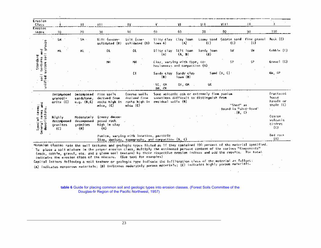
table 2 Guide for placing common soil and geologic types into erosion classes. (Forest Soils Committee of theDouglas-fir Region of the Pacific Northwest, 1957)__________________________________________________18

table 3 Traffic service levels definitions used to identify design parameters (from U.S. Forest Service,Transportation Eng.Handbook)_________________________________________________________________________________27

table 4 Example of a roads objective documentation form (from U.S. Forest Service, Transportation Eng.Handbook)_________________________________________________________________________________29

table 5 Traveled way widths for single-lane roads___________________________________________________ 37

table 6 Lane widths for double-lane roads ________________________________________________________ 38

table 7 Recommended turnout spacing--all traffic service levels _______________________________________ 39

table 8 Turnout widths and lengths______________________________________________________________ 42

table 9 Curve widening criteria_________________________________________________________________ 42

table 10 Relationship between round trip travel time per kilometer and surface type as influenced by vertical andhorizontal alignment; adverse grade in direction of haul (U.S. Forest service, 1965). ______________________ 46

table 11 Relationship between round trip travel time per kilometer and surface type as influenced by vertical andhorizontal alignment; favorable grade in direction of haul (U.S. Forest service, 1965)._____________________ 47

table 12 Comparison of single-lane versus double-lane costs at three different use levels. ___________________ 50

table 13 Comparison of annual road costs per kilometer -- 10,000 vehicles per year. _______________________ 51

table 14 Comparison of annual road costs per kilometer for 20,000 and 40,000 ___________________________ 51

table 15 Cost summary comparison (5 vehicles per hour--1/2 logging trucks, 1/2 other traffic); assumes 8-hourhauling day, 140 days/year use, 20 year road life, 23.8 m3 (6.0 M bd. ft.) loads for logging trucks, cost of operatinglogging trucks including driver's wage--$0.25/min, cost of operating other vehicles--$0.04/minute, 5,535 m3 (1 1/2MM bd. ft.) timber harvested. (Gardner, 1978) ____________________________________________________ 53

table 16 Deflection angles for various chord lengths and curve radii. ___________________________________ 58

table 18 Values of friction angles and unit weights for various soils. (from Burroughs, et. al., 1976) __________ 89

table 19 Maximum cut slope ratio for coarse grained soils. (USFS, 1973) _______________________________ 99

table 20 Maximum cut slope ratio for bedrock excavation (USFS, 1973) ________________________________ 99

table 21 Minimum fill slope ratio for compacted fills. (US Forest Service, 1973) ________________________ 103

13

table 22 Required subgrade width (exclusive fo fill widening) as a function of road width, ballast depth and ditchwidth. Roadwidth = 3.0 m, ditch = 0.9 m (1:1 and 2:1 slopes), shoulder-slopes 2:1. ______________________ 104

table 23 Calculated sediment yield per kilometer of road for various road types and use levels (Reid, 1981; Reid andDunne, 1984)*_____________________________________________________________________________ 108

table 24 Engineering characteristics of soil groups for road construction (Pearce, 1960).___________________ 110

table 25 Required depth of ballast for three design vehicles. Road designed to withstand large traffic volumes ( >1,000 axle loads) with less than 5 cm of rutting.___________________________________________________ 113

table 26 Flood recurrence interval (years) in relation to design life and probability of failure.* (Megahan, 1977) 121

table 27 Values of relative imperviousness for use in rational formula. (American Iron and Steel Institute, 1971) 123

table 28 Manning's n for natural stream channels (surface width at flood stage) __________________________ 124

table 29 Relationship of peak flow with different return periods. (Nagy, et al, 1980)______________________ 125

table 30 Values for coefficient of roughness (n) for culverts. (Highway Task Force,1971) _________________ 134

table 31 Effect of in-sloping on sediment yield of a graveled, heavily used road segment with a 10 % down grade fordifferent cross slopes*_______________________________________________________________________ 152

table 32 Cross drain spacing required to prevent rill or gully erosion deeper than 2.5 cm on unsurfaced logging roadsbuilt in the upper topographic position 1/ of north-facing slopes2/ having gradient of 80 % 3/ (Packer, 1967).__ 156

table 33 Maximum permissible velocities in erodible channels, based on uniform flow in straight, continuously wet,aged channels. For sinuous channels, multiply allowable velocity by 0.95 for slightly sinuous, 0.9 for moderatelysinuous, and 0.8 for highly sinuous channels. (U. S. Environmental Protection Agency, 1975) ______________ 159

table 35 Ditch velocities for various n and grades. Triangular ditch with side slope ratio of 1:1 and 2:1, flowing 0.30meters deep; hydraulic radius R=0.12. __________________________________________________________ 163

table 37 Erosion control and vegetation establishment effectiveness of various mulches on highways in eastern andwestern Washington. Soils: silty, sandy and gravelly loams, glacial till consisting of sand, gravel and compacted siltsand clays (all are subsoil materials without topsoil addition). Slope lengths: approximate maximum of 50 m (165 ft).Application rates: Cereal straw - 5,500 kg/ha (2 t/ac); Straw plus asphalt - 5,500 kg/ha (2 t/ac) and 0.757 l/kg (200gal/t), respectively; Wood cellulose fiber - 1,345 kg/ha (1,200 lbs/ac); Sod - bentgrass strips 46 cm (18 in) by 1.8 m(6 ft) pegged down every third row. ____________________________________________________________ 178

table 38 Windrow protective strip widths required below the shoulders1 of 5 year old2 forest roads built on soilsderived from basalt3, having 9 m cross-drain spacing4, zero initial obstruction distance5, and 100 percent fill slopecover density6. ____________________________________________________________________________ 182

table 39 Road construction equipment characteristics (from OSU Extension Service, 1983)________________ 198

table 40 Job condition correction factors for estimating bulldozer earth moving production rates. Values are fortrack-type tractor equipped straight (S) blade. ( Caterpillar Handbook, 1984) ___________________________ 200

table 41 Approximate economical haul limit for a 185 hp bulldozer in relation to grade. (Production rates achievedare expressed in percent of production on a 10 percent favorable grade with 30 m haul. (Pearce, 1978) _______ 202

14

table 42 Average production rates for a medium sized bulldozer (12-16 tonnes) constructing a 6 to 7 m widesubgrade. _________________________________________________________________________________ 202

table 43 Production rates for hydraulic excavators in relation to side slopes, constructing a 6 to 7 m wide subgrade.________________________________________________________________________________________ 203

table 44 Fill slope erosion volume for windrowed and nonwindrowed slopes during a 3 year period followingconstruction (Cook and King,1983).____________________________________________________________ 213

15

CHAPTER 1

DEFINITION AND SCOPE OF PROTECTIVE MEASURES FOR ROADS

1.1 General Introduction

This handbook was written as a guide to reducing environmental impacts of forest roads in mountainwatersheds and is intended to be used by professional land managers involved in decisions regarding uplandconservation, watershed management, and watershed rehabilitation. Its purpose is to (1) identify potentialthreats to water quality from the construction and maintenance of roads, and (2) recommend procedures,practices, or methods suitable for preventing, minimizing, or correcting erosion problems. It discusses properplanning, reconnaissance, road standard development, erosion control, slope stabilization, drainage design,and maintenance techniques as well as cost analysis procedures that can be applied in the design,construction, and maintenance of forest roads. Specific questions relating to road design procedures, generallayout and construction methods can be found elsewhere, and it is left to the reader to locate sources for thattype of information.

The types of roads considered here would generally be built to withstand low to moderate traffic levelsfor purposes of providing access for residents, timber harvesting, reforestation, rangeland management, andother multiple use activities where access to upland areas is required. Availability of some basic heavyequipment, such as bulldozers and graders, is assumed. Whenever possible, emphasis will be given to labor-rather than machinery-intensive methods. However, livestock or human labor may often be substitutedwherever machines are mentioned and may in fact be preferable to the use of machines by reducingenvironmental impacts during operations. This is especially true in the case of road maintenance. Productionrates in most cases will be much slower and should be considered when developing cost estimates.

Much of the information cited here reflects years of research and experience gained from varioussources. As such, the material presented must be evaluated in light of local geographic, economic, andresource needs; it cannot and should not be a substitute for regional knowledge, experience, and judgment.

1.2 Interaction of Roads and Environment

Forest roads are a necessary part of forest management. Road networks provide access to the forestfor harvests, for fire protection and administration, and for non-timber uses such as grazing, mining, andwildlife habitat. New road construction is required to enter previously uninhabited areas or underutilizedlands, and will continue to provide access in order to properly manage those lands.

Construction and use of forest roads result in changes to the landscapes they cross. Of all the types ofsilvicultural activities, improperly constructed and inadequately maintained "logging roads" are the principalhuman-caused source of erosion and sediment. (US Environmental Protection Agency, 1975) Road failuresand surface erosion can exert a tremendous impact on natural resources and can cause serious economiclosses because of blocked streams, degraded water quality, destroyed bridges and road rights-of-way, ruinedspawning sites, lowered soil productivity, and property damage.

Erosion is related, among other things, to:

1. Physical factors. These would include soil type, geology, and climate (rainfall).

16

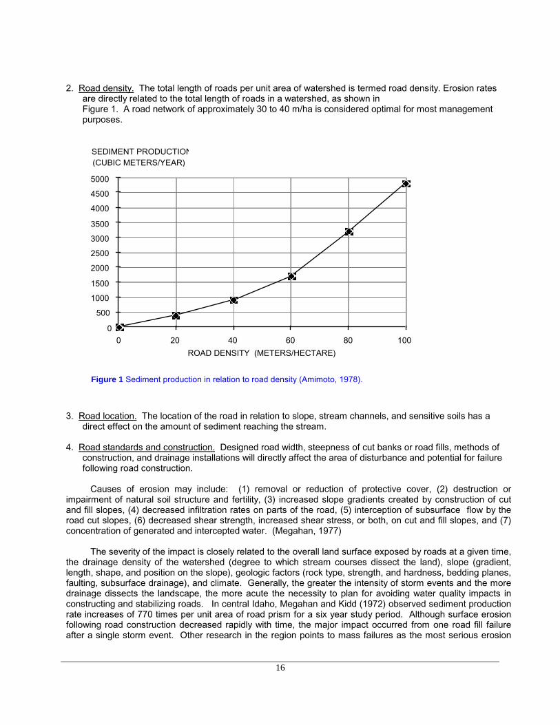
2. Road density. The total length of roads per unit area of watershed is termed road density. Erosion ratesare directly related to the total length of roads in a watershed, as shown inFigure 1. A road network of approximately 30 to 40 m/ha is considered optimal for most managementpurposes.

0

500

1000

1500

2000

2500

3000

3500

4000

4500

5000

0 20 40 60 80 100ROAD DENSITY (METERS/HECTARE)

SEDIMENT PRODUCTION(CUBIC METERS/YEAR)

Figure 1 Sediment production in relation to road density (Amimoto, 1978).

3. Road location. The location of the road in relation to slope, stream channels, and sensitive soils has adirect effect on the amount of sediment reaching the stream.

4. Road standards and construction. Designed road width, steepness of cut banks or road fills, methods of

construction, and drainage installations will directly affect the area of disturbance and potential for failurefollowing road construction.

Causes of erosion may include: (1) removal or reduction of protective cover, (2) destruction orimpairment of natural soil structure and fertility, (3) increased slope gradients created by construction of cutand fill slopes, (4) decreased infiltration rates on parts of the road, (5) interception of subsurface flow by theroad cut slopes, (6) decreased shear strength, increased shear stress, or both, on cut and fill slopes, and (7)concentration of generated and intercepted water. (Megahan, 1977)

The severity of the impact is closely related to the overall land surface exposed by roads at a given time,the drainage density of the watershed (degree to which stream courses dissect the land), slope (gradient,length, shape, and position on the slope), geologic factors (rock type, strength, and hardness, bedding planes,faulting, subsurface drainage), and climate. Generally, the greater the intensity of storm events and the moredrainage dissects the landscape, the more acute the necessity to plan for avoiding water quality impacts inconstructing and stabilizing roads. In central Idaho, Megahan and Kidd (1972) observed sediment productionrate increases of 770 times per unit area of road prism for a six year study period. Although surface erosionfollowing road construction decreased rapidly with time, the major impact occurred from one road fill failureafter a single storm event. Other research in the region points to mass failures as the most serious erosion

17

process contributing to reduced water quality on forest lands. (Swanson and Dyrness, 1975; Fredriksen,1970; Dyrness, 1967; Megahan, 1967)

It is well documented that water quality impacts caused by roads can best be dealt with by prevention orby minimizing their effects, rather than attempting to control damage after it has occurred (Brown, 1973;Megahan, 1977). This can best be done by minimizing the total mileage of roads through proper planning,properly locating roads in relation to topography and soils, minimizing exposed constructed road surfaces byproper road standard selection and alignment, and using proper road construction and culvert installationtechniques.

Additionally, these same researchers have found that the majority of sediment generated on roadsoccurs within the first year following construction. This would emphasize the need for concurrent erosioncontrol measures during and immediately following construction. Merely seeding bare soil surfaces may notbe sufficient to curb soil erosion.

1.3. Erosion Processes.

Recognition of the type of erosion occurring on an area and knowledge of factors controlling erosion areimportant in avoiding problem areas and in designing control structures. Erosion can be broadly categorizedas surface erosion and mass erosion. Mass erosion includes all erosion where particles tend to move enmasse primarily under the influence of gravity. It includes various types of landslides and debris torrents.Surface erosion is defined as movement of individual soil particles by forces other than gravity alone such asoverland flow or runoff, raindrop impact, and wind. Dry creep or dry ravel, the movement of individual particlesresulting from wetting and drying, freezing and thawing, or mechanical disturbance, is considered a surfaceerosion process.

Surface erosion is a function of three factors: (1) the energy available from erosion forces(raindrop splash, wind, overland flow, etc.), (2) the inherent erosion hazard of the site (soil physical andmineralogical characteristics, slope gradient, etc.), and (3) the amount and type of cover available to protectthe soil surface (vegetation, litter, mulch, etc.). Mass erosion is controlled by the balance between stabilizingfactors (root strength, cohesion) and destabilizing factors (slope gradient, seepage forces, groundwater)operating on a hillslope. Another way of stating this relationship is the relative magnitude of shear strengthversus shear stress. When shear stress is less than or equal to shear strength, the slope will remain stable;when stress exceeds strength, the slope will fail.

Factors that might be considered when assessing the impact of road construction and subsequentdevelopment of a site might include:

Soil and Geologysoil - physical and chemical characteristicsgeologic conditions (stratigraphy, mineralogy, etc.)groundwater occurrence and movementslope stabilityseismic characteristics

Climate and Precipitationstart and end of rainy seasonintensity and duration of stormsoccurrence of summer stormsseasonal temperaturefrost-free periodwind erosionsnow melt runoff

18

rainfall runoff before and after development

Topographyslope angleslope aspectslope lengthdensity and capacity of drainagewayssuitability of sites for sediment basins

Vegetative Covertype and location of native plantsfire hazardease in establishing vegetative coveradequacy of existing plants in reducing erosion

Manner of Developmentpercent grade and layout of roadsdensity of roadsdistribution of open spacestructures affecting erodible areasnumber of culverts, stream crossingssize of areas, duration and time of year when groundis left bare

1.4 Assessment of Erosion Potential

1.4.1 Surface Erosion

Soil properties important in the evaluation of a site for its resistance to erosion include particle size,permeability, water retention characteristics, compressibility, shear strength, void ratio or porosity, shrink-swellpotential, liquid limit and plasticity index. Soil developmental characteristics such as horizonation, depth tobedrock or parent material, and depth to seasonal water table are also helpful. Other factors which influenceerodibility include vegetation characteristics (foliage density, height above soil surface, rooting characteristics)and litter cover. Raindrop energy may be partially dissipated by overstory or understory vegetation, therebyreducing the amount of energy transmitted directly to the soil surface. The litter layer contributes the most inprotecting the soil from erosion by absorbing the net energy that finally reaches the surface after filteringthrough vegetation canopies. Any surface runoff that may occur on a natural soil surface will generally takeplace below the litter layer, however, the flow velocity is very slow because of the tortuosity of the path that thewater must take to pass through the litter. Particle detachment, therefore, is unlikely where good litter cover ispresent.

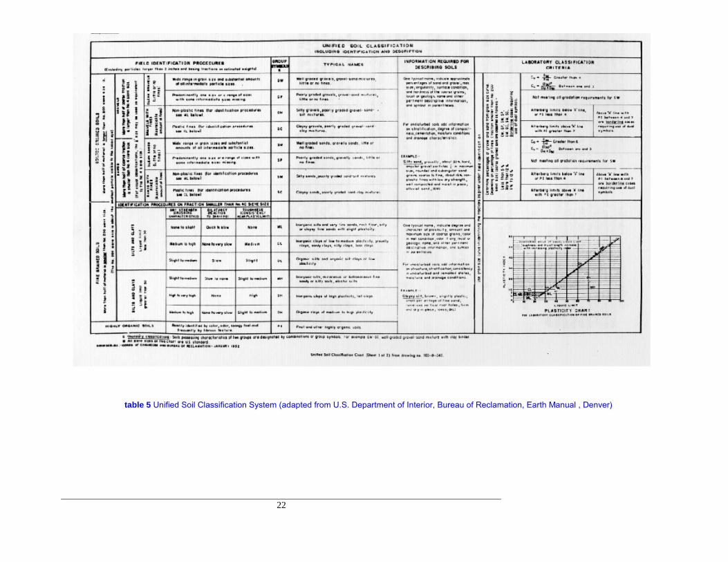
In order to discuss soil characteristics in a uniform and accurate manner, several classification systemshave been developed which provide guidance in identifying a particular soil's desirability or value for variousengineering uses. The Unified Engineering Soil Classification system was developed as a method of groupingsoils for military construction and is shown in Table 1. Other classification systems include the United StatesDepartment of Agriculture Soil Textural Classification system and the American Association of State Highwaysand Transportation Officials (AASHTO) system.

A guide for evaluating soil erosion potential in the field can be made by visual inspection of the soil andby such techniques as shaking, patting, and kneading. Subsurface samples can be extracted with the use ofhand augers or shovels. Classification of soils into erodibility groups based on the Unified System is presented

19

in Table 2. A discussion of erodibility in relation to cross-drain spacing requirements is presented in Chapter3.4.3.

Several methods are available in order to evaluate the potential for soil loss from surface erosion, andtwo different approaches have been utilized in estimating surface soil loss. The first of these is empirical innature using predictive equations developed from analysis of "real" data. The second consists of the use ofprocess models--models developed through analysis of cause and effect relationships. The empiricalprocedure most commonly used is the Universal Soil Loss Equation (USLE) which was originally developedfor use on Midwestern United States agricultural soils and has since been modified for use in forestenvironments. The Modified Soil Loss Equation (MSLE) uses a vegetation management factor (VM) toreplace the cropping factor (C) and the erosion control practice factor (P) used in the USLE (U. S.Environmental Protection Agency, 1980). The MSLE is:

A = R K L S VMwhere:

A = estimated average soil loss per unit area in tons/acre for the time period selected for R(usually one year)

R = rainfall factor, usually expressed in units of rainfall erosivity index (EI) and evaluated froman iso-erodent map

K = soil erodibility factor, usually expressed in tons/acre/EI units for a specific soil in cultivatedcontinuous fallow, tilled up and down the slope

L = slope length factor expressed as the ratio of soil loss from the field slope length to that froma 72.6 foot (22.1 meter) length on the same soil, gradient, cover, and management

S = slope gradient factor expressed as the ratio of soil loss from a given field gradient to thatfrom a 9 percent slope with the same soil, cover, and management

VM = vegetation management factor expressed as the ratio of soil loss from land managed under specific conditions to that from the fallow condition on which the factor K isevaluated.

Numerical values for each of the factors are based on research data and differ dramatically from oneregion to another, from one locality to another, and even from one field to another. However, approximatevalues for potential soil loss from a site may be calculated with the understanding that strict adherence to theassumptions made in selecting values for individual factors is required if a reasonable answer is to beobtained. Even so, errors in the range of an order of magnitude of the true erosion rate are not uncommon. Aprocedural guide in using the MSLE is presented in Chapter IV, An Approach to Water Resources Evaluationof Non-Point Silvicultural Sources, US Forest Service, 1980.

20

22

table 5 Unified Soil Classification System (adapted from U.S. Department of Interior, Bureau of Reclamation, Earth Manual , Denver)

tab

23

le 6 Guide for placing common soil and geologic types into erosion classes. (Forest Soils Committee of theDouglas-fir Region of the Pacific Northwest, 1957)

25

1.4.2. Mass Soil Movement

Accurate models and data needed to predict mass soil movement over broad areas are currentlylacking. A widely used technique involves the relatively simple planar infinite slope analysis described by Sidle(1985). This method is particularly useful when the thickness of soil is small in comparison to the length ofslope and where the failure plane parallels the soil surface. The infinite slope model is illustrated in Figure 2 .

Figure 2. Infinite slope analysis for planar failures

The forces acting on the soil mass "a b c d" in Figure 2 include the vegetative weight per unit area, WT,and the weight of soil WS which give rise to the tangential and normal shear stresses acting on line a-b. Theheight of the water table is MZ. The vertical height of water above the slide plane, designated M, is a fractionof the soil thickness, Z, above the plane.

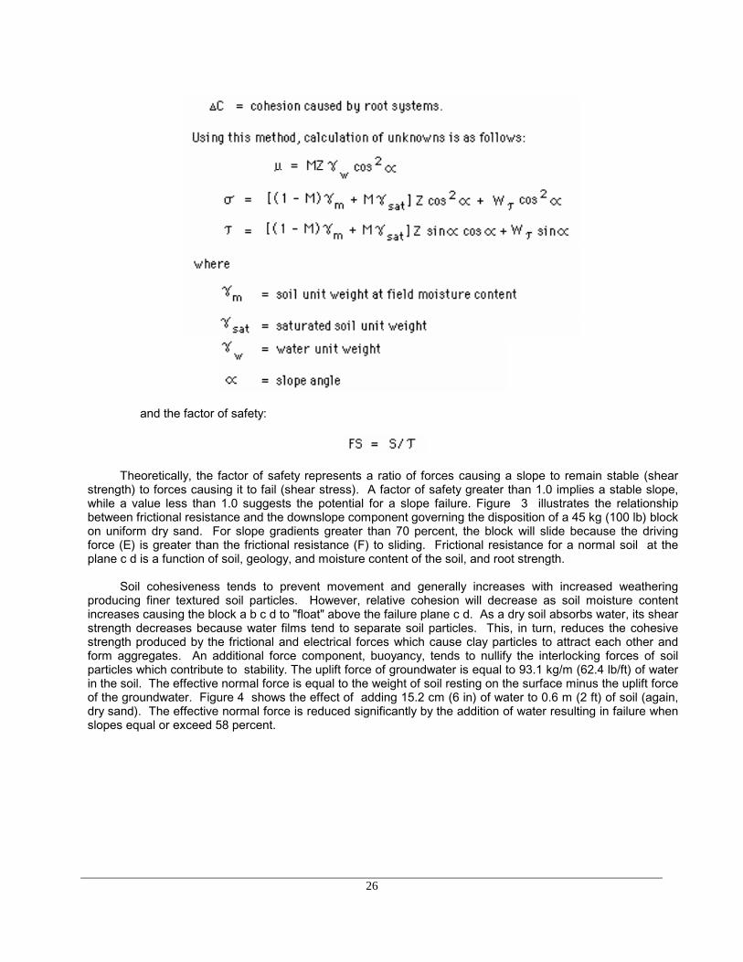
The resistance to failure or shear strength S along line a-b is:

26

and the factor of safety:

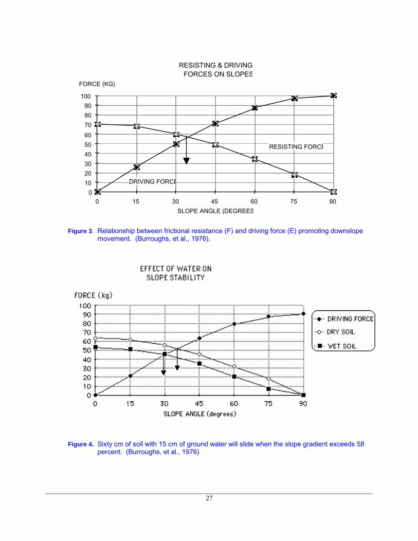
Theoretically, the factor of safety represents a ratio of forces causing a slope to remain stable (shearstrength) to forces causing it to fail (shear stress). A factor of safety greater than 1.0 implies a stable slope,while a value less than 1.0 suggests the potential for a slope failure. Figure 3 illustrates the relationshipbetween frictional resistance and the downslope component governing the disposition of a 45 kg (100 lb) blockon uniform dry sand. For slope gradients greater than 70 percent, the block will slide because the drivingforce (E) is greater than the frictional resistance (F) to sliding. Frictional resistance for a normal soil at theplane c d is a function of soil, geology, and moisture content of the soil, and root strength.

Soil cohesiveness tends to prevent movement and generally increases with increased weatheringproducing finer textured soil particles. However, relative cohesion will decrease as soil moisture contentincreases causing the block a b c d to "float" above the failure plane c d. As a dry soil absorbs water, its shearstrength decreases because water films tend to separate soil particles. This, in turn, reduces the cohesivestrength produced by the frictional and electrical forces which cause clay particles to attract each other andform aggregates. An additional force component, buoyancy, tends to nullify the interlocking forces of soilparticles which contribute to stability. The uplift force of groundwater is equal to 93.1 kg/m (62.4 lb/ft) of waterin the soil. The effective normal force is equal to the weight of soil resting on the surface minus the uplift forceof the groundwater. Figure 4 shows the effect of adding 15.2 cm (6 in) of water to 0.6 m (2 ft) of soil (again,dry sand). The effective normal force is reduced significantly by the addition of water resulting in failure whenslopes equal or exceed 58 percent.

27

0102030405060708090

100

0 15 30 45 60 75 90

RESISTING & DRIVINGFORCES ON SLOPES

SLOPE ANGLE (DEGREES

FORCE (KG)

RESISTING FORCE

DRIVING FORCE

Figure 3. Relationship between frictional resistance (F) and driving force (E) promoting downslopemovement. (Burroughs, et al., 1976).

Figure 4. Sixty cm of soil with 15 cm of ground water will slide when the slope gradient exceeds 58percent. (Burroughs, et al., 1976)

28

The problems and limitations in applying this or similar models are many. Estimation of these factors isextremely difficult given the high degree of anisotrophy and heterogeneity of soil properties. Detailed analysisof factors leading to failure of natural slopes, especially piezometric information, is lacking. As difficult as theprediction of the factor of safety is, predicting the course or type of deformation a failure will take is far moredifficult. The contribution of plant root systems in reinforcing the soil matrix is often significant but difficult toquantify.

The orientation of the underlying geologic strata plays an important part in overall stability. Whenbedding planes are oriented in the direction of the slope (Figure 5a), potential zones of weakness and failuresurfaces are ready-made. Additionally, the beds will tend to concentrate subsurface water and return it to thesurface. Any excavation on such slopes may also remove support and create excessive road maintenanceproblems by rock and soil sliding on to the road. Conversely, geologic strata which are more or less normal tothe surface slope (Figure 5b) resist sliding since weakness in the bedding planes do not contribute to thedownslope component nor do they concentrate percolating rainwater near the surface.

Figure 5. (a) Subsurface rainwater flows in the direction of the slope when geologic strata diptoward the slope. (b) Subsurface rainwater percolates downward and out of the root zonewhen geologic strata dip in that direction (Rice, 1977).

Other factors influencing slope stability include seepage forces exerted by groundwater as it movesdownslope through the soil and support provided by live tree roots in contributing to soil strength. Although notfully understood, the presence of root strength is most important where soils are shallow and where winterstorms can cause groundwater levels to rise sharply. Roots tend to anchor shallow soils on steep slopes tofractures in the underlying rock. Reports from US Forest Service researchers in Alaska indicate that thenumber of landslides from cut-over areas increases within 3 to 5 years after logging--about the time when rootdecay becomes nearly complete. (Bishop and Stevens, 1964) Researchers in Japan and the U. S. have

29

found that root systems of different species have differing decay rates. Rice (1977) postulates that harvestscheduling according to relative contribution of a particular specie's root system to slope stability might provideadditional support to slopes at or near threshold strength values.

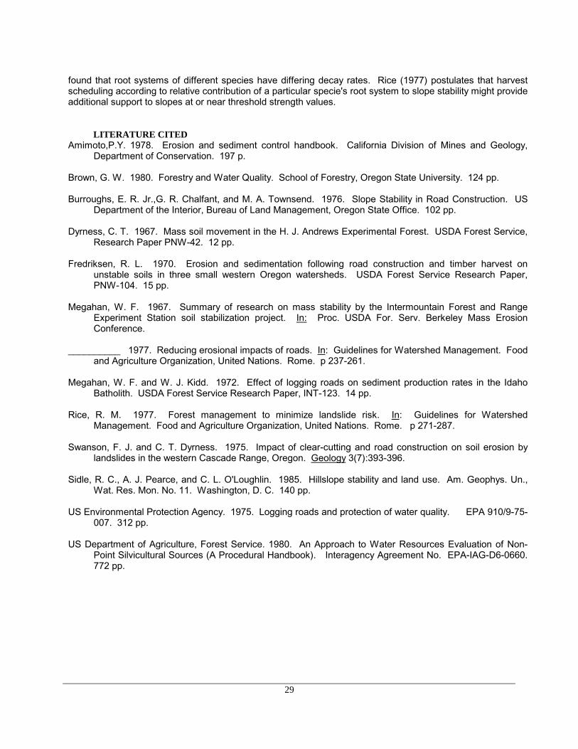
LITERATURE CITEDAmimoto,P.Y. 1978. Erosion and sediment control handbook. California Division of Mines and Geology,

Department of Conservation. 197 p.

Brown, G. W. 1980. Forestry and Water Quality. School of Forestry, Oregon State University. 124 pp.

Burroughs, E. R. Jr.,G. R. Chalfant, and M. A. Townsend. 1976. Slope Stability in Road Construction. USDepartment of the Interior, Bureau of Land Management, Oregon State Office. 102 pp.

Dyrness, C. T. 1967. Mass soil movement in the H. J. Andrews Experimental Forest. USDA Forest Service,Research Paper PNW-42. 12 pp.

Fredriksen, R. L. 1970. Erosion and sedimentation following road construction and timber harvest onunstable soils in three small western Oregon watersheds. USDA Forest Service Research Paper,PNW-104. 15 pp.

Megahan, W. F. 1967. Summary of research on mass stability by the Intermountain Forest and RangeExperiment Station soil stabilization project. In: Proc. USDA For. Serv. Berkeley Mass ErosionConference.

__________ 1977. Reducing erosional impacts of roads. In: Guidelines for Watershed Management. Foodand Agriculture Organization, United Nations. Rome. p 237-261.

Megahan, W. F. and W. J. Kidd. 1972. Effect of logging roads on sediment production rates in the IdahoBatholith. USDA Forest Service Research Paper, INT-123. 14 pp.

Rice, R. M. 1977. Forest management to minimize landslide risk. In: Guidelines for WatershedManagement. Food and Agriculture Organization, United Nations. Rome. p 271-287.

Swanson, F. J. and C. T. Dyrness. 1975. Impact of clear-cutting and road construction on soil erosion bylandslides in the western Cascade Range, Oregon. Geology 3(7):393-396.

Sidle, R. C., A. J. Pearce, and C. L. O'Loughlin. 1985. Hillslope stability and land use. Am. Geophys. Un.,Wat. Res. Mon. No. 11. Washington, D. C. 140 pp.

US Environmental Protection Agency. 1975. Logging roads and protection of water quality. EPA 910/9-75-007. 312 pp.

US Department of Agriculture, Forest Service. 1980. An Approach to Water Resources Evaluation of Non-Point Silvicultural Sources (A Procedural Handbook). Interagency Agreement No. EPA-IAG-D6-0660.772 pp.

30

CHAPTER 2

ROAD PLANNING AND RECONNAISSANCE

2.1 Route Planning

Planning with respect to road construction takes into account present and future uses of thetransportation system to assure maximum service with a minimum of financial and environmental cost. Themain objective of this initial phase of road development is to establish specific goals and prescriptions for roadnetwork development along with the more general location needs. These goals must result from acoordinated effort between the road engineer and the land manager, forester, geologist, soil scientist,hydrologist, biologist and others who would have knowledge or recommendations regarding alternatives orsolutions to specific problems.

The pattern of the road network will govern the total area disturbed by road construction. The roadpattern that will give the least density of roads per unit area while maintaining minimum hauling distance is theideal to be sought. Keeping the density of roads to an economical minimum has initial cost advantages andfuture advantages in road maintenance costs and the acreage of land taken out of production.

Sediment control design criteria may be the same as, or parallel to, other design criteria, which will resultin an efficient, economical road system. Examples of overlap or parallel criteria are:

1. Relating road location and design to total forest resource, including short and long term harvestpatterns, reforestation, fire prevention, fish and wildlife propagation, rural homestead development, andrangeland management.

2. Relating road location and design to current and future timber harvesting methods.

3. Preparing road plans and specifications to the level of detail appropriate and necessary to convey to theroad builder, whether timber purchaser or independent contractor, the scope of the project, and thusallow for proper preparation of construction plans and procedures, time schedules, and cost estimates.

4. Writing instructions and completing companion design decisions so as to minimize the opportunity for"changed conditions" during construction with consequent costs in money and time.

5. Analyzing specific road elements for "up-front" cost versus annual maintenance cost (for instanceculvert and embankment repair versus bridge installation, ditch pavement or lining versus ditches innatural soil, paved or lined culverts versus unlined culverts, sediment trapping devices ("trash racks",catch basins, or sumps) versus culvert cleaning costs, retaining walls or endhauling sidecast versusplacing and maintaining large embankments and fill slopes, roadway ballast or surfacing versusmaintenance of dirt surfaces, and balanced earthwork quantities versus waste and borrow).

The route planning phase is the time to evaluate environmental and economic tradeoffs and should setthe stage for the remainder of the road development process. Although inclusion of design criteria forsediment control may increase initial capital outlay, it does not necessarily increase total annual cost over thelife of the road which might come from reductions in annual maintenance, reconstruction, and repair costs(see Section 2.2). If an objective analysis by qualified individuals indicates serious erosional problems, thenreduction of erosional impacts should be a primary concern. In some areas, this may dictate the location ofcontrol points or may in fact eliminate certain areas from consideration for road construction as a result ofunfavorable social or environmental costs associated with developing the area for economic purposes.

31

2.1.1 Design Criteria

Design criteria consist of a detailed list of considerations to be used in negotiating a set of roadstandards. These include resource management objectives, environmental constraints, safety, physicalenvironmental factors (such as topography, climate, and soils), traffic requirements, and traffic service levels.Objectives should be established for each road and may be expressed in terms of the area and resources tobe served, environmental concerns to be addressed, amount and types of traffic to be expected, life of thefacility and functional classification. Additional objectives may also be defined concerning specific needs orproblems identified in the planning stage.

1. Resource management objectives: Why is the road being built; what is the purpose of the road (i.e., timberharvesting, access to grazing lands, access to communities, etc.)?

2. Physical and environmental factors: What are the topographic, climatic, soil and vegetation characteristicsof the area?

3. Environmental constraints: Are there environmental constraints; are there social-political constraints?Examples of the former include erosiveness of soils, difficult geologic conditions, high rainfall intensities.Examples of the latter include land ownership boundaries, state of the local economy, and public opinionabout a given project.

4. Traffic requirements: Average daily traffic (ADT) should be estimated for different user groups. Forexample, a road can have mixed traffic--log or cattle trucks and community traffic. An estimate of trafficrequirements in relation to use as well as changes over time should be evaluated.

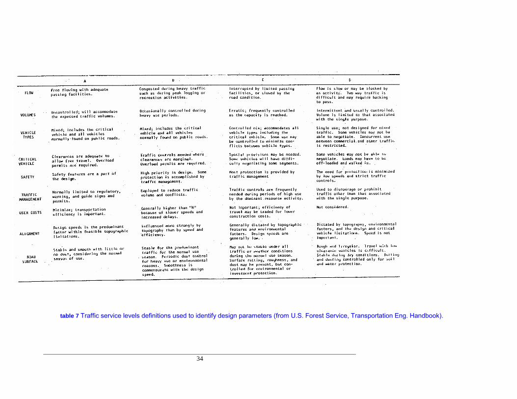
5. Traffic service level: This defines the type of traffic that will make use of the road network and itscharacteristics. Table 3 lists descriptions of four different levels of traffic service for forest roads. Eachlevel describes the traffic characteristics which are significant in the selection of design criteria anddescribe the operating conditions for the road. Each level also reflects a number of factors, such asspeed, travel time, traffic interruptions, freedom to maneuver, safety, driver comfort, convenience, andoperating cost. Traffic density is a factor only if heavy non-logging traffic is expected. These factors, inturn, affect: (1) number of lanes, (2) turnout spacing, (3) lane widths, (4) type of driving surface, (5) sightdistances, (6) design speed, (7) clearance, (8) horizontal and vertical alignment, (9) curve widening, (10)turn-arounds.

6. Vehicle characteristics: The resource management objectives, together with traffic requirements and trafficservice level criteria selected above, will define the types of vehicles that are to use the proposed road.Specific vehicle characteristics need to be defined since they will determine the "design standards" to beadopted when proceeding to the road design phase. The land manager has to distinguish between the"design vehicle" and the "critical vehicle". The design vehicle is a vehicle that ordinarily uses the road,such as dual axle flatbed trucks in the case of ranching or farming operations, or dump trucks in the caseof a mining operation. The critical vehicle represents a vehicle which is necessary for the contemplatedoperation (for instance, a livestock truck in the case of transporting range livestock) but uses the roadinfrequently. Here, the design should allow for the critical vehicle to pass the road with assist vehicles, ifnecessary, but without major delays or road reconstruction.

7. Safety: Traffic safety is an important requirement especially where multiple user types will be utilizing thesame road. Safety requirements such as stopping distance, sight distance, and allowable design speedcan determine the selected road standards in combination with the other design criteria.

8. Road uses: The users of the contemplated road should be defined by categories. For example, timberharvest activities will include all users related to the planned timber harvest, such as silviculturists,foresters, engineers, surveyors, blasting crews, and construction and maintenance crews, as well as thelogging crews. Administrative users may include watershed management specialists, wildlife or fisheriesbiologists, or ecologists, as well as foresters. Agricultural users would include stock herders and

32

rangeland management specialists and will have a different set of objectives than timber objectives. Anestimate of road use for each category is then made (e.g., numbers of vehicles per day). For eachcategory, the resource management objective over several planning horizons should be indicated. Forinstance, a road is to be built first for (1) the harvest of timber from a tract of land, then (2) access for thelocal population for firewood cutting or grazing, and finally (3) access for administration of watershedrehabilitation activities. The planner should determine if the road user characteristics would change overthe life of the road.

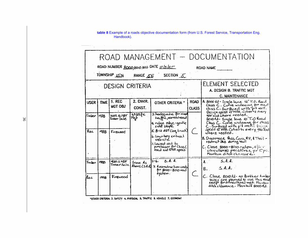
9. Economics: The various road alternatives would undergo rigorous economic evaluation.

As part of this process a "roads objectives documentation" plan should be carried out. This processconsists of putting the road management objectives and design criteria in an organized form. An example ofsuch a form is given in Table 4.

33

34

table 7 Traffic service levels definitions used to identify design parameters (from U.S. Forest Service, Transportation Eng. Handbook).

35

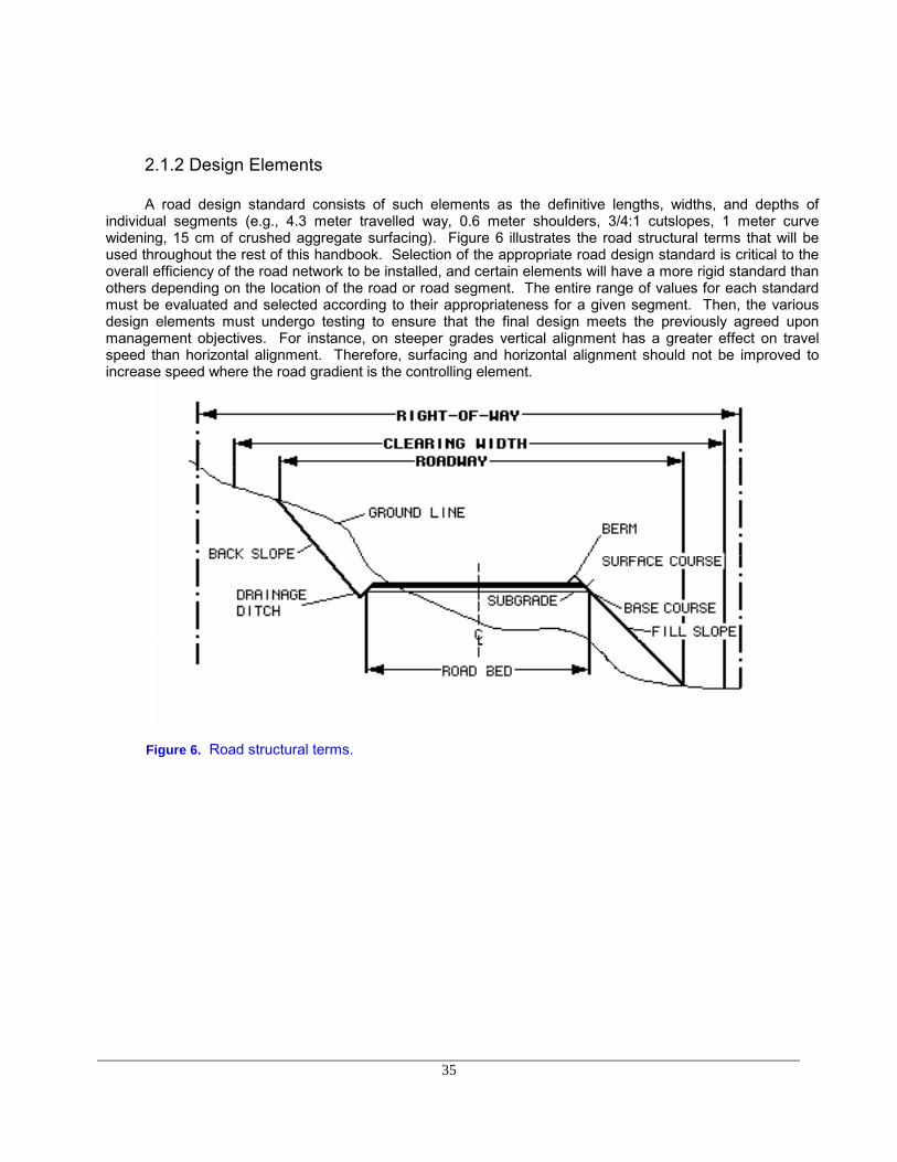
2.1.2 Design Elements

A road design standard consists of such elements as the definitive lengths, widths, and depths ofindividual segments (e.g., 4.3 meter travelled way, 0.6 meter shoulders, 3/4:1 cutslopes, 1 meter curvewidening, 15 cm of crushed aggregate surfacing). Figure 6 illustrates the road structural terms that will beused throughout the rest of this handbook. Selection of the appropriate road design standard is critical to theoverall efficiency of the road network to be installed, and certain elements will have a more rigid standard thanothers depending on the location of the road or road segment. The entire range of values for each standardmust be evaluated and selected according to their appropriateness for a given segment. Then, the variousdesign elements must undergo testing to ensure that the final design meets the previously agreed uponmanagement objectives. For instance, on steeper grades vertical alignment has a greater effect on travelspeed than horizontal alignment. Therefore, surfacing and horizontal alignment should not be improved toincrease speed where the road gradient is the controlling element.

Figure 6. Road structural terms.

36

table 8 Example of a roads objective documentation form (from U.S. Forest Service, Transportation Eng.Handbook).

37

2.1.2.1 Number of Lanes and Lane WidthThe majority of forest development road systems in the world are single-lane roads with turnouts. It is

anticipated that most roads to be constructed or reconstructed will also be single-lane with turnouts becauseof the continuing need for low volume, low speed roads and their desirability from economic andenvironmental impact standpoints. In choosing whether to build a single- or double-lane road, use the bestavailable data on expected traffic volumes, accident records, vehicle sizes, and season and time-of-day ofuse. Historically, the United States Forest Service has used traffic volumes of approximately 100 vehicles perday to trigger an evaluation for increasing road width from one to two lanes. Considering a day to consist of10 daylight hours, traffic volumes greater than 250 vehicles per day ordinarily require a double-lane road forsafe and efficient operation. Intermediate traffic volumes (between 100 and 250 vehicles per day) generallyrequire decisions based on additional criteria to those listed above: (1) social/political concerns, (2)relationships to public road systems, (3) season of use, (4) availability of funding, and (5) traffic management.

Many of the elements used in such an evaluation, although subjective, can be estimated using trafficinformation or data generated from existing roads in the area. For instance, if heavy public use of the road isanticipated, a traffic count on a comparably situated existing road will serve as a guide to the number ofvehicles per hour of non-logging traffic. Some elements can be evaluated in terms of relative probabilities andconsequences and can be identified as having a low, moderate, or high probability of occurrence and havingminor, moderate, or severe consequences. The more criteria showing higher probabilities and more severeconsequences, the stronger the need for a double-lane road.

2.1.2.2 Road widthThe primary consideration for determining the basic width of the roadbed is the types of vehicles

expected to be utilizing the road. Secondary considerations are the general condition of the traveled way,design speed, and the presence or absence of shoulders and ditches. Tables 5 and 6 list recommendedwidths for single- and double-lane roads, respectively.

table 9 Traveled way widths for single-lane roads.

-------------------------------------------------------------------------------------------------------------------------Type and Size Design Speed (Km/Hr)

of Vehicle --------------------------------------------------------30 40 50

-------------------------------------------------------------------------------------------------------------------------Minimum Traveled Way Width (m)

--------------------------------------------------------Recreational, administrative andservice vehicle, 2.0 to 2.4 m wide 3.0 3.0 3.6

Commercial hauling and commercialpassenger vehicles, including buses2.4 m wide or greater1. Road with ditch, or without ditch where cross slope is 3.6 3.6 4.2 25% or less

2. Roads without ditch where ground cross slope is greater than 25%. 3.6 3.6 4.2 The steepness of roadway backslope should be considered to provide adequate clearance.

----------------------------------------------------------------------------------------------------------------------

38

The presence of a ditch permits a narrower traveled way width since the ditch provides the necessaryclearance on one side. Except for additional widths required for curve widening, limit traveled way widths inexcess of 4.4 m (14 ft) to roads needed to accommodate off-highway haul and other unusual design vehicles.Double-lane roads designed for off-highway haul (all surface types) should conform to the following standards:

table 10 Lane widths for double-lane roads

---------------------------------------------------------------------------------------------------------------------------------------Size and Type Type Type Design Speed (Km/Hr)of Vehicle of Road of Surface---------------------------------------------------

15 30 45 60 80---------------------------------------------------------------------------------------------------------------------------------------

Minimum Lane Width (m)---------------------------------------------------

Recreational,adm. and service:1. up to 2.0 m wide Recreation or All surface 2.7 2.7 3.0 3.3 3.02. 2.0 to 2.4 m wide administrative types 3.0 3.0 3.3 3.3 3.3

Commercial hauling Roads open to Gravel - 3.3 3.6 3.6 -and comm. passenger truck traffic or nativevehicles incl. buses or mixed2.4 m wide or greater traffic Bituminous - 3.3 3.3 3.3 3.6

---------------------------------------------------------------------------------------------------------------------------------------Gravel or native surface roads should not have design speeds greater than 60 km/hrAdditional width is required for lower quality surfaces, because of the off-trackingcorrections needed compared to a higher quality surface.

Vehicles wider than the design vehicle (a "critical vehicle") may make occasional use of the road.Check traveled way and shoulder widths to ensure that these vehicles can safely traverse the road. Criticalvehicles should never attempt to traverse the road at or even approaching the speeds of the design vehicle.

Shoulders may be necessary to provide parking areas, space for installations such as drainagestructures, guardrails, signs, and roadside utilities, increase in total roadway width to match the clear width ofan opening for a structure such as a bridge or tunnel, a recovery zone for vehicles straying from the traveledway, additional width to accommodate a "critical vehicle", lateral support for outside edge of asphalt orconcrete pavements (0.3 m is sufficient for this purpose). The space required for these features will dependon the design criteria of the road and/or the design of specific structures to be incorporated as part of theroadway.

Minimum Width of Traveled Wayfor Design Speed

----------------------------------------------------------------------------------------------------------------------------Bunk Width 30 km/hr(20 mph) 50 km/hr (30 mph) 60 km/hr (40 mph)

3 .0m (10 ft) 6.7 m (22 ft) 7.3 m (24 ft) 7.9 m (26 ft)3.7 m (12 ft) 7.9 m (26 ft) 8.5 m (28 ft) 8.5 m (28 ft)----------------------------------------------------------------------------------------------------------------------------

39

2.1.2.3. TurnoutsTurnout spacing, location, and dimensions provide user convenience and safety and allow vehicles to

maintain a reasonable speed. Spacing can be computed using the following formula and the curves fromFigure 7 and Table 7 :

T = 1.609*(DS)/36

Where: T = Increase in travel time for the interrupted vehicle (percent) D = Delay time per kilometer for the interrupted vehicle (seconds) S = Design speed (kilometers per hour).

Solve the equation for T and then use the graph in Figure 7 to determine the turnout spacing required toaccommodate the number of vehicles passing over the road per hour (VPH).

Figure 7. Turnout spacing in relation to traffic volume and travel delay time.

Figure 8 illustrates a typical turnout in detail. Turnouts should be located on the outside of cuts, thelow side of fills, or at the runout point between through cuts and fills, and preferably on the side of theunloaded vehicle. Table 8 gives recommended turnout widths and lengths for various traffic service levels.The maximum transition length should be limited to 22.5 m for all service levels.

table 11 Recommended turnout spacing--all traffic service levels

40

---------------------------------------------------------------------------------------------------------------------------------------Traffic OperationalService Turnout Spacing Constraints---------------------------------------------------------------------------------------------------------------------------------------

Make turnouts intervisible unless Traffic: Mixedexcessive costs or environmental Capacity: Up to 25 vehicles per hourconstraints preclude construction Design Speed: Up to 60 km/hr

A Closer spacing may contribute Delays: 12 sec./km or lessto efficiency and convenience.Maximum spacing is 300 m.

Intervisible turnouts are highly Traffic: Mixeddesirable but may be precluded Capacity: Up to 25 vehicles per hour

B by excessive costs or environmental Design Speed: Up to 40 km/hrconstraints. Maximum spacings Delays: 20 km/hr or less300 m. Use signs to warn non-commercial

users of traffic to be expected. Roadsegments without intervisible turn-outs should be signaled.

Maximum spacing is 300 m. Traffic: Small amount of mixedWhen the environmental impact is Capacity: Up to 20 vehicles per hourlow and the investment is economi- Design Speed: Up to 30 km/hr

C cally justifiable, additional turn- Delays: Up to 40 sec./kmouts may be constructed. Roads should be managed to minimize

conflicts between commercialand non-commercial users.

Generally, only naturally occurring Traffic: Not intended for mixedD turnouts, such as on ridges or Capacity: Generally 10 VPH or less

other available areas Design Speed: 25 km/hr or lesson flat terrain, are used. Delays: At least 45 sec./km expected.

Road should be managed to restrictconcurrent use by commercial andnon-commercial users.

---------------------------------------------------------------------------------------------------------------------------------------

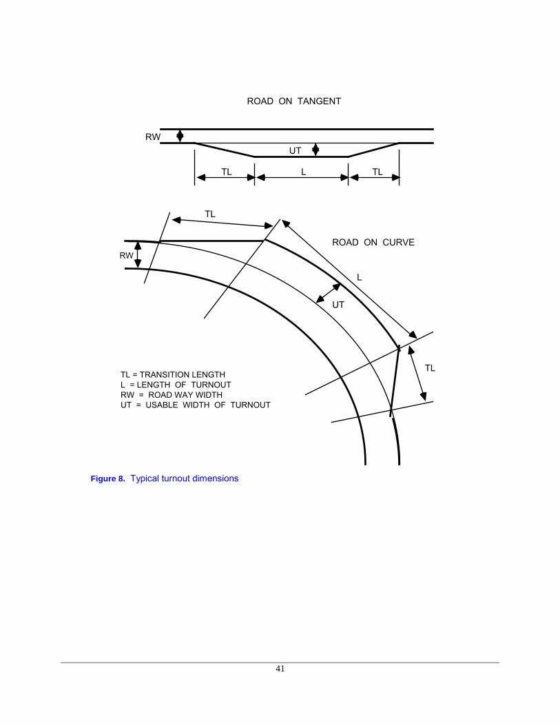
41

ROAD ON TANGENT

RWUT

TL L TL

RW

TL

L

UT

TL

ROAD ON CURVE

TL = TRANSITION LENGTH L = LENGTH OF TURNOUT RW = ROAD WAY WIDTH UT = USABLE WIDTH OF TURNOUT

Figure 8. Typical turnout dimensions

42

table 12 Turnout widths and lengths

----------------------------------------------------------------------------------------------------------------------------------Traffic Service Turnout Width Turnout Length &

Levels Transition Length----------------------------------------------------------------------------------------------------------------------------------

Design vehicle length orA 3.0 m 22.5 m minimum, whichever

is largest.Minimum 15 m transition at each end.

Design vehicle length.B 3.0 m Minimum 15 m transition

at each end.

Make the minimum total Empty truck lengthwidth of the traveled way and (trailer loaded on truck)

D turnout the width of two Minimum 7.5 m transitionsdesign vehicles plus 1.2 m at each end.

----------------------------------------------------------------------------------------------------------------------------------

2.1.2.4. Turn-aroundsTurn-around design should consider both critical and design vehicles and should be provided at or

near the end of single-lane roads, and at management closure points, such as gates or barricades. Ifintermediate turn-arounds are necessary, signing should be considered if they create a hazard to otherusers. The turn-around should be designed to allow the design vehicle to turn with reasonably safemaneuvering.

2.1.2.5. Curve WideningWidening may be required on some curves to allow for off-tracking of tractor-trailer vehicles and for

some light vehicle-trailer combinations. Widening of the traveled way on curves to accommodate the designvehicle is considered a part of the traveled way. Generally, the need for curve widening increases as curveradius decreases with shorter curves requiring less curve widening than longer curves. Criteria forestablishing the need for curve widening given traffic service levels are given in Table 9.

table 13 Curve widening criteria

-------------------------------------------------------------------------------------------------------------------------------------TrafficService Curve WideningLevel

--------------------------------------------------------------------------------------------------------------------------------------A Design curve widening to accommodate the design vehicle (normally low-boy) at the design

speed for each curve. Curve widening for critical vehicles to be provided by the use of otherroad elements, if planned, such as turnouts and shoulders. Provide widening if needed widthis not available. Critical vehicle should be accommodated in its normal travelingconfiguration. Curve widening to be provided in each lane of double-lane roads.

B Same as A.

C Same as A, except the critical vehicle configuration may need alteration.

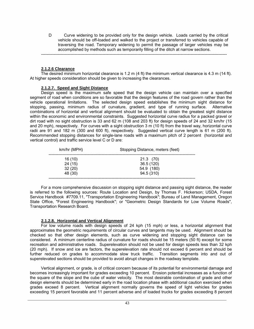
43

D Curve widening to be provided only for the design vehicle. Loads carried by the criticalvehicle should be off-loaded and walked to the project or transferred to vehicles capable oftraversing the road. Temporary widening to permit the passage of larger vehicles may beaccomplished by methods such as temporarily filling of the ditch at narrow sections.

-------------------------------------------------------------------------------------------------------------------------------------

2.1.2.6 ClearanceThe desired minimum horizontal clearance is 1.2 m (4 ft) the minimum vertical clearance is 4.3 m (14 ft).

At higher speeds consideration should be given to increasing the clearances.

2.1.2.7. Speed and Sight DistanceDesign speed is the maximum safe speed that the design vehicle can maintain over a specified

segment of road when conditions are so favorable that the design features of the road govern rather than thevehicle operational limitations. The selected design speed establishes the minimum sight distance forstopping, passing, minimum radius of curvature, gradient, and type of running surface. Alternativecombinations of horizontal and vertical alignment should be evaluated to obtain the greatest sight distancewithin the economic and environmental constraints. Suggested horizontal curve radius for a packed gravel ordirt road with no sight obstruction is 33 and 62 m (108 and 203 ft) for design speeds of 24 and 32 km/hr (15and 20 mph), respectively. For curves with a sight obstruction 3 m (10 ft) from the travel way, horizontal curveradii are 91 and 182 m (300 and 600 ft), respectively. Suggested vertical curve length is 61 m (200 ft).Recommended stopping distances for single-lane roads with a maximum pitch of 2 percent (horizontal andvertical control) and traffic service level C or D are:

km/hr (MPH) Stopping Distance, meters (feet)---------------------------------------------------------------------------------------------------------

16 (10) 21.3 (70)24 (15) 36.5 (120)32 (20) 54.9 (180)48 (30) 94.5 (310)

---------------------------------------------------------------------------------------------------------

For a more comprehensive discussion on stopping sight distance and passing sight distance, the readeris referred to the following sources: Route Location and Design, by Thomas F. Hickerson; USDA, ForestService Handbook #7709.11, "Transportation Engineering Handbook"; Bureau of Land Management, OregonState Office, "Forest Engineering Handbook"; or "Geometric Design Standards for Low Volume Roads",Transportation Research Board.

2.1.2.8. Horizontal and Vertical AlignmentFor low volume roads with design speeds of 24 kph (15 mph) or less, a horizontal alignment that

approximates the geometric requirements of circular curves and tangents may be used. Alignment should bechecked so that other design elements, such as curve widening and stopping sight distance can beconsidered. A minimum centerline radius of curvature for roads should be 15 meters (50 ft) except for somerecreation and administrative roads. Superelevation should not be used for design speeds less than 32 kph(20 mph). If snow and ice are factors, the superelevation rate should not exceed 6 percent and should befurther reduced on grades to accommodate slow truck traffic. Transition segments into and out ofsuperelevated sections should be provided to avoid abrupt changes in the roadway template.

Vertical alignment, or grade, is of critical concern because of its potential for environmental damage andbecomes increasingly important for grades exceeding 10 percent. Erosion potential increases as a function ofthe square of the slope and the cube of water velocity. The most desirable combination of grade and otherdesign elements should be determined early in the road location phase with additional caution exercised whengrades exceed 8 percent. Vertical alignment normally governs the speed of light vehicles for gradesexceeding 15 percent favorable and 11 percent adverse and of loaded trucks for grades exceeding 8 percent

44

favorable and 3 percent adverse. The ability of a vehicle to traverse a particular grade is dependent on vehicleweight and horsepower and on the traction coefficient of the driving surface.

Travel time and cost are affected by horizontal alignment, such as curve radius and road width. Figure9 shows the relationship between average truck speed and curve radius for several road widths. For example,there is a 15 percent difference in average truck speed on a 30.5 m (100 ft) radius curve for a 3.7 m wide roadwhen compared to a 4.3 m wide road.

Horizontal alignment has been classified on the basis of curve radius and number of curves. The U. S.Forest Service, for example, uses the following classification system:

[Average radius (m)] / [# of curves / km]---------------------------------------------------------------------------------------------------------

Poor = < 4 Good = 10 - 20Fair = 4 - 10 Excellent = > 20

---------------------------------------------------------------------------------------------------------

The effect of grade on truck speed (loaded and unloaded) is shown in Figure 10. The speed of aloaded truck is most sensitive to grade changes from 0 to 7 percent in the direction of haul. For gradessteeper than 7 percent other considerations are more important than impact on speed.

0

5

10

15

20

25

30

15 50 100 150 200 250 300

SINGLE LANE; 3.7m road w/oditch

Single Lane; 4.3m road with 1mditch

Lane-and-one-half; 6m road&1.2m ditch

Double Lane Road

AVERAGE TRUCK SPEEDTHROUGH CURVE

RADIUS OF CURVE (METERS)

SPEED (KM/HR)

Figure 9. Relationship between curve radius and truck speed when speed is not controlled bygrade.

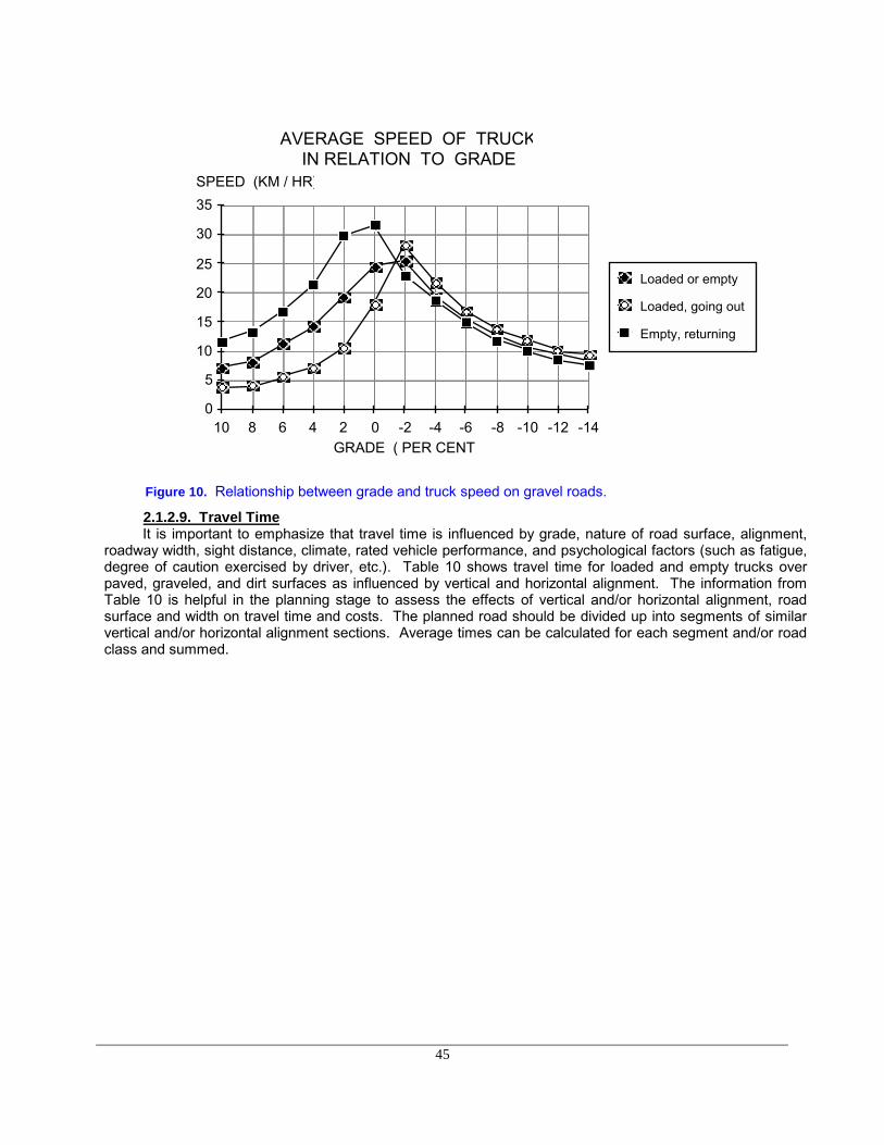
45

0

5

10

15

20

25

30

35

10 8 6 4 2 0 -2 -4 -6 -8 -10 -12 -14

Loaded or empty

Loaded, going out

Empty, returning

AVERAGE SPEED OF TRUCKIN RELATION TO GRADE

GRADE ( PER CENT

SPEED (KM / HR)

Figure 10. Relationship between grade and truck speed on gravel roads.

2.1.2.9. Travel TimeIt is important to emphasize that travel time is influenced by grade, nature of road surface, alignment,

roadway width, sight distance, climate, rated vehicle performance, and psychological factors (such as fatigue,degree of caution exercised by driver, etc.). Table 10 shows travel time for loaded and empty trucks overpaved, graveled, and dirt surfaces as influenced by vertical and horizontal alignment. The information fromTable 10 is helpful in the planning stage to assess the effects of vertical and/or horizontal alignment, roadsurface and width on travel time and costs. The planned road should be divided up into segments of similarvertical and/or horizontal alignment sections. Average times can be calculated for each segment and/or roadclass and summed.

46

table 14 Relationship between round trip travel time per kilometer and surface type as influenced by verticaland horizontal alignment; adverse grade in direction of haul (U.S. Forest service, 1965).

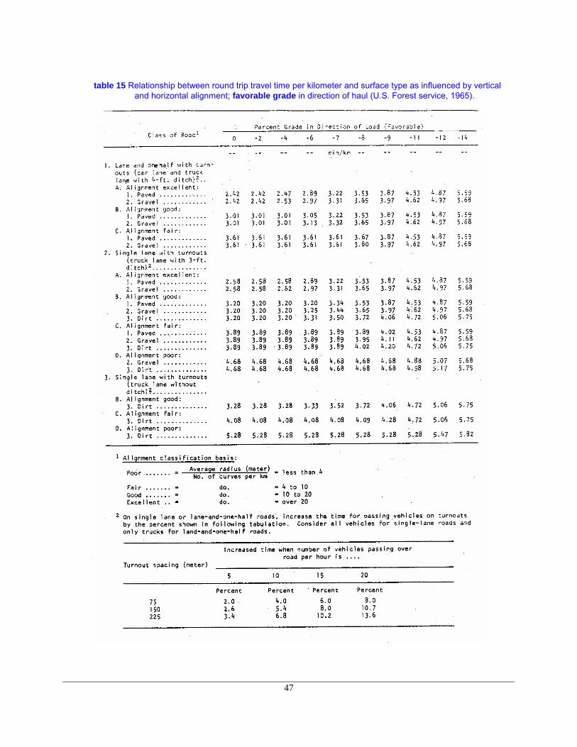
47

table 15 Relationship between round trip travel time per kilometer and surface type as influenced by verticaland horizontal alignment; favorable grade in direction of haul (U.S. Forest service, 1965).

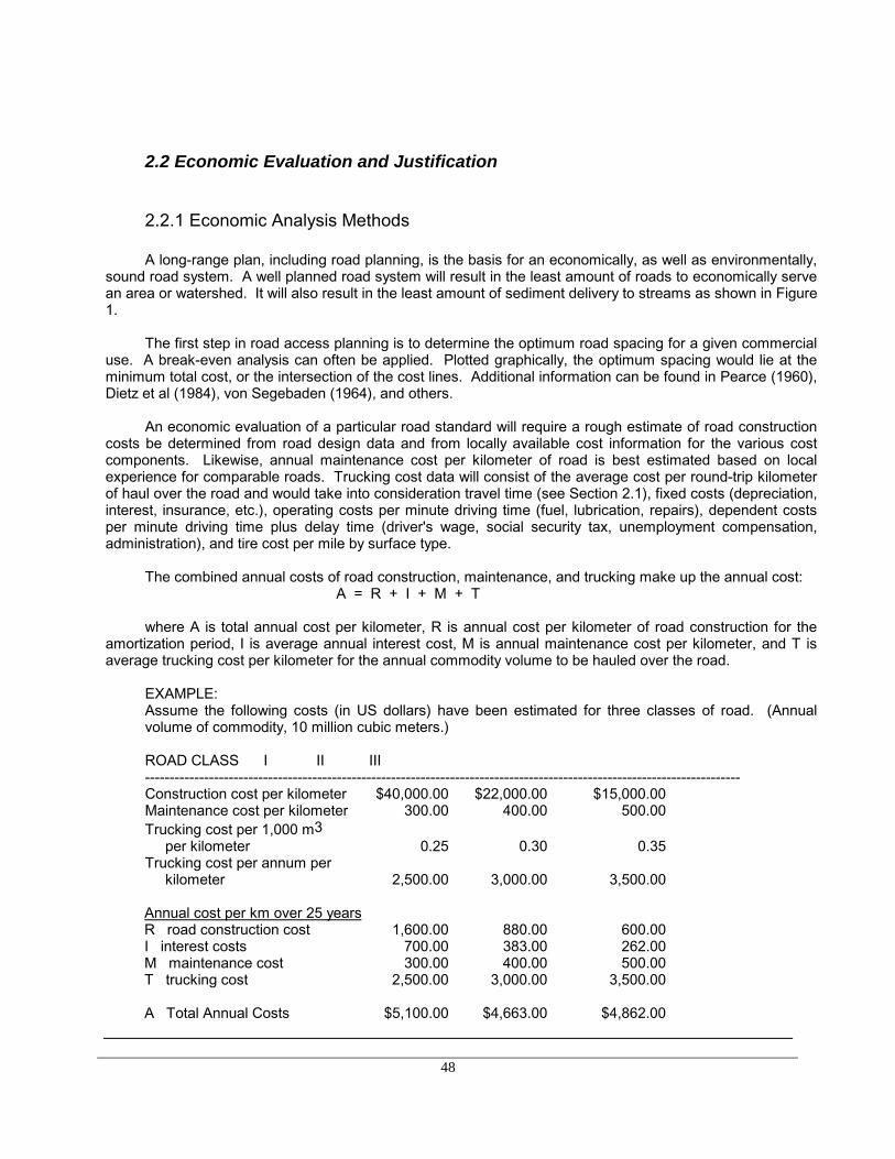
48

2.2 Economic Evaluation and Justification

2.2.1 Economic Analysis Methods

A long-range plan, including road planning, is the basis for an economically, as well as environmentally,sound road system. A well planned road system will result in the least amount of roads to economically servean area or watershed. It will also result in the least amount of sediment delivery to streams as shown in Figure1.

The first step in road access planning is to determine the optimum road spacing for a given commercialuse. A break-even analysis can often be applied. Plotted graphically, the optimum spacing would lie at theminimum total cost, or the intersection of the cost lines. Additional information can be found in Pearce (1960),Dietz et al (1984), von Segebaden (1964), and others.

An economic evaluation of a particular road standard will require a rough estimate of road constructioncosts be determined from road design data and from locally available cost information for the various costcomponents. Likewise, annual maintenance cost per kilometer of road is best estimated based on localexperience for comparable roads. Trucking cost data will consist of the average cost per round-trip kilometerof haul over the road and would take into consideration travel time (see Section 2.1), fixed costs (depreciation,interest, insurance, etc.), operating costs per minute driving time (fuel, lubrication, repairs), dependent costsper minute driving time plus delay time (driver's wage, social security tax, unemployment compensation,administration), and tire cost per mile by surface type.

The combined annual costs of road construction, maintenance, and trucking make up the annual cost: A = R + I + M + T

where A is total annual cost per kilometer, R is annual cost per kilometer of road construction for theamortization period, I is average annual interest cost, M is annual maintenance cost per kilometer, and T isaverage trucking cost per kilometer for the annual commodity volume to be hauled over the road.

EXAMPLE:Assume the following costs (in US dollars) have been estimated for three classes of road. (Annualvolume of commodity, 10 million cubic meters.)

ROAD CLASS I II III-------------------------------------------------------------------------------------------------------------------------Construction cost per kilometer $40,000.00 $22,000.00 $15,000.00Maintenance cost per kilometer 300.00 400.00 500.00Trucking cost per 1,000 m3 per kilometer 0.25 0.30 0.35Trucking cost per annum per kilometer 2,500.00 3,000.00 3,500.00

Annual cost per km over 25 yearsR road construction cost 1,600.00 880.00 600.00I interest costs 700.00 383.00 262.00M maintenance cost 300.00 400.00 500.00T trucking cost 2,500.00 3,000.00 3,500.00

A Total Annual Costs $5,100.00 $4,663.00 $4,862.00

49

(If amortization period is 25 years, the annual rate is 4 percent of the construction cost. If theinterest rate is 3.5 percent, the average annual interest rate is 1.75 percent.)

Note that in the above calculation the Class II road is the most economical by a margin of $199.00 overthe Class III road. Over the period of amortization of 25 years, the margin for the Class II road will be$4,975.00 per kilometer.

Another method in choosing the most economical of two road standards is to calculate the annualamount or volume of commodity at which the costs of the two roads will be equal. If annual volume exceedsthe calculated amount the higher road standard will be justified; likewise, if annual volume is less than thecalculated amount, the lower standard is justified. The formula for calculating V is:

(R + I + M)H - (R + I + M)LV = ------------------------------------------

TL - TH

The subscripts H and L indicate high and low standard, respectively, and T is expressed as cost per1000 m3 per kilometer. All other values are expressed in units stated above.

EXAMPLE

Using the same costs as in the previous example for the Class II and Class III road, the annualvolume is calculated as:

(880 + 383 + 400) - (600 + 262 + 500)V = ------------------------------------------------------------------ = 6,020 x 103 m3

(0.35 - 0.30)

Hence, for volumes exceeding 6.02 x 106 m3 the Class II road is the more economical choice; forvolumes less than 6.02 x 106 m3 the Class III road would be chosen. If the two roads differ in length, multiplythe costs per kilometer by the number of kilometers of each road for use in this formula.

2.2.2 Analysis of Alternative Routes

The above formulas can also be used to evaluate two or more alternatives to a proposed route. Onecommon situation is to choose between a longer route on a gentle favorable grade and a shorter routeinvolving an adverse grade and a steeper favorable grade.

EXAMPLE.

1. Longer route segment: 3.67 km of 3% favorable grade. Trucking cost = $.562 per 1000 m3; constructioncost $55,050 at 6% amortization plus interest = $3,303; annual maintenance at$300/km = $1,101. Total annual cost = $4,404.

2. Shorter route segment: 2.0 km of 8% favorable grade, 1 km of 5% adverse grade. Trucking cost = $.81per 1000 m3; construction cost $41,000 at 6% amortization plus interest = $2,460;annual maintenance at $400/km (steeper grade, sharper curves) = $1,200. Total annual cost = $3,660.

V = (4,404 - 3,660)/(0.81 - 0.562) = 3 x 106 m3

(According to the formula, the longer route will be the more economical if the annual volume hauledexceeds 3 million cubic meters.)

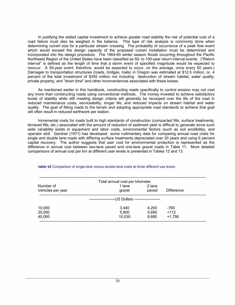
50

In justifying the added capital investment to achieve greater road stability the risk of potential cost of aroad failure must also be weighed in the balance. This type of risk analysis is commonly done whendetermining culvert size for a particular stream crossing. The probability of occurrence of a peak flow eventwhich would exceed the design capacity of the proposed culvert installation must be determined andincorporated into the design procedure. The 1964-65 winter season floods occurring throughout the PacificNorthwest Region of the United States have been classified as 50- to 100-year return interval events. ("Returninterval" is defined as the length of time that a storm event of specified magnitude would be expected toreoccur. A 50-year event, therefore, would be expected to occur, on the average, once every 50 years.)Damages to transportation structures (roads, bridges, trails) in Oregon was estimated at $12.5 million, or, 4percent of the total investment of $355 million not including destruction of stream habitat, water quality,private property, and "down time" and other inconveniences associated with these losses.

As mentioned earlier in this handbook, constructing roads specifically to control erosion may not costany more than constructing roads using conventional methods. The money invested to achieve satisfactorylevels of stability while still meeting design criteria will generally be recouped over the life of the road inreduced maintenance costs, serviceability, longer life, and reduced impacts on stream habitat and waterquality. The goal of fitting roads to the terrain and adopting appropriate road standards to achieve that goalwill often result in reduced earthwork per station.

Incremental costs for roads built to high standards of construction (compacted fills, surface treatments,terraced fills, etc.) associated with the amount of reduction of sediment yield is difficult to generate since suchwide variability exists in equipment and labor costs, environmental factors (such as soil erodibility), andoperator skill. Gardner (1971) has developed some rudimentary data for comparing annual road costs forsingle and double lane roads with differing surface treatments depreciated over 20 years and using 6 percentcapital recovery. The author suggests that user cost for environmental protection is represented as thedifference in annual cost between two-lane paved and one-lane gravel roads in Table 11. More detailedcomparisons of annual cost per km at different user levels is presented in Tables 12 and 13.

table 16 Comparison of single-lane versus double-lane costs at three different use levels.

---------------------------------------------------------------------------------------------------------------------------------Total annual cost per kilometer

Number of 1 lane 2 laneVehicles per year gravel paved Difference

-----------------------------------------------------------------------------------------------------------------------------------------------------US Dollars --------------------

10,000 3,440 4,200 -76020,000 5,800 5,690 +11240,000 10,530 8,680 +1,790

---------------------------------------------------------------------------------------------------------------------------------

51

table 17 Comparison of annual road costs per kilometer -- 10,000 vehicles per year.

________________________________________________________________Road Standard

Costdistribution 2 lane 2 lane 2 lane 1 lane 1 lane 1 lane

paved chip-seal gravel gravel spot stabilization primitive________________________________________________________________

----------------Dollars per kilometer-------------------InitialConstruction $31,070 $24,860 $18,640 $12,430 $9,320 $6,210

--------Dollars per kilometer per year (20-year period)-------Depreciation1 2,710 2,170 1,620 1,080 810 540Maintenance 120 250 370 500 680 310Vehicle use 1,370 1,430 1,680 1,860 2,730 5,280

Total annual 4,200 3,850 3,670 3,4402 4,230 6,130________________________________________________________________1 20 years at 6% using capital recovery.2 Lowest annual cost.

table 18 Comparison of annual road costs per kilometer for 20,000 and 40,000

vehicles per year--------------------------------------------------------------------------------------------------------------------------------

Road StandardCostdistribution 2 lane 2 lane 2 lane 1 lane 1 lane 1 lane

paved chip-seal gravel gravel spot stabilization primitive--------------------------------------------------------------------------------------------------------------------------------

----------------Dollars per kilometer-------------------Initialconstruction 31,070 24,860 18,640 12,430 9,320 6,210

--------Dollars per kilometer per year (20-year period)------- 20,000 vehicles per year

Depreciation1 2,710 2,170 1,620 1,080 810 540Maintenance 250 500 750 1,000 1,370 620Vehicle use 2,730 2,860 3,360 3,730 5,470 10,560

Total annual 5,690 5,5302 5,730 5,810 7,650 11,720

--------Dollars per kilometer per year (20-year period)------- 40,000 vehicles per year

Depreciation 2,710 2,170 1,620 1,080 810 540Maintenance 500 1,000 1,490 1,990 2,730 1,240Vehicle use 5,470 5,720 6,710 7,460 10,940 21,130

Total annual 8,6802 8,890 9,820 10,530 14,480 22,910---------------------------------------------------------------------------------------------------------------------------------1 20 years at 6% using capital recovery.2 Lowest annual cost.

52

Gardner (1978) analyzed alternative design standards and costs in addition to observing the initialperformance of the experimental road and its esthetic acceptability. Alternate design features includedreducing road width to a level that would accommodate the tracks of the proposed yarding equipment (3.81 m(12.5 ft)), treating slash by chipping and scattering below the toe of the fill, using turnouts only when the terrainwas favorable thus keeping road widths to a minimum, creating stepped backslopes (Figure 11 ) wherebedrock competence was good and planting shrubs and grasses with and without straw mulches, and, finally,incorporating neoprene down- spouts below culverts to dissipate energy and protect the road prism. SectionsI and II of the experimental road had the following characteristics:

Average grade Average curve radius # curves / km (mi) ( percent ) ( meters )

---------------------------------------------------------------------------------------------------------------------------Section I 7.26 25.00 12.1 (19.4)Section II 5.90 19.30 10.8 (17.4)

Figure 11 Stepped backslope (no scale).

Gardner found that using 1/10:1 backslopes and reducing clearing widths in the experimental roadsaved approximately $4,333 in construction cost and had no adverse effect on logging or hauling cost (Table14). The effects on harvesting costs were not analyzed in this study.

53

table 19 Cost summary comparison (5 vehicles per hour--1/2 logging trucks, 1/2 other traffic); assumes 8-hour hauling day, 140 days/year use, 20 year road life, 23.8 m3 (6.0 M bd. ft.) loads for loggingtrucks, cost of operating logging trucks including driver's wage--$0.25/min, cost of operating othervehicles--$0.04/minute, 5,535 m3 (1 1/2 MM bd. ft.) timber harvested. (Gardner, 1978)

----------------------------------------------------------------------------------------------------------------------------------Annual

amortized Annual AnnualRoad difference difference difference Netstandard* in cost hauling cost other traffic difference----------------------------------------------------------------------------------------------------------------------------------

-------------------Dollars-----------------------Experimental 0III +1,842.99 -3,187.65 -431.20 -1,775.86IV +11,790.22 -15,287.59 -2,371.60 -5,868.97---------------------------------------------------------------------------------------------------------------------------------* Experimental road: single lane, 4.27 m (14 ft) width, 24.1 kph (15 mph) design speed, 0.91 m (3 ') ditch. III road: single lane, 4.88 m (16 ft) width, 27.4 km/hr (17 mph) design speed, 0.91 m (3 ft) ditch. IV road: double lane, 7.32 m (24 ft) width, 38.6 km/hr (24 mph) design speed, 1.22 m (4 ft) ditch.

Table 14 indicates that any environmental values gained by the construction of the experimental roadwould cause little economic sacrifice at vehicle use levels of 5 per hour. At higher use levels, however, thetrade-offs become more significant and decisions regarding standards become more difficult.

54

2.3 Route Reconnaissance and Location

Keep in mind that a bad road in a good location is preferable to a good road in a bad location. A badroad can nearly always be fixed. However, no amount of quality survey or design work can correct anysignificant location error. For instance, a road constructed across a steep headwall area is more likely tointercept surface and subsurface water flow and has a far greater potential for failure than a road constructedalong the ridgeline above the headwall. Since excess moisture is nearly always associated with landslides, itis always best to avoid drainage areas where water is expected to collect. Some important factors toremember when locating roads include:

1. Avoid high erosion hazard sites, particularly where mass failure is a possibility.

2. Utilize natural terrain features such as stable benches, ridgetops, and low gradient slopes to minimize thearea of road disturbance.

3. f necessary, include short road segments with steeper gradients to avoid problem areas or to utilizenatural terrain features.

4. Avoid midslope locations on long, steep, or unstable slopes.

5. Locate roads on well-drained soils and rock formations which dip into slopes rather than areascharacterized by seeps, highly plastic clays, concave slopes hummocky topography, cracked soil and rockstrata dipping parallel to the slope.

6. For logging road, utilize natural log landing areas (flatter, benched, well-drained land) to reduce soildisturbance associated with log landings and skid roads.

7. Avoid undercutting unstable, moist toe slopes when locating roads in or near a valley bottom.

8. Roll or vary road grades where possible to dissipate flow in road drainage ditches and culverts and toreduce surface erosion.

9. Select drainage crossings to minimize channel disturbance during construction and to minimize approachcuts and fills.

10. Locate roads far enough above streams to provide an adequate buffer, or provide structure or objects tointercept sediment moving downslope below the road.

11. If an unstable area such as a headwall must be crossed, consider end hauling excavated material ratherthan using sidecast methods. Avoid deep fills and compact all fills to accepted engineering standards.Design for close culvert and cross drain spacing to effectively remove water from ditches and provide foradequate energy dissipators below culvert outlets. Horizontal drains or interceptor drains may benecessary to drain excess groundwater.

2.3.1 Road Reconnaissance

Erosion and sedimentation rates are directly linked to total road surface area and excavation. Thecloser the road centerline follows the natural topographic contour, the smaller the erosional impact will be. Onlow-volume roads it is permissible and even advisable to use non-geometric alignment standards, or the "freealignment method". The beauty of this system is its ability to permit design decisions to be made in the field

55

while allowing for tighter control in areas with critical grades and alignments such as draws, switchbacks,steep topography, or ridges, and less control in areas where resource risks are minimal. Clearing andexcavation quantities are substantially reduced compared to conventional geometric alignment methods.More time is spent "on the ground" in the road location step and preliminary survey so that major alignmentchanges are not necessary during the design phase.

The road locator runs two types of tag or grade line. On more gentle ground the tag or grade linefollows closely, or is identical to the proposed road centerline (Figure 12).

CL

Tag Line

Figure 12. Tag line location and centerline location of proposed road. Sideslopes are typically lessthan 40 to 50 percent.

On steeper ground where heavy cuts on centerline are required (sideslopes greater than 50 to 60percent), the tag line is marked on the "grade-out" or "daylight" point (Figure 13).

Tag Line

Grade-out or Daylight Point

CL

Figure 13. Tag line location and centerline location of proposed road. Sideslopes are typically 50%or steeper.

The following procedure has been proven to be successful for direct location of the centerline. First, thetag line is run with abney or clinometer. Tags, flagging, or ribbons are hung at eye level (approximately 150 to170 cm) above ground. The ribbon should be intervisible and hung every 15 to 25 m depending ontopography and vegetation density. Once a satisfactory tag line has been established, a second pass is mademarking tangents and points of intersection (PI) of tangent (Figure 14).

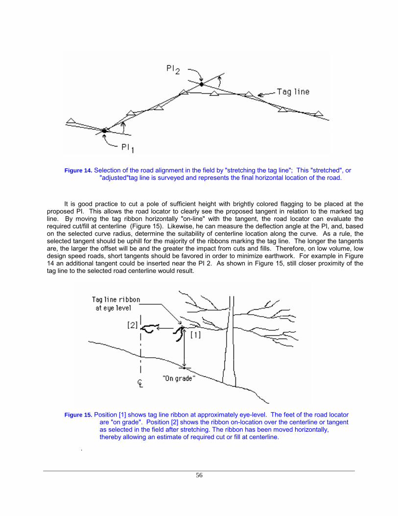
56

Figure 14. Selection of the road alignment in the field by "stretching the tag line"; This "stretched", or"adjusted"tag line is surveyed and represents the final horizontal location of the road.

It is good practice to cut a pole of sufficient height with brightly colored flagging to be placed at theproposed PI. This allows the road locator to clearly see the proposed tangent in relation to the marked tagline. By moving the tag ribbon horizontally "on-line" with the tangent, the road locator can evaluate therequired cut/fill at centerline (Figure 15). Likewise, he can measure the deflection angle at the PI, and, basedon the selected curve radius, determine the suitability of centerline location along the curve. As a rule, theselected tangent should be uphill for the majority of the ribbons marking the tag line. The longer the tangentsare, the larger the offset will be and the greater the impact from cuts and fills. Therefore, on low volume, lowdesign speed roads, short tangents should be favored in order to minimize earthwork. For example in Figure14 an additional tangent could be inserted near the PI 2. As shown in Figure 15, still closer proximity of thetag line to the selected road centerline would result.

Figure 15. Position [1] shows tag line ribbon at approximately eye-level. The feet of the road locatorare "on grade". Position [2] shows the ribbon on-location over the centerline or tangentas selected in the field after stretching. The ribbon has been moved horizontally,thereby allowing an estimate of required cut or fill at centerline.

.

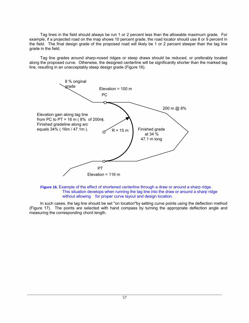
57

Tag lines in the field should always be run 1 or 2 percent less than the allowable maximum grade. Forexample, if a projected road on the map shows 10 percent grade, the road locator should use 8 or 9 percent inthe field. The final design grade of the proposed road will likely be 1 or 2 percent steeper than the tag linegrade in the field.

Tag line grades around sharp-nosed ridges or steep draws should be reduced, or preferably locatedalong the proposed curve. Otherwise, the designed centerline will be significantly shorter than the marked tagline, resulting in an unacceptably steep design grade (Figure 16).

200 m @ 8%

8 % original grade

PCElevation = 100 m

Finished grade at 34 %

47.1 m long

R = 15 m

PTElevation = 116 m

Elevation gain along tag line from PC to PT = 16 m ( 8% of 200m ). Finished gradeline along arc equals 34% ( 16m / 47.1m ).

Figure 16. Example of the effect of shortened centerline through a draw or around a sharp ridge.This situation develops when running the tag line into the draw or around a sharp ridgewithout allowing for proper curve layout and design location.

In such cases, the tag line should be set "on location"by setting curve points using the deflection method(Figure 17). The points are selected with hand compass by turning the appropriate deflection angle andmeasuring the corresponding chord length.

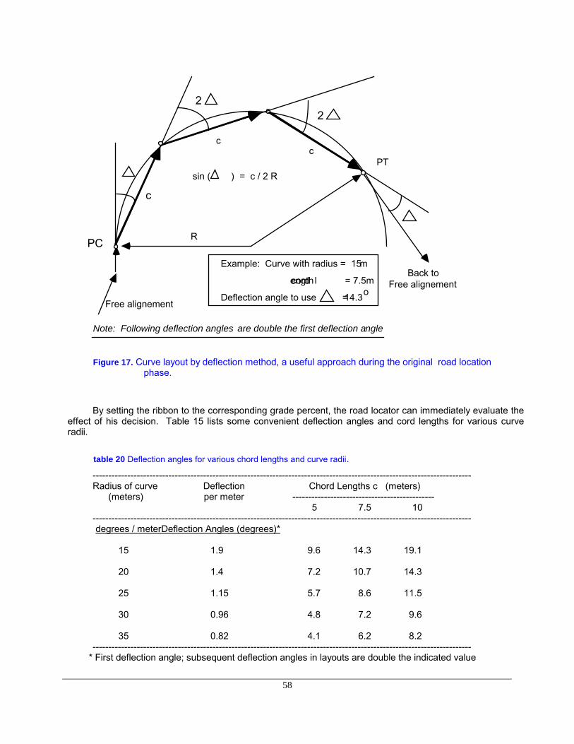
58

PC

PT

R

c

Back to Free alignement

Free alignement

sin ( ) = c / 2 R

Example: Curve with radius = 15 m

cord length = 7.5m

Deflection angle to use = 14.3o

Note: Following deflection angles are double the first deflection angle

cc

22

Figure 17. Curve layout by deflection method, a useful approach during the original road locationphase.

By setting the ribbon to the corresponding grade percent, the road locator can immediately evaluate theeffect of his decision. Table 15 lists some convenient deflection angles and cord lengths for various curveradii.

table 20 Deflection angles for various chord lengths and curve radii.

------------------------------------------------------------------------------------------------------------------------Radius of curve Deflection Chord Lengths c (meters)

(meters) per meter --------------------------------------------- 5 7.5 10

------------------------------------------------------------------------------------------------------------------------ degrees / meterDeflection Angles (degrees)*

15 1.9 9.6 14.3 19.1

20 1.4 7.2 10.7 14.3

25 1.15 5.7 8.6 11.5

30 0.96 4.8 7.2 9.6

35 0.82 4.1 6.2 8.2------------------------------------------------------------------------------------------------------------------------

* First deflection angle; subsequent deflection angles in layouts are double the indicated value

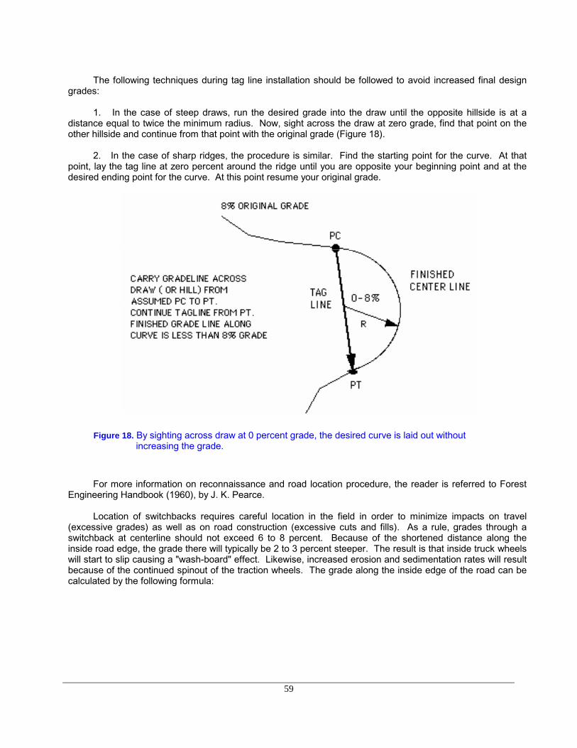
59

The following techniques during tag line installation should be followed to avoid increased final designgrades:

1. In the case of steep draws, run the desired grade into the draw until the opposite hillside is at adistance equal to twice the minimum radius. Now, sight across the draw at zero grade, find that point on theother hillside and continue from that point with the original grade (Figure 18).

2. In the case of sharp ridges, the procedure is similar. Find the starting point for the curve. At thatpoint, lay the tag line at zero percent around the ridge until you are opposite your beginning point and at thedesired ending point for the curve. At this point resume your original grade.

Figure 18. By sighting across draw at 0 percent grade, the desired curve is laid out withoutincreasing the grade.

For more information on reconnaissance and road location procedure, the reader is referred to ForestEngineering Handbook (1960), by J. K. Pearce.

Location of switchbacks requires careful location in the field in order to minimize impacts on travel(excessive grades) as well as on road construction (excessive cuts and fills). As a rule, grades through aswitchback at centerline should not exceed 6 to 8 percent. Because of the shortened distance along theinside road edge, the grade there will typically be 2 to 3 percent steeper. The result is that inside truck wheelswill start to slip causing a "wash-board" effect. Likewise, increased erosion and sedimentation rates will resultbecause of the continued spinout of the traction wheels. The grade along the inside edge of the road can becalculated by the following formula:

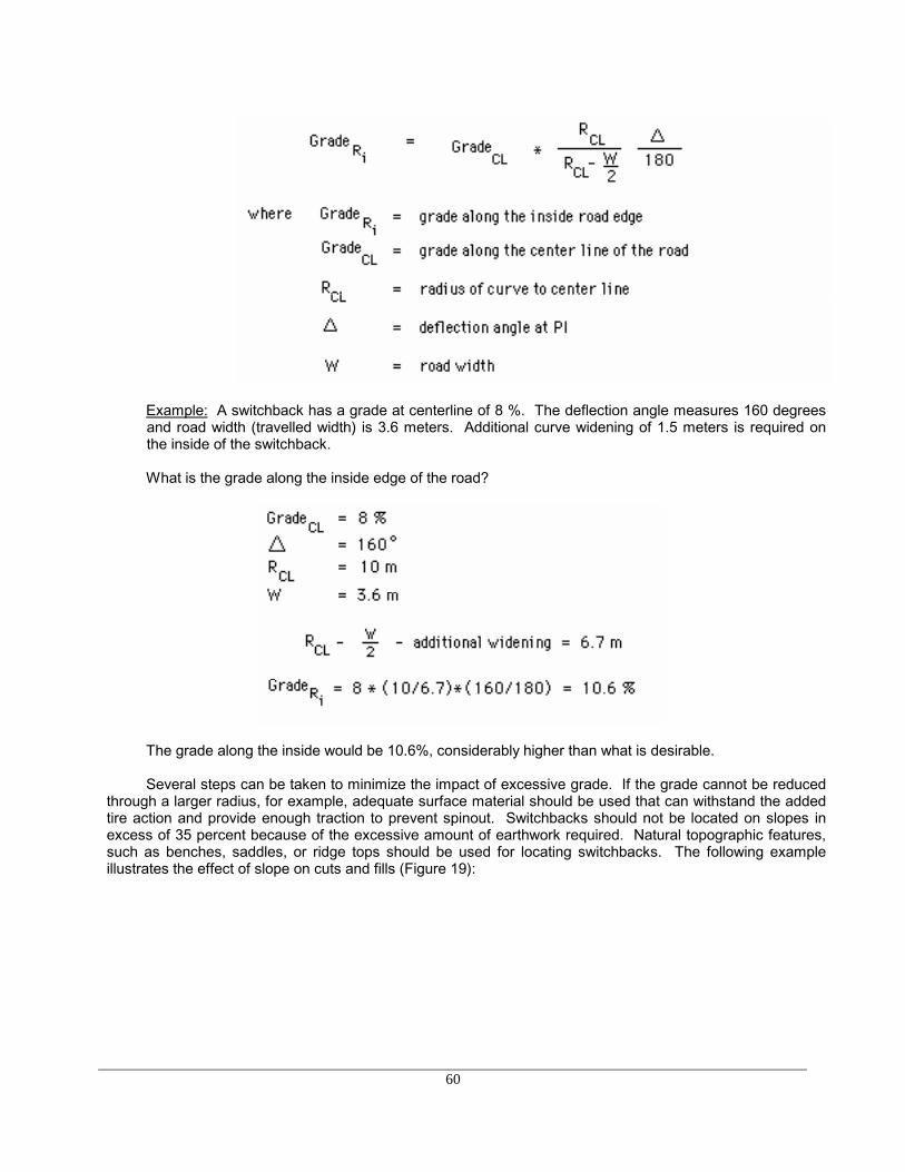
60

Example: A switchback has a grade at centerline of 8 %. The deflection angle measures 160 degreesand road width (travelled width) is 3.6 meters. Additional curve widening of 1.5 meters is required onthe inside of the switchback.

What is the grade along the inside edge of the road?

The grade along the inside would be 10.6%, considerably higher than what is desirable.

Several steps can be taken to minimize the impact of excessive grade. If the grade cannot be reducedthrough a larger radius, for example, adequate surface material should be used that can withstand the addedtire action and provide enough traction to prevent spinout. Switchbacks should not be located on slopes inexcess of 35 percent because of the excessive amount of earthwork required. Natural topographic features,such as benches, saddles, or ridge tops should be used for locating switchbacks. The following exampleillustrates the effect of slope on cuts and fills (Figure 19):

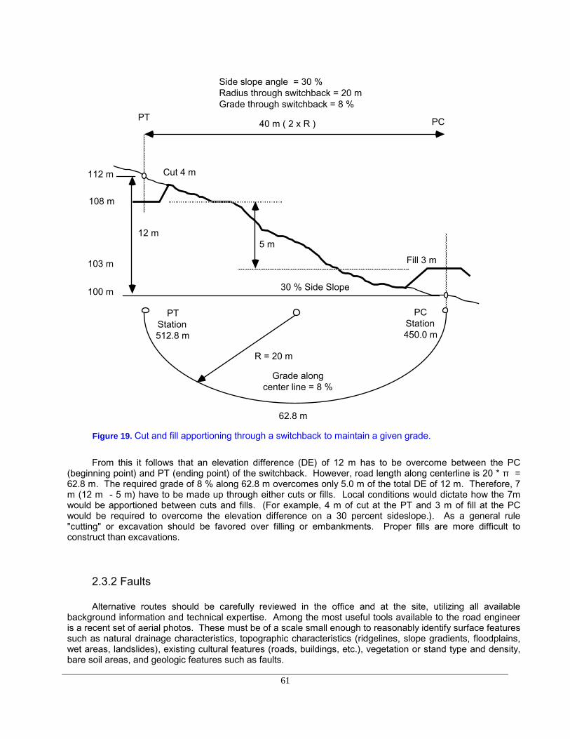
61

112 m

100 m

40 m ( 2 x R )

Cut 4 m

Fill 3 m

108 m

103 m

5 m

PT PC

30 % Side Slope

PT Station 512.8 m

PC Station 450.0 m

R = 20 m

Grade along center line = 8 %

62.8 m

12 m

Side slope angle = 30 % Radius through switchback = 20 m Grade through switchback = 8 %

Figure 19. Cut and fill apportioning through a switchback to maintain a given grade.

From this it follows that an elevation difference (DE) of 12 m has to be overcome between the PC(beginning point) and PT (ending point) of the switchback. However, road length along centerline is 20 * π =62.8 m. The required grade of 8 % along 62.8 m overcomes only 5.0 m of the total DE of 12 m. Therefore, 7m (12 m - 5 m) have to be made up through either cuts or fills. Local conditions would dictate how the 7mwould be apportioned between cuts and fills. (For example, 4 m of cut at the PT and 3 m of fill at the PCwould be required to overcome the elevation difference on a 30 percent sideslope.). As a general rule"cutting" or excavation should be favored over filling or embankments. Proper fills are more difficult toconstruct than excavations.

2.3.2 Faults

Alternative routes should be carefully reviewed in the office and at the site, utilizing all availablebackground information and technical expertise. Among the most useful tools available to the road engineeris a recent set of aerial photos. These must be of a scale small enough to reasonably identify surface featuressuch as natural drainage characteristics, topographic characteristics (ridgelines, slope gradients, floodplains,wet areas, landslides), existing cultural features (roads, buildings, etc.), vegetation or stand type and density,bare soil areas, and geologic features such as faults.

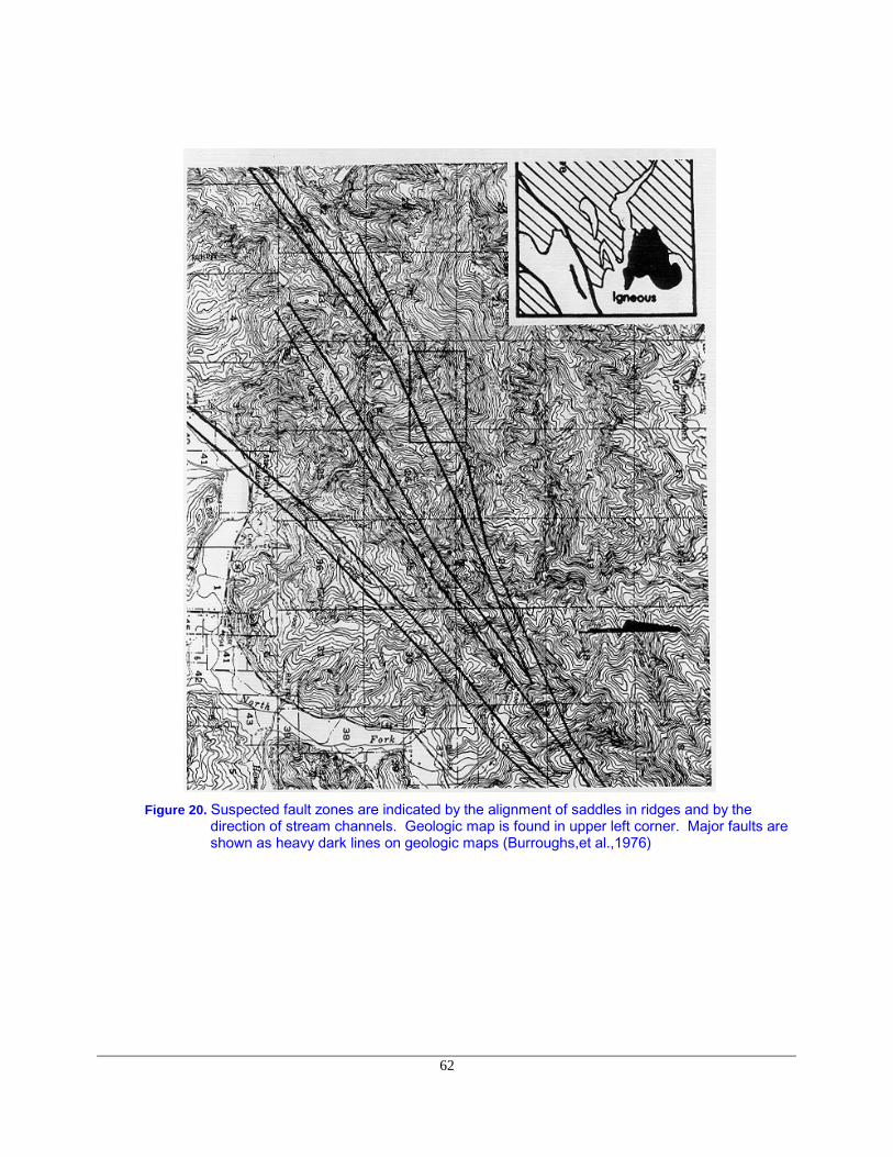
62

Figure 20. Suspected fault zones are indicated by the alignment of saddles in ridges and by thedirection of stream channels. Geologic map is found in upper left corner. Major faults areshown as heavy dark lines on geologic maps (Burroughs,et al.,1976)

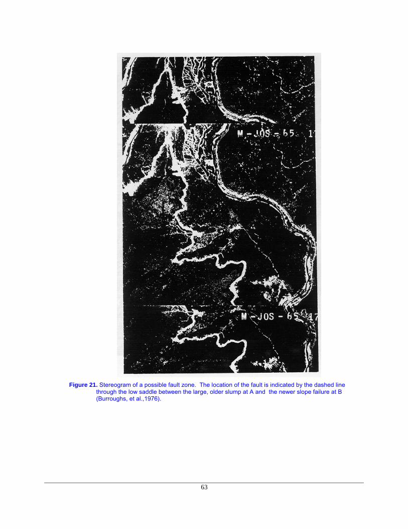
63

Figure 21. Stereogram of a possible fault zone. The location of the fault is indicated by the dashed linethrough the low saddle between the large, older slump at A and the newer slope failure at B(Burroughs, et al.,1976).

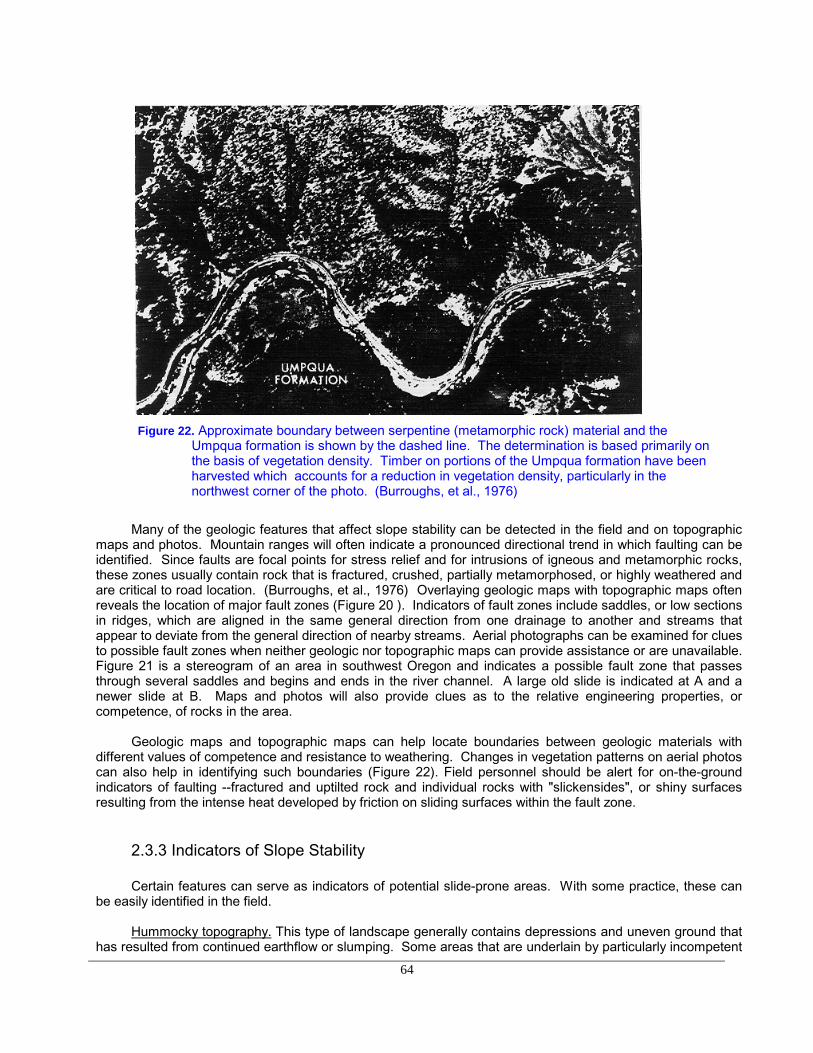
64

Figure 22. Approximate boundary between serpentine (metamorphic rock) material and the

Umpqua formation is shown by the dashed line. The determination is based primarily onthe basis of vegetation density. Timber on portions of the Umpqua formation have beenharvested which accounts for a reduction in vegetation density, particularly in thenorthwest corner of the photo. (Burroughs, et al., 1976)

Many of the geologic features that affect slope stability can be detected in the field and on topographicmaps and photos. Mountain ranges will often indicate a pronounced directional trend in which faulting can beidentified. Since faults are focal points for stress relief and for intrusions of igneous and metamorphic rocks,these zones usually contain rock that is fractured, crushed, partially metamorphosed, or highly weathered andare critical to road location. (Burroughs, et al., 1976) Overlaying geologic maps with topographic maps oftenreveals the location of major fault zones (Figure 20 ). Indicators of fault zones include saddles, or low sectionsin ridges, which are aligned in the same general direction from one drainage to another and streams thatappear to deviate from the general direction of nearby streams. Aerial photographs can be examined for cluesto possible fault zones when neither geologic nor topographic maps can provide assistance or are unavailable.Figure 21 is a stereogram of an area in southwest Oregon and indicates a possible fault zone that passesthrough several saddles and begins and ends in the river channel. A large old slide is indicated at A and anewer slide at B. Maps and photos will also provide clues as to the relative engineering properties, orcompetence, of rocks in the area.

Geologic maps and topographic maps can help locate boundaries between geologic materials withdifferent values of competence and resistance to weathering. Changes in vegetation patterns on aerial photoscan also help in identifying such boundaries (Figure 22). Field personnel should be alert for on-the-groundindicators of faulting --fractured and uptilted rock and individual rocks with "slickensides", or shiny surfacesresulting from the intense heat developed by friction on sliding surfaces within the fault zone.

2.3.3 Indicators of Slope Stability

Certain features can serve as indicators of potential slide-prone areas. With some practice, these canbe easily identified in the field.

Hummocky topography. This type of landscape generally contains depressions and uneven ground thathas resulted from continued earthflow or slumping. Some areas that are underlain by particularly incompetent

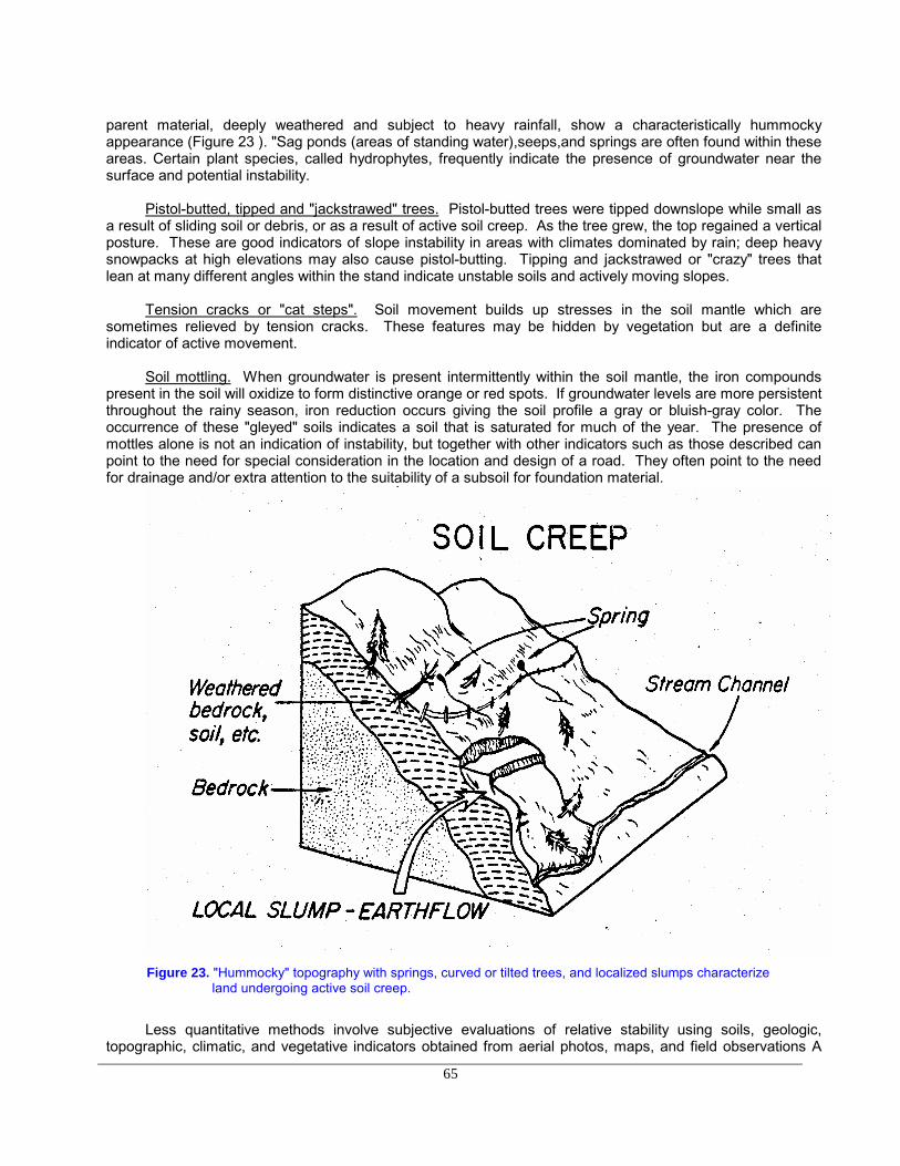
65

parent material, deeply weathered and subject to heavy rainfall, show a characteristically hummockyappearance (Figure 23 ). "Sag ponds (areas of standing water),seeps,and springs are often found within theseareas. Certain plant species, called hydrophytes, frequently indicate the presence of groundwater near thesurface and potential instability.

Pistol-butted, tipped and "jackstrawed" trees. Pistol-butted trees were tipped downslope while small asa result of sliding soil or debris, or as a result of active soil creep. As the tree grew, the top regained a verticalposture. These are good indicators of slope instability in areas with climates dominated by rain; deep heavysnowpacks at high elevations may also cause pistol-butting. Tipping and jackstrawed or "crazy" trees thatlean at many different angles within the stand indicate unstable soils and actively moving slopes.

Tension cracks or "cat steps". Soil movement builds up stresses in the soil mantle which aresometimes relieved by tension cracks. These features may be hidden by vegetation but are a definiteindicator of active movement.

Soil mottling. When groundwater is present intermittently within the soil mantle, the iron compoundspresent in the soil will oxidize to form distinctive orange or red spots. If groundwater levels are more persistentthroughout the rainy season, iron reduction occurs giving the soil profile a gray or bluish-gray color. Theoccurrence of these "gleyed" soils indicates a soil that is saturated for much of the year. The presence ofmottles alone is not an indication of instability, but together with other indicators such as those described canpoint to the need for special consideration in the location and design of a road. They often point to the needfor drainage and/or extra attention to the suitability of a subsoil for foundation material.

Figure 23. "Hummocky" topography with springs, curved or tilted trees, and localized slumps characterizeland undergoing active soil creep.

Less quantitative methods involve subjective evaluations of relative stability using soils, geologic,topographic, climatic, and vegetative indicators obtained from aerial photos, maps, and field observations A

66

headwall rating system such as the one presented in Figure 24 can be used to broadly evaluate relativestability of a particular site. The rating obtained in the field is entered into an empirical slope stability model toevaluate various timber harvesting options. As with most subjective rating systems, consistency among fieldpersonnel is a major problem. However, they accurately represent the relative importance of individualfactors and their effects on likelihood of failure by mass movement type. The weighted values for hazardindices are presented as guides only, and can be adjusted to reflect local conditions.

67

Figure 24. Empirical headwall rating system.used for shallow, rapid landslides on the Mapleton RangerDistrict, U.S. Forest Service, Region 6, Oregon.

68

LITERATURE CITED

Bishop, D. M. and M. E. Stevens. 1964. Landslides on logged areas in southeast Alaska. USDA ForestService Research Paper PNW-1, 18 pp.

Burroughs, E. R. and J. G. King. 1985. Surface erosion control on roads in granitic soils. Inland EmpireForest Engineering Conference. Moscow, Idaho. February, 1985. 8 pp.

Burroughs, E. R. Jr., G. R. Chalfant, and M. A. Townsend. 1976. Slope stability in road construction. U. S.Department of the Interior. Bureau of Land Management, Oregon State Office.102 pp.

Dietz, P., W. Knigge and H. Loeffler. 1984. Walderschliessung. Verlag Paul Parey, Hamburg and Berlin,Germany.

Gardner, R. B. 1978. Cost, performance, and esthetic impacts of an experimental forest road in Montana.USDA Forest Service Research Paper INT-203. 28 pp.

Gardner, R. B. 1971. Forest road standards as related to economics and the environment. USDA ForestService Research Note INT-45. 4 pp.

Hickerson, T. F. 1964. Route location and design. Fifth Ed. McGraw-Hill Co., New York. 634 pp.

Kuonen, V. 1983. Wald-und Gueterstrassen. Eigenverlag, V. Kuonen, Lindenweg 9, CH-8122. Pfaffhausen,Switzerland.

Pearce, J. K. 1960. Forest Engineering Handbook. Prepared for US Dept. of the Interior, Bureau of LandManagement. 220 pp.

Rice, R. M. 1977. Forest management to minimize landslide risk. In "Guidelines for WatershedManagement". Food and Agriculture Organization of the United Nations, Rome, 1977. pp. 271-287.

Segebaden von, G., 1964. Studies of cross-country transport distances and road net extension. StudiaForestalia Suedica, No. 18.

Sidle, R. C. 1980. Slope stability on forest land. USDA Forest Service Research Paper PNW-209. 23 pp.

Transportation Research Board, 1978. Geometric design standards for low-volume roads, Com- pendium 1.National Academy of Sciences and U.S. Agency for International Development, Washington, D.C.

U. S. Department of Agriculture, Forest Service. 1960. Logging Road Handbook. Agricultural Handbook No.

183. 65 pp.

U. S. Department of Agriculture, Forest Service. 1982. Transportation Engineering Handbook

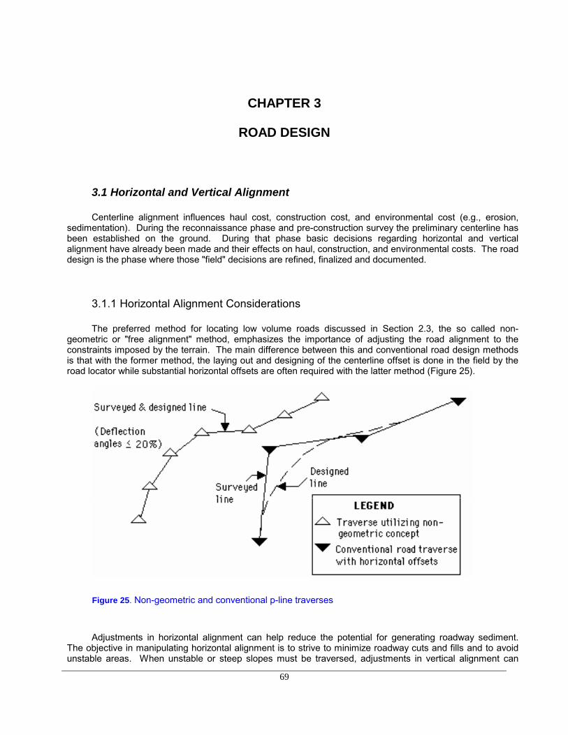
69

CHAPTER 3

ROAD DESIGN

3.1 Horizontal and Vertical Alignment

Centerline alignment influences haul cost, construction cost, and environmental cost (e.g., erosion,sedimentation). During the reconnaissance phase and pre-construction survey the preliminary centerline hasbeen established on the ground. During that phase basic decisions regarding horizontal and verticalalignment have already been made and their effects on haul, construction, and environmental costs. The roaddesign is the phase where those "field" decisions are refined, finalized and documented.

3.1.1 Horizontal Alignment Considerations

The preferred method for locating low volume roads discussed in Section 2.3, the so called non-geometric or "free alignment" method, emphasizes the importance of adjusting the road alignment to theconstraints imposed by the terrain. The main difference between this and conventional road design methodsis that with the former method, the laying out and designing of the centerline offset is done in the field by theroad locator while substantial horizontal offsets are often required with the latter method (Figure 25).

Figure 25. Non-geometric and conventional p-line traverses

Adjustments in horizontal alignment can help reduce the potential for generating roadway sediment.The objective in manipulating horizontal alignment is to strive to minimize roadway cuts and fills and to avoidunstable areas. When unstable or steep slopes must be traversed, adjustments in vertical alignment can

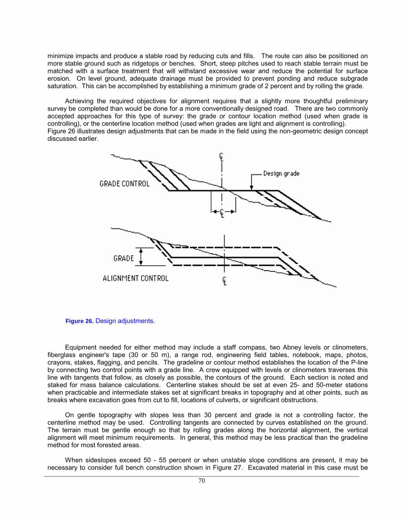
70

minimize impacts and produce a stable road by reducing cuts and fills. The route can also be positioned onmore stable ground such as ridgetops or benches. Short, steep pitches used to reach stable terrain must bematched with a surface treatment that will withstand excessive wear and reduce the potential for surfaceerosion. On level ground, adequate drainage must be provided to prevent ponding and reduce subgradesaturation. This can be accomplished by establishing a minimum grade of 2 percent and by rolling the grade.

Achieving the required objectives for alignment requires that a slightly more thoughtful preliminarysurvey be completed than would be done for a more conventionally designed road. There are two commonlyaccepted approaches for this type of survey: the grade or contour location method (used when grade iscontrolling), or the centerline location method (used when grades are light and alignment is controlling).Figure 26 illustrates design adjustments that can be made in the field using the non-geometric design conceptdiscussed earlier.

Figure 26. Design adjustments.

Equipment needed for either method may include a staff compass, two Abney levels or clinometers,fiberglass engineer's tape (30 or 50 m), a range rod, engineering field tables, notebook, maps, photos,crayons, stakes, flagging, and pencils. The gradeline or contour method establishes the location of the P-lineby connecting two control points with a grade line. A crew equipped with levels or clinometers traverses thisline with tangents that follow, as closely as possible, the contours of the ground. Each section is noted andstaked for mass balance calculations. Centerline stakes should be set at even 25- and 50-meter stationswhen practicable and intermediate stakes set at significant breaks in topography and at other points, such asbreaks where excavation goes from cut to fill, locations of culverts, or significant obstructions.

On gentle topography with slopes less than 30 percent and grade is not a controlling factor, thecenterline method may be used. Controlling tangents are connected by curves established on the ground.The terrain must be gentle enough so that by rolling grades along the horizontal alignment, the verticalalignment will meet minimum requirements. In general, this method may be less practical than the gradelinemethod for most forested areas.

When sideslopes exceed 50 - 55 percent or when unstable slope conditions are present, it may benecessary to consider full bench construction shown in Figure 27. Excavated material in this case must be

71

end hauled to a safe location. Normally, the goal of the road engineer is to balance earthwork so that thevolume of fill equals the volume of cut plus any gain from bulking less any loss from shrinkage (Figure 28).

Road design, through its elements such as template (width, full bench/side cast), curve widening andgrade affect the potential for erosion. Erosion rates are directly proportional to the total exposed area in cutsand fills. Road cuts and fills tend to increase with smooth, horizontal and vertical alignment. Conversely,short vertical and horizontal tangents tend to reduce cuts and fills. Erosion rates can be expected to be lowerin the latter case. Prior to the design phase it.

Figure 27. Full bench design.

Figure 28. Self-balanced design

72

should be clearly stated which alignment, horizontal or vertical, takes precedence. For example, if thetag line has been located at or near the permissible maximum grade, the vertical alignment will govern. Truckspeeds in this case are governed by grade and not curvature. Therefore, horizontal alignment of thecenterline can follow the topography very closely in order to minimize earthwork. Self balancing sectionswould be achieved by shifting the template horizontally.

3.1.2 Curve Widening

Roadway safety will be in jeopardy and the road shoulders will be impacted by off-tracking wheels ifvehicle geometry and necessary curve widening are not considered properly. Continually eroding shoulderswill become sedimentation source areas and will eventually weaken the road. On the other hand, over designwill result in costly excessive cuts and/or fills.

The main principle of off-tracking and hence curve widening, centers on the principle that all vehicleaxles rotate about a common center. Minimum curve radius is vehicle dependent and is a function ofmaximum cramp angle and wheelbase length (see Figure 29).

R1 = Radius to outside front wheel R2 = Radius to inside rear wheel R3 = Radius to center front axle = minimum curve radius a = cramp angle of steering wheel MRW= Minimum road width (R1 - R2 ); add 0.5 to 0.7 m for driver error and safety.

R1

R2

COR

L1

a

a

R3

MRW

R3 = L1 / SIN (a)

Figure 29. Basic vehicle geometry in off-tracking

Typical vehicle dimensions are shown in Figure 30 for single trucks, truck/ trailers, log truck (pole-type),and tractor/trailer combinations. These dimensions were used to develop Figures 35 to 38 for calculatingcurve widening in relation to curve radius and central angle.

73

Several different solutions to determine curve widening requirements are in use. Most mathematicalsolutions and their simplified versions give the maximum curve widening required. Curve widening is afunction of vehicle dimensions, curve radius, and curve length (central angle).

A graphical solution to the problem is provided in Figures 31 to 33. This solution can be used for singletrucks, truck-trailer combinations and vehicle overhang situations. This solution provides the maximum curvewidening for a given curve radius.

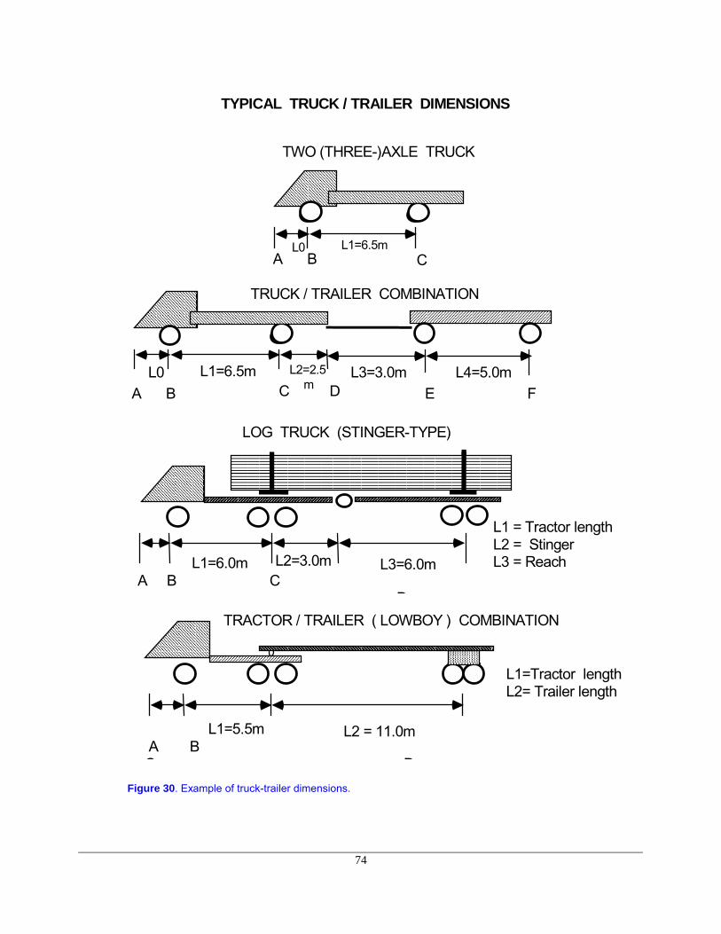
74

A B C DL2=2.5

mL0 L3=3.0m L4=5.0m

E F

TRUCK / TRAILER COMBINATION

L1=6.0m L2=3.0m L3=6.0m

L1 = Tractor lengthL2 = StingerL3 = Reach

LOG TRUCK (STINGER-TYPE)

L1=5.5m L2 = 11.0m

TRACTOR / TRAILER ( LOWBOY ) COMBINATION

L1=Tractor lengthL2= Trailer length

TYPICAL TRUCK / TRAILER DIMENSIONS

A B CD

A BC D

A B CL0

TWO (THREE-)AXLE TRUCK

L1=6.5m

L1=6.5m

Figure 30. Example of truck-trailer dimensions.

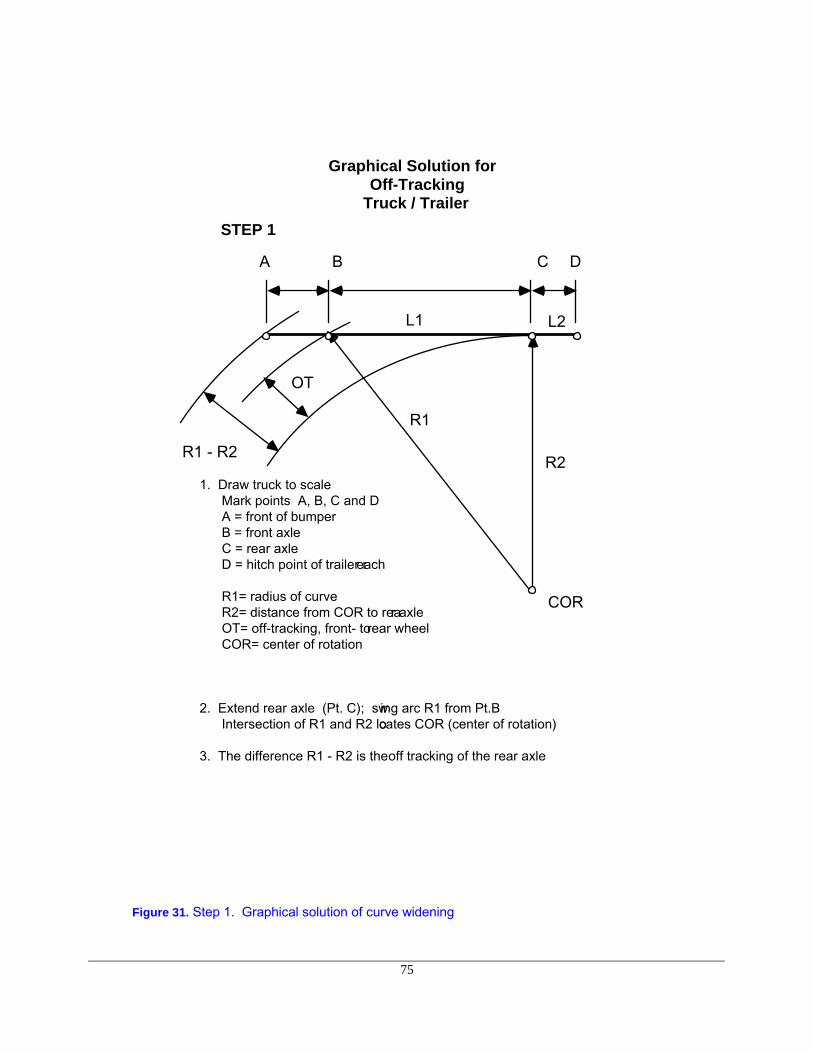
75

R1

R2

OT

COR

A B C D

L2

1. Draw truck to scale Mark points A, B, C and D A = front of bumper B = front axle C = rear axle D = hitch point of trailer reach R1= radius of curve R2= distance from COR to rear axle OT= off-tracking, front- to rear wheel COR= center of rotation 2. Extend rear axle (Pt. C); swing arc R1 from Pt.B Intersection of R1 and R2 locates COR (center of rotation) 3. The difference R1 - R2 is the off tracking of the rear axle

L1

Graphical Solution for

Off-Tracking Truck / Trailer

R1 - R2

STEP 1

Figure 31. Step 1. Graphical solution of curve widening

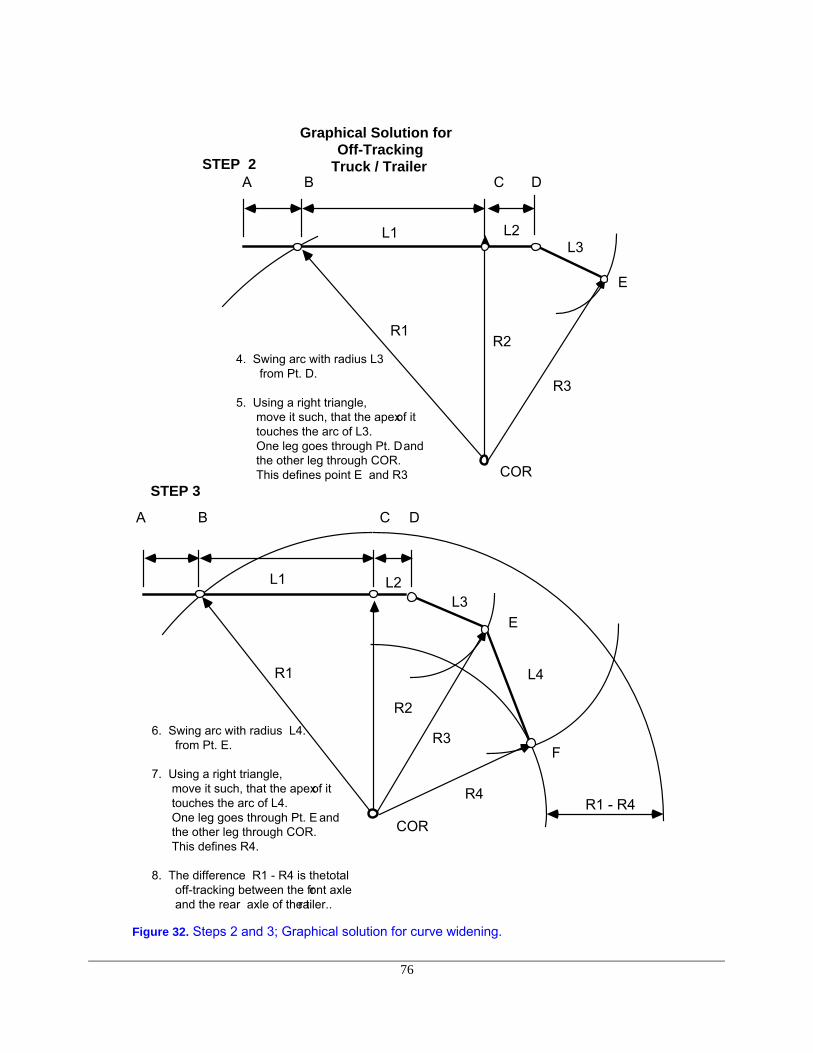
76

Graphical Solution for

Off-Tracking Truck / Trailer

COR

STEP 2

R1R2

A B C D

L2L1

R3

4. Swing arc with radius L3 from Pt. D. 5. Using a right triangle, move it such, that the apex of it touches the arc of L3. One leg goes through Pt. D and the other leg through COR. This defines point E and R3

L3

STEP 3

R1

R2

COR

L2L1

R36. Swing arc with radius L4. from Pt. E. 7. Using a right triangle, move it such, that the apex of it touches the arc of L4. One leg goes through Pt. E and the other leg through COR. This defines R4. 8. The difference R1 - R4 is the total off-tracking between the front axle and the rear axle of the trailer..

L3

R4

L4

E

F

R1 - R4

A B C D

E

Figure 32. Steps 2 and 3; Graphical solution for curve widening.

77

The graphical solution for a stinger type log truck is shown in Figure 33. Here, an arc with the bunklength L2 plus L3 is drawn with the center at C. The log load swivels on the bunks, C and E and forms line C -E, with the trailer reach forming line D - E.

COR

R1

L1 L2

R2

L3

R3

R1 - R3

GRAPHICAL SOLUTION STINGER-TYPE LOG TRUCK

R1 - R3 is the total off-tracking between front- and rear axle

of trailer

B C D

E

Points C and E are the log bunks. Point D is the connector between stinger and reach.

R3

Figure 33. Graphical solution for off-tracking of a stinger-type log truck

Simple, empirical curve widening formulae have been proposed by numerous authors and governmentagencies. A common method used in North America is:

CW = 37/R For Tractor-trailer (low boy; units in meters)

CW =18.6/R For log-truck (units in meters)

The above equations are adapted for the typical truck dimensions used in the United States andCanada. In Europe, curve widening recommendations vary from 14/R to 32/R. Curve wideningrecommendations in Europe are given by Kuonen (1983) and Dietz et al. (1984). Kuonen defines the curvewidening requirement for a two-axle truck (wheelbase = 5.5m) as

CW = 14/R

and a truck-trailer combination where

CW = 26/R

78

Dietz, et. al. (1984) recommend CW=32/R for any truck combination.

The approximation methods mentioned above are usually not satisfactory under difficult or critical terrainconditions. They typically overestimate curve widening requirements for wide curves (central angle < 45o )and under estimate them for tight curves (central angle > 50o ).

Vehicle tracking simulation provides a better vehicle off-tracking solution because it considers vehiclegeometry and curve elements, in particular the deflection angle (Kramer, 1982, Cain & Langdon, 1982). Thefollowing charts provide off-tracking for four common vehicle configurations--a single or two-axle truck, atruck-trailer combination, a stinger-type log-truck and a tractor-trailer (lowboy) combination. The charts arevalid for the specified vehicle dimensions and are based on the following equation (Cain and Langdon, 1982):

OF = (R - (R2 - L2) 1/2) * (1 - eX)

where x =( -0.015 * D * R/L + 0.216)OF = Off tracking (m)R = Curve radius (m)D = Deflection angle or central anglee = Base for natural logarithm (2.7183)L = Total combination wheelbase of vehicleL = (Summation of Li2)1/2

For a log-truck:

L= (L12 + L22 + L32)1/2

where L1-3 are defined in Figure 30.

The maximum off-tracking for a given vehicle, radius and deflection angle occurs when the vehicleleaves the curve. Since vehicles travel both directions, the required curve widening, which consists of off-tracking (OT) plus safety margin (0.5 - 0.6m), should be added to the full curve length. One half of therequired curve widening should be added to the inside and one half to the outside of the curve (Figure 34).

79

9 - 18 m9 - 18 m

Taper length

1/2 CW

1/2 CW

Figure 34. Curve widening and taper lengths.

Figures 35 through 38 provide vehicle off-tracking for a given vehicle, radius, and deflection (or centralangle). To this value, 0.5 to 0.6m should be added to allow for formula and driver's error, grade, and road orsuper elevation variations.

Transition or taper length from tangent to curve vary from 9 to 18 m depending on curve radius.Recommended length of transition before and after a curve are as follows (Cain and Langdon, 1982):

Curve Radius (m) Length of Taper (m)

20 1820 - 25 1525 - 30 12

30 10

Example: Standard road width is 3.0 m. Design vehicle is a stinger-type log-truck with dimensions asshown in Figure 30. Curve radius is 22m, deflection angle equals 60o.

From Figure 37 locate curve radius on the x-axis (interpolate between 20 and 25), go up to thecorresponding 60o- curve (interpolate between 45o and 90o), go horizontally to the left and read thevehicle off-tracking equal to 1.8 m.

The total road width is 4.80 m ( 3.0 m + 1.8 m ).

Depending on conditions, a safety margin of 0.5 m could be added. The current 3.0 m road widthalready allows for safety and driver's error of 0.30 m on either side of the vehicle wheels (truck width = 2.40

80

m). Depending on the ballast depth, some additional shoulder width may be available for driver's error. Taperlength would be 15 m.

0

0.5

1

1.5

2

2.5

10 15 20 25 30 40

<20

30

45

90

>180

CURVE WIDENING FORTWO-AXLE TRUCK

6.5 m.

CURVE RADIUS (METERS)

CENTRAL ANGLE(DEGREES)

CURVE WIDENING(METERS)

L1=6.5m

Figure 35. Curve widening guide for a two or three axle truck as a function of radius and deflectionangle. The truck dimensions are as shown.

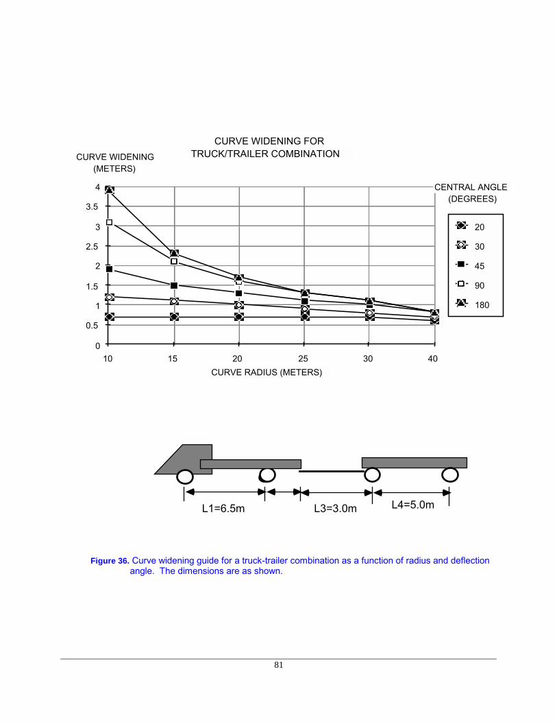
81

0

0.5

1

1.5

2

2.5

3

3.5

4

10 15 20 25 30 40

20

30

45

90

180

CURVE WIDENING FORTRUCK/TRAILER COMBINATION

CURVE RADIUS (METERS)

CURVE WIDENING(METERS)

CENTRAL ANGLE(DEGREES)

L1=6.5m L3=3.0m L4=5.0m

Figure 36. Curve widening guide for a truck-trailer combination as a function of radius and deflectionangle. The dimensions are as shown.

82

0

1

2

3

4

5

6

10 15 20 25 30 40

<20

30

45

90

>180

CURVE WIDENING FORLOG-TRUCK (POLE TRAILER)

CURVE RADIUS (METERS)

CENTRAL ANGLE(DEGREES)

CURVE WIDENING(METERS)

L1=6.0m L2=3.0m L3=6.0m

Figure 37. Curve widening guide for a log-truck as a function of radius and deflection angle. Thedimensions are as shown.

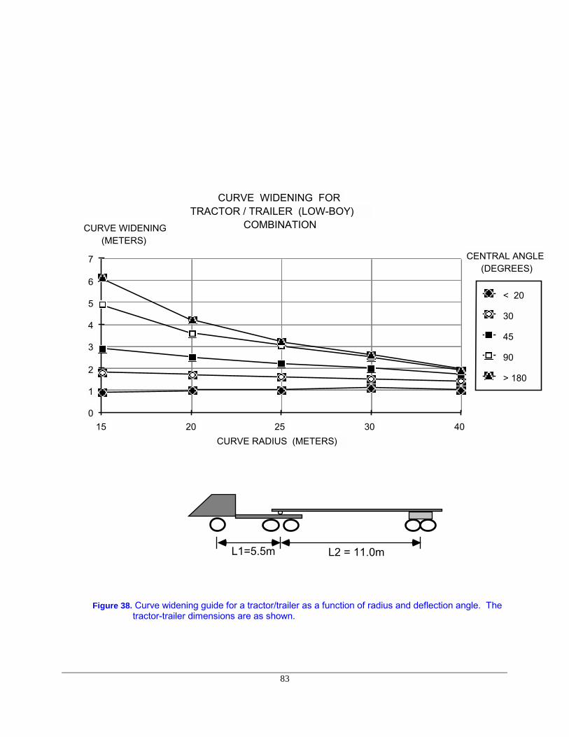
83

0

1

2

3

4

5

6

7

15 20 25 30 40

< 20

30

45

90

> 180

CURVE WIDENING FORTRACTOR / TRAILER (LOW-BOY)

COMBINATION

CURVE RADIUS (METERS)

CURVE WIDENING(METERS)

CENTRAL ANGLE(DEGREES)

L1=5.5m L2 = 11.0m

Figure 38. Curve widening guide for a tractor/trailer as a function of radius and deflection angle. Thetractor-trailer dimensions are as shown.

84

3.1.3 Vertical Alignment

Vertical alignment is often the limiting factor in road design for most forest roads. Frequently grades ortag lines are run at or near the maximum permissible grade. Maximum grades are determined by eithervehicle configuration (design/critical vehicle characteristic) or erosive conditions such as soil or precipitationpatterns. Depending on road surface type, a typical logging truck can negotiate different grades. Table 16lists maximum grades a log truck can start from. It should be noted that today's loaded trucks are tractionlimited and not power limited. They can start on grades up to 25 % on dry, well maintained, unpaved roads.Once in motion they can typically negotiate steeper grades.

Vertical curves or grade changes, like horizontal curves, require proper consideration to minimizeearthwork, cost, and erosion damage. Proper evaluation requires an analysis of vertical curve requirementsbased on traffic characteristics (flow and safety), vehicle geometry, and algebraic difference of intersectinggrades.

Vertical curves provide the transition between an incoming grade and an outgoing grade. Forconvenience in design, a parabolic curve (Figures 39 and 40) is used because the grade change isproportional to the horizontal distance. The grade change is the difference between incoming grade andoutgoing grade. The shorter the vertical curve can be kept, the smaller the earthwork required.

VPI

CONVEX CREST CURVE

VPI

CONCAVE SAG CURVE

Figure 39. Typical vertical curves( VPI = Vertical Point of Intersection).

The grade change per unit length is defined as

(G1 -G2) / L (% / meter)

or more commonly its inverse, where the grade change is expressed in horizontal distance (meters) toeffect a 1% change in grade.

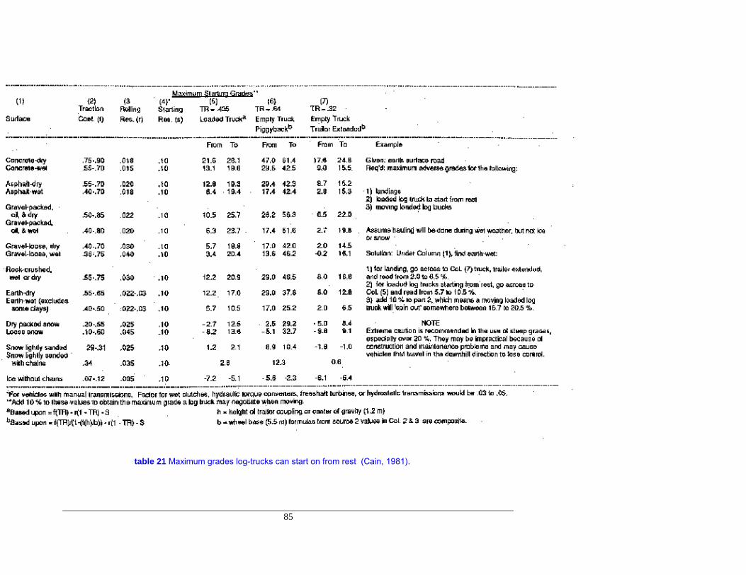
85

table 21 Maximum grades log-trucks can start on from rest (Cain, 1981).

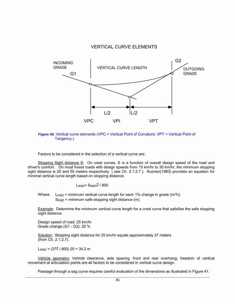
86

VPC VPI VPT

OUTGOING GRADE

L/2 L/2

G1

G2VERTICAL CURVE LENGTH

INCOMING GRADE

VERTICAL CURVE ELEMENTS

Figure 40. Vertical curve elements (VPC = Vertical Point of Curvature; VPT = Vertical Point ofTangency ).

Factors to be considered in the selection of a vertical curve are:

Stopping Sight distance S: On crest curves, S is a function of overall design speed of the road anddriver's comfort. On most forest roads with design speeds from 15 km/hr to 30 km/hr, the minimum stoppingsight distance is 20 and 55 meters respectively ( see Ch. 2.1.2.7 ). Kuonen(1983) provides an equation forminimal vertical curve length based on stopping distance:

Lmin= Smin2 / 800

Where Lmin = minimum vertical curve length for each 1% change in grade (m/%)Smin = minimum safe stopping sight distance (m).

Example: Determine the minimum vertical curve length for a crest curve that satisfies the safe stoppingsight distance.

Design speed of road: 25 km/hrGrade change (G1 - G2): 20 %

Solution: Stopping sight distance for 25 km/hr equals approximately 37 meters(from Ch. 2.1.2.7).

Lmin = (372 / 800) 20 = 34.2 m

Vehicle geometry: Vehicle clearance, axle spacing, front and rear overhang, freedom of verticalmovement at articulation points are all factors to be considered in vertical curve design.

Passage through a sag curve requires careful evaluation of the dimensions as illustrated in Figure 41.

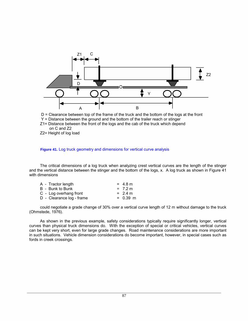
87

D

Z1

Z2

Y

C

A B D = Clearance between top of the frame of the truck and the bottom of the logs at the front Y = Distance between the ground and the bottom of the trailer reach or stingerZ1= Distance between the front of the logs and the cab of the truck which depend

on C and Z2Z2= Height of log load

Figure 41. Log truck geometry and dimensions for vertical curve analysis

The critical dimensions of a log truck when analyzing crest vertical curves are the length of the stingerand the vertical distance between the stinger and the bottom of the logs, x. A log truck as shown in Figure 41with dimensions

A - Tractor length = 4.8 mB - Bunk to Bunk = 7.2 mC - Log overhang front = 2.4 mD - Clearance log - frame = 0.39 m

could negotiate a grade change of 30% over a vertical curve length of 12 m without damage to the truck(Ohmstede, 1976).

As shown in the previous example, safety considerations typically require significantly longer, verticalcurves than physical truck dimensions do. With the exception of special or critical vehicles, vertical curvescan be kept very short, even for large grade changes. Road maintenance considerations are more importantin such situations. Vehicle dimension considerations do become important, however, in special cases such asfords in creek crossings.

88

3.2 Road Prism

Proper design of the roadway prism can significantly reduce the amount of sediment and debris thatenters adjacent streams. Often the basic cause of a particular mass failure can be traced to overroading oroverdesign. Overroading or misplacement of roads results from a poor land management or transportationplan; overdesign results from rigidly following design criteria with respect to curvature, width, gradient, andoversteepened cuts and fills or from designing roads to higher standards than are required for their intendeduse. As stated previously, allowing terrain characteristics to govern road design permits more flexibility andwill be especially beneficial, both environmentally and economically, where it is possible to reduce cut and fillslope heights, slope angles, and roadway widths.

3.2.1 Road Prism Stability

Stability considerations as applied to natural slopes are also valid for stability analysis of road cuts andfills. Points to consider include

- Critical height of cut slope or fill slope- Critical piezometric level in a slope or road fill- Critical cut slope and fill slope angle.

The most common road fill or sidecast failure mode is a translational slope failure. Translational slopefailure is characterized by a planar failure surface parallel to the ground or slope. Depth to length ratio ofslides are typically very small. The following slopes would fall into this category:

1. Thin, residual soil overlaying an inclined bedrock contact2. Bedrock slopes covered with glacial till or colluvium3. Homogeneous slopes of coarse textured, cohesionless soils (road fills)

Fill slope failure can occur in two typical modes. Shallow sloughing at the outside margins of a fill is anexample of limited slope failure which contributes significantly to erosion and sedimentation but does notdirectly threaten the road. It is usually the result of inadequate surface protection. The other is sliding of theentire fill along a contact plane which can be the original slope surface or may include some additional soillayers. It results from lack of proper fill compaction and/or building on too steep a side slope. Another reasoncould be a weak soil layer which fails under the additional weight placed on it by the fill.

Slope or fill failure is caused when forces causing or promoting failure exceed forces resisting failure(cohesion, friction, etc.). The risk of failure is expressed through the factor of safety (see Figure 2):

FS = Shear strength/ Shear stress

where shear strength is defined as

T = C * A +N (tan [f])

and shear stress, the force acting along the slope surface, is defined as

D = W * sin[b]

89

where C = Cohesive strength (tonnes/m2) A = Contact area (m2) W = Unit weight of soil (tonne/m3)[b] = Ground slope angle[f] = Coefficient of friction or friction angle (Table 17) N = Normal force = W * cos[b].

table 23 Values of friction angles and unit weights for various soils. (from Burroughs, et. al., 1976)

---------------------------------------------------------------------------------------------------------------------Soil type Density Friction Angle Unit Soil Weight

Degrees Tonnes/m3---------------------------------------------------------------------------------------------------------------------

Coarse Sand Compact 45 2.24Gravel Firm 38 1.92

Loose 32 1.44

Medium Sand Compact 40 2.08 Firm 34 1.76

Loose 30 1.44

Fine Silty Compact 32 2.08 sands Firm 30 1.60

Loose 28 1.36

Uniform Silts Compact 30 1.76Loose 26 1.36

Clay- Silt Medium 15 - 20 1.92Soft 15 - 20 1.44

Clay Medium 0 - 10 1.92Soft 0 - 10 1.44

---------------------------------------------------------------------------------------------------------------------

The friction angle is also referred to as the angle of repose. Sand or gravel cannot be used to form asteeper slope than the frictional angle allows. In other words, the maximum fill angle of a soil cannot exceedits coefficient of friction. Typical friction angles are given in Table 17. One should note the change in soilstrength from "loose" to "compact" indicating the improvement in cohesion brought about by proper soilcompaction.

Cohesionless soils such as sands or gravel without fines (clay) derive their strength from frictionalresistance only

T = W * cos[b] * tan[f]

while pure clays derive their shear strength from cohesion or stickiness. Shear strength or cohesive strengthof clay decreases with increasing moisture making clays very moisture sensitive.

The factor of safety against sliding or failure can be expressed as:

FS = {C * A + (W * cos[b] * tan [f] ) } / { W * sin[b] }

90

In cases where the cohesive strength approaches zero (granular soils, high moisture content) the factorof safety simplifies to

FS = tan[f] / tan[b] (C= 0)

Road fills are usually built under dry conditions. Soil strength, particularly, cohesive strength is highunder such conditions. If not planned or controlled, side cast fills are often built at the maximum slope anglethe fill slope will stand (angle of repose). The fill slope, hence, has a factor of safety of one or just slightlylarger than one. Any change in conditions, such as added weight on the fill or moisture increase, will lower thefactor of safety, and the fill slope will fail. It is clear that the factor of safety must be calculated from "worstcase" conditions and not from conditions present at the time of construction.

Failure can be brought about in one of two ways:

1. Translational fill failure (Figure 42) can be brought about by a build-up of a saturated zone. Frictionalstrength or grain-to-grain contact is reduced by a bouyancy force. Rainfall and/or ponded ditch waterseeping into the fill are often responsible for this type of failure.

Y

L

A1 - Wet Fill Area

A2 - Saturated Zone

Hw - Depth of saturated zone L - Length of fill b - slope angle

A2 = ( L ) x (Hw) x (cos (b)) b

RAIN

DITCH OVERFLOW

Hw

TRANSLATIONAL FAILURE

Figure 42. Translational or wedge failure brought about by saturated zone in fill. Ditch overflow orunprotected surfaces are often responsible.

The factor of safety against a translational failure can be shown to be:

FS ={ [ C* A1 + g buoy * A2] * tan[f] } / { [ g*A1 + gsat * A2] * tan[b] }

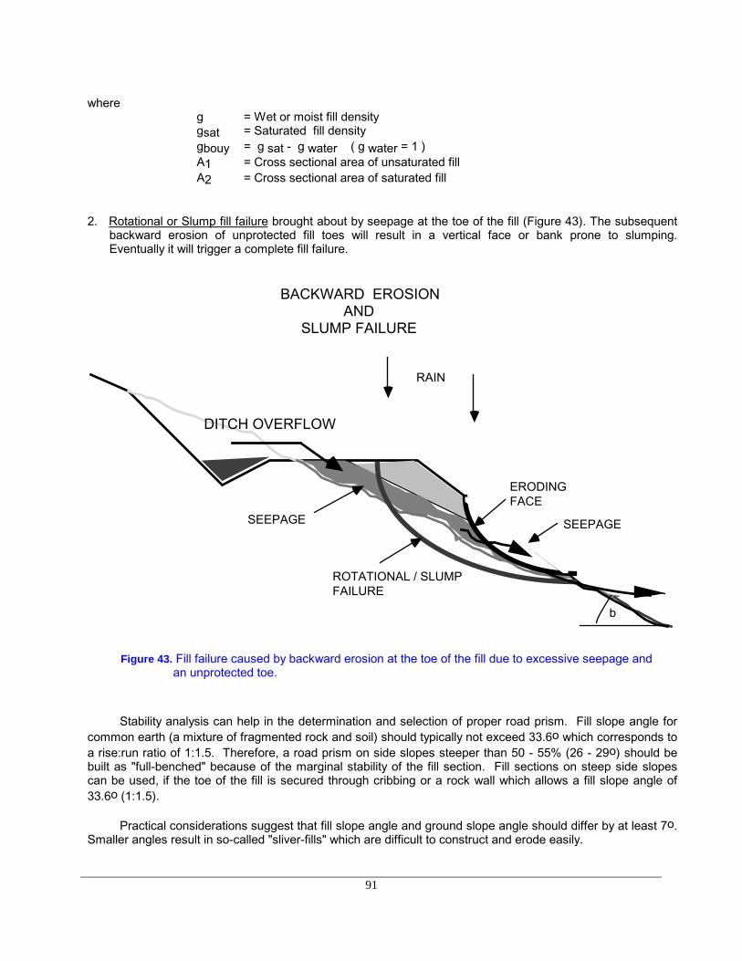
91

whereg = Wet or moist fill densitygsat = Saturated fill densitygbouy = g sat - g water ( g water = 1 )A1 = Cross sectional area of unsaturated fillA2 = Cross sectional area of saturated fill

2. Rotational or Slump fill failure brought about by seepage at the toe of the fill (Figure 43). The subsequentbackward erosion of unprotected fill toes will result in a vertical face or bank prone to slumping.Eventually it will trigger a complete fill failure.

DITCH OVERFLOW

b

SEEPAGE

ROTATIONAL / SLUMP FAILURE

ERODING FACE

BACKWARD EROSION AND

SLUMP FAILURE

RAIN

SEEPAGE

Figure 43. Fill failure caused by backward erosion at the toe of the fill due to excessive seepage andan unprotected toe.

Stability analysis can help in the determination and selection of proper road prism. Fill slope angle forcommon earth (a mixture of fragmented rock and soil) should typically not exceed 33.6o which corresponds toa rise:run ratio of 1:1.5. Therefore, a road prism on side slopes steeper than 50 - 55% (26 - 29o) should bebuilt as "full-benched" because of the marginal stability of the fill section. Fill sections on steep side slopescan be used, if the toe of the fill is secured through cribbing or a rock wall which allows a fill slope angle of33.6o (1:1.5).

Practical considerations suggest that fill slope angle and ground slope angle should differ by at least 7o.Smaller angles result in so-called "sliver-fills" which are difficult to construct and erode easily.

92

Example: Ground slope = 50%Fill slope = 66.7%

Assuming zero cohesion and friction angle equals fill angle ([f] = [b])

FS = tan[f] / tan[b] = 0.667 / 0.50 = 1.33

The factor of safety is adequate. The fill slope stability becomes marginal if the same road prism (fillslope angle = 33.7o) is built on a 60% side slope. The factor of safety becomes

FS = 0.667/0.600 = 1.11

The factor of safety in this case would be considered marginal. Here the difference between fill slopeangle and ground slope is less than 7o, a sliver fill.

Cut slope failures in road construction typically occur as a rotational failure. It is common in these casesto assume a circular slip surface. Rotational failures can be analyzed by the method of slices, probably themost common method for analyzing this type of failure (Bishop,1950; Burroughs, et. al.,1976).

Numerous stability charts have been developed for determining the critical height of a cut for a specificsoil characterized by cohesion, friction angle, and soil density. The critical height, Hcrit, is the maximumheight at which a slope will remain stable. They are related to a stability number, Ns, defined as

Ns = Hcrit (C/[g]).

Chen and Giger (1971) and Prellwitz (1975) published slope stability charts for the design of cut and fillslopes. Cut/fill slope and height recommendations in Section 3.2.3 are based on their work.

3.2.2 Side Cast - Full Bench Road Prism

Proper road design includes the selection of the appropriate road template as well as minimal earthworkby balancing the cuts and fills as shown in Figure 44.

93

Figure 44. Elements of road prism geometry

The volume of cut and fill per meter of road can be calculated by the following formula:

For earthwork calculations, the required fill equals the cut, minus any loss from shrinkage, plus any gainfrom swell (rock).

Fill slopes can be constructed up to a maximum slope angle of 36o to 38o. Common practice is torestrict fill slopes to 34o. This corresponds to a ratio of 1 : 1.5 (run over rise). The maximum fill slope angle isa function of the shear strength of the soil, specifically the internal angle of friction. For most material, theinternal angle of friction is approximately 36o to 38o.

Compacted side cast fills that must support part of the road become more difficult to construct withincreasing side slopes. Sliver fills, as described in Section 3.2.1, result from trying to construct fills on steepside slopes. For side slopes in excess of 25o to 27o (50 to 55 %), the full road width should be moved intothe hillside. Excavated material can be side cast or wasted, but should not form part of the roadbed orsubgrade for the reasons discussed in Chapter 3.2.1.

The volume of excavation required for side cast construction varies significantly with slope. On sideslopes less than 25o to 30o (50 to 60%) the volume of excavation for side cast construction is considerablyless than the volume of excavation for full bench construction. However, as the side slope angle approaches75% (37o), the volume of excavation per unit length of road for side cast construction approaches thatrequired for full bench construction. Side cast fills, however, cannot be expected to remain stable on slopesgreater than 75%.

This relationship of excavation volume for side cast and full bench construction is shown in Figure 45.The subgrade width is 6.6 meter, the fill angle is 37o, and a bulking factor of 1.35 is assumed (expansion dueto fragmentation or excavation of rock).

A similar graph can be reconstructed by the following equation:

94

0

100

200

300

400

500

600

40% 45% 50% 55% 60% 65% 70%

1:1(100%)

173%

100%

173%

EXCAVATION VOLUMES FORSIDECAST- AND FULL-BENCH

CONSTRUCTION( 6.6 m wide subgrade )

TRANSVERSE SLOPE

EXCAVATION VOLUME(CUBICMETER/METER)

CUT SLOPE ANGLEFULL-BENCH

SIDECAST

Figure 45. Required excavation volumes for side cast and full bench construction as function of sideslope. Assumed subgrade width 6.6 m and bulking factor K = 1.35 (rock).

where W = total subgrade width

= WC + WF

K = bulking or compaction factor

(for rock, K = 1.3 - 1.4; for common earth compacted fills, K = 0.7 - 0.8. Other symbols are definedearlier in this section.)

The effect of careful template selection on overall width of disturbed area becomes more important withincreasing side slope. Material side cast or "wasted" on side slopes steeper than 70 to 75% will continuouslyerode since the side slope angle exceeds the internal angle of friction of the material. The result will becontinuous erosion and ravelling of the side cast material.

95

Another factor contributing to the instability of steeply sloping fills is the difficulty in revegetating bare soilsurfaces. Because of the nature of the side cast material (mostly coarse textured, infertile soils) and thetendency for surface erosion on slopes greater than 70%, it is very difficult to establish a permanent protectivecover. From that perspective, full bench construction combined with end haul of excavated material (removingwasted material to a safe area) will provide a significantly more stable road prism.

The relationship between erodible area per kilometer of road surface increases dramatically withincreasing side slope where the excavated material is side cast (Figure 46). The affected area (erodible area),however, changes very little with increasing side slopes for full bench construction combined with end haul(Figure 47). The differences in affected area between the two construction methods are dramatic for sideslopes exceeding 60%.

0

2

4

6

8

10

12

14

40 45 50 55 60 65 70

100%

128%

173%

400%

ERODIBLE AREA FORSIDECAST CONSTRUCTI

TRANSVERSE SLOPE (PER CEN

CUT SLOPEANGLE

CUT SLOPE ANG

AREA ( HA / KM )

Figure 46. Erodible area per kilometer of road for side cast construction as a function of side slopeangle and cut slope angle. The values shown are calculated for a 6.6 m wide subgrade.The fill angle equals 37o.

96

For example, the difference in affected area is over 8.8 km2 per kilometer of road as the side slopeangle approaches 65%. Also, as slope angle increases, the erosive power of flowing water increasesexponentially. Obviously, careful consideration must be given when choosing between side cast constructionand full bench construction with end haul.

0

0.5

1

1.5

2

2.5

3

55 60 65 70

100%

128%

173%

400%

ERODIBLE AREA FORFULL BENCH CONSTRUCTIO

( 6.6 m wide subgrade )

TRANSVERSE SLOPE (PER CENT

AREA(HA / KM)

CUT SLOPEANGLE

Figure 47. Erodible area per kilometer of road for full bench/end haul construction as a function ofside slope angle and cut slope angle. The values shown are calculated for a 6.6 m widesubgrade..

3.2.3 Slope design

The U. S. Forest Service has developed guidelines for determining general values for maximumexcavation and embankment slope ratios based on a combination of general field descriptions and the UnifiedSoil Classification of the material. Water table characteristics along with standard penetration and in-placedensity test values can further define the nature of the materials. Published information sources describingsoils, geology, hydrology, and climate of the area should be carefully reviewed since certain of these reportsoften contain specific information relating to the engineering properties of materials in the area. These willalso assist in the detailed characterization of soils, geologic, and bedrock conditions along the entire crosssection of cut and/or fill area.

In general, the higher the cut or fill the more critical the need becomes for accurate investigation. Thefollowing consists of special limitations with regard to height of the cut or fill and the level of investigationrequired to adequately describe the entire cross section.

0 to 15 meters (0 to 50 feet) in vertical height requires a minimum of investigation for non-criticalareas.The investigation would include soil classification, some hand or backhoe excavation, seismic data, andobservations of nearby slopes to determine profile horizonation and relative stability.

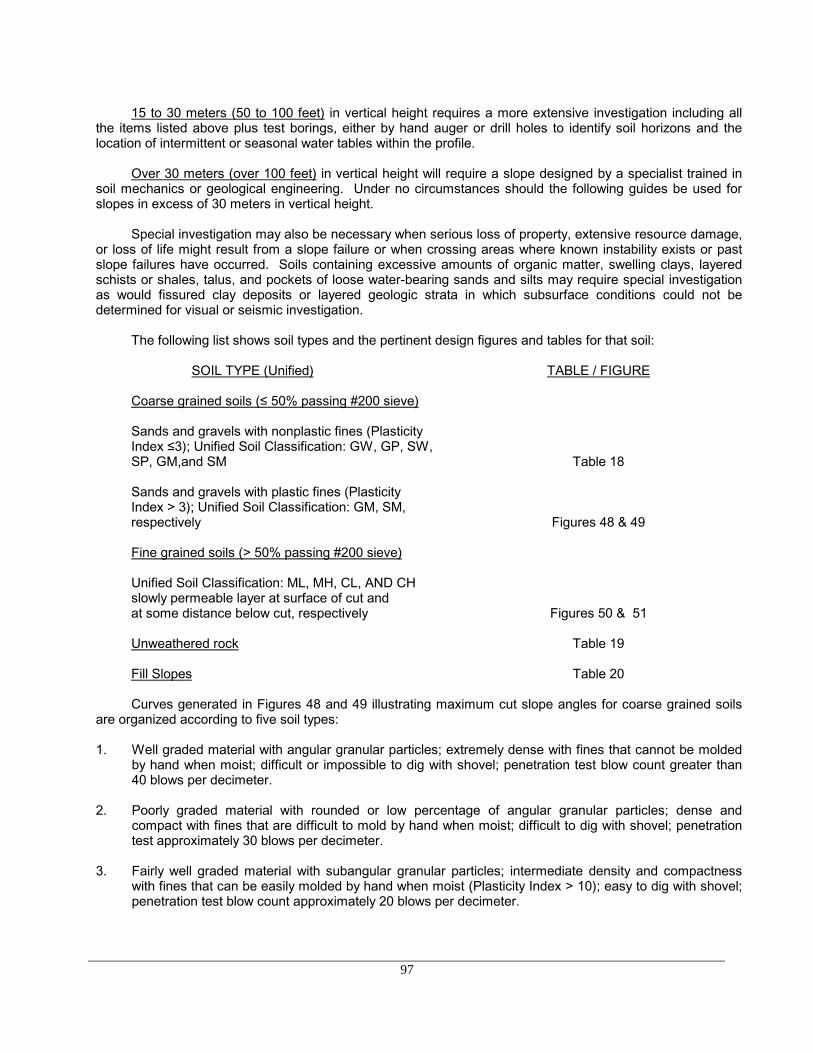
97

15 to 30 meters (50 to 100 feet) in vertical height requires a more extensive investigation including allthe items listed above plus test borings, either by hand auger or drill holes to identify soil horizons and thelocation of intermittent or seasonal water tables within the profile.

Over 30 meters (over 100 feet) in vertical height will require a slope designed by a specialist trained insoil mechanics or geological engineering. Under no circumstances should the following guides be used forslopes in excess of 30 meters in vertical height.

Special investigation may also be necessary when serious loss of property, extensive resource damage,or loss of life might result from a slope failure or when crossing areas where known instability exists or pastslope failures have occurred. Soils containing excessive amounts of organic matter, swelling clays, layeredschists or shales, talus, and pockets of loose water-bearing sands and silts may require special investigationas would fissured clay deposits or layered geologic strata in which subsurface conditions could not bedetermined for visual or seismic investigation.

The following list shows soil types and the pertinent design figures and tables for that soil:

SOIL TYPE (Unified) TABLE / FIGURE

Coarse grained soils (≤ 50% passing #200 sieve)

Sands and gravels with nonplastic fines (PlasticityIndex ≤3); Unified Soil Classification: GW, GP, SW,SP, GM,and SM Table 18

Sands and gravels with plastic fines (PlasticityIndex > 3); Unified Soil Classification: GM, SM,respectively Figures 48 & 49

Fine grained soils (> 50% passing #200 sieve)

Unified Soil Classification: ML, MH, CL, AND CHslowly permeable layer at surface of cut andat some distance below cut, respectively Figures 50 & 51

Unweathered rock Table 19

Fill Slopes Table 20

Curves generated in Figures 48 and 49 illustrating maximum cut slope angles for coarse grained soilsare organized according to five soil types:

1. Well graded material with angular granular particles; extremely dense with fines that cannot be moldedby hand when moist; difficult or impossible to dig with shovel; penetration test blow count greater than40 blows per decimeter.

2. Poorly graded material with rounded or low percentage of angular granular particles; dense andcompact with fines that are difficult to mold by hand when moist; difficult to dig with shovel; penetrationtest approximately 30 blows per decimeter.

3. Fairly well graded material with subangular granular particles; intermediate density and compactnesswith fines that can be easily molded by hand when moist (Plasticity Index > 10); easy to dig with shovel;penetration test blow count approximately 20 blows per decimeter.

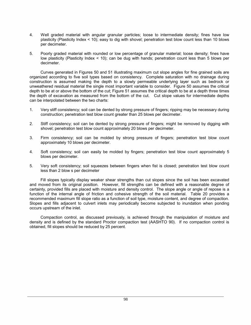
98

4. Well graded material with angular granular particles; loose to intermediate density; fines have lowplasticity (Plasticity Index < 10); easy to dig with shovel; penetration test blow count less than 10 blowsper decimeter.

5. Poorly graded material with rounded or low percentage of granular material; loose density; fines havelow plasticity (Plasticity Index < 10); can be dug with hands; penetration count less than 5 blows perdecimeter.

Curves generated in Figures 50 and 51 illustrating maximum cut slope angles for fine grained soils areorganized according to five soil types based on consistency. Complete saturation with no drainage duringconstruction is assumed making the depth to a slowly permeable underlying layer such as bedrock orunweathered residual material the single most important variable to consider. Figure 50 assumes the criticaldepth to be at or above the bottom of the cut; Figure 51 assumes the critical depth to be at a depth three timesthe depth of excavation as measured from the bottom of the cut. Cut slope values for intermediate depthscan be interpolated between the two charts:

1. Very stiff consistency; soil can be dented by strong pressure of fingers; ripping may be necessary duringconstruction; penetration test blow count greater than 25 blows per decimeter.

2. Stiff consistency; soil can be dented by strong pressure of fingers; might be removed by digging withshovel; penetration test blow count approximately 20 blows per decimeter.

3. Firm consistency; soil can be molded by strong pressure of fingers; penetration test blow countapproximately 10 blows per decimeter.

4. Soft consistency; soil can easily be molded by fingers; penetration test blow count approximately 5blows per decimeter.

5. Very soft consistency; soil squeezes between fingers when fist is closed; penetration test blow countless than 2 blow s per decimeter

Fill slopes typically display weaker shear strengths than cut slopes since the soil has been excavatedand moved from its original position. However, fill strengths can be defined with a reasonable degree ofcertainty, provided fills are placed with moisture and density control. The slope angle or angle of repose is afunction of the internal angle of friction and cohesive strength of the soil material. Table 20 provides arecommended maximum fill slope ratio as a function of soil type, moisture content, and degree of compaction.Slopes and fills adjacent to culvert inlets may periodically become subjected to inundation when pondingoccurs upstream of the inlet.

Compaction control, as discussed previously, is achieved through the manipulation of moisture anddensity and is defined by the standard Proctor compaction test (AASHTO 90). If no compaction control isobtained, fill slopes should be reduced by 25 percent.

99

table 24 Maximum cut slope ratio for coarse grained soils. (USFS, 1973)

--------------------------------------------------------------------------------------------------------------------------------

Soil Type Maximum Cut Slope Ratio (h:v)Low groundwater High groundwater 1/(below bottom of excavation)(seepage from entire slope)loose 2/ dense 3/ loose dense

GW, GP 1.5 : 1 .85 : 1 3 : 1 1.75 : 1

SW 1.6 : 1 1 : 1 3.2 : 1 2 : 1

GM, SP, SM 2 : 1 1.5 : 1 4 : 1 3 : 1--------------------------------------------------------------------------------------------------------------------------------1/ Based on material of saturated density approximately 19.6 kN/m3. Flatter slopes should be usedfor lower density material and steeper slopes can be used for higher density material. For every 5% change in density, change the ratio by approximately 5%.2/ Approximately 85% of maximum density.3/ Approximately 100% of maximum density.

table 25 Maximum cut slope ratio for bedrock excavation (USFS, 1973)

-------------------------------------------------------------------------------------------------------------------------------- Maximum Cut Slope Ratio

Rock type Massive Fractured--------------------------------------------------------------------------------------------------------------------------------Igneous (granite, trap, basalt, and volcanic tuff) 0.25:1 0.50:1

Sedimentary (massive sandstone and limestone; 0.25:1 0.50:1

interbedded sandstone, shale, and limestone; 0.50:1 0.75:1

massive claystone and siltstone) 0.75:1 1:1

Metamorphic (gneiss, schist, and marble; 0.25:1 0.50:1

slate; 0.50:1 0.75:1

(serpentine) Special investigation--------------------------------------------------------------------------------------------------------------------------------

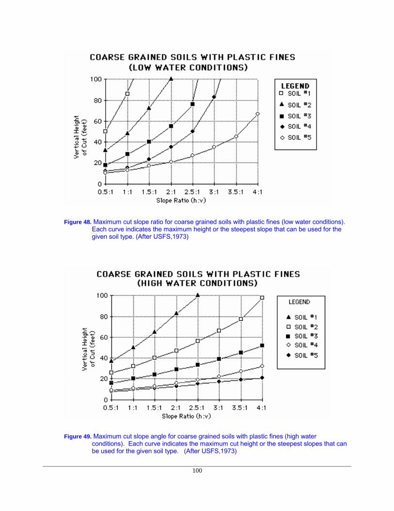
100

Figure 48. Maximum cut slope ratio for coarse grained soils with plastic fines (low water conditions).Each curve indicates the maximum height or the steepest slope that can be used for thegiven soil type. (After USFS,1973)

Figure 49. Maximum cut slope angle for coarse grained soils with plastic fines (high waterconditions). Each curve indicates the maximum cut height or the steepest slopes that canbe used for the given soil type. (After USFS,1973)

101

Figure 50. Maximum cut slope angle for fine grained soils with slowly permeable layer at bottom ofcut. Each curve indicates the maximum vertical cut height or the steepest slope that canbe used for the given soil type. (After USFS 1973)

102

FINE GRAINED SOILS WITH SLOWLY PERMEABLELAYER BELOW CUT (GREATER THAN

3X HEIGHT OF CUT)

--------------------------------------------------------------------------------------------------------------------------------Soil Type Maximum Height (m)1/ SlopeRatio (h:v)

1 24 0.5:1

2 2/ 12 0.5:1

3 2/ 6 0.5:1

4 3/ 3 1:1

5 3/ 1.5 1:1--------------------------------------------------------------------------------------------------------------------------------1/ If it is necessary to exceed this height consult with geologic or materials engineer.Benching will notimprove stability as stability is nearly independent of slope ratio on these slopes.

2/ If the slope of the natural ground exceeds 20° (36 percent), then the natural slope may beunstable. A detailed field investigation is necessary to check this condition prior to design orconstruction phases.

3/ If the slope of the natural ground exceeds 10° (18 percent), then the natural slope may beunstable. A detailed field investigation is necessary to check this condition prior to design orconstruction phases.--------------------------------------------------------------------------------------------------------------------------------

Figure 51. Maximum cut slope angle for fine grained soils with slowly permeable layer at great depth(> 3 times height of cut) below cut. (After USFS, 1973).

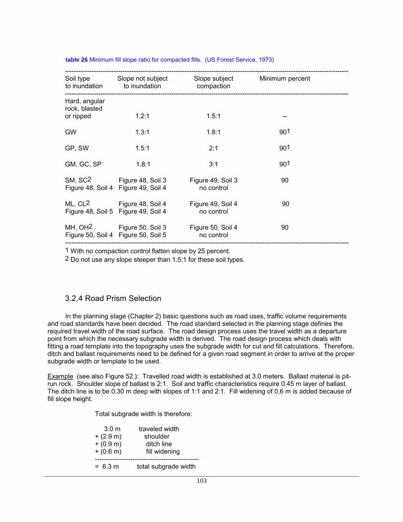
103

table 26 Minimum fill slope ratio for compacted fills. (US Forest Service, 1973)

--------------------------------------------------------------------------------------------------------------------------------Soil type Slope not subject Slope subject Minimum percentto inundation to inundation compaction--------------------------------------------------------------------------------------------------------------------------------Hard, angularrock, blastedor ripped 1.2:1 1.5:1 --

GW 1.3:1 1.8:1 901

GP, SW 1.5:1 2:1 901

GM, GC, SP 1.8:1 3:1 901

SM, SC2 Figure 48, Soil 3 Figure 49, Soil 3 90Figure 48, Soil 4 Figure 49, Soil 4 no control

ML, CL2 Figure 48, Soil 4 Figure 49, Soil 4 90Figure 48, Soil 5 Figure 49, Soil 4 no control

MH, OH2 Figure 50, Soil 3 Figure 50, Soil 4 90Figure 50, Soil 4 Figure 50, Soil 5 no control--------------------------------------------------------------------------------------------------------------------------------1 With no compaction control flatten slope by 25 percent.2 Do not use any slope steeper than 1.5:1 for these soil types.

3.2.4 Road Prism Selection

In the planning stage (Chapter 2) basic questions such as road uses, traffic volume requirementsand road standards have been decided. The road standard selected in the planning stage defines therequired travel width of the road surface. The road design process uses the travel width as a departurepoint from which the necessary subgrade width is derived. The road design process which deals withfitting a road template into the topography uses the subgrade width for cut and fill calculations. Therefore,ditch and ballast requirements need to be defined for a given road segment in order to arrive at the propersubgrade width or template to be used.

Example (see also Figure 52.): Travelled road width is established at 3.0 meters. Ballast material is pit-run rock. Shoulder slope of ballast is 2:1. Soil and traffic characteristics require 0.45 m layer of ballast.The ditch line is to be 0.30 m deep with slopes of 1:1 and 2:1. Fill widening of 0,6 m is added because offill slope height.

Total subgrade width is therefore:

3.0 m traveled width+ (2.9 m) shoulder+ (0.9 m) ditch line+ (0.6 m) fill widening-----------------------------------------------

= 6.3 m total subgrade width

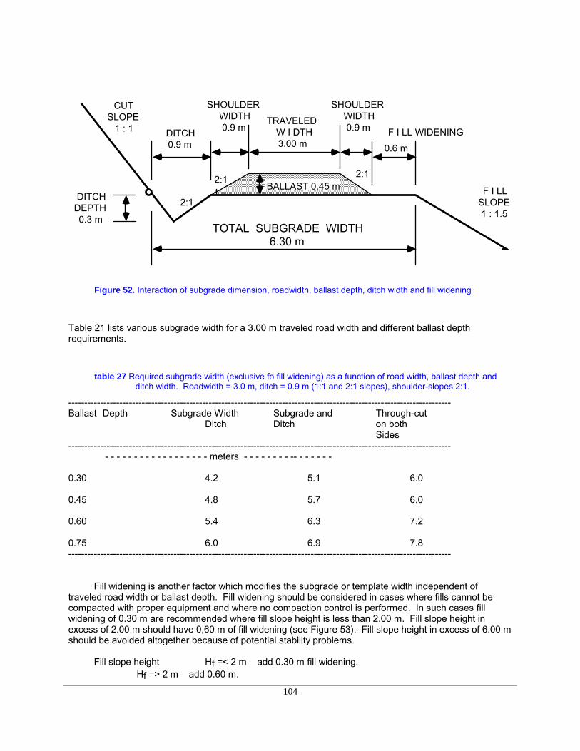
104

DITCH 0.9 m

SHOULDER WIDTH 0.9 m

SHOULDER WIDTH 0.9 m

TRAVELED W I DTH 3.00 m

F I LL WIDENING0.6 m

CUT SLOPE

1 : 1

DITCH DEPTH 0.3 m

2:1

2:1 2:1

F I LL SLOPE 1 : 1.5

TOTAL SUBGRADE WIDTH 6.30 m

BALLAST 0.45 m

Figure 52. Interaction of subgrade dimension, roadwidth, ballast depth, ditch width and fill widening

Table 21 lists various subgrade width for a 3.00 m traveled road width and different ballast depthrequirements.

table 27 Required subgrade width (exclusive fo fill widening) as a function of road width, ballast depth andditch width. Roadwidth = 3.0 m, ditch = 0.9 m (1:1 and 2:1 slopes), shoulder-slopes 2:1.

------------------------------------------------------------------------------------------------------------------------Ballast Depth Subgrade Width Subgrade and Through-cut

Ditch Ditch on bothSides

------------------------------------------------------------------------------------------------------------------------ - - - - - - - - - - - - - - - - - - meters - - - - - - - - -- - - - - - -

0.30 4.2 5.1 6.0

0.45 4.8 5.7 6.0

0.60 5.4 6.3 7.2

0.75 6.0 6.9 7.8------------------------------------------------------------------------------------------------------------------------

Fill widening is another factor which modifies the subgrade or template width independent oftraveled road width or ballast depth. Fill widening should be considered in cases where fills cannot becompacted with proper equipment and where no compaction control is performed. In such cases fillwidening of 0.30 m are recommended where fill slope height is less than 2.00 m. Fill slope height inexcess of 2.00 m should have 0,60 m of fill widening (see Figure 53). Fill slope height in excess of 6.00 mshould be avoided altogether because of potential stability problems.

Fill slope height Hf =< 2 m add 0.30 m fill widening.Hf => 2 m add 0.60 m.

105

Maximum Fill slope height Hf =< 6.00 m (unless engineered)

Cut slopes are inherently more stable than fill slopes. The road designer should try to minimize fillslope length by "pushing the alignment into the hill side in order to minimize erosion. Typically this willresult in longer cut slopes and add slight to moderate cuts at the center line. The result will be a moderatefill slope (see Figure 54) with no additional fill widening required.

Toe walls are often a feasible alternative on steep side slopes to reduce excavation and avoid endhauling. Toe walls can be built of log cribs, gabions or large rocks (Figure 55). A proper base foundationis excavated at the toe of the fill on which the retaining wall is constructed. Approximately two-thirds of thesubgrade would be projected into the hill side and one third would be supported by the fill resting on theretaining structure.The reduction in excavation material, exposed cut slope and avoided end haul issignificant.

STANDARD SUBGRADE

FILL WIDENING

FILL SLOPE HEIGHT

STANDARD SUBGRADE

FILL WIDENING

FILL WIDENING

FILL SLOPE HEIGHT

FILL WIDENING

Figure 53. Fill widening added to standard subgrade width where fill height at centerline or shoulderexceeds a critical height. Especially important if sidecast construction instead of layerconstruction is used.

106

C L C L

FILL SLOPE LENGTH REDUCTION

Figure 54. Template and general road alignment projected into the hill favoring light to moderatecuts at centerline in order to minimize fill slope length. Fill slopes are more succeptible toerosion and sloughing than cut slopes.

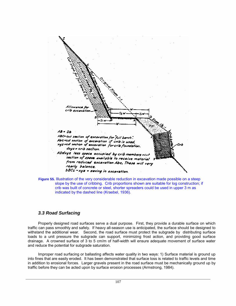
107

Figure 55. Illustration of the very considerable reduction in excavation made possible on a steepslope by the use of cribbing. Crib proportions shown are suitable for log construction; ifcrib was built of concrete or steel, shorter spreaders could be used in upper 3 m asindicated by the dashed line (Kraebel, 1936).

3.3 Road Surfacing

Properly designed road surfaces serve a dual purpose. First, they provide a durable surface on whichtraffic can pass smoothly and safely. If heavy all-season use is anticipated, the surface should be designed towithstand the additional wear. Second, the road surface must protect the subgrade by distributing surfaceloads to a unit pressure the subgrade can support, minimizing frost action, and providing good surfacedrainage. A crowned surface of 3 to 5 cm/m of half-width will ensure adequate movement of surface waterand reduce the potential for subgrade saturation.

Improper road surfacing or ballasting affects water quality in two ways: 1) Surface material is ground upinto fines that are easily eroded. It has been demonstrated that surface loss is related to traffic levels and timein addition to erosional forces. Larger gravels present in the road surface must be mechanically ground up bytraffic before they can be acted upon by surface erosion processes (Armstrong, 1984).

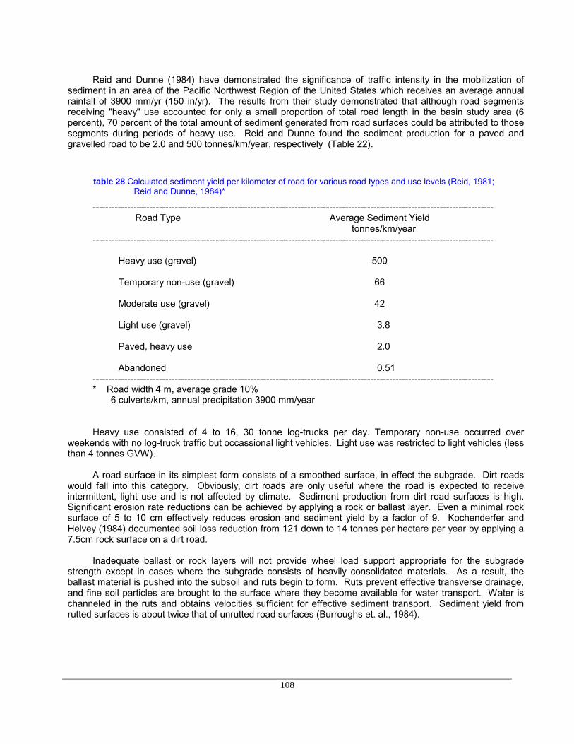
108

Reid and Dunne (1984) have demonstrated the significance of traffic intensity in the mobilization ofsediment in an area of the Pacific Northwest Region of the United States which receives an average annualrainfall of 3900 mm/yr (150 in/yr). The results from their study demonstrated that although road segmentsreceiving "heavy" use accounted for only a small proportion of total road length in the basin study area (6percent), 70 percent of the total amount of sediment generated from road surfaces could be attributed to thosesegments during periods of heavy use. Reid and Dunne found the sediment production for a paved andgravelled road to be 2.0 and 500 tonnes/km/year, respectively (Table 22).

table 28 Calculated sediment yield per kilometer of road for various road types and use levels (Reid, 1981;Reid and Dunne, 1984)*

-------------------------------------------------------------------------------------------------------------------------------Road Type Average Sediment Yield

tonnes/km/year-------------------------------------------------------------------------------------------------------------------------------

Heavy use (gravel) 500

Temporary non-use (gravel) 66

Moderate use (gravel) 42

Light use (gravel) 3.8

Paved, heavy use 2.0

Abandoned 0.51-------------------------------------------------------------------------------------------------------------------------------* Road width 4 m, average grade 10% 6 culverts/km, annual precipitation 3900 mm/year

Heavy use consisted of 4 to 16, 30 tonne log-trucks per day. Temporary non-use occurred overweekends with no log-truck traffic but occassional light vehicles. Light use was restricted to light vehicles (lessthan 4 tonnes GVW).

A road surface in its simplest form consists of a smoothed surface, in effect the subgrade. Dirt roadswould fall into this category. Obviously, dirt roads are only useful where the road is expected to receiveintermittent, light use and is not affected by climate. Sediment production from dirt road surfaces is high.Significant erosion rate reductions can be achieved by applying a rock or ballast layer. Even a minimal rocksurface of 5 to 10 cm effectively reduces erosion and sediment yield by a factor of 9. Kochenderfer andHelvey (1984) documented soil loss reduction from 121 down to 14 tonnes per hectare per year by applying a7.5cm rock surface on a dirt road.

Inadequate ballast or rock layers will not provide wheel load support appropriate for the subgradestrength except in cases where the subgrade consists of heavily consolidated materials. As a result, theballast material is pushed into the subsoil and ruts begin to form. Ruts prevent effective transverse drainage,and fine soil particles are brought to the surface where they become available for water transport. Water ischanneled in the ruts and obtains velocities sufficient for effective sediment transport. Sediment yield fromrutted surfaces is about twice that of unrutted road surfaces (Burroughs et. al., 1984).

109

An improvement over a simple dirt road consists of a ballast layer over a subgrade, with or without awearing course. The function of the ballast layer is to distribute the wheel load to pressures the subsoil canwithstand. The wearing course provides a smooth running surface and also seals the surface to protect thesubgrade from surface water infiltration. The wearing course can either be a crushed gravel layer with fines ora bitumenous layer.

Required ballast depth or thickness not only depends on subgrade strength but also on vehicle weightand traffic volume. The time or service life a road can support traffic without undue sediment delivery dependson:

- soil strength- ballast depth- traffic volume (number of axles)- vehicle weight (axle load)

Surface loading from wheel pressure is transmitted through the surface to the subgrade in the form of afrustrum of a cone. Thus, the unit pressure on the subgrade decreases with increasing thickness of thepavement structure. Average unit pressure across the entire width of subgrade for any wheel loadconfiguration can be calculated from the following formula:

P = L / π(r+d)2

Where: P = unit pressure (kN/cm2)L = wheel load (kN)r = radius of circle, equal in area to tire contact area (cm)d = depth of pavement structure (cm)

A useful parameter for determining the strength of subgrade material is the California Bearing Ratio(CBR). CBR values are indices of soil strength and swelling potential. They represent the ratio of theresistance of a compacted soil to penetration by a test piston to penetration resistance of a "standardmaterial", usually compacted, crushed rock (Atkins, 1980). The range of CBR values for natural soils is listedin Table 23 together with their suitability as subgrade material. Poorer subgrade material requires a thickerballast layer to withstand traffic load and volume.

Factors other than CBR values must be considered when determining the thickness of the pavementstructure. Subgrade compaction will depend upon construction methods used and the control of moistureduring compaction. Subgrade drainage effectiveness, frost penetration and frost heave, and subgrade soilswell pressure are associated with water content in the soil and will also affect final design thickness. Tocounteract these factors, a thicker, heavier pavement structure should be designed.

110

table 29 Engineering characteristics of soil groups for road construction (Pearce, 1960).

------------------------------------------------------------------------------------------------------------------------------------ Unified Soil Field CBR Dry weight* Frost

Suitability Classification Value (kN/m3) Action

Subgrade**

GW 60-80 19.6-22 none to excellentvery slight

GP 25-60 17.3-20.4 none to good to excellentvery slight

GM-d*** 40-80 20.4-22.8 slight to good to excellentmedium

GM-u*** 20-40 18.9-22 slight to goodmedium

GC 20-40 18.9-22 slight to goodmedium

SW 20-40 17.3-20.4 none to goodvery slight

SP 10-25 15.7-18.9 none to fairvery slight

SM-d*** 20-40 18.9-21.2 slight to good high

SM-u*** 10-20 16.5-20.4 slight to fair to good high

SC 10-20 16.5-20.4 slight to fair to good high

ML 5-15 15.7-19.6 medium to fair to poorvery high

CL 5-15 15.7-19.6 medium to fair to poor high

OL 4-8 14.1-16.5 medium to poor high

MH 4-8 12.6-15.7 medium to poorvery high

CH 3-5 14.1-17.3 medium poor to very poorOH 3-5 12.6-16.5 medium poor to very poor

PT slight unsuitable------------------------------------------------------------------------------------------------------------------------------------* Unit dry weight for compacted soil at optimum moisture content for modified AASTO compactive effort.** Value as subgrade, foundation or base course (except under bituminous) when not subject to frostaction.*** "d" = liquid limit ≤ 28 and plasticity index < 6; "u" = liquid limit > 28.

111

An alternative to the cost of a heavier pavement structure is the use of geotextile fabrics. Fabrics havebeen found to be an economically acceptable alternative to conventional construction practices when dealingwith less than desirable soil material. The U. S. Forest Service has successfully used fabrics as filters forsurface drainage, as separatory features to prevent subgrade soil contamination of base layers, and assubgrade restraining layers for weak subgrades. A useful guide for the selection and utilization of fabrics inconstructing and maintaining low volume roads is presented by Steward, et al. (1977). This report discussesthe current knowledge regarding the use of fabrics in road construction and contains a wealth of informationregarding physical properties and costs of several brands of fabric currently marketed in the United States andabroad.

Proper thickness design of ballast layer not only helps to reduce erosion but also reduces costs byrequiring only so much rock as is actually required by traffic volume (number of axles) and vehicle weight (axleweight-wheel loads). The principle of thickness design is based on the system developed by AASHO(American Association of State Highway Officials) and adapted by Barenberg et al. (1975) to soft soils.Barenberg developed a relationship between required ballast thickness and wheel or axle loads. Soil strengthcan be simply measured either with a cone penetrometer or vane shear device, such as a Torvane.

Thickness design for soft soil is based on the assumption of foundation shear failure where the bearingcapacity of the soil is exceeded. For rapid loading, such as the passage of a wheel, the bearing capacity q isassumed to depend on cohesion only.

q = Nc * Cwhere q = Bearing capacity of a soil (kg/cm2).

C = Cohesive strength of soil (kg/cm2).Nc = Dimensionless bearing capacity factor

Based on Barenberg's work, Steward, et al. (1977) proposed a value of 2.8 to 3.3 and 5.0 to 6.0 for Nc.The significance of the bearing capacity q is as follows:

A. q = 2.8 C is the stress level on the subgrade at which very little rutting will occur under heavy traffic (morethan 1000 trips of 8,160 kg axle equivalencies) without fabric.

B. q = 3.3 C is the stress level at which heavy rutting will occur under light axle loadings (less than 100 trips of8,160 kg axle equivalencies) without fabric.

C. q = 5.0 C is the stress level at which very little rutting would be expected to occur at high traffic volumes(more than 1000 trips of 8,160 kg equivalency axles) using fabric.

D. q = 6.0 C is the stress level at which heavy rutting will occur under light axle loadings (less than 100 trips of8,160 kg axle equivalencies) using fabric.

(Heavy rutting is defined as ruts having a depth of 10 cm or greater. Very little rutting is defined as ruts havinga depth of less than 5 cm extending into the subgrade.)

Charts relating soil strength (as measured with a vane shear device) to axle load and ballast thicknessare shown in Figure 56 through 58. Figure 56 is based on a single axle, single wheel load. Figure 57 is basedon a double wheel, single axle load, and Figure 58 is based on a tandem wheel configuration typical of 3 axledump trucks or stinger type log-trucks.

It should be noted that axle and wheel configuration have a tremendous impact on the load bearingcapacity of a road. The relationship between axle load and subgrade failure is not linear. Allowing 16,000 kgaxle load vehicle to use a road designed for a standard axle load of 8,200 kg, is equivalent to 15 trips with the8,200 kg axle load vehicle. Premature rut formation and its prevention depend on the selection of the properaxle load and strict enforcement of the selected load standard.

112

Some typical truck configurations, gross vehicle weights (GVW), and axle or wheel loads are given inTable 24. Vehicles under 3 tonnes GVW have no measurable effect on subgrade stress and deterioration.

Design Example

A road is to be constructed to access a watershed. Because of erosive conditions and traffic volumes,only 5 cm of rutting can be tolerated. Expected traffic volume is high (greater than 1,000 axle loads).

Three vehicle types are using the road:

1. Utility truck - 10 tonnes GVW; 4,500 kg single wheel load (9,000 kg axle load on rear axle, loaded)

2. Dump truck - 15 tonnes GVW with two axles;(11 tonnes rear axle load or 5.5 tonnes per dual wheel)

3. Log truck - 36 tonnes GVW with 5 axles, rear tandem axle load

equals 15.9 tonnes or 7.95 tonnes per tandem wheel set.

Soil tests: Visually segment the road into logical construction segments based on soil type. Take soil strengthmeasurements with vane shear device. Measurements should be taken during wet soilconditions, its weakest state. Take at least 10 vane shear readings at approximately 10 cm and40 cm below the surface (in mineral soil). Tabulate readings in descending order from largest tosmallest value. Your design shear strength is the 25th percentile shear strength--the value atwhich 75 percent of the soil strength readings are higher.

Vane Shear Readings1. 0.58 kg/cm22. 0.583. 0.504. 0.465. 0.456. 0.457. 0.408. 0.379. 0.36 => 0.36 (25 percentile) -Design strength to be 10.0.32 used in calculation.11. 0.3212. 0.30

Subgrade strength for design purpose is taken as 0.36 kg/cm2.

Ballast Depth Calculation: Calculate the soil stress value without fabric for little rutting (less than 5 cm for morethan 1,000 axle loads).

q = 2.8 * 0.36 = 1.01 kg/cm2

(Conversion factor: Multiply kg/cm2 by 14.22 to get psi. This gives a value of 14.33 psi in this example).

In the case of the utility truck with 4,500 kg (10,000 lbs) wheel load, enter Figure 56 at 14.33 on thebottom line and read upwards to the 4,500 kg (10,000 lbs) single wheel load. A reading of 42 cm (16.5 in.) isobtained. Since 7 -12 cm additional ballast is needed to compensate for intrusion from the soft subgrade, atotal of 49 - 54 cm of ballast is required. When fabric is used, a factor of 5.0 (little rutting for high trafficvolumes) is applied to determine the ballast depth.

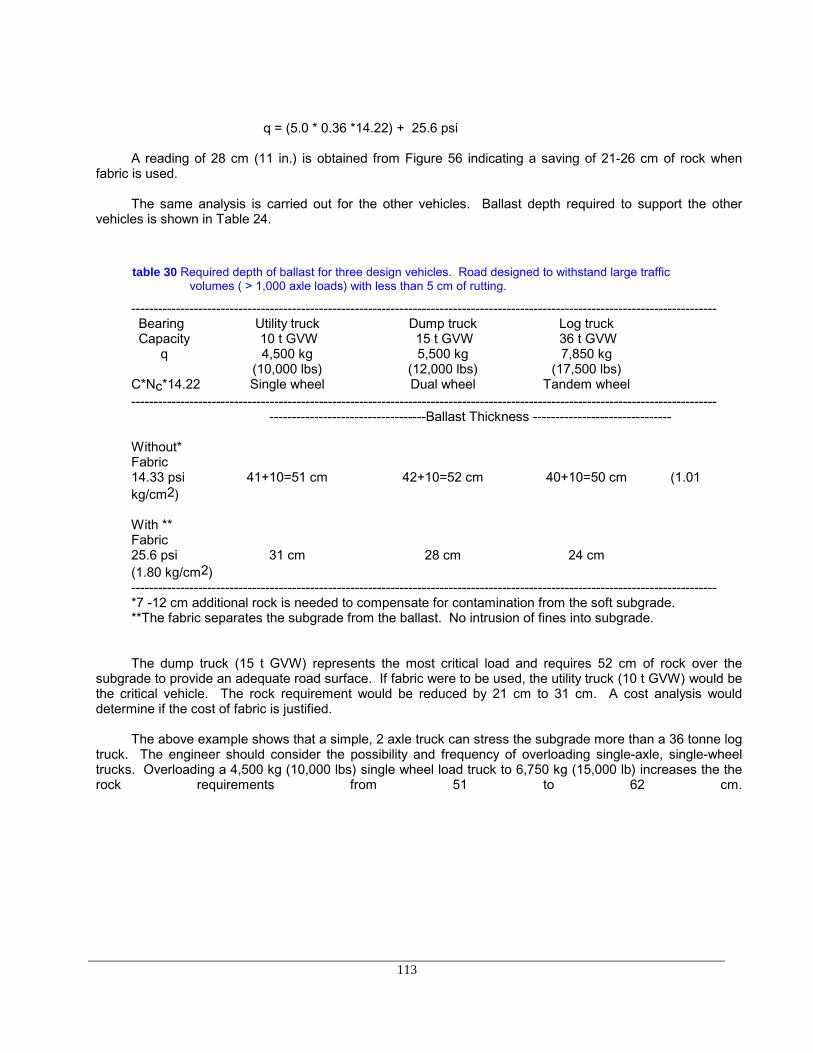
113

q = (5.0 * 0.36 *14.22) + 25.6 psi

A reading of 28 cm (11 in.) is obtained from Figure 56 indicating a saving of 21-26 cm of rock whenfabric is used.

The same analysis is carried out for the other vehicles. Ballast depth required to support the othervehicles is shown in Table 24.

table 30 Required depth of ballast for three design vehicles. Road designed to withstand large trafficvolumes ( > 1,000 axle loads) with less than 5 cm of rutting.

----------------------------------------------------------------------------------------------------------------------------------- Bearing Utility truck Dump truck Log truck Capacity 10 t GVW 15 t GVW 36 t GVW q 4,500 kg 5,500 kg 7,850 kg

(10,000 lbs) (12,000 lbs) (17,500 lbs)C*Nc*14.22 Single wheel Dual wheel Tandem wheel-----------------------------------------------------------------------------------------------------------------------------------

-----------------------------------Ballast Thickness -------------------------------

Without*Fabric14.33 psi 41+10=51 cm 42+10=52 cm 40+10=50 cm (1.01kg/cm2)

With **Fabric25.6 psi 31 cm 28 cm 24 cm(1.80 kg/cm2)-----------------------------------------------------------------------------------------------------------------------------------*7 -12 cm additional rock is needed to compensate for contamination from the soft subgrade.**The fabric separates the subgrade from the ballast. No intrusion of fines into subgrade.

The dump truck (15 t GVW) represents the most critical load and requires 52 cm of rock over thesubgrade to provide an adequate road surface. If fabric were to be used, the utility truck (10 t GVW) would bethe critical vehicle. The rock requirement would be reduced by 21 cm to 31 cm. A cost analysis woulddetermine if the cost of fabric is justified.

The above example shows that a simple, 2 axle truck can stress the subgrade more than a 36 tonne logtruck. The engineer should consider the possibility and frequency of overloading single-axle, single-wheeltrucks. Overloading a 4,500 kg (10,000 lbs) single wheel load truck to 6,750 kg (15,000 lb) increases the therock requirements from 51 to 62 cm.

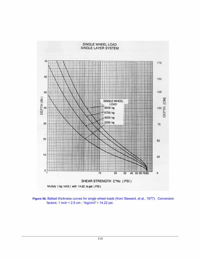
114

Figure 56. Ballast thickness curves for single wheel loads (from Steward, et al., 1977). Conversionfactors: 1 inch = 2.5 cm ; 1kg/cm2 = 14.22 psi.

115

Figure 57. Ballast thickness curves for dual wheel loads (from Steward, et al., 1977). Conversionfactors: 1 inch = 2.5 cm ; 1kg/cm2 = 14.22 psi.

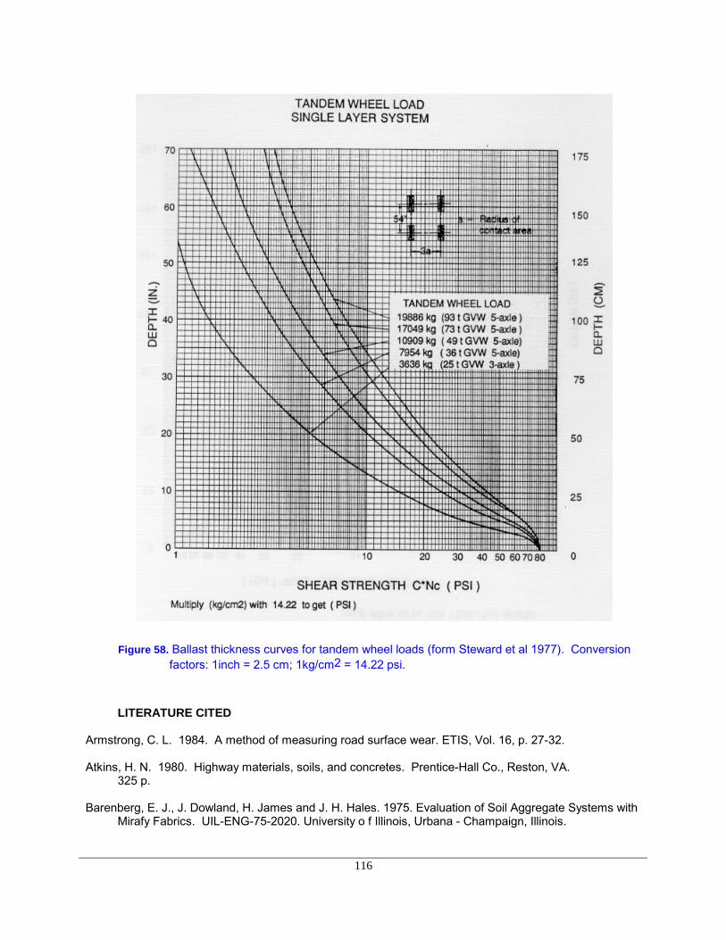
116

Figure 58. Ballast thickness curves for tandem wheel loads (form Steward et al 1977). Conversionfactors: 1inch = 2.5 cm; 1kg/cm2 = 14.22 psi.

LITERATURE CITED

Armstrong, C. L. 1984. A method of measuring road surface wear. ETIS, Vol. 16, p. 27-32.

Atkins, H. N. 1980. Highway materials, soils, and concretes. Prentice-Hall Co., Reston, VA.325 p.

Barenberg, E. J., J. Dowland, H. James and J. H. Hales. 1975. Evaluation of Soil Aggregate Systems withMirafy Fabrics. UIL-ENG-75-2020. University o f Illinois, Urbana - Champaign, Illinois.

117

Bishop, A. W. 1950. Use of the slip circle inslope stability analysis. Geotechnique 5(1):7-17.

Burroughs, Jr., E. R., G. R. Chalfant and M. A. Townsend. 1976. Slope stability in road construction. U. S.Dept. of Interior, Bureau of Land Management and Montana State University. Portland, Oregon. 102 p.

Burroughs , Jr.,E. R., F. J. Watts and D.F. Haber. 1984. Surfacing to reduce erosion of forest roads built ingranitic soils. In: Symposium on effects of forest landslides on erosion and slope stability. May 1984.University of Hawaii, p. 255 - 264.

Cain, C. 1981. Maximum grades for log trucks on forest roads. Eng. Field Notes. Vol. 13, No. 6, 1981. USDAForest Service, Eng. Techn. Inf. Syst., Washington D.C.

Cain, C. and J. A. Langdon. 1982. A guide for determining road width on curves for single-lane forest roads.Eng. Field Notes. Vol. 14, No. 4-6, 1982. USDA Forest Service, Eng. Techn. Inf. Syst., WashingtonD.C.

Chen, W. F. and M. W. Giger. 1971. Limit analysis of stability of slopes. J. Soil Mechanics and FoundationsDiv., Proc. ASCE, Vol. 97, No. Sm1, Proc. Paper 7828, Jan. 1971, pp. 19-26.

Dietz, R., W. Knigge and H. Loeffler, 1984. Walderschliessung. Verlag Paul Parey,Hamburg, Germany, pp.426.

Kochenderfer, J. N. and J. D. Helvey. 1984. Soil losses from a minimum-standard truck road constructed inthe Appalachians. In: Mountain Logging Symposium (ed. P. Peters and J. Luchok) West VirginiaUniversity. Morgantown, W. Virginia. p. 215-275.

Kraebel, C. 1936. Erosion control on mountain roads. USDA Circular No. 380, Washington D. C. 44 pp.

Kramer, B. 1982. Vehicle tracking simulation techniques for low speed forest roads in the Pacific Northwest.ASAE No. PNR - 82 - 508. St. Joseph, Michigan.

Kuonen, V. 1983. Wald-und Gueterstrassen Eigenverlag, Pfaffhausen, Switzerland. 743 pp.

Ohmstede, R. 1976. Vertical curves and their influence on the performance of log trucks. Eng. Field Notes.Vol. 8, No. 11, 1976. USDA Forest Service, Eng. Techn. Inf. Syst., Washington D.C.

Pearce, J. K. 1960. Forest Engineering Handbook. Prepared for U. S. Department of the Interior, Bureau ofLand Management. 220 pp.

Prellwitz,R. W. 1975. Simplified slope design for low volume roads in mountaineous areas. In: Low volumeroads. Proceedings, June 1975. Special Report 160. Transp. Research Board, National Academy ofSciences, Washington,D.C., pp. 65-74.

Reid, L. M. 1981. Sediment production from gravel-surfaced forest roads, Clearwater Basin, Washington.Publ. FRI-UW-8108, Univ. of Washington, Seattle. 247 p.

Reid, L. M. and T. Dunne. 1984. Sediment production from forest road surfaces. Water ResourcesResearch 20:1753-61.

Steward, J. E., R. Williamson, and J. Mohney. 1977. Guidelines for use of fabrics in construction andmaintenance of low volume roads. Nat. Tech. Info. Svc. Springfield, VA 22161. 172 pp.

USDA, Forest Service. 1973. Transportation Engineering Handbook, Slope design guide. Handbook No.7709.11.

118

CHAPTER 4

DRAINAGE DESIGN

4.1 General Considerations

Roads will affect the natural surface and subsurface drainage pattern of a watershed or individualhillslope. Road drainage design has as its basic objective the reduction and/or elimination of energygenerated by flowing water. The destructive power of flowing water, as stated in Section 3.2.2, increasesexponentially as its velocity increases. Therefore, water must not be allowed to develop sufficient volume orvelocity so as to cause excessive wear along ditches, below culverts, or along exposed running surfaces, cuts,or fills.

Provision for adequate drainage is of paramount importance in road design and cannot beoveremphasized. The presence of excess water or moisture within the roadway will adversely affect theengineering properties of the materials with which it was constructed. Cut or fill failures, road surface erosion,and weakened subgrades followed by a mass failure are all products of inadequate or poorly designeddrainage. As has been stated previously, many drainage problems can be avoided in the location and designof the road. Drainage design is most appropriately included in alignment and gradient planning.

Hillslope geomorphology and hydrologic factors are important considerations in the location, design, andconstruction of a road. Slope morphology impacts road drainage and ultimately road stability. Importantfactors are slope shape (uniform, convex, concave), slope gradient, slope length, stream drainagecharacteristics (e.g., braided, dendritic), depth to bedrock, bedrock characteristics (e.g., fractured, hardness,bedding), and soil texture and permeability. Slope shape (Figure 59 gives an indication of surface andsubsurface water concentration or dispersion. Convex slopes (e.g., wide ridges) will tend to disperse water asit moves downhill. Straight slopes concentrate water on the lower slopes and contribute to the buildup ofhydrostatic pressure. Concave slopes typically exhibit swales and draws. Water in these areas isconcentrated at the lowest point on the slope and therefore represents the least desirable location for a road.

Hydrologic factors to consider in locating roads are: number of stream crossings, side slope, andmoisture regime. For example, at the lowest point on the slope, only one or two stream crossings may berequired. Likewise, side slopes generally are not as steep, thereby reducing the amount of excavation.However, side cast fills and drainage requirements will need careful attention since water collected from upperpositions on the slope will concentrate in the lower positions. In general, roads built on the upper one-third ofa slope have better soil moisture conditions and, therefore, tend to be more stable than roads built on lowerpositions on the slope.

Natural drainage characteristics of a hillslope, as a rule, should not be changed. For example, adrainage network will expand during a storm to include the smallest depression and draw in order to collectand transport runoff. Therefore, a culvert should be placed in each draw so as not to impede the naturaldisposition of stormflow. Culverts should be placed at grade and in line with the centerline of the channel.Failure to do this often results in excessive erosion of soils above and below the culvert. Also, debris cannotpass freely through the culvert causing plugging and oftentimes complete destruction of the road prism.Headwater streams are of particular concern (point A, Figure 60) since it is common to perceive thatmeasurable flows cannot be generated from the moisture collection area above the crossings. However, littleor no drainage on road crossings in these areas is notorious for causing major slide and debris torrents,especially if they are located on convex slope breaks.

Increased risks of road failures are created at points A and B. At point A, water will pond above the roadfill or flow downslope through the roadside ditch to point B. Ponding at A may cause weakening and/or

119

erosion of the subgrade . If the culvert on Stream 1 plugs, water and debris will flow to point A and from A toB. Hence, the culvert at B is handling discharge from all

CONVEX SLOPE

STRAIGHT OR PARALLEL SLOPES

CONCAVE SLOPE

Figure 59. Slope shape and its impact on slope hydrology. Slope shape determines whether wateris dispersed or concentrated. (US Forest Service,1979)

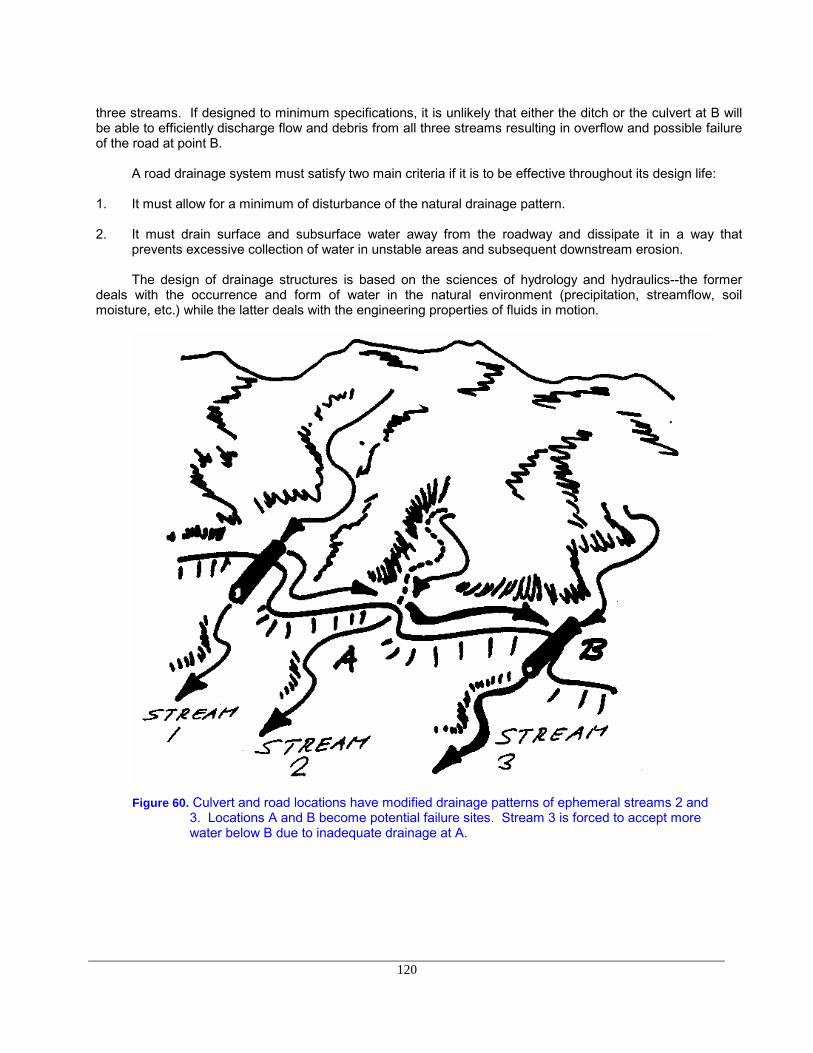
120

three streams. If designed to minimum specifications, it is unlikely that either the ditch or the culvert at B willbe able to efficiently discharge flow and debris from all three streams resulting in overflow and possible failureof the road at point B.

A road drainage system must satisfy two main criteria if it is to be effective throughout its design life:

1. It must allow for a minimum of disturbance of the natural drainage pattern.

2. It must drain surface and subsurface water away from the roadway and dissipate it in a way thatprevents excessive collection of water in unstable areas and subsequent downstream erosion.

The design of drainage structures is based on the sciences of hydrology and hydraulics--the formerdeals with the occurrence and form of water in the natural environment (precipitation, streamflow, soilmoisture, etc.) while the latter deals with the engineering properties of fluids in motion.

Figure 60. Culvert and road locations have modified drainage patterns of ephemeral streams 2 and3. Locations A and B become potential failure sites. Stream 3 is forced to accept morewater below B due to inadequate drainage at A.

121

4.2 Estimating runoff

Any drainage installation is sized according to the probability of occurrence of an expected peakdischarge during the design life of the installation. This, of course, is related to the intensity and duration ofrainfall events occurring not only in the direct vicinity of the structure, but also upstream of the structure. Insnow zones, peak discharge may be the result of an intense warming period causing rapid melting of thesnowpack.

In addition to considering intensity and duration of a peak rainfall event, the frequency, or how often thedesign maximum may be expected to occur, is also a consideration and is most often based on the life of theroad, traffic, and consequences of failure. Primary highways often incorporate frequency periods of 50 to 100years, secondary roads 25 years, and low volume forest roads 10 to 25 years.

Of the water that reaches the ground in the form of rain, some will percolate into the soil to be storeduntil it is taken up by plants or transported through pores as subsurface flow, some will evaporate back intothe atmosphere, and the rest will contribute to overland flow or runoff. Streamflow consists of stored soilmoisture which is supplied to the stream at a more or less constant rate throughout the year in the form ofsubsurface or groundwater flow plus water which is contributed to the channel more rapidly as the drainagenet expands into ephemeral channels to incorporate excess rainfall during a major storm event. Theproportion of rainfall that eventually becomes streamflow is dependent on the following factors:

1. The size of the drainage area. The larger the area, the greater the volume of runoff. An estimate of basinarea is needed in order to use runoff formulas and charts.

2. Topography. Runoff volume generally increases with steepness of slope. Average slope, basin elevation,and aspect, although not often called for in most runoff formulas and charts, may provide helpful cluesin refining a design.

3. Soil. Runoff varies with soil characteristics, particularly permeability and infiltration capacity. Theinfiltration rate of a dry soil, by nature of its intrinsic permeability, will steadily decrease with time as itbecomes wetted, given a constant rainfall rate. If the rainfall rate is greater than the final infiltration rateof the soil (infiltration capacity), that quantity of water which cannot be absorbed is stored in depressionsin the ground or runs off the surface. Any condition which adversely affects the infiltrationcharacteristics of the soil will increase the amount of runoff. Such conditions may includehydrophobicity, compaction, and frozen earth.

A number of different methods are available to predict peak flows. Flood frequency analysis is the mostaccurate method employed when sufficient hydrologic data is available. For instance, the United StatesGeological Survey has published empirical equations providing estimates of peak discharges from streams inmany parts of the United States based on regional data collected from "gauged" streams. In northwestOregon, frequency analysis has revealed that discharge for the flow event having a 25-year recurrence intervalis most closely correlated with drainage area and precipitation intensity for the 2-year, 24-hour storm event.This is, by far, the best means of estimating peak flows on an ungauged stream since the recurrence intervalassociated with any given flow event can be identified and used for evaluating the probability of failure.

The probability of occurrence of peak flows exceeding the design capacity of a proposed streamcrossing installation should be determined and used in the design procedure. To incorporate this informationinto the design, the risk of failure over the design life must be specified. By identifying an acceptable level ofrisk, the land manager is formally stating the desired level of success (or failure) to be achieved with roaddrainage structures. Table 25 lists flood recurrence intervals for installations in relation to their design life andprobability of failure.

table 31 Flood recurrence interval (years) in relation to design life and probability of failure.* (Megahan, 1977)

122

------------------------------------------------------------------------------------------------------------------------------------Design Life Chance of Failure ( % )

----------------------------------------------------------------------------------------------------- (years) 10 20 30 40 50 60 70------------------------------------------------------------------------------------------------------------------------------------

-------------------Recurrence Interval (years)----------------------

5 48 23 15 10 8 6 510 95 45 29 20 15 11 915 100+ 68 43 30 22 17 1320 100+ 90 57 40 229 22 1725 200+ 100+ 71 49 37 28 2130 200+ 100+ 85 59 44 33 2540 300+ 100+ 100+ 79 58 44 3450 400+ 200+ 100+ 98 73 55 42

------------------------------------------------------------------------------------------------------------------------------------*Based on formula P = 1 - (1 - 1/T)n, where n = design life (years), T = peak flow recurrence interval(years), P = chance of failure (%).

EXAMPLE. If a road culvert is to last 25 years with a 40% chance of failure during the design life, itshould be designed for a 49-year peak flow event (i.e., 49-year recurrence interval).

When streamflow records are not available, peak discharge can be estimated by the "rational" methodor formula and is recommended for use on channels draining less than 80 hectares (200 acres):

Q = 0.278 C i A

where Q = peak discharge, (m3/s)i = rainfall intensity (mm/hr) for a critical time periodA = drainage area (km2).

(In English units the formula is expressed as:

Q = C i Awhere Q = peak discharge (ft3/s)

i = rainfall intensity (in/hr) for a critical time period, tcA = drainage area (acres).)

The runoff coefficient, C, expresses the ratio of rate of runoff to rate of rainfall and is shown below inTable 26. The variable tc is the time of concentration of the watershed (hours).

123

table 32 Values of relative imperviousness for use in rational formula. (American Iron and Steel Institute,1971)

------------------------------------------------------------------------------------------------------------------------

Type of Surface Factor C------------------------------------------------------------------------------------------------------------------------

Sandy soil, flat, 2%-------------------------------------------------------- 0.05-0.10Sandy soil, average, 2-7%----------------------------------------------- 0.10-0.15Sandy soil, steep, 7 ------------------------------------------------------- 0.15-0.20Heavy soil, flat, 2%-------------------------------------------------------- 0.13-0.17Heavy soil, average, 2-7%----------------------------------------------- 0.18-0.22Heavy soil, steep, 7%----------------------------------------------------- 0.25-0.35

Asphaltic pavements------------------------------------------------------ 0.80-0.95Concrete pavements------------------------------------------------------ 0.70-0.95Gravel or macadam pavements --------------------------------------- 0.35-0.70

------------------------------------------------------------------------------------------------------------------------

Numerous assumptions are necessary for use of the rational formula: (1) the rate of runoff must equalthe rate of supply (rainfall excess) if train is greater than or equal to tc; (2) the maximum discharge occurswhen the entire area is contributing runoff simultaneously; (3) at equilibrium, the duration of rainfall at intensityI is t = tc; (4) rainfall is uniformly distributed over the basin; (5) recurrence interval of Q is the same as thefrequency of occurrence of rainfall intensity I; (6) the runoff coefficient is constant between storms and duringa given storm and is determined solely by basin surface conditions. The fact that climate and watershedresponse are variable and dynamic explain much of the error associated with the use of this method.

Manning's formula is perhaps the most widely used empirical equation for estimating discharge since itrelies solely on channel characteristics that are easily measured. Manning's formula is:

Q = n-1 A R2/3 S1/2

where Q = discharge (m3/s)A = cross sectional area of the stream (m2)R = hydraulic radius (m), (area/wetted perimeter of the channel)S = slope of the water surfacen = roughness coefficient of the channel.

(In English units, Manning's equation is : Q = 1.486 n-1 A R 2/3 S1/2

where Q = discharge (cfs)A = cross sectional area of the stream (ft2)R = hydraulic radius (ft)S = slope of the water surfacen = roughness coefficient of the channel.)

Values for Manning's roughness coefficient are presented in Table 27.

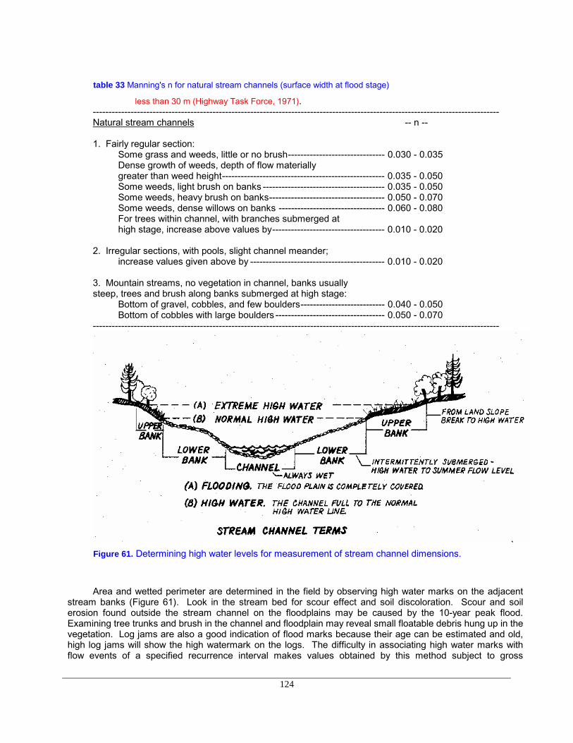
124

table 33 Manning's n for natural stream channels (surface width at flood stage)

less than 30 m (Highway Task Force, 1971).---------------------------------------------------------------------------------------------------------------------------------Natural stream channels -- n --

1. Fairly regular section:Some grass and weeds, little or no brush------------------------------- 0.030 - 0.035Dense growth of weeds, depth of flow materiallygreater than weed height---------------------------------------------------- 0.035 - 0.050Some weeds, light brush on banks --------------------------------------- 0.035 - 0.050Some weeds, heavy brush on banks------------------------------------- 0.050 - 0.070Some weeds, dense willows on banks ---------------------------------- 0.060 - 0.080For trees within channel, with branches submerged athigh stage, increase above values by------------------------------------ 0.010 - 0.020

2. Irregular sections, with pools, slight channel meander;increase values given above by ------------------------------------------- 0.010 - 0.020

3. Mountain streams, no vegetation in channel, banks usuallysteep, trees and brush along banks submerged at high stage:

Bottom of gravel, cobbles, and few boulders--------------------------- 0.040 - 0.050Bottom of cobbles with large boulders ----------------------------------- 0.050 - 0.070

---------------------------------------------------------------------------------------------------------------------------------

Figure 61. Determining high water levels for measurement of stream channel dimensions.

Area and wetted perimeter are determined in the field by observing high water marks on the adjacentstream banks (Figure 61). Look in the stream bed for scour effect and soil discoloration. Scour and soilerosion found outside the stream channel on the floodplains may be caused by the 10-year peak flood.Examining tree trunks and brush in the channel and floodplain may reveal small floatable debris hung up in thevegetation. Log jams are also a good indication of flood marks because their age can be estimated and old,high log jams will show the high watermark on the logs. The difficulty in associating high water marks withflow events of a specified recurrence interval makes values obtained by this method subject to gross

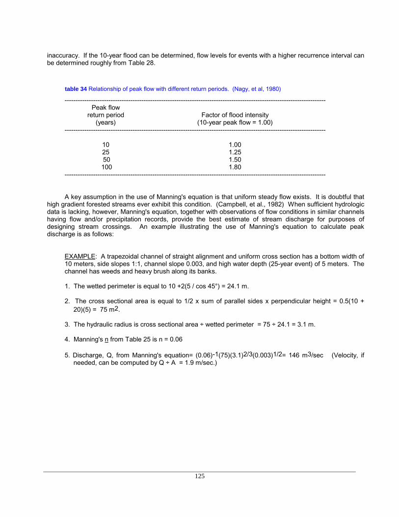
125

inaccuracy. If the 10-year flood can be determined, flow levels for events with a higher recurrence interval canbe determined roughly from Table 28.

table 34 Relationship of peak flow with different return periods. (Nagy, et al, 1980)

-----------------------------------------------------------------------------------------------------------------------Peak flow

return period Factor of flood intensity(years) (10-year peak flow = 1.00)

-----------------------------------------------------------------------------------------------------------------------

10 1.0025 1.25 50 1.50 100 1.80

-----------------------------------------------------------------------------------------------------------------------

A key assumption in the use of Manning's equation is that uniform steady flow exists. It is doubtful thathigh gradient forested streams ever exhibit this condition. (Campbell, et al., 1982) When sufficient hydrologicdata is lacking, however, Manning's equation, together with observations of flow conditions in similar channelshaving flow and/or precipitation records, provide the best estimate of stream discharge for purposes ofdesigning stream crossings. An example illustrating the use of Manning's equation to calculate peakdischarge is as follows:

EXAMPLE: A trapezoidal channel of straight alignment and uniform cross section has a bottom width of10 meters, side slopes 1:1, channel slope 0.003, and high water depth (25-year event) of 5 meters. Thechannel has weeds and heavy brush along its banks.

1. The wetted perimeter is equal to 10 +2(5 / cos 45°) = 24.1 m.

2. The cross sectional area is equal to 1/2 x sum of parallel sides x perpendicular height = 0.5(10 +20)(5) = 75 m2.

3. The hydraulic radius is cross sectional area ÷ wetted perimeter = 75 ÷ 24.1 = 3.1 m.

4. Manning's n from Table 25 is n = 0.06

5. Discharge, Q, from Manning's equation= (0.06)-1(75)(3.1)2/3(0.003)1/2= 146 m3/sec (Velocity, ifneeded, can be computed by Q ÷ A = 1.9 m/sec.)

126

4.3 Channel Crossings

4.3.1 Location of Channel Crossings

Channel crossings require careful design and construction. Functionally, they must (1) allow forpassage of the maximum amount of water which can reasonably be expected to occur within the lifetime ofthe structure and (2) not degrade water quality or endanger the structure itself or any downstream structures.It should be pointed out that most road failures are related to inadequate water passage structures and filldesign and placement as well as poor construction practices in such locations.

Accelerated erosion brought about by failure of channel crossing structures can be caused by:

1 Inadequate design to handle peak flow and debris. Water will back up behind structure, sat- 1uratingthe fill and creating added hydrostatic pressure. Water will overflow the structure and the fill may bewashed out.

2. Inadequate outlet design. By constricting flow through a small area, water velocity (alongwith its erosive power) will increase. Outlets need to be properly designed in order towithstand high flow velocities and thus avoid excessive downstream erosion and eventualroad failure.

3. Poor location of crossing. Crossings need to be located along relatively stable stretches where streambottoms and banks exhibit little signs of excessive erosion or deposition. Meandering and/or multiplechannels often indicate unstable conditions. If there is no choice but to use a poor location, carefulconsideration of the type of crossing selected, along with bank and stream bottom stabilization andprotection measures, should be given.

There are three generally accepted methods used to cross channels on low volume roads--bridges,fords, and culverts. The selection is based on traffic volume and characteristics, site conditions(hydrologic/hydraulic conditions of channel), and management needs such as occasional closure, continuoususe, safety considerations, resource impact (fish, wildlife, sediment). Factors to consider when selecting acrossing type are listed as follows:

1. Bridges: high traffic volume, large and variable water volume, high debris potential, sensitive channelbottom and banks, significant fish resource, large elevation difference between channel and road grade

2. Culvert: Medium to low water volume, medium to low debris potential, fish resource not significant,elevation difference between channel and road grade less than 10 meters, high traffic volume

3. Ford: low to intermittent water flow, high debris potential, no fish resource, road grade can be broughtdown to channel bottom, low traffic volume

All three channel crossing types require a careful analysis of both vertical and horizontal alignment. Inparticular, careful analysis of curve widening requirements is imperative in relation to the specified criticalvehicle. Channel crossings are fixed structures where the road way width cannot be temporarily widened.Road width, curvature, approach, and exit tangents govern the vehicle dimensions which can pass thecrossing.

Except for bridge locations, roads should climb away from channel crossings in both directions whereverpractical so high water will not flow along the road surface. This is particularly true for ford installations.

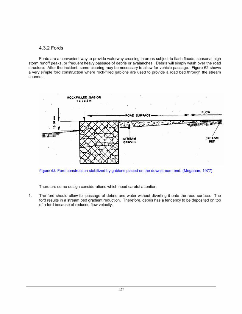
127

4.3.2 Fords

Fords are a convenient way to provide waterway crossing in areas subject to flash floods, seasonal highstorm runoff peaks, or frequent heavy passage of debris or avalanches. Debris will simply wash over the roadstructure. After the incident, some clearing may be necessary to allow for vehicle passage. Figure 62 showsa very simple ford construction where rock-filled gabions are used to provide a road bed through the streamchannel.

Figure 62. Ford construction stabilized by gabions placed on the downstream end. (Megahan, 1977)

There are some design considerations which need careful attention:

1. The ford should allow for passage of debris and water without diverting it onto the road surface. Theford results in a stream bed gradient reduction. Therefore, debris has a tendency to be deposited on topof a ford because of reduced flow velocity.

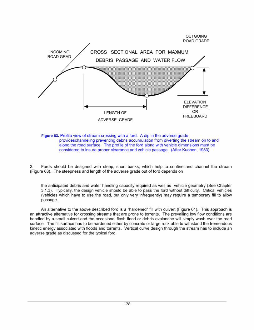
128

INCOMING ROAD GRAD

OUTGOING ROAD GRADE

LENGTH OF

ADVERSE GRADE

ELEVATION DIFFERENCE

OR FREEBOARD

CROSS SECTIONAL AREA FOR MAXIMUM

DEBRIS PASSAGE AND WATER FLOW

Figure 63. Profile view of stream crossing with a ford. A dip in the adverse gradeprovideschanneling preventing debris accumulation from diverting the stream on to andalong the road surface. The profile of the ford along with vehicle dimensions must beconsidered to insure proper clearance and vehicle passage. (After Kuonen, 1983)

2. Fords should be designed with steep, short banks, which help to confine and channel the stream(Figure 63). The steepness and length of the adverse grade out of ford depends on

the anticipated debris and water handling capacity required as well as vehicle geometry (See Chapter3.1.3). Typically, the design vehicle should be able to pass the ford without difficulty. Critical vehicles(vehicles which have to use the road, but only very infrequently) may require a temporary fill to allowpassage.

An alternative to the above described ford is a "hardened" fill with culvert (Figure 64). This approach isan attractive alternative for crossing streams that are prone to torrents. The prevailing low flow conditions arehandled by a small culvert and the occasional flash flood or debris avalanche will simply wash over the roadsurface. The fill surface has to be hardened either by concrete or large rock able to withstand the tremendouskinetic energy associated with floods and torrents. Vertical curve design through the stream has to include anadverse grade as discussed for the typical ford.

129

Figure 64. Hardened fill stream crossings provide an attractive alternative for streams prone totorrents or debris avalanches (Amimoto, 1978).

4.3.3 Culverts

Culverts are by far the most commonly used channel crossing structure used on forest roads. Culverttypes normally used, and the conditions under which they are used, are as follows:

Corrugated metal pipe (CMP) ....................All conditions except those noted below

CMP with paved invert ................................Water carries sediments erosive to metal

CM pipe-arch ..............................................Low fills; limited head room

Multi-plate....................................................Large sizes (greater than 1.8 meters)

Reinforced concrete pipe ...........................Corrosive soil or water, as salt water; short(RCP) haul from plant; unloading and placing equipment available

130

Reinforced concrete box .............................Extra large waterway; migratory fish way

Although more expensive than round culverts, pipe-arch or plate arch types are preferred over ordinaryround pipes. Pipe-arch culverts, besides having a more efficient opening per unit area than round pipe for agiven discharge, will collect bottom sediments over time when it is installed slightly below the stream grade.They also require lower fills. However, during periods of low flow, water in pipes with this shape may bespread so thin across the bottom that fish passage is impossible. A plate-arch set in concrete footings is themost desirable type from a fish passage standpoint since it has no bottom. The stream can remain virtuallyuntouched if care is exercised during its installation. (Yee and Roelofs, 1980)

Regardless of the type of culvert, they should all conform to proper design standards with regards toalignment with the channel, capacity, debris control, and energy dissipation. They should all perform thefollowing functions:

1. The culvert with its appurtenant entrance and outlet structures should efficiently discharge water,bedload, and floating debris at all stages of flow.

2. It should cause no direct or indirect property damage.

3. It should provide adequate transport of water, debris, and sediment without drastic changes in flowpatterns above or below the structure.

4. It should be designed so that future channel and highway improvements can be made without muchdifficulty.

5. It should be designed to function properly after fill has settled.

6. It should not cause objectionable stagnant pools in which mosquitoes could breed.

7. It should be designed to accommodate increased runoff occasioned by anticipated land development.

8. It should be economical to build, hydraulically adequate to handle design discharge, structurally durable,and easy to maintain.

9. It should be designed to avoid excessive ponding at the entrance, which may cause property damage,accumulation of sediment, culvert clogging, saturation of fills, or detrimental upstream deposits ofdebris.

10. Entrance structures should be designed to screen out material which will not pass through the culvert,reduce entrance losses to a minimum, make use of velocity of approach insofar as practical, and by useof transitions and increased slopes, as necessary, facilitate channel flow entering the culvert.

11. The outlet design should be effective in re-establishing tolerable non-erosive channel flow within theright-of-way or within a reasonably short distance below the culvert, and should resist undercutting andwashout.

12. Energy dissipators should be simple, easy to build, economical and reasonably self-cleaning duringperiods of low flow.

131

Figure 65. Possible culvert alignments to minimize channel scouring. (USDA, Forest Service, 1971)

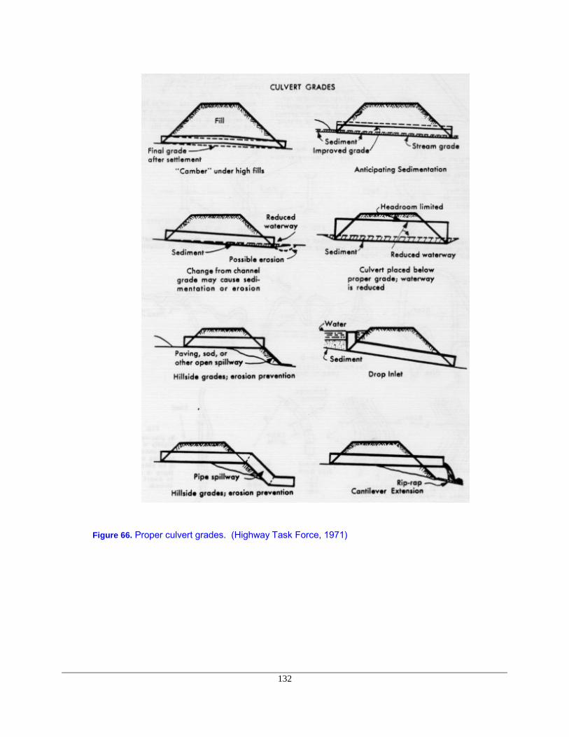
132

Figure 66. Proper culvert grades. (Highway Task Force, 1971)

133

13. Alignment should be such that water enters and exits the culvert directly. Any abrupt change in directionat either end will retard flow and cause ponding, erosion, or a buildup of debris at the culvert entrance.All of these conditions could lead to failure. (See Figure 65 for suggested culvert-channel alignmentconfigurations and Figure 66 for suggested culvert grades. In practice, culvert grade lines generallycoincide with the average streambed above and below the culvert.)

If there are existing roads in the watershed, examination of the performance of existing culverts oftenserves as the best guide to determining the type, size, and accompanying inlet/outlet improvements neededfor the proposed stream crossing. For estimating streamflow on many forest watersheds, existing culvertinstallations may be used as "control sections". Flow can be calculated as the product of water velocity (V)and cross-sectional area (A):

Q = A * V.

Cross-sectional area of water flowing in a round culvert is difficult to measure, however a rough estimatecan be calculated from the following equation:

A = [(πr2ß) /180] - (r2-rd) sinß

where r = culvert radius

d = measured depth of flow

ß = angle (°) between radial lines to the bottom of the culvert and to the water surface (Figure 62)

= cos-1 [(r-d) / r].

Figure 67. Definition sketch of variables used in flow calculations.

Velocity can be calculated using Manning's equation:

V = Q / A =( n-1)(R2/3)(S1/2)

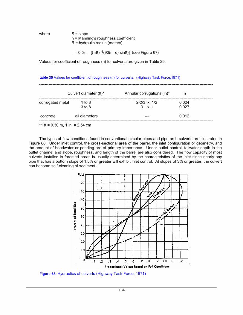
134

where S = slopen = Manning's roughness coefficientR = hydraulic radius (meters)

= 0.5r - [(πß)-1(90(r - d) sinß)] (see Figure 67)

Values for coefficient of roughness (n) for culverts are given in Table 29.

table 35 Values for coefficient of roughness (n) for culverts. (Highway Task Force,1971)

----------------------------------------------------------------------------------------------------------------------------------

Culvert diameter (ft)* Annular corrugations (in)* n----------------------------------------------------------------------------------------------------------------------------------corrugated metal 1 to 8 2-2/3 x 1/2 0.024

3 to 8 3 x 1 0.027

concrete all diameters --- 0.012----------------------------------------------------------------------------------------------------------------------------------*1 ft = 0.30 m, 1 in. = 2.54 cm

The types of flow conditions found in conventional circular pipes and pipe-arch culverts are illustrated inFigure 68. Under inlet control, the cross-sectional area of the barrel, the inlet configuration or geometry, andthe amount of headwater or ponding are of primary importance. Under outlet control, tailwater depth in theoutlet channel and slope, roughness, and length of the barrel are also considered. The flow capacity of mostculverts installed in forested areas is usually determined by the characteristics of the inlet since nearly anypipe that has a bottom slope of 1.5% or greater will exhibit inlet control. At slopes of 3% or greater, the culvertcan become self-cleaning of sediment.

Figure 68. Hydraulics of culverts (Highway Task Force, 1971)

135

Once the design peak discharge has been determined by one of the methods discussed above, the sizeof pipe required to handle the discharge can be determined from available equations, charts, tables,nomographs, etc., such as the ones presented in Figures 70, 71, 72, 73 and 74. Figure 69 provides anexample of a work sheet which can be used for diameter and flow capacity calculations. If outlet control isindicated (for example, in a low gradient reach where "backwater effects" may be created at the outlet end),the reader is referred to Handbook of Steel Drainage and Highway Construction Products (1971) or CircularNo. 5 published by the U. S. Department of Commerce (1963). Outlet control conditions are shown in Figure74 for a corrugated metal pipe.

It is important to keep in mind that in addition to discharge from areas upstream of the installation, theculvert must be able to handle accumulated water from roadside ditches recalling that roadside ditches onroads lower on the slope intercept more subsurface water than those on roads higher on the slope. Suddensurges from rapid snowmelt (if applicable) must also be allowed for. Organic debris and bedload sedimentscan plug a culvert and can greatly reduce culvert efficiency. For these reasons, an "oversized" culvert designmay be indicated.

Inlet characteristics can greatly influence flow efficiency through the culvert. The end either (1) projectsbeyond the fill, (2) is flush with a headwall, or (3) is supplemented with a manufactured mitered steel endsection. Inlets with headwalls are generally the most efficient followed by culverts with mitered inlets andfinally culverts with projecting entrances. When headwater depths are 1 to 2 times greater than culvertdiameter, culverts with headwalls have an increase in flow capacity of approximately 11 and 15%,respectively, over culverts with projecting entrances.

Procedure for Selection of Culvert Size

Note: Culvert design sheets, similar to Figure 69 should be used to record design data.

Step 1: List given data: a. Design discharge Q, in m3/sec.

b. Approximate length of culvert, in meters.

c. Allowable headwater depth, in meters. Headwater depth is defined as the vertical distance from theculvert invert (flow line) at the entrance to the water surface elevation permissible in the approachchannel upstream from the culvert.

d. Type of culvert, including barrel material, barrel cross-sectional shape and entrance type.

e. Slope of culvert. (If grade is given in percent, convert to slope in meters per meter).

f. Allowable outlet velocity (if scour or fish passage is a concern).

g. Convert metric units to english units for use with the nomographs.

Volume flow Q(m3/sec) to Q(cfs) : 1 m3/sec = 35.2 cfs (cubic ft/sec). Multiply Q(m3/sec) by 35.2to get Q(cfs)

Length, Diameter (meter): 1 meter = 3.3 ft.; 1 cm = 0.4 inches. Multiply (cm) by 0.4 to get(inches). Multiply (meter) by 3.3 to get (feet)

Step 2: Determine a trial size culvert:

136

a. Refer to the inlet control nomograph for the culvert type selected.

b. Using an HW / D (Headwater depth/Diameter)) of approximately 1.5 and the scale for the entrancetype to be used, find a trial size culvert by following the instructions for use of the nomographs. If alesser or greater relative headwater depth should be needed, another value of HW/D may be used.

c. If the trial size for the culvert is obviously too large because of limited height of embankment or sizeavailability, try different HW/D values or multiple culverts by dividing the discharge equally for thenumber of culverts used. Raising the embankment height or using a pipe arch and box culvert whichallow for lower fill heights is more efficient hydraulically than using the multiple culvert approach.Given equal end areas, a pipe arch will handle a larger flow than two round culverts. Selection shouldbe based on an economic analysis.

Step 3: Find headwater (HW) depth for the trial size culvert:

a. Determine and record HW depth by use of the appropriate inlet control nomograph. Tailwater (TW)conditions are to be neglected in this determination. HW in this case is found by simply multiplyingHW/D (obtained from the nomograph) by D.

Step 4: Check outlet velocities for size selected:

a. If inlet control governs, outlet velocity can be assumed to equal normal velocity in open-channel flowas computed by Manning's equation for the barrel size, roughness, and slope of culvert selected.

Note: In computing outlet velocities, charts and tables such as those provided by U.S. Army Corp ofEngineers, Bureau of Reclamation, and Department of Commerce are helpful (see LiteratureCited).

Step 5: Try a culvert of another type or shape and determine size and HW by the procedure above.

Step 6: Record final selection of culvert with size, type, outlet velocity, required HW and economicjustification. A good historical record of culvert design, installation, and performanceobservations can be a valuable tool in planning and designing future installations.

Instructions for Using Inlet Control Nomographs

1. To determine headwater (HW):

a. Connect with a straight edge the given culvert diameter or height (D) and the discharge Q, or Q/B forbox culverts; mark intersection of straightedge on HW/D scale mark (1).

b. If HW / D scale mark (1) represents entrance type used, read HW / D on scale (1). If some otherentrance type is used, extend the point of intersection found in (a) horizontally to scale (2) or (3) andread HW/D.

c. Compute HW by multiplying HW / D by D.

2. To determine culvert size:

a. Given an HW / D value, locate HW / D on scale for appropriate entrance type. If scale (2) or (3) isused, extend HW / D point horizontally to scale (1).

137

b. Connect point on HW / D scale (1) as found in (a) above to given discharge and read diameter ofculvert required.

3. To determine discharge (Q):

a. Given HW and D, locate HW / D on scale for appropriate entrance type. Continue as in 2a.

b. Connect point on HW / D scale (1) as found in (a) above, the size of culvert on the left scale, andread Q or Q/B on the discharge scale.

c. If Q/B is read in (b) multiply by B to find Q.

Good installation practices are essential for proper functioning of culverts, regardless of the materialused in the construction of the culvert (Figure 75). Flexible pipe such as aluminum, steel, or polyethylene,requires good side support and compaction, particularly in the larger sizes. It is recommended that the roadbe constructed to grade or at least a meter above the top of the pipe, the fill left to settle and then excavated toform the required trench.

The foundation dictates if bedding is needed or not. Proper foundation maintains the conduit on auniform grade. Most times, the culvert can be laid without bedding, however, a few centimeters of beddinghelps in installation of the culvert. When bedding is required, the depth should be 8 cm if the foundationmaterial is soil and 30 cm if it is rock.

Backfilling is the most important aspect of culvert installation. Ten percent of the loading is taken by thepipe and 90 percent is taken by the material surrounding the pipe if backfilling is done correctly. Backfillmaterial should consist of earth, sand, gravel, rock or combinations thereof, free of humus, organic matter,vegetative matter, frozen material, clods, sticks and debris and containing no stones greater than 8 cm (3 in)in diameter. It should be placed in layers of no greater than 15 cm (6 in) and compacted up to 95% of Proctordensity at or near the optimum moisture content for the material.

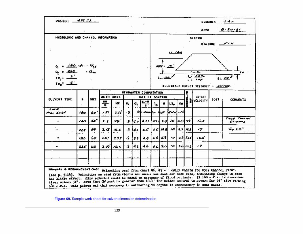
139

Figure 69. Sample work sheet for culvert dimension determination

140

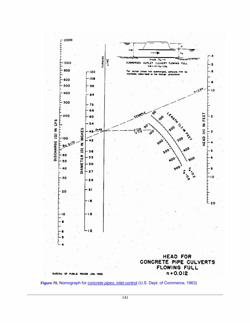
141

Figure 70. Nomograph for concrete pipes, inlet control (U.S. Dept. of Commerce, 1963)

142

Figure 71. Nomograph for corrugated metal pipe (CMP), inlet control. (U.S. Dept. ofCommerce,1963).

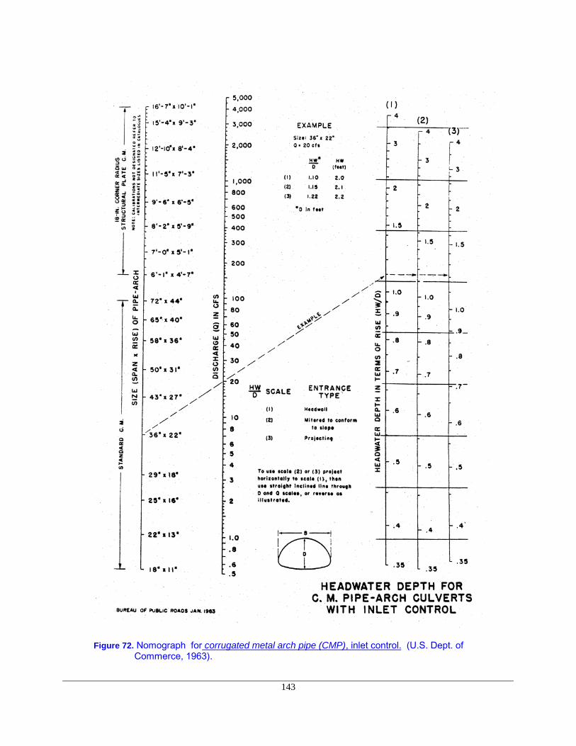
143

Figure 72. Nomograph for corrugated metal arch pipe (CMP), inlet control. (U.S. Dept. ofCommerce, 1963).

144

Figure 73. Nomograph for box - culvert, inlet control. (U.S. Dept. of Commerce, 1963).

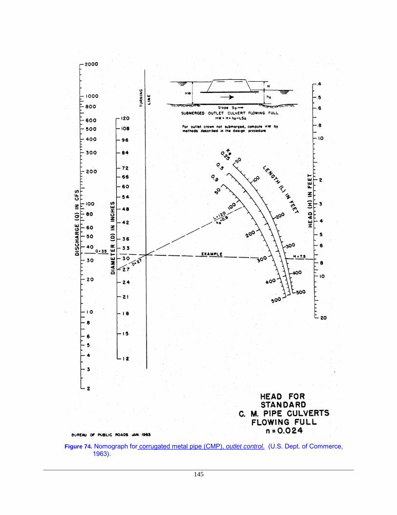
145

Figure 74. Nomograph for corrugated metal pipe (CMP), outlet control. (U.S. Dept. of Commerce,1963).

146

Figure 75. Proper pipe foundation and bedding (1 ft. = 30 cm). (USDA, Forest Service, 1971)

147

4.3.4 Debris Control Structures

A critical factor in the assessment of channel crossing design and structural capacity is its allowance forhandling or passing debris. Past experience has shown that channel crossings have failed not because ofinadequate design to handle unanticipated water flows, but because of inadequate allowances for floatabledebris which eventually blocked water passage through the culvert. Therefore, each channel crossing has tobe analyzed for its debris handing capacity.

When upstream organic debris poses an immediate threat to the integrity of the culvert, severalalternatives may be considered.

1. Cleaning the stream of floatable debris is risky and expensive. Since many of the hydrauliccharacteristics of the channel are influenced by the size and placement of debris, its removal must becarried out only after a trained specialist, preferably a hydrologist, has made a site-specific evaluation ofchannel stability factors.

2. Various types of mechanical structures (Figures 76, 77 and 78) can be placed above the inlet to catchany debris that may become entrained.

3. A bridge may be substituted in place of a culvert.

FRONT VIEW

TOP VIEW

Figure 76. Debris control structure--cribbing made of timber.

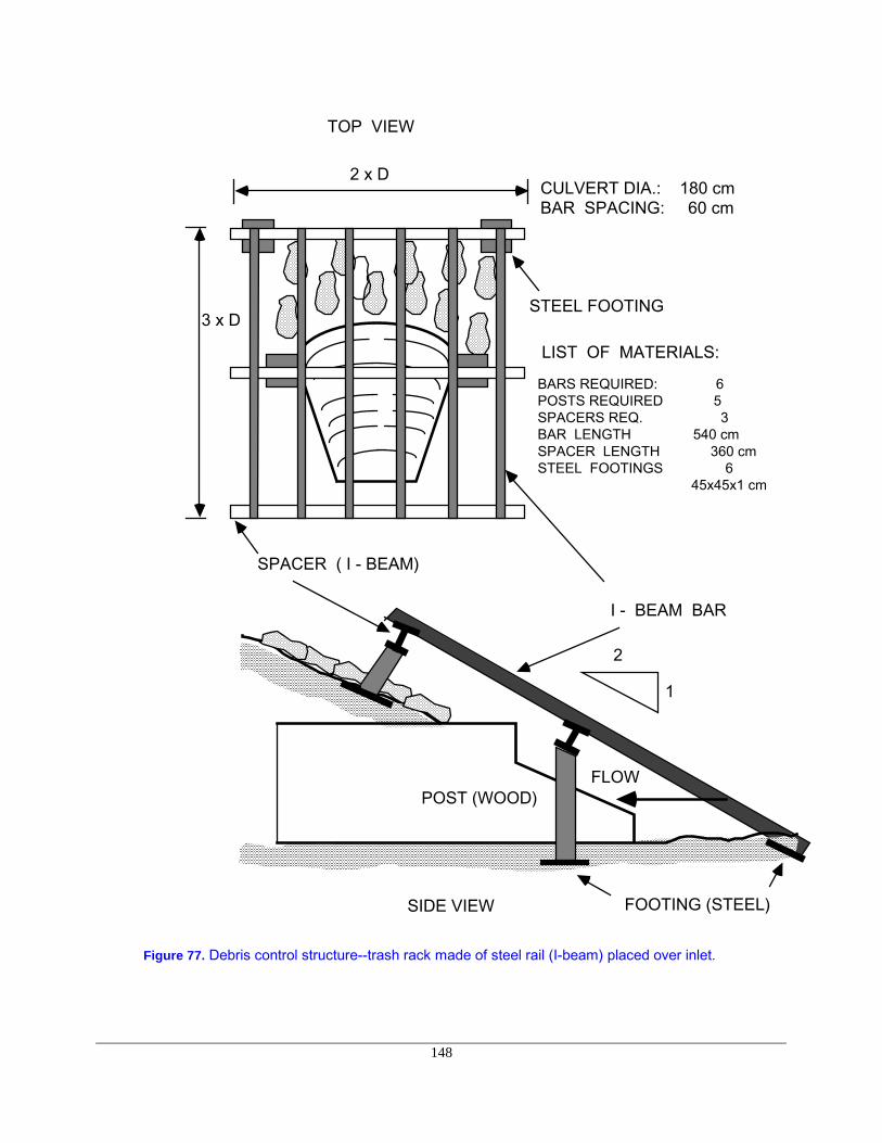
148

I - BEAM BAR

STEEL FOOTING

POST (WOOD)

FOOTING (STEEL)

SPACER ( I - BEAM)

3 x D

2 x D

TOP VIEW

SIDE VIEW

LIST OF MATERIALS:

BARS REQUIRED: 6 POSTS REQUIRED 5 SPACERS REQ. 3 BAR LENGTH 540 cm SPACER LENGTH 360 cm STEEL FOOTINGS 6 45x45x1 cm

2

1

FLOW

CULVERT DIA.: 180 cm BAR SPACING: 60 cm

Figure 77. Debris control structure--trash rack made of steel rail (I-beam) placed over inlet.

149

D

DD D

1/2 D

2 D

D at Inlet 2D at Outlet

CLAY OR OTHER SUITABLE MATERIAL

FOR SEEPAGE CUT OFF UNDER BOTH ENDS

GRANULAR BEDDING MATERIAL

1/2 D

IN LET / OUTLET PROTECTIONCULVERT

Rip - Rap

Figure 78. Inlet and outlet protection of culvert with rip-rap. Rocks used should typically weigh 20 kgor more and approximately 50 percent of the rocks should be larger than 0.1 m3 involume. Rocks can also be replaced with cemented sand layer (1 part cement, 4 partssand).

Under high fills, inlets can be provided with upstream protection by rock riprap up to the high water mark(Figure 78). Cambering may also be necessary to ensure the proper grade after fill settlement.

150

4.3.5 Bridges

Bridges often represent the preferred channel crossing alternative in areas where aquatic resources areextremely sensitive to disturbance. However, poor location of footings, foundations, or abutments can causechannel scour and contribute to debris blockage.

Bridges have been designed using a variety of structural materials for substructure and superstructure.Selection of a bridge type for a specific site should take into consideration the functional requirements of thesite, economics of construction at that site, live load requirements, foundation conditions, maintenanceevaluations, and expertise of project engineer.

Some arbitrary rules for judging the minimum desirable horizontal and vertical stream clearances instreams not subject to navigation may be established for a specific area based on judgment and experience.In general, vertical clearances should be greater than or equal to 1.5 meters (5 feet) above the 50-year floodlevel plus 0.02 times the horizontal distance between piers. Horizontal clearance between piers or supports inforested lands or crossings below forested lands should not be less than 85 percent of the anticipated treeheight in the forested lands or the lateral width of the 50-year flood. (US Environmental Protection Agency,1975)

Of course, longer bridge spans will require careful economic evaluations since higher superstructurecosts are often involved. Subaqueous foundations are expensive and involve a high degree of skill in theconstruction of protective cofferdams, seal placement and cofferdam dewatering. In addition to threats towater quality that can occur from a lost cofferdam, time and money losses will be significant. Subaqueousfoundations often limit the season of construction relative to water level and relative to fish spawning activity.Thus, construction timing must be rigidly controlled.

It is suggested that the maximum use be made of precast or prefabricated superstructure units since theremoteness of many mountain roads economically precludes bridge construction with unassembled materialsthat must be transported over great distances. However, the use of such materials may be limited by thecapability to transport the units over narrow, high curvature roads to the site, or by the horizontal geometry ofthe bridge itself.

Another alternative is the use of locally available timber for log stringer bridges. An excellent referencefor the design and construction of single lane log bridges is Log Bridge Construction Handbook, by M. M.Nagy, et al., and is published by the Forest Engineering Research Institute of Canada. The reader is referredto this publication for more detailed discussions of these topics.

151

4.4 Road Surface Drainage

4.4.1 Surface Sloping

Reducing the erosive power of water can achieved by reducing its velocity. If, for practical reasons,water velocity cannot be reduced, surfaces must be hardened or protected as much as possible to minimizeerosion from high velocity flows. Road surface drainage attempts to remove the surface water before itaccelerates to erosive velocities and/or infiltrates into the road prism destroying soil strength by increasingpore water pressures. This is especially true for unpaved, gravel, or dirt roads.

Water moves across the road surface laterally or longitudinally. Lateral drainage is achieved bycrowning or by in- or out-sloping of road surfaces (Figure 79). Longitudinal water movement is intercepted bydips or cross drains. These drainage features become important on steep grades or on unpaved roads whereruts may channel water longitudinally on the road surface.

OUTSLOPED

3 - 5 %

Typical for temporary roads with dirt surface ( no ballast )

Water flows onto protected and / or stable fill areas.

IN SLOPED

DITCH LINE

BALLAST

3 - 5 %

Typical for permanent roads; with or without ballast or ditch line

CROWNED SURFACE3 - 10 %

Fastest water removal. Requires water control on both sides.

DITCH LINE

Figure 79. Road cross section grading patterns used to control surface drainage.

152

table 36 Effect of in-sloping on sediment yield of a graveled, heavily used road segment with a 10 % downgrade for different cross slopes*

------------------------------------------------------------------------------------------------------------------------------Transverse Sediment Delivery

grade tonnes/ha/year------------------------------------------------------------------------------------------------------------------------------

conventional0 - 2 % 970

5 % 4009 % 30012 % 260

------------------------------------------------------------------------------------------------------------------------------*4 meter wide road surface 4 - 16 trucks/day 3900 mm annual precipitation

Sloping or crowning significantly reduces sediment delivery from road surfaces. A study by Reid (1981)showed a reduction in sediment delivery by increasing the transverse road surface grade. In this particularcase the road surfaces insloped from 5 to 12 percent were compared with conventionally constructed roadsurfaces at grades of 0 to 2 percent. Sediment yield was reduced by a factor of 3.0 to 4.5 when compared toa conventionally sloped road (Table 30).

Outsloping is achieved by grading the surface at 3 to 5 percent cross slope toward the downhill side ofthe road. Outsloped roads are simple to build and to maintain. Disadvantages of outsloping include trafficsafety concerns and lack of water discharge control. When surfaces become slippery (i.e., snow or ice cover,or when silty or clayey surfaces become wet), vehicles may lose traction and slide toward the downhill edge.Outsloping should only be used under conditions where run-off can be directed onto stable areas. If terrain isless than 20 percent slope and the road gradient is less than 4 percent, outsloping is not an effective way ofwater removal.

Temporary roads or roads with very light traffic can be outsloped where side slopes do not exceed 40percent. For safety reasons, when side slopes exceed 40 percent, traffic restrictions should be in force duringinclement weather. When outsloping is used for surface drainage, cross drains or dips should be installed onthe road surface (Figure 75). Spacing will depend on soil type, road surface and road grade.

Insloping is used where a more reliable drainage system is required such as on permanent roads, roadswith high anticipated traffic volumes and/or loads, or in areas with sensitive soils or severe climatic conditions.Insloping is achieved by grading the road surface towards the uphill side of the road at a 3 to 5 percent grade.Water draining from insloped road surfaces is collected and carried along the inside of the road either on theroad surface itself or more commonly in a ditch line. The ditch line can be omitted from the road template,thereby reducing the overall road width. This may be desirable in steep terrain in order to reduce excavation(see also Section 3.2). However, this option must be weighed against potential drainage problems along theuphill side of the road. Dips, cross drains, or culverts must be installed and maintained to remove water fromthe road prism.

Crowned surfaces provide the fastest water removal since the distance water has to travel is cut in half.The crowned surface slopes at 3 to 10 percent from either side of the road centerline. Crowned surfaces andany associated cross drains or dips are difficult to maintain. Water has to be controlled on both sides of theroad through a ditch line and stable areas have to be provided for runoff water. Ballast thickness is typicallythe largest in the center in order to achieve the correct crown shape.

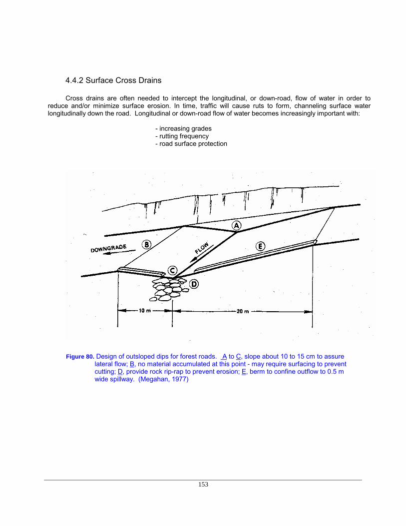
153

4.4.2 Surface Cross Drains

Cross drains are often needed to intercept the longitudinal, or down-road, flow of water in order toreduce and/or minimize surface erosion. In time, traffic will cause ruts to form, channeling surface waterlongitudinally down the road. Longitudinal or down-road flow of water becomes increasingly important with:

- increasing grades- rutting frequency- road surface protection

Figure 80. Design of outsloped dips for forest roads. A to C, slope about 10 to 15 cm to assurelateral flow; B, no material accumulated at this point - may require surfacing to preventcutting; D, provide rock rip-rap to prevent erosion; E, berm to confine outflow to 0.5 mwide spillway. (Megahan, 1977)

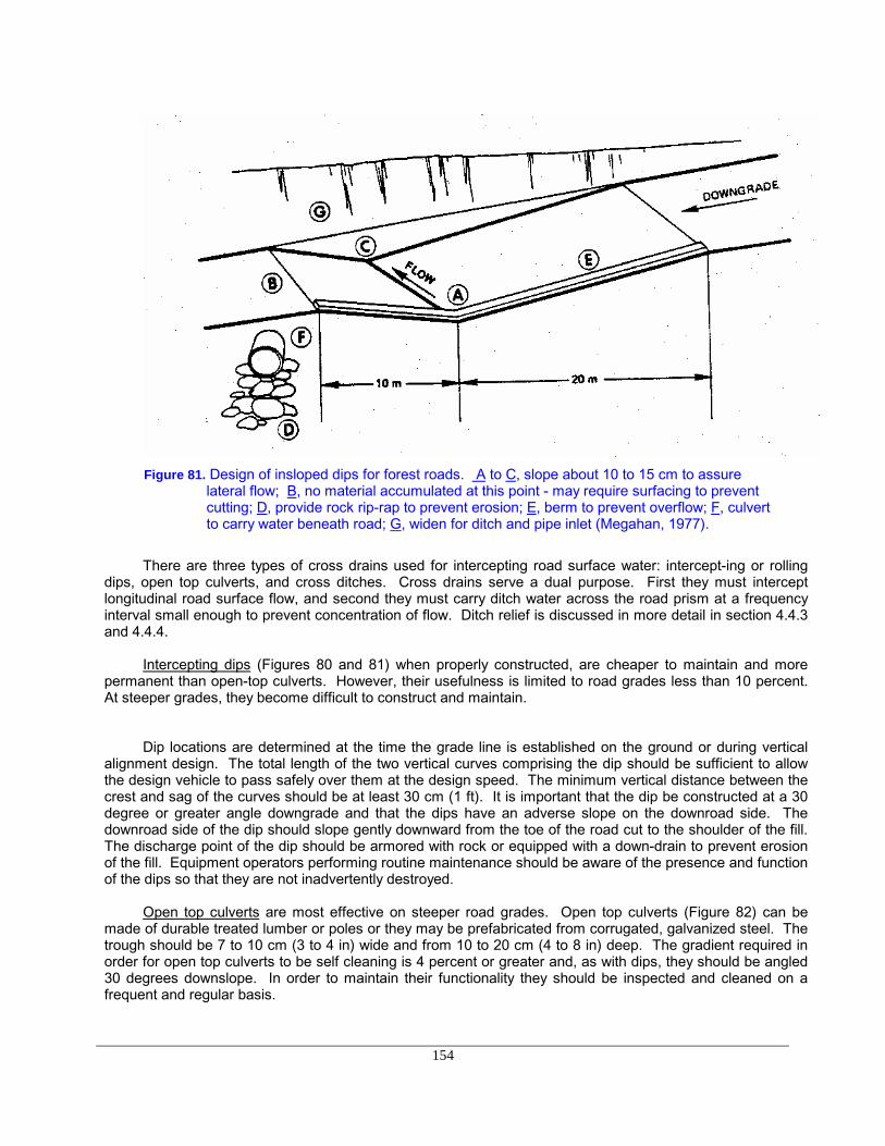
154

Figure 81. Design of insloped dips for forest roads. A to C, slope about 10 to 15 cm to assurelateral flow; B, no material accumulated at this point - may require surfacing to preventcutting; D, provide rock rip-rap to prevent erosion; E, berm to prevent overflow; F, culvertto carry water beneath road; G, widen for ditch and pipe inlet (Megahan, 1977).

There are three types of cross drains used for intercepting road surface water: intercept-ing or rollingdips, open top culverts, and cross ditches. Cross drains serve a dual purpose. First they must interceptlongitudinal road surface flow, and second they must carry ditch water across the road prism at a frequencyinterval small enough to prevent concentration of flow. Ditch relief is discussed in more detail in section 4.4.3and 4.4.4.

Intercepting dips (Figures 80 and 81) when properly constructed, are cheaper to maintain and morepermanent than open-top culverts. However, their usefulness is limited to road grades less than 10 percent.At steeper grades, they become difficult to construct and maintain.

Dip locations are determined at the time the grade line is established on the ground or during verticalalignment design. The total length of the two vertical curves comprising the dip should be sufficient to allowthe design vehicle to pass safely over them at the design speed. The minimum vertical distance between thecrest and sag of the curves should be at least 30 cm (1 ft). It is important that the dip be constructed at a 30degree or greater angle downgrade and that the dips have an adverse slope on the downroad side. Thedownroad side of the dip should slope gently downward from the toe of the road cut to the shoulder of the fill.The discharge point of the dip should be armored with rock or equipped with a down-drain to prevent erosionof the fill. Equipment operators performing routine maintenance should be aware of the presence and functionof the dips so that they are not inadvertently destroyed.

Open top culverts are most effective on steeper road grades. Open top culverts (Figure 82) can bemade of durable treated lumber or poles or they may be prefabricated from corrugated, galvanized steel. Thetrough should be 7 to 10 cm (3 to 4 in) wide and from 10 to 20 cm (4 to 8 in) deep. The gradient required inorder for open top culverts to be self cleaning is 4 percent or greater and, as with dips, they should be angled30 degrees downslope. In order to maintain their functionality they should be inspected and cleaned on afrequent and regular basis.

155

Figure 82. Installation of an open-top culvert. Culverts should be slanted at 30 degrees downslope tohelp prevent plugging. Structure can be made of corrugated steel, lumber or other, similarmaterial. (Darrach, et al., 1982)

Figure 83. Cross ditch construction for forest roads with limited or no traffic. Specifications aregeneralized and may be adjusted for gradient and other conditions. A, bank tie-in pointcut 15 to 30 cm into roadbed; B, cross drain berm height 30 to 60 cm above road bed; C,drain outlet 20 to 40 cm into road; D, angle drain 30 to 40 degrees downgrade with roadcenterline; E, height up to 60 cm, F, depth to 45 cm; G, 90 to 120 cm. (Megahan, 1977)

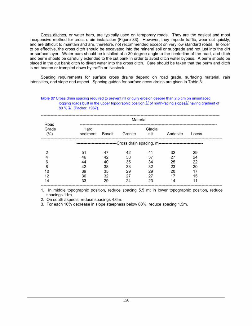
156

Cross ditches, or water bars, are typically used on temporary roads. They are the easiest and mostinexpensive method for cross drain installation (Figure 83). However, they impede traffic, wear out quickly,and are difficult to maintain and are, therefore, not recommended except on very low standard roads. In orderto be effective, the cross ditch should be excavated into the mineral soil or subgrade and not just into the dirtor surface layer. Water bars should be installed at a 30 degree angle to the centerline of the road, and ditchand berm should be carefully extended to the cut bank in order to avoid ditch water bypass. A berm should beplaced in the cut bank ditch to divert water into the cross ditch. Care should be taken that the berm and ditchis not beaten or trampled down by traffic or livestock.

Spacing requirements for surface cross drains depend on road grade, surfacing material, rainintensities, and slope and aspect. Spacing guides for surface cross drains are given in Table 31.

table 37 Cross drain spacing required to prevent rill or gully erosion deeper than 2.5 cm on unsurfacedlogging roads built in the upper topographic position 1/ of north-facing slopes2/ having gradient of80 % 3/ (Packer, 1967).

---------------------------------------------------------------------------------------------------------------------------------Material

Road ---------------------------------------------------------------------------------------------------Grade Hard Glacial(%) sediment Basalt Granite silt Andesite Loess

----------------------------------------------------------------------------------------------------------------------------------- -----------------------------Cross drain spacing, m--------------------------------

2 51 47 42 41 32 29 4 46 42 38 37 27 24 6 44 40 35 34 25 22 8 42 38 33 32 23 2010 39 35 29 29 20 1712 36 32 27 27 17 1514 33 29 24 23 14 11

-----------------------------------------------------------------------------------------------------------------------------------1. In middle topographic position, reduce spacing 5.5 m; in lower topographic position, reduce

spacings 11m.2. On south aspects, reduce spacings 4.6m.3. For each 10% decrease in slope steepness below 80%, reduce spacing 1.5m.

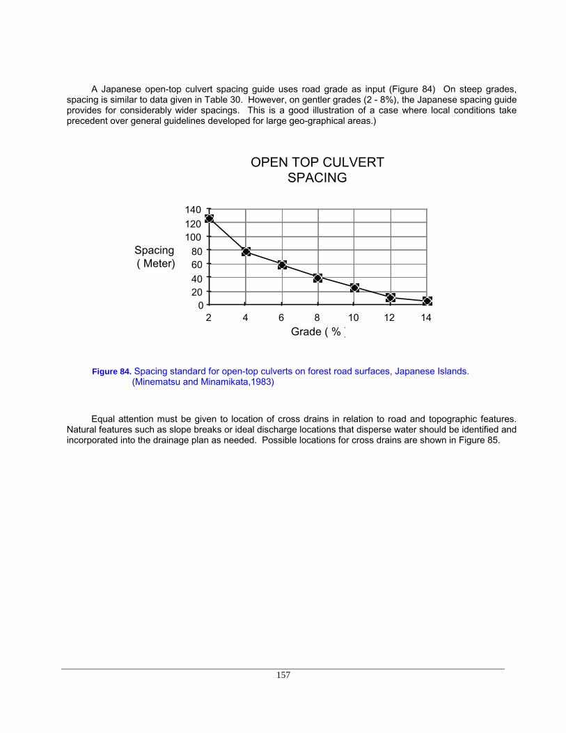
157

A Japanese open-top culvert spacing guide uses road grade as input (Figure 84) On steep grades,spacing is similar to data given in Table 30. However, on gentler grades (2 - 8%), the Japanese spacing guideprovides for considerably wider spacings. This is a good illustration of a case where local conditions takeprecedent over general guidelines developed for large geo-graphical areas.)

020406080

100120140

2 4 6 8 10 12 14

OPEN TOP CULVERTSPACING

Grade ( % )

Spacing( Meter)

Figure 84. Spacing standard for open-top culverts on forest road surfaces, Japanese Islands.(Minematsu and Minamikata,1983)

Equal attention must be given to location of cross drains in relation to road and topographic features.Natural features such as slope breaks or ideal discharge locations that disperse water should be identified andincorporated into the drainage plan as needed. Possible locations for cross drains are shown in Figure 85.

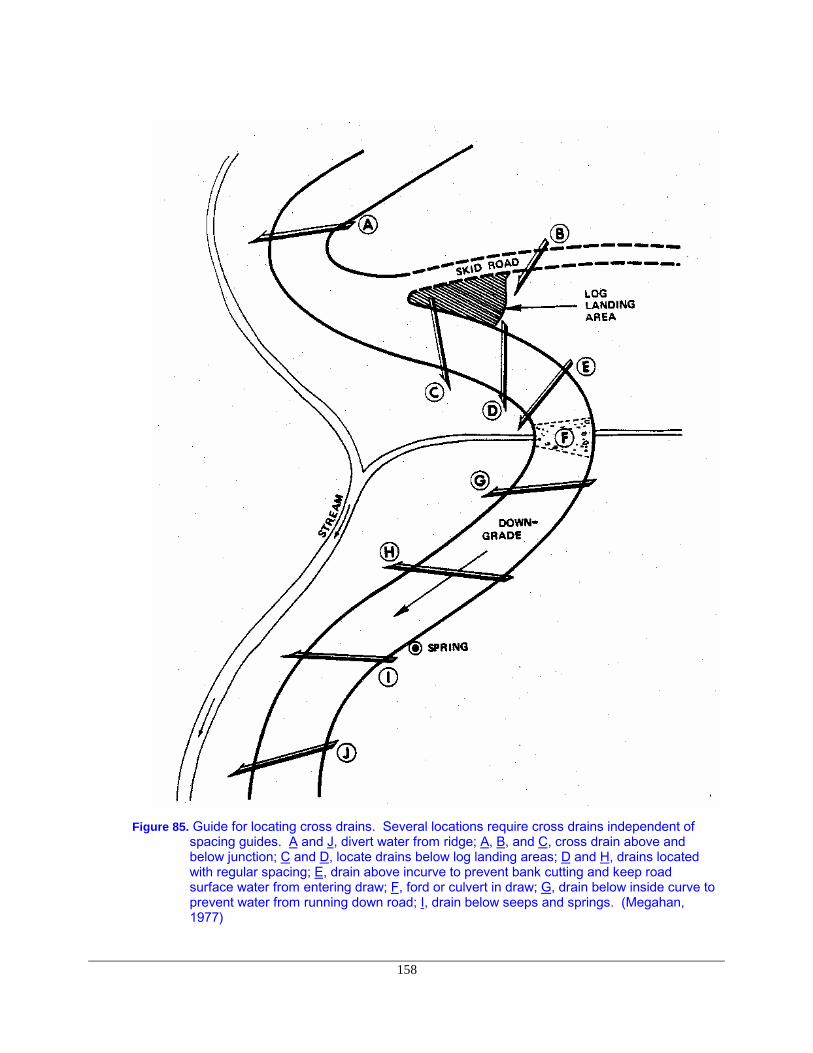
158

Figure 85. Guide for locating cross drains. Several locations require cross drains independent ofspacing guides. A and J, divert water from ridge; A, B, and C, cross drain above andbelow junction; C and D, locate drains below log landing areas; D and H, drains locatedwith regular spacing; E, drain above incurve to prevent bank cutting and keep roadsurface water from entering draw; F, ford or culvert in draw; G, drain below inside curve toprevent water from running down road; I, drain below seeps and springs. (Megahan,1977)

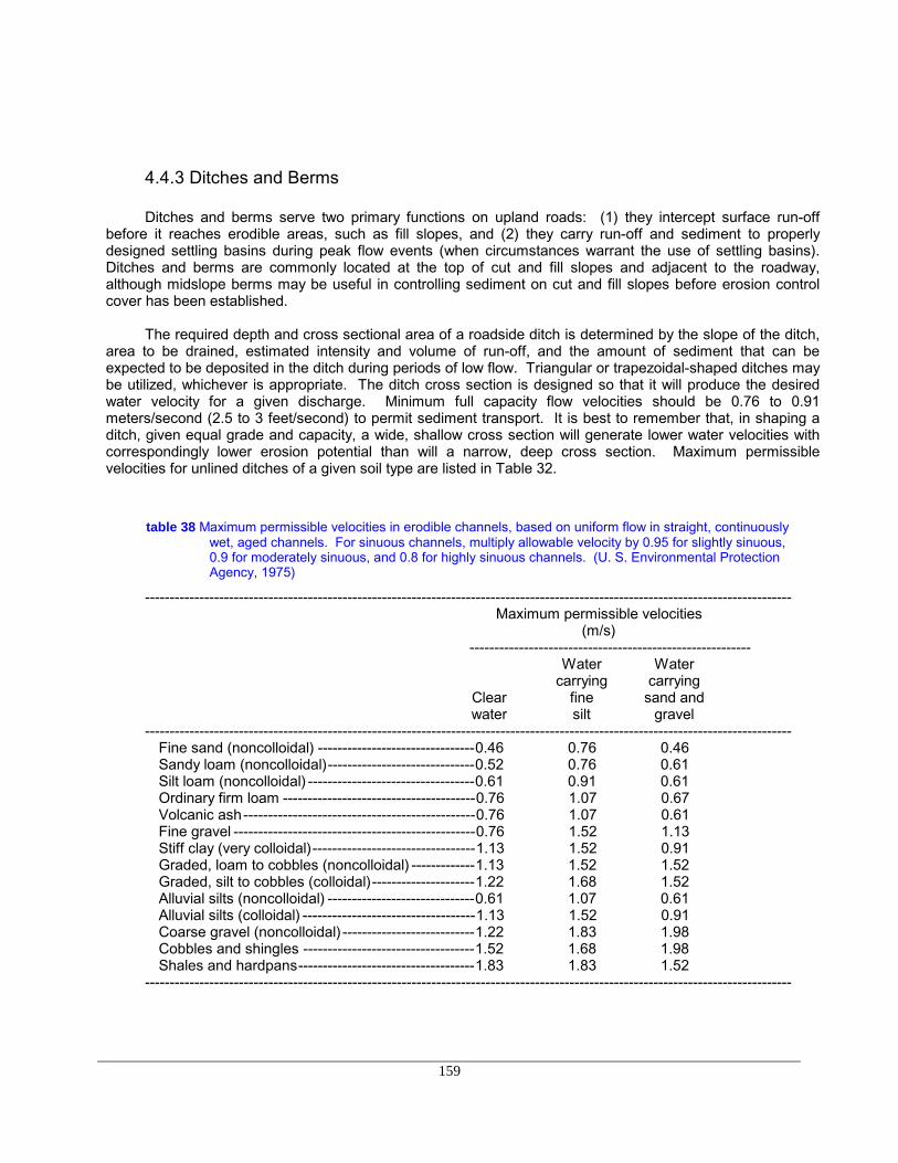
159

4.4.3 Ditches and Berms

Ditches and berms serve two primary functions on upland roads: (1) they intercept surface run-offbefore it reaches erodible areas, such as fill slopes, and (2) they carry run-off and sediment to properlydesigned settling basins during peak flow events (when circumstances warrant the use of settling basins).Ditches and berms are commonly located at the top of cut and fill slopes and adjacent to the roadway,although midslope berms may be useful in controlling sediment on cut and fill slopes before erosion controlcover has been established.

The required depth and cross sectional area of a roadside ditch is determined by the slope of the ditch,area to be drained, estimated intensity and volume of run-off, and the amount of sediment that can beexpected to be deposited in the ditch during periods of low flow. Triangular or trapezoidal-shaped ditches maybe utilized, whichever is appropriate. The ditch cross section is designed so that it will produce the desiredwater velocity for a given discharge. Minimum full capacity flow velocities should be 0.76 to 0.91meters/second (2.5 to 3 feet/second) to permit sediment transport. It is best to remember that, in shaping aditch, given equal grade and capacity, a wide, shallow cross section will generate lower water velocities withcorrespondingly lower erosion potential than will a narrow, deep cross section. Maximum permissiblevelocities for unlined ditches of a given soil type are listed in Table 32.

table 38 Maximum permissible velocities in erodible channels, based on uniform flow in straight, continuouslywet, aged channels. For sinuous channels, multiply allowable velocity by 0.95 for slightly sinuous,0.9 for moderately sinuous, and 0.8 for highly sinuous channels. (U. S. Environmental ProtectionAgency, 1975)

-----------------------------------------------------------------------------------------------------------------------------------Maximum permissible velocities

(m/s)---------------------------------------------------------

Water Watercarrying carrying

Clear fine sand andwater silt gravel

-----------------------------------------------------------------------------------------------------------------------------------Fine sand (noncolloidal) --------------------------------0.46 0.76 0.46Sandy loam (noncolloidal)------------------------------0.52 0.76 0.61Silt loam (noncolloidal) ----------------------------------0.61 0.91 0.61Ordinary firm loam ---------------------------------------0.76 1.07 0.67Volcanic ash-----------------------------------------------0.76 1.07 0.61Fine gravel -------------------------------------------------0.76 1.52 1.13Stiff clay (very colloidal)---------------------------------1.13 1.52 0.91Graded, loam to cobbles (noncolloidal) -------------1.13 1.52 1.52Graded, silt to cobbles (colloidal)---------------------1.22 1.68 1.52Alluvial silts (noncolloidal) ------------------------------0.61 1.07 0.61Alluvial silts (colloidal) -----------------------------------1.13 1.52 0.91Coarse gravel (noncolloidal) ---------------------------1.22 1.83 1.98Cobbles and shingles -----------------------------------1.52 1.68 1.98Shales and hardpans------------------------------------1.83 1.83 1.52

-----------------------------------------------------------------------------------------------------------------------------------

table 39 Manning's n for open ditches.

160

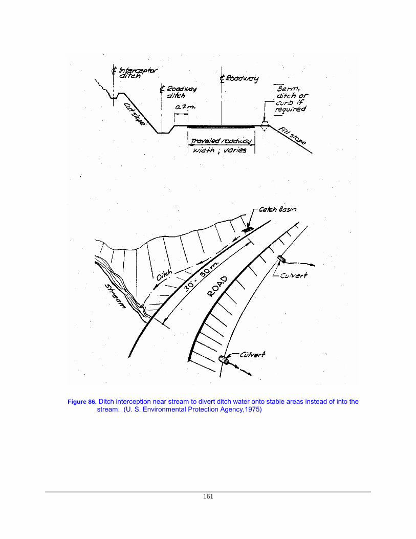
161

Figure 86. Ditch interception near stream to divert ditch water onto stable areas instead of into thestream. (U. S. Environmental Protection Agency,1975)

162

The procedure for calculating flow rates is the same as that discussed in Section 4.2. Thecorresponding roughness factors (Manning's n) for open channels are given in Table 33. Ditches in highlyerodible soils may require riprap, rock rubble lining, jute matting, or grass seeding. Riprap or rubble-linedditches will tend to retard flow enough to allow water movement while retaining the sediment load at low flowperiods. Lining ditches can reduce erosion by as much as 50 percent and may provide economical benefits byreducing the required number of lateral cross drains when materials can be obtained at low cost.

Ditch water should not be allowed to concentrate, nor should it be allowed to discharge directly into livestreams. A cross drain such as a culvert should carry the ditch water across and onto a protected surface(Figure 81). Spacing of ditch relief culverts is discussed in Section 4.4.4 and 4.5.

The ditch grade will normally follow the roadway grade. However, the minimum grade for an unpavedditch should be 1 percent. Runoff intensity or discharge values needed to calculate ditch size can bedetermined by calculations described below for culvert design. However, allowances should be made forsedimentation, plus at least 0.3 m between the bottom of the roadway subgrade and the full flow watersurface. The suggested minimum size of roadside ditches is shown in Figure 87.

12

160 cm

30 cm

TRAPEZOIDAL

40 - 50 cm

11 2

1

90 cm

30 cm

TRIANGULAR

Figure 87. Minimum ditch dimensions.

163

Velocity of the ditch water is a function of cross section, roughness and grade. For a typical triangularcross section the velocity can be calculated from Manning's equation:

V = n-1 * R2/3*S1/2

where V equals velocity in meters/second and the other values are as defined in Chapter 4.2. For atriangular channel with sideslopes of 1:1 and 2:1, flowing 0.3 meters deep, the hydraulic radius, R, equals 0.12m. Table 34 lists ditch velocities as a function of roughness coefficients and grade, and Figure 88 provides anomograph for the solution of Manning's equation.

In most cases ditch lines should be protected to withstand the erosion. For channels with grade steeperthat 10 percent, a combination of cross section widening, surface protection and increased surface roughnessmay be required.

table 40 Ditch velocities for various n and grades. Triangular ditch with side slope ratio of 1:1 and 2:1, flowing0.30 meters deep; hydraulic radius R=0.12.

--------------------------------------------------------------------------------------------------------------------------------n

Slope -------------------------------------------------------------------0.02 0.03 0.04

(%)--------------------------------------------------------------------------------------------------------------------------------

-------------------------meters/sec---------------------2.............................................1.7 1.2 0.94.............................................2.5 1.6 1.26.............................................3.0 2.0 1.58.............................................3.5 2.3 1.710...........................................3.9 2.6 1.912...........................................4.3 2.9 2.115...........................................4.8 3.2 2.418...........................................5.3 3.5 2.6

--------------------------------------------------------------------------------------------------------------------------------

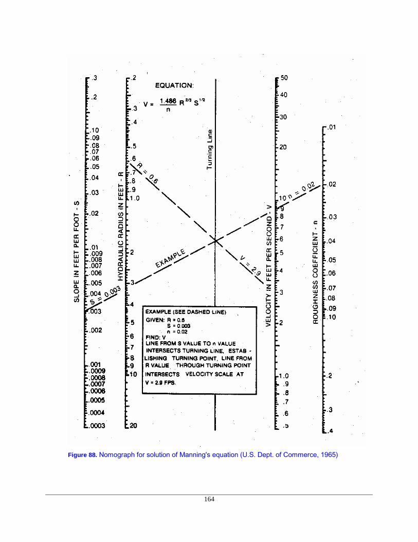
164

Figure 88. Nomograph for solution of Manning's equation (U.S. Dept. of Commerce, 1965)

165

EXAMPLE:

Determine whether the water velocity for a road ditch will be below critical levels for erosion. Ifvelocities are too high, make and evaluate changes (see also U.S. Forest Service, 1980). Ditchdimension is a symmetrical, triangular channel, 0.39 m deep with 2.5:1 slopes with sandy banks (SW)and a slope of 0.003 m/m.

Solution:

1. The hydraulic radius, R, is equal to area divided by wetted perimeter.

R = 0.38 m2/2.1 m = 0.18 m

Converting to english units, divide meters by 0.3 m/ft.

R = 0.60 ft

2. Obtain roughness coefficient from Table 32 (n = 0.020).

3. Obtain maximum allowable velocity 0.46 to 0.76 m/sec (Table 31). Convert to english units bydividing by 0.3 m/ft.

Vmax = 1.5 to 2.5 ft/sec

4. From Figure 88, find the velocity for the specified ditch (2.9 ft/sec). Convert to metric by multiplyingby 0.3m/ft.

Vditch = 0.87 m/sec.

5. Compare the calculated ditch velocity with the maximum recommended velocity for sandy channels:

specified ditch maximum velocity

0.87 m/sec 0.46 - 0.76 m/sec

The ditch has too great a velocity given the conditions stated above. Therefore, measures must betaken that will reduce the water velocity. Water velocity in ditches can be reduced by protecting the channelwith vegetation, rock, or by changing the channel shape. (With vegetative protection, the friction factor (n)becomes 0.030 - 0.050 and the maximum recommended velocity becomes 0.9 - 1.2 m/sec.)

6. Obtain velocity for specified ditch with vegetative protection by referring to Figure 88 (1.9 feet persecond).

7. Compare the calculated ditch velocity with the maximum recommended velocity for vegetationprotected channels (average turf) with easily eroded soils:

specified ditch maximum velocity

0.57 m/sec 0.9 - 1.2 m/sec

8. If the specified ditch has a lower velocity than the recommended maximum velocities, it should bestable as long as the vegetation remains intact.

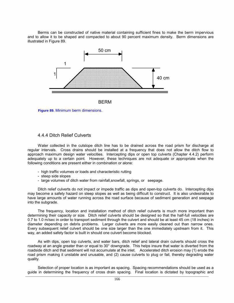
166

Berms can be constructed of native material containing sufficient fines to make the berm imperviousand to allow it to be shaped and compacted to about 90 percent maximum density. Berm dimensions areillustrated in Figure 89.

1

1

50 cm

40 cm

BERM

Figure 89. Minimum berm dimensions.

4.4.4 Ditch Relief Culverts

Water collected in the cutslope ditch line has to be drained across the road prism for discharge atregular intervals. Cross drains should be installed at a frequency that does not allow the ditch flow toapproach maximum design water velocities. Intercepting dips or open top culverts (Chapter 4.4.2) performadequately up to a certain point. However, these techniques are not adequate or appropriate when thefollowing conditions are present either in combination or alone:

- high traffic volumes or loads and characteristic rutting- steep side slopes- large volumes of ditch water from rainfall,snowfall, springs, or seepage.

Ditch relief culverts do not impact or impede traffic as dips and open-top culverts do. Intercepting dipsmay become a safety hazard on steep slopes as well as being difficult to construct. It is also undesirable tohave large amounts of water running across the road surface because of sediment generation and seepageinto the subgrade.

The frequency, location and installation method of ditch relief culverts is much more important thandetermining their capacity or size. Ditch relief culverts should be designed so that the half-full velocities are0.7 to 1.0 m/sec in order to transport sediment through the culvert and should be at least 45 cm (18 inches) indiameter depending on debris problems. Larger culverts are more easily cleaned out than narrow ones.Every subsequent relief culvert should be one size larger than the one immediately upstream from it. Thisway, an added safety factor is built in should one culvert become blocked.

As with dips, open top culverts, and water bars, ditch relief and lateral drain culverts should cross theroadway at an angle greater than or equal to 30° downgrade. This helps insure that water is diverted from theroadside ditch and that sediment will not accumulate at the inlet. Accelerated ditch erosion may (1) erode theroad prism making it unstable and unusable, and (2) cause culverts to plug or fail, thereby degrading waterquality.

Selection of proper location is as important as spacing. Spacing recommendations should be used as aguide in determining the frequency of cross drain spacing. Final location is dictated by topographic and

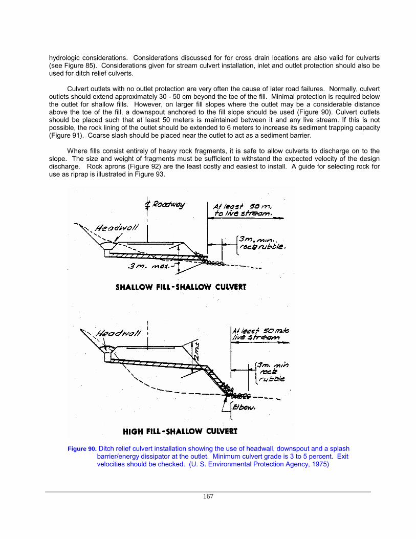
167

hydrologic considerations. Considerations discussed for for cross drain locations are also valid for culverts(see Figure 85). Considerations given for stream culvert installation, inlet and outlet protection should also beused for ditch relief culverts.

Culvert outlets with no outlet protection are very often the cause of later road failures. Normally, culvertoutlets should extend approximately 30 - 50 cm beyond the toe of the fill. Minimal protection is required belowthe outlet for shallow fills. However, on larger fill slopes where the outlet may be a considerable distanceabove the toe of the fill, a downspout anchored to the fill slope should be used (Figure 90). Culvert outletsshould be placed such that at least 50 meters is maintained between it and any live stream. If this is notpossible, the rock lining of the outlet should be extended to 6 meters to increase its sediment trapping capacity(Figure 91). Coarse slash should be placed near the outlet to act as a sediment barrier.

Where fills consist entirely of heavy rock fragments, it is safe to allow culverts to discharge on to theslope. The size and weight of fragments must be sufficient to withstand the expected velocity of the designdischarge. Rock aprons (Figure 92) are the least costly and easiest to install. A guide for selecting rock foruse as riprap is illustrated in Figure 93.

Figure 90. Ditch relief culvert installation showing the use of headwall, downspout and a splashbarrier/energy dissipator at the outlet. Minimum culvert grade is 3 to 5 percent. Exitvelocities should be checked. (U. S. Environmental Protection Agency, 1975)

168

Figure 91. Ditch relief culvert in close proximity to live stream showing rock dike to diffuse ditchwater and sediment before it reaches the stream. (U. S. Environmental Protection Agency,1975)

Figure 92. Energy dissipators. (Darrach, et al., 1981)

169

Figure 93. Size of stone that will resist displacement by water for various velocities and ditch side slopes.

1 ft. = 30 cm (U.S. Dept. of Commerce,1965)

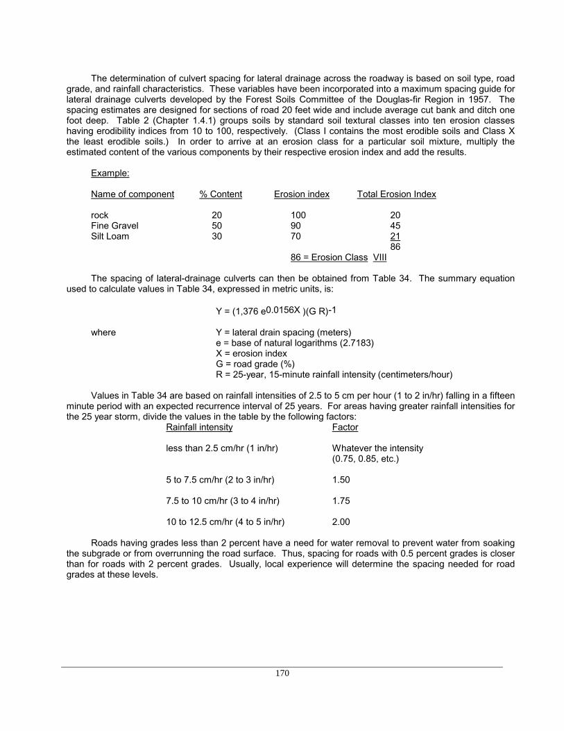
170

The determination of culvert spacing for lateral drainage across the roadway is based on soil type, roadgrade, and rainfall characteristics. These variables have been incorporated into a maximum spacing guide forlateral drainage culverts developed by the Forest Soils Committee of the Douglas-fir Region in 1957. Thespacing estimates are designed for sections of road 20 feet wide and include average cut bank and ditch onefoot deep. Table 2 (Chapter 1.4.1) groups soils by standard soil textural classes into ten erosion classeshaving erodibility indices from 10 to 100, respectively. (Class I contains the most erodible soils and Class Xthe least erodible soils.) In order to arrive at an erosion class for a particular soil mixture, multiply theestimated content of the various components by their respective erosion index and add the results.

Example:

Name of component % Content Erosion index Total Erosion Index

rock 20 100 20Fine Gravel 50 90 45Silt Loam 30 70 21

8686 = Erosion Class VIII

The spacing of lateral-drainage culverts can then be obtained from Table 34. The summary equationused to calculate values in Table 34, expressed in metric units, is:

Y = (1,376 e0.0156X )(G R)-1

where Y = lateral drain spacing (meters)e = base of natural logarithms (2.7183)X = erosion indexG = road grade (%)R = 25-year, 15-minute rainfall intensity (centimeters/hour)

Values in Table 34 are based on rainfall intensities of 2.5 to 5 cm per hour (1 to 2 in/hr) falling in a fifteenminute period with an expected recurrence interval of 25 years. For areas having greater rainfall intensities forthe 25 year storm, divide the values in the table by the following factors:

Rainfall intensity Factor

less than 2.5 cm/hr (1 in/hr) Whatever the intensity(0.75, 0.85, etc.)

5 to 7.5 cm/hr (2 to 3 in/hr) 1.50

7.5 to 10 cm/hr (3 to 4 in/hr) 1.75

10 to 12.5 cm/hr (4 to 5 in/hr) 2.00

Roads having grades less than 2 percent have a need for water removal to prevent water from soakingthe subgrade or from overrunning the road surface. Thus, spacing for roads with 0.5 percent grades is closerthan for roads with 2 percent grades. Usually, local experience will determine the spacing needed for roadgrades at these levels.

tabl

171

e 41 Guide for maximum spacing (in feet) of lateral drainage culverts by soil erosion classes and roadgrade (2% to 18%). (Forest Soils Comm., Douglas Fir Reg., PNW, 1957)

172

4.5. Subsurface drainage

When groundwater cannot be effectively removed or intercepted by surface drainage, subsurfacedrainage techniques are required. As discussed in previous sections of this workbook, if water is not removedfrom subgrade or pavement structures it may create instability, reduce load bearing capacity, increase thedanger of frost action and create a safety hazard by freezing of the traveled surface.

Field investigations carried out during the route reconnaissance and design stages may not alwaysreveal subdrainage problems. These less obvious problems can be effectively dealt with during construction.Field investigations should be carried out during the wet season and may include soil and/or geologic studies,borings or trenches to locate groundwater, inspections of natural and cut slopes in the local area, andmeasurement of discharge when possible. Sites with potential slope stability problems should be morethoroughly evaluated. When groundwater tables approach the ground surface, such as in low, swampy areas,the gradeline should be placed high enough to keep water from being drawn up into the fill by capillary action.Whenever possible, well graded granular materials, such as coarse sand, should be used for fill construction.For a detailed discussion of grading requirements for filter materials the reader is referred to the Earth Manualpublished by the U.S. Department of the Interior (1974).

Three types of subdrainage systems are commonly used:

(1) Pipe underdrains. This system consists of perforated pipe placed at the bottom of a narrow trench andbackfilled with a filter material such as coarse sand. It is generally used along the toes of cut or fillslopes. The trench should be below the groundwater surface and dug into a lower, more inpervious soillayer to intercept groundwater. The drains may be made of metal, concrete, clay, asbestos-cement, orbituminous fiber and should be 15 centimeters (6 inches) in diameter or larger.

(2) Drilled drains. This system consists of perforated metal pipes placed in holes drilled into cut or fillslopes after construction.

(3) French drains. This system consists of trenches backfilled with porous material, such as very coarsesand or gravel. This type of drain is apt to become clogged with fines and is not recommended.

A major difficulty in selecting a drainage system is the lack of adequate performance data for variousdrainage methods. A good knowledge of seasonal groundwater fluctuations, variation in lateral and verticalpermeability, and the ratio of vertical to lateral permeability are critical. Long term monitoring of drainageperformance is important in determining appropriate prescriptions for future installations. For example,perforated drains are commonly prescribed but often will not function properly as a result of clogging of poreswith fines or from geochemical reactions leading to the formation of precipitates. Several methods may beused to prevent plugging depending on soil characteristics and material availability. The first is to enclose theperforated pipe with geotextile fabric. Second, surround the pipe with an open graded aggregate material,which in turn is surrounded by a fabric. The use of fabric eliminates the need for an inverted filter consisting ofvarious sized gravel and sand layers. Third, if fabric is not available, surround the pipe with a gradedaggregate filter. Although the cost of installing such a drainage system is high, it may effectively reduce finalroad costs by decreasing the depth of base rock needed, thereby reducing subgrade widths and associatedcosts for clearing, excavating, and maintenance.

173

LITERATURE CITED

Amimoto, P. Y. 1978. Erosion and sediment control handbook. California Division of Mines and Geology,Department of Conservation. 197 p.

Beschta, R. L. 1981. Streamflow estimates in culverts. Oregon State University, Forest ResearchLaboratory, Res. Note. 67. 4 p.

Darrach, A. G., W. J. Sauerwein, and C. E. Halley. 1981. Building water pollution control into small privateforest and ranchland roads. U. S. Department of Agriculture, Forest Service and Soil ConservationService.

Forest Soils Committee of the Douglas Fir Region. 1957. An introduction to the forest soils of the Douglas-firRegion of the Pacific Northwest. University of Washington.

Highway Task Force. 1971. Handbook of steel drainage and highway construction products (2nd Ed).American Iron and Steel Institute, 150 E 2nd Street, New York. 368 p.

Megahan, W.F. 1977. Reducing erosional impacts of roads. In: Guidelines for Watershed Management.Food and Agriculture Organization, United Nations, Rome. p 237-261.

Minematsu, H. and Y. Minamikata, 1983. Optimum spacing for open - top culverts on forest roads. Universityof Agriculture and Technique, Tokyo. Jour. of J.F.S. 65(12):465-470.

Packer, P. 1967. Criteria for designing and locating logging roads to control sediments. Vol.1, No.13.

Pearce, J. K. 1960. Forest engineering handbook. U. S. Department of Interior, Bureau of LandManagement. 220 p.

Reid, L.M. 1981. Sediment production from gravel-surfaced forest roads, Clearwater basin,Washington. Publ. FRI-UW-8108, Univ. of Washington, Seattle. 247 p.

Searcy, J. K. 1967. Use of riprap for bank protection. Federal Highway Administration, Washington D. C. 43p.

USDA, Forest Service. 1971. Transportation engineering handbook. Handbook No. 7709.11.

_________________. 1979. Technical guide, erosion prevention and control on timber sales areas.Intermountain Region.

Yee, C. S. and T. D. Roelofs. 1980. Planning forest roads to protect salmonid habitat. U. S. Department ofAgriculture, Forest Service. General Technical Report PNW-109. 26 p.

U.S. Dept. of Commerce, Bureau of Public Roads. 1963. Hydraulic Charts for the Selection of HighwayCulverts, Hydraulic Engineering Circular No. 5.

U.S. Dept. of the Interior, Bureau of Reclamation. 1974. Earth Manual, a water resources technicalpublication. Second edition. Government Printing Office, Washington D.C.

174

CHAPTER 5

SURFACE AND SLOPE PROTECTIVE MEASURES

5.1 Introduction

Properly designed slope protection and stabilization has to include two components: a vegetational-biological and a mechanical-structural component. For maximum effect, both components must be integrallyplanned prior to road construction.

Properly designed and planted vegetative covers play a significant role in preventing surface erosionand shallow mass failures. The function of root systems of live plants on shallow soils on steep slopes is thatof a binder for individual soil particles or aggregates. They act in several ways to increase slope stability: (1)they bond unstable soil mantles to stable subsoils or substrata, (2) they provide a cover of a laterally strongfine root systems close to the surface, and (3) they provide localized centers of reinforcement in the vicinity ofindividual trees where embedded stems act like a buttress pile or arch-abutment on a slope.

The structural-mechanical component can consist of conventional retaining walls, either the gravity orcantilever type, or a reinforced earth structure. Structural-mechanical stabilization techniques are called for incases where the potential for deep-seated slope movement or high, lateral earth stresses exists.

A simplified flow chart is shown in Figure 94 which indicates the appropriate combination of methods toeither maintain or achieve a stable and erosion-free slope. Implicit in any slope stability discussion is theeffect of water and the importance of proper drainage. Mechanical drainage structures, such as culverts,ditches, water bars, is discussed in Chapter 4.3, 4.4, and 4.5. In addition to mechanical controls, however,vegetation can provide a form of "biological" drainage through plant transpiration. Root systems caneffectively dewater soil mantles during their active growing season, but often the periods of most danger fromslope failure and erosion do not coincide with peak transpiration periods.

More detailed information concerning biotechnical slope stabilization, the combination of vegetative andstructural components can be found in Gray and Leiser (1982), Volgman (1979) and Schiechtl (1978, 1980).

5.2 Surface Protection Measures

The simplest and most cost effective means of stabilizing bare soil surfaces is through the use ofvegetation or mulches. The objective of all surface stabilization techniques is to establish, as rapidly aspossible, a dense vegetative cover to minimize available sources for sediment. Native plants generallyrequire less expense and maintenance as well as being visually harmonious with the natural landscape. Manyexotic species have been cultivated specifically for erosion protection and may also be suitable.

The body of research that points to road construction as the major cause of stream sedimentation inmountainous environments also indicates that surface erosion on severely disturbed soils such as road fills ishighest immediately following disturbance and decreases rapidly over time. This suggests that stabilizationmeasures must be employed during and immediately following construction. The methods chosen mustprovide rapid benefits hence merely seeding disturbed areas may not provide much relief. Transplanting livingplants, fertilizing or mulching exposed soil surfaces may be required to achieve the desired level of protection.

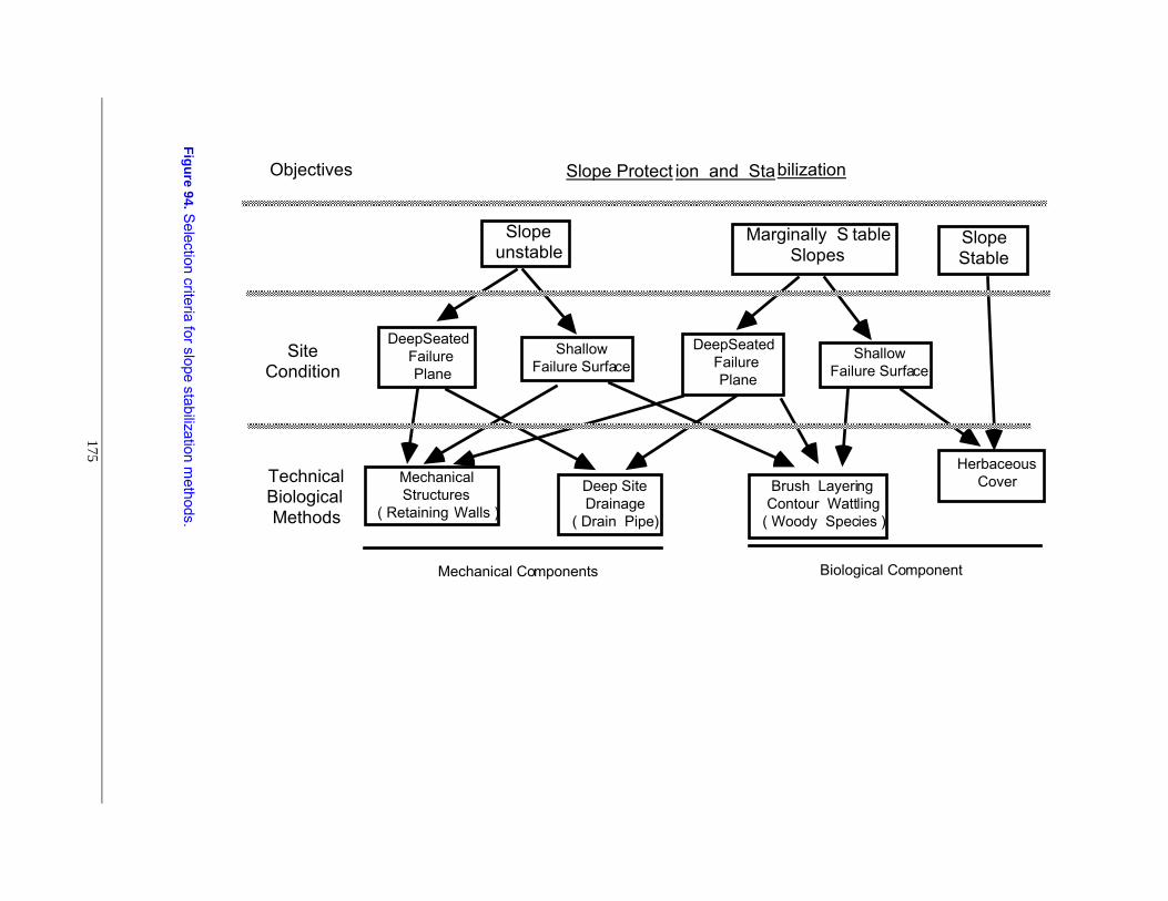
175

Slope Protect ion and StabilizationObjectives

Site Condition

DeepSeated Failure Plane

DeepSeated Failure Plane

Shallow Failure Surface

Shallow Failure Surface

Mechanical Structures

( Retaining Walls )

Deep Site Drainage

( Drain Pipe )

Brush Layering Contour Wattling

( Woody Species )

Herbaceous Cover

Slope unstable

Marginally S table Slopes

Slope Stable

Technical Biological Methods

Mechanical Components Biological Component

Figure 94. Selection criteria for slope stabilization methods.

176

5.2.1 Site Analysis

In order to ensure success of any revegetation effort, it is necessary to prepare an overall plan whichconsiders the climate, vegetation, and microsite (soils, microclimate, slope, and aspect).

Climatic information should center on rainfall frequency distribution and amount. Likewise, averagetemperature, minimum/maximum temperatures, heating degree-days and number of frost free days areimportant points to consider. The vegetation analysis includes the suitability of native or exotic (introduced)plant species for the specific area in question. Here, the focus should be set on inventorying the entirespectrum of plant species that occupy a given site. The survey should note the particular microsites, soils andaspects in which different species grow. Typical points toconsider include:

- which plants do well in a wide range of conditions- which plants make good seed crops- which plants root readily when partially buried or resprout from roots cut during construction- which plants have the best attributes for erosion control(rapid, dense growth; growing season; rooting characteristics).

Microsite evaluation should consider factors such as microclimate, aspect, topography and soils. Themicroclimate is primarily affected by variations in the radiation balance and the immediate surroundings.Changes in the radiation balance will affect microclimate regime and surface temperatures -- two extremelyimportant factors for plant survival. Examples are changing the surface color or establishing a vapor barrier.Installing a vapor barrier to reduce evaporation losses will result in increases in the surface temperature. Bychanging the surface to a light color, the radiation absorbed by the surface can be reduced to compensate forthe temperature rise. For further information on the interaction of microclimate and vegetation, the reader isreferred to Geiger (1961, 1966).

Aspect and topography may reveal the need for specific site treatment either for plant survival and/orlocal site stabilization and slope preparation to allow for plant establishment. Wet and dry areas should bemapped for determining the need for special dewatering treatments or adoption of a particular seed mix.Likewise slope angles greater than 40 degrees are often difficult to revegetate, except in cases where slopesconsist of decomposing bedrock or have a uniform, rocky subsoil. Assessment of the degree of local surfaceerosion (e.g. shallow versus deep seated) will determine the need for shallow rooted plant cover or a moredeeply rooted plant species.

Soil analysis should consider the local soil profile and determine the predominant soil horizon present onthe finished surface. Road cuts or fills may expose layers, strata, or horizons which may be significantlydifferent from the surface soil which supports a given plant species community. Factors to consider are pH,salinity, nutrient levels, and texture (water holding capacity).

5.2.2 Site Preparation

In order to ensure success of any revegetation effort, it is necessary to prepare a proper seedbed. Thismay include reshaping the slope if gravity will cause "ravelling" of loose soil. A 1:1 slope ratio or better isrecommended to provide a good seeding surface. Slopes of 6 meters (20 feet) or more should be broken upwith small ditches or flat benches on the contour. Roughening the slope along the contours will reduce thechance of rilling and will provide small depressions that retain the seed. Oftentimes, construction work or treeand brush removal generally leave sites sufficiently scarified to permit seed to reach mineral soil.

Site preparation efforts on shallow soils may permanently damage the seeding site. The small volumeof soil interlacing rocks may fall in the ditch line and be lost. Likewise, loose soil sidecast on fill slopes isextremely prone to erosion. Compaction of this sidecast material with one pass of a sheepsfoot roller will

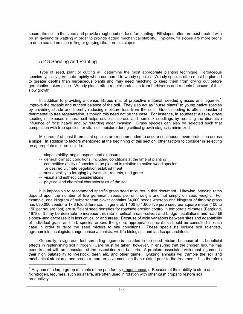
177

secure the soil to the slope and provide roughened surface for planting. Fill slopes often are best treated withbrush layering or wattling in order to provide added mechanical stability. Typically, fill slopes are more proneto deep seated erosion (rilling or gullying) than are cut slopes.

5.2.3 Seeding and Planting

Type of seed, plant or cutting will determine the most appropriate planting technique. Herbaceousspecies typically germinate rapidly when compared to woody species. Woody species often must be plantedto greater depths than herbaceous plants and may need mulching to keep them from drying out beforegermination takes place. Woody plants often require protection from herbivores and rodents because of theirslow growth.

In addition to providing a dense, fibrous mat of protective material, seeded grasses and legumes1improve the organic and nutrient balance of the soil. They also act as "nurse plants" to young native speciesby providing shade and thereby reducing moisture loss from the soil. Grass seeding is often considereddetrimental to tree regeneration, although this need not be the case. For instance, in southeast Alaska, grassseeding of exposed mineral soil helps establish spruce and hemlock seedlings by reducing the disruptiveinfluence of frost heave and by retarding alder invasion. Grass species can also be selected such thatcompetition with tree species for vital soil moisture during critical growth stages is minimized.

Mixtures of at least three plant species are recommended to assure continuous, even protection acrossa slope. In addition to factors mentioned at the beginning of this section, other factors to consider in selectingan appropriate mixture include:

-- slope stability, angle, aspect, and exposure-- general climatic conditions, including conditions at the time of planting-- competitive ability of species to be planted in relation to native weed species or desired ultimate vegetation establishment-- susceptibility to foraging by livestock, rodents, and game-- visual and esthetic considerations-- physical and chemical characteristics of the soil.

It is impossible to recommend specific grass seed mixtures in this document. Likewise, seeding ratesdepend upon the number of live germinant seeds per unit weight and not simply on seed weight. Forexample, one kilogram of subterranean clover contains 34,000 seeds whereas one kilogram of timothy grasshas 590,000 seeds--a 17.3 fold difference. In general, 1,100 to 1,600 live pure seed per square meter (100 to150 per square foot) are sufficient seed densities for roadside erosion control in temperate climates (Berglund,1978). It may be desirable to increase this rate in critical areas--culvert and bridge installations and road fillslopes--and decrease it in less critical or arid areas. Because of wide variations between sites and adaptabilityof individual grass and forb species around the globe, appropriate specialists should be consulted in eachcase in order to tailor the seed mixture to site conditions. These specialists include soil scientists,agronomists, ecologists, range conservationists, wildlife biologists, and landscape architects.

Generally, a vigorous, fast-spreading legume is included in the seed mixture because of its beneficialeffects in replenishing soil nitrogen. Care must be taken, however, in ensuring that the chosen legume hasbeen treated with an innoculant of the associated root bacteria. A problem associated with most legumes istheir high palatability to livestock, deer, elk, and other game. Grazing animals will trample the soil andmechanical structures and create a more erosive condition than existed prior to the treatment. It is therefore 1 Any one of a large group of plants of the pea family (Leguminosae). Because of their ability to store andfix nitrogen, legumes, such as alfalfa, are often used in rotation with other cash crops to restore soilproductivity.

178

recommended that legumes not be included in seed mixtures for sites readily accessible to game animals,cattle, sheep, or goats unless the legume is known to be unpalatable to animals (Adams, et al., 1983).

Road construction oftentimes results in the loss of the very thin mantle of fertile topsoil leaving arelatively infertile residual subsoil. Fertilizers are often required to provide young plants with sufficientnutrients. Again, variability from site to site requires the expertise of a specialist in order to determine properfertilizer selection and application rates. In general, fertilizer prescriptions are developed on the basis of theamount of total nitrogen in the soil. If a soil test shows total nitrogen to be greater than 0.2 percent, nofertilizer is needed.

Fertilization normally occurs together with seeding either prior to or near the end of the rainy season.Two applications--one prior to and one after the rainy season--are extremely effective. Refertilization may alsobe needed in following years due to reductions in vigor of the crop. If fertilizer costs are prohibitive or supplieslimited, it may be desirable to concentrate efforts on such key areas as large fills and culvert and bridgeemplacements.

5.2.4 Application Methods

Techniques used in establishing grasses include hand-operated cyclone seeders, truck-mountedbroadcast seeders, seed drills, and hydroseeders. Drilling is best as it places the seed directly in the soil at acontrolled depth and seeding rate, but may be impossible on steep cut banks and fills. Hydroseeding is theapplication of seed, fertilizer, and mulch in a slurry of some sort of viscous water soluble binder, such as woodfiber, from a truck-mounted tank. This method is most suitable for large areas and steep slopes whereplastering of materials is necessary to achieve uniform coverage. It is also expensive and sometimesimpractical due to climatic, terrain, or road access conditions. Hand planting is generally effective for smallareas and is often the least expensive. Covering the seed with at least 0.5 to 1 centimeter of soil is critical.Rainfall may help cover it, but raking or dragging seeded areas with tire chains, sections of cyclone fence, orsimilar objects is the most effective.

Soils which are heavily disturbed or which have little surface organic material to retard water runoff needprotection afforded by any readily available mulching materials. Such materials include excelsior, straw,shredded logging residue or slash, and slurried wood or ground paper fibers. Excelsior provides the bestprotection but is very expensive. Straw mulch is very effective when applied at a rate of 5.5 metric tons perhectare (2 tons per acre) and secured to the surface either mechanically by punching it into the surface withthe end of a shovel or chemically with a liquid "tackifier" such as emulsified asphalt. Table 36 shows theeffectiveness of different mulches subjected to a rainfall rate of 64 mm (2.5 in) per hour on a 20 percent slopewith 15 cm (6 in) of silt loam over compacted calcareous till. Figure 91 outlines a decision matrix to use inorder to choose the most effective erosion control combination for a given set of site and climatic conditions.

table 43 Erosion control and vegetation establishment effectiveness of various mulches on highways ineastern and western Washington. Soils: silty, sandy and gravelly loams, glacial till consisting ofsand, gravel and compacted silts and clays (all are subsoil materials without topsoil addition).Slope lengths: approximate maximum of 50 m (165 ft). Application rates: Cereal straw - 5,500kg/ha (2 t/ac); Straw plus asphalt - 5,500 kg/ha (2 t/ac) and 0.757 l/kg (200 gal/t), respectively;Wood cellulose fiber - 1,345 kg/ha (1,200 lbs/ac); Sod - bentgrass strips 46 cm (18 in) by 1.8 m (6ft) pegged down every third row.

179

--------------------------------------------------------------------------------------------------------------------------------------Surface Cover

-------------------------------------------------------------------------------------------------------------Straw & Wood

Jute Excelsior Straw Asphalt Asphalt Fiber Sod--------------------------------------------------------------------------------------------------------------------------------------

------------------------------------------- Rating -------------------------------------------Erosion ControlSheet erosion 1:1 slope 9.0 10.0 8.0 10.0 6.0 3.0 10.0Sheet erosion 2:1 slope 9.0 10.0 9.0 10.0 7.0 6.0 10.0Sheet erosion 3:1 + slope 10.0 10.0 10.0 10.0 9.0 10.0 10.0

Rill erosion 1:1 slope 6.0 10.0 8.0 10.0 6.0 3.0 10.0Rill erosion 2:1 slope 8.0 10.0 9.0 10.0 7.0 5.0 -Rill erosion 3:1 + slope 10.0 10.0 10.0 10.0 9.0 10.0 10.0

Slump erosion 1:1 slope 10.0 8.0 6.0 7.0 3.0 3.0 8.0Slump erosion 2:1 slope 10.0 9.0 7.0 8.0 5.0 4.0 9.0Slump erosion 3:1 slope Slumps usually do not occur.

Vegetation Establishment

1.5:1 glacial till cut slope 7.5 9.0 7.5 8.5 7.5 6.0 -

2:1 glacial till cut slope 8.9 9.5 8.0 9.3 8.7 6.2 -

2:1 sandy loam fill slope 9.0 10.0 9.0 10.0 7.5 8.5 10.0

2.5:1 silt loam cut slope 5.0 10.0 - 7.8 6.0 - ---------------------------------------------------------------------------------------------------------------------------------------Effectiveness rating: 10.0 = most effective, 1.0 = not effective.

180

Erosion Risk

low medium

Takifier

Climate

favorable

Site Soil, Moisture

submarginal

Fertilizer + Seed Seed

Mulch + Takifier

Mulch

no no

yes

yes

no

no

yes

yes

Figure 95. Selection criteria for surface cover establishment methods in relation to erosion risk.

When using straw as a mulch, it is recommended that only "clean" straw be used to prevent theintroduction of noxious plants. Wood fiber should be applied at a rate of 1.4 to 1.6 metric tons per hectare (0.5to 0.6 tons per acre). At higher rates, wood fiber improves erosion control but inhibits plant establishment.When mulching follows seed and fertilizer application, rather than in combination with seeding and fertilizing(as is the case sometimes with hydroseeding), there is a much greater chance that seed will be in directcontact with mineral soil and will germinate more readily. Hydroseeding a fiber-seed-water slurry can entrap60-70 percent of the seed in the mulch layer.

181

5.2.5 Wattling and filter strips

Oftentimes grass cover alone is insufficient to prevent erosion on long, steep slopes. Wattling or filterstrips work to break the slope into short segments so that the kinetic energy of water flowing over the surfaceis dissipated. Many different methods and materials can be employed to achieve this objective. Heede(1975) successfully used submerged burlap strips 30 cm (1 ft) wide, placed vertically into the ground on thecontour 0.5 to 1 meter (1.5 to 3 ft) apart from each other to control rilling in semi-desert regions. Filterwindrows can be fabricated from slash accumulated during road construction and can easily be constructedsimultaneously along with the road (Cook and King, 1983). A rough estimate of production rates for windrowconstruction during one demonstration is 52 m/hour (170 ft/hour) using a track-mounted Caterpillar 235hydraulic pull shovel (a large backhoe). Sediment trapping efficiency was estimated at between 75 and 85percent. Windrows in this demonstration consisted of logs not less than 0.45 m (18 in) diameter securedagainst undisturbed stumps, rocks, or trees on fill slopes immediately above and parallel to the toe of theslope. Slash (tops, limbs, and brush not exceeding 15 cm (6 in) in diameter and 3.7 m (12 ft) in length werethen placed above the logs in neat piles (also see Chapter 6.3.3, Figure 119).

Table 36 is included to provide guidance in determining appropriate windrow widths based on the lengthof the slope and type of material used to construct the windrow.

Wattling (Figure 96) consists of combined mechanical and natural stabilization techniques in whichstakes are placed on the contour 0.5 m (1.6 ft) apart and at 1.2 m (4 ft) intervals between rows. A trench isthen dug 20 cm (8 in) wide and 25 cm (10 in) deep against or immediately above the contour stakes. Bundlesof live vegetative materials (such as Salix spp., Bambusa spp., Cassia sepium or other locally availablematerial) 13 cm (5 in) in diameter and 3 m (10 ft) long are placed in the trench overlapping end and tail. Thewattling bundles are then covered with soil so that part of the branches and leaves above ground are leftvisible.It is very important that the soil is worked thoroughly into the interstices of the wattles. During theinstallation workers should walk on the wattles as much as possible to insure maximum compaction andworking the soil into the bundles.

Incorrect installation of wattles may actually aid in soil slumping because of collection of water in thewattle trenches. It is therefore important that soil is thoroughly worked into the wattles andno trench remains to be filled with water. Likewise firm staking is important particularly in areas where frostheaving is a problem. An average 10 person crew can treat 200 m2 to 250 m2 (2,000 to 2,500 ft2) in a day(Sheng, 1977b). More detailed information on wattling procedure and installation can also be found in Kraebel(1936), Grey and Leiser (1982), and Schiechtl(1978,1980).

182

table 44 Windrow protective strip widths required below the shoulders1 of 5 year old2 forest roads built onsoils derived from basalt3, having 9 m cross-drain spacing4, zero initial obstruction distance5, and100 percent fill slope cover density6.

(U. S. Environmental Protection Agency, 1975)---------------------------------------------------------------------------------------------------------------------------------------

Obstruction Protective windrow width by type of obstructionspacing ------------------------------------------------------------------------------------------------------------

Depressions Trees and Slash and Herbaceousor mounds Logs Rocks stumps brush vegetation

--------------------------------------------------------------------------------------------------------------------------------------- ---------------------------------------------------- meters ----------------------------------------------------

0.3 10.6 11.2 11.6 12.1 12.5 13.10.6 11.3 12.2 13.1 14.0 14.9 15.90.9 11.9 13.1 14.3 15.9 17.4 18.61.2 12.2 14.0 15.9 17.7 19.5 21.31.5 12.5 14.6 17.0 19.2 21.6 23.81.8 15.2 18.0 20.7 23.5 26.22.1 15.9 18.9 22.2 25.6 28.72.4 16.2 19.8 23.5 27.1 30.82.7 16.5 20.4 24.7 29.0 32.93.0 25.9 30.5 35.13.4 27.8 31.7 36.93.7 38.7

---------------------------------------------------------------------------------------------------------------------------------------1 For protective strip widths from centerlines of proposed roads, increase widths by one-half the

proposed road width.2 If storage capacity of obstructions is to be renewed when roads are 3 years old, reduce protective

strip width by 7 m.3 If soil is derived from andesite, increase protective strip width by 30 cm; from glacial till, increase 1 m;

from hard sediments, increase 2.4 m; from granite, increase 2.5 m; from loess, increase 7 m.4 For each increase in cross-drain spacing beyond 9 m, increase protective strip width 30 cm.5 For each 1.5 m increase in distance to the initial obstruction beyond zero (or the road shoulder),

increase protective strip width 1.2 m.6 For each 10 percent decrease in fill slope cover below a density of 100 percent, increase protective

strip width 0.30 m.

183

Figure 96. Preparation and installation procedure for contour wattling, using live willow stakes (afterKraebel, 1936).

5.2.6 Brush Layering

Contour brush layering (Figure 97) involves embedding green branches of shrubs or trees onsuccessive horizontal layers into the slope. Brush layering is different from wattling in that (1) branches areplaced into the slope perpendicular to the strike instead of parallel creating better resistance to shallow shearfailure, (2) staking is not required, (3) brush layers and surfaces can be reinforced with wire mesh or othermaterial, (4) brush layers can be incorporated into the construction process of a fill. That is, brush layers arelaid down, the next lift of soil is placed and compacted, and the process is repeated.

Contour brush layering is comparable to the "reinforced earth" concept where the cuttings or branchesact in the same fashion as the reinforcing strips.

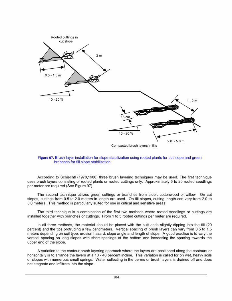
184

10 - 20 %

10 - 20 %

2.0 - 5.0 m

15 cm

Compacted brush layers in fills

2 m

1 - 2 m

Rooted cuttings in cut slope

0.5 - 1.5 m

Figure 97. Brush layer installation for slope stabilization using rooted plants for cut slope and greenbranches for fill slope stabilization.

According to Schiechtl (1978,1980) three brush layering techniques may be used. The first techniqueuses brush layers consisting of rooted plants or rooted cuttings only. Approximately 5 to 20 rooted seedlingsper meter are required (See Figure 97).

The second technique utilizes green cuttings or branches from alder, cottonwood or willow. On cutslopes, cuttings from 0.5 to 2.0 meters in length are used. On fill slopes, cutting length can vary from 2.0 to5.0 meters. This method is particularly suited for use in critical and sensitive areas

The third technique is a combination of the first two methods where rooted seedlings or cuttings areinstalled together with branches or cuttings. From 1 to 5 rooted cuttings per meter are required.

In all three methods, the material should be placed with the butt ends slightly dipping into the fill (20percent) and the tips protruding a few centimeters. Vertical spacing of brush layers can vary from 0.5 to 1.5meters depending on soil type, erosion hazard, slope angle and length of slope. A good practice is to vary thevertical spacing on long slopes with short spacings at the bottom and increasing the spacing towards theupper end of the slope.

A variation to the contour brush layering approach where the layers are positioned along the contours orhorizontally is to arrange the layers at a 10 - 40 percent incline. This variation is called for on wet, heavy soilsor slopes with numerous small springs. Water collecting in the berms or brush layers is drained off and doesnot stagnate and infiltrate into the slope.

185

Installation procedures typically proceed from bottom to top. Fill slope installation is simple. However,care should be taken that the brush layer dips into the slope at least 20 percent. The next soil layer is placedon top and compacted. Cut slope installation requires the opening of a ditch or berm. As with fills, workprogresses from bottom to top. The excavation of the upper berm is used for filling-in and covering the lowerbrush layer.

5.2.7. Mechanical Treatment

Mechanical surface stabilization measures consist of diversion ditches and terraces, serrations, orscarification and can be used in conjunction with vegetative methods discussed above. These methodsgenerally require detailed engineering design and location. T. C. Sheng (1977a) discusses several differentmethods for the construction of bench terraces together with tables providing design information and costs.

Serrations consist of steps of 60 to 120 cm (2 to 4 ft) cut vertically and horizontally along the normal,intended slope gradient. After treatment, the slope is seeded, fertilized, and mulched as discussed in Chapter5.2.3. The steps provide improved seedbeds free of sliding forces normally experienced on steep slopes.Serrations are only effective on cut slopes of soft rock or similar material that will stand vertically or nearvertically for a few years in cut heights of approximately one meter. Likewise, this method is not applicable tosoil types where the rate of slough is so high that vegetative cover is buried and destroyed. If acceptableslope material is soft, the slope should be allowed to slough before seeding until about one-third of the stepsare filled. Otherwise, grass may be destroyed by the excessive rate of initial slough.

Roughened or scarified slopes may not be as esthetically pleasing to the eye as smoothly graded cutand fill slopes, but they are far more effective in increasing infiltration and impeding runoff. Scarified slopesalso provide small depressions for the retention of seed and also help mulch to better adhere to the slope.Roughening may be accomplished by several means including deep cleated bulldozers traveling up and downthe slope, sheepsfoot rollers, rock rippers, and brush rakes mounted on bulldozers. The path of theroughened slope should trend perpendicular to the direction of flow.

5.3 Mass Movement Protection

Deep seated mass failures can be dealt with in three ways. The methods are categorized by the waythey affect soil stability.

1. Avoidance Methods: Relocate road on a more stable area (for large, unstable fills probably by far themost appropriate approach).

2. Reducing Shear Stress: This is achieved through excavation of unacceptable materials. It creates areduction in soil weight and can be accomplished by: a) removal of soil mass at the top of the potentialslide, b) flattening of cut slopes above the road, c) benching of cut slopes.

3. Increasing Shear Strength: This is achieved through retaining structures. They can be grouped into a)rock buttresses at the toe of fill slope, b) cribs or gravity retaining walls at toe of fill or cut, and c) pilingwalls, likewise at the toe of fills or cuts.

Engineering and structural methods for stabilizing slopes can be grouped into four categories:

1. Excavation and filling techniques. This would include excavating the toe of an earth flow untilsuccessive failures result in a stable slope, removing and replacing failed material with lighter, morestable material, or recompacted debris, excavating to unload upper portions of a mass failure, and fillingto load the lower portions of a mass failure (most likely in conjunction with other loading or restrainingstructures).

186

2. Drainage techniques. This would include efforts to remove or disperse surface water (as discussed inChapter 4), drainage of tension cracks, using rock fill underlain by filter cloth to prevent upwardmigration of water into the road prism, insertion of trench drains, perforated, horizontal drains, ordrainage galleries, insertion of vertical drains or wells discharged by syphons, or pumps, and electro-osmosis (the use of direct current passing between wellpoints and steel rods placed midway betweenthe rods to increase the drainage rate) for drainage of low permeability soils.

3. Restraining structures. These include retaining walls, piles, buttresses, counterweight fills, cribs, binwalls, reinforced earth, and pre-stressed or post-tensioned soil or rock anchors (Figure 98).Organizations such as highway departments and railroads have developed charts and tables givingearth pressures for the design of retaining walls that require a minimum of computation. Nearly all ofthese charts and tables are based on the Rankine formula, which describes earth pressures as afunction of unit weight and internal angle of friction of the backfill material.

4. Miscellaneous techniques. Grouting can be used to reduce soil permeability, thereby preventing theingress of groundwater into a failure zone. Chemical stabilization, generally in the form of ion exchangemethods, is accomplished by high pressure injection of specific ion exchange solutions into failurezones or into closely spaced pre-drillled holes throughout the movement zone. Heating or baking ofclay soils can sometimes improve their strength, and, rarely, freezing of soils will help gain temporarystability. Localized electro-osmosis can be used to form in situ anchors or tie-backs. Suppression ofnatural electro-osmosis can be used to reduce unfavorable groundwater pressures. Blasting issometimes used to disrupt failure surfaces and to improve drainage.

For correcting cut or fill failures, a detailed investigation into the reason for the failure, particularly theposition and geometry of the failure surface and other potential failure surfaces, is required prior to prescribingameliorative measures. The neutral line concept, discussed by Hutchinson (1977) and Sidle, et al. (1985), isof particular interest in assessing the impact of cuts and fills on factors of safety. The neutral line describeswhere the load attributed to fill material will have no effect on the original factor of safety. If the load falls up-slope of the neutral line, the factor of safety will decrease; if it is downslope of the neutral line, the factor ofsafety will decrease.

The use of any of these stabilization techniques requires extensive site specific investigations into themechanics of soils, groundwater, and bedrock occurring on the site. It is advisable to utilize the mostexperienced geotechnical or highway engineer available in order to provide the most effective design possible.As can be inferred from the above discussion, any of these techniques will be quite costly to design and install.Furthermore, the success of such measures in functioning adequately through time is highly dependent on theskill of the design engineer and the degree of maintenance employed after construction. Hence, avoidance ofareas where structural stabilization measures are required will result in considerable short term and long termcost savings, and the major opportunity for reducing landslide risk is at the route planning stage.

The purpose of a retaining structure is to provide stability against sliding or failure and protection againstscour and erosion of a slope, or the toe or cutface. The typical retaining structure on forest roads is a gravityretaining wall, which resists earth pressure by the force of its own weight. Excavation and/or fill volume can besignificantly reduced particularly on steep side slopes (see also discussion in Chapter 3.2).

The volume of cribs or retaining walls should be 1/6 to 1/10 of that of the total moving mass to beretained. As a rule, the foundation or base should at least extend 1.2 to 2.0 meters below the slip plane inorder to be effective.

The forces acting on a retaining wall are similar to those acting on a natural slope. These forces are begrouped into resisting forces (forces resisting failure) and driving forces (forces causing failure) as illustratedin Figure 99.

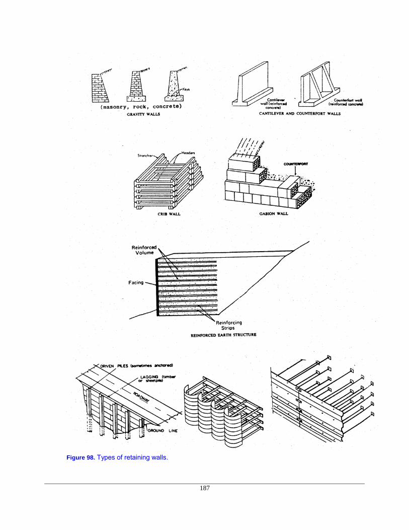
187

Figure 98. Types of retaining walls.

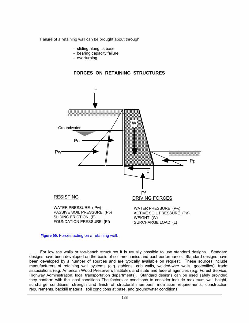
188

Failure of a retaining wall can be brought about through

- sliding along its base- bearing capacity failure- overturning

L

Pa

Pw

WW

Pp

Pf

F

RESISTING

WATER PRESSURE ( Pw) PASSIVE SOIL PRESSURE (Pp) SLIDING FRICTION (F) FOUNDATION PRESSURE (Pf)

DRIVING FORCES

WATER PRESSURE (Pw) ACTIVE SOIL PRESSURE (Pa) WEIGHT (W) SURCHARGE LOAD (L)

FORCES ON RETAINING STRUCTURES

Groundwater

Figure 99. Forces acting on a retaining wall.

For low toe walls or toe-bench structures it is usually possible to use standard designs. Standarddesigns have been developed on the basis of soil mechanics and past performance. Standard designs havebeen developed by a number of sources and are typically available on request. These sources includemanufacturers of retaining wall systems (e.g. gabions, crib walls, welded-wire walls, geotextiles), tradeassociations (e.g. American Wood Preservers Institute), and state and federal agencies (e.g. Forest Service,Highway Administration, local transportation departments). Standard designs can be used safely providedthey conform with the local conditions The factors or conditions to consider include maximum wall height,surcharge conditions, strength and finish of structural members, inclination requirements, constructionrequirements, backfill material, soil conditions at base, and groundwater conditions.

189

An example of a standard log crib wall is shown in Figure 100. A thorough discussion of timber walls isprovided by Schuster et al. (1973). Timber crib walls and gabion structures can withstand some limited,differential base settlement without a significantly affecting the retaining action.Drainage characteristics of thebackfill and crib material is important because of potential water pressure build-up. Most standard designsassume free draining sand or gravel fills.

Gabions are rectangular containers made of heavy steel wire and filled with cobble-sized rocks (10 to 30cm in diameter). A typical gabion retaining wall is shown in Figure 101. Advantages of gabion structures areease of construction, tolerance of uneven settlement, and good drainage characteristics. Gabion walls areparticularly suited in areas where only small, fragmented rocks are available. Typically, they can be builtwithout heavy equipment. Both crib and gabion walls lend themselves to incorporation of vegetative systemsto provide additional strength over time as well as providing a more esthetically pleasing appearance.

Gravity retaining structures utilizing standard designs are typically limited to a height of less than 6.0meters. Structures requiring a larger height have to be designed based on site-specific soil mechanicalconditions.

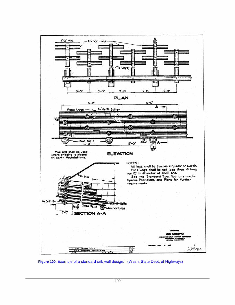
190

Figure 100. Example of a standard crib wall design. (Wash. State Dept. of Highways)

191

Figure 101. Low gabion breast walls showing sequence of excavation, assembly, and filling. (FromWhite and Franks,1978)

LITERATURE CITED

Adams, T. E. and B. L. Kay. 1983. Seeding for erosion control in mountain areas of California. CooperativeExtension, Univ. of California. Leaflet No. 21356. 3 p.

Berglund, E. R. 1978. Seeding to control erosion along forest roads. Oregon State University ExtensionService. Circular No. 885. 19 p.

Bowers, H.D. 1950. Erosion control on California highways, State of California, Dept. of Public Works, Div. ofHighways, Sacramento, Calif. 70 pp.

Cook, M. J., and J. G. King. 1983. Construction cost and erosion control effectiveness of filter windrows on fillslopes. US Dept. of Agriculture Forest Service. Research Note INT-335, Intermountain Forest andRange Experiment Station, Ogden, Utah. 5 p.

Geiger, R. 1961. Das Klima der bodennahen Luftschicht. Friedrich Vieweg and Sohn, Braunschweig,Germany. (English translation, 1968. The climate near the ground. Harvard University Press.)

Gray, D. H. and A.T. Leiser, 1982. Biotechnical slope protection and erosion control. Van Nostrand ReinholdCompany, New York. 271p.

192

Heede, B. H. 1975. Submerged burlap strips aided rehabilitation of disturbed semi-arid sites in Colorado andNew Mexico. US DA, Forest Service. Research Note RM-302. 8 p.

Hutchinson, J. N. 1977. Assessment of the effectiveness of corrective measures in relation to geologicalconditions and types of slope movement. Bull. Int. Assoc. Eng. Geol., 16, pp 131-155.

Kraebel, C.J. 1936. Erosion control on mountain roads. USDA Circular No. 380, Wahington D. C., 43p.

Kuonen, v. 1983. Wald und Gueterstrassen. Eigenverlag CH - 81222 Pfaffhausen, Switzerland 743p.

Schiechtl, H. M. 1980. Bioengineering for land reclamation and conservation. The University of AlbertaPress, Edmonton, Canada. 404 p.

Schiechtl, H.M. 1973. Sicherungsarbeiten im Landdschaftsbau. Grundlagen, lebende Baustoffe, Methoden.Callway, Munich. 244 p.

Sheng, T. C. 1977a. Protection of cultivated slopes: terracing steep slopes in humid regions. In: Guidelinesfor Watershed Management. Food and Agriculture Organization of the United Nations, Rome, Italy. p.147-171.

Sheng, T. C. 1977b. Wattling and staking. In: Guidelines for Watershed Management. Food and AgricultureOrganization of the United Nations, Rome, Italy. p. 289-293.

Sidle, R. C., A. J. Pearce, and C. L. O'Loughlin. 1985. Hillslope Stability and Land Use. Wat. Res. Mon. Ser.,No. 11., Am. Geophys. Un., Washington, D. C. 140 p.

US Environmental Protection Agency. 1975. Logging Roads and Protection of Water Quality. EPA 910/9-75-007. 312 p.

Volgmann, W. 1979. Landschaftsbau. Verlag Ulmer, Stuttgart, Fed. Rep. Germany, 280 p.

Washington State Highway Dept., Olympia, Washington.

White, C.A., and A. L. Franks, 1978. Demonstration of erosion and sediment control technology, Lake TahoeRegion of California, State Water Resoources Control Board, Final Report, 393 pp.

USDA, Forest Service. 1973. Transportation Engineering Handbook, Slope Design Guide. Handbook No.7709.11

193

CHAPTER 6

ROAD CONSTRUCTION TECHNIQUES

6.1 Road Construction Techniques

6.1.1 Construction Staking

Prior to the construction activity the design information has to be moved from the plan to the ground.This is accomplished by staking. Slope stakes are an effective way to insure compliance with the designstandards and to keep soil disturbance to an absolute minimum. Various staking methods can be employed.(Dietz et al., 1984; Pearce, 1960) The method discussed here is but one example.

Stakes, marking various road design points, are typically obliterated during the clearing and grubbingphase. In order to relocate the stakes (centerline, slope stakes) it is helpful to establish reference pointsoutside the clearing limits. Reference points should be set at least 3 to 5 meters behind the uphill clearinglimits. On the average, reference points (or RP's) should be set at least every 70 to 100 meters. Typically,reference points are placed at points where the centerline alignment can be easily re-established, such aspoints of curvature. Figure 102 shows the necessary stakes and stake notation needed by the equipmentoperator to construct a road.

Stakes are used by the equipment operator in locating where to begin cutting. If the selected startingpoint is too high, considerably more material has to be cut in order to construct the proper subgrade (Figure103). For example, if the cut results in a 20 percent wider subgrade, approximately 50 percent more volumehas to be excavated. (See Section 3.2.2.) If the cut is placed too low, an oversteepened cut slope or extraside casting may result, both of which are undesirable.

Starting the cut at the proper point becomes more important as the side slope increases. As a rule,slope stakes should be set when sideslopes exceed 40 to 45 percent depending on the sensitivity of the areaand the operator's experience.

The use of RP's (Reference Points)or slope stakes for proper excavation is shown in Figure 104. Here,the engineer stands on the preliminary centerline of the construction grade and sights for the RP. A slopereading of 30 percent and a slope distance of 5.53 m is recorded. Converting the slope distance of 5.53 m toa horizontal distance of 5.30 m and to a vertical distance of 1.59 m allows the engineer to determine howmuch the "present" or preliminary centerline has to be shifted to conform with the design centerline. The RPtag requires 6.50 m horizontal distance to centerline with a vertical drop of 4.80 m. From that information, itcan be seen that an additional 1.56 m [4.80 - (1.59 + 1.65) = 1.56] has to be cut and the present location hasto be shifted by 1.2 m (6.50 - 5.30 = 1.20). Height of instrument or eye-level is assumed to be 1.65 m.

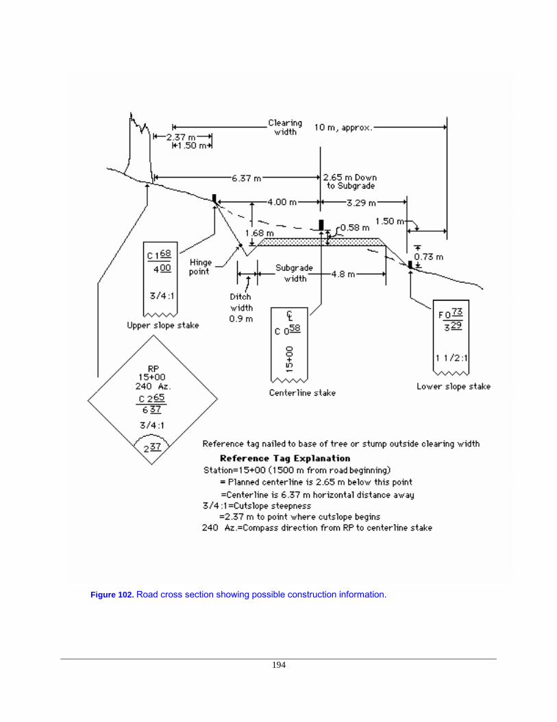
194

Figure 102. Road cross section showing possible construction information.

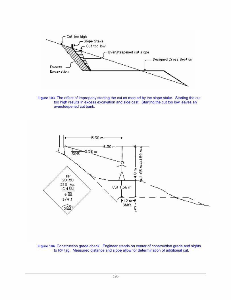
195

Figure 103. The effect of improperly starting the cut as marked by the slope stake. Starting the cuttoo high results in excess excavation and side cast. Starting the cut too low leaves anoversteepened cut bank.

Figure 104. Construction grade check. Engineer stands on center of construction grade and sightsto RP tag. Measured distance and slope allow for determination of additional cut.

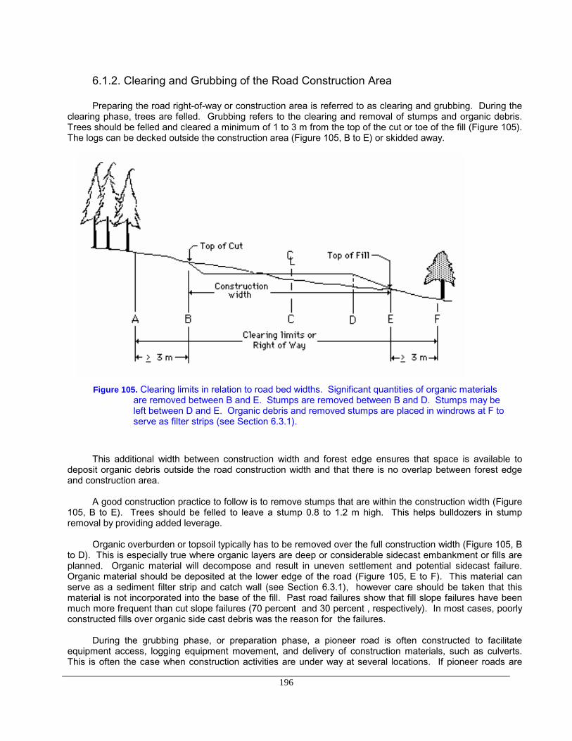
196

6.1.2. Clearing and Grubbing of the Road Construction Area

Preparing the road right-of-way or construction area is referred to as clearing and grubbing. During theclearing phase, trees are felled. Grubbing refers to the clearing and removal of stumps and organic debris.Trees should be felled and cleared a minimum of 1 to 3 m from the top of the cut or toe of the fill (Figure 105).The logs can be decked outside the construction area (Figure 105, B to E) or skidded away.

Figure 105. Clearing limits in relation to road bed widths. Significant quantities of organic materialsare removed between B and E. Stumps are removed between B and D. Stumps may beleft between D and E. Organic debris and removed stumps are placed in windrows at F toserve as filter strips (see Section 6.3.1).

This additional width between construction width and forest edge ensures that space is available todeposit organic debris outside the road construction width and that there is no overlap between forest edgeand construction area.

A good construction practice to follow is to remove stumps that are within the construction width (Figure105, B to E). Trees should be felled to leave a stump 0.8 to 1.2 m high. This helps bulldozers in stumpremoval by providing added leverage.

Organic overburden or topsoil typically has to be removed over the full construction width (Figure 105, Bto D). This is especially true where organic layers are deep or considerable sidecast embankment or fills areplanned. Organic material will decompose and result in uneven settlement and potential sidecast failure.Organic material should be deposited at the lower edge of the road (Figure 105, E to F). This material canserve as a sediment filter strip and catch wall (see Section 6.3.1), however care should be taken that thismaterial is not incorporated into the base of the fill. Past road failures show that fill slope failures have beenmuch more frequent than cut slope failures (70 percent and 30 percent , respectively). In most cases, poorlyconstructed fills over organic side cast debris was the reason for the failures.

During the grubbing phase, or preparation phase, a pioneer road is often constructed to facilitateequipment access, logging equipment movement, and delivery of construction materials, such as culverts.This is often the case when construction activities are under way at several locations. If pioneer roads are

197

constructed, they are often built at the top of the construction width and are usually nothing more than abulldozer trail. When considerable side hill fill construction is planned, however, the dozer trail should belocated at the toe or base of the proposed fill. The trail will serve as a bench and provide a catch for the fill tohold on (Figure 106).

Figure 106. Pioneer road location at bottom of proposed fill provides a bench for holding fill materialof completed road.

6.2 General Equipment Considerations

The method and equipment used in road construction is an important economic and design factor inroad location and subsequent design. A road to be built by an operator whose only equipment is a bulldozerrequires a different design than a road to be built by a contractor equipped with hydraulic excavator, scrapers,and bulldozer. Table 38 lists common road construction equipment and their suitability for the different phasesof road construction. A bulldozer can be used in all phases of road construction from excavation and drainageinstallation to final grading. The front-end loader performs well in soft material. Front-end log loaders can befitted with a bucket extending their usefulness under the correct conditions.

6.2.1 Bulldozer in Road Construction

Probably the most common piece of equipment in forest road construction is the bulldozer equipped withstraight or U-type blades. These are probably the most economical pieces of equipment when material has tobe moved a short distance. The economic haul or push distance for a bulldozer with a straight blade is from17 to 90 meters depending on grade. The road design should attempt to keep the mass balance points withinthese constraints.

The road design should consider the following points when bulldozers are to be used for roadconstruction.

1. Roads should be full benched. Earth is side cast and then wasted rather than used to build up side castfills.

2. Earth is moved down-grade with the aid of gravity, not up-grade.

3. Fill material is borrowed rather than pushed or hauled farther than the economic limit of the bulldozer.

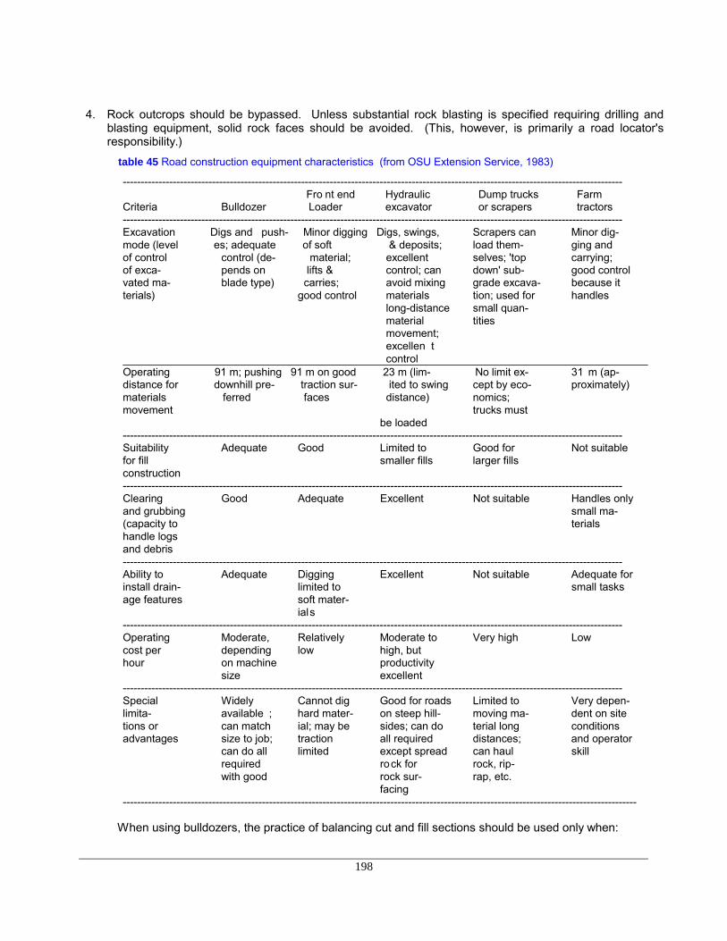
198

4. Rock outcrops should be bypassed. Unless substantial rock blasting is specified requiring drilling andblasting equipment, solid rock faces should be avoided. (This, however, is primarily a road locator'sresponsibility.)

table 45 Road construction equipment characteristics (from OSU Extension Service, 1983)

-------------------------------------------------------------------------------------------------------------------------------------------- Fro nt end Hydraulic Dump trucks Farm

Criteria Bulldozer Loader excavator or scrapers tractors--------------------------------------------------------------------------------------------------------------------------------------------Excavation Digs and push- Minor digging Digs, swings, Scrapers can Minor dig-mode (level es; adequate of soft & deposits; load them- ging andof control control (de- material; excellent selves; 'top carrying;of exca- pends on lifts & control; can down' sub- good controlvated ma- blade type) carries; avoid mixing grade excava- because itterials) good control materials tion; used for handles

long-distance small quan- material tities movement; excellen t control

Operating 91 m; pushing 91 m on good 23 m (lim- No limit ex- 31 m (ap-distance for downhill pre- traction sur- ited to swing cept by eco- proximately)materials ferred faces distance) nomics;movement trucks must

be loaded--------------------------------------------------------------------------------------------------------------------------------------------Suitability Adequate Good Limited to Good for Not suitablefor fill smaller fills larger fillsconstruction--------------------------------------------------------------------------------------------------------------------------------------------Clearing Good Adequate Excellent Not suitable Handles onlyand grubbing small ma-(capacity to terialshandle logsand debris--------------------------------------------------------------------------------------------------------------------------------------------Ability to Adequate Digging Excellent Not suitable Adequate forinstall drain- limited to small tasksage features soft mater-

ials--------------------------------------------------------------------------------------------------------------------------------------------Operating Moderate, Relatively Moderate to Very high Lowcost per depending low high, buthour on machine productivity

size excellent--------------------------------------------------------------------------------------------------------------------------------------------Special Widely Cannot dig Good for roads Limited to Very depen-limita- available ; hard mater- on steep hill- moving ma- dent on sitetions or can match ial; may be sides; can do terial long conditionsadvantages size to job; traction all required distances; and operator

can do all limited except spread can haul skillrequired rock for rock, rip-with good rock sur- rap, etc.

facing------------------------------------------------------------------------------------------------------------------------------------------------

When using bulldozers, the practice of balancing cut and fill sections should be used only when:

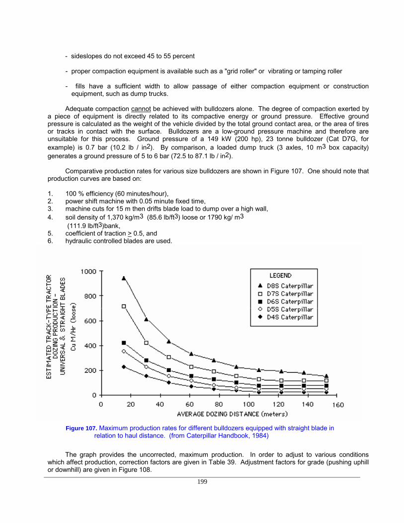
199

- sideslopes do not exceed 45 to 55 percent

- proper compaction equipment is available such as a "grid roller" or vibrating or tamping roller

- fills have a sufficient width to allow passage of either compaction equipment or constructionequipment, such as dump trucks.

Adequate compaction cannot be achieved with bulldozers alone. The degree of compaction exerted bya piece of equipment is directly related to its compactive energy or ground pressure. Effective groundpressure is calculated as the weight of the vehicle divided by the total ground contact area, or the area of tiresor tracks in contact with the surface. Bulldozers are a low-ground pressure machine and therefore areunsuitable for this process. Ground pressure of a 149 kW (200 hp), 23 tonne bulldozer (Cat D7G, forexample) is 0.7 bar (10.2 lb / in2). By comparison, a loaded dump truck (3 axles, 10 m3 box capacity)generates a ground pressure of 5 to 6 bar (72.5 to 87.1 lb / in2).

Comparative production rates for various size bulldozers are shown in Figure 107. One should note thatproduction curves are based on:

1. 100 % efficiency (60 minutes/hour),2. power shift machine with 0.05 minute fixed time,3. machine cuts for 15 m then drifts blade load to dump over a high wall,4. soil density of 1,370 kg/m3 (85.6 lb/ft3) loose or 1790 kg/ m3

(111.9 lb/ft3)bank,5. coefficient of traction > 0.5, and6. hydraulic controlled blades are used.

Figure 107. Maximum production rates for different bulldozers equipped with straight blade inrelation to haul distance. (from Caterpillar Handbook, 1984)

The graph provides the uncorrected, maximum production. In order to adjust to various conditionswhich affect production, correction factors are given in Table 39. Adjustment factors for grade (pushing uphillor downhill) are given in Figure 108.

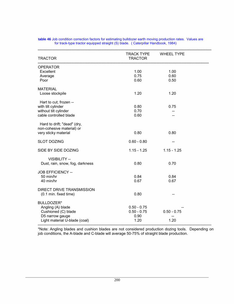
200

table 46 Job condition correction factors for estimating bulldozer earth moving production rates. Values arefor track-type tractor equipped straight (S) blade. ( Caterpillar Handbook, 1984)

---------------------------------------------------------------------------------------------------------------------------------------TRACK TYPE WHEEL TYPE

TRACTOR TRACTOR-------------------------------------------------------------------------------------------------------------------------------------OPERATOR Excellent 1.00 1.00 Average 0.75 0.60 Poor 0.60 0.50

MATERIAL Loose stockpile 1.20 1.20

Hart to cut; frozen --with tilt cylinder 0.80 0.75without tilt cylinder 0.70 --cable controlled blade 0.60 --

Hard to drift; "dead" (dry,non-cohesive material) orvery sticky material 0.80 0.80

SLOT DOZING 0.60 - 0.80 --

SIDE BY SIDE DOZING 1.15 - 1.25 1.15 - 1.25

VISIBILITY -- Dust, rain, snow, fog, darkness 0.80 0.70

JOB EFFICIENCY -- 50 min/hr 0.84 0.84 40 min/hr 0.67 0.67

DIRECT DRIVE TRANSMISSION (0.1 min. fixed time) 0.80 --

BULLDOZER* Angling (A) blade 0.50 - 0.75 -- Cushioned (C) blade 0.50 - 0.75 0.50 - 0.75 D5 narrow gauge 0.90 -- Light material U-blade (coal) 1.20 1.20---------------------------------------------------------------------------------------------------------------------------------------*Note: Angling blades and cushion blades are not considered production dozing tools. Depending onjob conditions, the A-blade and C-blade will average 50-75% of straight blade production.

201

Figure 108. Adjustment factors for bulldozer production rates in relation to grade. (CaterpillarPerformance Handbook, 1984)

EXAMPLE

Determine the average hourly production of a 200 hp bulldozer (D7) equipped with a straight blade andtilt cylinder. The soil is a hard packed clay, the grade is 15 percent favorable, and a slot dozingtechnique is used. The average haul or push distance is 30 m. The soil weight is estimated at 1,200kg/m3 loose, with a load factor of 0.769 (30 % swell). An inexperienced operated is used. Jobefficiency is 50 min/hour.

The uncorrected maximum production is 430 m3 loose/hour (from Figure 107) bulldozer curve D7S.Applicable correction factors are:

Job efficiency (50 min/hr) 0.84Poor operator 0.60Hard to cut soil 0.80Slot dozing technique 1.20Weight correction 0.87

Production = Maximum Production * Correction Factor

= (430 m3 loose/hr) (0.84) (0.60) (0.80) (1.20) (0.87) = 181 m3 loose/hour

Production (bank m3) = (181 m3 loose/hr) (0.769) = 139 bank m3/hr

Production rates for bulldozers are also influenced by grade and side slopes. Percent change in hauldistance with respect to changes in grade is shown in Table 40. As side slope increases, production ratedecreases. Typical production rates for a medium sized bulldozer in the 12 to 16 tonne range (for example,Cat D6) are shown in Table 41.

202

table 47 Approximate economical haul limit for a 185 hp bulldozer in relation to grade. (Production ratesachieved are expressed in percent of production on a 10 percent favorable grade with 30 m haul.(Pearce, 1978)

---------------------------------------------------------------------------------------------------------------------------------------Haul distance Grade (%)

------------------------------------------------------------------------------------------------------ (meter) 10 -50 +5 +10 +15 +20

--------------------------------------------------------------------------------------------------------------------------------------- -------------------------------------- percent --------------------------------------

15 54 72 90 126 161 198 23423 4330 44 56 76 100 122 14437 4745 54 70 86 10260 42 54 65 7775 43 52 6290 43 51105 43

---------------------------------------------------------------------------------------------------------------------------------------

Bulldozers, to summarize, are an efficient and economical piece of equipment for road constructionwhere roads can be full benched and excavated material can be side cast and wasted. It should be noted,however, that side cast material is not compacted. Typically, this type of construction equipment should onlybe used when: (1) side slopes are not too steep (ideally less than 50 percent), (2) adequate filter strips areprovided along the toe of the fill, together with a barrier (natural or artificial) to catch side cast material, and (3)erosion is not considered to be a significant factor either as a result of soil type, precipitation regime, or both.Under these circumstances, bulldozers can be used on slopes steeper than 50 percent. If sideslopes exceed60 percent, end hauling and/or use of a hydraulic excavator is highly recommended. Side cast wasting frombulldozer construction represents a continuous source for raveling, erosion, and mass failures. On steepslopes, bulldozers should only be used in combination with special construction techniques (trench excavation,see Section 6.3.1).

table 48 Average production rates for a medium sized bulldozer (12-16 tonnes) constructing a 6 to 7 m widesubgrade.

---------------------------------------------------------------------------------------------------------------------------Sideslope (%) 0 - 40 40 - 60 >60

Production rate in meters/hour 12 - 18 8 - 14 6 - 9---------------------------------------------------------------------------------------------------------------------------

6.2.2 Hydraulic Excavator in Road Construction

The hydraulic excavator is a relatively new technology in forest road construction. This machinebasically operates by digging, swinging and depositing material. Since the material is placed, as opposed topushed and/or sidecast, excellent control is achieved in the placement of the excavated soil. This featurebecomes more important as the side slope increases. Fill slope lengths can be shortened through thepossibility of constructing a catch wall of boulders along the toe of the fill. This feature is particularly importantwhen side slopes increase to over 40 percent.

203

Mass balance along the centerline is limited to the reach of the excavator, typically about 15 to 20meters. However, because of excellent placement control, construction of a balanced cross section can beachieved with considerably less excavation. Raveling disturbance and erosion is reduced as well because oflesser excavation and little or no downhill drifting of embankment material (Figure 109).

Figure 109. Fill slope length reduction by means of catch-wall at toe of fill. (See also Figure 55)

Production rates for hydraulic excavators are given in Table 41. Production rates are shown for threedifferent side slope classes. The values given are for a medium sized excavator with a 100 kW power rating(e.g., CAT 225, Liebherr 922).

table 49 Production rates for hydraulic excavators in relation to side slopes, constructing a 6 to 7 m widesubgrade.

204

------------------------------------------------------------------------------------------------------Side slope Production rate

% meter/hour------------------------------------------------------------------------------------------------------

0 - 40 12 - 1640 -60 10 -13> 60 8 - 10

------------------------------------------------------------------------------------------------------

The excavator production rate approaches the dozer production rate as side slope increases. There arenow indications that excavator production rates are higher than dozer production rates on slopes steeper than50 percent. This difference will increase with increased rock in the excavated material. The bucket of theexcavator is much more effective at ripping than the dozer blade. Excavators are also more effective atditching and installing culverts.

6.3 Subgrade Construction

6.3.1 Subgrade Excavation with Bulldozer

Proper construction equipment and techniques are critically important for minimizing erosion from roadsduring and after the construction. There are clear indications that approximately 80 percent of the totalaccumulated erosion over the life of the road occurs within the first year after construction. Of that, most of it isdirectly linked to the construction phase.

In order to keep erosion during the construction phase to an absolute minimum, four elements must beconsidered.

1. Keep construction time (exposure of unprotected surfaces) as short as possible.

2. Plan construction activities for the dry season. Construction activities during heavy or extended rainfallshould be halted.

3. Install drainage facilities right away. Once started, drainage installation should continue until completed.

4. Construct filter strips or windrows at the toe of fill slopes to catch earth slumps and sheet erosion (seeSection 6.3.5).

The formation or construction of the subgrade begins after the clearing and grubbing (stump removal)phase. Three basic construction techniques are commonly used: side cast fills and/or wasting, full benchconstruction with end haul, and balanced road sections with excavation incorporated into layered fills (Figure110).

Side cast and wasting traditionally has been the most common construction method. It also has beenresponsible for the highest erosion rates and making large areas unproductive. In this method, most if not thefull road width is placed in undisturbed soil (Figure 110). Excavated material is side cast and wasted, ratherthan incorporated into the road prism. The advantage is uniform subgrade and soil strength. It is unlikely thatthe travelled road width will be involved in fill failures. An obvious disadvantage is the potential for erosion ofloose, unconsolidated side cast material.

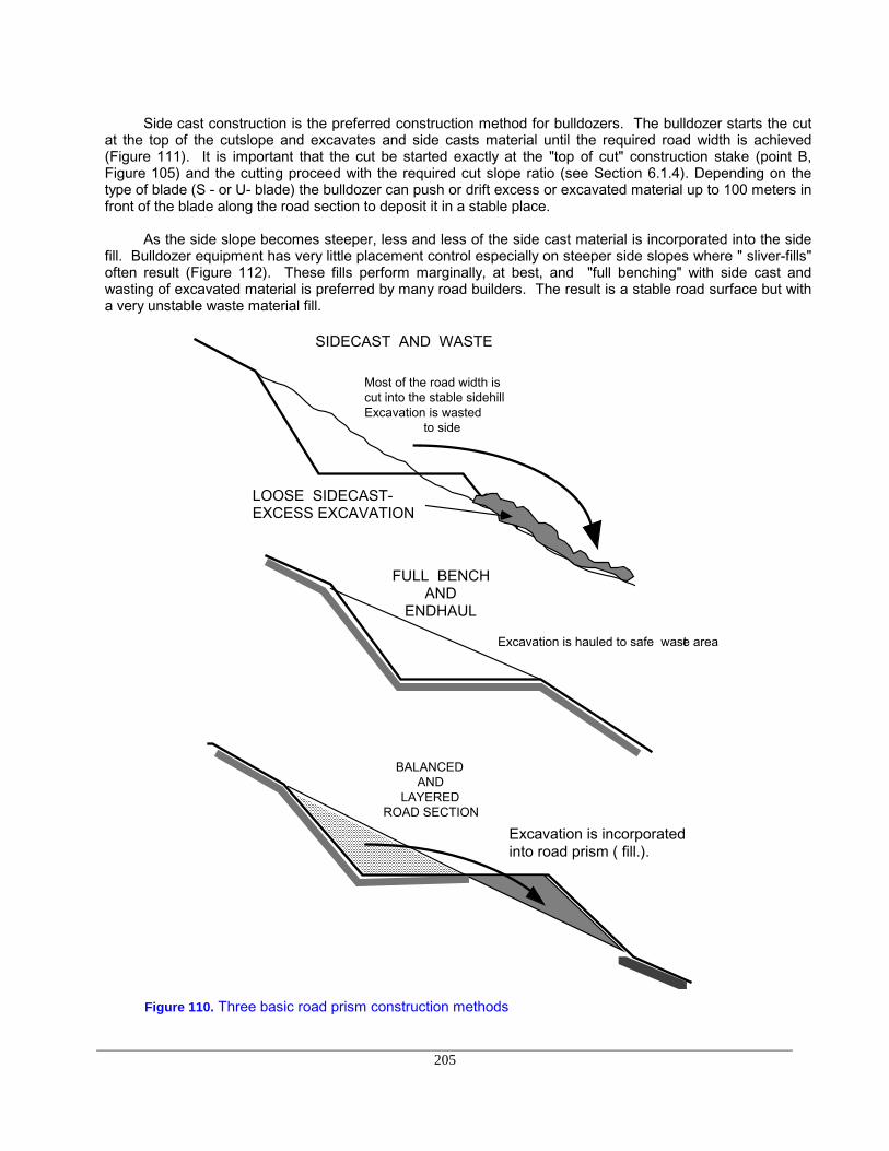
205

Side cast construction is the preferred construction method for bulldozers. The bulldozer starts the cutat the top of the cutslope and excavates and side casts material until the required road width is achieved(Figure 111). It is important that the cut be started exactly at the "top of cut" construction stake (point B,Figure 105) and the cutting proceed with the required cut slope ratio (see Section 6.1.4). Depending on thetype of blade (S - or U- blade) the bulldozer can push or drift excess or excavated material up to 100 meters infront of the blade along the road section to deposit it in a stable place.

As the side slope becomes steeper, less and less of the side cast material is incorporated into the sidefill. Bulldozer equipment has very little placement control especially on steeper side slopes where " sliver-fills"often result (Figure 112). These fills perform marginally, at best, and "full benching" with side cast andwasting of excavated material is preferred by many road builders. The result is a stable road surface but witha very unstable waste material fill.

SIDECAST AND WASTE

Most of the road width is cut into the stable sidehill Excavation is wasted to side

LOOSE SIDECAST- EXCESS EXCAVATION

FULL BENCH AND

ENDHAUL

Excavation is hauled to safe waste area

BALANCED AND

LAYERED ROAD SECTION

Excavation is incorporated into road prism ( fill.).

Figure 110. Three basic road prism construction methods

206

HILL SIDE WITH TOP OF CUT MARKED

1

2

EXCAVATION BY SIDECASTING

3

4

FINAL ROAD WIDTH

PIONEER ROAD

Figure 111. Road construction with a bulldozer; The machine starts at the top and in successivepasses excavates down to the required grade. Excavated material is side cast and mayform part of the roadway.

207

< 7o> 6 m

SLIVER FI LL

Figure 112. Sliver fills created on steep side slopes where ground slope and fill slope angles differ byless than 7o and fill slope height greater than 6.0 meters are inherently unstable.

Side cast or wasted material cannot remain stable on side slopes exceeding 60 to 70 percent. Undersuch conditions excavated material has to be end hauled to a safe disposal area. This requires dump trucksand excavators or shovels for loading and hauling.

Unwanted side cast may result from dozer excavation on steep side slopes because of lack ofplacement control. In order to contain side cast loss within the construction width of a full bench road the so-called "trench-method" has been successfully used in the Pacific Northwest (Nagygyor, 1984). In this methodthe right-of-way timber is felled parallel to the road centerline. Trees and stumps are not removed. They willact as a temporary retaining wall for loose, excavated material (Figure 113). A pioneer road is built at the topof the cut by drifting material against and on top of the felled trees. Initial excavation and side cast loss cantherefore be kept to a minimum. When rock is encountered, dirt drifted against or on top of trees will form atemporary bridge to allow passage of construction equipment.

Actual excavation is started about 10 to 12 meters from the loader by cutting a blade-wide trench anddrifting the material towards it. Loose material which escapes during this process is caught by the felled treesand slash. As the cut gets deeper material will fall inside the trench from both sides (Figure 113). Debris,stumps, tops and branches are pushed and loaded together with the excavated material,if it is not placed indesignated fills. Otherwise it can be separated out at this point.

208

TREES FELLED PARALLEL TO ROAD. ACT AS TEMPORARY RETAINING WALL

1st pass: Debris is caught by logs and stumps

2nd pass: Debris falls into trench

1

2

TRENCH CUT

STUMP

FELLED TREE

Figure 113. Trench-excavation to minimize sidehill loss of excavation material. Debris and materialfalls into trench in front of the dozer blade. Felled trees and stumps are left to act astemporary retaining walls until removed during final excavation.

6.3.2 Fill Construction

Fill construction is required to cross draws, creeks, flats or swampy areas and when excess excavationhas taken place. Road fills support traffic and therefore must withstand considerable abuse. Only mineralsoil, free of organic debris such as stumps, tree tops and humus should be used. Fills should be constructedand built up in layers (Figure 114). Each layer, or lift, should be spread and then compacted. Lift heightbefore compaction depends on the compaction equipment being used. Typically lift height should be about 30cm and should not exceed 50 cm. A bulldozer is not a good machine for compacting fills because of their lowground pressure characteristics. Fills across draws or creeks are especially critical since they may act asdams if the culvert should plug up. It is considered poor practice to build fills by end dumping instead oflayering and compacting (Figure 115).

209

COMPACTED LIFTS

30 - 50 cm

REMOVE VEGETATION AND ORGANIC DEBRIS

Figure 114. Fills are constructed by layering and compacting each layer. Lift height should notexceed 50 cm. Compaction should be done with proper compaction equipment and not abulldozer (from OSU Ext. Service 1983).

ROAD SURFACE

Figure 115. Fills that are part of the roadway should not be constructed by end dumping. (from OSUExt. Service, 1983).

210

6.3.3 Compaction

Proper compaction techniques result in significant cost reduction and reductions in erosion. Erosionpotential is directly proportional to the excavation volume especially if it is side cast in unconsolidated andloose fills. Conventional side cast techniques where most of the road surface is excavated into a stable hillside results in approximately 25 to 35 percent more excavated material when compared to "balanced" roaddesign and construction where the excavation is incorporated into the road prism. In the former case, most ifnot all of the excavated material is wasted as loose side cast material readily available for erosion. In thelatter case, it has been incorporated into the fill, properly compacted, and presumably unavailable for erosion.

The key to a stable, balanced road design is proper compaction of fill material. Haber and Koch (1982)quantified costs for erosion and compaction for several types of sediment control treatments on roads insouthwest Idaho. This study represents an excellent example of applying uniform criteria to examinedifferences between standard and non-standard construction techniques.

Costs were initially determined for each activity using two methods: (1) local (Boise) labor andequipment rates, taxes, insurance, and servicing (repair and maintenance) including 10 percent profit and riskmargin, and (2) Regional Equipment Blue Book Guidebook which include margins for profit and risk, fuel,oil,lubrication, repairs, maintenance, insurance, and incidental expenses. After actual costs for each activitywere calculated, average cost per unit and average crew cost was determined based on design quantities. Acomparison was then made between actual costs for "non-standard" treatments and actual costs of standardtreatments.

Average observed production rates for all activities were calculated for use in predicting time and costsassociated with "non-standard" construction techniques. Figure 116 illustrates an example of their results indetermining the cost of three different methods of embankment placement. These methods are: (1) side castembankments with no compactive effort, (2) layer placed (less than 30 cm (12 in) thick) embankments inwhich each layer is leveled and smoothed before each subsequent layer is placed (some compaction isobtained during the leveling process as the bulldozer passes over the material), and (3) controlled compactionin which embankments are placed in layers (less than 20 cm (8 in) thick) followed by compaction with waterand vibratory roller to achieve relative density of 95 percent.

As expected, side cast embankment construction per volume costs the least and controlled compactionthe most. (Road 106781 was shorter and only a small quantity of earth was moved resulting in a higher unitcost.) Total cost, however, for a road expressed in cost per unit length may be very similar for side castembankment and layered placement considering the fact that total excavation volume may be up to 35percent less for the latter case. As mentioned before, most of this excavated material is now consolidatedrather than loose. Combined with proper fill slope surface treatment and filter windrows very little erosion canbe expected.

It is worth noting that production rates of manual labor for excavation work are generally 3.8 to 4 m3 (5yd.3) of dirt during eight hours of work (Sheng,1977). However, these rates will vary widely depending onterrain, soil, environmental, and psychological conditions of the work crew.

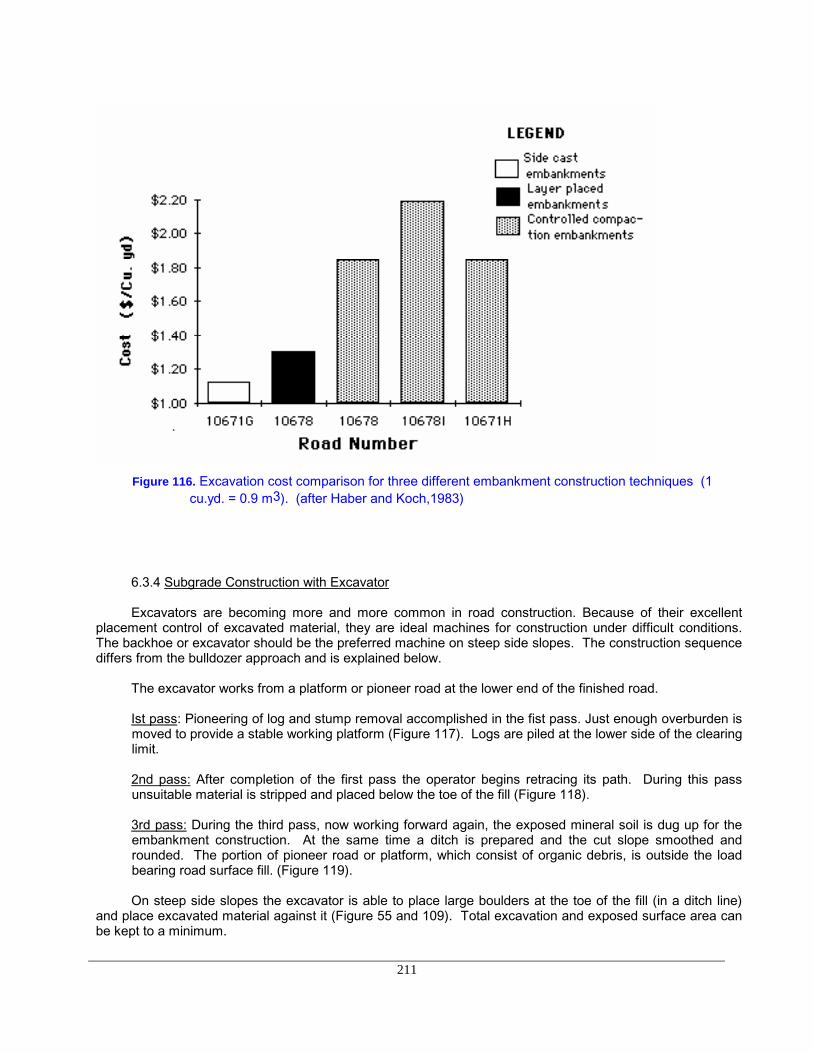
211

Figure 116. Excavation cost comparison for three different embankment construction techniques (1cu.yd. = 0.9 m3). (after Haber and Koch,1983)

6.3.4 Subgrade Construction with Excavator

Excavators are becoming more and more common in road construction. Because of their excellentplacement control of excavated material, they are ideal machines for construction under difficult conditions.The backhoe or excavator should be the preferred machine on steep side slopes. The construction sequencediffers from the bulldozer approach and is explained below.

The excavator works from a platform or pioneer road at the lower end of the finished road.

Ist pass: Pioneering of log and stump removal accomplished in the fist pass. Just enough overburden ismoved to provide a stable working platform (Figure 117). Logs are piled at the lower side of the clearinglimit.

2nd pass: After completion of the first pass the operator begins retracing its path. During this passunsuitable material is stripped and placed below the toe of the fill (Figure 118).

3rd pass: During the third pass, now working forward again, the exposed mineral soil is dug up for theembankment construction. At the same time a ditch is prepared and the cut slope smoothed androunded. The portion of pioneer road or platform, which consist of organic debris, is outside the loadbearing road surface fill. (Figure 119).

On steep side slopes the excavator is able to place large boulders at the toe of the fill (in a ditch line)and place excavated material against it (Figure 55 and 109). Total excavation and exposed surface area canbe kept to a minimum.

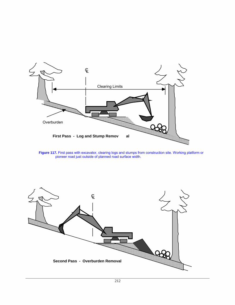
212

CL

Clearing Limits

Overburden

First Pass - Log and Stump Remov al

Figure 117. First pass with excavator, clearing logs and stumps from construction site. Working platform orpioneer road just outside of planned road surface width.

CL

Second Pass - Overburden Removal

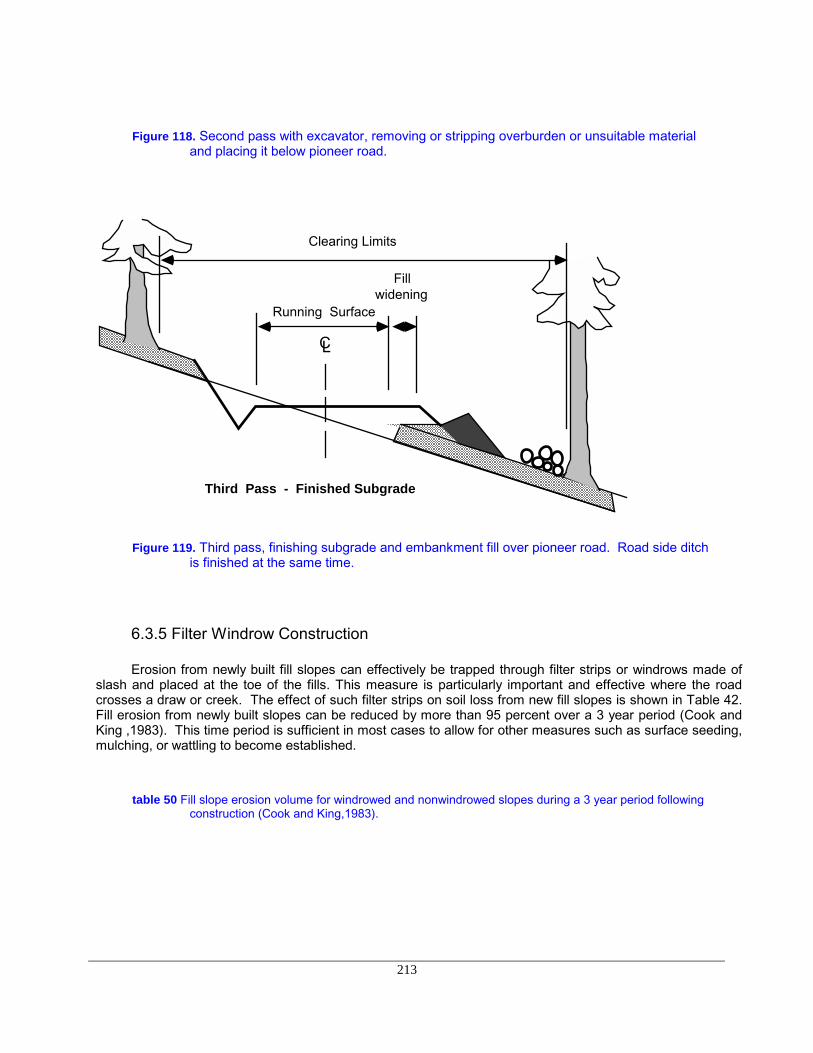
213

Figure 118. Second pass with excavator, removing or stripping overburden or unsuitable materialand placing it below pioneer road.

CL

Running Surface

Fill widening

Third Pass - Finished Subgrade

Clearing Limits

Figure 119. Third pass, finishing subgrade and embankment fill over pioneer road. Road side ditchis finished at the same time.

6.3.5 Filter Windrow Construction

Erosion from newly built fill slopes can effectively be trapped through filter strips or windrows made ofslash and placed at the toe of the fills. This measure is particularly important and effective where the roadcrosses a draw or creek. The effect of such filter strips on soil loss from new fill slopes is shown in Table 42.Fill erosion from newly built slopes can be reduced by more than 95 percent over a 3 year period (Cook andKing ,1983). This time period is sufficient in most cases to allow for other measures such as surface seeding,mulching, or wattling to become established.

table 50 Fill slope erosion volume for windrowed and nonwindrowed slopes during a 3 year period followingconstruction (Cook and King,1983).

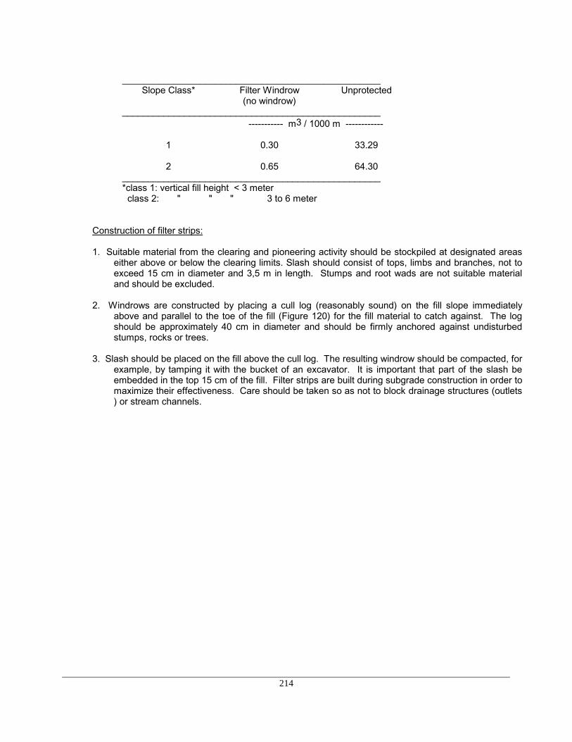
214

__________________________________________________Slope Class* Filter Windrow Unprotected

(no windrow)__________________________________________________

----------- m3 / 1000 m ------------

1 0.30 33.29

2 0.65 64.30__________________________________________________*class 1: vertical fill height < 3 meter class 2: " " " 3 to 6 meter

Construction of filter strips:

1. Suitable material from the clearing and pioneering activity should be stockpiled at designated areaseither above or below the clearing limits. Slash should consist of tops, limbs and branches, not toexceed 15 cm in diameter and 3,5 m in length. Stumps and root wads are not suitable materialand should be excluded.

2. Windrows are constructed by placing a cull log (reasonably sound) on the fill slope immediatelyabove and parallel to the toe of the fill (Figure 120) for the fill material to catch against. The logshould be approximately 40 cm in diameter and should be firmly anchored against undisturbedstumps, rocks or trees.

3. Slash should be placed on the fill above the cull log. The resulting windrow should be compacted, forexample, by tamping it with the bucket of an excavator. It is important that part of the slash beembedded in the top 15 cm of the fill. Filter strips are built during subgrade construction in order tomaximize their effectiveness. Care should be taken so as not to block drainage structures (outlets) or stream channels.

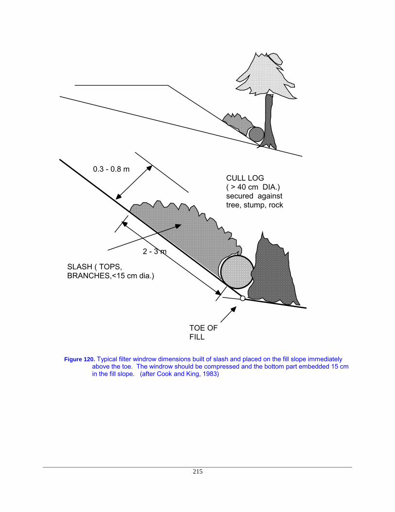
215

CULL LOG ( > 40 cm DIA.) secured against tree, stump, rock

0.3 - 0.8 m

2 - 3 m

SLASH ( TOPS, BRANCHES,<15 cm dia.)

TOE OF FILL

Figure 120. Typical filter windrow dimensions built of slash and placed on the fill slope immediatelyabove the toe. The windrow should be compressed and the bottom part embedded 15 cmin the fill slope. (after Cook and King, 1983)

216

LITERATURE CITED

Caterpillar. 1984. Caterpillar Performance Handbook, No. 14. Peoria, Illinois.

Cook, M.J. and J.G. King,1983. Construction cost and erosion control effectiveness of filter windrows on fillslopes. USDA Forest Service, Research Note INT-335, November 1983.

Dietz, P., W. Knigge and H. Loeffler. 1984. Walderschliessung. Verlag Paul Parey, Hamburg and Berlin,Germany.

Haber, D. and T. Koch. 1983. Costs of erosion control construction measures used on a forest road in theSilver Creek watershed in Idaho. U.S. Forest Service, Region 1 and University of Idaho, Moscow,Idaho.

Nagygyor, S.A. 1984. Construction of environmentally sound forest roads in the Pacific Northwest. In (edCorcoran and Gill) C.O.F.E./U.F.R.O. Proceedings, University of Maine, Orono, and University of NewBrunswick, Fredericton, April 1984, p.143 - 147.

Oregon State University. 1983. Road construction on woodland properties. Or. St. Univ. Ext. Cir. 1135.Corvallis, Oregon. 24 p.

Pearce, J. K. 1960. Forest Engineering Handbook. US Dept. of Interior. Bureau of Land Management. 220p.