
Real Business Cycle Theory -...
52
Real Business Cycle Theory Guido Ascari University of Pavia () Real Business Cycle Theory 1 / 50
Transcript of Real Business Cycle Theory -...
Real Business Cycle Theory
Guido Ascari
University of Pavia () Real Business Cycle Theory 1 / 50
Outline
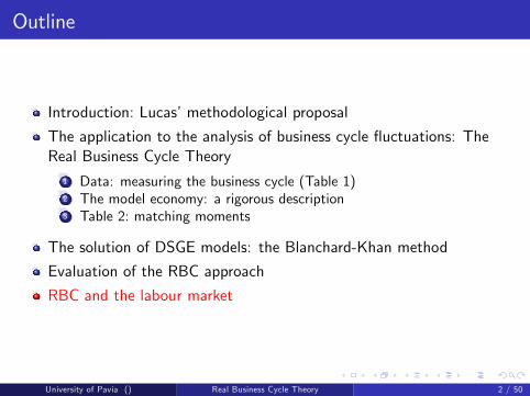
Introduction: Lucas�methodological proposal
The application to the analysis of business cycle �uctuations: TheReal Business Cycle Theory
1 Data: measuring the business cycle (Table 1)2 The model economy: a rigorous description3 Table 2: matching moments
The solution of DSGE models: the Blanchard-Khan method
Evaluation of the RBC approach
RBC and the labour market
University of Pavia () Real Business Cycle Theory 2 / 50
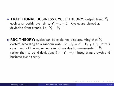
TRADITIONAL BUSINESS CYCLE THEORY: output trend Ytevolves smoothly over time, Yt = a+ bt. Cycles are viewed asdeviation from trends, i.e. Yt � Yt
RBC THEORY: cycles can be explained also assuming that Ytevolves according to a random walk, i.e., Yt = b+ Yt�1 + ut . In thiscase much of the movements in Yt are due to movements in Ytrather then to trend deviations Yt � Yt => Integrating growth andbusiness cycle theory
University of Pavia () Real Business Cycle Theory 3 / 50
The Lucas Methodological Proposal
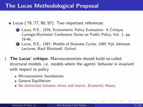
Lucas (�76,�77,�80,�87). Two important references:1 Lucas, R.E., 1976, Econometric Policy Evaluation: A Critique,Carnegie-Rochester Conference Series on Public Policy, Vol. 1, pp.19-46.
2 Lucas, R.E., 1987, Models of Business Cycles, 1985 Yrjö JahnssonLectures, Basil Blackwell, Oxford.
1. The Lucas�critique: Macroeconomists should build so-calledstructural models, i.e. models where the agents�behavior is invariantwith respect to policy
Microeconomic foundationsGeneral EquilibriumNo distinction between micro and macro: Economic theory
University of Pavia () Real Business Cycle Theory 4 / 50
2. Explicitly dynamic models from the outset:
Dynamic optimizationNeed for a theory of expectations formation => The RationalExpectations Revolution of the 1970s is the logical outcome of Lucas�research program
3. The Methodological Proposal
New analytical and computational instruments (Lucas/Stokey andPrescott, Kydland and Prescott)A new equilibrium concept: recursive equilibrium and "from a point to apath"Importance of expectations in the design of policy experimentsWelfare analysis
University of Pavia () Real Business Cycle Theory 5 / 50
CONCLUSIONS
Modern macroeconomics should employ dynamic general equilibriummodels (DSGE), that is, a macroeconomic model should be theresults of the solution of dynamic optimization problems underuncertainty by optimizing agents populating the model economy.
Build a "laboratory economy": much more di¢ cult task than oldKeynesian theorizing
Kydland & Prescott (1982) accepted the challenge posed by Lucas:they built the �rst Real Business Cycle (RBC) model.
University of Pavia () Real Business Cycle Theory 6 / 50
The basic RBC model in a nutshell
Outline of the RBC methodology:
a discrete-time stochastic model of the economy populated by maximizinghouseholds and �rms
MAIN SOURCE OF FLUCTUATIONS:
The erratic nature of technological progress
University of Pavia () Real Business Cycle Theory 7 / 50
THE BASIC MODEL: AS SIMPLE AS POSSIBLE
The Ramsey model of growth => integrating growth and cycle
All prices are �exible
All markets are walrasian
Rational expectations
No money
Endogenous labour
Technology shocks (and possibly other shocks) => stochastic steadystate
University of Pavia () Real Business Cycle Theory 8 / 50
MAIN RESULT AND FIRST INTUITION
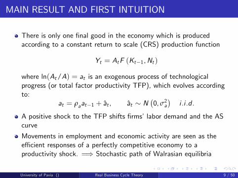
There is only one �nal good in the economy which is producedaccording to a constant return to scale (CRS) production function
Yt = AtF (Kt�1,Nt )
where ln(At/A) = at is an exogenous process of technologicalprogress (or total factor productivity TFP), which evolves accordingto:
at = ρaat�1 + at , at � N�0, σ2a
�i .i .d .
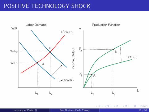
A positive shock to the TFP shifts �rms�labor demand and the AScurve
Movements in employment and economic activity are seen as thee¢ cient responses of a perfectly competitive economy to aproductivity shock. =) Stochastic path of Walrasian equilibria
University of Pavia () Real Business Cycle Theory 9 / 50
POSITIVE TECHNOLOGY SHOCK
University of Pavia () Real Business Cycle Theory 10 / 50
THE PLANNER PROBLEMRBC models do not consider any distortion or market imperfection,therefore the welfare theorems apply to these models:
1) the competitive equilibrium is pareto-optimal2) a pareto-optimal allocation can be decentralized as a competitiveequilibrium
The social planner equilibrium and the competitive equilibrium areidentical and admit a unique solution
University of Pavia () Real Business Cycle Theory 11 / 50

THE BASIC MODEL: AS SIMPLE AS POSSIBLE
Prescott did not think such a simple model could be of any use =>surprising result!
Main policy conclusion: �uctuations of all variable (output,consumption, employment, investment...) are the optimal responsesto technology shocks exogenous changes in the economicenvironment.
Shocks are not always desirable. But once they occur, this is the bestpossible outcome: business cycle �uctuations are the optimal responseto technology shocks => no need for government interventions: itcan be only deleterious
University of Pavia () Real Business Cycle Theory 12 / 50
Furious response from the "people from the Oceans" => Rogo¤:"brilliant theories �rst look ridiculous then they become obvious".
From mid�80s to mid�90s: ten years lost in useless ideological debatesbetween the Oceans and the Lakes
From mid�90s: convergence on methodology: "the RBC approach asthe new orthodoxy in macroeconomics"
University of Pavia () Real Business Cycle Theory 13 / 50
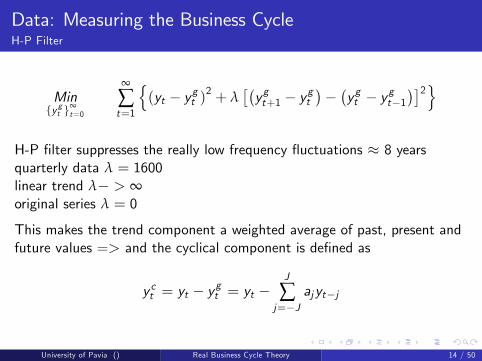
Data: Measuring the Business CycleH-P Filter
Minfy gt g
∞t=0
∞
∑t=1
n(yt � ygt )
2+ λ
��ygt+1 � y
gt���ygt � ygt�1
��2o
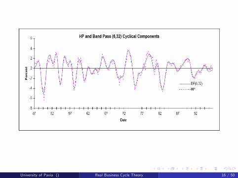
H-P �lter suppresses the really low frequency �uctuations � 8 yearsquarterly data λ = 1600linear trend λ� > ∞original series λ = 0
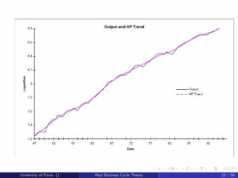
This makes the trend component a weighted average of past, present andfuture values => and the cyclical component is de�ned as
y ct = yt � ygt = yt �J
∑j=�J
ajyt�j
University of Pavia () Real Business Cycle Theory 14 / 50
University of Pavia () Real Business Cycle Theory 15 / 50
University of Pavia () Real Business Cycle Theory 16 / 50
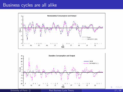
Business cycles are all alike
University of Pavia () Real Business Cycle Theory 17 / 50
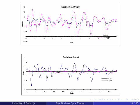
University of Pavia () Real Business Cycle Theory 18 / 50
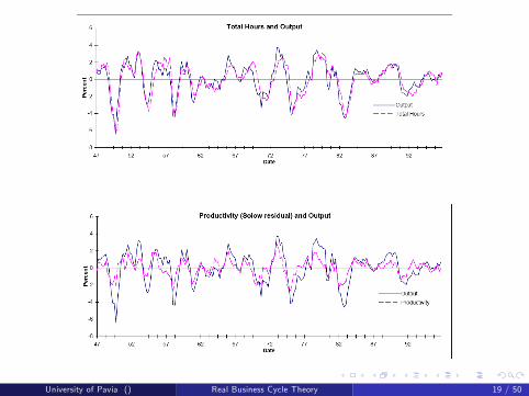
University of Pavia () Real Business Cycle Theory 19 / 50
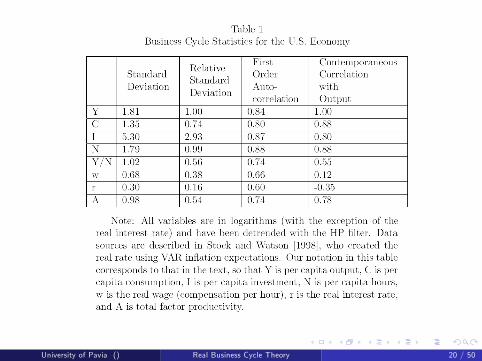
University of Pavia () Real Business Cycle Theory 20 / 50
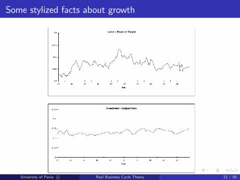
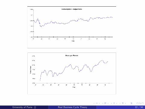
Some stylized facts about growth
University of Pavia () Real Business Cycle Theory 21 / 50
University of Pavia () Real Business Cycle Theory 22 / 50
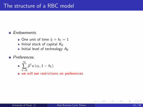
The structure of a RBC model
Endowments.
One unit of time lt + ht = 1Initial stock of capital K0Initial level of technology A0
Preferences.∞
∑t=0
βtu (ct , 1� ht )
we will see restrictions on preferences
University of Pavia () Real Business Cycle Theory 23 / 50
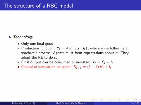
The structure of a RBC model
Technology.
Only one �nal goodProduction function: Yt = AtF (Kt ,Ht ) , where At is following astochastic process. Agents must form expectations about it. Theyadopt the RE to do so.Final output can be consumed or invested: Yt = Ct + ItCapital accumulation equation: Kt+1 = (1� δ)Kt + It
University of Pavia () Real Business Cycle Theory 24 / 50

The structure of a RBC model
Markets and Ownership.
Households are the owners of labor ht and capital kt , which they rentto �rms. Rental rates of labor and capital are: wt = Wt
Ptand rt .
Markets for inputs and output are competitive.The price of �nal output is normalized to 1.
University of Pavia () Real Business Cycle Theory 25 / 50
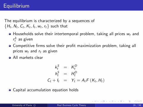
Equilibrium
The equilibrium is characterized by a sequences offHt ,Nt ,Ct ,Kt , It ,wt , rtg such that
Households solve their intertemporal problem, taking all prices wt andr kt as given
Competitive �rms solve their pro�t maximization problem, taking allprices wt and rt as given
All markets clear
kSt = KDthSt = HDt
Ct + It = Yt = AtF (Kt ,Ht )
Capital accumulation equation holds
University of Pavia () Real Business Cycle Theory 26 / 50
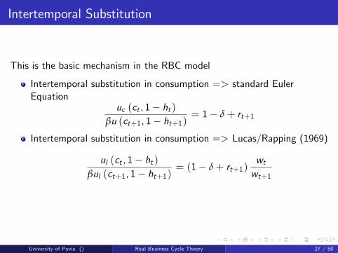
Intertemporal Substitution
This is the basic mechanism in the RBC model
Intertemporal substitution in consumption => standard EulerEquation
uc (ct , 1� ht )βu (ct+1, 1� ht+1)
= 1� δ+ rt+1
Intertemporal substitution in consumption => Lucas/Rapping (1969)
ul (ct , 1� ht )βul (ct+1, 1� ht+1)
= (1� δ+ rt+1)wtwt+1
University of Pavia () Real Business Cycle Theory 27 / 50
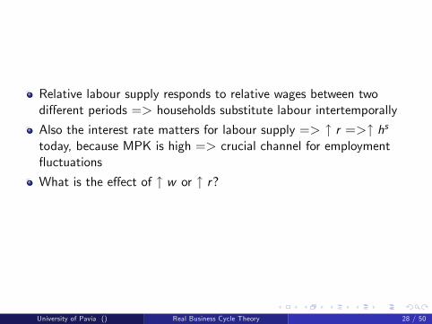
Relative labour supply responds to relative wages between twodi¤erent periods => households substitute labour intertemporally
Also the interest rate matters for labour supply => " r =>" hstoday, because MPK is high => crucial channel for employment�uctuations
What is the e¤ect of " w or " r?
University of Pavia () Real Business Cycle Theory 28 / 50
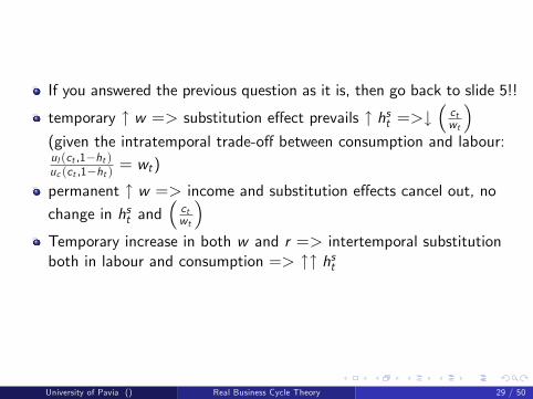
If you answered the previous question as it is, then go back to slide 5!!
temporary " w => substitution e¤ect prevails " hst =>#�ctwt
�(given the intratemporal trade-o¤ between consumption and labour:ul (ct ,1�ht )uc (ct ,1�ht ) = wt)
permanent " w => income and substitution e¤ects cancel out, no
change in hst and�ctwt
�Temporary increase in both w and r => intertemporal substitutionboth in labour and consumption => "" hst
University of Pavia () Real Business Cycle Theory 29 / 50
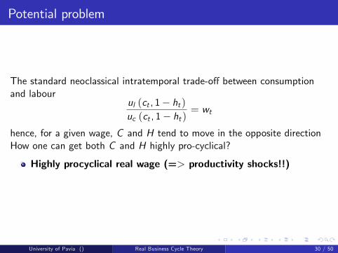
Potential problem
The standard neoclassical intratemporal trade-o¤ between consumptionand labour
ul (ct , 1� ht )uc (ct , 1� ht )
= wt
hence, for a given wage, C and H tend to move in the opposite directionHow one can get both C and H highly pro-cyclical?
Highly procyclical real wage (=> productivity shocks!!)
University of Pavia () Real Business Cycle Theory 30 / 50
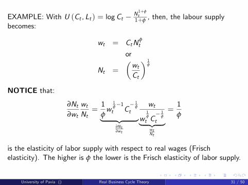
EXAMPLE: With U (Ct , Lt ) = logCt � N 1+φt1+φ , then, the labour supply
becomes:
wt = CtNφt
or
Nt =
�wtCt
� 1φ
NOTICE that:
∂Nt∂wt
wtNt=1φw
1φ�1t C
� 1φ
t| {z }∂Nt∂wt
wt
w1φ
t C� 1
φ
t| {z }wtNt
=1φ
is the elasticity of labor supply with respect to real wages (Frischelasticity). The higher is φ the lower is the Frisch elasticity of labor supply.
University of Pavia () Real Business Cycle Theory 31 / 50
Solution and numerical method
Next we will see in details an example taken from King, Plosser andRebelo (JME, 1988)
We will look at how to solve the model
from a theoretical perspective => Blanchard and Khan (Ecta, 1980)from a numerical perspective => simulation codes
University of Pavia () Real Business Cycle Theory 32 / 50
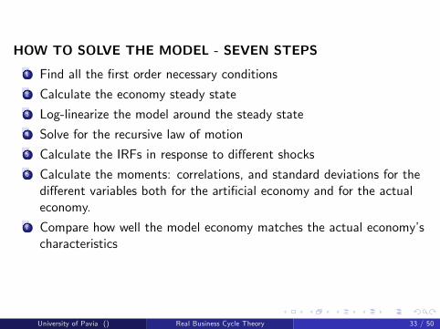
HOW TO SOLVE THE MODEL - SEVEN STEPS
1 Find all the �rst order necessary conditions2 Calculate the economy steady state3 Log-linearize the model around the steady state4 Solve for the recursive law of motion5 Calculate the IRFs in response to di¤erent shocks6 Calculate the moments: correlations, and standard deviations for thedi¤erent variables both for the arti�cial economy and for the actualeconomy.
7 Compare how well the model economy matches the actual economy�scharacteristics
University of Pavia () Real Business Cycle Theory 33 / 50
Simulation
We will see that
Productivity shocks are central. They need to be
LARGEPERSISTENTOTHER SHOCKS?
that�s because the internal propagation mechanism of the basic modelis weak (Cogley and Nason, AER, 1995)
University of Pavia () Real Business Cycle Theory 34 / 50
Before going to the example, the solution algorithm and the codes, let�sask ourselves:
IS THIS MODEL PROMISING?
University of Pavia () Real Business Cycle Theory 35 / 50
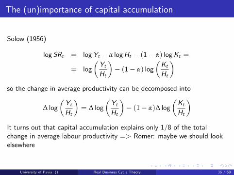
The (un)importance of capital accumulation
Solow (1956)
log SRt = logYt � α logHt � (1� α) logKt =
= log�YtHt
�� (1� α) log
�KtHt
�so the change in average productivity can be decomposed into
∆ log�YtHt
�= ∆ log
�YtHt
�� (1� α)∆ log
�KtHt
�It turns out that capital accumulation explains only 1/8 of the totalchange in average labour productivity => Romer: maybe we should lookelsewhere
University of Pavia () Real Business Cycle Theory 36 / 50
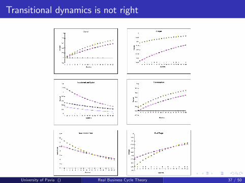
Transitional dynamics is not right
stars= basic RBC model; circles= �xed labour model; dashes in panel 3=labour response
University of Pavia () Real Business Cycle Theory 37 / 50
Go to �les:
notesRBC.pdf
detailmodel_matlab.pdf
University of Pavia () Real Business Cycle Theory 38 / 50
Criticism
Empirical philosophy: calibration vs. estimation
Too many parameters?Too much �exibility in choosing parameters? "The book of Ed"No possible statistical testing against alternativesis matching moments a desirable feature? econometrician aresuspicious of correlations
University of Pavia () Real Business Cycle Theory 39 / 50
Criticism
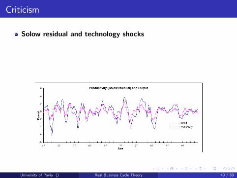
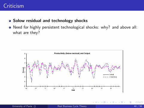
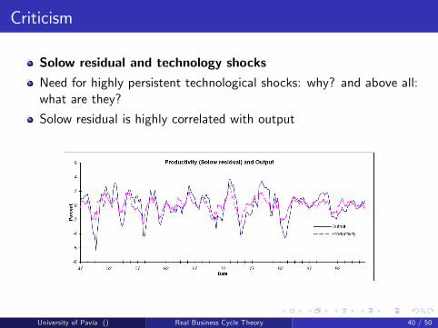
Solow residual and technology shocks
Need for highly persistent technological shocks: why? and above all:what are they?
Solow residual is highly correlated with output
University of Pavia () Real Business Cycle Theory 40 / 50
Criticism
Solow residual and technology shocksNeed for highly persistent technological shocks: why? and above all:what are they?
Solow residual is highly correlated with output
University of Pavia () Real Business Cycle Theory 40 / 50
Criticism
Solow residual and technology shocksNeed for highly persistent technological shocks: why? and above all:what are they?
Solow residual is highly correlated with output
University of Pavia () Real Business Cycle Theory 40 / 50
RBC View:
RBC theory argue that the strong correlation between output growthand Solow residuals is the evidence that productivity shocks are animportant source of economic �uctuations.
Critics:
Are economic �uctuations really caused by productivity shocks?
Expansions arise because of increases in productivity!. . . What does that mean about recessions? (Summers 1986)
It means that recessions are periods of technical regress! Burnside etal. estimates the probability of technological regress implied by SR tobe 37%!
Less implausible if supply shock considered more broadly (OPEC,strikes etc.)
University of Pavia () Real Business Cycle Theory 41 / 50
Real Achille�s heel: "measure of our ignorance"
Hall (1988): SR is useful to forecast military spending or othervariables that should not be a¤ected by technological shocks
Hall (1990): SR is mis-measured if there is imperfect competition,IRTS, or labour hoarding, or variable capacity utilization
Evans (1992):
money, interest rates and public spending Granger-cause SRa substantial component of σSR seems to be cause by aggregatedemand shocks
Bottom line: SR as measured out from a simple C-D production functionis very spurious
University of Pavia () Real Business Cycle Theory 42 / 50
Criticism
The Labour Market
Need for an highly elastic labour supply => labour market problemsThe increase in productivity translates to an increase in hours workedand to an increase in real wages. The e¤ect on the real wage isrelatively stronger the lower is the elasticity of labor supply 1
φ . In theextreme case of �xed labor supply all the increase in labor demandwould translate into an increase in the real wage.
CRITICS:
- labor supply does not depend that much on the intertemporal real wage;- high unemployment is mainly involuntary
University of Pavia () Real Business Cycle Theory 43 / 50
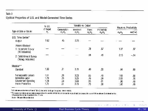
Hansen and Wright (FRBMQR, 1992)
Two problems:
σh > σw in the data, but not in the model
Fixer: Need for an highly elastic labour supply (Hansen, JME, 85)
corr(H,w) ' 0 in the data, close to 1 in the modelFixer: single shock problem (Christiano and Eichenbaum, AER, 92)
University of Pavia () Real Business Cycle Theory 44 / 50
University of Pavia () Real Business Cycle Theory 45 / 50
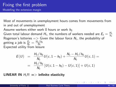
Fixing the �rst problemModelling the extensive margin
Most of movements in unemployment hours comes from movements fromin and out of unemploymentAssume workers either work 0 hours or work h0Given total labour demand Ht , the numbers of workers needed are Et = Ht
h0Rogerson�s lotteries => Given the labour force Nt , the probability ofgetting a job is EtNt =
Ht/h0Nt
Expected utility from leisure
E (U) =Ht/h0Nt
U(c , 1� h0) +Nt �Ht/h0
NtU(c , 1) =
=Ht/h0Nt
[U(c , 1� h0)� U(c , 1)] + U(c , 1)
LINEAR IN Ht !! => in�nite elasticity
University of Pavia () Real Business Cycle Theory 46 / 50
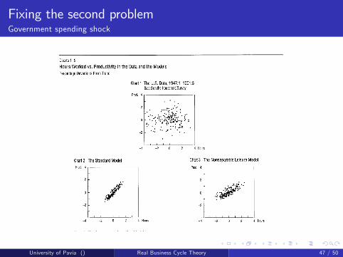
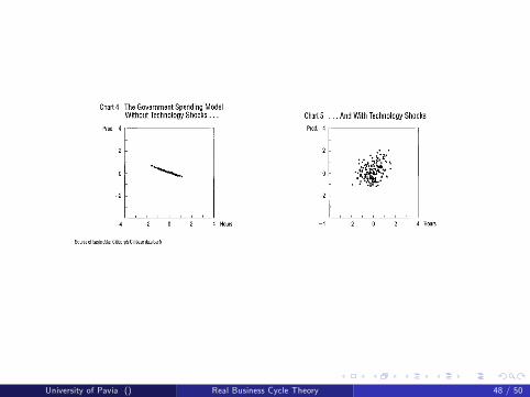
Fixing the second problemGovernment spending shock
University of Pavia () Real Business Cycle Theory 47 / 50
University of Pavia () Real Business Cycle Theory 48 / 50

Are wages and prices �exible?
RBC theory assumes that wages and prices are completely �exible, somarkets always clear.
RBC proponents argue that the degree of price stickiness occurring inthe real world is not important for understanding economic�uctuations.
They also assume �exible prices to be consistent with microeconomictheory.
Critics:
Wage and price stickiness explains involuntary unemployment and thenon-neutrality of money.
University of Pavia () Real Business Cycle Theory 49 / 50
SUMMING UP
Empirical signi�cance of intertemporal labor substitution mechanismis doubtful.
RBC theory implies that recessions are periods of technical regress!
Money is neutral so does not explain positive correlation betweenprices and output; and that this can be recti�ed by endogenizing themoney supply (Cooley and Hansen, AER, 1989)
Wage and price rigidity can help to explain involuntary unemploymentand non-neutrality of money
University of Pavia () Real Business Cycle Theory 50 / 50


