Eduardo Rossi University of...
92
GARCH Models Eduardo Rossi University of Pavia
Transcript of Eduardo Rossi University of...
GARCH Models
Eduardo Rossi
University of Pavia
Empirical regularities
Eduardo Rossi c© - Econometria mercati finanziari (avanzato) 2

Empirical regularities
Eduardo Rossi c© - Econometria mercati finanziari (avanzato) 3

Empirical regularities
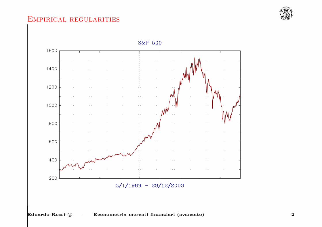
GARCH models have been developed to account for empirical
regularities in financial data. Many financial time series have a
number of characteristics in common.
• Asset prices are generally non stationary. Returns are usually
stationary. Some financial time series are fractionally integrated.
• Return series usually show no or little autocorrelation.
• Serial independence between the squared values of the series is
often rejected pointing towards the existence of non-linear
relationships between subsequent observations.
Eduardo Rossi c© - Econometria mercati finanziari (avanzato) 4
Empirical regularities
• Volatility of the return series appears to be clustered.
• Normality has to be rejected in favor of some thick-tailed
distribution.
• Some series exhibit so-called leverage effect, that is changes in
stock prices tend to be negatively correlated with changes in
volatility. A firm with debt and equity outstanding typically
becomes more highly leveraged when the value of the firm
falls.This raises equity returns volatility if returns are constant.
Black, however, argued that the response of stock volatility to the
direction of returns is too large to be explained by leverage alone.
• Volatilities of different securities very often move together.
Eduardo Rossi c© - Econometria mercati finanziari (avanzato) 5
Why do we need ARCH models?
Wold’s decomposition theorem establishes that any covariance
stationary {yt} may be written as the sum of a linearly deterministic
component and a linearly stochastic with a square-summable,
one-sided moving average representation. We can write,
yt = dt + ut
dt is linearly deterministic and ut is a linearly regular covariance
stationary stochastic process, given by
ut = B (L) εt
B (L) =∞∑
i=0
biLi
∞∑
i=0
b2i <∞ b0 = 1
Eduardo Rossi c© - Econometria mercati finanziari (avanzato) 6

Why do we need ARCH models?
E [εt] = 0
E [εtετ ] =
σ2ε <∞, if t = τ
0, otherwise
The uncorrelated innovation sequence need not to be Gaussian and
therefore need not be independent. Non-independent innovations are
characteristic of non-linear time series in general and conditionally
heteroskedastic time series in particular.
Eduardo Rossi c© - Econometria mercati finanziari (avanzato) 7

Why do we need ARCH models?
Now suppose that yt is a linear covariance stationary process with
i.i.d. innovations as opposed to merely white noise. The
unconditional mean and variance are
E [yt] = 0
E[
y2t
]
= σ2ε
∞∑
i=0
b2i
which are both invariant in time. The conditional mean is time
varying and is given by
E [yt |Φt−1 ] =∞∑
i=1
biεt−i
where the information set is Φt−1 = {εt−1, εt−2, . . .}.
Eduardo Rossi c© - Econometria mercati finanziari (avanzato) 8
Why do we need ARCH models?
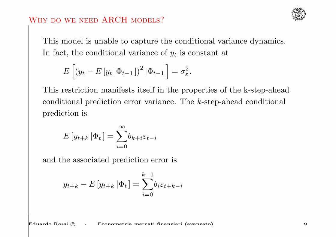
This model is unable to capture the conditional variance dynamics.
In fact, the conditional variance of yt is constant at
E[
(yt −E [yt |Φt−1 ])2|Φt−1
]
= σ2ε .
This restriction manifests itself in the properties of the k-step-ahead
conditional prediction error variance. The k -step-ahead conditional
prediction is
E [yt+k |Φt ] =∞∑
i=0
bk+iεt−i
and the associated prediction error is
yt+k − E [yt+k |Φt ] =k−1∑
i=0
biεt+k−i
Eduardo Rossi c© - Econometria mercati finanziari (avanzato) 9
Why do we need ARCH models?
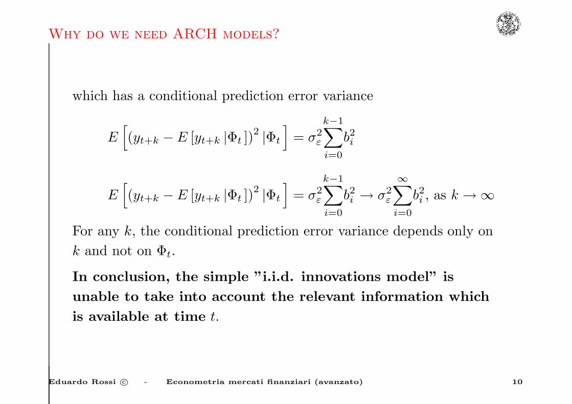
which has a conditional prediction error variance
E[
(yt+k − E [yt+k |Φt ])2|Φt
]
= σ2ε
k−1∑
i=0
b2i
E[
(yt+k − E [yt+k |Φt ])2|Φt
]
= σ2ε
k−1∑
i=0
b2i → σ2ε
∞∑
i=0
b2i , as k → ∞
For any k, the conditional prediction error variance depends only on
k and not on Φt.
In conclusion, the simple ”i.i.d. innovations model” is
unable to take into account the relevant information which
is available at time t.
Eduardo Rossi c© - Econometria mercati finanziari (avanzato) 10

The ARCH(q) Model
(Bollerslev, Engle and Nelson, 1994) The process {εt (θ0)} follows an
ARCH (AutoRegressive Conditional Heteroskedasticity) model if
Et−1 [εt (θ0)] = 0 t = 1, 2, . . . (1)
and the conditional variance
σ2t (θ0) ≡ V art−1 [εt (θ0)] = Et−1
[
ε2t (θ0)]
t = 1, 2, . . . (2)
depends non trivially on the σ-field generated by the past
observations: {εt−1 (θ0) , εt−2 (θ0) , . . .} .
Eduardo Rossi c© - Econometria mercati finanziari (avanzato) 11

The ARCH(q) Model
Let {yt (θ0)} denote the stochastic process of interest with
conditional mean
µt (θ0) ≡ Et−1 (yt) t = 1, 2, . . . (3)
µt (θ0) and σ2t (θ0) are measurable with respect to the time t− 1
information set. Define the {εt (θ0)} process by
εt (θ0) ≡ yt − µt (θ0) . (4)
Eduardo Rossi c© - Econometria mercati finanziari (avanzato) 12
The ARCH(q) Model
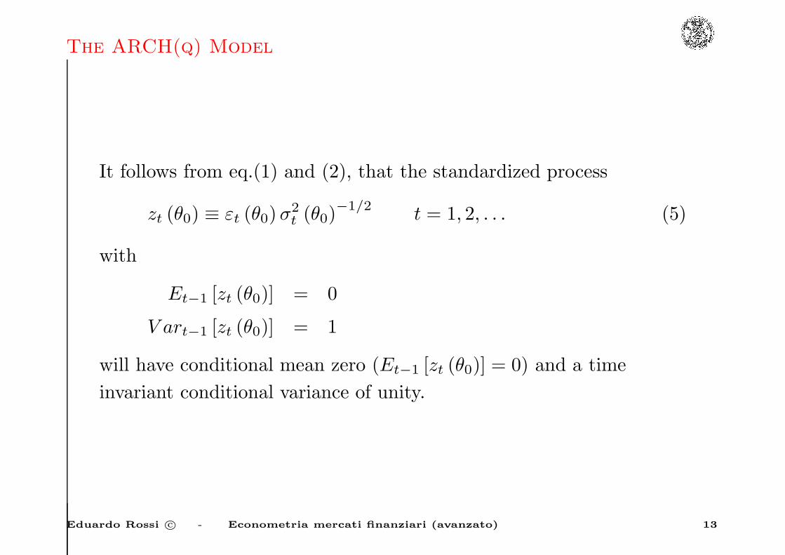
It follows from eq.(1) and (2), that the standardized process
zt (θ0) ≡ εt (θ0)σ2t (θ0)
−1/2 t = 1, 2, . . . (5)
with
Et−1 [zt (θ0)] = 0
V art−1 [zt (θ0)] = 1
will have conditional mean zero (Et−1 [zt (θ0)] = 0) and a time
invariant conditional variance of unity.
Eduardo Rossi c© - Econometria mercati finanziari (avanzato) 13

The ARCH(q) Model
We can think of εt (θ0) as generated by
εt (θ0) = zt (θ0)σ2t (θ0)
1/2
where ε2t (θ0) is unbiased estimator of σ2t (θ0).
Let’s suppose zt (θ0) ∼ NID (0, 1) and independent of σ2t (θ0)
Et−1
[
ε2t]
= Et−1
[
σ2t
]
Et−1
[
z2t
]
= Et−1
[
σ2t
]
= σ2t
because z2t |Φt−1 ∼ χ2
(1).
Eduardo Rossi c© - Econometria mercati finanziari (avanzato) 14

The ARCH(q) Model
If the conditional distribution of zt is time invariant with a finite
fourth moment, the fourth moment of εt is
E[
ε4t]
= E[
z4t
]
E[
σ4t
]
≥ E[
z4t
]
E[
σ2t
]2= E
[
z4t
]
E[
ε2t]2
where the last equality follows from
E[σ2t ] = E[Et−1(ε
2t )] = E[ε2t ]
E[
ε4t]
≥ E[
z4t
]
E[
ε2t]2
by Jensen’s inequality. The equality holds true for a constant
conditional variance only.
Eduardo Rossi c© - Econometria mercati finanziari (avanzato) 15
The ARCH(q) Model
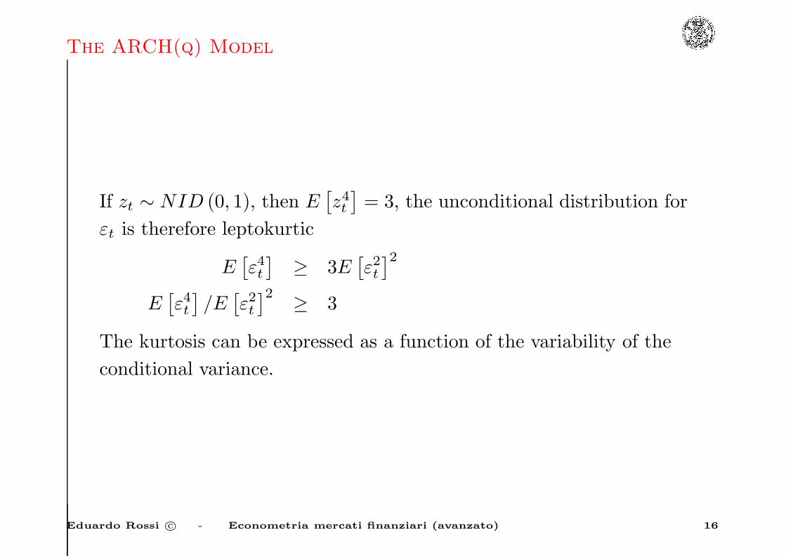
If zt ∼ NID (0, 1), then E[
z4t
]
= 3, the unconditional distribution for
εt is therefore leptokurtic
E[
ε4t]
≥ 3E[
ε2t]2
E[
ε4t]
/E[
ε2t]2
≥ 3
The kurtosis can be expressed as a function of the variability of the
conditional variance.
Eduardo Rossi c© - Econometria mercati finanziari (avanzato) 16

The ARCH(q) Model
In fact, if εt |Φt−1 ∼ N(
0, σ2t
)
Et−1
[
ε4t]
= 3Et−1
[
ε2t]2
E[
ε4t]
= 3E[
Et−1
(
ε2t)2]
≥ 3{
E[
Et−1
(
ε2t)]}2
= 3[
E(
ε2t)]2
E[
ε4t]
− 3[
E(
ε2t)]2
= 3E{
Et−1
[
ε2t]2}
− 3{
E[
Et−1
(
ε2t)]}2
E[
ε4t]
= 3[
E(
ε2t)]2
+ 3E{
Et−1
[
ε2t]2}
− 3{
E[
Et−1
(
ε2t)]}2
k =E[
ε4t]
[E (ε2t )]2 = 3 + 3
E{
Et−1
[
ε2t]2}
−{
E[
Et−1
(
ε2t)]}2
[E (ε2t )]2
= 3 + 3V ar
{
Et−1
[
ε2t]}
[E (ε2t )]2 = 3 + 3
V ar{
σ2t
}
[E (ε2t )]2 .
Eduardo Rossi c© - Econometria mercati finanziari (avanzato) 17
The ARCH(q) Model
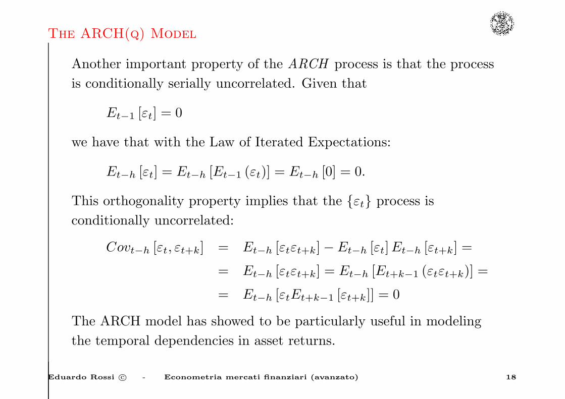
Another important property of the ARCH process is that the process
is conditionally serially uncorrelated. Given that
Et−1 [εt] = 0
we have that with the Law of Iterated Expectations:
Et−h [εt] = Et−h [Et−1 (εt)] = Et−h [0] = 0.
This orthogonality property implies that the {εt} process is
conditionally uncorrelated:
Covt−h [εt, εt+k] = Et−h [εtεt+k] −Et−h [εt]Et−h [εt+k] =
= Et−h [εtεt+k] = Et−h [Et+k−1 (εtεt+k)] =
= Et−h [εtEt+k−1 [εt+k]] = 0
The ARCH model has showed to be particularly useful in modeling
the temporal dependencies in asset returns.
Eduardo Rossi c© - Econometria mercati finanziari (avanzato) 18

The ARCH(q) Model
The ARCH (q) model introduced by Engle (Engle (1982)) is a linear
function of past squared disturbances:
σ2t = ω +
q∑
i=1
αiε2t−i (6)
In this model to assure a positive conditional variance the parameters
have to satisfy the following constraints: ω > 0 e
α1 ≥ 0, α2 ≥ 0, . . . , αq ≥ 0. Defining
σ2t ≡ ε2t − vt
where Et−1 (vt) = 0 we can write (6) as an AR(q) in ε2t :
ε2t = ω + α (L) ε2t + vt
where α (L) = α1L+ α2L2 + . . .+ αqL
q.
Eduardo Rossi c© - Econometria mercati finanziari (avanzato) 19

The ARCH(q) Model
(1 − α(L))ε2t = ω + vt
The process is weakly stationary if and only ifq∑
i=1
αi < 1; in this case
the unconditional variance is given by
E(
ε2t)
= ω/ (1 − α1 − . . .− αq) . (7)
Eduardo Rossi c© - Econometria mercati finanziari (avanzato) 20
The ARCH(q) Model
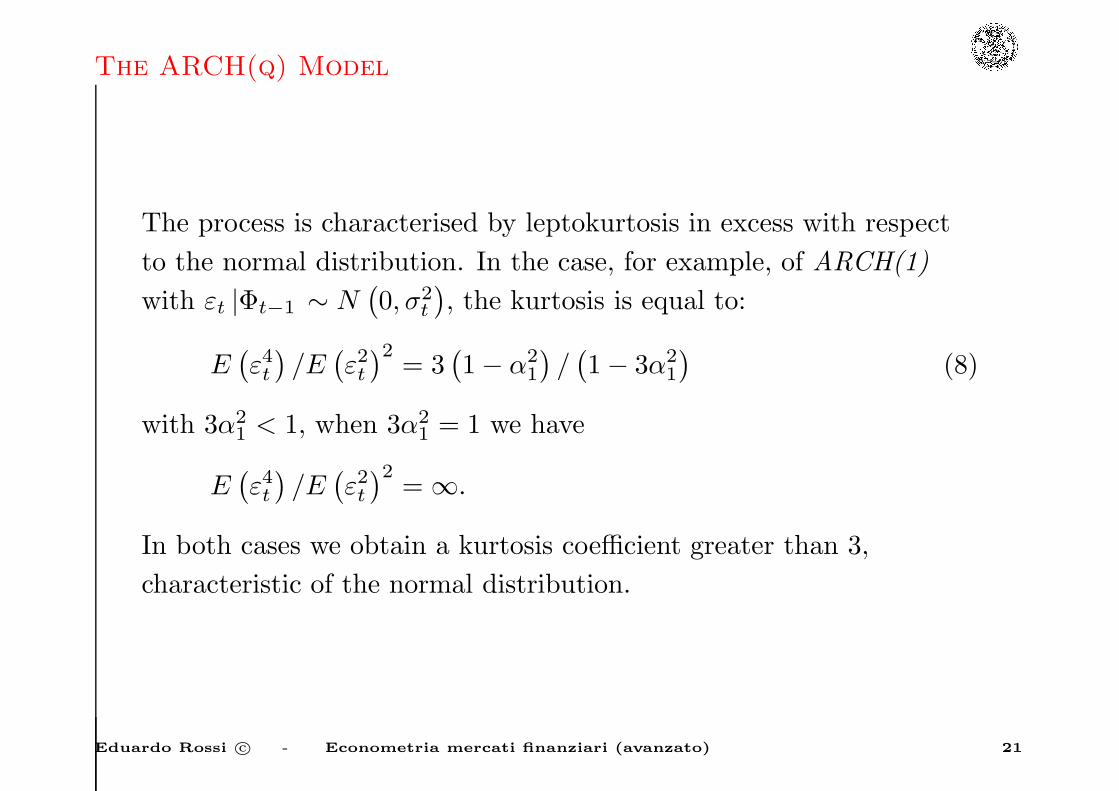
The process is characterised by leptokurtosis in excess with respect
to the normal distribution. In the case, for example, of ARCH(1)
with εt |Φt−1 ∼ N(
0, σ2t
)
, the kurtosis is equal to:
E(
ε4t)
/E(
ε2t)2
= 3(
1 − α21
)
/(
1 − 3α21
)
(8)
with 3α21 < 1, when 3α2
1 = 1 we have
E(
ε4t)
/E(
ε2t)2
= ∞.
In both cases we obtain a kurtosis coefficient greater than 3,
characteristic of the normal distribution.
Eduardo Rossi c© - Econometria mercati finanziari (avanzato) 21
The ARCH(q) Model
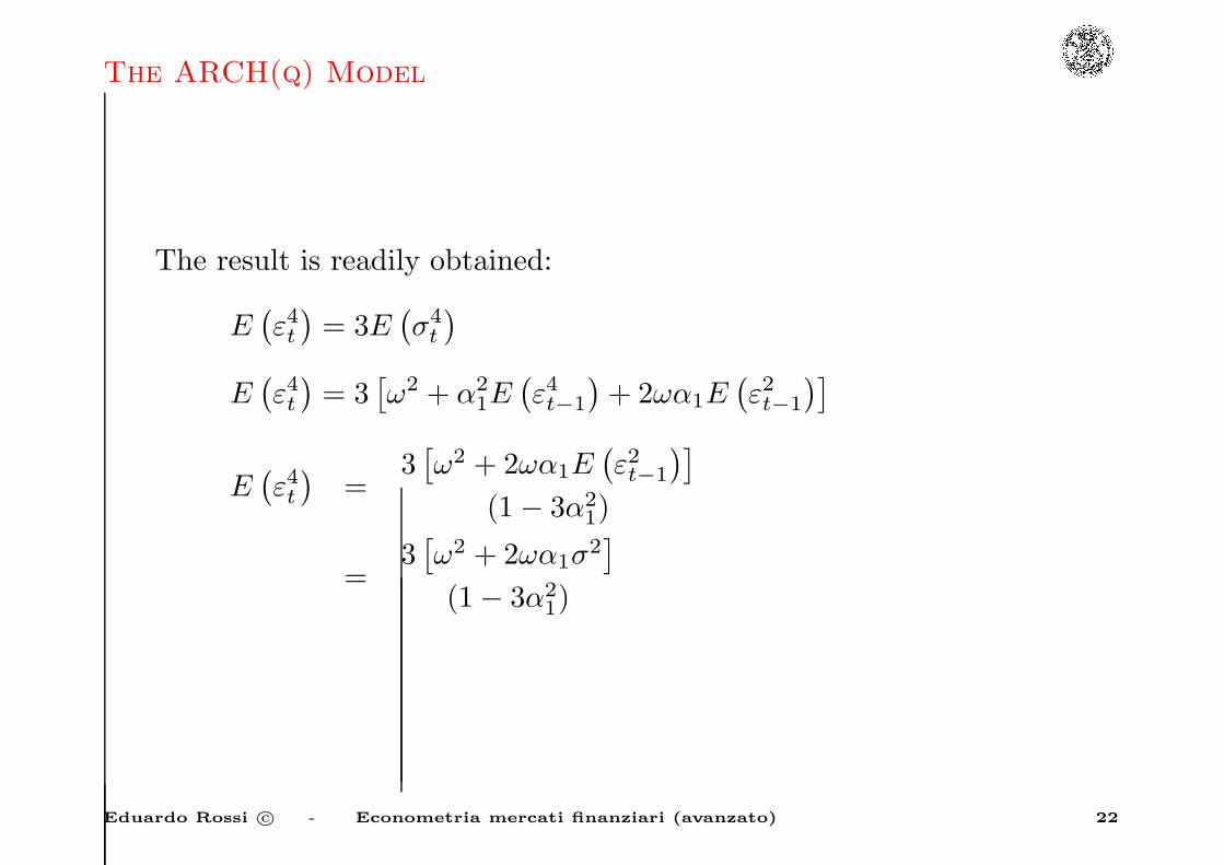
The result is readily obtained:
E(
ε4t)
= 3E(
σ4t
)
E(
ε4t)
= 3[
ω2 + α21E(
ε4t−1
)
+ 2ωα1E(
ε2t−1
)]
E(
ε4t)
=3[
ω2 + 2ωα1E(
ε2t−1
)]
(1 − 3α21)
=3[
ω2 + 2ωα1σ2]
(1 − 3α21)
Eduardo Rossi c© - Econometria mercati finanziari (avanzato) 22

The ARCH(q) Model
substituting σ2 = ω/ (1 − α1):
E(
ε4t)
=3[
ω2 (1 − α1) + 2ω2α1
]
(1 − 3α21) (1 − α1)
=3ω2 (1 + α1)
(1 − 3α21) (1 − α1)
finally
E(
ε4t)
/E(
ε2t)2
=3ω2 (1 + α1) (1 − α1)
2
(1 − 3α21) (1 − α1)ω2
=3(
1 − α21
)
1 − 3α21
. (9)
Eduardo Rossi c© - Econometria mercati finanziari (avanzato) 23
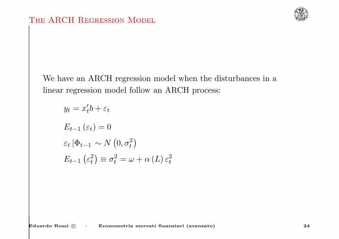
The ARCH Regression Model
We have an ARCH regression model when the disturbances in a
linear regression model follow an ARCH process:
yt = x′tb+ εt
Et−1 (εt) = 0
εt |Φt−1 ∼ N(
0, σ2t
)
Et−1
(
ε2t)
≡ σ2t = ω + α (L) ε2t
Eduardo Rossi c© - Econometria mercati finanziari (avanzato) 24

The GARCH(p,q) Model
In order to model in a parsimonious way the conditional
heteroskedasticity, Bollerslev (1986) proposed the Generalised ARCH
model, i.e GARCH(p,q):
σ2t = ω + α (L) ε2t + β (L)σ2
t . (10)
where α (L) = α1L+ . . .+ αqLq, β (L) = β1L+ . . .+ βpL
p.
The GARCH(1,1) is the most popular model in the empirical
literature:
σ2t = ω + α1ε
2t−1 + β1σ
2t−1. (11)
Eduardo Rossi c© - Econometria mercati finanziari (avanzato) 25

The GARCH(p,q) Model
To ensure that the conditional variance is well defined in a
GARCH (p,q) model all the coefficients in the corresponding linear
ARCH (∞) should be positive:
σ2t =
(
1 −
p∑
i=1
βiLi
)
−1
ω +
q∑
j=1
αjε2t−j
= ω∗ +∞∑
k=0
φkε2t−k−1 (12)
σ2t ≥ 0 if ω∗ ≥ 0 and all φk ≥ 0.
The non-negativity of ω∗ and φk is also a necessary condition for the
non negativity of σ2t .
Eduardo Rossi c© - Econometria mercati finanziari (avanzato) 26

The GARCH(p,q) Model
In order to make ω∗ e {φk}∞
k=0 well defined, assume that :
i. the roots of the polynomial β (x) = 1 lie outside the unit circle,
and that ω ≥ 0, this is a condition for ω∗ to be finite and positive.
ii. α (x) e 1 − β (x) have no common roots.
Eduardo Rossi c© - Econometria mercati finanziari (avanzato) 27

The GARCH(p,q) Model
These conditions are establishing nor that σ2t ≤ ∞ neither that
{
σ2t
}
∞
t=−∞is strictly stationary. For the simple GARCH(1,1) almost
sure positivity of σ2t requires, with the conditions (i) and (ii), that
(Nelson and Cao, 1992),
ω ≥ 0
β1 ≥ 0
α1 ≥ 0 (13)
Eduardo Rossi c© - Econometria mercati finanziari (avanzato) 28

The GARCH(p,q) Model
For the GARCH(1,q) and GARCH(2,q) models these constraints can
be relaxed, e.g. in the GARCH(1,2) model the necessary and
sufficient conditions become:
ω ≥ 0
0 ≤ β1 < 1
β1α1 + α2 ≥ 0
α1 ≥ 0 (14)
Eduardo Rossi c© - Econometria mercati finanziari (avanzato) 29
The GARCH(p,q) Model
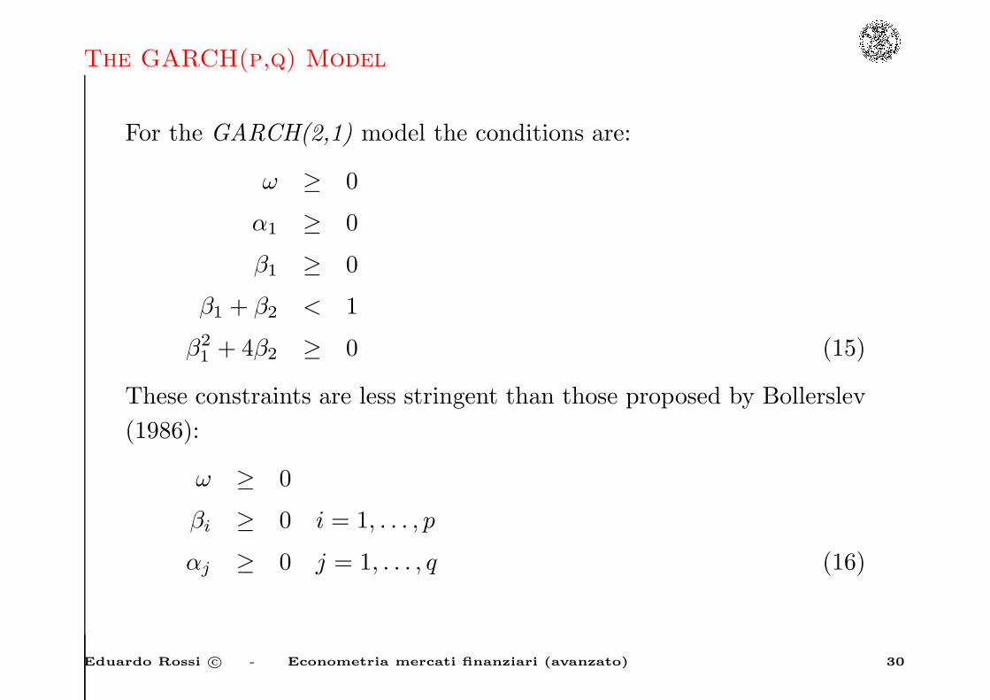
For the GARCH(2,1) model the conditions are:
ω ≥ 0
α1 ≥ 0
β1 ≥ 0
β1 + β2 < 1
β21 + 4β2 ≥ 0 (15)
These constraints are less stringent than those proposed by Bollerslev
(1986):
ω ≥ 0
βi ≥ 0 i = 1, . . . , p
αj ≥ 0 j = 1, . . . , q (16)
Eduardo Rossi c© - Econometria mercati finanziari (avanzato) 30
The GARCH(p,q) Model
These results cannot be adopted in the multivariate case, where the
requirement of positivity for{
σ2t
}
means the positive definiteness for
the conditional variance-covariance matrix.
Eduardo Rossi c© - Econometria mercati finanziari (avanzato) 31
The Yule-Walker equations for the squared process
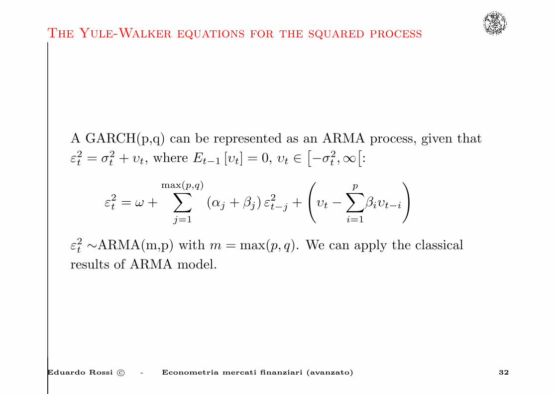
A GARCH(p,q) can be represented as an ARMA process, given that
ε2t = σ2t + υt, where Et−1 [υt] = 0, υt ∈
[
−σ2t ,∞
[
:
ε2t = ω +
max(p,q)∑
j=1
(αj + βj) ε2t−j +
(
υt −
p∑
i=1
βiυt−i
)
ε2t ∼ARMA(m,p) with m = max(p, q). We can apply the classical
results of ARMA model.
Eduardo Rossi c© - Econometria mercati finanziari (avanzato) 32

The Yule-Walker equations for the squared process
Example: GARCH(1,1)
σ2t = ω + α1ε
2t−1 + β1σ
2t−1
replacing σ2t with ε2t − υt, we obtain
ε2t − υt = ω + α1ε2t−1 + β1(ε
2t−1 − υt−1)
hence
ε2t = ω + (α1 + β1)ε2t−1 + υt − β1υt−1
Eduardo Rossi c© - Econometria mercati finanziari (avanzato) 33

The Yule-Walker equations for the squared process
We can study the autocovariance function, that is:
γ2 (k) = cov(
ε2t , ε2t−k
)
γ2 (k) = cov
ω +
m∑
j=1
(αj + βj) ε2t−j +
(
υt −
p∑
i=1
βiυt−i
)
, ǫ2t−k
γ2 (k) =
m∑
j=1
(αj + βj) cov(
ε2t−j , ε2t−k
)
+cov
[
υt −
p∑
i=1
βiυt−i, ε2t−k
]
(17)
When k is big enough, the last term on the right of expression (17) is
null.
Eduardo Rossi c© - Econometria mercati finanziari (avanzato) 34

The Yule-Walker equations for the squared process
The sequence of autocovariances satisfy a linear difference equation
of order max (p, q), for k ≥ p+ 1
γ2 (k) =
m∑
j=1
(αj + βj) γ2 (k − j)
This system can be used to identify the lag order m and p, that is the
p and q order if q ≥ p, the order p if q < p.
Eduardo Rossi c© - Econometria mercati finanziari (avanzato) 35
The GARCH Regression Model
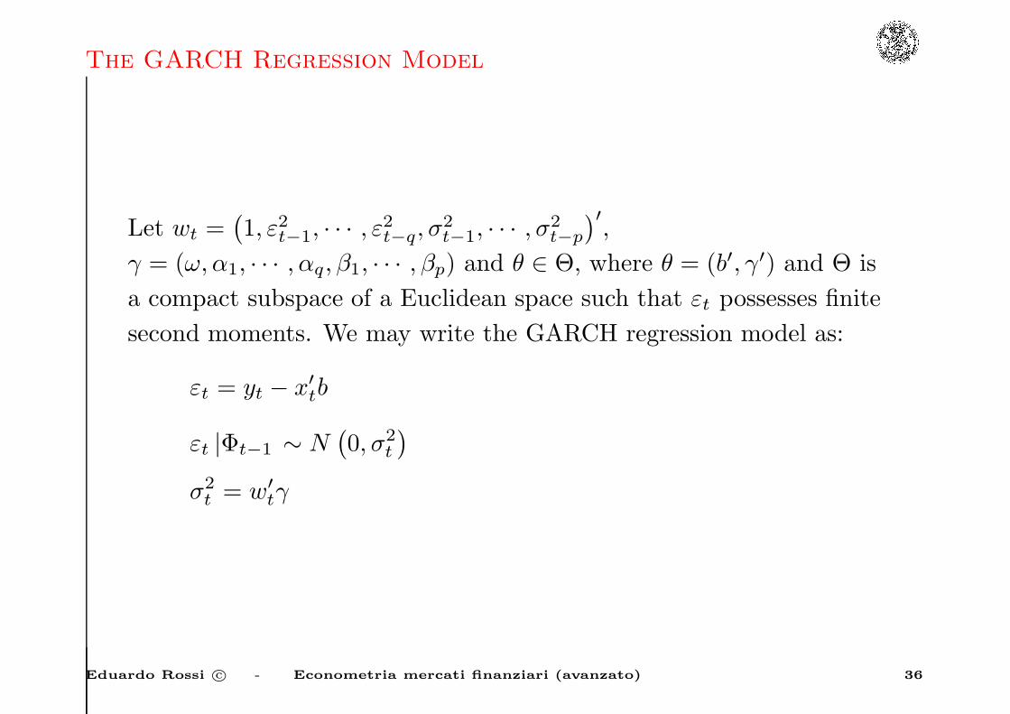
Let wt =(
1, ε2t−1, · · · , ε2t−q, σ
2t−1, · · · , σ
2t−p
)
′
,
γ = (ω, α1, · · · , αq, β1, · · · , βp) and θ ∈ Θ, where θ = (b′, γ′) and Θ is
a compact subspace of a Euclidean space such that εt possesses finite
second moments. We may write the GARCH regression model as:
εt = yt − x′tb
εt |Φt−1 ∼ N(
0, σ2t
)
σ2t = w′
tγ
Eduardo Rossi c© - Econometria mercati finanziari (avanzato) 36

Stationarity
The process {εt} which follows a GARCH(p,q) model is a martingale
difference sequence. In order to study second-order stationarity it’s
sufficient to consider that:
V ar [εt] = V ar [Et−1 (εt)] +E [V art−1 (εt)] = E[
σ2t
]
and show that is asymptotically constant in time (it does not depend
upon time).
A process {εt} which satisfies a GARCH(p,q) model with positive
coefficient ω ≥ 0, αi ≥ 0 i = 1, . . . , q, βi ≥ 0 i = 1, . . . , p is covariance
stationary if and only if:
α (1) + β(1) < 1
Eduardo Rossi c© - Econometria mercati finanziari (avanzato) 37

Stationarity
This is a sufficient but non necessary conditions for strict
stationarity. Because ARCH processes are thick tailed, the conditions
for covariance stationarity are often more stringent than the
conditions for strict stationarity.
A GARCH(1,1) model can be written as
σ2t = ω
[
1 +∞∑
k=1
k∏
i=1
(
β1 + α1z2t−i
)
]
Eduardo Rossi c© - Econometria mercati finanziari (avanzato) 38
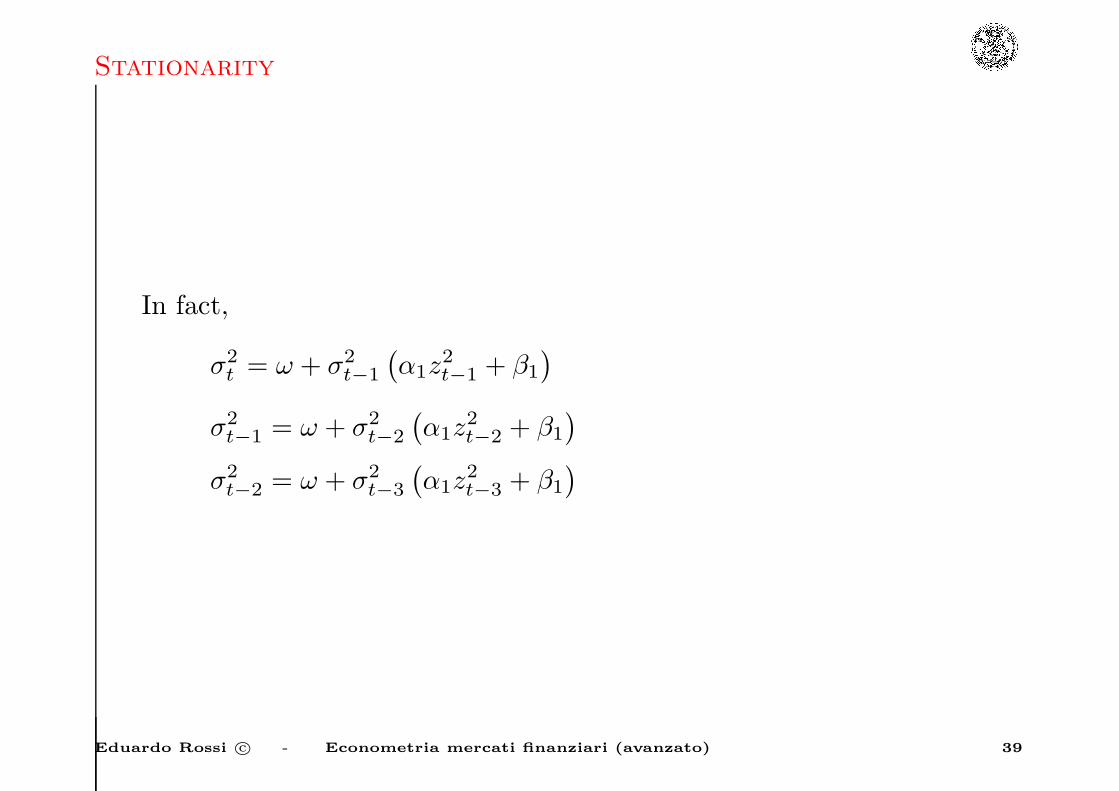
Stationarity
In fact,
σ2t = ω + σ2
t−1
(
α1z2t−1 + β1
)
σ2t−1 = ω + σ2
t−2
(
α1z2t−2 + β1
)
σ2t−2 = ω + σ2
t−3
(
α1z2t−3 + β1
)
Eduardo Rossi c© - Econometria mercati finanziari (avanzato) 39

Stationarity
σ2t = ω +
[
ω + σ2t−2
(
α1z2t−2 + β1
)] (
α1z2t−1 + β1
)
= ω + ω(
α1z2t−1 + β1
)
+ σ2t−2
(
α1z2t−2 + β1
) (
α1z2t−1 + β1
)
= ω + ω(
α1z2t−1 + β1
)
+ ω(
α1z2t−1 + β1
) (
α1z2t−2 + β1
)
+σ2t−3
(
α1z2t−3 + β1
) (
α1z2t−2 + β1
) (
α1z2t−1 + β1
)
finally,
σ2t = ω
[
1 +∞∑
k=1
k∏
i=1
(
α1z2t−i + β1
)
]
Eduardo Rossi c© - Econometria mercati finanziari (avanzato) 40

Stationarity
Nelson shows that when ω > 0, σ2t <∞ a.s. and
{
εt, σ2t
}
is strictly
stationary if and only if E[
ln(
β1 + α1z2t
)]
< 0
E[
ln(
β1 + α1z2t
)]
≤ ln[
E(
β1 + α1z2t
)]
= ln (α1 + β1)
when α1 + β1 = 1 the model is strictly stationary.
E[
ln(
β1 + α1z2t
)]
< 0 is a weaker requirement than α1 + β1 < 1.
Eduardo Rossi c© - Econometria mercati finanziari (avanzato) 41

Stationarity
Example
ARCH(1), with α1 = 1, β1 = 0, zt ∼ N (0, 1)
E[
ln(
z2t
)]
≤ ln[
E(
z2t
)]
= ln (1)
It’s strictly but not covariance stationary. The ARCH(q) is
covariance stationary if and only if the sum of the positive
parameters is less than one.
Eduardo Rossi c© - Econometria mercati finanziari (avanzato) 42

Forecasting volatility
Forecasting with a GARCH(p,q) (Engle and Bollerslev 1986):
σ2t+k = ω +
q∑
i=1
αiε2t+k−i +
p∑
i=1
βiσ2t+k−i
we can write the process in two parts, before and after time t:
σ2t+k = ω+
n∑
i=1
[
αiε2t+k−i + βiσ
2t+k−i
]
+m∑
i=k
[
αiε2t+k−i + βiσ
2t+k−i
]
where n = min {m, k − 1} and by definition summation from 1 to 0
and from k > m to m both are equal to zero.
Eduardo Rossi c© - Econometria mercati finanziari (avanzato) 43

Forecasting volatility
Thus
Et
[
σ2t+k
]
= ω+n∑
i=1
[
(αi + βi)Et
(
σ2t+k−i
)]
+m∑
i=k
[
αiε2t+k−i + βiσ
2t+k−i
]
.
Eduardo Rossi c© - Econometria mercati finanziari (avanzato) 44

Forecasting volatility
In particular for a GARCH(1,1) and k > 2:
Et
[
σ2t+k
]
=k−2∑
i=0
(α1 + β1)i ω + (α1 + β1)
k−1 σ2t+1
= ω
[
1 − (α1 + β1)k−1]
[1 − (α1 + β1)]+ (α1 + β1)
k−1 σ2t+1
= σ2[
1 − (α1 + β1)k−1]
+ (α1 + β1)k−1
σ2t+1
= σ2 + (α1 + β1)k−1 [
σ2t+1 − σ2
]
When the process is covariance stationary, it follows that Et
[
σ2t+k
]
converges to σ2 as k → ∞.
Eduardo Rossi c© - Econometria mercati finanziari (avanzato) 45

The IGARCH(p,q) model
The GARCH(p,q) process characterized by the first two conditional
moments:
Et−1 [εt] = 0
σ2t ≡ Et−1
[
ε2t]
= ω +
q∑
i=1
αiε2t−i +
p∑
i=1
βiσ2t−i
where ω ≥ 0, αi ≥ 0 and βi ≥ 0 for all i and the polynomial
1 − α (x) − β(x) = 0
has d > 0 unit root(s) and max {p, q} − d root(s) outside the unit
circle is said to be:
Eduardo Rossi c© - Econometria mercati finanziari (avanzato) 46
The IGARCH(p,q) model
• Integrated in variance of order d if ω = 0
• Integrated in variance of order d with trend if ω > 0.
The Integrated GARCH(p,q) models, both with or without trend, are
therefore part of a wider class of models with a property called
”persistent variance” in which the current information remains
important for the forecasts of the conditional variances for all horizon.
Eduardo Rossi c© - Econometria mercati finanziari (avanzato) 47

The IGARCH(p,q) model
So we have the Integrated GARCH(p,q) model when (necessary
condition)
α (1) + β(1) = 1
To illustrate consider the IGARCH(1,1) which is characterised by
α1 + β1 = 1
σ2t = ω + α1ε
2t−1 + (1 − α1)σ
2t−1
σ2t = ω + σ2
t−1 + α1
(
ε2t−1 − σ2t−1
)
0 < α1 ≤ 1
For this particular model the conditional variance k steps in the
future is:
Et
[
σ2t+k
]
= (k − 1)ω + σ2t+1
Eduardo Rossi c© - Econometria mercati finanziari (avanzato) 48

Persistence
• In many studies of the time series behavior of asset volatility the
question has been how long shocks to conditional variance persist.
• If volatility shocks persist indefinitely, they may move the whole
term structure of risk premia.
• There are many notions of convergence in the probability theory
(almost sure, in probability, in Lp), so whether a shock is
transitory or persistent may depend on the definition of
convergence.
Eduardo Rossi c© - Econometria mercati finanziari (avanzato) 49

Persistence
• In linear models it typically makes no difference which of the
standard definitions we use, since the definitions usually agree.
• In GARCH models the situation is more complicated.
In the IGARCH(1,1):
σ2t = ω + α1ε
2t−1 + β1σ
2t−1
where α1 + β1 = 1. Given that ε2t = z2t σ
2t , we can rewrite the
IGARCH(1,1) process as
σ2t = ω + σ2
t−1
[
(1 − α1) + α1z2t−1
]
0 < α1 ≤ 1.
When ω = 0, σ2t is a martingale.
Eduardo Rossi c© - Econometria mercati finanziari (avanzato) 50

Persistence
Based on the nature of persistence in linear models, it seems that
IGARCH(1,1) with ω > 0 and ω = 0 are analogous to random walks
with and without drift, respectively, and are therefore natural models
of ”persistent” shocks.
This turns out to be misleading, however:
• in IGARCH(1,1) with ω = 0, σ2t collapses to zero almost
surely
• in IGARCH(1,1) with ω > 0, σ2t is strictly stationary and ergodic
and therefore does not behave like a random walk, since random
walks diverge almost surely.
Eduardo Rossi c© - Econometria mercati finanziari (avanzato) 51

Persistence
Two notions of persistence.
1. Suppose σ2t is strictly stationary and ergodic. Let F
(
σ2t
)
be the
unconditional cdf for σ2t , and Fs
(
σ2t
)
the conditional cdf for σ2t ,
given information at time s < t. For any s F(
σ2t
)
− Fs
(
σ2t
)
→ 0
at all continuity points as t→ ∞. There is no persistence when{
σ2t
}
is stationary and ergodic.
2. Persistence is defined in terms of forecast moments. For some
η > 0, the shocks to σ2t fail to persist if and only if for every s,
Es
(
σ2ηt
)
converges, as t→ ∞, to a finite limit independent of
time s information set.
Eduardo Rossi c© - Econometria mercati finanziari (avanzato) 52

Persistence
Whether or not shocks to{
σ2t
}
”persist” depends very much on
which definition is adopted. The conditional moment may diverge to
infinity for some η, but converge to a well-behaved limit independent
of initial conditions for other η, even when the{
σ2t
}
is stationary and
ergodic.
Eduardo Rossi c© - Econometria mercati finanziari (avanzato) 53
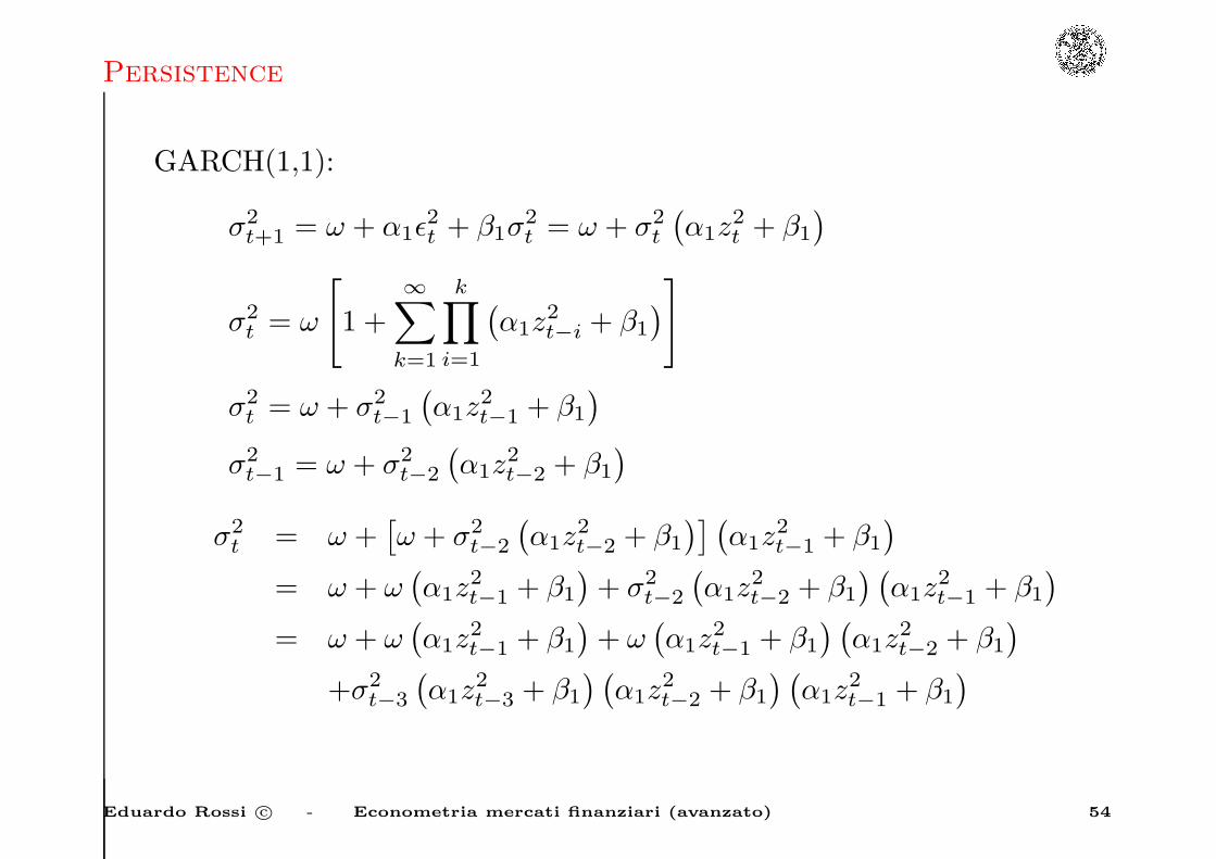
Persistence
GARCH(1,1):
σ2t+1 = ω + α1ǫ
2t + β1σ
2t = ω + σ2
t
(
α1z2t + β1
)
σ2t = ω
[
1 +∞∑
k=1
k∏
i=1
(
α1z2t−i + β1
)
]
σ2t = ω + σ2
t−1
(
α1z2t−1 + β1
)
σ2t−1 = ω + σ2
t−2
(
α1z2t−2 + β1
)
σ2t = ω +
[
ω + σ2t−2
(
α1z2t−2 + β1
)] (
α1z2t−1 + β1
)
= ω + ω(
α1z2t−1 + β1
)
+ σ2t−2
(
α1z2t−2 + β1
) (
α1z2t−1 + β1
)
= ω + ω(
α1z2t−1 + β1
)
+ ω(
α1z2t−1 + β1
) (
α1z2t−2 + β1
)
+σ2t−3
(
α1z2t−3 + β1
) (
α1z2t−2 + β1
) (
α1z2t−1 + β1
)
Eduardo Rossi c© - Econometria mercati finanziari (avanzato) 54
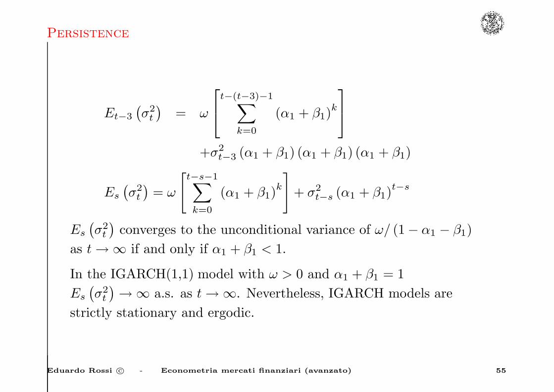
Persistence
Et−3
(
σ2t
)
= ω
t−(t−3)−1∑
k=0
(α1 + β1)k
+σ2t−3 (α1 + β1) (α1 + β1) (α1 + β1)
Es
(
σ2t
)
= ω
[
t−s−1∑
k=0
(α1 + β1)k
]
+ σ2t−s (α1 + β1)
t−s
Es
(
σ2t
)
converges to the unconditional variance of ω/ (1 − α1 − β1)
as t→ ∞ if and only if α1 + β1 < 1.
In the IGARCH(1,1) model with ω > 0 and α1 + β1 = 1
Es
(
σ2t
)
→ ∞ a.s. as t→ ∞. Nevertheless, IGARCH models are
strictly stationary and ergodic.
Eduardo Rossi c© - Econometria mercati finanziari (avanzato) 55
The EGARCH(p,q) Model
• GARCH models assume that only the magnitude and not the
positivity or negativity of unanticipated excess returns
determines feature σ2t .
• There exists a negative correlation between stock returns and
changes in returns volatility, i.e. volatility tends to rise in
response to ”bad news”, (excess returns lower than expected)
and to fall in response to ”good news” (excess returns higher
than expected).
Eduardo Rossi c© - Econometria mercati finanziari (avanzato) 56

The EGARCH(p,q) Model
If we write σ2t as a function of lagged σ2
t and lagged z2t , where
ε2t = z2t σ
2t
σ2t = ω +
q∑
j=1
αjz2t−jσ
2t−j +
p∑
i=1
βiσ2t−i
it is evident that the conditional variance is invariant to changes in
sign of the z′ts. Moreover, the innovations z2t−jσ
2t−j are not i.i.d.
• The nonnegativity constraints on ω∗ and φk, which are imposed
to ensure that σ2t remains nonnegative for all t with probability
one. These constraints imply that increasing z2t in any period
increases σ2t+m for all m ≥ 1, ruling out random oscillatory
behavior in the σ2t process.
Eduardo Rossi c© - Econometria mercati finanziari (avanzato) 57

The EGARCH(p,q) Model
• The GARCH models are not able to explain the observed
covariance between ε2t and εt−j . This is possible only if the
conditional variance is expressed as an asymmetric function of
εt−j .
• In GARCH(1,1) models, shocks may persist in one norm and die
out in another, so the conditional moments of GARCH(1,1) may
explode even when the process is strictly stationary and ergodic.
• GARCH models essentially specify the behavior of the square of
the data. In this case a few large observations can dominate the
sample.
Eduardo Rossi c© - Econometria mercati finanziari (avanzato) 58

The EGARCH(p,q) Model
In the EGARCH(p,q) model (Exponential GARCH(p,q)) put forward
by Nelson the σ2t depends on both size and the sign of lagged
residuals. This is the first example of asymmetric model:
ln(
σ2t
)
= ω +
p∑
i=1
βi ln(
σ2t−i
)
+
q∑
i=1
αi [φzt−i + ψ (|zt−i| −E |zt−i|)]
α1 ≡ 1, E |zt| = (2/π)1/2given that zt ∼ NID(0, 1), where the
parameters ω, βi, αi are not restricted to be nonnegative. Let define
g (zt) ≡ φzt + ψ [|zt| −E |zt|]
by construction {g (zt)}∞
t=−∞is a zero-mean, i.i.d. random sequence.
Eduardo Rossi c© - Econometria mercati finanziari (avanzato) 59
The EGARCH(p,q) Model
• The components of g (zt) are φzt and ψ [|zt| −E |zt|], each with
mean zero.
• If the distribution of zt is symmetric, the components are
orthogonal, but not independent.
• Over the range 0 < zt <∞, g (zt) is linear in zt with slope φ+ ψ,
and over the range −∞ < zt ≤ 0, g (zt) is linear with slope φ−ψ.
• The term ψ [|zt| −E |zt|] represents a magnitude effect.
Eduardo Rossi c© - Econometria mercati finanziari (avanzato) 60

The EGARCH(p,q) Model
• If ψ > 0 and φ = 0, the innovation in ln(
σ2t+1
)
is positive
(negative) when the magnitude of zt is larger (smaller) than its
expected value.
• If ψ = 0 and φ < 0, the innovation in conditional variance is now
positive (negative) when returns innovations are negative
(positive).
• A negative shock to the returns which would increase the debt to
equity ratio and therefore increase uncertainty of future returns
could be accounted for when αi > 0 and φ < 0.
Eduardo Rossi c© - Econometria mercati finanziari (avanzato) 61

The EGARCH(p,q) Model
In the EGARCH model ln(
σ2t+1
)
is homoskedastic conditional on σ2t ,
and the partial correlation between zt and ln(
σ2t+1
)
is constant
conditional on σ2t .
An alternative possible specification of the news impact curve is the
following (Bollerslev, Engle, Nelson (1994))
g(zt, σ2t ) = σ−2θ0
t
θ1zt
1 + θ2 |zt|+σ−2γ0
t
[
γ1 |zt|ρ
1 + γ2 |zt|ρ − Et
(
γ1 |zt|ρ
1 + γ2 |zt|ρ
)]
The parameters γ0 and θ0 parameters allow both the conditional
variance of ln(
σ2t+1
)
and its conditional correlation with zt to vary
with the level of σ2t .
Eduardo Rossi c© - Econometria mercati finanziari (avanzato) 62
The EGARCH(p,q) Model
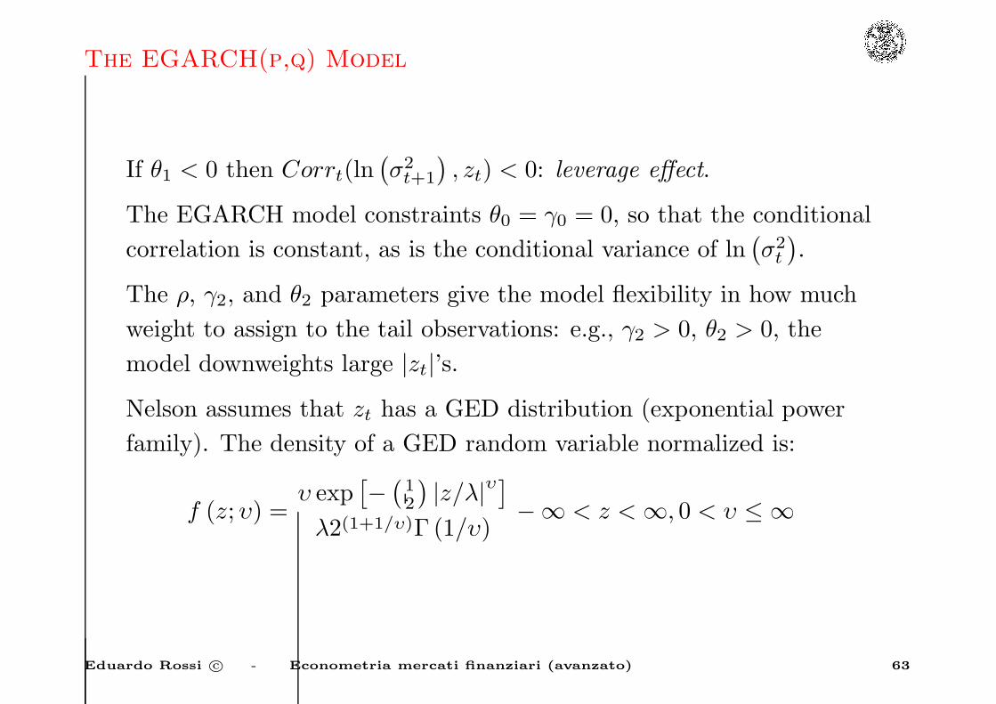
If θ1 < 0 then Corrt(ln(
σ2t+1
)
, zt) < 0: leverage effect.
The EGARCH model constraints θ0 = γ0 = 0, so that the conditional
correlation is constant, as is the conditional variance of ln(
σ2t
)
.
The ρ, γ2, and θ2 parameters give the model flexibility in how much
weight to assign to the tail observations: e.g., γ2 > 0, θ2 > 0, the
model downweights large |zt|’s.
Nelson assumes that zt has a GED distribution (exponential power
family). The density of a GED random variable normalized is:
f (z; υ) =υ exp
[
−(
12
)
|z/λ|υ]
λ2(1+1/υ)Γ (1/υ)−∞ < z <∞, 0 < υ ≤ ∞
Eduardo Rossi c© - Econometria mercati finanziari (avanzato) 63
The EGARCH(p,q) Model
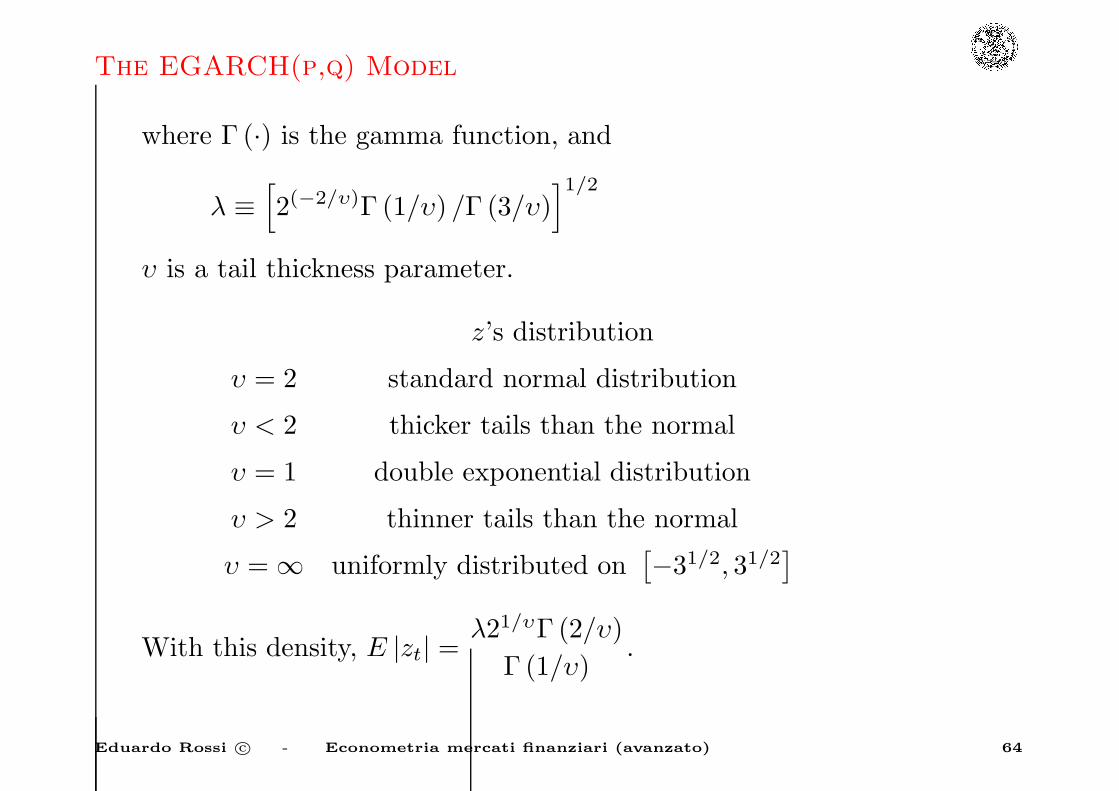
where Γ (·) is the gamma function, and
λ ≡[
2(−2/υ)Γ (1/υ) /Γ (3/υ)]1/2
υ is a tail thickness parameter.
z’s distribution
υ = 2 standard normal distribution
υ < 2 thicker tails than the normal
υ = 1 double exponential distribution
υ > 2 thinner tails than the normal
υ = ∞ uniformly distributed on[
−31/2, 31/2]
With this density, E |zt| =λ21/υΓ (2/υ)
Γ (1/υ).
Eduardo Rossi c© - Econometria mercati finanziari (avanzato) 64

The EGARCH(p,q) Model
The Generalized t Distribution takes the form:
f(
εtσ−1t ; η, ζ
)
=η
2σtbζ1/ηB (1/η, ζ) [1 + |εt|η / (ζbηση
t )]ζ+1/η
where B (1/η, ζ) ≡ Γ (1/η) Γ (ζ) Γ (1/η + ζ) denotes the beta function,
b ≡ [Γ (ζ) Γ (1/η) /Γ (3/η) Γ (ζ − 2/η)]1/2
and ζη > 2, η > 0 and ζ > 0. The factor b makes V ar(
εtσ−1t
)
= 1.
The Generalized t nests both the Student’s t distribution and the
GED.
Eduardo Rossi c© - Econometria mercati finanziari (avanzato) 65

The EGARCH(p,q) Model
The Student’s t-distribution sets η = 2 and ζ = 12 times the degree of
freedom
The GED is obtained for ζ = ∞. The GED has only one shape
parameter η, which is apparently insufficient to fit both the central
part and the tails of the conditional distribution.
Eduardo Rossi c© - Econometria mercati finanziari (avanzato) 66

Stationarity of EGARCH(p,q)
In order to simply state the stationarity conditions, we write the
EGARCH(p,q) model as:
[
1 −
p∑
i=1
βiLi
]
ln(
σ2t
)
= ω +
q∑
i=1
αiLi [φzt + ψ (|zt| −E |zt|)]
ln(
σ2t
)
=
[
1 −
p∑
i=1
βi
]
−1
ω +
[
1 −
p∑
i=1
βiLi
]
−1 [ q∑
i=1
αiLi
]
g (zt)
ln(
σ2t
)
= ω∗ +
∞∑
i=1
ϕig (zt−i)
Eduardo Rossi c© - Econometria mercati finanziari (avanzato) 67

Stationarity of EGARCH(p,q)
Given φ 6= 0 or ψ 6= 0, then
∣
∣ln(
σ2t
)
− ω∗∣
∣ <∞ a.s. when∞∑
i=1
ϕ2i <∞
follows from the independence and finite variance of the g (zt) and
from Billingsley (1986, Theorem 22.6). From this we have that∣
∣
∣
∣
ln
(
σ2t
exp(ω∗)
)∣
∣
∣
∣
< ∞ a.s.
∣
∣
∣
∣
σ2t
exp(ω∗)
∣
∣
∣
∣
< ∞ a.s.
{
exp (−ω∗)σ2t
}
<∞, {exp (−ω∗/2) εt} <∞, a.s., where εt = ztσt, zt
is i.i.d.. We can also show that they are ergodic and strictly
stationarity.
Eduardo Rossi c© - Econometria mercati finanziari (avanzato) 68

Stationarity of EGARCH(p,q)
The first two moments of ln(
σ2t
)
− ω∗ are finite and time invariant :
E[
ln(
σ2t
)
− ω∗]
= 0 for all t
V ar[
ln(
σ2t
)
− ω∗]
= V ar (g (zt))∞∑
i=1
ϕ2i
since V ar (g (zt)) is finite and the distribution of(
ln(
σ2t
)
− ω∗)
is
independent of t, the first two moments of(
ln(
σ2t
)
− ω∗)
are finite
and time invariant, so(
ln(
σ2t
)
− ω∗)
is covariance stationary if∞∑
i=1
ϕ2i <∞. If
∞∑
i=1
ϕ2i = ∞, then
∣
∣ln(
σ2t
)
− ω∗∣
∣ = ∞ almost surely.
Eduardo Rossi c© - Econometria mercati finanziari (avanzato) 69
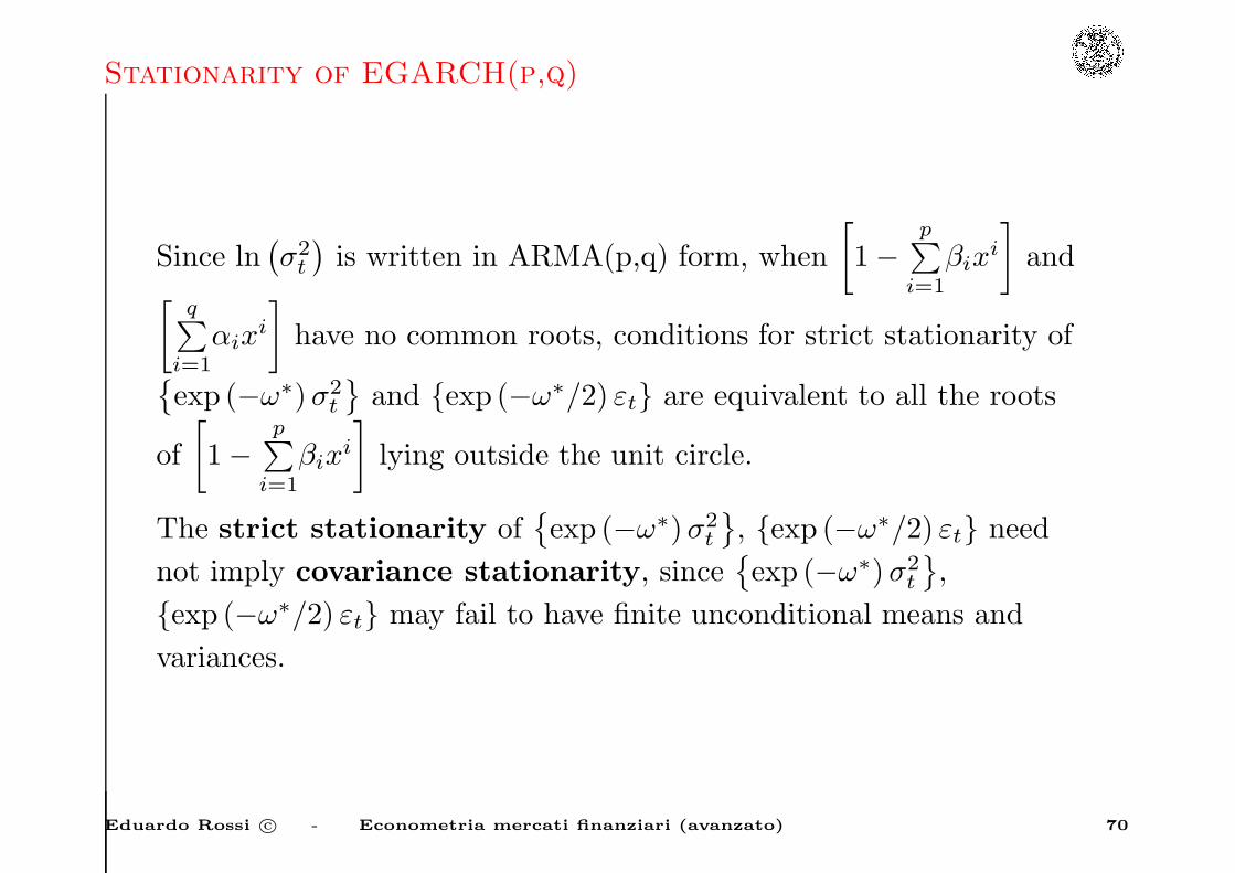
Stationarity of EGARCH(p,q)
Since ln(
σ2t
)
is written in ARMA(p,q) form, when
[
1 −p∑
i=1
βixi
]
and[
q∑
i=1
αixi
]
have no common roots, conditions for strict stationarity of{
exp (−ω∗)σ2t
}
and {exp (−ω∗/2) εt} are equivalent to all the roots
of
[
1 −p∑
i=1
βixi
]
lying outside the unit circle.
The strict stationarity of{
exp (−ω∗)σ2t
}
, {exp (−ω∗/2) εt} need
not imply covariance stationarity, since{
exp (−ω∗)σ2t
}
,
{exp (−ω∗/2) εt} may fail to have finite unconditional means and
variances.
Eduardo Rossi c© - Econometria mercati finanziari (avanzato) 70

Stationarity of EGARCH(p,q)
For some distribution of {zt} (e.g., the Student t with finite degrees
of freedom),{
exp (−ω∗)σ2t
}
and {exp (−ω∗/2) εt} typically have no
finite unconditional moments.
If the distribution of zt is GED and is thinner-tailed than the double
exponential (ν > 1), and if∞∑
i=1
ϕ2i <∞, then
{
exp (−ω∗)σ2t
}
and
{exp (−ω∗/2) εt} are not only strictly stationary and ergodic,
but have arbitrary finite moments, which in turn implies
that they are covariance stationary.
Eduardo Rossi c© - Econometria mercati finanziari (avanzato) 71

Other Asymmetric Models
The Non linear ARCH(p,q) model (Engle - Bollerslev 1986):
σγt = ω +
q∑
i=1
αi |εt−i|γ
+
p∑
i=1
βiσγt−i
σγt = ω +
q∑
i=1
αi |εt−i − k|γ
+
p∑
i=1
βiσγt−i
for k 6= 0, the innovations in σγt will depend on the size as well as the
sign of lagged residuals, thereby allowing for the leverage effect in
stock return volatility.
Eduardo Rossi c© - Econometria mercati finanziari (avanzato) 72
Other Asymmetric Models
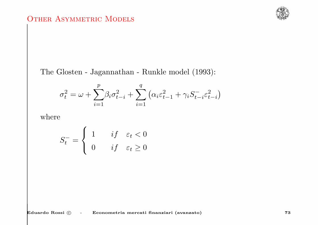
The Glosten - Jagannathan - Runkle model (1993):
σ2t = ω +
p∑
i=1
βiσ2t−i +
q∑
i=1
(
αiε2t−1 + γiS
−
t−iε2t−i
)
where
S−
t =
1 if εt < 0
0 if εt ≥ 0
Eduardo Rossi c© - Econometria mercati finanziari (avanzato) 73
Other Asymmetric Models
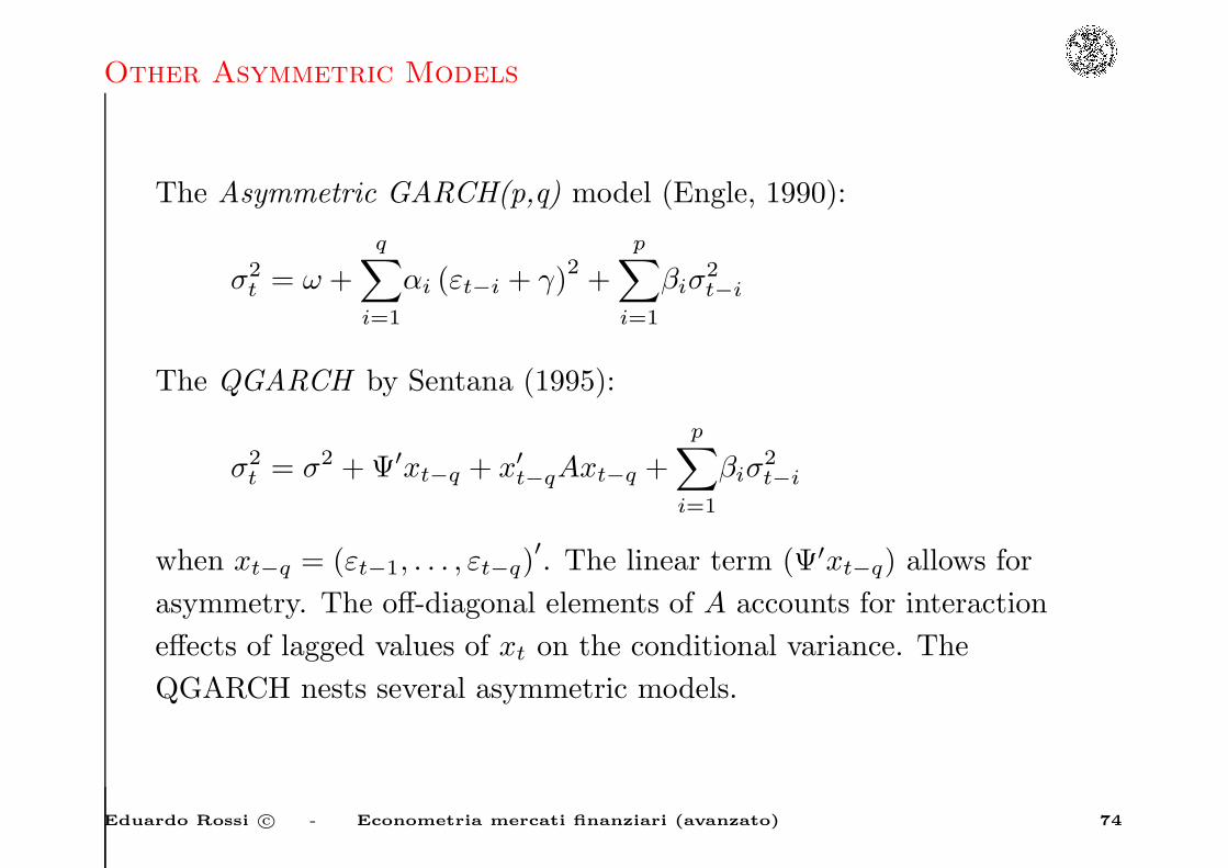
The Asymmetric GARCH(p,q) model (Engle, 1990):
σ2t = ω +
q∑
i=1
αi (εt−i + γ)2
+
p∑
i=1
βiσ2t−i
The QGARCH by Sentana (1995):
σ2t = σ2 + Ψ′xt−q + x′t−qAxt−q +
p∑
i=1
βiσ2t−i
when xt−q = (εt−1, . . . , εt−q)′
. The linear term (Ψ′xt−q) allows for
asymmetry. The off-diagonal elements of A accounts for interaction
effects of lagged values of xt on the conditional variance. The
QGARCH nests several asymmetric models.
Eduardo Rossi c© - Econometria mercati finanziari (avanzato) 74
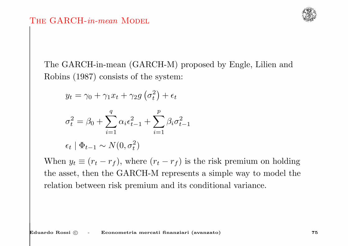
The GARCH-in-mean Model
The GARCH-in-mean (GARCH-M) proposed by Engle, Lilien and
Robins (1987) consists of the system:
yt = γ0 + γ1xt + γ2g(
σ2t
)
+ ǫt
σ2t = β0 +
q∑
i=1
αiǫ2t−1 +
p∑
i=1
βiσ2t−1
ǫt | Φt−1 ∼ N(0, σ2t )
When yt ≡ (rt − rf ), where (rt − rf ) is the risk premium on holding
the asset, then the GARCH-M represents a simple way to model the
relation between risk premium and its conditional variance.
Eduardo Rossi c© - Econometria mercati finanziari (avanzato) 75
The GARCH-in-mean Model
This model characterizes the evolution of the mean and the variance
of a time series simultaneously.
The GARCH-M model therefore allows to analize the possibility of
time-varying risk premium.
It turns out that:
yt | Φt−1 ∼ N(γ0 + γ1xt + γ2g(
σ2t
)
, σ2t )
In applications, g(
σ2t
)
=√
σ2t , g
(
σ2t
)
= ln(
σ2t
)
and g(
σ2t
)
= σ2t have
been used.
Eduardo Rossi c© - Econometria mercati finanziari (avanzato) 76

The News Impact Curve
• The news have asymmetric effects on volatility.
• In the asymmetric volatility models good news and bad news
have different predictability for future volatility.
• The news impact curve characterizes the impact of past return
shocks on the return volatility which is implicit in a volatility
model.
Eduardo Rossi c© - Econometria mercati finanziari (avanzato) 77

The News Impact Curve
Holding constant the information dated t− 2 and earlier, we can
examine the implied relation between εt−1 and σ2t , with σ2
t−i = σ2
i = 1, . . . , p.
This impact curve relates past return shocks (news) to current
volatility.
This curve measures how new information is incorporated into
volatility estimates.
Eduardo Rossi c© - Econometria mercati finanziari (avanzato) 78
The News Impact Curve
For the GARCH model the News Impact Curve (NIC) is centered on
ǫt−1 = 0.
GARCH(1,1):
σ2t = ω + αǫ2t−1 + βσ2
t−1
The news impact curve has the following expression:
σ2t = A+ αǫ2t−1
A ≡ ω + βσ2
Eduardo Rossi c© - Econometria mercati finanziari (avanzato) 79
The News Impact Curve
In the case of EGARCH model the curve has its minimum at
ǫt−1 = 0 and is exponentially increasing in both directions but with
different paramters.
EGARCH(1,1):
σ2t = ω + β ln
(
σ2t−1
)
+ φzt−1 + ψ (|zt−1| −E |zt−1|)
where zt = ǫt/σt. The news impact curve is
σ2t =
A exp
[
φ+ ψ
σǫt−1
]
for ǫt−1 > 0
A exp
[
φ− ψ
σǫt−1
]
for ǫt−1 < 0
A ≡ σ2β exp[
ω − α√
2/π]
φ < 0 ψ + φ > 0
Eduardo Rossi c© - Econometria mercati finanziari (avanzato) 80
The News Impact Curve
• The EGARCH allows good news and bad news to have different
impact on volatility, while the standard GARCH does not.
• The EGARCH model allows big news to have a greater impact
on volatility than GARCH model. EGARCH would have higher
variances in both directions because the exponential curve
eventually dominates the quadrature.
Eduardo Rossi c© - Econometria mercati finanziari (avanzato) 81
The News Impact Curve
The Asymmetric GARCH(1,1) (Engle, 1990)
σ2t = ω + α (ǫt−1 + γ)2 + βσ2
t−1
the NIC is
σ2t = A+ α (ǫt−1 + γ)
2
A ≡ ω + βσ2
ω > 0, 0 ≤ β < 1, σ > 0, 0 ≤ α < 1.
is asymmetric and centered at ǫt−1 = −γ.
Eduardo Rossi c© - Econometria mercati finanziari (avanzato) 82

The News Impact Curve
The Glosten-Jagannathan-Runkle model
σ2t = ω + αǫ2t + βσ2
t−1 + γS−
t−1ǫ2t−1
S−
t−1 =
1 if ǫt−1 < 0
0 otherwise
The NIC is
σ2t =
A+ αǫ2t−1 if ǫt−1 > 0
A+ (α+ γ) ǫ2t−1 if ǫt−1 < 0
A ≡ ω + βσ2
ω > 0, 0 ≤ β < 1, σ > 0, 0 ≤ α < 1, α+ β < 1
is centered at ǫt−1 = −γ.
Eduardo Rossi c© - Econometria mercati finanziari (avanzato) 83

The GARCH-in-mean Model
The GARCH-in-mean (GARCH-M) proposed by Engle, Lilien and
Robins (1987) consists of the system:
yt = γ0 + γ1xt + γ2g(
σ2t
)
+ ǫt
σ2t = β0 +
q∑
i=1
αiǫ2t−1 +
p∑
i=1
βiσ2t−1
ǫt | Φt−1 ∼ N(0, σ2t )
When yt ≡ (rt − rf ), where (rt − rf ) is the risk premium on holding
the asset, then the GARCH-M represents a simple way to model the
relation between risk premium and its conditional variance.
Eduardo Rossi c© - Econometria mercati finanziari (avanzato) 84

The GARCH-in-mean Model
This model characterizes the evolution of the mean and the variance
of a time series simultaneously.
The GARCH-M model therefore allows to analyze the possibility of
time-varying risk premium.
It turns out that:
yt | Φt−1 ∼ N(γ0 + γ1xt + γ2g(
σ2t
)
, σ2t )
In applications, g(
σ2t
)
=√
σ2t , g
(
σ2t
)
= ln(
σ2t
)
and g(
σ2t
)
= σ2t have
been used.
Eduardo Rossi c© - Econometria mercati finanziari (avanzato) 85

The News Impact Curve
• The news have asymmetric effects on volatility.
• In the asymmetric volatility models good news and bad news
have different predictability for future volatility.
• The news impact curve characterizes the impact of past return
shocks on the return volatility which is implicit in a volatility
model.
Eduardo Rossi c© - Econometria mercati finanziari (avanzato) 86
The News Impact Curve
Holding constant the information dated t− 2 and earlier, we can
examine the implied relation between εt−1 and σ2t , with σ2
t−i = σ2
i = 1, . . . , p.
This impact curve relates past return shocks (news) to current
volatility.
This curve measures how new information is incorporated into
volatility estimates.
Eduardo Rossi c© - Econometria mercati finanziari (avanzato) 87

The News Impact Curve
For the GARCH model the News Impact Curve (NIC) is centered on
ǫt−1 = 0.
GARCH(1,1):
σ2t = ω + αǫ2t−1 + βσ2
t−1
The news impact curve has the following expression:
σ2t = A+ αǫ2t−1
A ≡ ω + βσ2
Eduardo Rossi c© - Econometria mercati finanziari (avanzato) 88

The News Impact Curve
In the case of EGARCH model the curve has its minimum at
ǫt−1 = 0 and is exponentially increasing in both directions but with
different paramters.
EGARCH(1,1):
σ2t = ω + β ln
(
σ2t−1
)
+ φzt−1 + ψ (|zt−1| −E |zt−1|)
where zt = ǫt/σt. The news impact curve is
σ2t =
A exp
[
φ+ ψ
σǫt−1
]
for ǫt−1 > 0
A exp
[
φ− ψ
σǫt−1
]
for ǫt−1 < 0
A ≡ σ2β exp[
ω − α√
2/π]
φ < 0 ψ + φ > 0
Eduardo Rossi c© - Econometria mercati finanziari (avanzato) 89

The News Impact Curve
• The EGARCH allows good news and bad news to have different
impact on volatility, while the standard GARCH does not.
• The EGARCH model allows big news to have a greater impact
on volatility than GARCH model. EGARCH would have higher
variances in both directions because the exponential curve
eventually dominates the quadrature.
Eduardo Rossi c© - Econometria mercati finanziari (avanzato) 90

The News Impact Curve
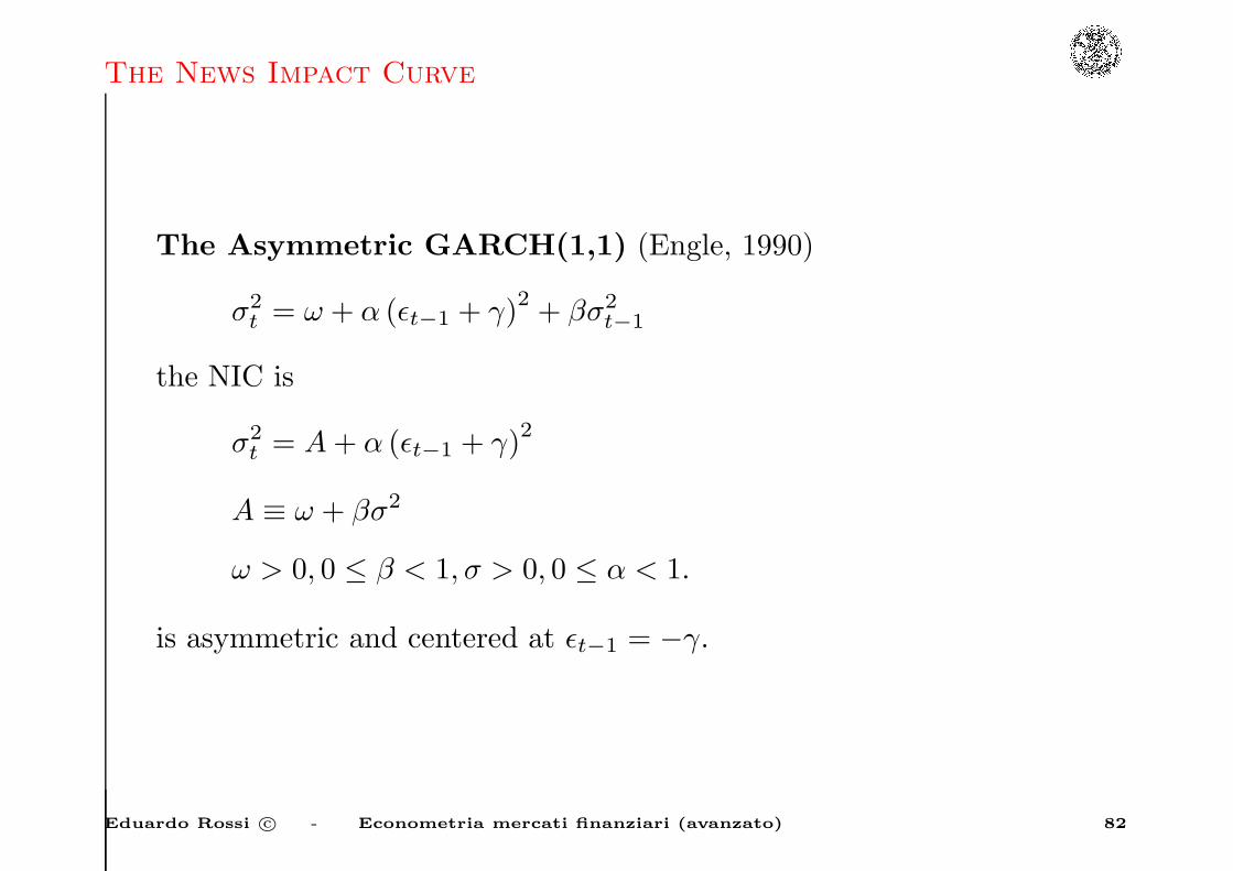
The Asymmetric GARCH(1,1) (Engle, 1990)
σ2t = ω + α (ǫt−1 + γ)2 + βσ2
t−1
the NIC is
σ2t = A+ α (ǫt−1 + γ)
2
A ≡ ω + βσ2
ω > 0, 0 ≤ β < 1, σ > 0, 0 ≤ α < 1.
is asymmetric and centered at ǫt−1 = −γ.
Eduardo Rossi c© - Econometria mercati finanziari (avanzato) 91
The News Impact Curve
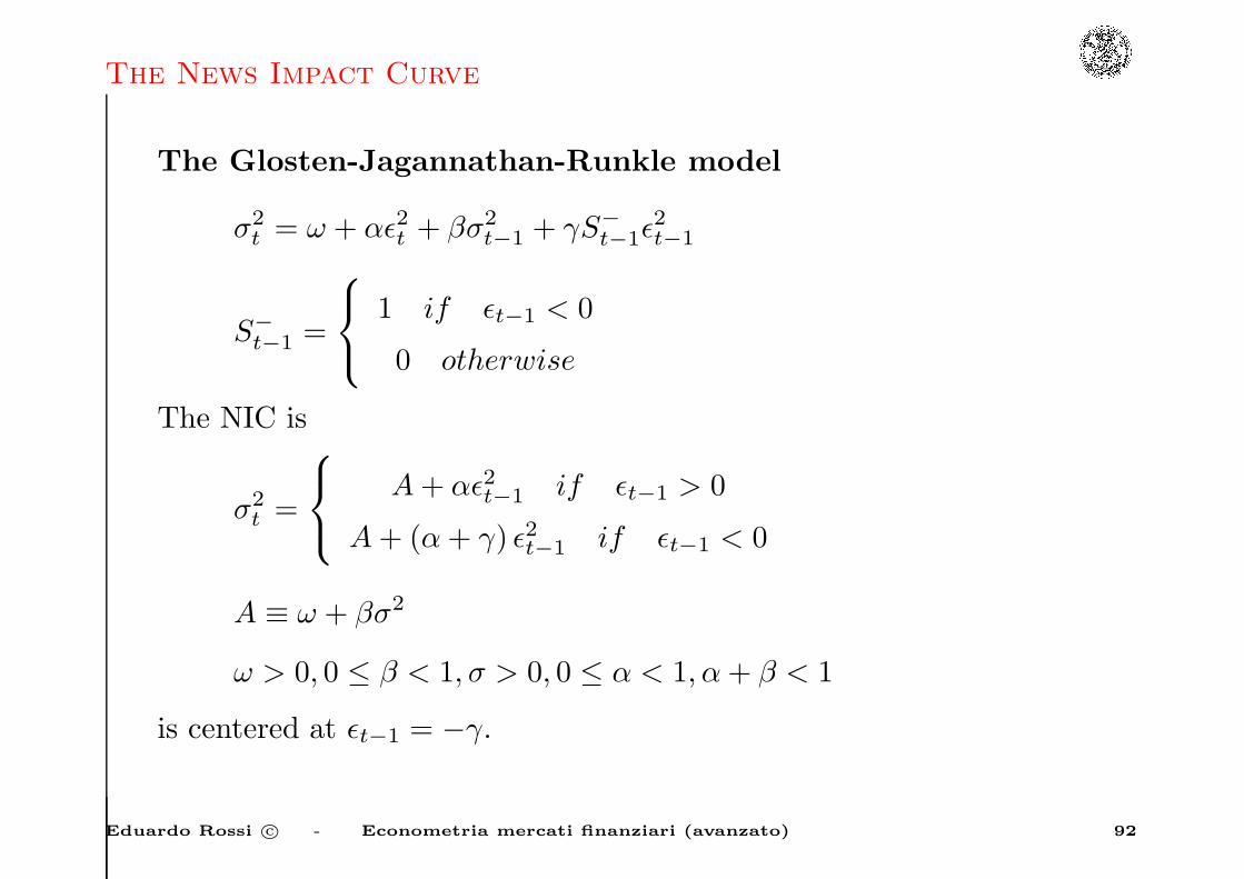
The Glosten-Jagannathan-Runkle model
σ2t = ω + αǫ2t + βσ2
t−1 + γS−
t−1ǫ2t−1
S−
t−1 =
1 if ǫt−1 < 0
0 otherwise
The NIC is
σ2t =
A+ αǫ2t−1 if ǫt−1 > 0
A+ (α+ γ) ǫ2t−1 if ǫt−1 < 0
A ≡ ω + βσ2
ω > 0, 0 ≤ β < 1, σ > 0, 0 ≤ α < 1, α+ β < 1
is centered at ǫt−1 = −γ.
Eduardo Rossi c© - Econometria mercati finanziari (avanzato) 92