EXOGENOUS GROWTH MODELS -...
96
EXOGENOUS GROWTH MODELS Lorenza Rossi Goethe University 2011-2012
-
Upload
phamnguyet -
Category
Documents
-
view
219 -
download
4
Transcript of EXOGENOUS GROWTH MODELS -...
EXOGENOUS GROWTH MODELS
Lorenza Rossi
Goethe University 2011-2012

Course Outline
FIRST PART - GROWTH THEORIES
Exogenous GrowthThe Solow ModelThe Ramsey model and the Golden Rule
Introduction to Endogenous Growth modelsThe AK model - Romer (1990)Two sector model of Endogenous growth
SECOND PART - BUSINESS CYCLE
Introduction to NK modelThe BMW model as a static approximation of a forward-looking NKmodelThe BMW model in a closed economy: ination targeting versus TaylorrulesThe BMW model in an open economy: comparisons with the MundelFleming model

TODAY
Brief Review Growth Stylized Facts
Introduction to the Solow Model
DerivationsThe model performance and stylized facts

STYLIZED FACT 1
There is an enormous variation in the per capita income acrosseconomies. The poorest countries have per capita income that areless than 5 percent of per capita incomes in the riches countries.
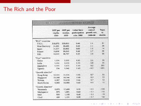
The Rich and the Poor

The Rich and the Poor
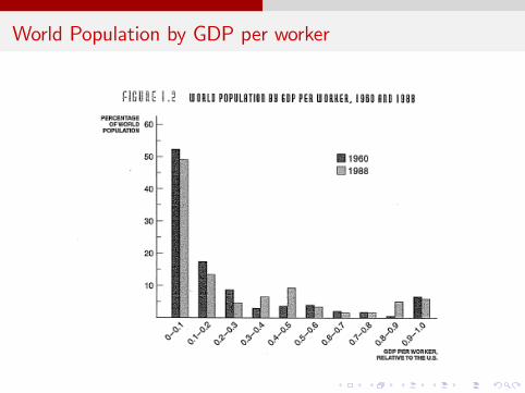
World Population by GDP per worker
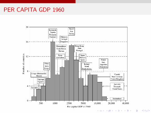
PER CAPITA GDP 1960

PER CAPITA GDP 2000
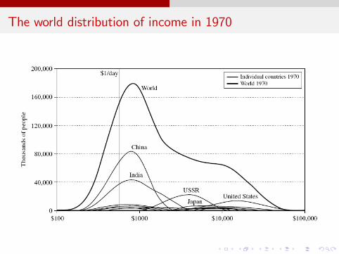
The world distribution of income in 1970

The world distribution of income in 2000

STYLIZED FACT 2
Rates of Economic Growth vary substantially across countries
STYLIZED FACT 3
Growth rates are not generally constant over time. For the world aswhole, growth rates were close to zero over most of the history buthave increased sharply in the twentieth century. For individualcountries, growth rates also change over time.

STYLIZED FACT 4
A country relative position in the world distribution of per capitaincomes is not immutable. Countries can move from being poor tobeing rich, or viceversa.
EXAMPLE: Venezuela vs Italy.

Fifteen Growth Miracles
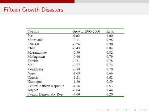
Fifteen Growth Disasters
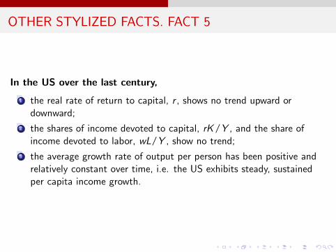
OTHER STYLIZED FACTS. FACT 5
In the US over the last century,
1 the real rate of return to capital, r , shows no trend upward ordownward;
2 the shares of income devoted to capital, rK/Y , and the share ofincome devoted to labor, wL/Y , show no trend;
3 the average growth rate of output per person has been positive andrelatively constant over time, i.e. the US exhibits steady, sustainedper capita income growth.

Real Per Capita GDP in the US

OTHER STYLIZED FACTS: FACT 6
Growth in output and growth in the volume of international tradeare closely related
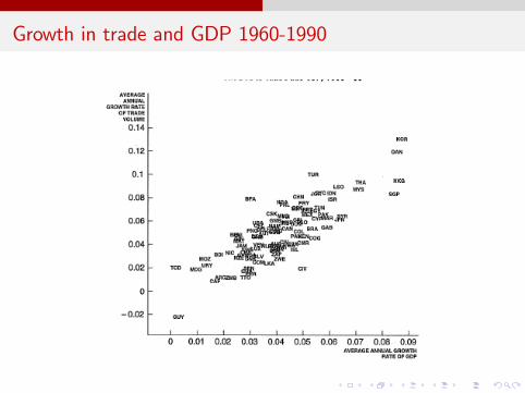
Growth in trade and GDP 1960-1990

OTHER STYLIZED FACTS: FACT 7
Both skilled and unskilled workers tend to migrate from poor to richcountries or regions
ROBERT LUCAS: this movements of labor tell us something about realwages. The returns of both skilled and unskilled
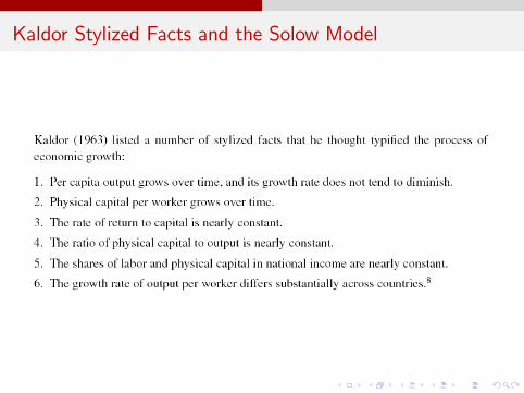
Kaldor Stylized Facts and the Solow Model
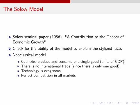
The Solow Model
Solow seminal paper (1956). "A Contribution to the Theory ofEconomic Growth"
Check for the ability of the model to explain the stylized facts
Neoclassical model
Countries produce and consume one single good (units of GDP);There is no international trade (since there is only one good)Technology is exogenousPerfect competition in all markets
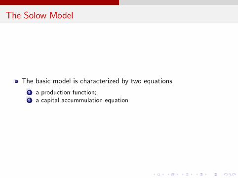
The Solow Model
The basic model is characterized by two equations1 a production function;2 a capital accummulation equation
The Solow Model
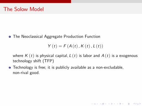
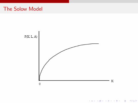
The Neoclassical Aggregate Production Function
Y (t) = F (A (t) ,K (t) , L (t))
where K (t) is physical capital, L (t) is labor and A (t) is a exogenoustechnology shift (TFP)
Technology is free; it is publicly available as a non-excludable,non-rival good.

The Solow Model: Key Assumption
Assumptions
F exhibits constant return to scale in K and L =) F is linearhomogeneous (homegeneous of degree 1)
The Solow Model: Key Assumption
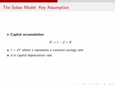
Capital accumulation
K = I d K .
I = sY where s represents a constant savings rate.
d is capital depreciation rate

The Solow Model
The Inada Conditions
limK!0
FK () = ∞ and limK!∞
FK () = 0 for all L > 0 and all A
limL!0
FL () = ∞ and limL!∞
FL () = 0 for all K > 0 and all A
Important in ensuring the existence of interior equilibria.
The Solow Model
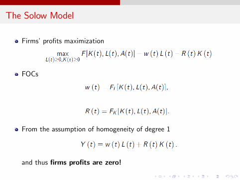
Firmsprots maximization
FOCs
From the assumption of homogeneity of degree 1
and thus rms prots are zero!
The Solow Model
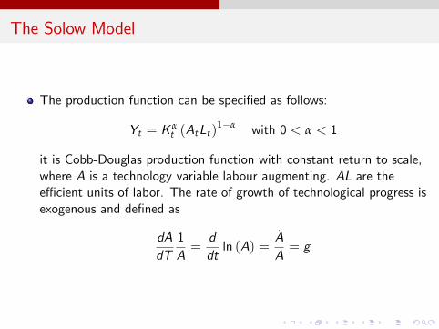
The production function can be specied as follows:
Yt = K αt (AtLt )
1α with 0 < α < 1
it is Cobb-Douglas production function with constant return to scale,where A is a technology variable labour augmenting. AL are thee¢ cient units of labor. The rate of growth of technological progress isexogenous and dened as
dAdT
1A=ddtln (A) =
AA= g
The Solow Model
The Solow Model
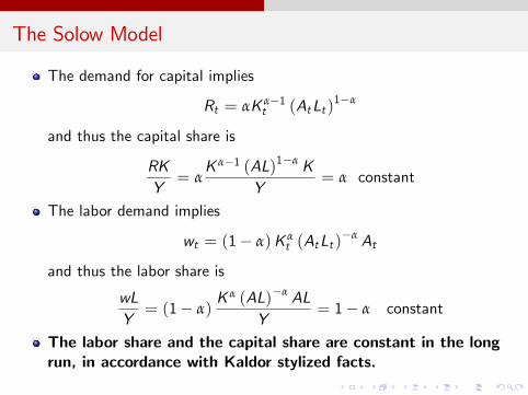
The demand for capital implies
Rt = αK α1t (AtLt )
1α
and thus the capital share is
RKY= α
K α1 (AL)1α KY
= α constant
The labor demand implies
wt = (1 α)K αt (AtLt )
α At
and thus the labor share is
wLY= (1 α)
K α (AL)α ALY
= 1 α constant
The labor share and the capital share are constant in the longrun, in accordance with Kaldor stylized facts.
The Solow Model
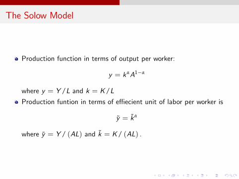
Production function in terms of output per worker:
y = kαA1α
where y = Y /L and k = K/LProduction funtion in terms of e¢ ecient unit of labor per worker is
y = kα
where y = Y / (AL) and k = K/ (AL) .
The Solow Model
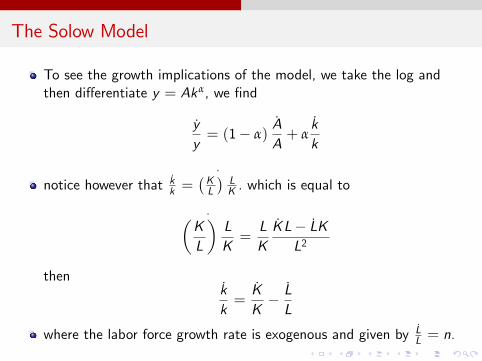
To see the growth implications of the model, we take the log andthen di¤erentiate y = Akα, we nd
yy= (1 α)
AA+ α
kk
notice however that kk =K
L
LK . which is equal to
KL
LK=LKKL LKL2
thenkk=KK LL
where the labor force growth rate is exogenous and given by LL = n.
The Solow Model
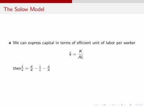
We can express capital in terms of e¢ cient unit of labor per worker
k =KAL
thenkk =
KK
LL
AA
The Solow Model
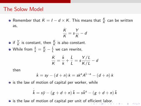
Remember that K = I d K . This means that KK can be writtenas,
KK= s
YK d
if YK is constant, then KK is also constant.
While from kk =
KK
LL we can rewrite,
KK=kk+LL= s
Y /LK/L
d
thenk = sy (d + n) k = skαA1α (d + n) k
is the law of motion of capital per worker, whilek = sy (g + d + n) k = skα (g + d + n) k
is the law of motion of capital per unit of e¢ cient labor.
The Solow Model
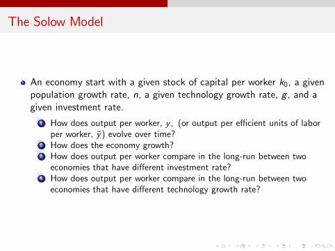
An economy start with a given stock of capital per worker k0, a givenpopulation growth rate, n, a given technology growth rate, g , and agiven investment rate.
1 How does output per worker, y , (or output per e¢ cient units of laborper worker, y) evolve over time?
2 How does the economy growth?3 How does output per worker compare in the long-run between twoeconomies that have di¤erent investment rate?
4 How does output per worker compare in the long-run between twoeconomies that have di¤erent technology growth rate?
The Solow Model
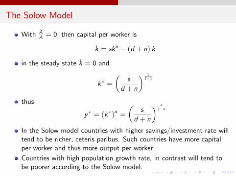
With AA = 0, then capital per worker is
k = skα (d + n) k
in the steady state k = 0 and
k =
sd + n
11α
thus
y = (k)α =
s
d + n
α1α
In the Solow model countries with higher savings/investment rate willtend to be richer, ceteris paribus. Such countries have more capitalper worker and thus more output per worker.Countries with high population growth rate, in contrast will tend tobe poorer according to the Solow model.
The Solow Model
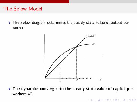
The Solow diagram determines the steady state value of output perworker
The dynamics converges to the steady state value of capital perworkers k.

The Solow Model
Balanced growth. Notice thatk = skα (d + n) k
kk
= 0 impliesKL= constant =) K
K= n
yy
= 0 impliesYL= constant =) Y
Y= n
cc
= 0 impliesCL= constant =) C
C= n
KY
= k1α =s
d + nin steady state
The Solow Model
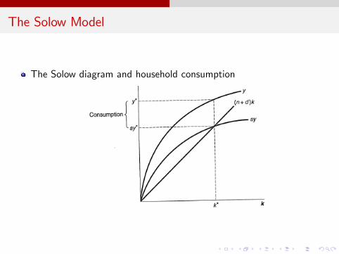
The Solow diagram and household consumption

The Solow Model. The Golden rule
Consumption isct = F (kt ) sF (kt )
At the steady state consumption is
c = F (k) sF (k) = (k)α (d + n) k
consumption is maximum if
∂c∂k= 0 : F 0 (k) (d + n) = 0
The Solow Model. The Golden rule
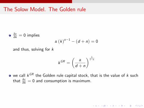
∂c∂k = 0 implies
α (k)α1 (d + n) = 0and thus, solving for k
kGR =
α
d + n
11α
we call kGR the Golden rule capital stock, that is the value of k suchthat ∂c
∂k = 0 and consumption is maximum.
The Solow Model. The Golden rule
The Solow Model. The Golden rule
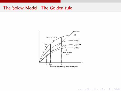
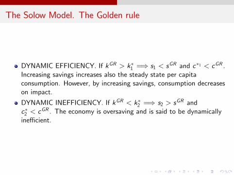
DYNAMIC EFFICIENCY. If kGR > k1 =) s1 < sGR and c1 < cGR .Increasing savings increases also the steady state per capitaconsumption. However, by increasing savings, consumption decreaseson impact.
DYNAMIC INEFFICIENCY. If kGR < k2 =) s2 > sGR andc2 < c
GR . The economy is oversaving and is said to be dynamicallyine¢ cient.

The Solow Model
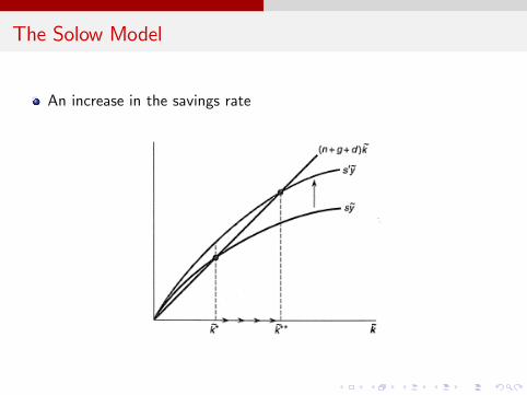
An increase in the investment rate s
the steady state value of capital per worker increases.

The Solow Model
An increase in population growth
The Solow Model
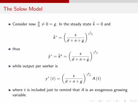
Consider now AA 6= 0 = g . In the steady state
k = 0 and
k =
sd + n+ g
11α
thus
y = kα =
s
d + n+ g
α1α
while output per worker is
y (t) =
sd + n+ g
α1α
A (t)
where t is included just to remind that A is an exogenous growingvariable.
The Solow Model
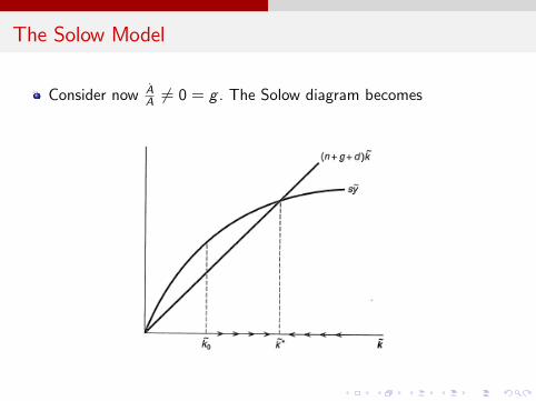
Consider now AA 6= 0 = g . The Solow diagram becomes

The Solow Model
Balanced growth. Notice thatk = skα (g + d + n) k
kk
= 0 impliesKK= g + n and
kk= g
yy
= 0 impliesYY= g + n and
yy= g
cc
= 0 impliesCC= g + n and
cc= g
nally notice that given KK =
YY =)
KK
YY = 0 and thus
KY=
sg + n+ d
= constant
The Solow Model
THE BALANCED GROWTH PATH. In the Solow model thegrowth process follows a balanced growth path if the GDP perworker, consumption per worker, the real wage per worker andcapital per worker, all grow at one and the same constant rate,g , the labor force, i.e. population grows at a constant rate n,GDP, consumption and capital grow at a common rate, g + n,the capital-output ratio is constant and the rate of return oncapital is constant.
The Solow Model
An increase in the savings rate
The Solow Model
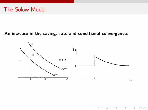
An increase in the savings rate and conditional convergence.
The Solow Model
Output per worker along the balanced growth path isdetermined by technology, investment rate and the populationgrowth rateChanges in the investment rate and the population growth ratea¤ect the long-run level of output per worker, but do not a¤ectits long-run growth rate.Policy changes do not have long-run growth e¤ects.Policy changes can have level e¤ects, that is a permanentpolicy change can permanently raise (or lower) the level of percapita output.Conditional convergence.
The Ramsey Growth Model
The Solow model:
The rst general equilibrium model with production side.
It is empirically testable.
Lacks microfoundations (saving is not determined exogenously)
Exogenous technological progress explains all.
The Ramsey Model
Introduces endogenous savings/consumption decision
Optimal consumption
The decentralized equilibrium can be compared with the Paretoe¢ cient equilibrium
The Ramsey Growth Model
The decentralized model
Two agents
Households. maximize their life-time utility subject to an intertemporalbudget constraintFirms: maximize prots subject to their factor accumulation constraint
General Equilibrium. Demand=Supply.
The Social Planner model
The social planner maximizes the householdsutility subject toaggregate resource constraint of the economy.
If the decentralized solution coincide with the Social Planner solution,then the outcome is Pareto optimal.
The Ramsey Growth Model
The Household Problem
One innitely-lived household maximizing the intertemporal utilityZ ∞
0u (ct ) Lteρtdt =
Z ∞
0u (ct ) Lte(nρ)tdt
where ρ is the discount factor. A higher ρ implies a smallerdesiderability of future consumption in terms of utility compared toutility obtained by current consumption.
where u0 (c) > 0 and u00 (c) < 0 and limc!0 u0 (c) = ∞ andlimc!∞ u0 (c) = 0 (Inada Conditions)
Population growth rate is constant (equal to n) and at time t = 0there is only one individual in the economy (i.e. L0 = 1), so that thetotal population at any time t is given by Lt = ent and thus LL = n.
The Ramsey Growth Model
The Household Problem
The household budget constraint is
B = wtLt + rtBt Ct
where B are assets, w is the wage rate, r is the interest rate. In percapita terms
b = wt + (rt n) bt ct
The Ramsey Growth Model
The Household Problem
The trasversality condition
limt!∞
0BBBBB@btetZ0
(rsn)ds
1CCCCCA 0
the present value of current and future assets must be asymptoticallynonnegative
households cannot borrow innitely until the end of their economiclife cycle
the householdsdebt cannot increase at a rate asymptotically higherthan the interest rate

The Ramsey Growth Model
The Household Problem
Writing the Hamiltonian
H =Z ∞
0u (ct ) e(nρ)tdt + µt (wt + (rt n) bt ct )
FOCs with respect to ct (control variable) and bt (state variable).
∂H∂c
= 0 : u0 (ct ) e(nρ)t = µt
∂H∂b
= µ : (rt n) µt = µ
∂H∂µ
= b : wt + (rt n) µt ct = b (is the constraint)

The Ramsey Growth Model
The Household Problem
From the rst FOC
u0 (ct ) e(nρ)t = µt =) µt = u00(ct ) e(nρ)t c+(n ρ) u0 (ct ) e(nρ)t
combining with the second FOC, i.e. with (rt n) µt = µ, we get
(rt n) µt = u00(ct ) e(nρ)t c + (n ρ) u0 (ct ) e(nρ)t
or
(rt n) u0 (ct ) e(nρ)t = u00(ct ) e(nρ)t c + (n ρ) u0 (ct ) e(nρ)t
simplifying and rearranging we nd the Euler equation
rt = ρ u00(c) cu0 (c)
!cc
The Ramsey Growth Model
The Household Problem
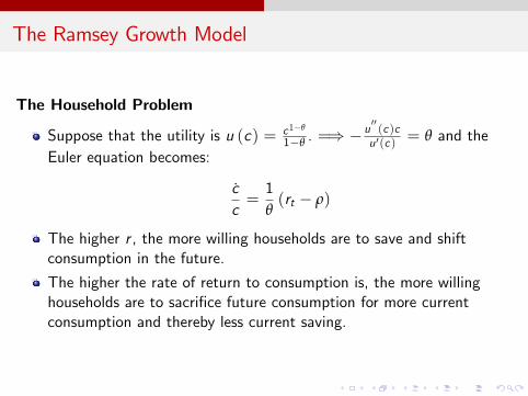
Suppose that the utility is u (c) = c1θ
1θ . =) u00(c )c
u 0(c ) = θ and theEuler equation becomes:
cc=1θ(rt ρ)
The higher r , the more willing households are to save and shiftconsumption in the future.
The higher the rate of return to consumption is, the more willinghouseholds are to sacrice future consumption for more currentconsumption and thereby less current saving.

The Ramsey Growth Model
Firms Problem
Prots Maximization
π = F (K , L) (r + δ)K wL
with F (K , L) Cobb-Douglas with constant return to scale
Focs of the static problem
f 0 (k) = (r + d)
f (k) kf 0 (k) = w

The Ramsey Growth Model
Equilibrium
The law of motion of per capita capital
k = f (k) (n+ d) k c
The law of motion of per capita consumption
cc=1θ
f 0 (k) d ρ
it is a 2x2 system of di¤erential equation which denes theequilibrium.

The Ramsey Growth Model
The Steady State
k = 0 : f (k) c = (n+ d) k
The law of motion of per capita consumption
cc= 0 : f 0 (k) = d + ρ

The Ramsey Growth Model
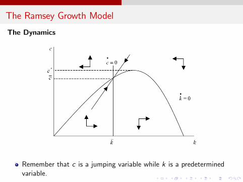
The Dynamics
Notice that ∂k∂c = 1 < 0, while
∂c∂k =
1θ f
00(k) c < 0
The Ramsey Growth Model
The Dynamics
Remember that c is a jumping variable while k is a predeterminedvariable.
The Ramsey Growth Model
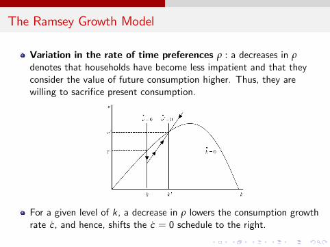
Variation in the rate of time preferences ρ : a decreases in ρdenotes that households have become less impatient and that theyconsider the value of future consumption higher. Thus, they arewilling to sacrice present consumption.
For a given level of k, a decrease in ρ lowers the consumption growthrate c , and hence, shifts the c = 0 schedule to the right.

The Ramsey Growth Model
To maintain consumption constant the capital stock must increase sothat, in the new long-run equilibrium, consumption, capital andoutput per capita attain a higher level (k 0 > k, c 0 > c).Consumption jumps along the saddle path, whereas k at the samelevel k. The reduction in consumption boosts saving and therebyleads to a increase in capital stock, until it reaches k 0 . =) incomeper capita level rises, with positive consumption growth rate untilreaching the higher levels of consumption and capital (c 0, k 0), andincome.
The Ramsey Growth Model
The Modiced Golden Rule
In the Solow model the Golden rule implies
f 0 (k) = n+ d
In the Ramsey model, the modied gold rule, which is obtained fromconsumer problem implies
f 0kRamsey
= ρ+ d
Given that the transersality condition implies that ρ > n.
+
In the Ramsey model, the long-run equilibrium level of capital perworker is lower that in the Solow model. In the Ramsey modelhouseholds save less since there is discounting of future utility.
The Ramsey Growth Model
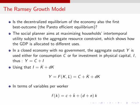
Is the decentralized equilibrium of the economy also the rstbest-outcome (the Pareto e¢ cient equilibrium)?
The social planner aims at maximizing householdsintertemporalutility subject to the aggregate resource constraint, which shows howthe GDP is allocated to di¤erent uses.
In a closed economy with no government, the aggregate output Y isused either for consumption C or for investment in physical capital, I ,thus : Y = C + I
Using that I = K + dK
Y = F (K , L) = C + K + dK
In terms of variables per worker
f (k) = c + k + (d + n) k
The Ramsey Growth Model
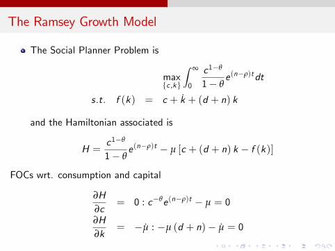
The Social Planner Problem is
maxfc ,kg
Z ∞
0
c1θ
1 θe(nρ)tdt
s.t. f (k) = c + k + (d + n) k
and the Hamiltonian associated is
H =c1θ
1 θe(nρ)t µ [c + (d + n) k f (k)]
FOCs wrt. consumption and capital
∂H∂c
= 0 : cθe(nρ)t µ = 0
∂H∂k
= µ : µ (d + n) µ = 0
The Ramsey Growth Model
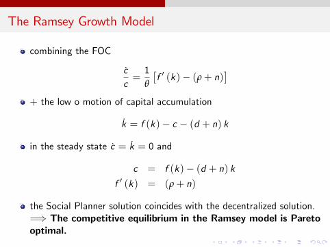
combining the FOC
cc=1θ
f 0 (k) (ρ+ n)
+ the low o motion of capital accumulation
k = f (k) c (d + n) k
in the steady state c = k = 0 and
c = f (k) (d + n) kf 0 (k) = (ρ+ n)
the Social Planner solution coincides with the decentralized solution.=) The competitive equilibrium in the Ramsey model is Paretooptimal.
The Solow Model with Human Capital
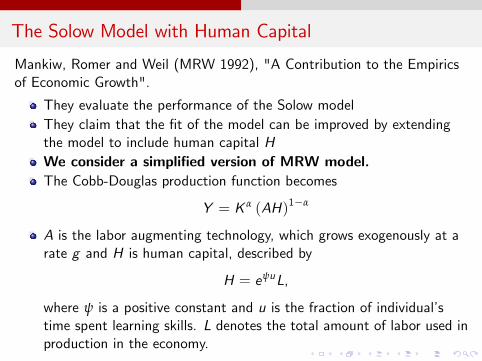
Mankiw, Romer and Weil (MRW 1992), "A Contribution to the Empiricsof Economic Growth".
They evaluate the performance of the Solow modelThey claim that the t of the model can be improved by extendingthe model to include human capital HWe consider a simplied version of MRW model.The Cobb-Douglas production function becomes
Y = K α (AH)1α
A is the labor augmenting technology, which grows exogenously at arate g and H is human capital, described by
H = eψuL,
where ψ is a positive constant and u is the fraction of individualstime spent learning skills. L denotes the total amount of labor used inproduction in the economy.

The Solow Model with Human Capital
Notice that if u = 0 then H = L,that is all labor is unskilled.
By taking the rst the log and then the derivative of H with respectto u
log (H) = ψu + log (L)
thend log (H)du
= ψ =) dHdu
= ψH
example u = 1 (one additional year of schooling), with ψ = 0.1 thenH increases by 10%.
This forumlation is intended to match the empirical literature onlabor economics that nds that an additional year of schoolingincreases the productivity of the worker and than its wage by 10%.
The Solow Model with Human Capital
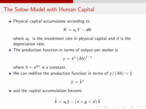
Physical capital accumulates according to
K = skY dK
where sK is the investment rate in physical capital and d is thedepreciation rate.The production function in terms of output per worker is
y = kα (Ah)1α
where h = eψu is a constant.We can redine the production function in terms of y/(Ah) = y
y = kα
and the capital accumulation becoms
k = sk y (n+ g + d) k
The Solow Model with Human Capital
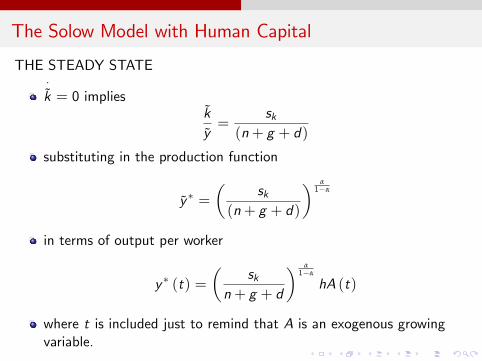
THE STEADY STATEk = 0 implies
ky=
sk(n+ g + d)
substituting in the production function
y =
sk(n+ g + d)
α1α
in terms of output per worker
y (t) =
skn+ g + d
α1α
hA (t)
where t is included just to remind that A is an exogenous growingvariable.

The Solow Model with Human Capital
From
y (t) =
skn+ g + d
α1α
hA (t)
we can state that some countries are rich because they:1 have higher investment in physical capital;2 spend a large fraction of time accumulating skills h = eψu ;3 have low population rate;4 have higher level of technology.
The Solow Model with Human Capital
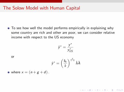
To see how well the model performs empirically in explaining whysome country are rich and other are poor, we can consider relativeincome with respect to the US economy
y =y
y US
or
y =skx
α1α
hA
where x = (n+ g + d) .

The Solow Model with Human Capital
The Fit of the Neoclassical Growth model, 1997 (source: Jones book)
The Solow Model with Human Capital
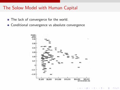
The lack of convergerce for the world.
Conditional convergence vs absolute convergence

The Green Solow Model and the Environmental KunetzCurve
Brock and Taylor (BT), 2010, Journal of Economic Growth
Environmental Kunetz Curve (EKC): is a humpshaped relationshipbetween environmental degradation and per capita income. At lowlevel of economic activity, the environment is worsening. As theeconomic activity increases environmental degradation peacks. Then,as a country becomes richer and richer, environmental degradationbegins to fall.
BT use a simple variant of the basic Solow model with DR in capitaland technologycal progress for abatement. They provide a theoreticalexplanation of the EKC and for abatement and emission intensity.They also derive an estimating equation for pollution convergence.

The Green Solow Model and the Environmental KunetzCurve
US evidence:1 Emissions per unit of output have been falling for a long period oftime

The Green Solow Model and the Environmental KunetzCurve
US evidence:2. Emission per unit of output were falling before absolute emissionsstarted to fall

The Green Solow Model and the Environmental KunetzCurve
US evidence:
3. Abatement cost per unit of output have been relatively constant

The Green Solow Model and the Environmental KunetzCurve
EU evidence:
European data show a strong evidence of an Environmental Kunetzcurve relationship
The evidence on cross-country data is mixed

The Green Solow Model
The Green Solow model augments the standard Solow model withpollution and abatement activityThe production function is
Y = F (K ,BL)
where B is the labor augmenting technology.the low of motion of capital is standard
K = sY dKNet Emission of Pollution E
E = ΩF ΩAF ,FA
= ΩF
1 A
1,FA
F
= ΩFa (θ)
where Ω is pollution from Y , A is the abatement with CRS productionfunction A
1, F
A
F
, and technology growth at exogenous rate gA. F
is total production activity, FA is total abatement activity. θ = F AF
and a (θ) = 1 A (1, θ) with a (0) = 1, a0 (θ) < 0, and a00 (θ) > 0.
The Green Solow Model
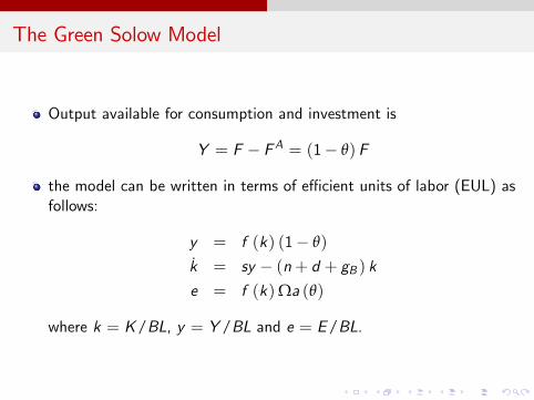
Output available for consumption and investment is
Y = F FA = (1 θ) F
the model can be written in terms of e¢ cient units of labor (EUL) asfollows:
y = f (k) (1 θ)
k = sy (n+ d + gB ) ke = f (k)Ωa (θ)
where k = K/BL, y = Y /BL and e = E/BL.
The Green Solow Model
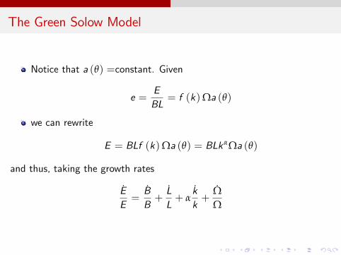
Notice that a (θ) =constant. Given
e =EBL
= f (k)Ωa (θ)
we can rewrite
E = BLf (k)Ωa (θ) = BLkαΩa (θ)
and thus, taking the growth rates
EE=BB+LL+ α
kk+
ΩΩ

The Green Solow Model
Easy to understand if we rewrite
EE= α
kk|z
transitionalcomponent
+ gB + n gA| z gE
Emission growthalong the BGP
The Green Solow Model
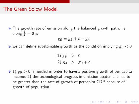
The growth rate of emission along the balanced growth path, i.e.along k
k = 0 isgE = gB + n gA
we can dene substainable growth as the condition implying gE < 0
1) gB > 0
2) gA > gB + n
1) gB > 0 is needed in order to have a positive growth of per capitaincome; 2) the technological progress in emission abatement has tobe greater than the rate of growth of percapita GDP because ofgrowth of population
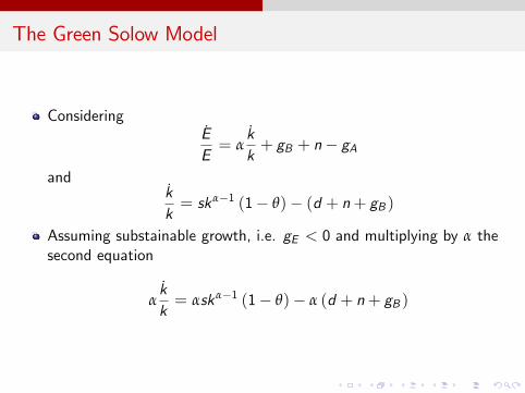
The Green Solow Model
ConsideringEE= α
kk+ gB + n gA
andkk= skα1 (1 θ) (d + n+ gB )
Assuming substainable growth, i.e. gE < 0 and multiplying by α thesecond equation
αkk= αskα1 (1 θ) α (d + n+ gB )

The Green Solow Model and the Environmental KunetzCurve

The Green Solow Model and the Environmental KunetzCurve
PROPOSITION 1
If growth is substainable gE < 0 and k (0) < k (T ) , then emissionsgrow initially and then fall continuously. An EKC occurs.If growth is substainable gE < 0 and k (0) > k (T ) , then emissionsfall continuouslyIf growth is unsubstainable gE > 0, then emissions growth but at adecreasing rate.
PROPOSITION 2
Identical economies with di¤erent initial values produce di¤erent percapita income and emission proles over time. The peak level ofemissions and the associated level of per capita income are not unique.This can explain the mixed evidence on the EKC in cross-country data.It is thus important to control for initial conditions and unobservedeterogeneity.
The Green Solow Model and the Environmental KunetzCurve

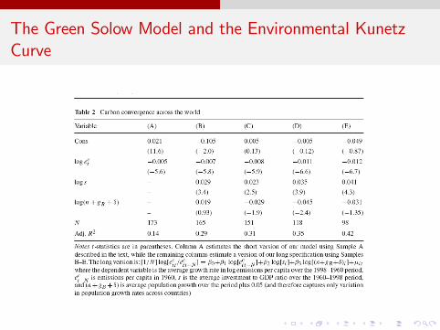
The Green Solow Model and the Environmental KunetzCurve
The econometric results reported by Brock and Taylor (2010) in Table2 show that
1 the coe¢ cient on lneCis negative and statistically signicant across
countries. Thus conditional convergence in per capita emissionsemerges.
2 The coe¢ cient on ln(s) is positive and the coe¢ cient on ln(n+ g + d)is negative, as predicted by the green Solow model.