Rain - PE1RQM effect.pdf · above 10 GHz - and often the studies of Mie scattering were incomplete...
30
________________________________ Effects of Rain on Propagation, Absorption and Scattering of Microwave Radiation Based on the Dielectric Model of Liebe Christian Mätzler ________________________________ Research Report No. 2002-10 June 2002 Institut für Angewandte Physik Mikrowellenabteilung __________________________________________________________ Sidlerstrasse 5 Tel. : +41 31 631 89 11 3012 Bern Fax. : +41 31 631 37 65 Schweiz E-mail : [email protected]
-
Upload
nguyennhan -
Category
Documents
-
view
213 -
download
0
Transcript of Rain - PE1RQM effect.pdf · above 10 GHz - and often the studies of Mie scattering were incomplete...

________________________________
Effects of Rain on Propagation, Absorption and Scatteringof Microwave Radiation Based on the Dielectric Model of
Liebe
Christian Mätzler
________________________________
Research Report No. 2002-10June 2002
Institut für Angewandte Physik Mikrowellenabteilung__________________________________________________________
Sidlerstrasse 5 Tel. : +41 31 631 89 113012 Bern Fax. : +41 31 631 37 65Schweiz E-mail : [email protected]

1
Effects of Rain on Propagation, Absorption and Scatteringof Microwave Radiation Based on the Dielectric Model of
Liebe
Christian Mätzler, Institute of Applied Physics, University of Bern, June 2002
List of ContentsAbstract..............................................................................................................11 Introduction.....................................................................................................22 Single water droplets........................................................................................3
2.1 Mie Efficiencies.............................................................................................................. 32.2 Comparison with Rayleigh Theory................................................................................. 32.3 Comparison between Liebe’91 and Liebe’93 ................................................................. 32.5 Angular diagrams and the internal field.......................................................................... 7
3 Clouds of rain drops ......................................................................................103.1 Transformation from efficiencies to coefficients............................................................ 103.2 Weighting functions of coefficients................................................................................ 103.3 Rain spectra .................................................................................................................... 143.4 Rain-rate dependence...................................................................................................... 143.4 Temperature dependence ................................................................................................ 14
4 Conclusions...................................................................................................25References ........................................................................................................25Appendix: The main MATLAB Functions............................................................26
A1 epswater .......................................................................................................................... 26A2 Mie_rain1........................................................................................................................ 26A3 Mie_rain2........................................................................................................................ 26A4 Mie_rain3........................................................................................................................ 27A5 Mie_rain4........................................................................................................................ 28
AbstractThis report presents results from Mie computations for extinction, scattering,absorption, backscattering, asymmetry parameter and angular scattering behaviourof microwave radiation by rain, based on a recently developed MATLAB software,and using two versions of the dielectric model of water by Liebe. The results are alsoquantitatively compared with results from Rayleigh Theory. The report contains thecode of the MATLAB routines.

2
1 IntroductionMie Theory (Mie, 1908), known for almost one century, allows for exact modelling ofwave propagation, absorption and scattering characteristics of spheres and ofclouds of such particles, provided that the dielectric and magnetic properties of theparticle are known. Water droplets of rain and clouds are nearly spherical, homo-geneous, dielectric particles, thus Mie Theory is quite appropriate for applications inatmospheric physics. Mie Theory has also been widely used for this purpose (e.g.Deirmendjian, 1969) to complement the results of Rayleigh scattering which are amuch simpler formulation, but applicable for small size parameters (x=ak<<1, a=drop radius, k= wave number) only. Most published studies usually relied on olddielectric data, such as Ray (1972) - being especially inaccurate at frequenciesabove 10 GHz - and often the studies of Mie scattering were incomplete descriptionsby considering one or another aspect, only; e.g. Olsen et al. (1978) gave aquantitative description of extinction by rain. Olsen’s result were of recent interest(Mätzler 2002a) to quantify rain effects on radar signals.A useful set of parameters, allowing a larger range of applications (wave propaga-tion, radiometer, monostatic radar), must include the extinction γext, absorption γabs,and backscattering coefficient γb, respectively, including the scattering coefficientγsca from γext-γabs; in addition, for modelling radiometer data with radiative transfertheory the full phase matrix is required as well or at least the asymmetry parameterg=<cosθ> if a simplified method is applied, such as the few-stream models (Meadorand Weaver, 1980). These parameters are computed and plotted by a set of MATLABFunctions, developed by Mätzler (2002b), based on the book of Bohren and Huffman(1983). The present report is an application of this software. The objective isthreefold:1. to extend the MATLAB functions to cloud and rain applications for general use
in the 1 to 1000 GHz range (or to the optical range with an appropriate refractivemodel of water),
2. to prepare our research group for microwave radiometry of the rainy atmos-phere,
3. to replace the rather inaccurate results of Olsen et al. (1978) by better ones andto complement them with more additional information.
Here, the presently assumed standard dielectric model of water will be applied(Liebe et al. 1991), and comparisons will be made with an alternative one (Liebe etal. 1993). At a temperature of 300K, the two models coincide. They deviate just inone parameter, the permittivity at infinite frequency,
+
=∞ )1993(.aletLiebe;52.3)1991(.aletLiebeθ;52.752.3
ε (1)
where θ =1-300/T, and T is the temperature in K. Thus at frequencies f near orbelow 30 GHz, the difference between the two models is negligible.The Marshall and Palmer (MP) drop-size distribution will be assumed:
)exp()( 0 DNDNMP Λ−= (2)
with the drop diameter D, the parameter Λ being given by (Sauvageot, 1992)
0/67.3 D=Λ = 21.041 −R (1/cm) (3)
where D0 (cm) is the median diameter, R (mm/h) the rain rate, and N0 = 0.08 cm-4.Olsen et al. (1978) and de Wolf (2001) proposed renormalisations of the MP distri-

3
bution to produce correct rain rates. Since these corrections are different, we willomit them here.
2 Single water droplets2.1 Mie EfficienciesMie Theory requires the complex refractive index of water m as input parameter.Since the relative magnetic permeability of water is very close to 1, we can assumethe relationship for non-magnetic materials
ε=m (4)
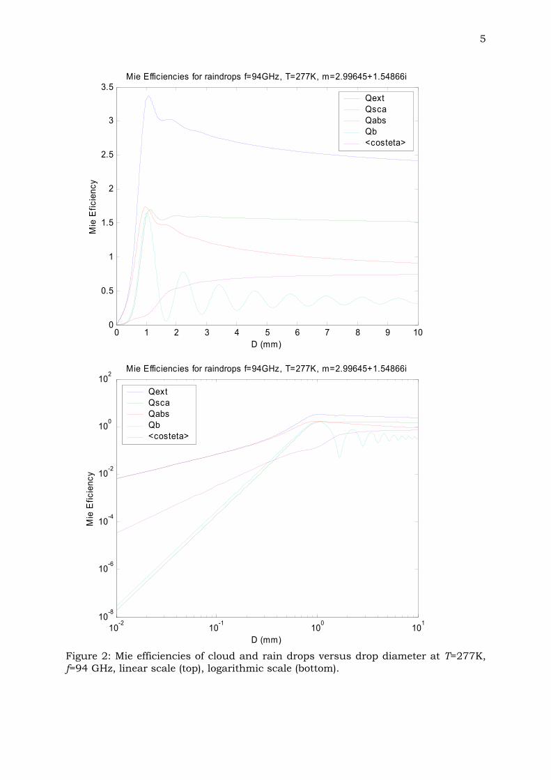
where ε is the complex relative dielectric constant (or permittivity) of liquid water.For ε we use the model of Liebe et al. (1991). The MATLAB function is calledepswater. For the alternative model, Liebe et al. (1993), the MATLAB Function iscalled epswater93.Mie Efficiencies of water droplets are computed at T=277K for two frequencies,using the MATLAB Function Mie_rain1. The results are shown versus drop diameterD in Figures 1 and 2. At the logarithmic scales, starting at D=10µm (a typical cloud-drop size), the figures emphasise the Rayleigh regime with straight lines up to about2 mm at 5 GHz and 0.3 mm at 94 GHz. This is the reason why rain-radar data at 5GHz (e.g. Sauvageot, 1992) are usually interpreted in terms of Rayleigh scatteringtheory (van de Hulst, 1957, Ishimaru, 1978).
2.2 Comparison with Rayleigh TheoryTo test the accuracy of the Rayleigh Approximation, the Mie and Rayleigh resultsare compared in Figure 3. It is observed that Rayleigh Theory underestimates ab-sorption at f=5GHz at D=2mm (x≅0.1) by a factor of 1/2 already, and computationswith an accuracy of 10% only reach to D=0.7 mm. For accurate modelling of micro-wave emission, absorption should be known to the 1% level. Thus Mie Theory isneeded in microwave radiometry of rain at 5 GHz and at all higher frequencies.For scattering and backscattering, on the other hand, the Rayleigh Approximationis valid (deviations < 25%) up to D=6 mm, thus covering the full range of rain drops.Since radar data are usually needed with an accuracy of about 1 dB (26%), theRayleigh Approximation is sufficient for radar observations at 5 GHz. Note theslightly oscillatory behaviour of the Mie backscattering efficiency around the Ray-leigh curve in Figure 3.Similar results are found at 94 GHz (bottom graph of Figure 3). The underestimateof absorption of the Rayleigh curve by a factor of 1/2 is reached at D=0.5 mm(x≅0.5), i.e. at a 4 times lower value of D than at 5 GHz, whereas the frequency ishigher by a factor of 19. This behaviour is due to the relaxation spectrum of water.Again for scattering, and especially for backscattering, the Rayleigh Approximationis useful up to higher D values, about 0.8 mm.
2.3 Comparison between Liebe’91 and Liebe’93The two dielectric models, Liebe et al. (1991) and Liebe et al. (1993), give slightlydifferent results. The difference increases with increasing frequency and with tem-perature decreasing from 300 K. Mie efficiencies and their differences between thetwo dielectric models at 277K are shown in Figure 4 for f=24 and 220 GHz, respec-

4
tively. The differences are well below 0.001 at 24 GHz, whereas the efficiencies areon the order of 1. At 220 GHz, on the other hand, the differences
0 1 2 3 4 5 6 7 8 9 10-0.4
-0.2
0
0.2
0.4
0.6
0.8
1
1.2Mie Efficiencies for raindrops f=5GHz, T=277K, m=8.60899+1.84624i
D (mm)
Mie
Efic
ienc
y
QextQscaQabsQb<costeta>
10-2 10-1 100 10110-14
10-12
10-10
10-8
10-6
10-4
10-2
100
102Mie Efficiencies for raindrops f=5GHz, T=277K, m=8.60899+1.84624i
D (mm)
Mie
Efic
ienc
y
QextQscaQabsQb<costeta>
Figure 1: Mie efficiencies of cloud and rain drops versus drop diameter at T=277K,f=5 GHz, linear scale (top), logarithmic scale (bottom).
5
0 1 2 3 4 5 6 7 8 9 100
0.5
1
1.5
2
2.5
3
3.5Mie Efficiencies for raindrops f=94GHz, T=277K, m=2.99645+1.54866i
D (mm)
Mie
Efic
ienc
yQextQscaQabsQb<costeta>
10-2 10-1 100 10110-8
10-6
10-4
10-2
100
102Mie Efficiencies for raindrops f=94GHz, T=277K, m=2.99645+1.54866i
D (mm)
Mie
Efic
ienc
y
QextQscaQabsQb<costeta>
Figure 2: Mie efficiencies of cloud and rain drops versus drop diameter at T=277K,f=94 GHz, linear scale (top), logarithmic scale (bottom).

6
1 2 3 4 5 6 7 8 9 10
10-4
10-3
10-2
10-1
100Mie and Rayleigh Efficiencies of raindrops f=5GHz, T=277K
D (mm)
Mie
Efic
ienc
y
QscaMQscaRQabsMQabsRQbMQbR
0 0.1 0.2 0.3 0.4 0.5 0.6 0.7 0.8 0.9 10
0.2
0.4
0.6
0.8
1
1.2
1.4
1.6
1.8
2Mie and Rayleigh Efficiencies of raindrops f=94GHz, T=277K
D (mm)
Mie
Efic
ienc
y
QscaMQscaRQabsMQabsRQbMQbR
Figure 3: Mie Efficiencies of water drops versus drop diameter in Mie (M) and Ray-leigh (R) Theory at T=277K, f= 5 (top) and 94 GHz (bottom), respectively.

7
0 1 2 3 4 5 6 7 8 9 10-0.5
0
0.5
1
1.5
2
2.5
3
3.5Mie Efficiencies for raindrops f=24GHz, T=277K, m=5.12255+2.84771i
D (mm)
Mie
Efic
ienc
y
QextQscaQabsQb<costeta>
0 1 2 3 4 5 6 7 8 9 10-8
-6
-4
-2
0
2
4
6
8
10x 10-4 f=24GHz, T=277K, m91-m93 = 0.00135988+0.00282742i
D (mm)
Mie
Efic
ienc
y D
iffer
ence
s Li
ebe9
1-Li
ebe9
3
dQextdQscadQabsdQbd<costeta>
0 0.5 1 1.5 2 2.5 30
0.5
1
1.5
2
2.5
3
3.5Mie Efficiencies for raindrops f=220GHz, T=277K, m=2.50551+0.98578i
D (mm)
Mie
Efic
ienc
y
QextQscaQabsQb<costeta>
0 0.5 1 1.5 2 2.5 3-0.03
-0.02
-0.01
0
0.01
0.02
0.03
0.04
0.05
0.06f=220GHz, T=277K, m91-m93 = -0.00721301+0.0548145i
D (mm)
Mie
Efic
ienc
y D
iffer
ence
s Li
ebe9
1-Li
ebe9
3
dQextdQscadQabsdQbd<costeta>
Figure 4: Mie Efficiencies at 24 (upper left) and 220 GHz (lower left) versus dropdiameter at T=277K, and (right) the differences between the two dielectric models,Liebe et a. (1991) – Liebe et al. (1993).
are on the order of 0.01, reaching up to 0.05. Still these differences do not deviateby more than 1% or a few %. Therefore, from here on, we will neglect the differencesbetween the two models, by using Liebe‘91 only.
2.5 Angular diagrams and the internal fieldScattering diagrams of water droplets with increasing D are shown for f=94 GHz inthe graphs of Figure 5. While the scattering efficiency is nearly constant at about1.6 for the three situations (s. Figure 2), there is a strong change from near-iso-tropic scattering at x=1 to forward scattering at x=2.2. This change is indicated inFigure 2 by the increase of <cosθ> over the considered range of x. The top graph ofFigure 5 is the situation with maximum backscattering Qb, the middle graph showsa situation with reduced Qb, and the bottom graph corresponds to the secondmaximum of Qb in Figure 2. While the monostatic radar signal from rain is notdirectly influenced by the changing scattering diagram, the modeling of microwaveemission depends on the angular diagram, i.e. on the phase function (Chandrasek-har, 1960; Ishimaru, 1978).

8
0.2
0.4
0.6
0.8
1
30
210
60
240
90
270
120
300
150
330
180 0
Mie angular scattering: m=2.99645+1.54866i, x=1
Scattering Angle
Figure 5: Angular diagrams forMie scattering on raindrops atf=94 GHz, T=277K,top: x=1 (D=1.02 mm),middle: x=1.5 (D=1.52 mm),bottom: x=2.2 (D=2.23 mm).
The upper part of the curves(angular range 0-180°) are forpolarization perpendicular tothe scattering plane, and thelower part of the curves (angu-lar range 180-360°) are for po-larization parallel to the scat-tering plane.
1
2
3
30
210
60
240
90
270
120
300
150
330
180 0
Mie angular scattering: m=2.99645+1.54866i, x=1.5
Scattering Angle
5
10
15
30
210
60
240
90
270
120
300
150
330
180 0
Mie angular scattering: m=2.99645+1.54866i, x=2.2
Scattering Angle

9
0 0.1 0.2 0.3 0.4 0.5 0.6 0.7 0.8 0.9 10.125
0.13
0.135
0.14
0.145
0.15
0.155
0.16
0.165
0.17Squared Amplitude E Field in a Sphere, m=2.99645+1.54866i, x=1
r k
Radial Dependence of (abs(E))2
Figure 6: Radial dependence ofmean-absolute-square electricfield ratio between inside araindrop and the incident fieldfor Mie scattering at f=94 GHz,T=277K,top: x=1 (D=1.02 mm),middle: x=1.5 (D=1.52 mm),bottom: x=2.2 (D=2.23 mm).
0 0.5 1 1.50
0.02
0.04
0.06
0.08
0.1
0.12
Squared Amplitude E Field in a Sphere, m=2.99645+1.54866i, x=1.5
r k
Radial Dependence of (abs(E))2
0 0.5 1 1.5 20
0.02
0.04
0.06
0.08
0.1
0.12Squared Amplitude E Field in a Sphere, m=2.99645+1.54866i, x=2.2
r k
Radial Dependence of (abs(E))2
The ratio of the absolute-squareelectric field between the insideof the sphere and the incidentfield is shown here in thegraphs of Figure 6 versus the k-normalised radial distance r forthe 3 situations of Figure 5. Thevalues are averaged over shellsof constant radius.It is seen that already at x=1the internal field is significantlylarger than in case of Rayleighscattering; in the Rayleigh limit,the value follows from
22 2/9 +m , thus becomes
0.056. This is the reason for theenhanced absorption in MieTheory for small values of x(here x=1).At the bottom graph, the field isconcentrated at the edge of thedrop due to the skin effect.

10
3 Clouds of rain drops3.1 Transformation from efficiencies to coefficientsFor a large number of independently and incoherently scattering rain drops dis-tributed in air (assuming the refractive index of air being 1), the propagation coeffi-cients (extinction γext, scattering γsca, backscattering γb and absorption γabs coeffi-cients) are determined from the Mie efficiencies and the drop-size distribution by
∫∞
=0
2 )()(25.0 dDdNDQD MPjj πγ ; j = ext, abs, sca, b (5)
∫∞
⋅><=0
2 )()()(cos25.0cos dDdNDQDD MPscasca θπθγ (6)
where <cosθ>(D) is a function of D; the dimension of the coefficients is 1/(length) asthey represent densities of cross sections. Here we will use 1/km or, what is identi-cal, neper/km. The transformation to dB/km is obtained by multiplying the γj val-ues with 10⋅10loge ≅ 0.4342. These coefficients are used in radiative transfer theory(Chandrasekhar, 1960, Meador and Weaver, 1980).
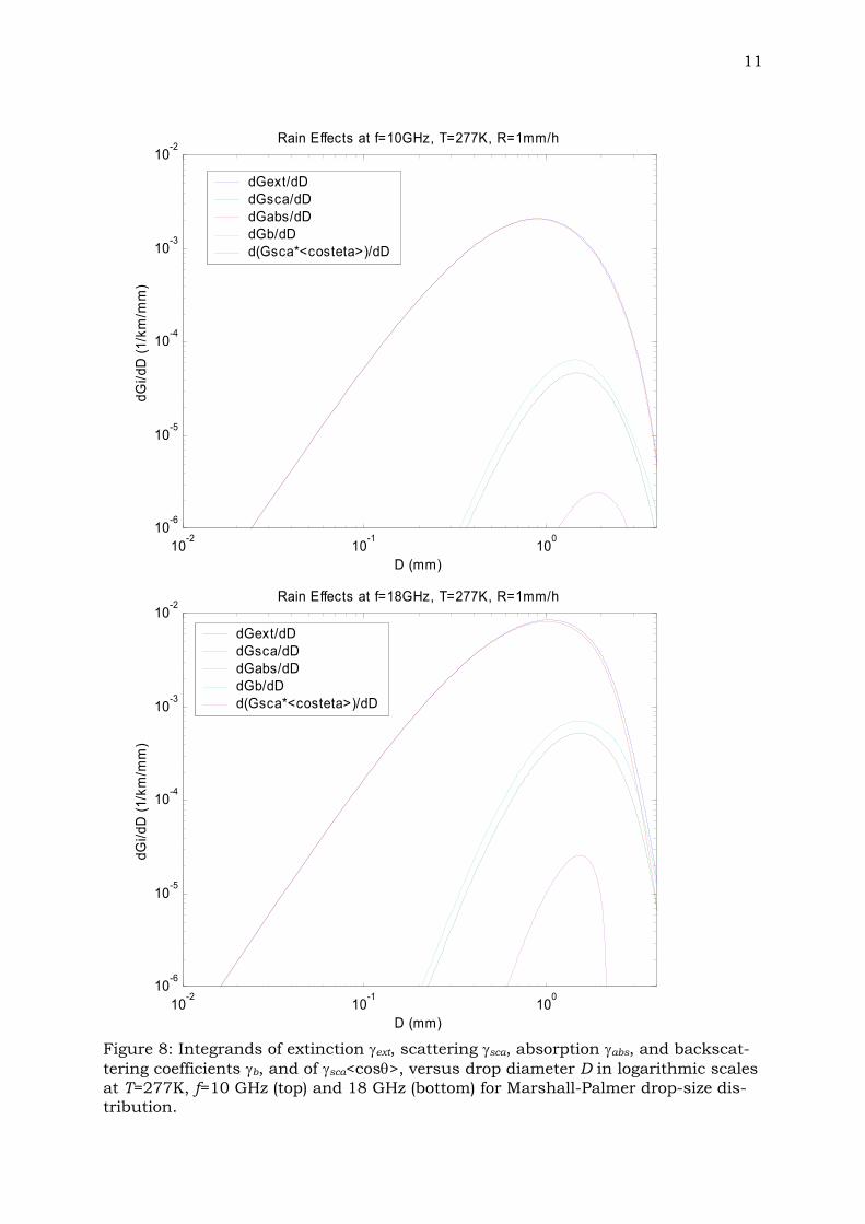
3.2 Weighting functions of coefficientsThe integrands of γj can be considered as weighting functions in the averaging overD. The strong exponential decrease of NMP with increasing D gives a strong weightingof small droplets. On the other hand, the efficiencies of zero-sized droplets are zeroand increase, according to the Rayleigh Approximation, in proportion to D2 forabsorption and D6 for scattering. Thus, there is a D range of maximum influence,depending on the parameter in question, and with a strong sensitivity to frequency.Different situations are shown in the following figures, based on the MATLAB Func-tion Mie_rain2. At frequencies up to 10 GHz, scattering is negligible in comparisonto absorption. An example with f=5 GHz is shown in Figure 7. To better see thescattering effects, logarithmic scales are used in Figure 8, showing data at 10 and18 GHz.
0 1 2 3 4 5 6 7-0.5
0
0.5
1
1.5
2
2.5x 10⁻³ Rain Effects at f=5GHz, T=277K, R=10mm/h
D (mm)
dGi/d
D (1
/km
/mm
)
dGext/dDdGsca/dDdGabs/dDdGb/dDd(Gsca*<costeta>)/dD
Figure 7:Integrands of γj at f=5GHz, T=277K.
11
10-2 10-1 10010-6
10-5
10-4
10-3
10-2Rain Effects at f=10GHz, T=277K, R=1mm/h
D (mm)
dGi/d
D (1
/km
/mm
)
dGext/dDdGsca/dDdGabs/dDdGb/dDd(Gsca*<costeta>)/dD
10-2 10-1 10010-6
10-5
10-4
10-3
10-2Rain Effects at f=18GHz, T=277K, R=1mm/h
D (mm)
dGi/d
D (1
/km
/mm
)
dGext/dDdGsca/dDdGabs/dDdGb/dDd(Gsca*<costeta>)/dD
Figure 8: Integrands of extinction γext, scattering γsca, absorption γabs, and backscat-tering coefficients γb, and of γsca<cosθ>, versus drop diameter D in logarithmic scalesat T=277K, f=10 GHz (top) and 18 GHz (bottom) for Marshall-Palmer drop-size dis-tribution.
12
0 0.5 1 1.5 2 2.5 3 3.5 4-0.005
0
0.005
0.01
0.015
0.02
0.025
0.03
0.035
0.04
0.045Rain Effects at f=35GHz, T=277K, R=1mm/h
D (mm)
dGi/d
D (1
/km
/mm
)
dGext/dDdGsca/dDdGabs/dDdGb/dDd(Gsca*<costeta>)/dD
0 0.5 1 1.5 2 2.5 3 3.5 40
0.05
0.1
0.15
0.2
0.25
0.3
0.35
0.4Rain Effects at f=94GHz, T=277K, R=1mm/h
D (mm)
dGi/d
D (1
/km
/mm
)
dGext/dDdGsca/dDdGabs/dDdGb/dDd(Gsca*<costeta>)/dD
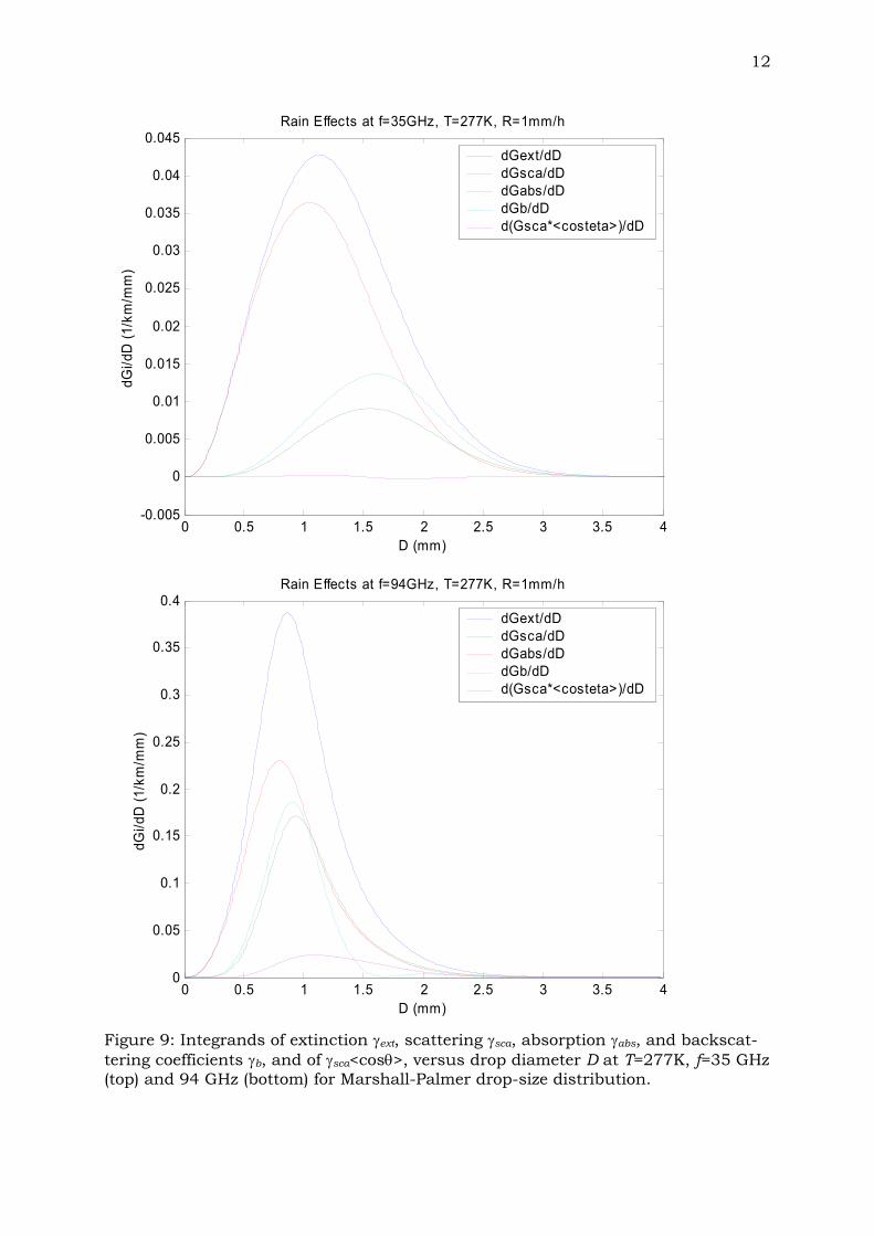
Figure 9: Integrands of extinction γext, scattering γsca, absorption γabs, and backscat-tering coefficients γb, and of γsca<cosθ>, versus drop diameter D at T=277K, f=35 GHz(top) and 94 GHz (bottom) for Marshall-Palmer drop-size distribution.

13
0 0.5 1 1.5 2 2.5 3 3.5 40
0.1
0.2
0.3
0.4
0.5
0.6
0.7Rain Effects at f=160GHz, T=277K, R=1mm/h
D (mm)
dGi/d
D (1
/km
/mm
)dGext/dDdGsca/dDdGabs/dDdGb/dDd(Gsca*<costeta>)/dD
0 0.5 1 1.5 2 2.5 3 3.5 40
0.1
0.2
0.3
0.4
0.5
0.6
0.7Rain Effects at f=300GHz, T=277K, R=1mm/h
D (mm)
dGi/d
D (1
/km
/mm
)
dGext/dDdGsca/dDdGabs/dDdGb/dDd(Gsca*<costeta>)/dD
Figure 10: Integrands of extinction γext, scattering γsca, absorption γabs, and backscat-tering coefficients γb, and of γsca<cosθ>, versus drop diameter D at T=277K, f=160GHz (top) and 300 GHz (bottom) for Marshall-Palmer drop-size distribution.
14
Figures 9 and 10, again with linear scales, represent the behaviour at frequenciesfrom 31 to 300 GHz. It is interesting to note that the functions shown in Figures 7to 10 are clearly peaked ones. This is especially true for the backscattering coeffi-cient γb. It means that a multi-frequency radar can give detailed information on thedrop-size distribution. Reasons why radar systems have - so far - not been used forthis purpose, may be related to the inherent noise (e.g. speckle, clutter) in the data,and in the high extinction at mm wavelengths.The maximum of the weighting for γb is near D=2.2 mm at 5 GHz, almost constantnear 1.5 mm at 10 to 35 GHz, at 1mm near 94 GHz, at 0.6 mm at 160 GHz and 0.3mm at 300 GHz. Thus the typical drop-size range is covered by these frequencies.Note that the weighting functions of other parameters are slightly different. Theasymmetry parameter has sometimes slightly negative values, indicating increasedscattering in the backward hemisphere. But more often the values are positive.
3.3 Rain spectraThe results of the integration of the Mie Efficiencies over the drop-size distributionleads to the propagation coefficients, using the MATLAB Function Mie_rain3. Carehas to be taken to select the best range of D values. The following parameters werefound to be useful and to give accurate results with trapezoidal integration:
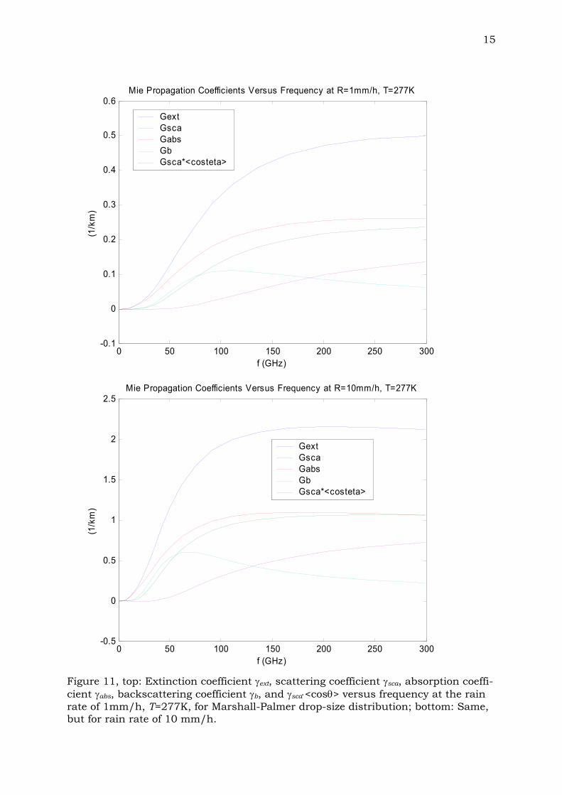
nsteps=501; dD=0.01*R^(1/6)/fGHz^0.05; (7)where nsteps is the number of steps in the numerical integration, starting at D=0,and dD is the increment in dependence on rain rate R(mm/h) and frequency fGHz(GHz).The γj spectra of rain at 277K are shown in Figure 11 for rain rates R of 1 and 10mm/h. These curves tend to increase with increasing frequency, either reachingsaturation at the top or above the presented spectral range or a flat peak, especiallyfor γb. The peak frequency decreases with increasing rain rate. Another feature isthe decreasing dominance of absorption with increasing frequency and rain rate.
3.4 Rain-rate dependenceThe γj coefficients are shown versus rain rate, both in linear and logarithmic scalesin Figures 12 to 17. These are quite smooth curves in both representations, some-times being almost straight lines.The extinction coefficients can be used to check the approximate formula of Olsenet al. (1978), γext ≅ αRβ, where α and β depend on frequency, drop-size distributionand temperature. For T=0, 10 and 20C, and for the dielectric water model of Ray(1972), these parameters were given by Olson et al. (1978), and the tables arereprinted by Mätzler (2002a). However, when looking at Figures 12 to 17, it is clearthat the Olsen formula cannot be very accurate as it require strait lines in the loga-rithmic representations. Therefore Olsen’s fits represent rough approximations ofextinction, only.
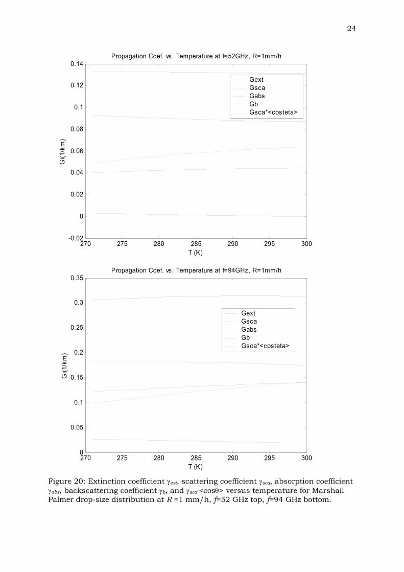
3.4 Temperature dependenceThe dependence of the propagation coefficients on temperature is shown by Figures18 to 20, covering the frequency range, 5 to 94 GHz. The maximum sensitivity isfound for absorption at the lowest frequency; this is a result of the rather strongtemperature dependence of the lower relaxation frequency.
15
0 50 100 150 200 250 300-0.1
0
0.1
0.2
0.3
0.4
0.5
0.6Mie Propagation Coefficients Versus Frequency at R=1mm/h, T=277K
f (GHz)
(1/k
m)
GextGscaGabsGbGsca*<costeta>
0 50 100 150 200 250 300-0.5
0
0.5
1
1.5
2
2.5Mie Propagation Coefficients Versus Frequency at R=10mm/h, T=277K
f (GHz)
(1/k
m)
GextGscaGabsGbGsca*<costeta>
Figure 11, top: Extinction coefficient γext, scattering coefficient γsca, absorption coeffi-cient γabs, backscattering coefficient γb, and γsca⋅<cosθ> versus frequency at the rainrate of 1mm/h, T=277K, for Marshall-Palmer drop-size distribution; bottom: Same,but for rain rate of 10 mm/h.

16
0 10 20 30 40 50 60 70 80 90 1000
0.01
0.02
0.03
0.04
0.05
0.06
0.07
0.08
0.09
0.1Mie Propagation Coefficients Versus Rain Rate at f=5GHz, T=277K
R (mm/h)
(1/k
m)
GextGscaGabsGbGsca*<costeta>
10-1 100 101 10210-9
10-8
10-7
10-6
10-5
10-4
10-3
10-2
10-1Mie Propagation Coefficients Versus Rain Rate at f=5GHz, T=277K
R (mm/h)
(1/k
m)
GextGscaGabsGbGsca*<costeta>
Figure 12, top: Extinction coefficient γext, scattering coefficient γsca, absorption coeffi-cient γabs, backscattering coefficient γb, and γsca⋅<cosθ> versus rain rate at T=277K,f=5GHz for Marshall-Palmer drop-size distribution. Linear scales; bottom: Same, butlogarithmic scales.

17
0 10 20 30 40 50 60 70 80 90 100-0.1
0
0.1
0.2
0.3
0.4
0.5
0.6
0.7Mie Propagation Coefficients Versus Rain Rate at f=10GHz, T=277K
R (mm/h)
(1/k
m)
GextGscaGabsGbGsca*<costeta>
10-1 100 101 10210-6
10-5
10-4
10-3
10-2
10-1
100Mie Propagation Coefficients Versus Rain Rate at f=10GHz, T=277K
R (mm/h)
(1/k
m)
GextGscaGabsGb
Figure 13, top: Extinction coefficient γext, scattering coefficient γsca, absorption coeffi-cient γabs, backscattering coefficient γb, and γsca⋅<cosθ> versus rain rate at T=277K,f=10GHz for Marshall-Palmer drop-size distribution. Linear scales; bottom: Same,without γsca⋅<cosθ>, logarithmic scales.

18
0 10 20 30 40 50 60 70 80 90 100-0.5
0
0.5
1
1.5
2
2.5Mie Propagation Coefficients Versus Rain Rate at f=18GHz, T=277K
R (mm/h)
(1/k
m)
GextGscaGabsGbGsca*<costeta>
10-1 100 101 10210-5
10-4
10-3
10-2
10-1
100
101Mie Propagation Coefficients Versus Rain Rate at f=18GHz, T=277K
R (mm/h)
(1/k
m)
GextGscaGabsGb
Figure 14, top: Extinction coefficient γext, scattering coefficient γsca, absorption coeffi-cient γabs, backscattering coefficient γb, and γsca⋅<cosθ> versus rain rate at T=277K,f=18GHz for Marshall-Palmer drop-size distribution. Linear scales; bottom: Same,without γsca⋅<cosθ>, logarithmic scales.

19
0 10 20 30 40 50 60 70 80 90 100-1
0
1
2
3
4
5Mie Propagation Coefficients Versus Rain Rate at f=31.4GHz, T=277K
R (mm/h)
(1/k
m)
GextGscaGabsGbGsca*<costeta>
10-1 100 101 10210-4
10-3
10-2
10-1
100
101Mie Propagation Coefficients Versus Rain Rate at f=31.4GHz, T=277K
R (mm/h)
(1/k
m)
GextGscaGabsGb
Figure 15, top: Extinction coefficient γext, scattering coefficient γsca, absorption coeffi-cient γabs, backscattering coefficient γb, and γsca⋅<cosθ> versus rain rate at T=277K,f=31.4GHz for Marshall-Palmer drop-size distribution. Linear scales; bottom: Same,without γsca⋅<cosθ>, logarithmic scales.

20
0 10 20 30 40 50 60 70 80 90 1000
1
2
3
4
5
6
7
8Mie Propagation Coefficients Versus Rain Rate at f=52GHz, T=277K
R (mm/h)
(1/k
m)
GextGscaGabsGbGsca*<costeta>
10-1 100 101 10210-3
10-2
10-1
100
101Mie Propagation Coefficients Versus Rain Rate at f=52GHz, T=277K
R (mm/h)
(1/k
m)
GextGscaGabsGb
Figure 16, top: Extinction coefficient γext, scattering coefficient γsca, absorption coeffi-cient γabs, backscattering coefficient γb, and γsca⋅<cosθ> versus rain rate at T=277K,f=52 GHz for Marshall-Palmer drop-size distribution. Linear scales; bottom: Same,without γsca⋅<cosθ>, logarithmic scales.
21
0 10 20 30 40 50 60 70 80 90 1000
1
2
3
4
5
6
7
8
9
10Mie Propagation Coefficients Versus Rain Rate at f=94GHz, T=277K
R (mm/h)
(1/k
m)
GextGscaGabsGbGsca*<costeta>
10-1 100 101 10210-2
10-1
100
101Mie Propagation Coefficients Versus Rain Rate at f=94GHz, T=277K
R (mm/h)
(1/k
m)
GextGscaGabsGb
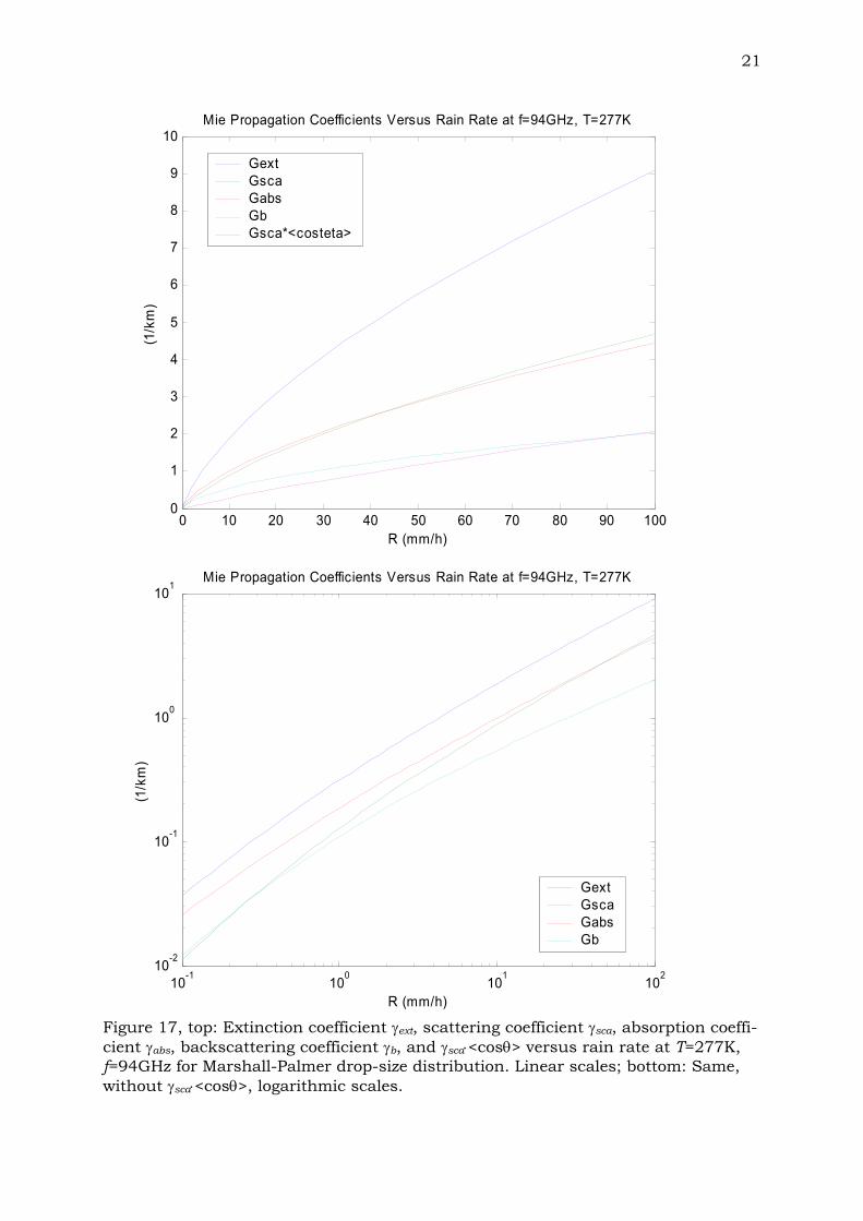
Figure 17, top: Extinction coefficient γext, scattering coefficient γsca, absorption coeffi-cient γabs, backscattering coefficient γb, and γsca⋅<cosθ> versus rain rate at T=277K,f=94GHz for Marshall-Palmer drop-size distribution. Linear scales; bottom: Same,without γsca⋅<cosθ>, logarithmic scales.

22
270 275 280 285 290 295 3000
2
4
6
8x 10⁻⁴ Propagation Coef. vs. Temperature at f=5GHz, R=1mm/h
T (K)
Gi(1
/km
)GextGscaGabsGbGsca*<costeta>
270 275 280 285 290 295 3000
0.5
1
1.5
2
2.5
3
3.5x 10⁻³ Propagation Coef. vs. Temperature at f=10GHz, R=1mm/h
T (K)
Gi(1
/km
)
GextGscaGabsGbGsca*<costeta>
Figure 18: Extinction coefficient γext, scattering coefficient γsca, absorption coefficientγabs, backscattering coefficient γb, and γsca⋅<cosθ> versus temperature for Marshall-Palmer drop-size distribution at R =1 mm/h, f=5 GHz top, f=10 GHz bottom.

23
270 275 280 285 290 295 3000
0.002
0.004
0.006
0.008
0.01
0.012
0.014 Propagation Coef. vs. Temperature at f=18GHz, R=1mm/h
T (K)
Gi(1
/km
)
GextGscaGabsGbGsca*<costeta>
270 275 280 285 290 295 300-0.01
0
0.01
0.02
0.03
0.04
0.05 Propagation Coef. vs. Temperature at f=31.4GHz, R=1mm/h
T (K)
Gi(1
/km
)
GextGscaGabsGbGsca*<costeta>
Figure 19: Extinction coefficient γext, scattering coefficient γsca, absorption coefficientγabs, backscattering coefficient γb, and γsca⋅<cosθ> versus temperature for Marshall-Palmer drop-size distribution at R =1 mm/h, f=18 GHz top, f=31.4 GHz bottom.
24
270 275 280 285 290 295 300-0.02
0
0.02
0.04
0.06
0.08
0.1
0.12
0.14 Propagation Coef. vs. Temperature at f=52GHz, R=1mm/h
T (K)
Gi(1
/km
)
GextGscaGabsGbGsca*<costeta>
270 275 280 285 290 295 3000
0.05
0.1
0.15
0.2
0.25
0.3
0.35 Propagation Coef. vs. Temperature at f=94GHz, R=1mm/h
T (K)
Gi(1
/km
)
GextGscaGabsGbGsca*<costeta>
Figure 20: Extinction coefficient γext, scattering coefficient γsca, absorption coefficientγabs, backscattering coefficient γb, and γsca⋅<cosθ> versus temperature for Marshall-Palmer drop-size distribution at R =1 mm/h, f=52 GHz top, f=94 GHz bottom.

25
4 ConclusionsThis report is a graphical presentation of results from Mie Theory of rain in the mi-crowave and millimeter wavelength range. The presentation is as comprehensive aspossible by giving all relevant parameters and showing all relevant dependencies.The graphs are instructive in the sense that they show how the different parametersbehave, how they are related quantitatively and which drop-sizes contribute most.In addition, the results show that the limits of Rayleigh Theory are not just at a sizeparameter of x=1, as often stated. The absorption coefficient can be stronglyunderestimated by the Rayleigh Approximation at x=0.1 already. On the other hand,weaker deviations are found for the scattering parameters at this x range; however,for large x, they diverge much more strongly than the absorption coefficient.To apply and extend the presented data, the reader is encouraged to use theMATLAB Functions given in the Appendix.
References
Bohren C.F. and D.R. Huffman, “Absorption and Scattering of Light by Small Particles”, John Wiley,New York, NY (1983).
Chandrasekhar S., "Radiative Transfer", Dover Publication (1960), BEWI TDD 211.Deirmendjian, D. “Electromagnetic Scattering on Spherical Polydispersions”, American Elsevier, New
York, NY (1969).de Wolf D.A. “On the Laws-Parsons distribution of raindrop sizes”, Radio Science Vol.36, No. 4, pp.
639-642 (2001).Ishimaru A., “Wave propagation and scattering in random media”, Vol. 1, Academic Press, Orlando,
FL (1978).Liebe H.J., G.A. Hufford and T. Manabe, “A model for the complex permittivity of water at frequencies
below 1 THz”, Internat. J. Infrared and mm Waves, Vol. 12, pp. 659-675 (1991).Liebe, H.J., G.A. Hufford, and M.G. Cotton, Propagation Modeling of Moist Air and Suspended
Water/Ice Particles at Frequencies Below 1000 GHz. AGARD Conference Proc. 542, AtmosphericPropagation Effects through Natural and Man-Made Obscurants for Visible to MM-Wave Radiation,pp.3.1-3.10 (1993).
Math Works, “MATLAB User’s Guide”, Natick, MA (1992).Mätzler C., “Radarsignale von anisotropem Niederschlag ”, IAP Res. Rep. No. 02-2, April (2002a).Mätzler C., “MATLAB Functions for Mie Scattering and Absorption”, IAP Res. Rep. No. 02-08, June
(2002b).Mie G. “Beiträge zur Optik trüber Medien, speziell kolloidaler Metallösungen“, Annals of Physics, Vol.
25, pp. 377-445 (1908).Meador W.E. and W.R. Weaver, “Two-Stream Approximations to Radiative Transfer in Planetary
Atmospheres: A Unified Description of Existing Methods and a New Improvement”, J. Atm. Sci-ences, Vol. 37, pp. 630-643 (1980).
Olsen R.L., D.V. Rogers and D.B. Hodge, “The aRb relation in the calculation of rain attenuation”,IEEE Trans. Ant. Prop. Vol. AP-26, pp. 318-329 (1978).
Ray P.S. “Broadband complex refractive indices of ice and water”, Applied Optics, Vol. 11, No. 8, pp.1836-1844 (1972).
Sauvageot H., “Radar Meteorology”, Artech House, Boston, MA (1992).van de Hulst H.C. “Light Scattering by Small Particles”, (1957), reprinted by Dover Publication, New
York, NY (1981).

26
Appendix: The main MATLAB FunctionsThis appendix contains the main MATLAB routines used in this report. The routinesmake use of the Mie Functions defined elsewhere (Mätzler 2002b). Some additionalroutines are slight modifications of the ones shown here, e.g. to plot thetemperature dependence of the coefficients or to compare with Rayleigh Theory.
A1 epswaterfunction result = epswater(fGHz, TK)
% Dielectric permittivity of liquid water without salt according to Liebe et al. 1991 Int. J. IR+mm Waves 12(12), 659-675% Frequency range: 1 to 1000 GHz, temperature range: 270 to 310 K, extended 250 to 330 K% Input: fGHz: frequency in GHz, TK: temperature in K% Mätzler, June 2002
TETA=1-300/TK;e0=77.66-103.3*TETA;e1=0.0671*e0;f1=20.2+146.4*TETA+316*TETA.*TETA;e2=3.52+7.52*TETA;% version of Liebe 1993 uses: e2=3.52f2=39.8*f1;eps=e2+(e1-e2)./(1-i*fGHz./f2)+(e0-e1)./(1-i*fGHz./f1);result=eps;
A2 Mie_rain1function result = Mie_rain1(fGHz, TK, nsteps, dD)
% Efficiencies of rain extinction, scattering, absorption backscattering and asymmetric scattering, using Mie Theory and% the dielectric model of Liebe et al. (1991), see epswater.% Input: fGHz frequency in GHz, TK temperature in K, nsteps number of diameters (D in mm), dD increment of D in mm% C. Mätzler, June 2002
m=sqrt(epswater(fGHz, TK));nx=(1:nsteps)';D=(nx-1)*dD;c0=299.793;x=pi*D*fGHz/c0;for j = 1:nsteps a(j,:)=Mie(m,x(j));end;output_parameters='Real(m), Imag(m), D, Qext, Qsca, Qabs, Qb, <costeta>'a(:,3)=D;m1=real(m);m2=imag(m);plot(a(:,3),a(:,4:8)) % plotting the resultslegend('Qext','Qsca','Qabs','Qb','<costeta>')title(sprintf('Mie Efficiencies for raindrops f=%gGHz, T=%gK,m=%g+%gi',fGHz,TK,m1,m2))xlabel('D (mm)'), ylabel('Mie Efficiency')result=a;
A3 Mie_rain2function result = Mie_rain2(fGHz, TK, R)
% Weighting functions of Rain extinction, scattering, absorption, backscattering and asymmetric scattering coefficient

27
% in 1/km/mm versus drop diameter for Marshall-Palmer (MP) size distribution (Sauvageot et al. 1992)% using Mie Theory, and dielectric model of Liebe et al. 1991. Input:% fGHz: frequency in GHz, TK: Temp. in K, R: rain rate in mm/h% C. Mätzler, June 2002.
nsteps=501; dD=0.01*R^(1/6)/fGHz^0.05;% nsteps: number of D values, dD: drop-size interval in mmm=sqrt(epswater(fGHz, TK));N0=0.08/10000; % original MP N0 in 1/mm^4LA=4.1/R^0.21;nx=(1:nsteps)';D=(nx-1)*dD;c0=299.793;x=pi*D*fGHz/c0;sigmag=pi*D.*D/4;NMP=N0*exp(-LA*D);sn=sigmag.*NMP*1000000;for j = 1:nsteps a(j,:)=Mie(m,x(j));end;b(:,1)=D;b(:,2)=a(:,4).*sn;b(:,3)=a(:,5).*sn;b(:,4)=a(:,6).*sn;b(:,5)=a(:,7).*sn;b(:,6)=a(:,5).*a(:,8).*sn;m1=real(m);m2=imag(m);plot(b(:,1),b(:,2:6)) % plotting the resultslegend('dGext/dD','dGsca/dD','dGabs/dD','dGb/dD','d(Gsca*<costeta>)/dD')title(sprintf('Rain Effects at f=%gGHz, T=%gK, R=%gmm/h',fGHz,TK,R))xlabel('D (mm)');ylabel('dGi/dD (1/km/mm)')gext= sum(b(:,2))*dD;gsca= sum(b(:,3))*dD;gabs= sum(b(:,4))*dD;gb= sum(b(:,5))*dD;gteta=sum(b(:,6))*dD;result=[gext gsca gabs gb gteta];
A4 Mie_rain3function result = Mie_rain3(fGHz, TK, nrain, pam)
% Extinction, scattering, absorption, backscattering and asymmetric scattering coefficients in 1/km versus rain rate,% for Marshall-Palmer (MP) drop-size distribution (Sauvageot et al. 1992), using Mie Theory, and Liebe 91 dielectric model.% Input: fGHz: frequency in GHz, TK: Temp. in K, nrain: Number of rain rates between Rmin=0.1 and Rmax=100mm/h% pams: 0 if no costeta data to be given, 1 if they are needed% C. Mätzler, June 2002.
Rmin=0.1;nsteps=501;m=sqrt(epswater(fGHz, TK));N0=0.08/10000; % original MP N0 in 1/mm^4fact=1000^(1/(nrain-1));R=Rmin/fact;nx=(1:nsteps)';c0=299.793;for jr = 1:nrain R=R*fact; dD=0.01*R^(1/6)/fGHz^0.05; D=(nx-1)*dD;

28
x=pi*D*fGHz/c0; sigmag=pi*D.*D/4; LA=4.1/R^0.21; NMP=N0*exp(-LA*D); sn=sigmag.*NMP*1000000; for j = 1:nsteps a(j,:)=Mie(m,x(j)); end; b(:,1)=D; b(:,2)=a(:,4).*sn; b(:,3)=a(:,5).*sn; b(:,4)=a(:,6).*sn; b(:,5)=a(:,7).*sn; b(:,6)=a(:,5).*a(:,8).*sn; gext= sum(b(:,2))*dD; gsca= sum(b(:,3))*dD; gabs= sum(b(:,4))*dD; gb= sum(b(:,5))*dD; gteta=sum(b(:,6))*dD; res(jr,:)=[R gext gsca gabs gb gteta];end; if pam==0 output_parameters='Gext, Gsca, Gabs, Gb' plot(res(:,1),res(:,2:5)) legend('Gext','Gsca','Gabs','Gb') title(sprintf('Mie Propagation Coefficients Versus Rain Rate at f=%gGHz, T=%gK',fGHz,TK)) xlabel('R (mm/h)'); ylabel('Gi(1/km)') elseif pam==1 output_parameters='Gext, Gsca, Gabs, Gb, Gsca*<costeta>' plot(res(:,1),res(:,2:6)) legend('Gext','Gsca','Gabs','Gb','Gsca*<costeta>') title(sprintf('Mie Propagation Coefficients Versus Rain Rate at f=%gGHz, T=%gK',fGHz,TK)) xlabel('R (mm/h)'); ylabel('Gi(1/km)') end;result=res;
A5 Mie_rain4function result = Mie_rain4(R, TK, fmin, fmax, nfreq)
% Extinction, scattering, absorption, backscattering and% asymmetric scattering coefficients in 1/km for Marshall-Palmer% (MP) drop-size distribution (Sauvageot et al. 1992),% versus frequency, using Mie Theory and dielectric Model of% Liebe et al. 1991, Input:% R: rain rate in mm/h, TK: Temp. in K,% fmin, fmax: minimum and maximum frequency in GHz% nfreq: Number of frequencies% C. Mätzler, June 2002.
nsteps=501;N0=0.08/10000; % original MP N0 in 1/mm^4fact=(fmax/fmin)^(1/(nfreq-1));fGHz=fmin/fact;nx=(1:nsteps)';c0=299.793;for jr = 1:nfreq fGHz=fGHz*fact; m=sqrt(epswater(fGHz, TK)); dD=0.01*R^(1/6)/fGHz^0.05;
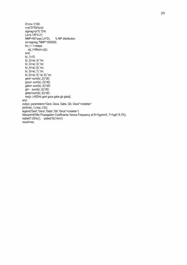
29
D=(nx-1)*dD; x=pi*D*fGHz/c0; sigmag=pi*D.*D/4; LA=4.1/R^0.21; NMP=N0*exp(-LA*D); % MP distribution sn=sigmag.*NMP*1000000; for j = 1:nsteps a(j,:)=Mie(m,x(j)); end; b(:,1)=D; b(:,2)=a(:,4).*sn; b(:,3)=a(:,5).*sn; b(:,4)=a(:,6).*sn; b(:,5)=a(:,7).*sn; b(:,6)=a(:,5).*a(:,8).*sn; gext= sum(b(:,2))*dD; gsca= sum(b(:,3))*dD; gabs= sum(b(:,4))*dD; gb= sum(b(:,5))*dD; gteta=sum(b(:,6))*dD; res(jr,:)=[fGHz gext gsca gabs gb gteta];end;output_parameters='Gext, Gsca, Gabs, Gb, Gsca*<costeta>'plot(res(:,1),res(:,2:6))legend('Gext','Gsca','Gabs','Gb','Gsca*<costeta>')title(sprintf('Mie Propagation Coefficients Versus Frequency at R=%gmm/h, T=%gK',R,TK))xlabel('f (GHz)'); ylabel('Gi(1/km)')result=res;