COMPUTATION OF STEADY AND UNSTEADY

QUASI--ONE--DIMENSIONAL VISCOUS/INVISCID INTERACTING

INTERNAL FLOWS AT SUBSONIC, TRANSONIC, AND SUPERSONIC

MACH NUMBERS

ir8

By

TIMOTHYW, SWAFFORD

DAVIDH. HUDDLESTON

JUDYA. BUSBYAND

B. LAWRENCECHESSER

NSF ENGINEERINGRESEARCHCENTERFOR COMPUTATIONALFIELDSIMULATIONMISSISSIPPISTATEUNIVERSITY

JUNE 1992

(.NASA-CP,-I_qOP1) C_MPUTATIr]N OF- STEADY AND

U_,t_TE _Y _dA S T-']_E:.-_ [ _EN.S I ONAL

VISCOU_/INVISCI n, INTERACIIN_ INTERNAL FLOWS

AT SU_.'_FINTC, TRANSONIC, AN_ SUPERSONIC MACH

NUMr';ER$ Final Report (MississiDpi State

NqZ-Z_55

UncI Js

MSSU-EIRS-ERC-92-1

https://ntrs.nasa.gov/search.jsp?R=19920019312 2020-04-30T14:15:05+00:00Z

COMPUTATION OF STEADY AND UNSTEADY

QUASI-ONE-DIMENSIONAL VISCOUS/INVISCID INTERACTING

INTERNAL FLOWS AT SUBSONIC, TRANSONIC,

AND SUPERSONIC MACH NUMBERS

by

Timothy W. SwaffordDavid H. Huddleston

Judy A. Busbyand

B. Lawrence Chesser

Engineering Research Center for Computational Field SimulationMississippi State University

FINAL REPORT

NASA LEWIS RESEARCH CENTERGRANT NO. NAG3-1170

June 1992

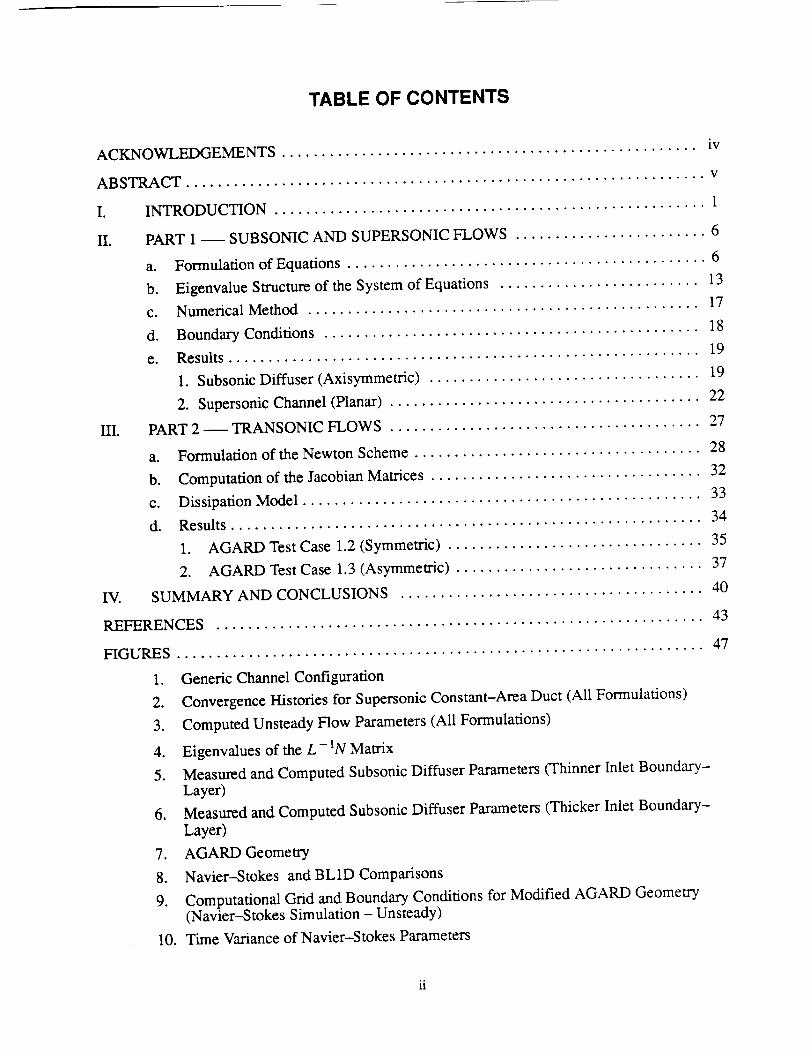
TABLE OF CONTENTS

ACKNOWLEDGEMENTS .................................................... iv

ABSTRACT ................................................................. v

I. INTRODUCTION ...................................................... 1

II. PART 1 _ SUBSONIC AND SUPERSONIC FLOWS ........................ 6

a. Formulation of Equations ............................................. 6

b. Eigenvalue Structure of the System of Equations ......................... 13

c. Numerical Method ................................................. 17

d. Boundary Conditions ............................................... 18

e. Results ........................................................... 19

1. Subsonic Diffuser (Axisymmetric) .................................. 19

2. Supersonic Channel (Planar) ....................................... 22

III. PART 2 -- TRANSONIC FLOWS ....................................... 27

a. Formulation of the Newton Scheme .................................... 28

b. Computation of the Jacobian Matrices .................................. 32

c. Dissipation Model .................................................. 33

d. Results ........................................................... 34

1. AGARD Test Case 1.2 (Symmetric) ................................ 35

2. AGARD Test Case 1.3 (Asymmetric) ............................... 37

IV. SUMMARY AND CONCLUSIONS ...................................... 40

REFERENCES ............................................................. 43

FIGURES .................................................................. 47

1. Generic Channel Configuration

2. Convergence Histories for Supersonic Constant-Area Duct (All Formulations)

3. Computed Unsteady Flow Parameters (All Formulations)

4. Eigenvalues of the L- 1N Matrix

5. Measured and Computed Subsonic Diffuser Parameters (Thinner Inlet Boundary-Layer)

6. Measured and Computed Subsonic Diffuser Parameters (Thicker Inlet Boundary-

Layer)

7. AGARD Geometry

8. Navier-Stokes and BLID Comparisons

9. Computational Grid and Boundary Conditions for Modified AGARD Geometry(Navier-Stokes Simulation - Unsteady)

10. Time Variance of Navier-Stokes Parameters

11. Navier-StokesandBL1D ChannelParametersat t _ 500

12. Navier-Stokes and BL1D Channel Parameters at t _ 1000

13. Navier-Stokes and BL1D Channel Parameters at t ---- 2000

14. Navier-Stokes and BL1D Channel Parameters at t ---- 3000

15. Momentum Thickness Distributions at t --- 1000 (Navier-Stokes)

16. AGARD Test Case 1.2

17. AGARD Test Case 1.3

APPENDIXES .............................................................. 89

I. Elements of the L and N Matrices ..................................... 89

II. Auxiliary Relations ................................................. 97

III. Details of Navier--Stokes Computational Procedure ....................... 98

NOMENCLATURE ......................................................... 100

iii

ACKNOWLEDGEMENTS

Research reported herein was supported in part by the NASA Lewis Research Center under Grant

NAG3-1170 with Dr. Jacques C. Richard as Technical Monitor, and also by the National Science

Foundation under the auspices of the Engineering Research Center for Computational Field Simula-

tion at Mississippi State University. This support is gratefully acknowledged. In addition, several

discussions with Dr. W. Roger Briley of the Engineering Research Center (ERC) for Computational

Field Simulation (CFS) concerning the ramifications of complex eigenvalues in relation to systems

of equations were extremely beneficial to this effort. Also, it was Dr. David L. Whitfield who sug-

gested trying the discretized-Newton scheme used in portions of this report, and many helpful

suggestions provided by him along the way added much needed interactions. This support is also

gratefully acknowledged. Finally, Mrs. Patty Pertuit had the patience of Job typing the manuscript,

and the authors appreciate her diligence and persistence.

iv

ABSTRACT

Computations of viscous-inviscid interacting internal flowfields are presented for steady and un-

steady quasi-one--dimensional (Q1D) test cases. The unsteady Q1D Euler equations are coupled

with integral boundary-layer equations for unsteady, two--dimensional (planar or axisymmetric),

turbulent flow over impermeable, adiabatic walls. The coupling methodology differs from that used

in most techniques reported previously in that the above mentioned equation sets are written as a

complete system and solved simultaneously; that is, the coupling is carried out directly through the

equations as opposed to coupling the solutions of the different equation sets. Solutions to the

coupled system of equations are obtained using both explicit and implicit numerical schemes for

steady subsonic, steady transonic, and both steady and unsteady supersonic internal flowfields.

Computed solutions are compared with measurements as well as Navier--Stokes and inverse bound-

ary-layer methods. An analysis of the eigenvalues of the coefficient matrix associated with the qua-

si-linear form of the coupled system of equations indicates the presence of complex eigenvalues for

certain flow conditions. It is concluded that although reasonable solutions can be obtained numeri-

cally, these complex eigenvalues contribute to the overall difficulty in obtaining numerical solutions

to the coupled system of equations.

I. INTRODUCTION

The study and analysis of internal flows has received significant attention over the past several de-

cades because the operation of many physical devices, particularly regarding aerospace-related

hardware, depend upon proper designs to achieve near-optimum operating characteristics. Exam-

ples of such devices include any configuration where the flow is confined and an exchange between

pressure and kinetic energy is desired (engine inlets, wind tunnel diffusers, rocket nozzles, etc.).

There devices can be geometrically complex as well as very viscous-flow dominated. Moreover,

certain configurations and conditions can result in unsteady flow (e.g., inlet buzz).

In the past, the design of these devices has, for the large part, depended upon empirically based meth-

odologies. More recently, computational techniques have played an increasingly important role in

the design process as hardware becomes less conservative and is required to operate "near the edge"

of the design envelop. As evidenced above, perhaps the most important physical flowfield charac-

teristics which need to be considered when attempting to computationally address internal flows are

effects associated with unsteadiness, viscosity, and multi-dimensions. Of course, the relative con-

tributions of these effects are dependent upon the geometry as well as which physical flowfield pa-

rameters are required to provide the "answers" for a given problem. For example, if the performance

(e.g., static pressure rise) of a subsonic axisymmetric diffuser is desired, it is very important that

viscous effects be well represented because diffuser performance is very sensitive, for example, to

the incoming blockage caused by the presence of the boundary layer. For this case, it can be argued

that unsteadiness and multidimensional effects play a secondary role. However, for cases where

boundary-layer separation is possible, significant unsteadiness may be present. For these cases the

capability to capture this unsteadiness within computation is important in order to gain engineering

insight into the physics. On the other hand, it is easy to identify cases where all of the above effects

play an important part in shaping the overall flowfield structure (e.g., a moving shock within an S-

shaped, asymmetric duct).

A thorough computational investigation of flowfields of this type requires solution of the full Re-

ynolds-averaged, multidimensional, time--dependent, Navier-Stokes equations. Of course, solu-

tionof theseequationsproducesessentiallyall pertinentflowfield parameters.Therefore,assuming

thatthesesolutionsareof acceptableaccuracy,it possibleto performparametricstudiesof apro-

posed geometry/flowfield combinationwhich could be used to significantly reduce the risk

associatedwith newhardwaredesign.Unfortunately,obtainingnumericalsolutionsto theseequa-

tionsfor complexgeometriesandunsteadyflowfields isexpensiveandtime--consuming,evenusing

today's largestand fastestsupercomputers.Therefore,it is importantto investigatealternative

meansof performingcompute-basedparametricstudiesof proposednew hardware designs. How-

ever, it is equally important that these alternative techniques be capable of capturing as much of the

critical physics as possible to avoid "throwing the baby out with the bath water." Consequently, iden-

tifying the physical aspects which tend to dominate the behavior of the flowfield associated with a

particular geometry is vital to the success of the alternative computational procedure.

It is obvious that some compromises must be made to reduce these computational requirements

while simultaneously retaining the desired physics. Deciding upon which compromise requires an-

swering the following question: "What are desired physics?" or stated another way, "Which physical

flowfield characteristics are we willing to approximate in order to reduce the overall computational

resource demands?" Unfortunately, the answer to either question is very problem dependent. For

example, elimination of viscosity effects from the Navier--Stokes equations results in the Euler

equations. Obviously, this reduced--equation set by itself can never be used to simulate the flow of

a viscous fluid, but can, however, be used to generate "reasonable" solutions for unsteady flow about

extremely complex, three--dimensional geometries, as demonstrated by Whitfield, et all who com-

puted the unsteady flow about three--dimensional transonic propfans using the Euler equations. The

precise meaning of "reasonable" relates to the above question(s). That is, an assumption was made

in Ref. 1, a priori, that viscous effects could be neglected for the configurations and flow conditions

to be investigated. Comparisons between measured and computed performance parameters 1 indi-

cated that this assumption was indeed "reasonably" valid. Therefore, it could be argued that the com-

promise made to exclude viscous effects from the analysis did not contaminate the computed solu-

tions to the point of being unusable. However, it should be pointed out that this conclusion is based

ontheoriginal stipulationthat(asanexample)effectsof viscosityandtheensuingramificationsof

its presencewereof lower priority in thesimulation.

Of thethreeaforementionedphysicalcharacteristicsunderconsideration,theonelikely to havethe

most significantimpactuponcomputationalresourcerequirementsconcernsthat of multidimen-

sions.Thiscanbearguedfrom thestandpointthatthenumberof floatingpoint operationsrequired

for agivensimulationis_ proportionalto (nna/'n)(2+ ndim) 2, where n is the number of grid

points and ndim is the number of spatial dimensions. Of course, this proportionality is greatly depen-

dent upon the numerical scheme used to solve the equations, but at least gives an indication of how

quickly the cost of performing multidimensional simulations escalates. Similar to the arguments

given above for three-dimensional viscous and inviscid flows, the validity of compromise (i.e., re-

duction) in the number of independent spatial variables is problem dependent and is difficult to

judge, a priori, whether the resulting simulation adequately represents reality. As stated by Hirsch 2,

"In all cases, however, the final word with regard to the validity of a given model is the comparison

with experimental data or with computations at a higher level of approximation." Therefore, it is

the reduction in effects associated with multi--dimensions, while retaining effects of unsteadiness

and viscosity, and solution of the resulting equations (for internal flows) which forms the basis and

underlying motivation of the present effort. In particular, the development of an engineering tool

through which preliminary estimates of unsteady internal flow processes can be generated using

available workstation-based hardware is sought.

One approach to achieve this is to seek solutions to the unsteady, two-dimensional Navier-Stokes

equations, or the unsteady two-dimensional Euler equations coupled with the steady (or unsteady),

two-dimensional boundary-layer equations. While these are valid approaches, even the two-di-

mensional equations can result in nontrivial computational time requirements, particularly for un-

steady flow. However, use of the coupling approach (e.g., Euler coupled with boundary layer) has

significant resource-saving advantages over that associated with solving the full Navier-Stokes

equations because of relaxed grid requirements in viscous regions 3. Hence, the coupling approach

is adopted here, where equation sets valid for a particular region of the flowfield are used. SpeciE-

cally,theEulerequationswrittenfor unsteady,quasi-one-dimensional(Q1D)flow arecoupledwith

integral boundary-layerequationsfor unsteady,two-dimensionalturbulent flow over adiabatic

walls. Theassumptionismadethatsolutionsto thecoupledequationswill yield resultsof engineer-

ingaccuracy.It mustbeemphasise&thatthevalidity of usingthesimplifiedequationsis veryprob-

lemdependentand,similartootheranalyticalorcomputationaltechniques,requiresexperienceand

engineeringjudgementwith regardto whethertheapproachand/orcomputedsolutionsrepresent

reality. No attemptsaremadeatquantifying specificclassesof problemsfor which theapproach

presentedhereincanbe used. Attempts are made to quantify the validity of these assumptions (or

lack thereof) through comparisons with available experimental and computational sources.

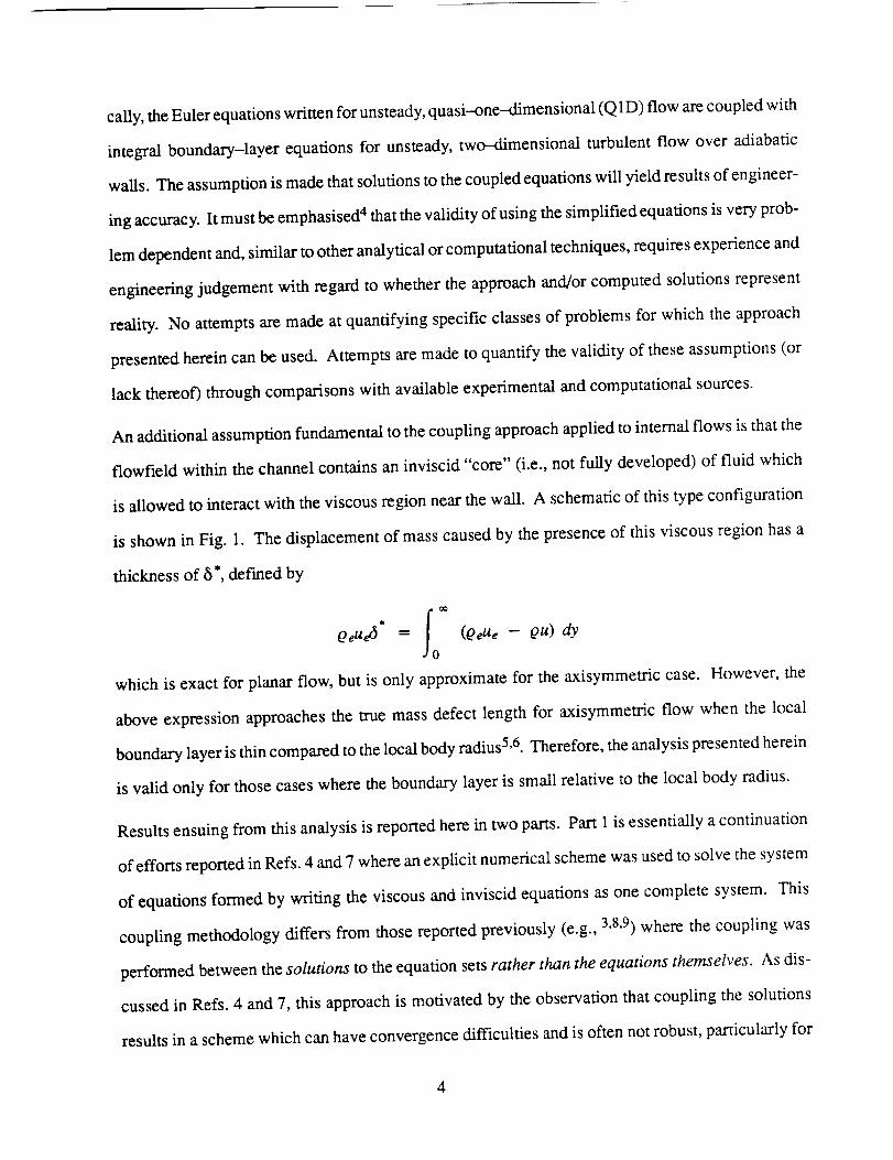
An additional assumption fundamental to the coupling approach applied to internal flows is that the

flowfield within the channel contains an inviscid "core" (i.e., not fully developed) of fluid which

is allowed to interact with the viscous region near the wall. A schematic of this type configuration

is shown in Fig. 1. The displacement of mass caused by the presence of this viscous region has a

thickness of 6", defined by

. I0°QeUet_ --- (OeUe - Ou) dy

which is exact for planar flow, but is only approximate for the axisymmetric case. However, the

above expression approaches the true mass defect length for axisymmetric flow when the local

boundary layer is thin compared to the local body radius 5,6. Therefore, the analysis presented herein

is valid only for those cases where the boundary layer is small relative to the local body radius.

Results ensuing from this analysis is reported here in two parts. Part 1 is essentially a continuation

of efforts reported in Refs. 4 and 7 where an explicit numerical scheme was used to solve the system

of equations formed by writing the viscous and inviscid equations as one complete system. This

coupling methodology differs from those reported previously (e.g., 3,8,9) where the coupling was

performed between the solutions to the equation sets rather than the equations themselves. As dis-

cussed in Refs. 4 and 7, this approach is motivated by the observation that coupling the solutions

results in a scheme which can have convergence difficulties and is often not robust, particularly for

4

"strong"interactioncases.In addition,previouscouplingschemeswhichusethesteady,directform

of theboundary-layerequationsto solvefor theviscousregionfor caseswhereboundary-layersep-

arationoccursfail becausethis form of theboundary-layerequationsaresingularator nearsepara-

tion3. (It shouldbenotedthoughthatthesingularitycanbeavoidedby usingtheso-calledinverse

form of the equations3. However,becausethe formulationof the unsteadyinverseform is not

unique,couplingof theviscousandinviscidequationsetsislessthanstraight-forward1°).Asshown

by Moses,et a111,however,asimultaneoussolutionprocedure(usingthesteadyformof thelaminar

boundary-layerequationsandLaplaceequationfor the streamfunction)apparentlyremovesthe

separationsingularitywhich makesthecomputationof separatedflows possibleusingthe direct

form of theboundary-layerequations.In ananalogousmanner,thepresentapproachsimultaneous-

ly solvestheunsteadyformsof theQ1DEulerequationsandtheunsteadyintegralboundary-layer

equationsfor turbulentflow for steadysubsonic(bothseparatedandattached)flows, aswell asun-

steadysupersonic(attached)flow cases.However,asdiscussedin subsequentsections,severalof

thedisadvantageswhich thepresentdirect couplingapproachsoughtto overcomehavebeenre-

placedwith other,perhapsmoredishearteningoneswith regardto seekingnumericalsolutionsof

thecompletesystemof equations.

5

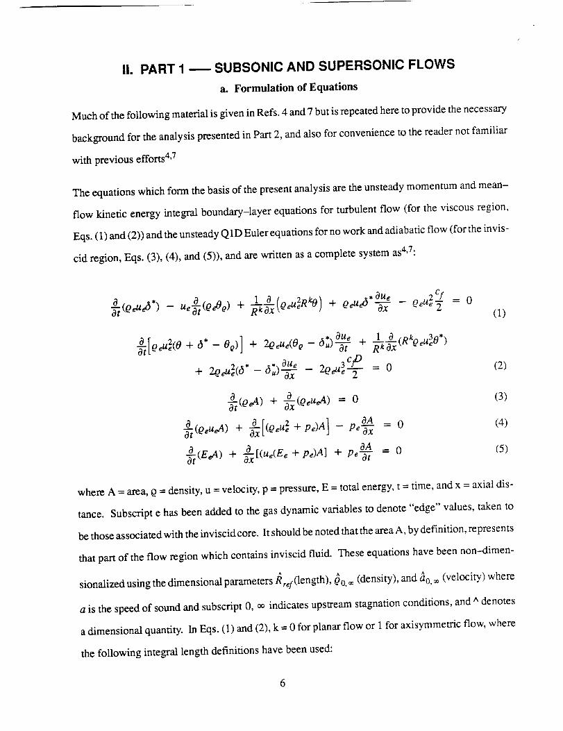
II. PART 1 _ SUBSONIC AND SUPERSONIC FLOWS

a. Formulation of Equations

Much of the following material is given in Refs. 4 and 7 but is repeated here to provide the necessary

background for the analysis presented in Part 2, and also for convenience to the reader not familiar

with previous efforts 4,7

The equations which form the basis of the present analysis are the unsteady momentum and mean-

flow kinetic energy integral boundary-layer equations for turbulent flow (for the viscous region,

Eqs. (1) and (2)) and the unsteady Q1D Euler equations for no work and adiabatic flow (for the invis-

cid region, Eqs. (3), (4), and (5)), and are written as a complete system as4,7:

a • ueO(o_e) + 1 a _ uZRhg_ .aue ,, ,2cf"_(QeUe_ ) - -'_-_Qe e ) 4" QeUe(} Ox _e,_e-_ = 0(I)

a 2 i_*-oQ)] .-1- 2_e/Je(0Q- ,.-,u/-_" -4- _--_-_+ o., : o (R%,3e05

2 * ,_*, aUe c_2+ 2QeUe((_ -_uJ "_ 2Qe u3 - - 0 (2)

0(004) +-b-x(e,u04) = 0 (3)

0 2 pc)A] Pe_xx - 0 (4)°(oeu04) + _[(eeu_ + -

-_(E04) + _x[(Ue(Ee + pc)A] + Pe_t t -- 0 (5)

where A = area, _ = density, u = velocity, p = pressure, E = total energy, t = time, and x = axial dis-

tance. Subscript e has been added to the gas dynamic variables to denote "edge" values, taken to

be those associated with the inviscid core. It should be noted that the area A, by definition, represents

that part of the flow region which contains inviscid fluid. These equations have been non-dimen-

sionalized using the dimensional parameters/_ref(length), _0. = (density), and a0, o_(velocity) where

a is the speed of sound and subscript 0, oe indicates upstream stagnation conditions, and ^ denotes

a dimensional quantity. In Eqs. (I) and (2), k = 0 for planar flow or 1 for axisymmetric flow, where

the following integral length definitions have been used:

6

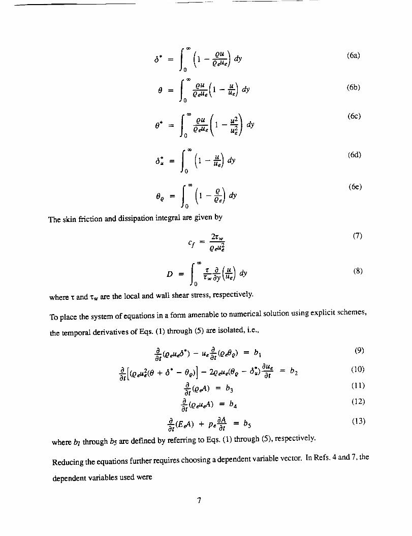
I0°( ),5* = 1 O0-_Ue' dy

o= 1-_

o0

" Io(u)6. = 1-_ dy

The skin friction and dissipation integral are given by

2_rwcl = 2--_..2

QeUe

(6a)

-°[(o;,,_(o+_"- oo)]-2o,uxOoOt

(QoA) = b 3

(OeueA) = b 4

_(EeA) + pe'_t t = b5

(6b)

(6c)

(6d)

(6e)

(7)

(8)

where x and xw are the local and wall shear stress, respectively.

To place the system of equations in a form amenable to numerical solution using explicit schemes,

the temporal derivatives of Eqs. (1) through (5) are isolated, i.e.,

a * _ u a(o_o) =_(Oeue6 ) _. b 1 (9)

- _,)-_[ = o2 (10)

(11)

(12)

(13)

where bl through b5 are def'med by referring to Eqs. (1) through (5), respectively.

Reducing the equations further requires choosing a dependent variable vector. In Refs. 4 and 7, the

dependent variables used were

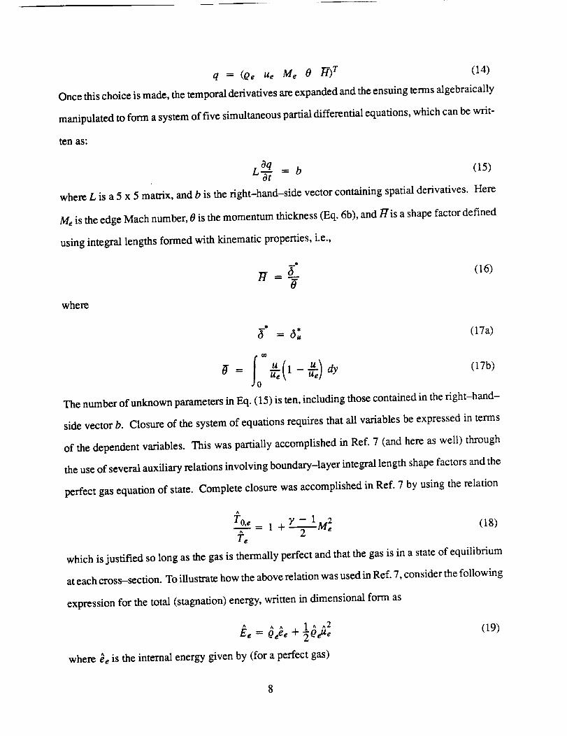
q = (Oe ue Me 0 T¥)T (14)

Once this choice is made, the temporal derivatives are expanded and the ensuing terms algebraically

manipulated to form a system of five simultaneous partial differential equations, which can be writ-

ten as:

3a

L_t = b (15)

where L is a 5 x 5 matrix, and b is the right-hand-side vector containing spatial derivatives. Here

Me is the edge Mach number, 0 is the momentum thickness (Eq. 6b), and His a shape factor defined

using integral lengths formed with kinematic properties, i.e.,

mill

_- = 6__ (16)

i

6-° = 6. (17a)

/0"( )Ul_U dy

where

(17b)

The number of unknown parameters in Eq. (15) is ten, including those contained in the right-hand-

side vector b. Closure of the system of equations requires that all variables be expressed in terms

of the dependent variables. This was partially accomplished in Ref. 7 (and here as well) through

the use of several auxiliary relations involving boundary-layer integral length shape factors and the

perfect gas equation of state. Complete closure was accomplished in Ref. 7 by using the relation

A

To y - IMa'----Ae= 1 +X e (18)

Te

which is justified so long as the gas is thermally perfect and that the gas is in a state of equilibrium

at each cross--section. To illustrate how the above relation was used in Ref. 7, consider the following

expression for the total (stagnation) energy, written in dimensional form as

^ ^^ 1^^2Ee = 0eee + _Qeue (19)

where _e is the internal energy given by (for a perfect gas)

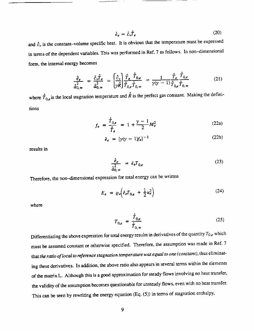
ee = cvTe (20)

and cv is the constant-volume specific heat. It is obvious that the temperature must be expressed

in terms of the dependent variables. This was performed in Ref. 7 as follows. In non-dimensional

form, the internal energy becomes

I 1 A A A

A A T Ae, _vT", cv T, O,e 1 Te To,e

^2 ^2 [_'_j r" r'-- = 1)7_0,,_0,ao, ® ao. o0 To,e TO,® 7(7 - ®(21)

where To, , is the local stagnation temperature and R is the perfect gas constant. Making the defini-

tions

results in

^

fe = TO'" _--_-7-- =1+ M_

T.(22a)

_, = [y(_, - 1)f,] - 1 (22b)

^

ee^_ = _eTo, ,

a0,_

Therefore, the non--dimensional expression for total energy can be written

where

(23)

(24)

^

To,eT0,, = 7--- (25)

T0,_

Differentiating the above expression for total energy results in derivatives of the quantity TO,e which

must be assumed constant or otherwise specified. Therefore, the assumption was made in Ref. 7

that the ratio of local to reference stagnation temperature was equal to one (constant), thus eliminat-

ing these derivatives. In addition, the above ratio also appears in several terms within the elements

of the matrix L. Although this is a good approximation for steady flows involving no heat transfer,

the validity of the assumption becomes questionable for unsteady flows, even with no heat transfer.

This can be seen by rewriting the energy equation (Eq. (5)) in terms of stagnation enthalpy,

9

where he is the stagnation enthalpy defined by

-- A_te (26)

h0

Use of the continuity equation results in

1 2

= he + _Ue (27)

Oho Oho I dpe (28)O---i"+ ue-_ = Qe Ot

We can rewrite the left-hand-side of the above as a material derivative to finally arrive at

Dh.._..oo .1 dpe= (29)Dt Oe Ot

which is valid in the absence of work and heat flux. By using the energy equation in this form, it

is straight-forward to see that changes in static pressure due to unsteadiness results in corresponding

changes in the stagnation enthalpy, and thus the stagnation temperature.

This situation can be avoided in at least two ways. One method is to express the internal energy

instead as

where

^ ^ ^

ee Cv Te Te

^2 " ^ 70,- 1)ao, ® yR To, ®

(30)

From the definition of the sonic velocity

^

TeTe ='7""--

To,®

(31)

^2 ^

ae ^Tea_ = ^-"i--= -- = T,ao,_ To,®

and using the Mach number, it follows that

(32)

which is the desired result.

^

eem

^2a0,_

y(y- 1)Me2 (33)

10

Another way to avoid making the constant stagnation temperature assumption is to replace Mach

number with static pressure as a dependent variable. To illustrate this, consider the perfect gas equa-

tion of state given by

or, in non-dimensional form,

Therefore,

^ A A

_, = OeRTe (34a1

OeTePe = -'7- (34b)

_Pg

7",=0--- 7

It follows that the Mach number can be computed as

A

Me -" UeUe

(Te) 1/2

(34c)

(35)ae

which again permits closure of the system.

Results ensuing from numerical schemes based upon allthree formulations are presented in this re-

port. As discussed in subsequent sections, both explicit and implicit numerical methods have been

implemented. Whereas an explicit scheme has been utilized in all formulations, the implicit method

has been applied to only the formulation where pressure is used as a dependent variable.

Because of the possible ramifications regarding solutions computed using the original formulation

which assumes constant stagnation temperature 7, a brief diversion will be taken at this point to inves-

tigate differences between computed steady and unsteady solutions resulting from the different for-

mulations. As mentioned above, numerical computations involving all formulations have been per-

formed using an explicit scheme (implementation of this scheme is discussed in Section II.c). To

investigate differences in computed solutions ensuing from these formulations, results for a constant

area axisymmetric duct (10 radii in length) with a fixed entrance Mach number of 2 and a reference

Reynolds number of 5 million are presented. Converged (steady-state) solutions from these com-

putations are shown in Figs. 2 and 3. Figure 2a presents time histories of exit Mach number and it

can be seen that identical results are obtained at steady state for all formulations. Also, convergence

11

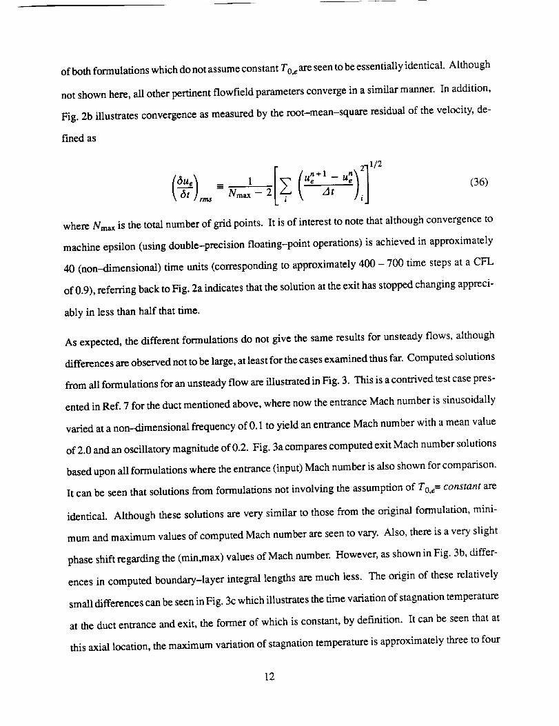
of bothformulationswhichdonotassumeconstantTo, eare seen to be essentially identical. Although

not shown here, all other pertinent flowfield parameters converge in a similar manner. In addition,

Fig. 2b illustrates convergence as measured by the root-mean-square residual of the velocity, de-

fined as

u. -[6ue_ 1 ° -At i (36)\_t]rms =-" Nrna_ - 2

where Nmax is the total number of grid points. It is of interest to note that although convergence to

machine epsilon (using double-precision floating-point operations) is achieved in approximately

40 (non-dimensional) time units (corresponding to approximately 400 - 700 time steps at a CFL

of 0.9), referring back to Fig. 2a indicates that the solution at the exit has stopped changing appreci-

ably in less than half that time.

As expected, the different formulations do not give the same results for unsteady flows, although

differences are observed not to be large, at least for the cases examined thus far. Computed solutions

from all formulations for an unsteady flow are iUustrated in Fig. 3. This is a contrived test case pres-

ented in Ref. 7 for the duct mentioned above, where now the entrance Mach number is sinusoidaUy

varied at a non--dimensional frequency of 0.1 to yield an entrance Mach number with a mean value

of 2.0 and an oscillatory magnitude of 0.2. Fig. 3a compares computed exit Mach number solutions

based upon all formulations where the entrance (input) Mach number is also shown for comparison.

It can be seen that solutions from formulations not involving the assumption of To,e = constant are

identical. Although these solutions are very similar to those from the original formulation, mini-

mum and maximum values of computed Mach number are seen to vary. Also, there is a very slight

phase shift regarding the (min,max) values of Mach number. However, as shown in Fig. 3b, differ-

ences in computed boundary-layer integral lengths are much less. The origin of these relatively

small differences can be seen in Fig. 3c which illustrates the time variation of stagnation temperature

at the duct entrance and exit, the former of which is constant, by definition. It can be seen that at

this axial location, the maximum variation of stagnation temperature is approximately three to four

12

percent.Therefore,anassumptionofTo,e= constant (used in the original formulation) is reasonable,

at least for this degree of unsteadiness.

Although differences exist between computed unsteady solutions that are based upon different for-

mulations of the system of equations, these differences are remarkably small, at least for the test case

shown. However, because the formulation which assumes To,e= constant is inconsistent with regard

to the simulation of unsteady flows, either of the new formulations are the preferred methodologies

in this regime. This is particularly true if the present coupling methodology is to be applied to cases

involving both unsteady flow and added heat flux.

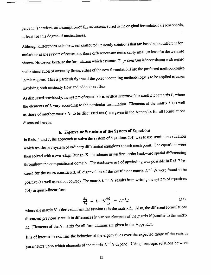
As discussed previously, the system of equations is written in terms of the coefficient matrix L, where

the elements of L vary according to the particular formulation. Elements of the matrix L (as well

as those of another matrix N, to be discussed next) are given in the Appendix for all formulations

discussed herein.

b. Eigenvalue Structure of the System of Equations

In Refs. 4 and 7, the approach to solve the system of equations (14) was to use semi-discretization

which results in a system of ordinary differential equations at each mesh point. The equations were

then solved with a two-stage Runge-Kutta scheme using f'trst-order backward spatial differencing

throughout the computational domain. The exclusive use of upwinding was possible in Ref. 7 be-

cause for the cases considered, all eigenvalues of the coefficient matrix L - 1 N were found to be

positive (as well as real, of course). The matrix L - 1 N results from writing the system of equations

(14) in quasi-linear form

aq L- 1NOq = L- ld (37)_ + ax

where the matrix N is derived in similar fashion as is the matrix L. Also, the different formulations

discussed previously result in differences in various elements of the matrix N (similar to the matrix

L). Elements of the N matrix for all formulations are given in the Appendix.

It is of interest to examine the behavior of the eigenvalues over the expected range of the various

parameters upon which elements of the matrix L- 1N depend. Using isentropic relations between

13

local staticandstagnationconditions,it is straight-forwardto showthat theseelements(andthus

theeigenvalues)canbeexpressedin termsof Me, H__and 0. Eigenvalue distributions as a function

of Mach number are shown (as lines) in Fig. 4 with both gand/9 used as parameters. The eigenva-

lues shown were computed using the elements of the L and N matrices resulting from the form ulation

where Me was used as a dependent variable but To, e was not assumed constant. (It is of interest to

note that eigenvalues computed using the formulation where Pe is a dependent variable are virtually

identical to those shown). Because of the algebraic complexity of the matrix L - 1N, the eignevalues

were computed numerically using an iterative technique 12. Also plotted in these figures (as sym-

bols) are the eigenvalues associated with the Q1D Euler equations written as an isolated system (Ue,

ue +a,, and ue - ae). It should be noted that Reynolds numbers were evaluated assuming reference

(stagnation) temperature and pressure to be 520°R and 14.7 psia, respectively. This results in mo-

mentum thickness Reynolds numbers ranging from approximately 400 to 480,000 for 0.001 < 0<0.1.

Figures 4a-4e (0"-0.001) illustrate eigenvalue behavior for 1.2 < H <__6.0. It can be seen that for

shape factors less than approximately 2.0, all eigenvalues remain positive for Mach numbers greater

than one thus confirming observations in Ref. 7. However, this is not the case for higher values of

H" as shown in Figs. 4d and 4e which indicate at least one eigenvalue becomes negative for Me >

1. Also, it is interesting to note that three eigenvalues of the complete system closely approximate

those of the inviscid equations for all values of/7.

Perhaps the most interesting (or disturbing) aspect of eigenvalue behavior can be seen in Figs. 4d

and 4e which indicate the appearance of complex conjugate pairs at high shape factors and superson-

ic Mach numbers, where the range of Mach numbers within which this occurs decreases with in-

creasing H'. While only the real part is plotted, the imaginary part is observed to be at least one order

of magnitude smaller than the real part. It should be noted that the appearance of complex eigenva-

lues seem to occur for shape factors high enough to be indicative of boundary-layer separation. Dis-

cussion regarding the ramifications of the appearance of complex eigenvalues is given at the end of

this section.

14

Onemighthopethatcomplexeigenvalueswouldoccuronlywithin arelativelysmallrangeof values

associatedwith thevariousparameters.Unfortunately,thisisnotthecasewhichis illustratedinFigs.

4f through40. InFigs.4f-4j (1.2_<H <-6.0,0=0.01), complexeigenvaluesagainappear,butonly

for shapefactorshigh enoughto causeboundary-layerseparation(which generallyoccursfor

2.8< H _< 3.0, depending upon the Reynolds number). The range of Mach numbers over which

this occurs is rather extensive at higher values of H. It should also be noted that significant deviation

from the inviscid eigenvalues has occurred at the higher values of momentum thickness, particularly

for higher shape factors. In addition, negative eigenvalues occur over the entire range of Mach num-

ber, again for higher values of H'. This behavior is even more pronounced for very high values of

momentum thickness as shown in Figs. 4k-4o (1.2 < H _<6.0, 0=0.1). However, one could argue

that for 0=0.1 we have violated one of the fundamental assumptions regarding use of the coupling

approach; i.e., recalling that 0 has been non--dimensionalized by a reference length (usually the inlet

radius or half-height), a value of 0=0.1 indicates that the local momentum thickness is 10% of the

local radius. Assuming a shape factor of 1.5 and that the local radius variation is small compared

to that of the inlet (which is consistent with the QID assumption) implies that the displacement thick-

ness occupies 15% of the channel radius. Assuming further that the displacement thickness is

approximately 1/6 of the total viscous region implies that the flow is essentially fully developed

which, of course, violates our original stipulation that this not be the case. Therefore, Figs. 4k--4o

should be interpreted as an illustration of how the eigenvalues behave toward the upper end of valid

parameter space. On the other hand, values of 0 in the range of 0.1 do not necessarily imply that

the channel is fully developed. For separated flows, integral lengths have the tendency to grow rap-

idly because of the large, retarded flow region near the wall. However, the overall viscous region

can remain small enough such that an inviscid core exits. Example of this are illustrated in subse-

quent sections.

The appearance of complex eigenvalues indicates that the system of equations in their present form

cannot allow solutions as a well-posed initial/boundary-value problem by integration over time.

This conclusion is based upon the work of Briley et all3 who used the criterion set forth by Garabe-

15

dian14"that it is naturalto requirethateveryroot of thecharacteristicequationbereal, asthisex-

cludessolutionsthatmaygrowexponentiallywith thetime-like variable"13.Therefore,exponential

growthin solutionsof a systemof equations(whichsupposedlyrepresentcertainphysics)canbe

attributedto numericalinstabilityof theunsteadysolutionalgorithmand/orto amathematicalset

of equationswhich is ill-posed for solutionsasaninitial valueproblemin time15.Differentiating

betweenthesetwoareasof concernfor thepresenteffort requiresthattheproblembeseparatedinto

itsindividualpieces,namely,physics,mathematics,andnumerics.Thatis,theobjectiveis to obtain

avalidmathematicalrepresentation(equations)of thephysicsandtonumericallysolvetheseequa-

tionsin a stablemannerto aspecifiedorderof accuracy.With regardto thephysicsof theinviscid

flow, it hasbeenwell establishedthattheEulerequationsrepresentavery goodapproximationto

themotionof afluid in regionswhereeffectsof viscosityareneglible. However,with regardto the

physicsof theboundary-layerflow,Whitfield 16encounteredcomplexeigenvaluesin seekingsolu-

tionstotheunsteadyintegralboundary-layerequationswheretimewasusedasaniterativeparame-

ter toreachsteadystate. In addition,similareigenvaluebehaviorwasencounteredin Refs.10and

17in dealingwith theunsteady,three--dimensionalintegralboundary-layerequationswhich,how-

ever,did not precludeobtainingreasonablenumericalsolutions10,17. Along these same lines, the

integral boundary-layer equations of the type used herein have been shown to yield good engineer-

ing approximations to viscous flows in regions where the usual boundary-layer assumptions are val-

id for both steady and unsteady regimes 6,18.

Based upon the above discussion, it is reasonable to conclude that it is the approximate governing

equations which are the origin of the observed anomalies. While the system of equations used in

the present effort does not generally exclude solutions exhibiting exponential growth due to ill-

posedness, it is shown in subsequent sections that numerical solutions of engineering accuracy can

be obtained for those cases where either: (a) no complex eigenvalues are encountered, or (b) if com-

plex eigenvalues do appear, unbounded growth can occur but can be very slow, thus allowing reason-

able solutions to be computed.

16

Becausethemethodpresentedhereinusesmanyof thesameshapefactorcorrelationsandauxiliary

relationsemployedin Refs.10and16,it isbelievedthattheappearanceof complexeigenvaluescan

beattributedto theapproximationsintroducedby these empirical and analytical relations; i.e., these

empirical relations and approximations are insufficient to define a well-posed set of approximate

governing equations. Of course, this situation calls for an analysis similar to that performed by

Briley 13 to attempt to locate the specific relations which cause the observed eigenvalue behavior.

Unfortunately, time and resource limitations preclude pursuing such an analysis.

c. Numerical Method

Based upon the preceding discussion, a numerical scheme utilizing spatial difference operators other

than purely one-sided is required for the general case unless, of course, a completely upwind method

which uses spatial differences whose type depends upon local flowfield characteristics (eigenvalues)

is used (note this approach is not even applicable for situations resulting in complex eigenvalues).

Because of the algebraic complexity of the governing system of equations and the above concerns

regarding well-posedness, an upwind approach was deemed inappropriate. Therefore, in the inter-

est of simplicity, the predictor-corrector MacCormack scheme 19 was utilized for the present effort.

MacCormack's scheme can be applied to a scalar (or system of) conservation law(s)

0__u + 2_ = 0 (38)at ox

. - a,vf,-- U i

.+1 = u7 + u g-- iU i

and is written as:

(39a)

(39b)

where subscript 'T' and superscript "n" denote spatial and temporal indices, respectively. Also, V

and A denote first-order backward and forward difference operators, respectively. In an analogous

manner, we can rewrite the present system of equations as

0__q+ b' = 0 (40a)Ot

where

17

b' = - L-lb

MacCormack's scheme is then implemented as:

(40b)

where, for example,

q_-TT = q7 + dtdq_ (41a)

q_+t _ l(qn + q_--4T) + ½ Atdqh_- _" (42)

dq n -= b 'n -. _ (L-lb) n (43)

In the predictor step, the vector function dq is evaluated using dependent variables computed at time

level n and inverting the matrix L at each mesh point. This inversion is carried out using an efficient

LU factorization 12. Spatial derivatives in the vector b are approximated (conservatively) using

first-order backward differences where variables are again evaluated at the nth time level. Similar

computations are performed during the corrector step, except that predicted values at time level

n + 1 are used to perform the matrix inversion, and first-order forward spatial differences are used

to approximate spatial derivatives. Because this is a central spatial difference scheme, additional

numerical dissipation must be added to suppress unwanted oscillations. A simple fourth--order mod-

el used by Warming and Beam 2° was used and implemented by modifying the corrector step Eq.

(32b) above to give:

where 2o

where CFL <_ 1 for stability.

number of 0.9.

qn+l _ l(qn + q_'r) + ½AtdqhjT + CsCo_d4qn (44a)i

64q_ = qni+2 - 4q_t+l + 6q7 - 4q7-1 + qn_2

c<o = 1 - CFL2

(44b)

(44c)

(44d)

All solutions computed with this scheme were obtained with a CFL

d. Boundary Conditions

For supersonic inflow and outflow, all dependent variables were specified and extrapolated, respec-

tively. Conditions at subsonic inflow and outflow boundaries were treated by considering the invis-

18

cidandviscousequationsseparately.Thatis,for subsonicoutflow,pressurewasspecifiedanddensi-

ty,velocity,andboundary-layerparameterswereextrapolated.Machnumberwasthendetermined

fromvelocity andthecomputedsonicspeed.Forsubsonicinflow, themethodproposedby Cooper

et a121wasusedfor theinviscidequations.By specifyinginflow stagnationconditions,thismethod

iteratively solvesfor thevariablesTe, Pc, and ue using the equations (non--dimensional)

7- 1 2 (45a)To, e = Te + 2 Ue

Te _ r'lv-1

Pe = PO, e\_o,e/

(45b)

P, (45c)C = Ue oeae

where Tis the temperature and a is the speed of sound. C used in Eq. (35c) is a"characteristic-like"

variable and is computed from information at the first mesh point inside the boundary 21. Boundary-

layer parameters 0 and ]7 are specified and held fixed at the inflow boundary.

e. Results

The objective of this section is to present comparisons between computations obtained using the

present interaction technique and measurements, as well as other computations. Subsonic and su-

personic results are reported in separate sections where subsonic comparisons are all for steady dif-

fuser flows, whereas supersonic computations are for both steady and unsteady channel flows. In

all computations shown here, 51 equally spaced points were used in the axial direction.

1. Subsonic Diffuser

Axisymmetxic subsonic diffuser flowfields investigated by Little et al22 are compared with those

computed using the present scheme (designated BL1D) in Figs. 5 and 6. The physical configuration

consisted of severalinlet pipe lengths (to give constant inlet boundary-layer thicknesses) and diffus-

er half-angles, although only comparisons for the 12 degree, 21 inch configuration for inlet bound-

,._* ._*

ary layer heights of 6 /Ri,an = 0.0034 (thinner inlet boundary layer) and 6 /Rinte t = 0.0190

(thicker inlet boundary layer) are reported here. It is almost embarrassing to report that computa-

19

tionsresultingfrom thepresentinteractionmethodrequiredup to 30,000timeiterationsto achieve

convergence.However,it wassuspectedbeforehandthatthiswouldbe thecaseusinganexplicit

numericalschemefor subsonicinternalflows. Becausetheinteractionmethodologywasof primary

interestfor thepresenteffort (in particular,obtainingconvergedsolutionswhich includedbound-

ary-layer separation),largeiterationcounts were considered an acceptable compromise between

simplicity and efficiency. No attempt was made to optimize the code which was executed on a Sili-

con Graphics, Inc. Personal IRIS 4d/30TG at a rate of 0.0016 cpu-seconds per time step per grid

point. Therefore, a test case with 51 grid points requiring 10,000 time iterations resulted in approxi-

mately 14 minutes of execution time.

Also shown for comparison are computed parameters using a more classical interaction technique

(herein designated as DUCFLO) where the inverse form of the steady integral boundary-layer equa-

tions are iterated with edge velocity obtained from the constant mass-flow constraint. The inverse

boundary-layer method used to obtain these results is that reported by Whitfield, et al23, although

the DUCFLO interaction code (written by Whitfield), and findings generated by this code, have not

been reported elsewhere. It should be noted further that this code can achieve converged solutions

much more quickly than that using BL1D. However, the DUCFLO formulation is valid only for

subsonic, steady flow and for this class of problems is generally the preferred technique with regard

to computational resource requirements.

Thinner Inlet Boundary Layer

Figs. 5a-5e present comparisons between measured and computed distributions of static pressure,

displacement thickness, momentum thickness, shape factor, and skin friction through the diffuser

for the thinner inlet boundary layer case (integral lengths were formed using only kinematic proper-

ties). Fig. 5a compares measured and computed static pressures (normalized by the inlet stagnation

value), where the exit pressure (in BL1D) was adjusted until that at the inlet station matched the mea-

sured value. Except for the region where diffuser diverence begins, computed pressures (from both

BLID and DUCFLO) are seen to compare favorably with those measured. It should be noted that

the computed inlet pressure using BL1D was somewhat sensitive to the specified exit pressure. That

2O

is,theexitpressureusedto obtainthedistributionshownin Fig. 5awasapproximately0.905,giving

in inletpressureof 0.60. Increasingtheexitpressureto approximately0.92resultedin aninlet pres-

sureof approximately0.66. Therefore,casesreportedin this section(usingBL1D) wereobtained

byadjustingtheexit pressureto matchthatatthe inlet.

Figs.5band5c comparemeasuredandcomputed"incompressible"displacementandmomentum

thicknessdistributionsthroughthediffuser. It canbeseenthatbothcomputationaltechniquesover-

predictandunderpredict_*and 0", respectively, although this agreement is considered reasonable.

As a result of this over- and underprediction, computed shape factors are correspondingly high, as

shown in Fig. 5d. It is reported in Ref. 22 that boundary-layer separation was not present in the

experiment and none is predicted by the computations. This is illustrated in Fig. 5e which presents

computed skin friction distributions (no measurements were available). However, exit shape factors

in the range shown in Fig. 5d are an indication that considerable retardation in the velocity profile

is present (i.e., the boundary layer is close to separation). This is illustrated in Fig. 5e which

compares measured and computed (from BL1D) velocity profiles at the diffuser exit, where mea-

sured profiles were obtained at three circumferential positions 1200 apart. Although agreement be-

tween measured and computed velocities is not particularly good at this axial location, considerable

scatter exists in the data. Nonetheless, the computed profile is too thin and is also more retarded near

the wall. However, as stated above, both measured and computed profiles are seen to be close to

separation.

Thicker Inlet Boundary Layer

Fig. 6 presents comparisons between distributions of measured and computed (BL1D and DUC-

FLO) diffuser parameters for the thicker inlet boundary-layer case. As stated previously, the exit

pressure was adjusted until the computed inlet pressure approximated the measured value. Similar

to the thinner inlet boundary-layer case, good agreement between measured and computed pressure

distributions is indicated in Fig. 6a, although there is a "kink" in that computed by DUCFLO. This

is apparently due to boundary-layer separation which is predicted by both BL1D and DUCFLO.

It can be seen in Fig. 6b that good agreement between measured and computed displacement thick-

21

nessis obtained(exceptnearthediffuserexit), althoughcomputedvaluesareagainslightly high.

Similar commentscanbemaderegardingmeasuredandcomputeddistributionsof momentum

thicknessshowninFig. 6c,althoughDUCFLOagainexhibitsamarked"kink" within theseparated

regionwhich is notevidentin theBL1D computation.As expected,computedshapefactorsare

againtoohighcorrespondingtooverpredicteddisplacementthickness.Theextentof boundary-lay-

er separationis showninFig. 6ewhichpresentscomputedskinfriction distributionsfor thethicker

inlet boundary-layercase. The DUCFLO computationsindicatea largerseparatedregion than

BL1D in thatseparationandreattachmentoccursfartherupstreamanddownstream,respectively,

thandoesBL1D (again,nomeasurementswereavailable).Figure6f givescomparisonsbetween

measuredandcomputedvelocity profilesatthediffuserexit. Again,measurementswereobtained

atthreecircumferentialpositionsaroundthediffuserexit. Thecomputedvelocityprofile showsno

reverseflow at thisaxial location(thecomputedboundarylayerhasreattached),whereasat least

onesetof thesemeasurementsindicatethattheflow is separated.However,theagreementbetween

measuredandcomputedvelocity profiles isconsideredreasonable.

2. SupersonicChannel

Steady and unsteady computations from BL1D for supersonic channel flows are compared to Navi-

er-Stokes calculations in this section. Although supersonic nozzle flow calculations were reported

previously 7, the test case reported in Ref. 7 was for steady flow and compared only measured and

computed wall static pressures. Attempts are made here to extend such comparisons to include the

boundary layer, particularly for unsteady flow.

Justification for comparing results ensuing from one computational technique to those of another

comes from Hi.rsh 2 in reference to comments made in the Introduction; that is, computations result-

ing from a Navier--Stokes analysis represent a higher level of approximation than those associated

with the present methodology. The supposition here is that the technique employing the higher level

of approximation is a better representation of the physics. While comparisons such as these are com-

mon within the technical community, favorable agreement does not necessarily mean that results

from the more approximate method represent reality; it just means that the two computations agree

22

with eachother. The pitfall here is that while techniques utilizing a higher degree of approximation

(i.e. more complete mathematics), may indeed represent more complete physics, the numerical

method used to solve the resulting equations may be such that these physics are masked or otherwise

lost. Therefore, in keeping with previous comments regarding distinctions between physics, mathe-

matics, and numerics, there can be no doubt that the Navier--Stokes equations are a more complete

mathematical representation of the physics associated with supersonic internal channel flows. How-

ever, we are assuming here that the numerical scheme used to give approximate solutions is yielding

these physics to an acceptable level of accuracy which, of course, results in a better representation

of the physics.

The Navier--Stokes method used to obtain viscous solutions presented herein is that developed by

Whitfield 2a and co--workers 25-26. The particular version used most closely resembles that reported

in Ref. 26 which has been modified to include explicit evaluation of viscous terms and extension

of the solution algorithm to the so--called "modified two-pass scheme". This code has as its basis

an Euler solver which is an implicit finite-volume, formulation applying Roe's 27 approximate Rie-

mann solver, and the higher--order extensions of Osher and Chakravarthy 28, to compute the inviscid

flux terms. The implicit operator is formed using Steger's 29 flux vector splitting with the resulting

system of equations inverted by application of Whitfield's 3° two-pass or modified two-pass algo-

rithm. The modified two-pass algorithm was applied in these computations. A brief description

of the numerical scheme is included in the Appendix and the reader is encouraged to seek out the

noted references for more details about the algorithm and the implementation.

Comparison between BL1D and Navier-Stokes computations were made for two test configura-

tions. The geometry analyzed was a transonic nozzle used as an AGARD 31 test case originally de-

signed for evaluation of Navier--Stokes simulation capability relative to shock/boundary-layer in-

teraction. To maintain isentropic, supersonic core flow, the nozzle pressure ratio was maintained

below the second critical design pressure for the present computations.

23

Comparisonsweremadeonthisgeometryfor twotestcases.Thefirst comparisonismadefor steady

supersonicflow subjectto fixed inlet totalpressureandtotal temperatureandprescribedexit static

pressure.Thesecondcaseis for anunsteadyflow andiscreatedbylinearlyincreasingtheinlet total

pressureasafunctionof time,whereasinlettotaltemperatureisheldconstantandexitstaticpressure

is againmaintainednearsecondcritical designpressure.Thegeometryis shownin Fig. 7a.

It shouldbepointedout thataproblemariseswhenmakingcomparisonsbetweentheQID analysis

andthetwo--dimensionalNavier--Stokesanalysis.In theQ1Dcomputationall flow-field parame-

tersataparticularinstantvaryonly asafunctionof axial location. However,eachNavier-Stokes

simulationproducesa two--dimensionalflow-field anddeterminationof equivalentone-dimen-

sionalflow parametersfor comparisonis atbestambiguous.Thisresultsfrom theobservationthat

determinationof theboundarylayeredgeis not uniquefor acomplexvelocity profile.

Steady Case

For Navier-Stokes analysis, the AGARD transonic nozzle 31 was modeled using 153 X 30 mesh

points in the axial and vertical directions, respectively. The grid spacing at the viscous wall, Ay/h

is approximately .0002 ( where h is the channel half-height). This corresponds to a y+ value of

approximately 4. The Reynolds number based upon reference conditions and channel half-height

is approximately 1.0 X 106. The grid used and the boundary conditions specified in this simulation

is shown in Fig. 7b.

Identical boundary conditions and nozzle area variation were used to preform a corresponding simu-

lation with the BL1D code beginning at axial location x=90mm, where inlet boundary conditions

were taken from the Navier---Stokes simulation. Comparisons of computed distributions of Mach

number, density, momentum thickness, and shape factor are shown in Figs. 8a-8d. Generally, agree-

ment between computed core parameters from the two methods is considered good. However, mo-

mentum thickness and shape factor do not agree as well, where the largest disagreement occurs for

150mm _< x < 250mm. Fig. 8e shows velocity profiles in the nozzle region which illustrates that

a unique definition of the boundary-layer edge is not possible thus causing the wide variations in

24

boundary-layerparameterscomputedfromtheNavier--Stokesresults.Thisillustrateshowthedefi-

nitionof quantitiessuchasmomentumthicknessandshapefactorlosetheir significancein thecon-

textof complexvelocityprofilessuchasthoseshownin Fig. 8e.

Unsteady Case

The AGARD nozzle geometry was modified for use as an unsteady test case. To produce a larger

region within which comparisons could be made, the nozzle geometry was arbitrarily extended (in

the axial direction) 4 nozzle heights as shown in Fig. 9. This geometry was then modeled with a

185 X 30 grid similar to the grid used for the steady test case (Fig. 7b). Boundary conditions were

as shown in Fig. 9. As stated previously, unsteady flow through the nozzle was initiated through

temporal variation of the reservoir total pressure, shown in Fig. 10a. A uniform time step was se-

lected such that the CFL number in the centerline region was near unity. This produced a maximum

CFL number in the viscous layer in excess of 103 . This is expected to adversely affect temporal accu-

racy of the simulation, but was deemed necessary in order to obtain results in a reasonable amount

of CPU time. The impact of high CFLs occurring within large regions of the viscous flow field was

not analyzed.

A portion of the nozzle geometry (shown in Fig. 9) was analyzed with BL1D for comparison pur-

poses. The Navier--Stokes simulation was used to define temporal boundary conditions at the inlet

of the "BL1D nozzle" (Fig. 9); these variations at x = 300 mm are shown in Fig. 10b. Comparisons

between computed distributions of Math number, density, momentum thickness, and shape factor

at non--dimensional times of approximately 500, 1000, 2000, and 3000 are shown in Figs. 11 through

14, respectively. At all time levels, agreement between computed inviscid core parameters (a and

b parts of Figs. 11 through 14) is considered very good. However, computed boundary-layer inte-

gral lengths do not agree nearly as well, although the overall qualitative trends of boundary-layer

behavior computed by BL1D are in good agreement with the Navier-Stokes results.

The reader should note the "waves" and "wiggles" in the Navier-Stokes results shown in these fig-

ures. As mentioned above, transforming two-dimensional results ensuing from the Navier--Stokes

25

analysishasprovedto besomewhatchallenging.Thesedifficultiescanbetracedfundamentallyto

one'sdefinitionof theboundary-layer"edge";i.e.,wheretheviscousregion"ends"andtheinviscid

core"begins". Integrallengthscomputedfrom theNavier-Stokessolutionpresentedhereinwere

generatedbystartingasearchatthewall for thef'trstmaximumvalueof velocity(ataparticularaxial

locationandinstantin time)whichwasthendefinedastheboundary-layeredge.Valuesof velocity,

density,andMachnumberatthisy-location werethenusedto generatethevariousintegrals.How-

ever,significantlydifferentvaluesof edgequantifiesareobtainedusinganotherdefinition. Forex-

ample,Fig. 15comparescomputedmomentumthicknessdistributionsfrom theNavier--Stokesre-

suits at the 1000time-level (this correspondsto Fig. 12d)using two different edgecondition

definitions.Fortheseconddefinition,thesearchdiscussedabovewasagainperformedtolocatethe

f'trstumax in a particular profile. This value of velocity was then multiplied by 0.99 and another

search conducted, again starting from the wall. The first index where the velocity exceeded the

0.99Umax value was then defined as the edge. This results in considerably different values of various

edge quantities, the result of which is illustrated in Fig. 15.

Therefore, although differences exist between computed unsteady core and boundary-layer quanti-

fies resulting from Navier-Stokes and BLID analyses, it appears that the Q1D approach is valid for

this type configuration, at least for the conditions investigated. Again, however, additional efforts

are warranted to investigate more consistent methods to interpret two-dimensional physics from a

one--dimensional perspective.

26

III. PART 2 _ TRANSONIC FLOWS

All previous discussion has been concerned with taking the system of equations (Eqs. (1) - (5)) and

algebraically manipulating various terms in order to recast the original system in a form amenable

for solution using relatively simple explicit numerical schemes. Although this approach has been

shown to be capable of quickly yielding solutions of reasonable accuracy (at least for the cases pres-

ented herein), the scheme possesses several distinct disadvantages. For example, many attempts to

compute solutions containing near--discontinuous behavior of the dependent variables (i.e., shocks)

with the explicit method have been unsuccessful, regardless of the type artificial dissipation model

used (including that used in the following implicit scheme-see Section III. c). Because the ability

to capture flows of this type is vital to any flow model which must operate in the transonic regime,

it was evident that another approach must be pursued.

Although not reported here, other explicit schemes have also been implemented, but again were not

capable of capturing solutions with steep gradients. Therefore, the decision was made to implement

an implicit scheme because of the inherent gains in stability bounds over those typically associated

with explicit methods. It should be noted that this decision was originally prompted by the issue

of numerical stability. It is recognized that if difficulties exist in obtaining numerical solutions for

an ill-posed initial/boundary-value problem, it is probable that one's choice of numerical scheme

is not relevant. As stated previously, the present system of equations exhibit complex eigenvalues

in flow regimes where shape factors (jr/') are high enough to induce boundary-layer separation.

However, the magnitudes of the imaginary part of these complex eigenvalues are observed to be very

small (one or two orders of magnitude less than the real part). One could interpret this as meaning

that the eigenvalue is "almost real" thus making the system "almost well-posed". Nonetheless, as

stated above, obtaining solutions using any scheme (especially those which are explicit) remains dif-

ficult and therefore we cannot discard the possibility that the system is fundamentally ill-posed in

certain flow regimes. Obviously, additional study is needed in this area.

The algebraic complexities of the present system of equations limit the number of implicit schemes

which can be used. For example, implicit schemes of Briley and McDonald 32 or Beam and Warm-

27

ing33cannotbeeasilyappliedtothissystembecauseit cannotbewrittenin fully conservativeform.

However,usingaNewton-basedimplicit solvercircumventsthislimitationbydiscretizingthesys-

tem in both time andspaceandtheniteratestheresultingsystemto convergence.The following

discussiondescribestheNewtonformulationaswell asotherissuesresultingfrom its use.

a. Formulation of the Newton Scheme

Following the analysis presented by Whitfield 3°, a classical implementation of Newton's method

for finding roots to a nonlinear scalar functionf(x) = 0 can be written as

f ,(x m) (xrn+ 1 _ x,n) = - f(x'n)

where m is an iteration parameter and

(46a)

dff' = (46b)

Now consider a system of nonlinear equations (each a function of several variables) written in very

general form as 29

(47)

Fn(xl,x 2, ...,Xn) = 0

If we consider F to be a vector function comprised ofF1, F2 ..... Fn, and x to be a vector function

comprised of xl, x2 ..... xn, then the above system of equations can be written simply as

F(x) -" 0 (48)

Newton's method for such a vector F(x) can be written analogous to that for a scalar equation and

solved as

x m+l = x m - [F '(xm)1-1 F(x m) (49)

In the above equation, F '(x) is the Jacobian matrix of the vector F(x) given by

28

F '(x)

al I (x)

a21(x)

a,,1(x)

a_2(x)

a22(x) a2,,(x)

a_2(x) ... a,,,,(x)

where the elements of the Jacobian matrix are given by

OFi(x)a_(x) = oxj

(50)

(51)

That is, the (ij) tlaelement of the Jacobian is given by the change in the ith element of the vector func-

tion F(x) for a given change in thej th dependent variable. Because it is usually impractical to obtain

the matrix inverse as the iteration proceeds, Newton's method is usually implemented as 30

F '(x'n)(x m+a - x m) = - F(x m) (52)

Now consider the vector function F(x) to instead be F(q), where the function F(q) is given by Eqs.

(1) - (5). For example, the first element ofF(q) is given by

O * ue 0 1 0 *F 1 = _(OeUe6 ) - _. (OeOo) + -_'-_ (Oeu2eR_) d- QeUe(_ OUeox ee,_e-_'_,2 cf = 0 (53)

In implementing the implicit scheme, the formulation involving pressure (Pc) as a dependent vari-

able was used. Thus, the dependent variable vector is given by

q=(o, u, p, 0 F1)r (54)

The remaining elements ofF(q) are defined by referring to Eqs. (2) - (5). The approach is to now

discretize these functions using first--order backward temporal differences (implicit Euler) and se-

cond--order central spatial differences, where the spatial differences are written at the (implicit) n+l

time level. This results in

29

F 1

F 2 =

o..n÷l _]Oeu,o )i - (Oeu_')

_7 - (u')7÷

+

i Xi+l -- Xi-1 J

" Cf" n+l

+ L x,_:,,j

(55)

[e,u_(0 + ,r - 0o)]_'+ 1 _ toque(0 + ,r - 0_)]7

(u,);'+1-(u,)_']At

_. ,,,÷_(u.)7++_ - (..)__:] "+:

n+l

+ _/_ x,+:- x-7:: j

=0 (56)

(O,a)7+: (O_)? .+l =+:- - (O_u,A)__:(O_u'A)i+iF3 = At + Xi+l -- Xi-I

=0 (57)

F 4 -

_n+ 1 an+ 1

(OeU,_4)7 + 1 [(O eu2 + P e)A ]i + 1 - [(Q eU2e+ p e)A li- 1+

At Xi+l -- xi-1

- --.(°_+: = 0Xi + 1 Xi - 1

(58)

F5 = (EeA)7+ lAt-(E_'4)n+ (Pe)in+Ir(A)_+I[At- (A)n]

[ue(Ee + n + 1 n + 1pe)A]i+ 1 - [Ue(Ee + pe)A]i_ 1= 0 (59)

+ Xi+ 1 -- Xi_ 1

Of course, we assume that variables at time level n are known and we seek to solve for those at time

level n+l. Therefore, within the framework of a Newton iteration, variables at the n time level are

constant. However, each function F(q) above depends upon values of the dependent variable vector

at spatial grid points i, i+l, i-l, all at the n+l time level. Thus, we can write

30

F(qn+1) = F:_n+1 n-l-l :_n+1'__c/i-!' qi _ti+I/

A Taylor's series expansion of F (qn+l) in three variables results in the expression

or

Fr-n+l +A-n+1 qn+l q_+1, qn+ll_'qi+l "'qi+l' " + A ._ + AqT_+:)

rll

_--n+1"m qn+l'm, _n+1"m)+ ( aF _ zlqn+l.m-" Pl'qi+l ' " qi-1 _1 i+1Oqi+l /

??It

+ Oqi_n+_ll Aqi-1

'" 7(aqF+Aq+ c) 1

where

m

_1 _ _ n+l'mcgqi+ 1

+

m m

OF Aqn+l'm + ' _n+l /Aqi-1Oqy+ 1 " aq i- 1

-n+ I,m An+ l'm, ..,n+ I,m)= -- F(qi+l 'qi tti-1

Aqn+l,m =_. qn+l,m+l _ qn+l,m

(60)

+l,m

(61)

(62)

(63)

Of course, the objective here is to perform sufficient iterations within a given time step such that

which gives

Aq n+ l"m _ 0 (64a)

qn+l,m+l _ qn+l,m = qn+l (64b)

Eq. (62) is the Newton scheme used herein. It should perhaps be referred to as a discretized-Newton

scheme because it is the discretized form of the equations to which the method is applied. The equa-

tion is written at each interior mesh point which results in a system of block tridiagonal equations,

where each block is a 5x5 matrix. A block tridiagonal solver written by Whitfield 16 is used to solve

the system of equations.

One should note that forming central differences on a non-uniform grid without the benefit of a cur-

vilinear coordinate transformation has altered the formal second--order accuracy of the spatial

discretization. This can be illustrated by considering a continuous functionf(x) defined at discrete

points xi and forming Taylor expansions for f(Xi+l ) and f(xi-I ) about f(xi), or

31

fi-1 = fi-- (Xi -- Xi-1) "_ i la _'_X2] i

Subtracting the latter from the former results in

_ , --r x,---_i- _ xi ,., -x,_, ]/Tx:/,

or,xix ,xx+ Lx,+i = x-?_i , ff+T=_,--?j

For uniform spacing, the second term on the right-hand-side of the above vanishes and the usual

central difference expression results. However, as evidenced by Eqs. (55) - (59), the present scheme

simply uses the first term on the right-hand-side of the above and consequently incurs additional

discretization error resulting from the non-uniform grid spacing. Fortunately, this additional "non-

uniform spacing error" is typically smallest in regions where grid spacing is smallest, and larger else-

where (at least using the stretching function discussed in Section III.d). Thererfore, the overall addi-

tional error will be counter-acted by the second derivative term which will be small if grid points

having the largest spacing have been placed in regions where the function is not changing rapidly;

i.e., Of/Ox _-- O.

As mentioned above, only the interior points are updated using the Newton iteration. Boundary

points are updated in an explicit manner at the conclusion of each complete time step in a manner

appropriate with conditions at the boundary (i.e., subsonic inflow, supersonic outflow, etc.), as dis-

cussed in Section ll.d.

The overall block structure is due to the appearance of the Jacobian roan'ices. Because of the algebra-

ic complexity of the vector function F(q), the Jacobians are evaluated numerically. This procedure

is discussed in the following section.

32

b. Computation of the Jacobian Matrices

Consider the following evaluation of a Jacobian using the dependent variable vector at the ith mesh

point:

where

OF) O(F1,F2,F3,F4,F5)T"_ i = O(ql,q2,q3,q4,q5) T(65)

(ql, q2, q3, q4, qs) r = (Oe, ue, pe, 0, F/) r (66)

Therefore, we can write the (rs) th element of the Jacobian at the ith grid point (at the mth iterate) as

OF cgFr rt_ls, i+ I ' qs, i qs.i- 1 ) -- rt_ls, i+ I ' "Zs,i ' qs, i- 1 )

+' = 07.+' =-- i r$ -- $,t

(67)

The above relation states that at the ith axial location, the (rs) th element is computed by evaluating

the change in the r th component of F(q) due to a given change in the sth component of q, holding

qs,i+l, qs,i-1 at their current mth-iterate values.

The value of e used to compute the Jacobians as described above was approximately one-half of the

reliable digits associated with the machine on which the code is executed, as suggested by Whit-

field 34. All solutions using the discretized-Newton scheme presented in this section were obtained

on a Silicon Graphics, Inc. 4d/460 Power IRIS using double-precision floating-point operations.

Therefore, for the present effort, t _ 10-6

As might be anticipated, computation of the Jacobian matrices is rather expensive from an operation

count point-of-view, particularly when considering that they appear within the Newton iteration;

i.e., they should be recomputed at each m-iterate. However, it has been observed that convergence

is not degraded significantly if the Jacobian updates occur infrequently. In fact, solutions presented

here were obtained by updating the Jacobians about every five time-steps, where a time-step may

include several m-iterations. This method of Jacobian updating drastically reduces the overall com-

putational resource requirements. Note that this approximation only affects the convergence (i.e.,

to make Aq n+l_n _- 0) at a particular time step and has no effect upon the time accuracy of the

33

scheme.This is becausethefight-hand-sideof Eq. (62)isonly affected by the discretization error

associated with the temporal and spatial difference operators used in the original discretization pro-

cess (in this case, f'trst-order in time and second-order in space).

c. Dissipation Model

As stated above, second-order central differences were used for spatial discretization. As such, in-

sufficient numerical damping is present which results in significant under- and overshoots in re-

gions where the dependent variables exhibit near-discontinuous behavior (e.g., shocks). Therefore,

additional artificial dissipation was needed to suppress these unwanted oscillations.

Although several dissipation models have been tried (e.g., that used by Warming and Beam2°), the

model proposed by Davis 35 has been the only one which yields the desired results. This is a "TVD-

based" (total variation diminishing) model which determines the level of added dissipation using

local flowfield conditions. The development of this model was motivated by the need to improve

shock capturing capabilities of explicit schemes while preserving the simplicity of these methods.

Much improved solutions were reported by Davis 35 in solving the two-dimensional Euler equations,

and also by Causon 36 who used the model in three--dimensional inviscid flows, where the MacCor-

mack scheme was used in both studies 35,36.

For the present discretized-Newton scheme, the additional dissipation was added to the dependent

variable vector at the end of each Newton iteration (i.e., after each m-iterate). Although adding the

dissipation at various other stages was tried, it was determined that adding it after each Newton itera-

tion was the most robust and gave the overall best results. The model as implemented herein is given

by the following step-by-step procedure:

m

[q_+l.,n+l] _ r.,,a+l,m+l] + 6qais s (68)smoothed- ttt i unsmoothed

where

34

6qais, l)(qi+l -- qi ) -- (Gi-1 + Oi )(qi - qi-1)

G_: = G(r_) - I/2C(v)[1 - 0(r_)]

l"

C(v) =_ v(1 - v),v <_o. 5

( 0.25 ,v > 0.5

v = v i = (CFL)i

(CFL)i = I/l,i l{zlt]_,Axsi

+ <(q_+l-qn_)'(q'_-qi'n-l))r i ---

((q_n+l _ q_n), (qm+l _ q_n)>

= -<(q_n _ qim_l),(qr _ qim_l)>

(69)

0(r) = min[mod(2r, 1)] = max(0, min(2r, 1))

where ( a, b ) is a scalar product of a and b, and _. is the maximum local eigenvalue.

d. Results

This section presents comparisons between measured 31 and computed results for steady, transonic

converging--diverging planar channel flow for both symmetric and asymmetric configurations. In

addition to results obtained by the present discretized-Newton scheme (hereafter designated

BL1D-I), calculations ensuing from both Navier-Stokes (the same code previously discussed) and

a QID Euler solver 37 are compared with the measurements. Solutions obtained with the discre-

tized-Newton scheme were obtained using a Silicon Graphics, Inc. 4cl/460 Power IRIS. Again, few

attempts have been made to optimize the code for fast execution which proceeds at a rate of 0.018

cpu-sec per grid-point per time-step. Calculations from BL 1D-I were obtained from an impulsive

start by initializing the dependent variables to specified values and then marching in time to a steady-

state.

With regard to the comparisons which follow, the reader should note that:

35

1. x -- 0 refers to the beginning of the convergent section.

2. All lengths have been non--dimensionalized with ht, where ht = 0.1 meter

for Case 1.2 and h t = 0.096 meter for Case 1.3.

3. Static pressures are plotted as a ratio of local static to reference stagnation

pressure (where/90. ® = 96 kPA).

4. Velocities are non--dimensionalized by the quantity Ue,max, where

Ue,max=418 meters/second for Case 1.2 and Ue,max---403 meters/second forCase 1.3.

Case 12 (Symmetric)

A schematic of the experimental apparatus (which is symmetric) is shown in Fig. 16a. In attempting

to computationally simulate the flowfield within a given physical configuration, it is important that

all pertinent information about the experiment be given. Unfortunately, a complete description of

the test apparatus was not provided in Ref. 31. In particular, the length of the section between the

reservoir and the beginning of the converging section, as well as the distance between the diverging

section and second throat, were not specified. Therefore, certain lengths had to be estimated where

both estimated and actual values are shown in Fig. 16a. Inlet stagnation pressure and temperature

were specified as 190,®= 96 kPA and I"0,® = 300 K, respectively. These conditions resulted in a refer-

ence unit Reynolds number of 5.345 x 105 per meter. Also, the reference length was defined to be

A

Rref= 50 mm.

For the present computations, 51 axial points were used where the points were clustered in the region

of the shock. The clustering was accomplished using a hyperbolic tangent stretching function given

by

where

x'=l+tanh[6(_- I)]

tanh(6)

_._ x-1Nmax- 1

Here 6 is a scale factor that controls spacing and Nmax is the number of axial grid points. Use of

such a stretching function allows a significant reduction in the number of grid points while maintain-

ing good resolution in regions of high gradients.

36

Comparisonsbetweenmeasuredandcomputedwall staticpressuredistributionsareshownin Fig.

16b. Symbolsrepresentmeasuredvalueswhereasthesolid line showsthecomputeddistribution

from theB11D-I code.Also shownfor comparisonis thecomputedpressuredistributionusingthe

inviscidmethodof Ref. 37. Bothmeasurementsandcalculationsindicatethepresenceof a shock

of moderatestrength.SimilartothesubsoniccalculationsdiscussedinSectionII, theexitstaticpres-

surein thecomputationswasadjustedin orderto matchthemeasurementsatsomeotheraxial loca-

tion. In thiscase,theexitpressurewassetsuchthatthecomputedshocklocationwasverynearthat

indicatedby theexperimentaldata. Althoughbothcomputationaltechniquesshowareluctanceto

expandasquickly asdo themeasurementsupstreamof theshock,theinviscidcalculationsshowa

muchhigherrateof compressionthroughanddownstreamof theshockthando thosecomputedby

the BL1D--I code. This "relaxing" effect is dueto thepresenceof the boundarylayer which, of

course,thepurely inviscidmethodcannotsimulate.

ShowninFig. 16cis thecomputedskinfrictiondistributionfor thiscase.Whereasnoexperimental-

ly determinedvaluesareavailablefor comparison,Navier-Stokesresultsareshownandareseen

to qualitativelyagreewith thosecomputedby BLID-I, althoughtheseparationpointsandthere-

gionsoverwhichseparationoccursareconsiderablydifferent. Notethatthecomputeddistributions

of cffrom both computational techniques are not smooth. In BL1D--I, this is due to similar behavior

of the calculated "incompressible" shape factor H, which is shown in Fig. 16d along with the mea-

sured distribution of this parameter. Although the computed distribution of Happears fairly smooth

in Fig. 16d, a scaled-up plot shows significant"wiggles" exist upstream of the shock (many attempts

to eliminate such oscillations have thus far been unsuccessful). The regions of experimentally and

computationally determined reverse flow are shown in Fig. 16d as the shaded and open areas, respec-

tively. Further illustrations of this reverse flow are given in Fig. 16e which show measured and com-

puted boundary-layer velocity profiles upstream and within the separated region, as well as at reat-

tachment. Also shown for comparison are Navier--Stokes calculations for the same configuration.

While the Navier-Stokes results show a clear superiority over those computed by BL 1D-I, the latter

technique is seen to capture the overall trends inferred by the measurements.

37

Finally,Fig. 16fpresentsacomparisonof measuredandcomputeddisplacementsurfaceswithin the

perspectiveof theexperimentaltestsection.It shouldbenotedthattheverticalandhorizontalscales

of this figurearedifferentwhichgivesadistortedview of theminimumarearegion. It canbeseen

that computedresultsindicatea displacementsurfaceconsiderablylargerthanthat measured,al-

thoughtheoverallqualitativetrendsassociatedwith rapid boundary-layergrowthdownstreamof

theshockarereasonable.Oneshouldnotethatthecomputeddisplacementthicknesswithin thesep-

aratedregiongrowsto approximately40%of thelocal channelhalf-heightwhich impliesthatthe

viscousregionoccupiesmostof thechannel(i.e., that theflow is fully developed).However,as

shownbythevelocityprofilesin Fig. 16e,therapidincreasein displacementthicknesscanbeattrib-

utedto thefactthatthevelocityratio U/Ue is highly retarded over a significant distance from the wall,

thus increasing the quantity 1-U/Ue used in computing the displacement thickness. Therefore, the

flow should not be considered fully developed and that an inviscid core does exist (which can be

verified from the velocity profiles shown in Fig. 16e).

Case 1.3 (Asymmetric)

The physical configuration for this case is similar to that given above except that the channel is now

non-symmetric. Again, a complete description of the test apparatus was not provided, thus making

it necessary to estimate the distance from the upstream reservoir to test section entrance. The exper-

imental apparatus is presented in Fig. 17a which shows an airfoil-like blockage, but is on the lower

wall only. Also shown in this figure is the computational domain used for the present calculations.

In reality, this is a two--dimensional configuration which, of course, cannot be completely simulated

using the Q1D approximation. However, because a large portion of internal flow configurations

possess some asymmetries, it is of interest to compare results from non-symmetric measurements

with those generated using the Q1D approximation in order to provide some measure of the validity

with regard to using the Q1D approach, particularly for transonic flow.

Shown in Fig. 17b are the actual and equivalent nozzle contours. The equivalent contour was gener-

ated by using the actual area and deducing from this the required channel half-height distribution.

38

It canbeseenthattheeffectof this"transformation"hasbeentolessenthewallslopesover the entire

airfoil region, particularly at the aft end where the airfoil and tunnel wall coincide.

Illustrated in Fig. 17c are comparisons between measured and computed static pressures where the

experimental data shown were obtained on the lower wall (refer to Fig. 17a) whereas those computed

result from use of the equivalent channel as discussed above (Navier--Stokes results were not avail-

able for this case). Also shown for comparison are wall pressures computed using the inviscid equa-

tions 37. Similar to the symmetric case, both computational schemes produce reasonable results up-

stream of the shock, and again the inviscid computations indicate a more rapid compression

downstream of the shock than do those associated with the present interaction scheme. Computed

pressures from the present scheme again exhibit "wiggles", but the oscillations seem to diminish

axially downstream. It is important to note that the exit pressure for both inviscid and interaction

calculations were adjusted such that the computed shock location approximated that observed on

the lower wall. For both calculations, the use of an equivalent area distribution has the effect of un-

der--expanding the flow in the region upstream of the shock. This is not surprising because the mea-

sured flowfield "sees" a larger disturbance on the lower wall than that within the equivalent channel.

Two--dimensional effects are shown in Fig. 17d which illustrates measured and computed pressures

for both upper and lower walls. It can be seen that significant differences exist between measured

upper and lower wall pressures and that the present calculations tend to represent an average of those

measured, except with regard to shock location. This figure further amplifies the previous observa-

tion that the equivalent channel (QID) approximation has the effect of causing a weaker shock (at

approximately the same axial location as that observed on the lower wall).

Similar to Case 1.2, a large region of separated flow was measured which is also predicted by the

computations. Figure 17e shows computed skin friction which illustrates the region over which

boundary-layer separation occurs in the calculations. The severity of the measured separation re-

gion is further illustrated in Fig. 17f which presents measured and computed shape factor (/-/) dis-

tributions. It can be seen that the calculated values of this parameter fall short of those measured

39

within theseparatedregion. Thereasonfor thisunderpredictionis shownin Fig. 17gwhich illus-

tratesmeasuredandcomputedvelocityprofilesasselectedlocationsin thevicinity of theseparated

region. It canbeseenthatreverseflow regionsassociatedwithcomputedprofilesarenotassevere

asthosemeasured,thusaccountingfor thelargeshapefactor. In addition,acorrespondinglylarge

displacementsurfacecomparedto thecomplicationsis shownin Fig. 17h. Whereasthecomputed

displacementsurfacedownstreamof theshockis lessthanthatmeasured,thecalculationsarecon-

sideredreasonable.This isparticularlytruewhenoneconsidersthelevelof approximationused in

the computational method. Similar to Case 1.2, this case does not appear to be fully developed thus

allowing the present interaction method to be applicable, at least for these flow conditions.

40

IV. SUMMARY AND CONCLUSIONS

Viscous-inviscid interacting internal flowfields have been computed for subsonic, transonic, and

supersonic quasi-one--dimensional (Q1D) configurations. Viscous-inviscid interaction was

achieved by directly coupling the unsteady Q 1D Euler equations with integral boundary-layer equa-

tions for unsteady, two--dimensional, turbulent flow over impermeable, adiabatic walls. The cou-

pling methodology differs from that used in the past in that the coupling is carried out directly

through the equations as opposed to solutions of the different equation sets. Numerical solutions

to the coupled system of equations were obtained using the explicit MacCormack scheme as well

as an implicit discretized-Newton scheme. Computed solutions have been compared with measure-

ments as well as Navier--Stokes and inverse boundary-layer methods. Although differences exist

between measurements and solutions computed from the QID approach, and also between those

computed by other methods, overall qualitative trends for both steady and unsteady test cases are

predicted with reasonable reliability.

An analysis of the eigenvalues of the coefficient matrix associated with the quasi-linear form of the

coupled system of equations used in the Q 1D approach indicates the presence of complex eigenva-

lues for certain flow conditions (in particular, values of shape factor, J_, high enough to cause bound-

ary-layer separation) thus allowing exponential growth in the solution(s). Although reasonable

solutions are obtained numerically, it is believed these complex eigenvalues contribute to the overall

difficulty observed in obtaining numerical solutions to the coupled system of equations. It is further

postulated that these complex eigenvalues are a result of empirical and analytical approximations

used in the integral boundary-layer technique.

The original formulation of the system of equations 7 (for use in the explicit scheme) made the as-

sumption that stagnation temperature was constant from the upstream xeservoir reference state to

that associated with local conditions. However, this assumption was shown to be inconsistent within

the context of unsteady flow, even for the case of no heat transfer. As a result, new formulations

of the equations were derived which do not depend upon an assumption of constant stagnation tem-

perature. It was shown that the degree of error associated with the original formulation was small,

41

atleastfor thecaseconsidered.However,thiserrorwill increaseindirectproportionwith thedegree

of unsteadinessassociatedwith aparticularflowfield.

ComparisonsbetweencomputationsusingtheQ1D approachandthoseresuhingfrom a Navier-

Stokesanalysisshowgenerallygoodagreementwith regardto theoverallqualitativeaspectsof the

flowfield. Someof theobserveddiscrepanciescanbeattributedto improperinterpretationof the

two--dimensionalNavier-Stokesresultsfrom theperspectiveof quasi--one-dimensionalphysics.

In particular,locatingtheboundary-layeredgeinaNavier--Stokesgeneratedvelocityprofileproved

to bethe"Achilles heal"of thecomparisonprocess.Nevertheless,resultsgeneratedfrom theQID

approachfor bothsteadyandunsteadysupersonicchannelflowsareconsideredgoodenoughto pro-

videpreliminaryestimatesof internalflowfield behavior,atleastfor configurationsof thetypecon-

sideredherein.

Implementationof animplicit discretized-Newtonschemefor numericallysolving the coupled sys-

tem of equations was originally motivated from the standpoint of numerical stability. This was

deemed necessary for the method to be capable of addressing transonic flow; i.e., flows with shocks.

However, as stated above, appearance of complex eigenvalues for the coupled system gives rise to

possible exponential solution growth due to the equations being ill-posed for solution in time as an

initial/boundary-value problem, at least in certain flow regimes. In spite of this, reasonable steady-

state solutions have been obtained, even for highly separated flows (i.e., for very high values of H).

It is concluded that even though the equations appear to be ill-posed in these regions, growth of error

is slow enough to allow reasonable solutions.

It is acknowledged that "there's nothing more dangerous than answers that look about right," and

that more study is warranted with regard to both unsteady and multi--dimensional flow, simulation

using the Q1D approach. However, it is felt that the Q1D approach is valid and the tools generated

by this effort are useful in the regimes which have been investigated, particularly when considering

the computational resources required to generate results from other methods. For example, the Nav-

ier-Stokes code used in these studies executes at approximately 6.0 x 10-5 cpu-sec per time-step

42

pergrid point ona CRAYY-MP. Therefore,for 3,000timestepsandthegrid used(185x 30x 2),

this resultedin approximately30cpuminuteson thismachine. As statedearlier,all Q1D-based

codeswereexecutedonengineeringworkstation-basedhardwareandrequiredmuchlesscomputa-

tional timetoexecute.Asstatedin theIntroduction,whetherornot theQ1Dapproachisappropriate

isgreatlyproblemdependent,asevidencedfromthesteady-statenozzleresultswhichwasinherent-

ly two-dimensionalwithin thenozzlecontraction/expansionregion. If preliminary,engineeringac-

curacyresultswill suffice,resultsshownhereinindicatethat thiscanbeachievedusingthisap-

proach.

43

REFERENCES

1Whitfield, D.L., Swafford, T.W., Janus, J.M., Mulac, R.A., and Belk, D.M., "Three-Dimensional

Unsteady Euler Solutions for Propfans and Counter-Rotating Propfans in Transonic Flow,"AIAA-87-1197, June 1987.

2Hirsch, C., Numerical Computation of Internal and External Flows, Volume 1: Fundamentalsof Numerical Discretization, John Wiley and Sons, New York, 1988.

3Whitfield, D.L., Swafford, T.W., and Jacocks, J.L., "Calculation of Turbulent Boundary Layerswith Separation and Viscous-inviscid Interaction," AIAA Journal, Vol. 19, No. 10, October 1981,pp. 1315-1322.

4Swafford, T.W., "Computation of Unsteady Supersonic Quasi--One-Dimensional Viscous-Invis-

cid Interacting Internal Flowfields," AIAA Journal, to be published.

5Cebeci, T. and Smith, A.M.O., Analysis of Turbulent Boundary Layers, Academic Press, New

York, 1974.

6Whitfield, D.L., "Integral Solution of Compressible Turbulent Boundary Layers Using ImprovedVelocity Profiles," AEDC-TR-78--42, Arnold AFB, TN, December 1978.

7Swafford, T.W., "Unsteady Viscous/inviscid Interaction via Direct Coupling of the ld-Euler and

2d-integral Boundary-Layer Equations," Mississippi State Engineering and Industrial ResearchStation Report MSSU-EIRS-ERC-90-1, March 1991.

8Carter, J.E., "A New Boundary-Layer Inviscid Interaction Technique for Separated Flow,"

AIAA-79-1450, July 1979.

9Kuhn, G.D., "Calculation of Separated Turbulent Flows on Axisymmetric Afterbodies IncludingExhaust Plume Effects," AIAA Journal, Vol. 18, March 1980, pp. 235-242.

l°Swafford, T.W., "Time-Dependent, Inverse Solution of Three-Dimensional, Compressible, Tur-bulent, Integral Boundary-Layer Equations in Nonorthogonal Curvilinear Coordinates," LectureNotes in Physics, Vol. 218, pp. 541-545, 1985.

11Moses, H.L., Jones III, R.R., and O'Brien Jr., W.E, "Simultaneous Solution of the Boundary Layerand Freestream with Separated Flow,"AIAA Journal, Vol. 16, No.I, January 1978, pp. 61--66.

12press, W.H., Flannery, B.P., Teukolsky, S.A., and Vettering, W.T., Numerical Recipes: The Art ofScientific Computing, Cambridge University Press, New York, pp. 365-376, 1986.

13Briley, W.R. and McDonald, H., "Three-Dimensional Viscous Flows with Large Secondary Ve-locity," Journal of Fluid Mechanics, Vol. 144, 1984, pp. 47-77.

lnGarabedian, P.R., Partial Differential Equations, John Wiley and Sons, 1964.

15Briley, W.R., Engineering Research Center for Computational Field Simulation, Mississippi StateUniversity, June 1992, Private Communication.

16Whitfield, D.L., Engineering Research Center for Computational Field Simulation, MississippiState University, June 1992, Private Communication.

17Swafford, T.W. and Whitfield, D.L., "Time-Dependent Solutions of Three-Dimensional Com-pressible Turbulent Integral Boundary-Layer Equations," AIAA Journal, Vol. 23, No. 7, pp.1005-1013, July 1985.

18Donegan, T.L., "Unsteady Viscous-Inviscid Interaction Procedures for Transonic Airfoil Flows,"MS Thesis, The University of Tennessee, Knoxville, TN, December 1983.

19MacCormack, R.W., "The Effect of Viscosity in Hypervelocity Impact Cratering,"AIAA-69-354, 1969.

2°Warming, R.F. and Beam, R.M., "Upwind Second-Order Difference Schemes and Applicationsin Aerodynamic Flows,"AIAA Journal, Vol. 14, No. 9, pp. 1241-1249, September 1976.

44

21Cooper,G.K. andSirbaugh,J.R.,"The PARCDistinction: A PracticalFlow Simulator,"AIAAPaperNo.90-2002.AIAA 27flaAIAA/SAE/ASME Joint Propulsion Conference, Orlando, Florida,1990.

22Little, B.H., Jr. and Wilbur, Stafford, W., "Performance and Boundary-Layer Data from 12 ° and

23 ° Conical Diffusers of Arca Ratio 2.0 at Mach Numbers Up To Choking and Reynolds NumberUp To 7.5 X 106, '' NACA Report 1201, 1954.

23Whiffield, D.L., Swafford, T.W., and Donegan, T.L., "An Inverse Integral Computational Methodfor Compressible Turbulent Boundary Layers," Recent Contributions to Fluid Mechanics, Editedby W. Haase, Springer-Verlag, 1982, pp. 294-302.

24Whitfield, D.L., Janus, J.M, and Simpson, L.B., "Implicit Finite Volume High Resolution Wave-

Split Scheme for Solving the Unsteady Three-Dimensional Euler and Navier-Stokes Equations onStationary or Dynamic Grids," Engineering and Industrial Research Station Report MSSU-EIRS-ASE-88-2, Mississippi State University, February 1988.

25Simpson, L. Bruce and Whitfield, David L., "Flux-Difference Split Algorithm for UnsteadyThin-Layer Navier-Stokes Solutions," AIAA Journal, Vol. 30, No. 4, April 1992, pp. 914-922.

26Arabshahi, A. and Whitfield, D.L., "A Multiblock Approach to Solving the Three-DimensionalUnsteady Euler Equations about a Wing-Pylon-Store Configuration," AIAA-89-3401-CP, June1989.

27Roe, EL., "Approximate Riemann Solvers, Parameter Vector, and Difference Schemes," Journal

of Computational Physics, Vol. 43, p. 357, 1981.

28Osher, S. and Chakravarthy, S., "Very High Order Accurate TVD Schemes," ICASE Report No.

84-44, Sept. 1984.

29Steger, J.L. and Warming, R.E, "Flux Vector Splitting of the Inviscid Gasdynamic Equations with

Applications to Finite Difference Methods," Journal of Computational Physics, Vol. 40, pp.263-293, 1981.

3°Whiffield, D.L., "Newton-Relaxation Schemes for Nonlinear Hyperbolic Systems," Engineeringand Industrial Research Station Report, Mississippi State University, No. MSSU-EIRS-ASE-90-3, October 1990.

31Advisory Group for Aerospace Research and Development (AGARD), Air Intakes for HighSpeed Vehicles, Section 3.3.1, Test Case 1, Transonic Normal Shock/Boundary Layer Interactions,AGARD Advisory Report 270, Fluid Dynamics Panel Working Group 13, September 1991.

32Briley ' W.R. and McDonald, H.,"S olutions of the Multidimensional Compre ssible Navier-S tokesEquations by a Generalized Implicit Method," Journal of Computational Physics, Vol. 24, pp.372-397, 1977.

33Beam, R.M. and Warming, R.E, "An Implicit Finite-Difference Algorithm for Hyperbolic Sys-tems in Conservation Law Form," Journal of Computational Physics, Vol. 22, pp. 87-110, 1976.

34Whiffield, David L. and Taylor, Lafe K., "Discretized Newton-Relaxation Solution of High Reso-

lution Flux-Difference Split Schemes," AIAA-91-1539-CE June 1991.

35Davis, Stephen E, "TVD Finite Difference Schemes and Artificial Viscosity," NASA-

CR-172373 (ICASE Report No. 84-20), June 1984.

36Causon, D.M., "A Total Variation Diminishing Scheme for Computational Aerodynamics," Nu-

merical Methods for Fluid Dynamics III, Edited by K.W. Morton and M.J. Baines, ClarendonPress, Oxford, pp. 449-457, 1988.

37Stokes, M.L., "A Solution of The Euler Equations on An Unstructured Grid System," PhD Dis-sertation, The University of Tennessee, Knoxville, Tennessee, May 1990.

38Baldwin, B.S. and Lomax, H., "Thin Layer Approximation and Algebraic Model for SeparatedTurbulent Flows," AIAA Paper No. 78 -257, AIAA 16 m Aerospace Sciences Meeting, Huntsville,Alabama, January 1978.

45

39Thomas,ED., "NumericalMethodfor PredictingFlow CharacteristicsandPerformanceof Non-axisymmetricNozzles-Theory,"LangleyResearchCenter,NASA CR 3147,September1979.

46

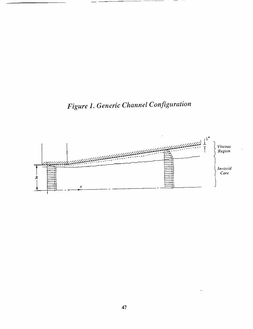
Figure 1. Generic Channel Configuration

R

L_

Viscous

Region

lnviscid

Core

47

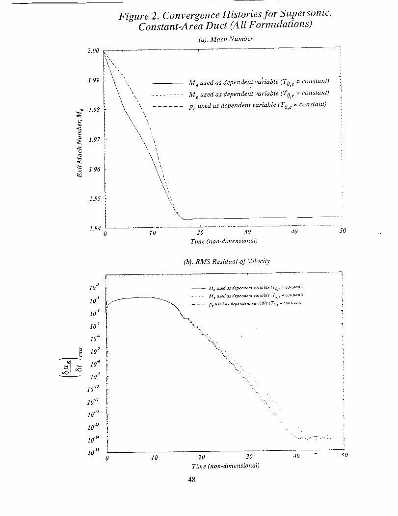
2.00

1.99

1.98

1.97 I

1.96

1.95

1.940

Figure 2. Convergence Histories )'or Supersonic,Constant-Area Duct (All Formulations)

(a). Mach Number

\

"\

\ \_, - ........

i J

10

M e used as dependent variable (To, e = constanO

M e used as dependent variable (To, e _ constant)

Pe used as dependent variable (To, e _ constant)

20 30

Time (non-dimensional)

40 50

(b). t_IS Residual of Veloci_

10 .2

10 _

10 -_

10 "s

10 .6

10 .7

10 -s

10 .9

10 -_o

10 "n

10 12

10 .23

10 "14

10 -_5

Y

\

-- M e used as dependent rarfable (To, e = co._tant)

Me used as dependent variable (To, e * cotlstattt)

-- -- -- Pe used as dependent variable ('I"0,e . cv._m,_t)

,\ \

!.

...... :-:---7--,. -.

10 20 30

Time (non-dimensional)

48

4O 5O

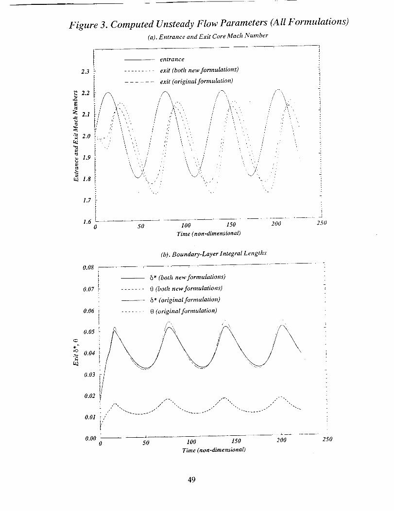
Figure 3. Computed Unsteady Flow Parameters (All Formulations)

(a). Entrance and Exit Core 31ach Number

2.3

entrance

......... exit (both new formulations)

2.1

_ 2"0 _'_ i _" J

° !_ 1.8 i

1.7 )

1.6 ! .....

exit (original formulation)

/ \t . .., '\..

• , f\',

1' _i

',' t t I '" /

i,

" \

"_-/ t,_ , \ , ,

//

' /

, /, /

t

/\ , t

\

\ ,-

r,' '_

0 50 100 150

Time (non-dimensional)

200

i

250

0.08

(b). Boundary-Layer Integral L engths

o_

0.07

0.06

0.05

0.04

0.03

0.02

0.01

0.00

6" (both new formulations)

....... e (both new fortnulations)

_* (original fornzulation)

_r ....... 0 (original formulation)

r t'_ I '\, ¢

t , , / ", / - ,

t-'

t,

0 50 I00 150 200

Time (non-dimensional)

250

49

1.15

0.95

F

0.90 i

I

0.85

0.80 _0

Figure 3. (Continued)

(c). Stagnation Temperature Variation

i 1

.... enlrance

exit

J

i

JIi

J

50100 150 200 250

Time (non-dimensional)

5O

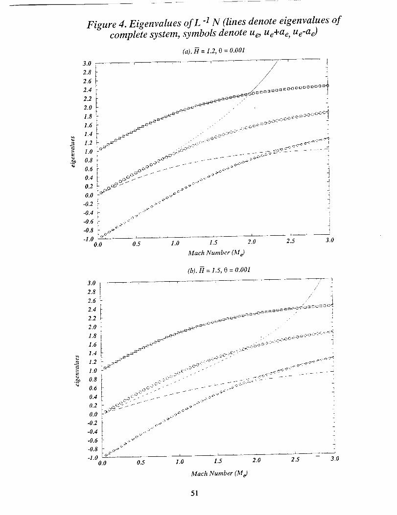
eo

3.0

2.8

2.6

2.4

2.2

2.0

1.8

1.6

1.4

1.2

1.0

0.8

0.6

0.4

0.2

0.0

.0.2

.0.4

-0.6

-0.8

-1.0

Figure 4. Eigenvalues of L -1N (lines denote eigenvalues of

complete system, symbols denote Ue, Ue+ae, Ue-a e)

(a). H = 1.2, 0 = 0.001

0.0 0.5 1.0 1.5 2.0 2.5 3.0

Mach Number (M e)

(b). It = 1.5, 0 = 0.001

2.6

2.4

2.2

2.0

1.8

1.6

1.4

1.2

1.o

0.8

0.6

0.4

0.2

0.o

.o.2

.o.4

-o.6

-0.8

-1.00.o

f /, __

; _0 _ _ _ ._ _ . .... -=

:L L," ""

I

0.5 1.0 1.5 2.0 2.5 3.0

Mach Number (M e)

51

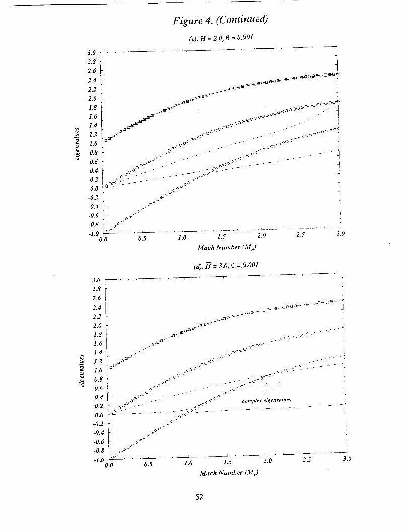
Figure 4. (Continued)

(c). H = 2.0, 0 = 0.001

Mach Number (Me)

(d). H = 3.0, O =.0.001

Mack Number (M e)

52

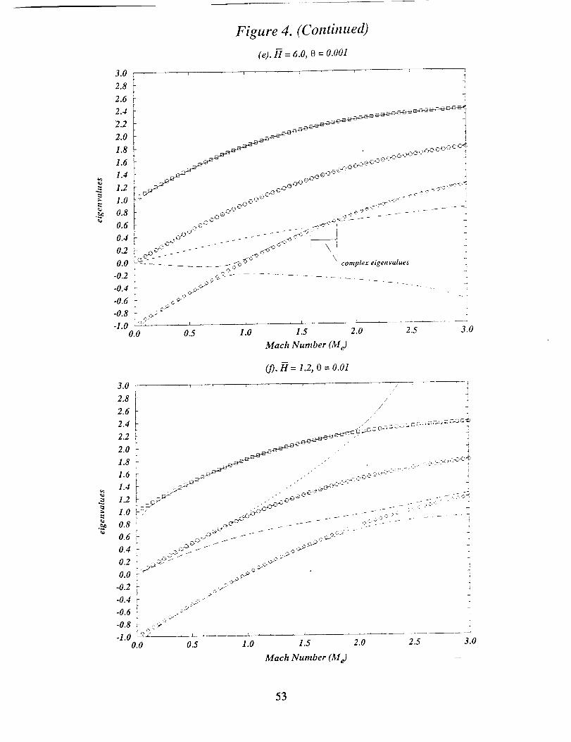
_o

Figure 4. (Continued)

(e). H = 6.0, t3 = 0.001

0.0

-0.2 _ 9 q "-- ......................

-0.4 ,.._._"

-0.6 _ _ _ _

-0.8 _ __.._"-I.0 _.,k' _ k k

0.0 0.5 1.0 1.5 2.0

<,<>v ""complex eigen values.q

2.5 3.0

Mach Number (Me)

09. H = 1.2, 0 = 0.01

eo

Mach Number Of e)

53

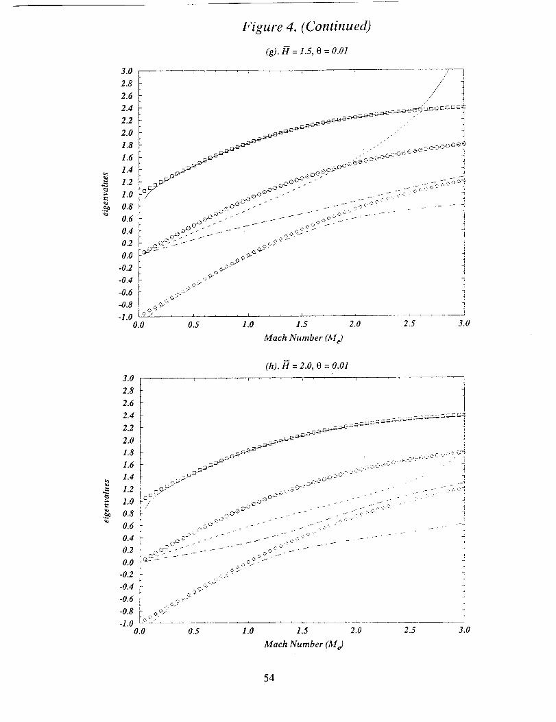
3.0

Figure 4. (Continued)

(g). B = 1.S, O = 0.01

/'

3.0

2.8

2.6

2.4

2.2

2.0

1.8

1.6

1.4

1.2

1.0

0.8

0.6

0.4

0.2

0.0

-0.2

-0.4

-0.6

-0.8

-1.0

I I

1.0 1.5 2.0 2.5 3.0

Mach Number (M e)

(h). _ = 2.0, 0 = 0.01

_ / 0.o Oz_

_Z- _ 0 0 " J" "0 I"

:z,

- .. ,?,.>

)<,o?S0.0 0.5 1.0 1.5 2.0

Mach Number (Me)

2,5 3.0

54

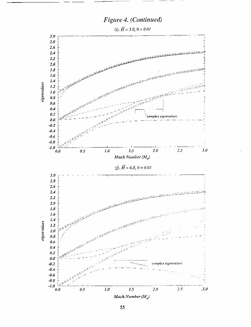
3.0

2.8

2.6

2.4

2.2

2.0

1.8

1.6

1.4

1.2

1.0

0.8

0.6

0.4

0.2

0.0

-0.2

-0.4

-0.6

-0.8

-1.0

Figure 4. (Continued)

(i). H = 3.0, o = o.ol

0.0 0.5 1.0 1.5 2.0 2.5 3.0

Mach Number (At e)

3.0

2.8

2.6

2.4

2.2

2.0

1.8

1.6

1.4

1.2

1.0

0.8

0.6

0.4

0.2

0.0

-0.2

-0.4

-0.6

-0.8

-I.0

(j). H= 6.0, 0 = 0.01

0.0 0.5 1.0 1.5 2.0 2.5 3.0

Mach Number (M e)

55

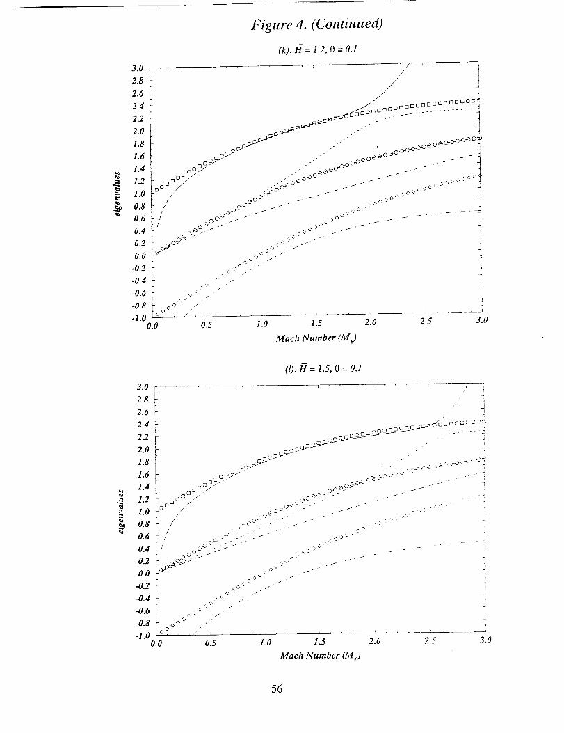
_o

_o

Figure 4. (Continued)

(_). _ = 1.2, o = o.i

3.0 .... ' ' /" !2.8 /

2.4 oczcz_aoaa_

1.8 eeC_oOc_e

1.6 __ eeee /_/_ _!,,4 o:::O0 .- - .'' _0 @

z _ / .-:_ ___ _ oo_.C,,-o _ :

0.8 _ / _z,':- _ _ _ oo c + _ ....0.6 _ / -_" I- _,o° .----- ,

0.4 _- _ oo -_

0.2 '- _ '0" _ ]

0.0 _ ,._e .- _-0.2 _- • ""

[ , o '_" / "

-0.4 '-- ..." .- _

-0.6 " .+,.'" •$- , -"

-0.8 _- <,oO" .. !-1.0 [_ " " +" " -_ , , i

2.0 2.5 3.00.0 0.5 1.0 1.5

Mach Number (M e)

3.0

(l). H =1.5, 0=0.1

e_

/ ;2.8 _ ....

2.6 i2.4 .... _:_"c _ c _:u c :_'_

2.2 [ ,,_ c_c _ . " "" _ ' !l1.8 L _-_'_ , ." :_.-_:,+:':<"'?

1.6 _ +=c:.%- ...._÷:_,>L_-- _ +-]

1.2 L _z / ....-c+G_.-" ..- ]

0.8 " _ _ " " ..... _ "

0.6 ?_ _ - _ ,o0.4 r/ .2-_ .-%- _ ..-: + ..... :

0-2 .+'+'+"+' ----t .._:- " ,.>>" +_

0.0 k :-"" ,,++' -_-_

-0.2 u _c." . 7

-0.4 _ ¢ <>" Ih ,:, '= . - / ]

-0.6 i ++.c'>'> "" "

-0.8 _ o" /-i.O I<>?°, :, , ........... .......

0.0 0.5 1.0 1.5 2.0 2.5 3.0

Mach Number (M e)

56

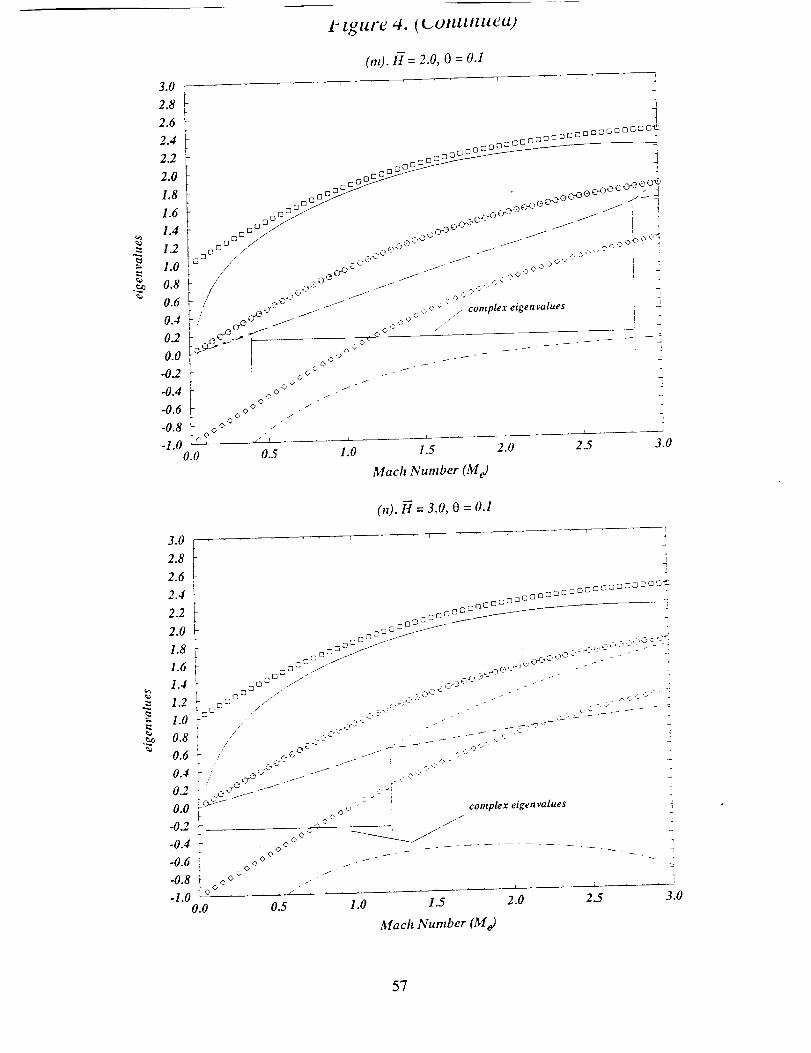
e_

1_ tgure 4. (contuulea)

010. H = 2.0, 0 = 0.13.0

2.8 _ jI

2.6 _ 42.4 !

2.2 _oa_ou_2 -- j2.0 o o o oS..Y-=-------_

1.8 ooo_

1.6 o °:z_'_'_ ' c_oe_eC_ee_>°eC _d1.4 _ _ n_ __._,o o'_ / , ,

= a'_-/ _:.eec-C ..... __ _J io ° t/ _,-_oc 'v'" - / I

1.2 -° a / _,-.o°'z°_ / / Lo<_

/ _£_'- / , _ ,.,c '_° - , .

0.8 _ /" £,_OOe O_ //_ / / ,^cooOCO ''_ !:0.6 , / ,_°_:_ / .. ,_c,'>'>" _ 5

0.4 [1 _ 0"_ / _ o+ ° c " / complex eigenvalues i ]

0.2 k ere,. _ + 0° /. i_-,z.9_ _ _ . r, o / r j

0.0 _ I +o",_o_ ................. i- -_

-0.4 _ o o _ _ . ---0.6 _ °°° "1 - _ " ]

^0 O0 / "" - -;

-0.8 b o °_ z +Lo? --1,0 / _ , , '-

- !

0.0 0.5 1.0 1.5 2.0 2.5 3.0

Mach Number (Me)

OO. H = 3.0, 0 = 0.1

complex eigen values

1.0 1.5

Mach Number (Me)

57

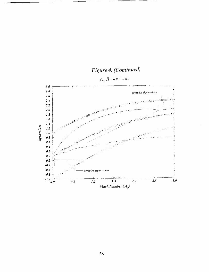
3.0

2.8

2.6

2.,1

2.2

2.0

1.8

1.6

1.4

1.2

1.0

0.8

0.6

0,4

0.2

0.0

-0.2

-0.4

-0.6

-0.8

-1.0

Figure 4. (Continued)

(o). H = 6.0, O = O,1

k

,b •t_

complex eigen values , i

00000000C r" '" i

COD,OC_O0 I

I oO_ ///_ - .....0 - _ £'0- 37

i / _ , ,,a°e°_ ._" ._.c'_'c .... ..

\ i _©L,

.. :, ¢ " _ cotttplex eigen _'alues

0.0 0.5 1.0 1.5 2.0

Mach Number (M e)

2.5 3.0

58

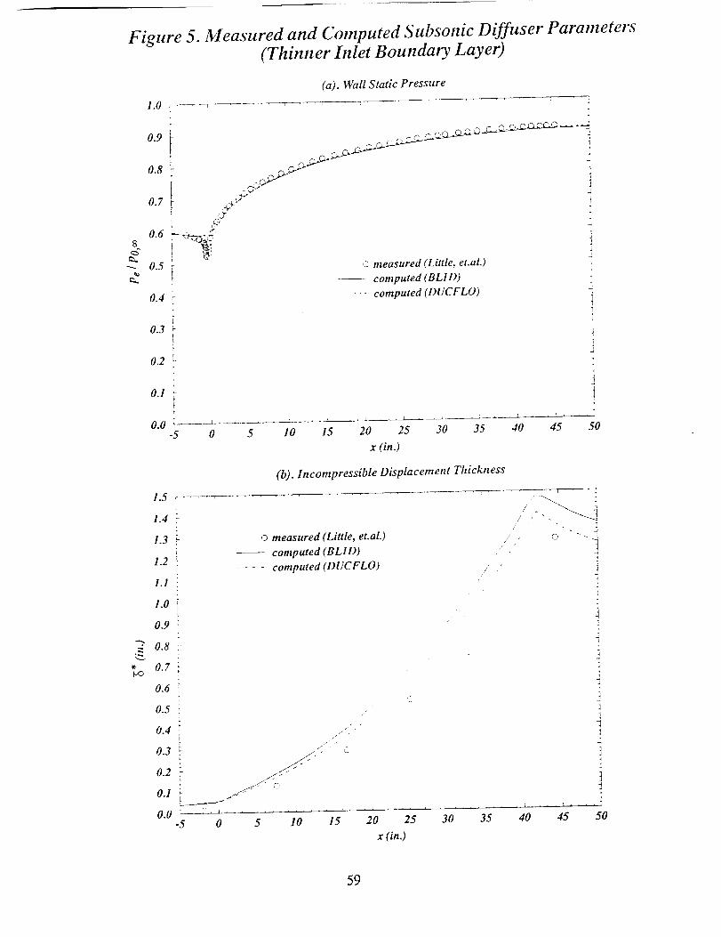
Figure 5. Measured and Computed Subsonic Diffuser Parameters(Thinner Inlet Boundary Layer)

0.68&

0.5

1 °0 _-_

0.9 i

0.8 l

0.7 ,r ,+_J2Y

i

0.4 _

0.3

0.2 !-EI

o.1 ;

0.0 '-'_--_--_-5 0 5

1.5

1.4

1.3

1.2

1.1

(a). Wall Static Pressure

J

_2measured (Little, et.al.)

-- computed (BLID)

..... computed (DUCFLO

10 15 20 25 30 35

x (in.)

(b). Incompressible Displacement Thickness

© measured (Little, et.al.)

computed (BLI D)

.... computed (DUCFLO)

!J

]7

d

q

40 45 50

i

/' " _ H

1.0

0.9

0.8

0.7

0.6

0.5

0.4

0.3

7

r

0.2 !

0.I

0.0 =--:_-_-5 0

J

../_/-/" C;

5 10

C

15 20 25

x (in.)

30 35 40

1

J

.... J

45 _0

59

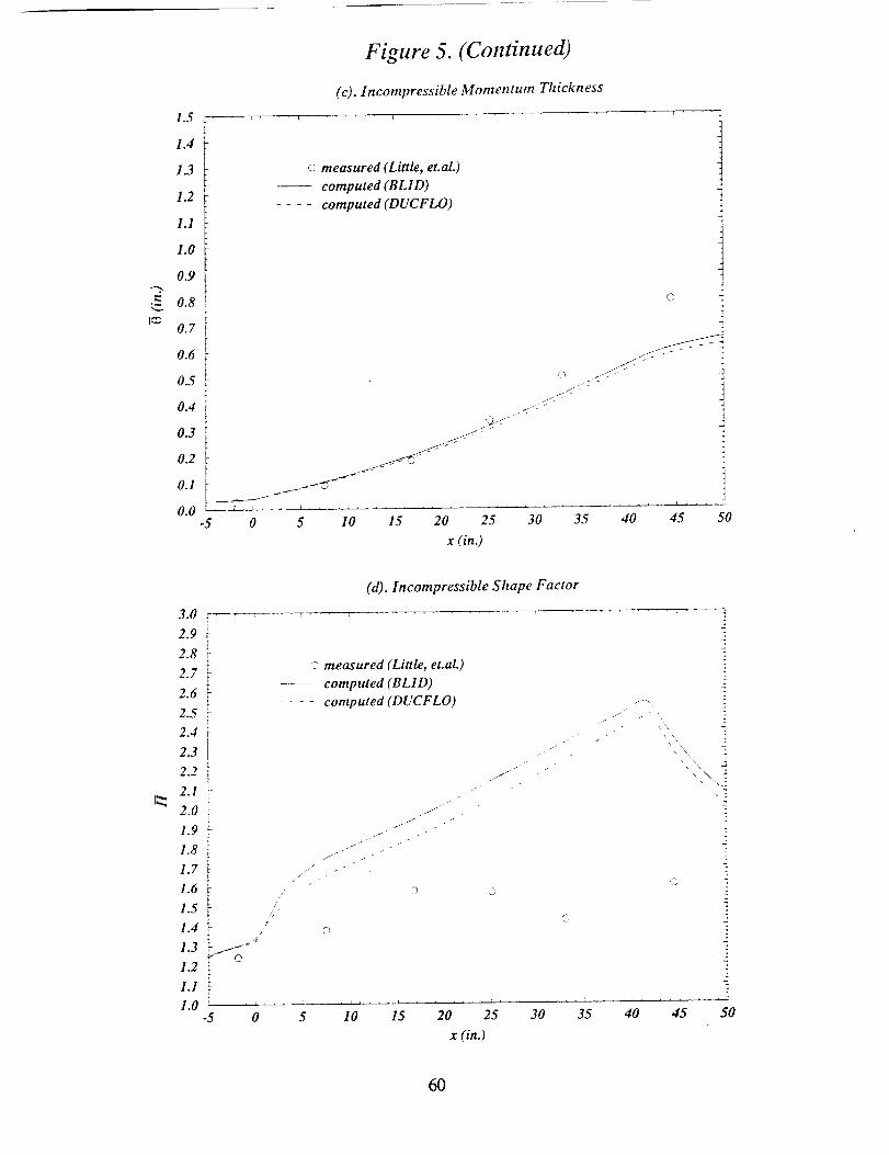
Figure 5. (Continued)

1.5 L .... ' .... 1

1.4 i1.3

1.2

1.1

1.0

0.9

0.8 !

0.7

0.6 _-

0.5

0.4

0.3 _

0.2

0.I

0.0 _-_--_-_-_......-5 0

(c). Incompressible Momentum Thickness

o measured (Little, et.aL)

computed (BLID)

.... computed (DUCFLO)

©.-%

5 10 15 20 25 30 35

x (in.)

]

2

4O

]i .....

45 50

3.0

2.9

2.8

2.7

2.6

2.5

2.4

2.3

2.2

2.1

2.0

1.9

1.8

1.7

1.6

1.5

1.4

1.3

1.2

1.1

1.0

(d). Incompressible Shape Factor

i i

) measured (Little, et.al.)

-- computed (BL1D)

.... computed (DUCFLO)

//

. 1 ¸_/¸. t-

O

J

J

-5 0 5 10 15 20 25 30 35 40

X (in.)

2

, \

2

]

3

t?

45 50

6O

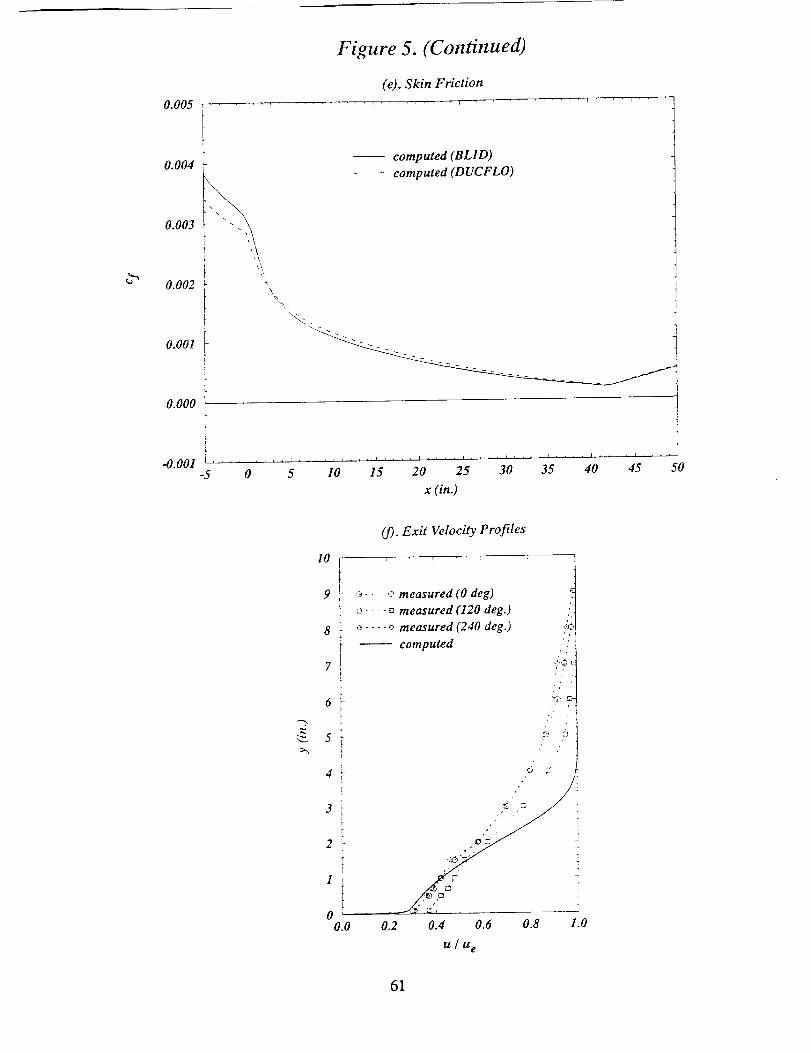
0.005 .... f ' ' • l

Figure 5. (Continued)

(e). Skin Friction

_ .... E , • i .... i " ' " " i .... i ....

0.004

0.003

0.002

0.001 (

0.000

-0.00I

1i

\

-- computed (BL1D)

.... computed (DUCFLO)

i

I[

.... £ .... I .... i .... i .... i .... i .... i ........ i .... i ....

-5 0 5 I0 15 20 25 30 35 40 45

x (in.)

iJi

5O

lO f

9!_IL

8'r

7

6L

5

4 _

3

2

I

LO'

0.0

(J). Exit Velocity Profiles

.... _ measured (0 deg)

.... _ measured (120 deg.)

o .... _ measured (240 deg.)

-- computed

0.2 0.4 0.6 0.8 1.0

u/u e

61

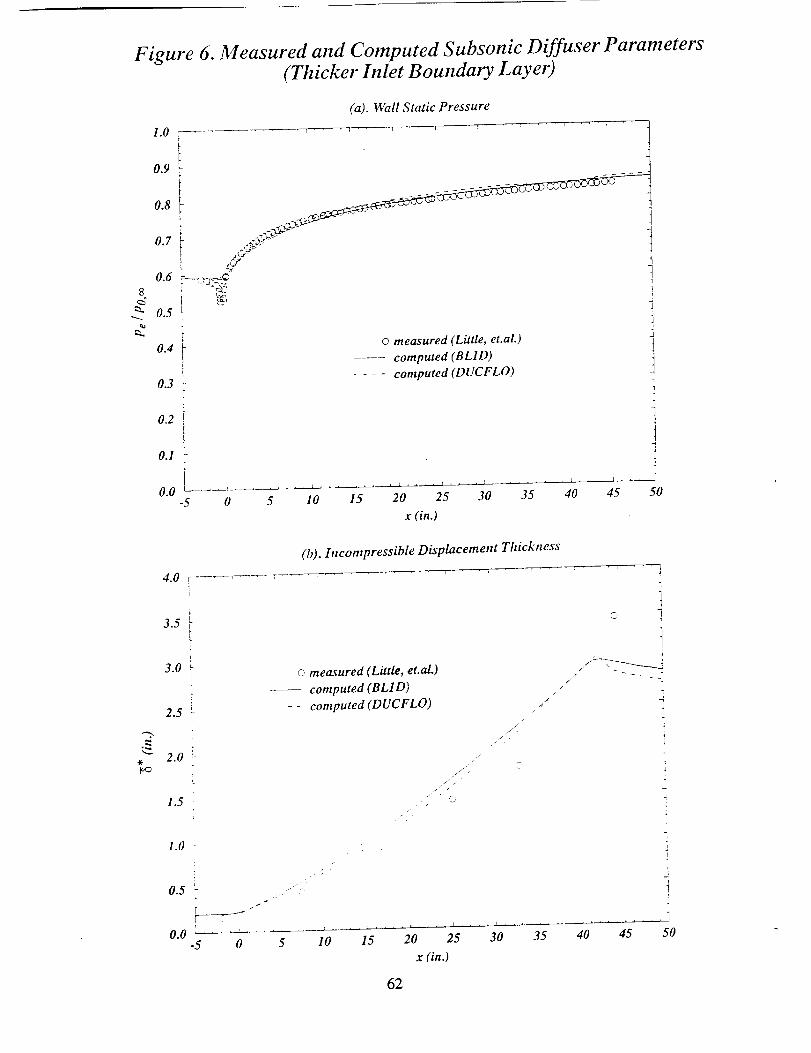
8

ca.

Figure 6. Measured and Computed Subsonic Diffuser Parameters

(Thicker Inlet Boundary Layer)

1.0

0.9

0.8

0.7

0.6

0.5

0.4

0.3

0.2

0.I

0.0

(a). Wall Static Pressure

'r

L

-5 0 5 10

o measured (Little, et.al.)

computed (BL1D)

.... computed (DUCFLO)

t .... t .... + .... i • • + i .... I .... k .....

15 20 25 30 35 40 45

x (in.)

50

4.0

3.5

3.0

2.5

2.0 _-

L

1.5

I,O "

0.5

T--r

0.0 _-5

J

C

(b). Incompressible Displacement Thickness

F r _ - ,, _ • , _ • F • i - i • ] ....

o measured (Little, et.al.)

---- computed (BL1D)

.... computed (DUCFLO)

+

j •

C,

I

J

o 1

i

i][

0 5 10 15 20 25 30

x (in.)

35 40 45

J

i

J

2

50

62

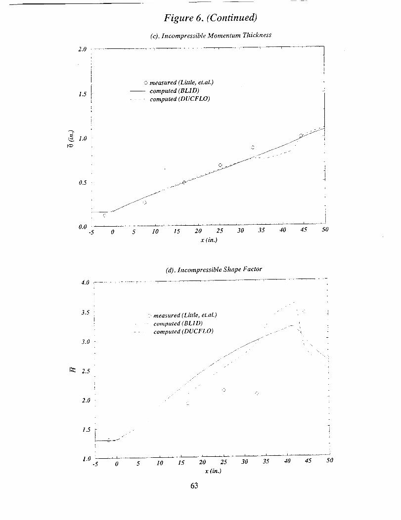
2.0

Figure 6. (Continued)

(c). Incompressible Momentum Thickness

T .... T ' ' _ ' i ' i ' ' r

1.5

""2,.

__ s.o

© measured (Little, et.al.)

computed (BLID)

.... computed (DUCFLO)

oJ_J

0.5 - ._? .1_

I

O0L. _ _ .............. , .............-5 0 5 10 15 20 25 30

J

Ii

d

i

It .... i .... _ , i

35 40 45 50

x (in.)

Izz

(d). Incompressible Shape Factor

4.0 ........ _ ........ : ..... _ , , .

3.5 •

i :, measured (Little, et.aL)- -- computed(BL1D)

computed 'DUCFLO) .

3.0 _ f" -' /

,i. .J

L .1"-/

2.5

2.0

/

//

/

r_:

\,.

1o5 ,>- • .

L

L

__l.rJ_ ,,_ .... _ ....-5 0 5 10 15 20 25 30

x (in.)

63

35 40 45 50

0.004

0.003

0.002

0.001

0.000 i

fr

-0.00I _-5

Figure 6. (Continued)

(e). Skin Friction

r , y j

computed (BLID)

.... computed (DUCFLO)

\\

4

I

JI

-iJ

505 I0 15 20 25

x (in.)

30 35 40 45

lo t

09. Exit Velocity Profiles

s t7 t

6

..->.

"_ 5

4

3

2

1

00.0

,:, .... e measured (0 deg)

_-- - 6 measured (I20 deg.)

:- .... _ measured (240 deg.)

computed

! ,-/o:; i!i _ /"i° J

!-..,#.... .0.2 0.4 0.6 0.8 1.0

u/u e

64

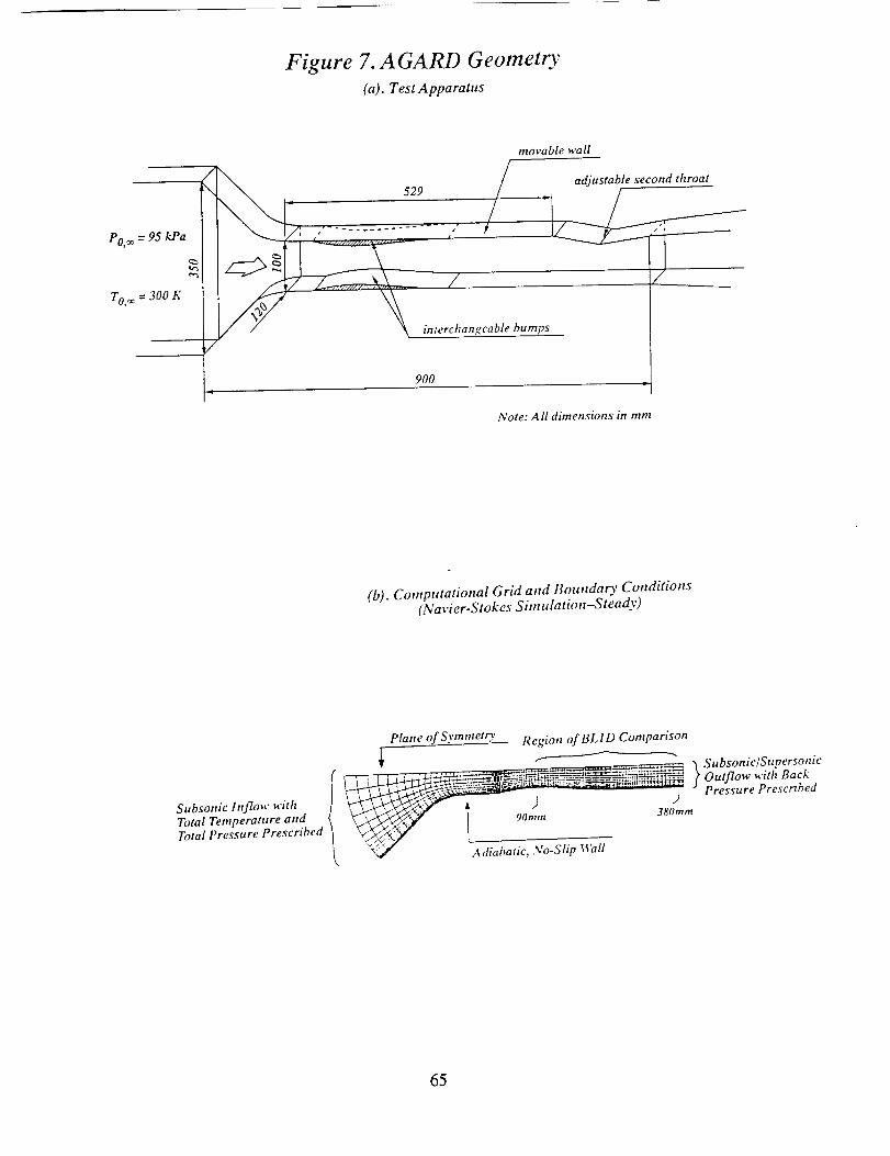
Figure 7. AGARD Geometry

(a). Test Apparatus

PO, _ = 95 k.Pa

e_

TO,_ = 300 K

/

/

movable wall

. 529 / adjastableseeondthroat

te changeable bumps

900

Note: All dimensions in mm

(b). Cotnputationa[ Grid attd Boundary Conditions

(Navier-Stokes Simulation-Steady)

Subsonic Inflow withTotal Temperature attdTotal Pressure Prescribed

Plane of Svtnmetry Region of BL1D Comparison

I _--_ ............. _ .... "1 Subsonic�Supersonic

__ [ Outflow with Back

'_ j _ J Pressure Prescribed

'_c, No-Slip Wall

65

Figure 8. Navier-Stokes and BL1D Comparisons (Steady Case)

(a). Maeh Number

1.8 .....

1.7

1.6

1.5

_ 1.4

e_

:_ 1.3

1.2

I.I

BL1D

o Navier-Stokes

//.

¢>

d

50 100 150 200 250 300 350

x (ram)

(b). Density

J

i

400

0.7 f

0.6 !

0.5 !

k

0.4 _

F

o.3 _-r

E

o.2 !5O

BL1D

o Navier-Stokes

\X

1 1 ! .... J , , , !

I00 150 200 250 300 350

X (ram)

400

66

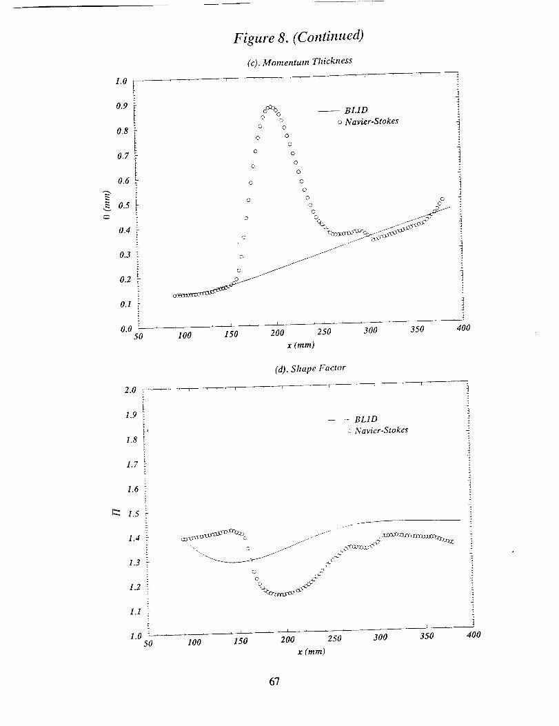
0.8

0.7

0.6

= 0.5

0.4

0.3

0.2

t

0.I

0.050

2.0

Figure 8. (Continued)

(c). Momentum Thickness

i i

oC%© 0

©

0 ©

0 0

Q

00

00

0

© 0

0

0

',3

0

t I t

-- BLID

o Navier-Stokes

]

0 0 -_© 0

ss

32

100 150 200 250 300 350 400

x (ram)

(d). Shape Factor

i , " I F

1.9

t,

1.8

1.7

1.6 --

I_,, 1.5

1.4

1.3 -

1.2

1.1

1.05O

-- BLID

o Navier-Stokes

I00 150 200 250 300 350

x (ram)

z

400

67

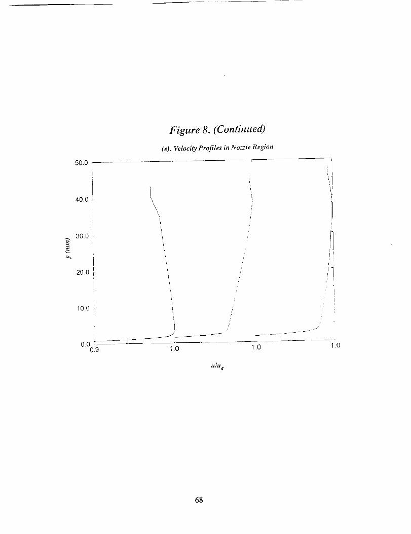
50.0

40.0

30.0

20.0

10.0

Figure 8. (Continued)

(e). Velocity Profiles in Nozzle Region

i

i\\

/ j_

l,i

i

t!J I

0.00.9 1.0

u/u e

1.0 1.0

68

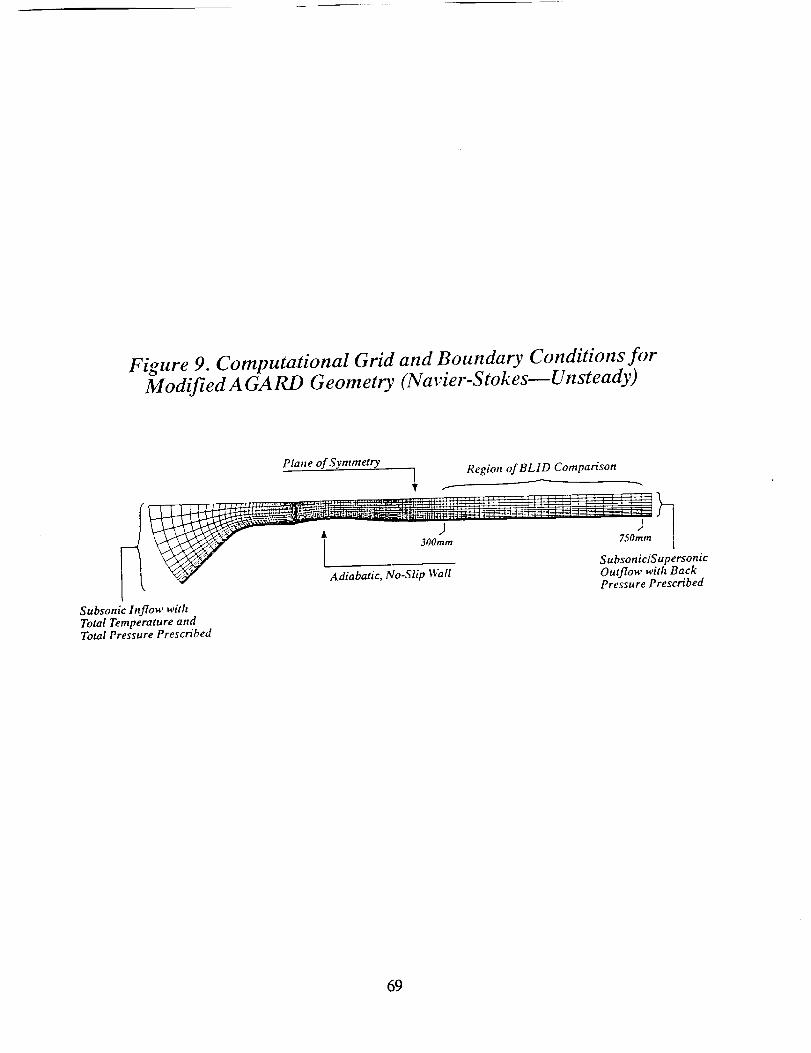
Figure 9. Computational Grid and Boundary Conditions for

Modified A GARD Geometry (Navier.StokesmUnsteady)

Plane of Symmetry

Region of BLID Comparison

(I I I I __:_:T_ i ["'_:':'!!",i _i _ii i] _ , _ i "_

I ____'_,-_,-,L_F

300ram 750ram

I [ _J(_" I .... , Subsonic/Supersonic

[ L _ Adiabatic, No-Slip Wall Outflow with BackI Pressure Prescribed

Subsonic Inflow withTotal Temperature andTotal Pressure Prescribed

69

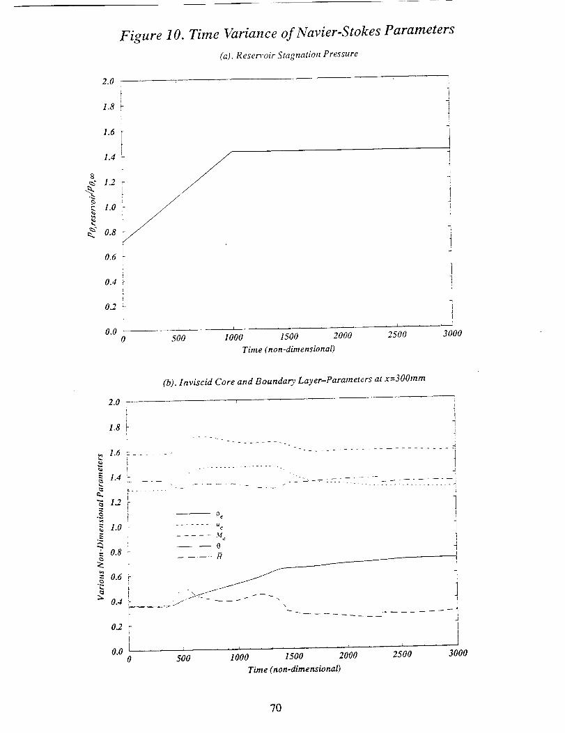
Figure 10. Time Variance of Navier-Stokes Parameters

(a). Reservoir Stagnation Pressure

2.0

1.8

1.6

1.4

8

,_" 1.2

_ 1.0

_" 0.8

0.6

F

F

0.4

0.2

0.0 J

0 500 1000 1500 2000

Time non-dimensional)

2500 3000

2.0

(b). Inviscid Core and Boundary Layer-Parameters at x=3OOmm

!

1.8i

_. 1.6-_ .......e _

1.4 _ ....

"_ 1.2

= 1.0e_

._.

" O.8

t_

_ 0.6:

0.4 ;,

O2

0.00

Pe i

M " i

oR r

/

/,\

500 1000 1500 2000

Time (non-dimensional)

2500

i'.J

3000

7O

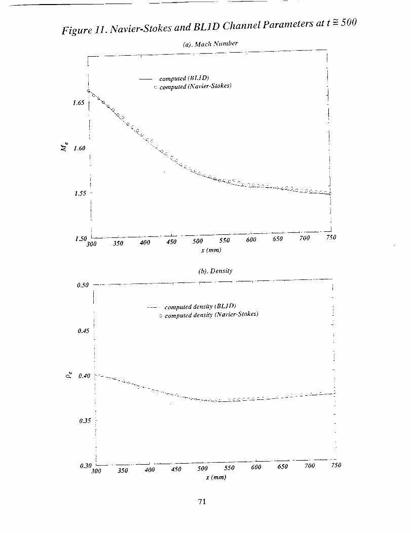
Figure 11. Navier-Stokes atzd BL1D Channel Parameters at t = 500

(a). Mach Number

i i --7 " i

JL

5\

1.60 _[

L

f

1.55 _

I

1.503O0

-- computed (BLID)

o computed (Navier-Stokes)

350 400 450 50 550

x (ram)

_ ]

CC_- i

Ji

J

I t ._J

600 650 700 750

(b). Density

0.50 _ i

C

0.45

computed density (BLID)

o computed density (Navier-Stokes)

400 450 500 550 600 650 700

X (mm)

]]

J

750

71

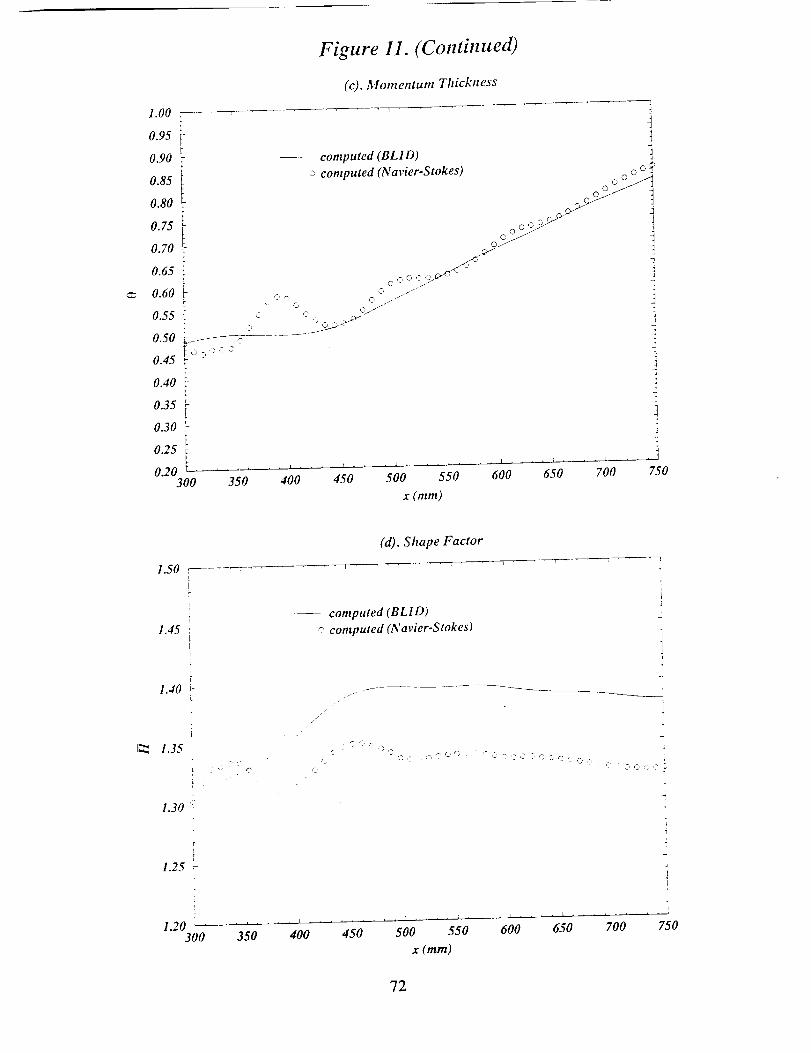
1.00

Figure 11. (Continued)

(c). Momentunz Thickness

0.95

0.90

0.85

0.80

075[0.70

0.65

0.60 F

0.55 i©

0.50 _._ ,=

0.45 rk

0.40 L

0.35

0.30 F

0.25

0.20 r .........300 350

C' © 0

computed (BLI D)

o computed (Navier-Stokes)

0 J':"

0 © -J/

00 0__ '

oo/ 4

c_ 40I_ 4

@..i

i .... t ] 1 L I L . • _

400 450 500 550 600 650 700 750

x (ram)

1.50

(d). Shape Factor

1.45 ,L

F1.40 _-

1

F

L

_, 1.35

1.30 F

i

1.25

L

1.20 i .3OO

• Q £ © .:

.... computed (BLID)

c computed (Navier-Stokes)

/://

C, - 0 ,_

:2:_ C: C '2' C : 'C C, '2 : :., 2

- _ _, ,2 '-" 0 C ? -,,'

, . ..... L , , , , ]

350 400 450 500 550

x (ram)

600 650 700 750

72

Figure 12. Navier-Stokes and BL1D Channel Parameters at t -- 1000

(a). Math Number

1.75

1.70

0000000000000___

00_ - _uW<JOOC, oo

O+J0 /

i @_/'/

k1.65 I

f

L

iL

1.60 U .....300 350

computed (BLID)

o computed (Navier-Stokes)

t .... i t i L t

400 450 500 550 600 650 700 750

X (ram)

(b). Density

0.58

0.56 :

0.50

0.48

0.46 -

computed (B L 1D)

o computed (Navier-Stokes)

0.44 7-

0.42 F

0.40 L.......... + .... + .................300 350 400 450 500 550 600

x (mm)

650

J

700 750

73

Figure 12. (Continued)

(c). Momentum Thickness

1.2 ,t

1.I

1.0 I

0.9 l

o.8 _

_ o.7"

computed (BL1D)

o computed (Navier-Stokes)

0

, 00.6 _ c

0.5 _

ir 0

0.4

[

0.3 _r

02 ....

0

CO

< _ 0 c /

00 GO O0 ":' _ _

i

]

1

000000000_

o l

o°

300 350 400 450 500 550 600 650 700 750

X (ram)

1.50

1.45

1.40

(d). Shape Factor

l .... "i "

-- computed (BL1D)

c computed (Navier-Stokes)

1.35

1.30

//

& 0 'D L

_ _ #: C¸

GO0 0 0 0 ,_ _ C' _ -

O 0 'D C D t t0

1.25 -

1.20300

i .... , .... 1 .... _ t

350 400 450 500 550

x (ram)

i

4

!

4J

J

Ji t

600 650 700 750

74

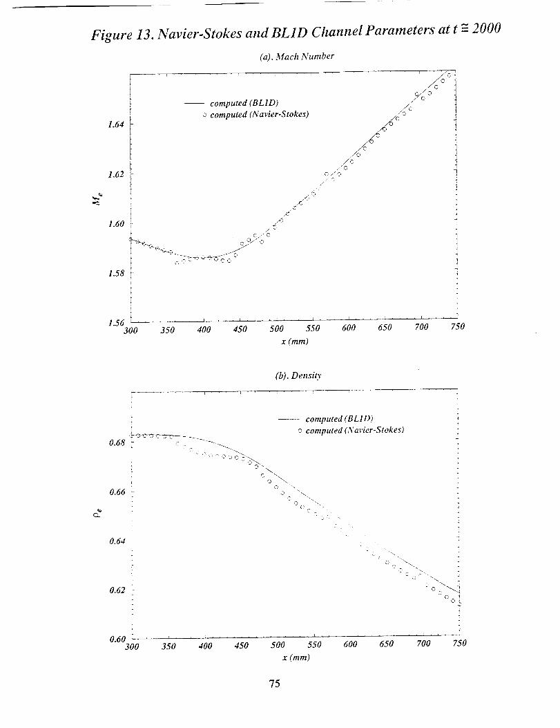
Figure 13. Navier-Stokes and BL1D Channel Parameters at t -- 2000

(a). Mach Number

_a

[r

1.64 f

1.62 It

t1.60 qc

1.58 i

kL

1.56 _

-- computed (BLID)

o computed (Navier-Stokes)

,C

xT;

C./" 0

300 350 400 450 500

./0

C'/" 0

// 0/

... %'

550 600

! .... k ....

650 700 750

x (ram)

(b). Densit)'

0_

kr

0.68 c : ,:- _'_'_.

r_

0.66

0.64

0.60300 350 400 450

--- computed (BLID)

o computed (Navier-Stokes)

0 "\

500

C C, -,4o _

550 600 650 700 750

x (ram)

75

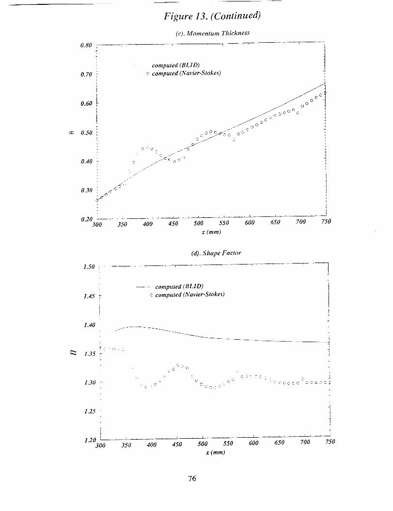
0.80

0.70

0.60

0.50 L

0.40

u

0.30 _ f

L

0.20 L..... __300 350

C:

//

Figure 13. (Continued)

(c). Momentum Thickness

0 C 0?

..._© C' 0

/

computed (BL1D)

o computed (Navier-Stokes) 1

°O°O0 - i

!°_6_, o'-'

0 .. !

I '

4n

i

5

3

400 450 500 550 600 650 700 750

x (ram)

1.50

(d). Shape Factor

T

I

L

1.45 F

L

1.40ir

!

k _" 7' 0 - 1

1.35 -

t.3o

?k

125 r7

L

1.20 ......300 350

computed (BL1D)

o computed (Navier-Stokes)

O C, ,2'5 C

CC,

C 30

C

C C, ,2

00 ,2 C

L ,I I

400 450 500

C

O D '2 C, ,5_ -- C _ C

'- COocO

J1'I

J

!

q1

fi!JI

I

I

J00000,_

J

I

I3

4550 600 650 700 750

x(mm)

76

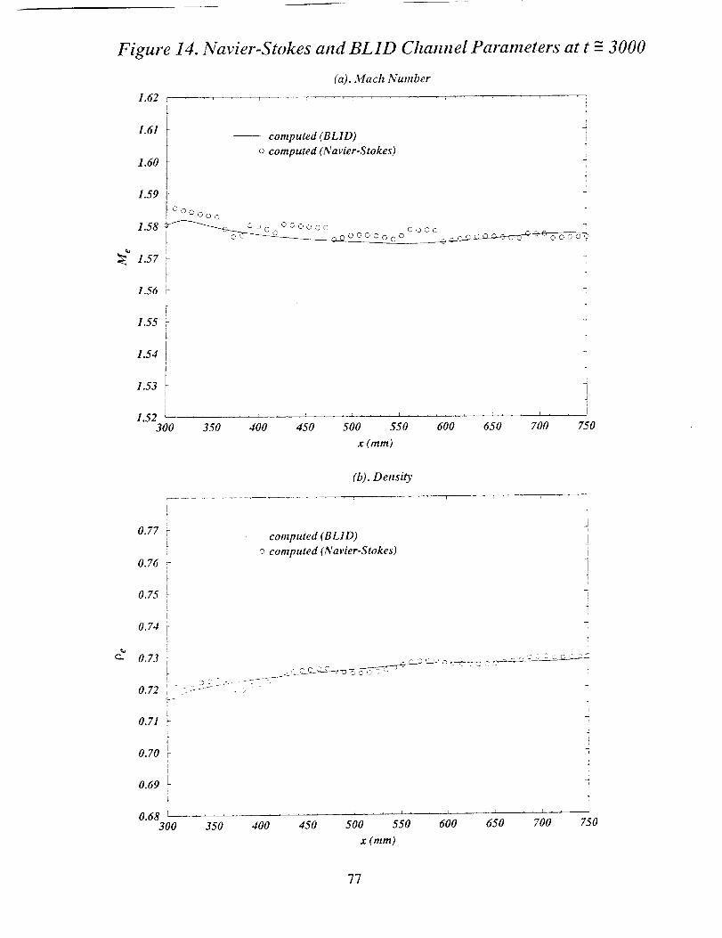
Figure 14. Navier-Stokes and BL1D Channel Parameters at t =-3000

(a). Math Number

1.62

1.61

1.60

1.59

computed (BLID)

o computed (Navier-Stokes)

F[

O00oo0

1.58 _...._G_, 0 OOo00C

i1.57 !-

[1.5s i

1.54![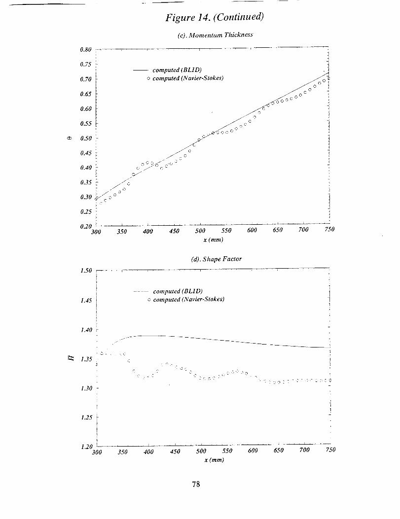

1.53 !J

1.52 i3OO

1.56

COOG0

350 400 450 500 550

x (mm)

, , J 1

600 650 700 75_

C

I

0.77i

0.76 _-

I0.75 "

I

I

0.74 i

0.73 .r

o.72 [-=)._- :.... _ __

0.71 _iI

0.70

0.69 L

___0.68_ .... , ,300 350

(b). Density

- -- computed(BL1D)

o contputed (Navier-Stokes)

400 450, i I

500 550 600 650 700 750

x (mm)

77

Figure 14. (Continued)

(c). Momentum Thickness

0.80

0.75 _-

0.70 ,-

0.65

0.60

'r0.55

0.50

0.45

0.40

0.35

0.30

0.25

0.203O0

i 0Ui

_- tf'_

[ /"oo '_>,_co

iro

4

icomputed (BLID) . j.

o computed (Navier-Stokes)

_a ° ° ]

,. -->>'_°°°° _ ]

C' 0 _-/_ , Co j.o o o

350 400 450 500 550 600 650

x (ram)

700 750

1.50

(d). Shape Factor

1.45

1.40

1.35

1.30

1.25

L

1.20300

._J

C

,7

,} g _ C,

350 400

computed (BL1D)

o computed (Navier-Stokes)

0 C: ,3 -

- 0 C;,D ,Z....

C' _O_ _ 0 -'2 C C '-" '_ " ,D

iII

i

i

I

- '_- T 3 0 5, : :2 d _." ,_- C :3 C C',

45O 500 550 600 650

x (ram)

r

700 750

78

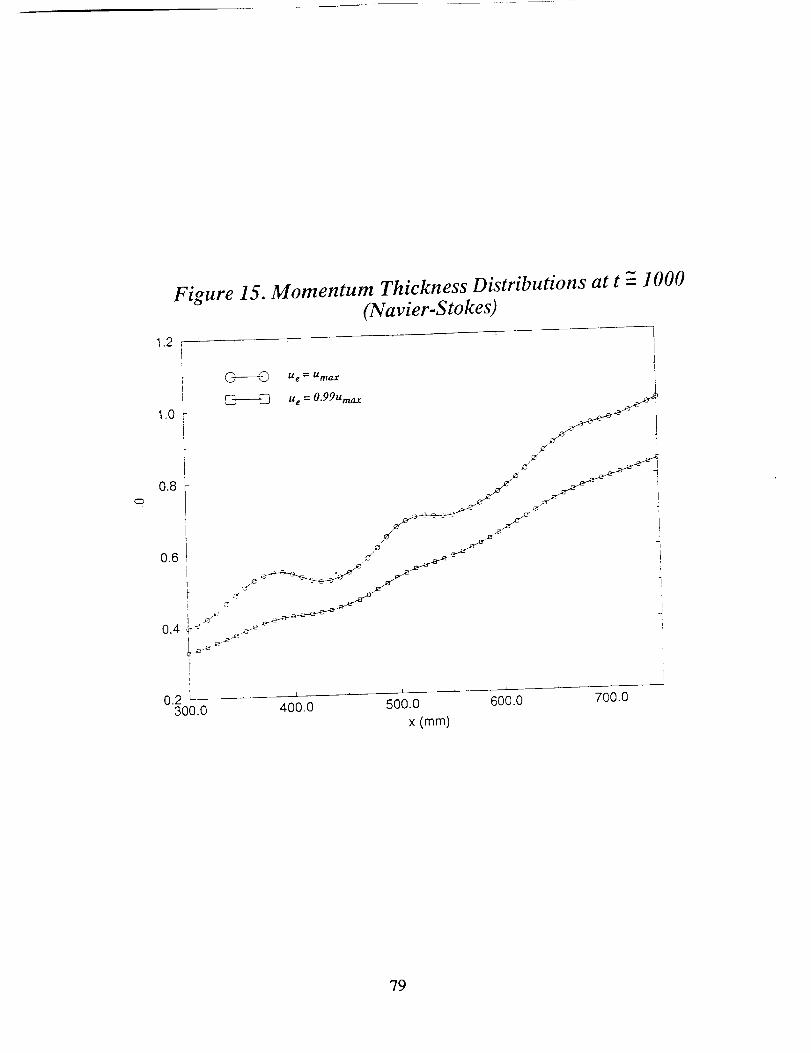
Figure 15. Momentum Thickness Distributions at t ---1000(Navier-Stokes)

1 .2 _ r--i

II

! _ tte=UmaX

I

1.0 i _ ue = 0"99Umax

0.8

,-e'0.6 !L1

!

0.4 4_'e- .,__

1

0.2"300.0

[J

JJit

J

II

400.0 500.0

x (mm)

600.0 700.0

79

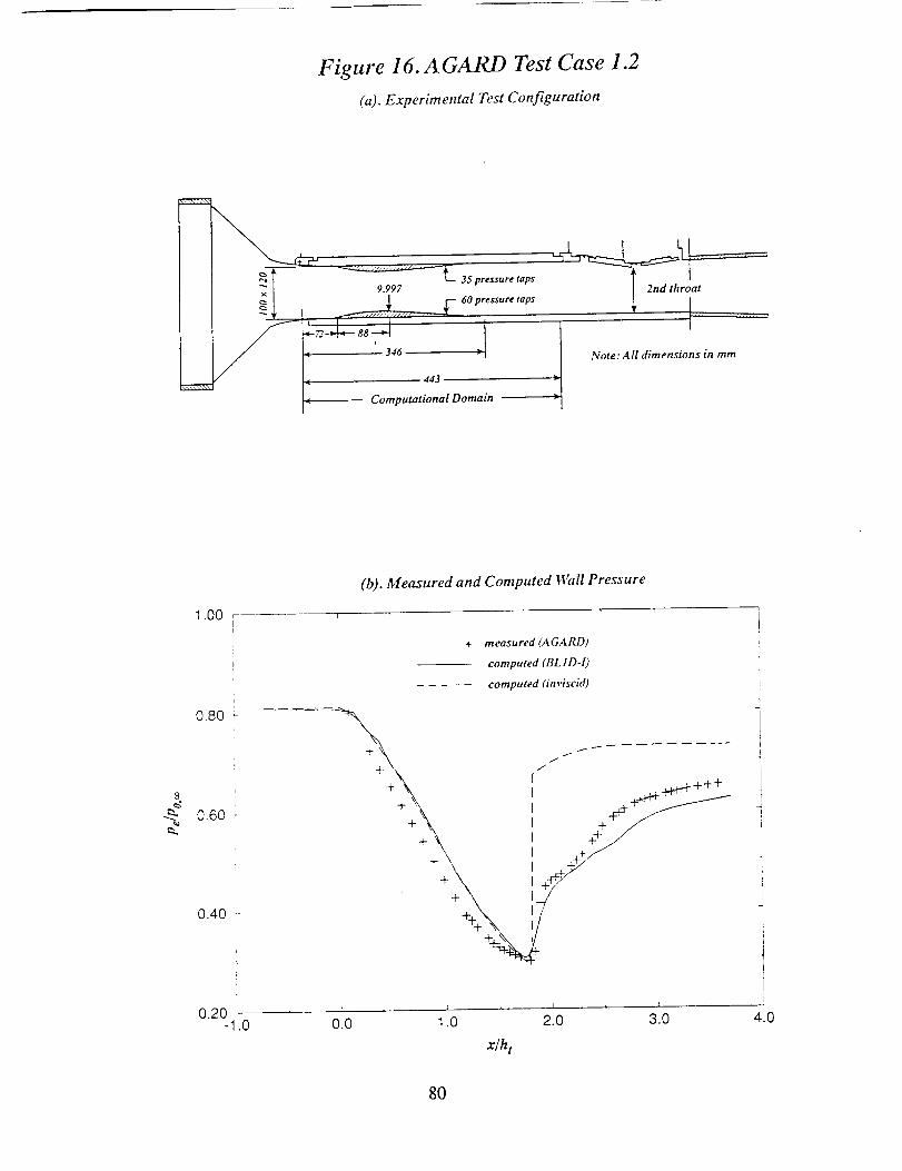
Figure 16. A GAI_ Test Case 1.2

(a). Experimental Test Configuration

_ I _ 35pressure taps

9.997

_ _-- 60 pressure taps[

_l Note: All dimensions in mm

1.00

(b). Measured and Computed Wall Pressure

8

0.80

0.40

+ measured (A GARD)

computed (BL 1D-I)

comptited dn viscid)

+ \ ,_a-N-.++ +

+ \ _+,-_+_LS------_+ ,\ +++T_

÷ \ ÷_-J+ \ ,++_

0.20 I , _ _ ,-1.0 0.0 1.0 2.0 3.0

x/h t

4.0

80

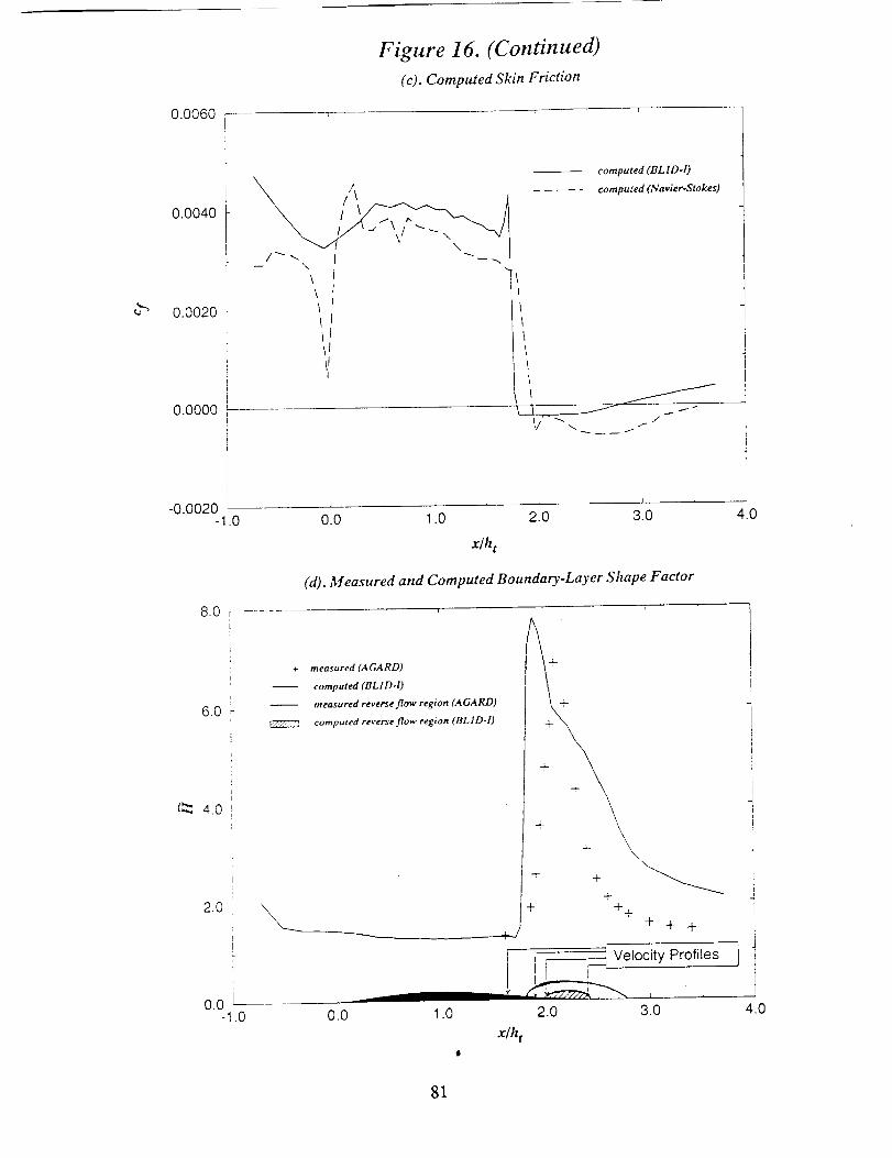
0.0060

Figure 16. (Continued)

(e). Computed Skin Friction

0.0040

0.0020

0.0000

-0.0020.0

8.0 r

computed (BL 1D-I)

/ computed (Navier.Stokes)

--/ _ " \\\ ! "" _ " l lI

_/ "- /

J

Jf

0.0 1.0 2.0 3.0

x/h t

(d). Measured and Computed Boundary-Layer Shape Factor

4.0

6.0_

[_ 4.0

2.0

i

J

o.o L-1.0

measured (AGARD)

computed (BLID-I)

measured reverse flow region (AGARD)

computed reverse flow region (BLID-I)

++

0.0 1.0

4-

4- .4-

1

4-

4.- j

4-+

4-++

[ t ,

2.0 3.0

x/h t

t Velocity Profiles ]

4.0

81

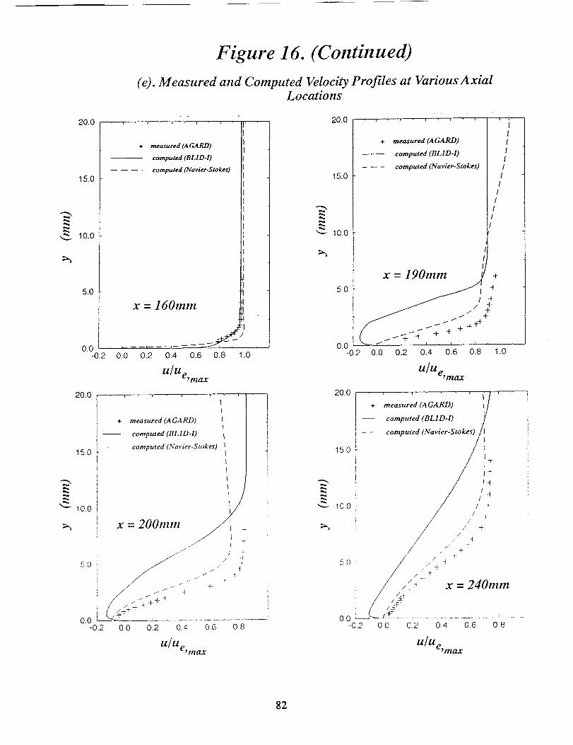
20.0

15.0

210.0

5.0

0.0-0.2

20.0

150

"_ 100

Figure 16. (Continued)

(e). Measured and Computed Veloci_ Profiles at Various Ax_lLoe_ions

..... 20.0 .....

measured (A GARD)

computed (BL I D-I)

computed (Navier-Stokes)

IiIx = 160tnm

j'I

0.0 0.2 0.4 0.6 0.8 1.0

U/U e, max

50

0.0

m ea su red (A GA _)

comp_ed (BLID-I)

computed (Na vier-Stokes)

x = 200mm

./i

J _

i _ _ t '

d/ 4f

J 4

+

4

-0.2 0.0 0.2 0.4 06

U/Ue_max

0.8

15.0

lO.O

5,0

0.0-0.2

t50

"_ +o+o

measured (A GARD)

computed (BLID-I)

computed (Navier-Stokes)

'iI1I

I//

I//

/Ir

Ii

x = 190mm ) +

_ _" -t-

k,.._ ,..-_ 7-. , .......

0.0 0.2 0.4 0.6 0.8 1.0

U/Ue, max

20.0 .... L [+ measured (A GARD) I

computed (BLID-I)

computed (Na vier-Sto kes) / Ii

/,

////44 +

50 ..,, _

x = 240mm

/ ,Zo0 -d-2 ..............

U/Ue, max

82

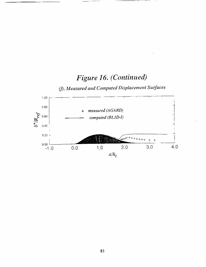
1.00

Figure 16. (Continued)

09. Measured attd Computed Displacement Surfaces

0.80

*_,0 0.40

measured (A GARD)

computed (BL1D-I)

0.20

r

o.ooL_-I.0 0.0 1.0 2.0

x/h t

_+++ + +

3.0 4.0

83

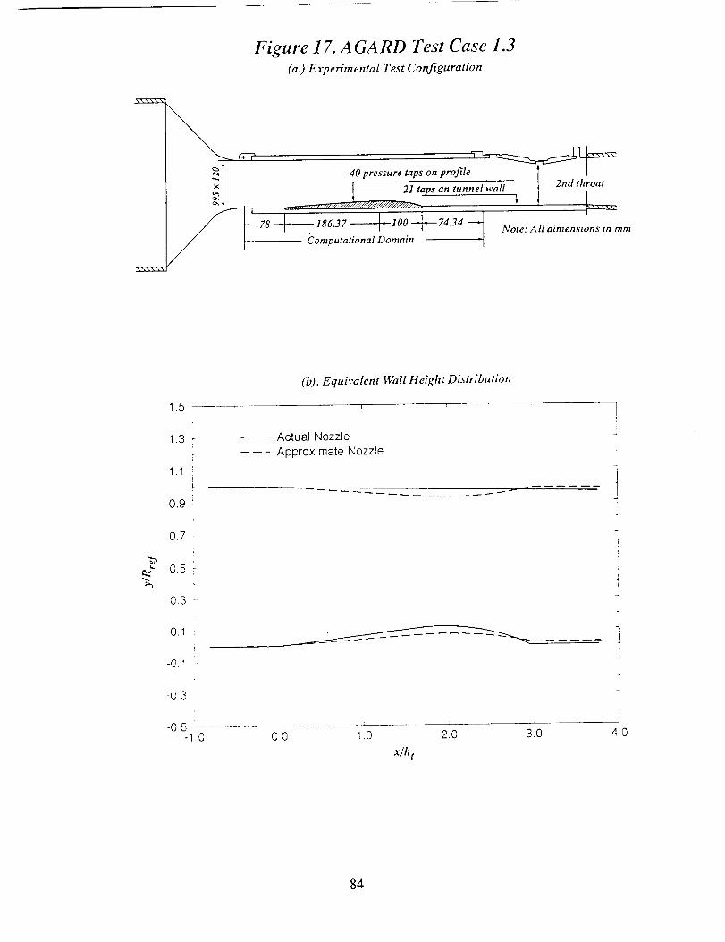
SXXXSS

Figure 17. A GARD Test Case 1.3(a.) Experimental Test Configuration

_,_ _u==2 [ 40 pressure taps on profile l t

. . . . .

1.5 _

(b). Equivalent Wall Height Distribution

!

i

1.3

1.1

0.9

0.7.

0.5_L

0.3 r

0.1 '

-0.1

-0.3

Actual Nozzle

----- Approximate Nozzle

-0,5 ......-1.0 0.0 1.0 2.0 3.0 4.0

x/h t

84

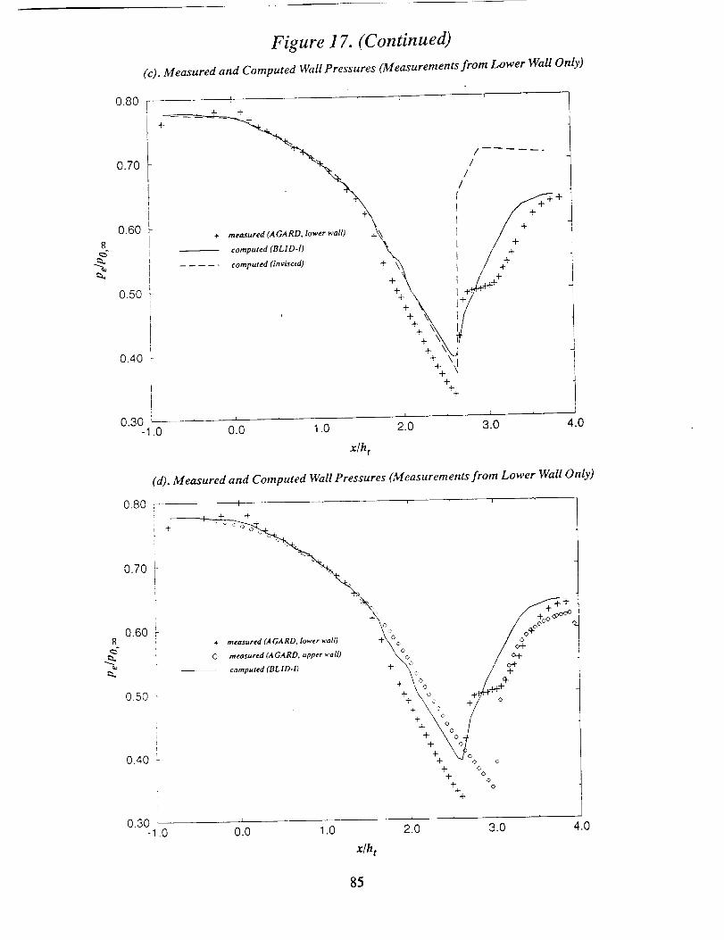
Figure 17. (Continued)

(c). Measured and Computed Wall Pressures (_leasurements from Lower Wall Only)

0.80 I ,

8&

h,

0.70

0.60

0.50

0.40

0,30

. i/I+

+ measured(AGARD, Iowerwall) +_ / L +

" " c°mputed (BLID'l) X /

--- - computed (inviscid) + % / +4-

\\' +\ 1_

ai" +

++

I I I

.0 0.0 1.0 2.0 3.0 4.0

xlh t

(d). Measured and Computed Wall Pressures (Measurements from Lower Wall Only)

0.80 I , ,

8

0.70

0.60

0.50

0.40

0.30

• 4- 4-

+ \% / ._4-\.. 4-4+_"

\v;. 7,++yoo/++\_.

+ °o o

+ o+ o

+ o,3

+4-

-1.0 0.0 1.0 2.0 3.0 4.0

x/h t

85

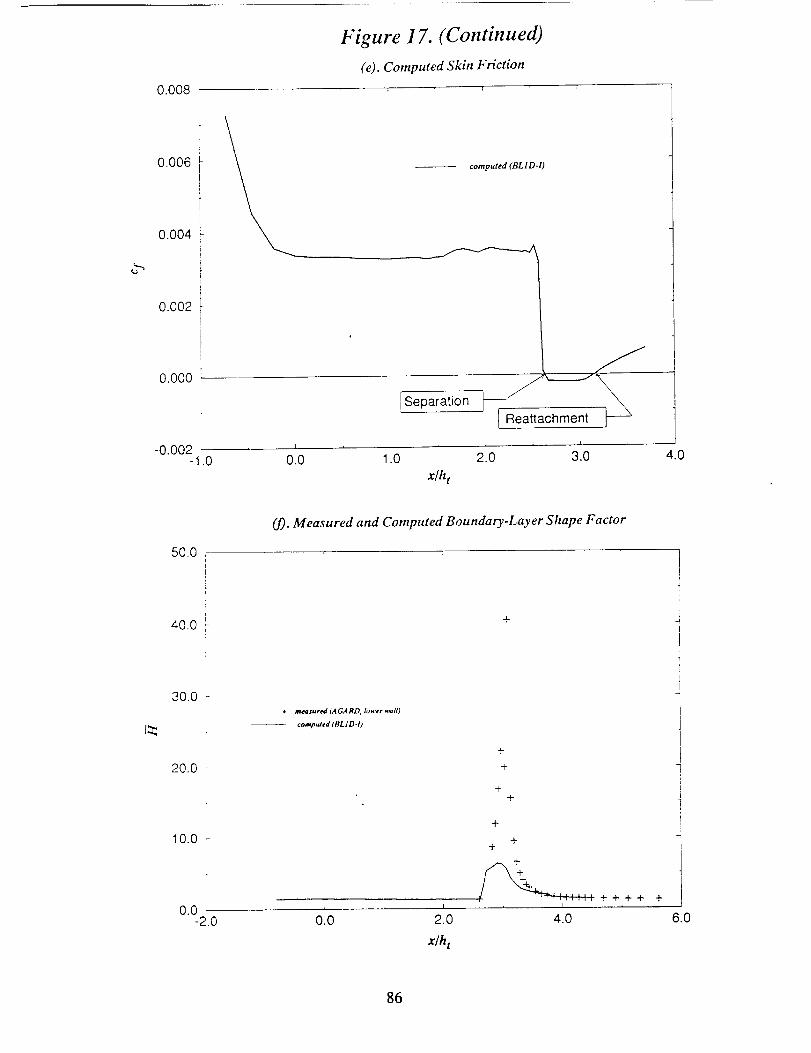
0.008

Figure 17. (Continued)

(e). Computed Skin Friction

0.006

0.004

0.0O2

0.000

computed (BLID-I)

Separation

I I

0.0 1.0

x/h t

f ea.aohmen,

2.0 3.0 4.0

50.0

40.0

30.0 -

20.0

10.0

i

0.0'-2.0

(_. Measured and Computed Boundary-Layer Shape Factor

+

._ rncct$1ared (AGARD, lower .._ll)

computed [BLJ D-D

I I

0.0 2.0

x/h t

+

+

4-

+

+

++

I++++

4.0

86

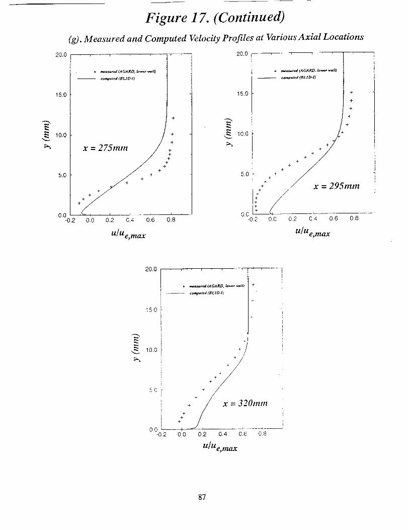
20.0

15.0

10.0

5.0

0.0-0.2

Figure 17. (Continued)

(g). Measured and Computed Velocity Profiles at Various Axial Locations

i • i i

+ tnrcsurcd (.4 CA RD, lo_r wall)

computed (BLI D-I)

+

x = 275mm /

0.0 0.2 0.4 0.6 0.8

U/U e, max

20.0 ....

. measured (AGA R.D, lo_¢r ",,,,'alO

computed (BLID4)

15.0 ++

+

.4-

_ 10.0 + _+

÷ +

+ + "+

5.0 +* +

0.0 _t L-0.2 0.0 0.2 0.4 0.6 0.8

U/U e, max

20.0

15.0

IO.O

5O

O0 k

-0,2

i l i i

÷ me.cured (AGA RD, loa_er wall)

¢oe_uted (BLI D.I)

+

-r

+ -_ _r +

Ol71ltl

/+

0,0 0.2 0.4 0.6 0.8

U/U e,max

87

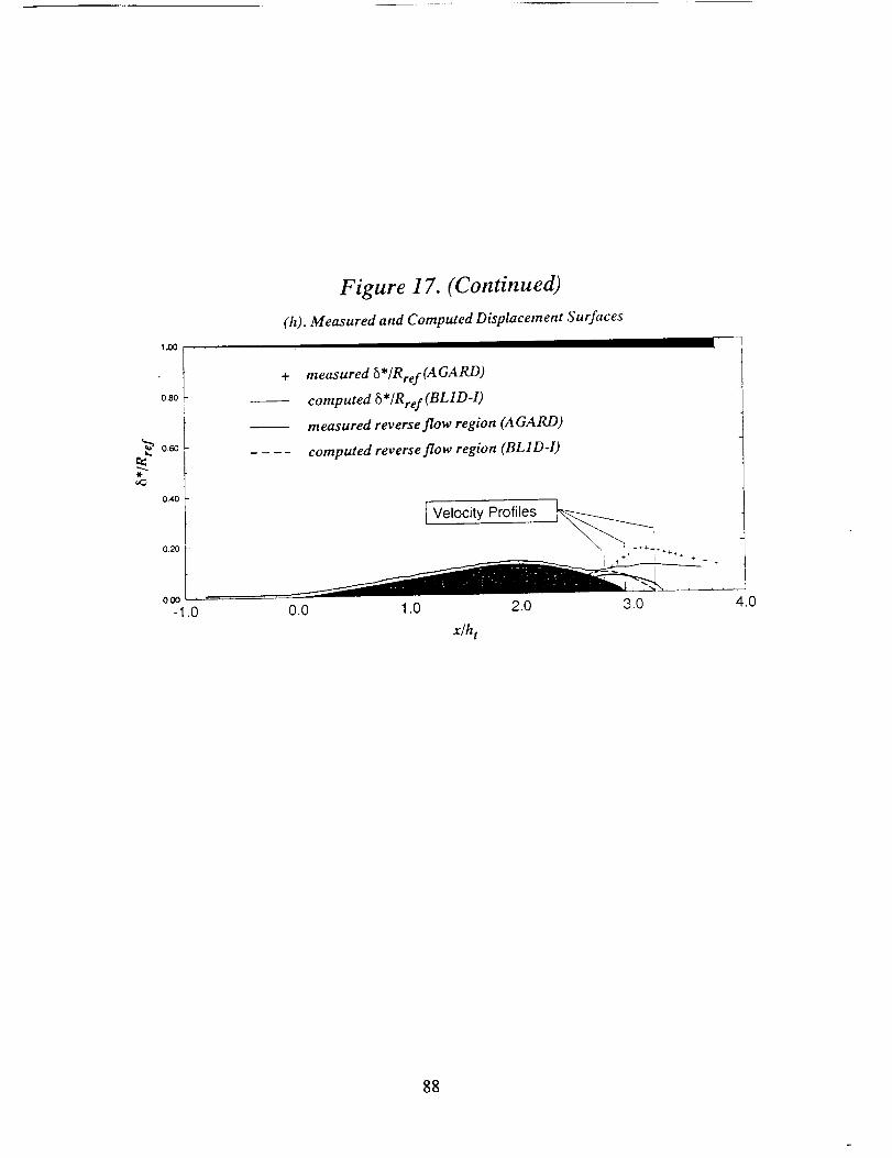
1.00

0.80

0,60

0.40

0.20

Figure 17. (Continued)

(h). Measured and Computed Displacement Surfaces

+ measured 5 */Rre f (A GARD)

comp uteri 6 */Rre f (BL 1D-I)

measured reverse flow region (AGARD)

computed reverse flow region (BLID-I)

t Velocity Profiles

0.0 1,0

x/h t

2.0 3.0 4.0

88

APPENDIX

I. Elements of the L and N Matrices

Recall that the system of equations can be written as

or, in quasi-linear form,

L_-_qt = b (A.I.1)

L_t + N_xx = d (A.I.2)

Elements of the L and N matrices are given below for all formulations and were obtained using the

auxiliary relations reported elsewhere in this Appendix. Each particular element is referred to by

either lower case e (for L) or n (for N) using double subscripts (ij), where i and j represent the specific

matrix row and column, respectively.

Listed first are the L and N matrix elements resulting from the dependent variable vector given by

q = (Oe Ue Me 0 i_) T

A A

Although the ratio To, e = TO,e/To, _ appears in several terms, all computations using this formula-

tion have been made using the assumption To,e = 1. It should be further noted that additional terms

involving derivatives of this quantity were neglected in the original formulation, i.e.,

aTo,e aTo, e- -'0

Ot Ox

L Matrix Using M. as Dependent Variable (T0,e assumed constant)

/11 = ueO (Hs. - Hoo)

/12 = QeOHs"

113 = 2QeueMe0 (c5ff + c 6)

114 = QeUe(Hs" - HO_)

/15 = OeUeO(1 + csM 2)

/21 = Ou2( 1 + H6" - HO_)

l_ = 2Qeu2eMeO(cs-H + c 6)

89

124 = Qeu2( 1 + H_. - HO )

/25 = Qeu20(1 + c5 M2)

131 = A

132 = 0

/33 = - 2QeMe0_ (ClH'+ c2)

134 = Qe_H_.

/35 = - ee0_(1 + ClM2e)

141 = ueA

/42 = 0eA

/43 = - 2QeueMeO_ (ClH + c2)

14a = - QeUe_H6.

145 - -QeUe0W(1 + clM 2)

/52 = QeueA

153 = - 2(Ee + pe)_--"OMe (ClH + c2)

/54 = - (Ee + pe)_H 6.

/55 = - (Ee+Pe)iTiTO (1 + Cl M2)

A p eM eT o,e

N Matrix Using M° as Deoendent Variable (T0,e assumed constant )

nil = OU2

n12 = OeUeO(H,_. + 2)

hi3 = 0

1114 = Qe u2

n15 = 0

n21 = Ou3eHo.

n22 = Oeu_O 3H o.+ 2Ho.- 2

300Ho"n23 = QeUe "_e

n24 = oeuaHo .

90

OH o.

n25 -- QeuJeO--_.-

n31 = ueA

n32 = QeA

n33 = - 2e:ivt:w(cfl" + cz)

,134 -" _ Qeue_H O.

n35 -" - OeUeOW--(1+ clM2e)

n41 = A[(7 - 1)_eTo, e + U2e]

n42 = _eu,A

n43 = _ 2Qeu2OMeW(cl- _ + c2 ) - -_'- 1AQeMe.__eTO,e

n4n = _ OeU2e_H6.

n45 = - Oeu2eOW(1 + clm2e)

( 12)n_1 = ueA 7_eTo, e + _Ue

n52 = A(Ee + Pe + Q_2e)

n53 =

n54 =

n55 =

- 2(Ee + pe)ue_OMe(clH + c 2)

-- (Ee + pe)ue_H 6.

- (Ee + pe)u,iX_9(t + clM 2)

Q eu eM eA

_e To'e

Also, the following definitions have been used:

= 0.113

= 0. 290

= 0.185

C 1

C2

C3

c 4 = 0. 150

C 5 : C 1 -- C3

C 6 = C2 -- C 4

A = w(R-&*)

_ 2, planarW= 1 *

'_ (R - di ), axisymmetric

91

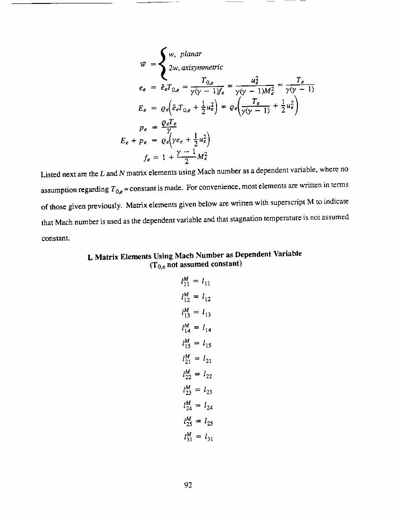
w, planar= 2w, axisymme_ic

To,e u_ Te

e, = _eTo, e Z(?- 1)fe ?(y- 1)M_ y(y- 1)

12) (Te 12)Ee = Oe eeTo,e + _Ue = Oe y(y'_ 1) + _Ue

OeTe

Pe= Y( 12)Ee+Pe = Pe yee+'_Ue

fe = 1 + _-TMe 2

Listed next are the L and N matrix elements using Mach number as a dependent variable, where no

assumption regarding To, e = constant is made. For convenience, most elements are written in terms

of those given previously. Matrix elements given below are written with superscript M to indicate

that Mach number is used as the dependent variable and that stagnation temperature is not assumed

constant.

L Matrix Elements Using Mach Number as Dependent Variable

(To,e not assumed constant)

1_ = 11i

lM = 112

l M = 113

l M = 114

llM5 = 115

1_ = 121

I_2 = 122

l M = 123

12M4= 124

IM = 125

IM = 131

92

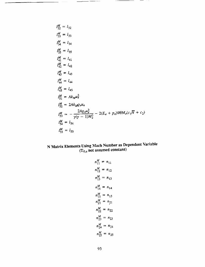
lM= 132

1g = 133

/_4 = /34

3M5 135

l_ = 141

lM = t42

lM__ 14 3

IM = 144

lM_ 145

l M -- AkM u2

l_2 = 2AkMO eu e

2AQ eu2el_ = -

y(?- 1)Me3

IM = 154

1M = 155

- 2(Ee + pe)Ti_OMe(clH + c 2)

N Matrix Elements Using Mach Number as Dependent Variable

(To,e not assumed constant)

tl M = rill

nM -- hi2

tl M = n13

tl M = !114

rl_5 = n15

tl M = rt21

n M = n22

tl M = n23

tl M = t124

n M = //25

93

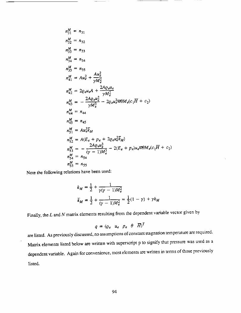
n_l -----n31

nM = ll32

nM = /,133

n3M4 -_ n34

n M = r135

Au_n M = Au 2 + yM"_e

= 2eeu +2Ao eu 2

nM= r,M ,rtM44-" n44

n_5 = n45

aM = AU3_M

2AQeUe

yM2e

2eeu_WOM_(cl_+ c2)

2AQeue3

n M = (y- 1)M 3

n M -- n54

n M = n55

Note the following relations have been used:

---- A(E e -4" Pe q" 2QeU2"kM)

2(Ee + pe)UeiriXOMe(ClH + c 2)

kM.._ l + .1y(y 1)Me2

ll)Me 2 = 1(1 _y) +kM = ½ + (r - _,k.

Finally, the L and N matrix elements resulting from the dependent variable vector given by

q = (Oe Ue Pe 0 _r) T

are listed. As previously discussed, no assumptions of constant stagnation temperature are required.

Matrix elements listed below are written with superscript p to signify that pressure was used as a

dependent variable. Again for convenience, most elements are written in terms of those previously

listed.

94

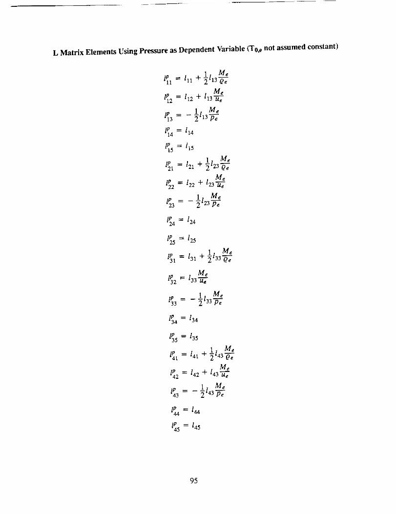
L Matrix Elements Using Pressure as Dependent Variable (To_ not assumed constant)

lP1 = 111 + l ll3Me

Mel_2 - t_2+ l_3

liP3 = -- _113 Me

lP4 114

lP5 115

_-23"bVMe

l_2 = /22 + 123

l_--- _lt Me_'z3 -F;

lP4 = /24

l_5 =125

2 33 _e

lP3 1 t Me= - _-33_',

1 t Me14Pl "" /41 + _'43 _'e

lP2 = /42 + /43

lP3 "- __ 1_.I Me2 "4S _-e

lp --144

95

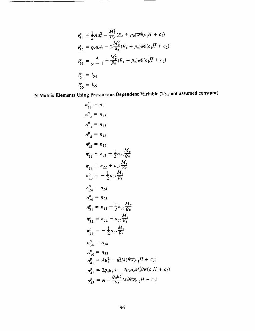
1 2 M2 (Ee q- pe)iJ_O(¢ln" "t- c2)l_l = _Aue - 0-7

lt_2 = OeueA - 2"_e (Ee + pe)iTiTO(clH + c 2)

= a +M_1P53 ), 1 -ff-_e(Ee + pe)i:iTO(clH + c2)

lP4 = /54

155 -- 155

N Matrix Elements Using Pressure as Dependent Variable (To,e not assumed constant)

riP 1 =nll

nP 2 = n12

nPl3 = 1113

riP14 "-- /114

riP5 = hi5

1 Me"_1= "21+ _"23

MenP2 = n22 + n23"_e

nP 3 -ln23 Me=

n_4 = n24

n_5 = n25

1 Men_l = n31 + _n33-0_-- e

Men_2 = n32 + n33--ff_-e

n_3 -ln33 Me= -g-2e

nP 4 = n34

nP 5 ---- n35

nP41 = au 2 - u2M2OW(cxj_ + c 2)

nP 2 = _eUe A -- 2_OeUeM2Ow--(ClF[ + c 2)u 2

':,3= A + _eM_O_(_x-a+ _)

96

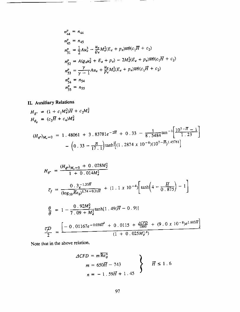
n_l -----rt44

nP5 = n45

i 3 _ _2:_nP551= _Aue Qe,..ev-.e + pe)WO(clF[ + c 2)

nP52 = A(oeU2e + Ee + Pe) - 2M2e(Ee + pe)W---O(cl"H + c2)

= Y Aue + "_eM2e(Ee + pe)TC;O(clH + c 2)n_3 7' - 1

nP 4 = n54

nP 5 "- //55

IL Auxiliary Relations

H3. = (1 + ClM2)H+ c2 M2

HOo = (c3rT + %)M2e

(Ho')M.--O 1 111o7 1]= 1.48061 + 3.83781e -2'7 + 0.33 8.5484 tan ]..23

- O. 33 lff _ 1 tanh (1 . 2874 x 10-6)(107-/7)1'45761

_f "-"

(Ho.)M_ 0 + O. 028M 2

1 + O. O14M 2

0. 3e 1"33/7+

(log 10 R'eo) 1.74 + 0.31/7(1.1x lO-4)[tanh(4

0

g0.92Me 2

1 - 7- .z.z---:-..tanh[1.49(H - 0.9)]13_ +M_

-0.01167e -°'°38//_ + 0.0115 + + (9.0 x lO-8)e 1.60317]

2

Note that in the above relation,

(I + 0.025M 1.4)

ACFD = m Re_ ,)

m = 650H- 743

n = - 1.59H'+ 1.45

H_<l.6

97

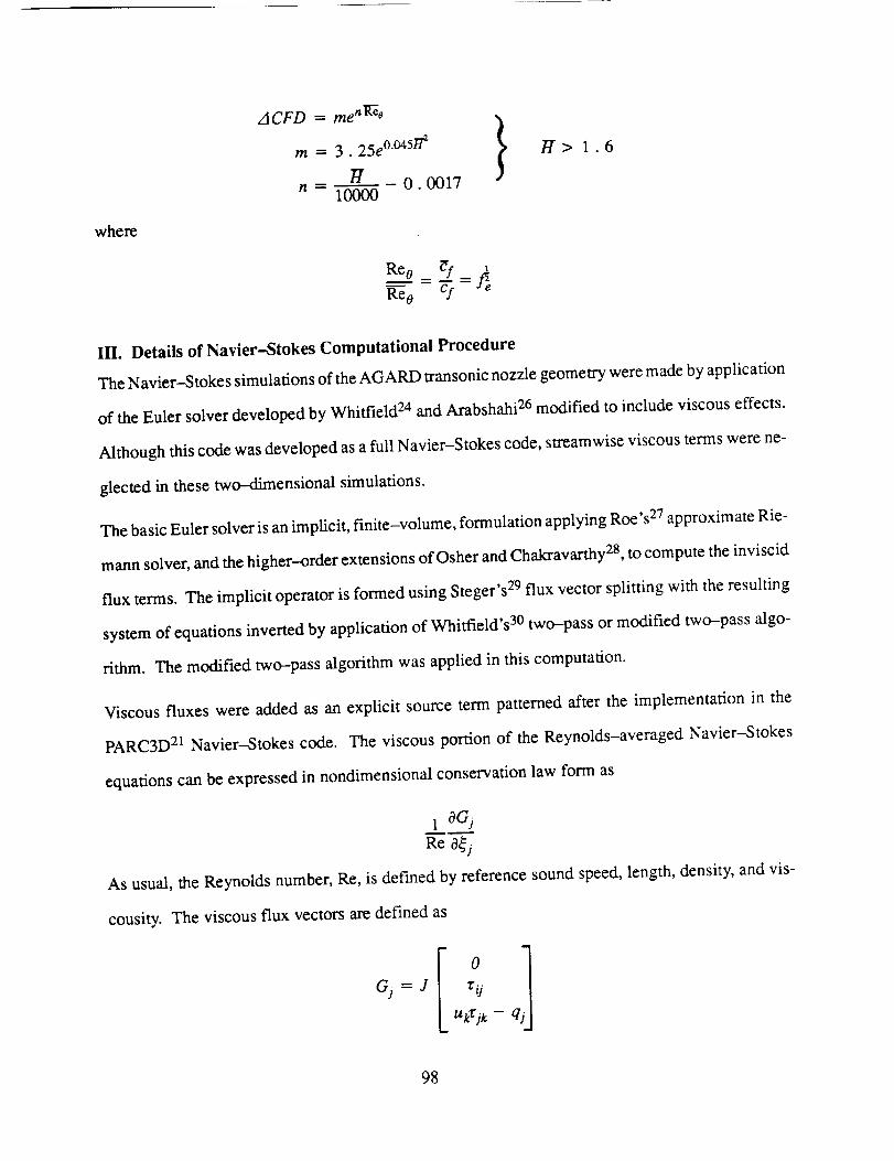
where

ACFD = menlGe

m = 3.25e °'°45_

n - i7" 0.001710000

/7> 1.6

IH. Details of Navier-Stokes Computational Procedure

The Navier-Stokes simulations of the AGARD transonic nozzle geometry were made by application

of the Euler solver developed by Whitfield 24 and Arabshahi 26 modified to include viscous effects.

Although this code was developed as a full Navier--Stokes code, streamwise viscous terms were ne-

glected in these two--dimensional simulations.

The basic Euler solver is an implicit, finite-volume, formulation applying Roe's 27 approximate Rie-

mann solver, and the higher-order extensions of Osher and Chakravarthy 28, to compute the inviscid

flux terms. The implicit operator is formed using Steger's 29 flux vector splitting with the resulting

system of equations inverted by application of Whitfield's 3° two-pass or modified two-pass algo-

rithm. The modified two-pass algorithm was applied in this computation.

Viscous fluxes were added as an explicit source term patterned after the implementation in the

PARC3D 21 Navier-Stokes code. The viscous portion of the Reynolds-averaged Navier-Stokes

equations can be expressed in nondimensional conservation law form as

10Gj

Re O_j

As usual, the Reynolds number, Re, is def'med by reference sound speed, length, density, and vis-

cousity. The viscous flux vectors are defined as

Gj=J[r 0

ukrjk --

98

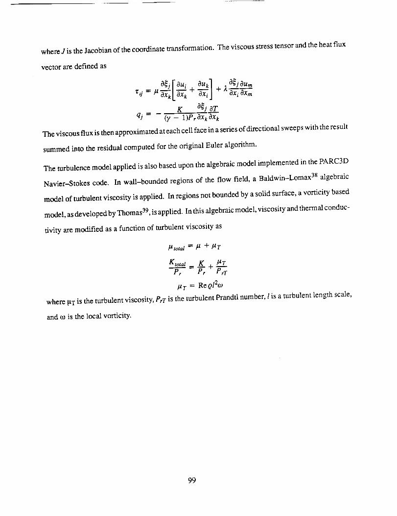
whereJ is the Jacobian of the coordinate transformation. The viscous stress tensor and the heat flux

vector are defined as

rou,o,,,,1 ou,,,Oxi Oxm

K O_j aTqj= - (y - 1)Pr Oxk Oxk

The viscous flux is then approximated at each cell face in a series of directional sweeps with the result

summed into the residual computed for the original Euler algorithm.

The turbulence model applied is also based upon the algebraic model implemented in the PARC3D

Navier---Stokes code. In wall-bounded regions of the flow field, a Baldwin-Lomax 38 algebraic

model of turbulent viscosity is applied. In regions not bounded by a solid surface, a vorticity based

model, as developed by Thomas 39, is applied. In this algebraic model, viscosity and thermal conduc-

tivity are modified as a function of turbulent viscosity as

_ total = k t "1" kiT

Ktot_._....Jt= K_. + ki_..LTPr Pr PrT

kiT = ReQ 12_°

where Wr is the turbulent viscosity, PrT is the turbulent Prandtl number, l is a turbulent length scale,

and 03 is the local vorticity.

99

NOMENCLATURE

a

A

b

Cf

Cv

C

D

e

E

f

F

G

h

H

HOo

HO.

K

L

e#

M

N

Smax

nij

P

Pr

q

r

R

Re

t

T

U

U_

speed of sound

area

right-hand-side vector

skin friction

constant volume specific heat

function used in dissipation model; also used as constant for inflow boundary conditions

dissipation integral

internal energy

total energy

scalar function

vector function

function used in dissipation model; also denotes viscous flux vector

channel half-height

"incompressible" shape factor _'r/0"

shape factor, 6*/0

shape factor, 0o/0

shape factor, 0"/0

thermal conductivity

temporal derivative coefficient matrix

(ij) th element of L matrix

Mach number

spatial derivative coefficient matrix

total number of grid points

(ij) th element of N matrix

pressure

Prandfl number

dependent variable vector, also denotes heat flux vector in Navier-Stokes code

function used in dissipation model

radius; also used to denote perfect gas constant

Reynolds number

time coordinate

temperature

velocity

friction velocity (u 2 = rw/O)

100

x

Y

y+

Y

5"

A

V

0

O*

OQ

k

_t

V

Q

tO

axial coordinate; also used to denote dependent variable in Section III.a

coordinate normal to wall

boundary-layer coordinate (y + =_-_)

ratio of specific heats

displacement thickness

"incompressible" displacement thickness

5"

forward difference operator

backward difference operator

momentum thickness

"incompressible" momentum thickness

energy thickness

density thickness

eigenvalue; also denotes second coefficient of viscosity

absolute viscosity

CFL number

parameter used in grid stretching; also denotes curvilinear coordinate used in Navier-Stokescode

density

shear stress

function used in dissipation model

vorticity

e boundary-layer "edge", or inviscid core value

i axial index

m iteration parameter

max denotes a maximum value

n denotes the n m equation or dependent variable; also denotes time level

ref reference condition

T denotes a turbulent quantity

0 stagnation condition

w wall

oo reference condition

k 0 for planar flow, 1 for axisymmetric

101

M

PA

signifies Mach number used as dependent variable and T0, e _ constant

signifies pressure used as dependent variable and T0, e _ constant

dimensional quantity

102