US000009348956B220160524 - NASA · US 9,348,956 B2 Page 3 (56) References Cited OTHER PUBLICATIONS...

111111111111111111111111111111111111111111111111111111111111111111111111

(12) United States PatentRodriguez et al.

(54) GENERATING A SIMULATED FLUID FLOWOVER A SURFACE USING ANISOTROPICDIFFUSION

(71) Applicant: Aerion Corporation, Reno, CA (US)

(72) Inventors: David L. Rodriguez, Palo Alto, CA(US); Peter Sturdza, Redwood City, CA(US)

(73) Assignee: AERION CORPORATION, Reno, NV(US)

(*) Notice: Subject to any disclaimer, the term of thispatent is extended or adjusted under 35U.S.C. 154(b) by 196 days.

This patent is subject to a terminal dis-claimer.

(21) Appl. No.: 13/887,199

(22) Filed: May 3, 2013

(65) Prior Publication Data

US 2013/0246024 Al Sep. 19, 2013

Related U.S. Application Data

(63) Continuation of application No. 13/046,469, filed onMar. 11, 2011, now Pat. No. 8,437,990.

(51) Int. Cl.G06F 17/10 (2006.01)G06F 17/50 (2006.01)

(52) U.S. Cl.CPC ........ G06F 17/5018 (2013.01); G06F 17/5095

(2013.01); G06F 2217116 (2013.01); G06F2217146 (2013.01)

(58) Field of Classification SearchCPC ............ G06F 17/5095; G06F 17/5018; G06F

2217/46; G06F 2217/16

200

(io) Patent No.: US 9,348,956 B2(45) Date of Patent: *May 24, 2016

USPC .............................................................. 703/2See application file for complete search history.

(56) References Cited

U.S. PATENT DOCUMENTS

5,544,524 A 8/1996 Huyer et al.5,901,928 A 5/1999 Raskob, Jr.6,516,652 131 2/2003 May et al.7,054,768 132 5/2006 Anderson

(Continued)

OTHER PUBLICATIONS

International Search Report and Written Opinion received for PCTPatent Application No. PCT/US2011/067917, mailed on May 1,2012, 10 pages.

(Continued)

Primary Examiner Kamini S ShahAssistant Examiner Russ Guill(74) Attorney, Agent, or Firm Morrison & Foerster LLP

(57) ABSTRACT

A fluid-flow simulation over a computer-generated surface isgenerated using a diffusion technique. The surface is com-prised of a surface mesh of polygons. A boundary-layer fluidproperty is obtained for a subset of the polygons of the surfacemesh. A gradient vector is determined for a selected polygon,the selected polygon belonging to the surface mesh but notone of the subset of polygons. A maximum and minimumdiffusion rate is determined along directions determinedusing the gradient vector corresponding to the selected poly-gon. A diffusion-path vector is defined between a point in theselected polygon and a neighboring point in a neighboringpolygon. An updated fluid property is determined for theselected polygon using a variable diffusion rate, the variablediffusion rate based on the minimum diffusion rate, maxi-mum diffusion rate, and the gradient vector.

20 Claims, 12 Drawing Sheets

202Obtain a Bot.nda,y-;ayer Fluid Property for a S-,bset of Sw race-Mesh Polygons.

20eDeterrrdne a Pressures_ Gradient for a Selected Polygon.

206Definc a F,1ir'umum Diffusion Rate Along the Direction of the Pressure Gradient and aMaxirmlr;o Diffusion Rate Peipcndirular to the Direction of ?hc Pressure Gradient.

208Detine a Dffusio. -Path Vector Between the Selected Surface Aiesh Polygori and A

Neighboring Polygon.

210Determine ,-a Variable Diffusion Rate.

212Determine a Boundary-Layer Fluid Property for the Selected Polygon.

https://ntrs.nasa.gov/search.jsp?R=20160007314 2018-07-13T06:04:32+00:00Z

US 9,348,956 B2


U.S.PATENTDOCUMENTS

7,251,592 B1 7/2007 Praisner et al.8,457,939 B2 6/2013 Rodriguez et al.

2005/0098685 Al 5/2005 Segota et al.2006/0025973 Al 2/2006 Kim2007/0034746 Al 2/2007 Shmilovich et al.2008/0061192 Al 3/2008 Sullivan2008/0163949 Al 7/2008 Duggleby et al.2008/0177511 Al 7/2008 Kamatsuchi2008/0300835 Al 12/2008 Hixon2009/0065631 Al 3/2009 Zha2009/0171596 Al 7/2009 Houston2009/0171633 Al 7/2009 Aparicio Duran et al.2009/0234595 Al 9/2009 Okcay et al.2009/0312990 Al 12/2009 Fouce et al.2010/0036648 Al 2/2010 Mangalam et al.2010/0250205 Al 9/2010 Velazquez Lopez et al.2010/0268517 Al 10/2010 Calmels2010/0276940 Al 11/2010 Khavari et al.2010/0280802 Al 11/2010 Calmels2010/0305925 Al 12/2010 Sendhoff et al.2012/0173219 Al 7/2012 Rodriguez et al.2012/0245903 Al 9/2012 Sturdza et al.

OTHERPUBLICATIONS

International Search Report and Written Opinion received for PCT

Patent Application No. PCT/US2012/030189, mailed on Jun. 20,

2012, 7 pages.International Search Report and Written Opinion received for PCTPatent Application No. PCT/US2012/030427, mailed on Jun. 20,2012, 9 pages.International Search Report and Written Opinion received for PCTPatent Application No. PCT/US2012/028606, mailed on Jun. 1,2012, 11 pages.Non Final Office Action received for U.S. Appl. No. 12/982,744,mailed on Oct. 2, 2012, 9 pages.Notice ofAllowance received for U.S. Appl. No. 13/046,469, mailedon Jan. 10, 2013, 19 pages.Aftosmis et al., "Applications of a Cartesian Mesh Boundary-LayerApproach for Complex Configurations", 44th AIAA Aerospace Sci-ences Meeting, Reno NV, Jan. 9-12, 2006, pp. 1-19.Allison et al., "Static Aeroelastic Predictions for a Transonic Trans-port Model Using an Unstructured-Grid Flow Solver Coupled with aStructural Plate Technique", NASA/TP-2003-2012156, Mar. 2003,49 pages.Balay et al., "PETSc Users Manual", ANL-95/11, Revision 3.1, Mar.2010, pp. 1-189.Bartels et al., "CFL3D Version 6.4-General Usage and AeroelasticAnalysis", NASA/TM-2006-214301, Apr. 2006, 269 pages.Carter, James E., "A New Boundary-Layer Inviscid Iteration Tech-nique for Separated Flow", AIAA 79-1450, 1979, pp. 45-55.Cebeci et al., "VISCID/INVISCID Separated Flows", AFWAL-TR-86-3048, Jul. 1986, 95 pages.Coenen et al., "Quasi-Simultaneous Viscous-Inviscid Interaction forThree-Dimensional Turbulent Wing Flow", ICAS 2000 Congress,2000, pp. 731.1-731.10.Crouch et al., "Transition Prediction for Three-Dimensional Bound-ary Layers in Computational Fluid Dynamics Applications", AIAAJournal, vol. 40, No. 8, Aug. 2002, pp. 1536-1541.Dagenhart, J. Ray, "Amplified Crossflow Disturbances in theLaminar Boundary Layer on Swept Wings with Suction", NASATechnical Paper 1902, Nov. 1981, 91 pages.Drela, Mark, "Two-Dimensional Transonic Aerodynamic Designand Analysis Using the Euler Equations", Ph.D. thesis, Massachu-setts Institute of Technology, Dec. 1985, pp. 1-159.Drela et al., "Viscous-Inviscid Analysis of Transonic and LowReynolds Number Airfoils", AIAA Journal, vol. 25, No. 10, Oct.1987, pp. 1347-1355.Drela, Mark, "XFOIL: An Analysis and Design System for LowReynolds Number Airfoils", Proceedings of the Conference on LowReynolds Number Aerodynamics, 1989, pp. 1-12.

Drela, Mark, "Implicit Implementation of the Full en TransitionCriterion", 21st Applied Aerodynamics Conference, AIAA Paper2003-4066, Jun. 23-26, 2003, pp. 1-8.Eymard et al., "Discretization Schemes for Heterogeneous andAnisotropic Diffusion Problems on General NonconformingMeshes", Available online as HAL report 00203269, Jan. 22, 2008,pp. 1-28.Frink et al., "An Unstructured-Grid Software System for SolvingComplex Aerodynamic Problems", NASA/95-28743, 1995, pp. 289-308.Fuller et al., "Neural Network Estimation of Disturbance GrowthUsing a Linear Stability Numerical Model", American Institute ofAeronautics and Astronautics, Inc., Jan. 6-9, 1997, pp. 1-9.Gaster, M., "Rapid Estimation of N-Factors for Transition Predic-tion", 13th Australasian Fluid Mechanics Conference, Dec. 13-18,1998, pp. 841-844.Gleyzes et al., "A Calculation Method of Leading-Edge SeparationBubbles", Chapter 8, Numerical and Physical Aspects of Aerody-namic Flows II, 1984, pp. 173-192.Hess et al., "Calculation of Potential Flow About Arbitrary Bodies",Progress in Aerospace Sciences, 1967, pp. 1-138.Jespersen et al., "Recent Enhancements to OVERFLOW", AIAA97-0644, 1997, pp. 1-17.Krumbein, Andreas, "Automatic Transition Prediction and Applica-tion to Three-Dimensional Wing Configurations", Journal of Air-craft, vol. 44, No. 1, Jan.-Feb. 2007, pp. 119-133.Langlois et al., "Automated Method for Transition Prediction onWings in Transonic Flows", Journal of Aircraft, vol. 39, No. 3,May-Jun. 2002, pp. 460-468.Lewis, R. L, "Vortex Element Methods for Fluid Dynamic Analysisof Engineering Systems", Cambridge University Press, 2005, 12pages.Lock et al., "Viscous-Inviscid Interactions in External Aerodynam-ics", Progress in Aerospace Sciences, vol. 24, 1987, pp. 51-171.Mavriplis, Dimitri J., "Aerodynamic Drag Prediction Using Unstruc-tured Mesh Solvers", National Institute of Aerospace, 2003, pp. 1-83.Perraud et al., "Automatic Transition Predictions Using SimplifiedMethods", AIAA Journal, vol. 47, No. 11, Nov. 2009, pp. 2676-2684.Potsdam, Mark A., "An Unstructured Mesh Euler and InteractiveBoundary Layer Method for Complex Configurations", AIAA-94-1844, 12th Applied Aerodynamics Conference, Jun. 20-23, 1994, pp.1-8.Rasmussen et al., "Gaussian Processes for Machine Learning", MITPress, 2006, 266 pages.Rodriguez et al., "A Rapid, Robust, andAccurate Coupled Boundary-Layer Method for Cart3d", American Institute of Aeronautics andAstronautics, 2012, pp. 1-19.Rodriguez et al., "Improving the Accuracy of Euler/Boundary-LayerSolvers with Anisotropic Diffusion Methods", American Institute ofAeronautics and Astronautics, 2012, pp. 1-15.Smith et al., "Interpolation and Gridding of Aliased GeophysicalData Using Constrained Anisotropic Diffusion to Enhance Trends",SEG International Exposition and 74th Annual Meeting, Oct. 10-15,2004, 4 pages.Spreiter et al., "Thin Airfoil Theory Based on Approximate Solutionof the Transonic Flow Equation", Report 1359 National AdvisoryCommittee for Aeronautics, 1957, pp. 509-545.Stock et al., "A Simplified en Method for Transition Prediction inTwo-Dimensional, Incompressible Boundary Layers", Journal ofFlight Sciences and Space Research, vol. 13, 1989, pp. 16-30.Sturdza, Peter, "An Aerodynamic Design Method for SupersonicNatural Laminar Flow Aircraft", Stanford University Dec. 2003, 198pages.Veldman, A. E. P., "New, Quasi-Simultaneous Method to CalculateInteracting Boundary Layers", AIAA Journal, vol. 19, No. 1, Jan.1981, pp. 79-85.Veldman et al., "The Inclusion of Streamline Curvature in a Quasi-Simultaneous Viscous-Inviscid Interaction Method for TransonicAirfoil Flow", Department of Mathematics, University ofGroningen, Nov. 10, 1998, pp. 1-18.Veldman, Arthur E. P:, "A Simple Interaction Law for Viscous-Inviscid Interaction", Journal of Engineering Mathematics, vol. 65,Aug. 14, 2009, pp. 367-383.

US 9,348,956 B2


OTHER PUBLICATIONS

Veldman, Arthur E. P., "Quasi-Simultaneous Viscous-Inviscid Inter-action for Transonic Airfoil Flow", American Institute ofAeronauticsand Astronautics Paper 2005-4801, 4th Theoretical Fluid MechanicsMeeting, Jun. 6-9, 2005, pp. 1-13.Veldman, Arthur E. P., "Strong Viscous-Inviscid Interaction and theEffects of Streamline Curvature", CWI Quarterly, vol. 10, No. 3&4,1997, pp. 353-359.Washburn, Anthony, "Drag Reduction Status and Plans LaminarFlow and AFC', AIAA-Aero Sciences Meeting, Jan. 4-7, 2011, pp.1-25.Weickert et al., "Tensor Field Interpolation with PDEs", Universitatdes Saarlandes, 2005, 17 pages.Notice ofAllowance received for U.S. Appl. No. 13/069,374, mailedon May 15, 2013, 23 pages.Davis et al., "Control of Aerodynamic Flow", AFRL-VA-WP-TR-2005-3130, Delivery Order 0051: Transition Prediction MethodReview Summary for the Rapid Assessment Tool for Transition Pre-diction (RATTraP), Jun. 2005, 95 pages.Herbert, Thorwald, "Parabolized Stability Equations", AnnualReview of Fluid Mechanics, vol. 29, 1997, pp. 245-283.Jones et al., "Direct Numerical Simulations of Forced and UnforcedSeparation Bubbles on an Airfoil at Incidence", Journal of FluidMechanics, vol. 602, 2008, pp. 175-207.Khorrami et al., "Linear and Nonlinear Evolution of Disturbances inSupersonic Streamwise Vortices", High Technology Corporation,1997, 87 pages.

Matsumura, Shin, "Streamwise Vortex Instability and HypersonicBoundary Layer Transition on the Hyper 2000", Purdue University,Aug. 2003, 173 pages.Tsao et al., "Application of Triple Deck Theory to the Prediction ofGlaze Ice Roughness Formation on an Airfoil Leading Edge", Com-puters & Fluids, vol. 31, 2002, pp. 977-1014.International Preliminary Report on Patentability received for PCTPatent Application No. PCT/US2011/067917, mailed on Jul. 11,2013, 9 pages.International Preliminary Report on Patentability received for PCTPatent Application No. PCT/US2012/028606, mailed on Sep. 26,2013, 10 pages.International Preliminary Report on Patentability received for PCTPatent Application No. PCT/US2012/030427, mailed on Apr. 3,2014, 8 pages.International Preliminary Report on Patentability received for PCTPatent Application No. PCT/US2 0 1 2/03 0 1 89, mailed on Mar. 27,2014, 6 pages.Final Office Action Received for U.S. Appl. No. 13/070,384, mailedon Apr. 11, 2014, 6 pages.Non Final Office Action received for U.S. Appl. No. 13/070,384,mailed on Jan. 6, 2014, 7 pages.Non-Final Office Action received for U.S. Appl. No. 13/887,189,mailed on Apr. 10, 2014, 6 pages.Notice ofAllowance received for U.S. Appl. No. 13/070,384, mailedon Jul. 18, 2014, 8 pages.Notice ofAllowance received for U.S. Appl. No. 13/887,189, mailedon Sep. 4, 2014, 9 pages.

U.S. Patent May 24, 2016 Sheet 1 of 12 US 9,348,956 B2

200

202

Obta

in a Boundary-

layer Fl

uid Pr

oper

ty for a Subset of Su

rfac

e-Mesh Polygons.

204

Dete

rmin

e a Pre

ssur

e Gr

adie

nt for

a Selected Po

lygo

n.

2061

Define a Mln

in'l

Urn Di

ffus

ion Fa

te Alo

ng the

Direction of th

e Pr

essu

re Gra

dien

t and a

Maximum Diffusion Pate Perpendicular to the Di

rect

ion of the Pre

ssur

e Gr

adie

nt.

208

Define a Diffusion-P

ath 'hector Between the Sel

ecte

d Surface Mesh Pol

ygon

and A

Neighboring Polygon.

210

Dete

rmin

e a Variable Di

ffus

ion Da

te.

212

Determine a Boundary-La

yer Fl

uid Pr

oper

ty for the Selected Po

lygon.


Kt r_,

Cpl t~ Cri~U


IqCD


c~co


a

et~e4-


m


.10

------

------

------

------

------

------

------

------

------

------

------

------

------

------

------

------

------

------

------

------

------

------

------

------

------

------

------

------

------

------

------

------

------

------

------

------

------

------

------

------

------

------

------

------

------

----

1102

1110

1112

1114

Processor

RAM

Hard Dri

ve

Storage Media

1104

1108

1108

Data Input

Data Output

User

Disp

lay

1100


C)

ME

US 9,348,956 B2

GENERATING A SIMULATED FLUID FLOWOVER A SURFACE USING ANISOTROPIC

DIFFUSION

CROSS REFERENCE TO RELATED 5

APPLICATIONS

The present application is a continuation of U.S. applica-tion Ser. No. 13/046,469, filed Mar. 11, 2011, which is incor-porated herein by reference in its entirety. 10

STATEMENT REGARDING FEDERALLYSPONSORED RESEARCH OR DEVELOPMENT

This invention was made with Government support under 15contract NN08AA08C awarded by NASA. The Governmenthas certain rights in the invention.

BACKGROUND 20

1. FieldThis application relates generally to simulating a fluid flow

over a computer-generated surface and, more specifically, toestimating a viscous fluid property distribution over a com- 25puter-generated surface using an anisotropic diffusion tech-nique.

2. Description of the Related ArtAerodynamic analysis of an aircraft moving through a fluid

typically requires an accurate prediction of the properties of 30the fluid surrounding the aircraft. Accurate aerodynamicanalysis is particularly important when designing aircraftsurfaces, such as the surface of a wing or control surface.Typically, the outer surface of a portion of the aircraft, such asthe surface of a wing, is modeled, either physically or by 35computer model, so that a simulation of the fluid flow can beperformed and properties of the simulated fluid flow can bemeasured. Fluid-flow properties are used to predict the char-acteristics of the wing including lift, drag, boundary-layervelocity profiles, and pressure distribution. The flow proper- 40ties may also be used to map laminar and turbulent flowregions near the surface of the wing and to predict the forma-tion of shock waves in transonic and supersonic flow.A computer-generated simulation can be performed on a

computer-generated aircraft surface to simulate the fluid 45dynamics of a surrounding fluid flow. The geometry of thecomputer-generated aircraft surface is relatively easy tochange and allows for optimization through design iterationor analysis of multiple design alternatives. A computer-gen-crated simulation can also be used to study situations that may 50be difficult to reproduce using a physical model, such assupersonic flight conditions. A computer-generated simula-tion also allows a designer to measure or predict fluid-flowproperties at virtually any point in the model by direct query,without the difficulties associated with physical instrumenta- 55tion or data acquisition techniques.

In some cases, a computer-generated simulation includes acomputational fluid dynamics (CFD) simulation module usedto predict the properties of the fluid flow. A CFD simulationmodule estimates the properties of a simulated fluid flow by 60applying an algorithm or field equation that estimates theinteraction between small simulated fluid volumes, alsoreferred to as fluid cells. Because a single CFD simulationmodule may include millions of individual fluid cells, thecomplexity of the relationship between fluid cells can have a 65large effect on the computational efficiency of the simulation.Complex CFD simulation modules can be computationally

2expensive and require hours or even days to execute usinghigh-performance computer processing hardware.To reduce the computational burden, in some instances it is

desirable to use a CFD simulation module that simplifies thefluid dynamics and produces a fluid simulation that can besolved more rapidly. For example, for fluid flows that arerelatively uniform or are located away from an aircraft sur-face, a simplified simulationthat minimizes or ignores certainfluid dynamic phenomena can be used. In the examples dis-cussed below, a simplified simulation may ignore fluiddynamic contributions due to fluid viscosity, which, in somecases, have little effect on the overall behavior of the fluid. Byusing a simplified simulation, processing time may beimproved.In other situations, where the fluid flow is not as uniform, it

may be necessary to use a CFD simulation module that ismore sophisticated and capable of accurately predicting thefluid properties, using more complex fluid dynamics. In theexamples discussed below, a more sophisticated simulationmay account for dynamic contributions due to fluid viscosity.Under certain conditions, the more sophisticated simulationmay be more accurate, particularly for portions of the fluidflow where fluid viscosity affects the results. However, moresophisticated simulation modules are also likely to requiremore computing resources, and therefore may require moretime to solve.

SUMMARY

One exemplary embodiment includes a computer-imple-mented method of generating a fluid-flow simulation over acomputer-generated surface. The surface is comprised of asurface mesh of polygons. A boundary-layer fluid property isobtained for a subset of the polygons of the surface mesh ofpolygons. The subset represents a portion of the computer-generated surface. A pressure-gradient vector is determinedfor a selected polygon, the selected polygon belonging to thesurface mesh of polygons but not one of the subset of poly-gons for which a boundary-layer fluid property has beenobtained. A minimum diffusion rate is defined along thedirection of the pressure gradient vector of the selected poly-gon. A maximum diffusion rate is also defined in a directionperpendicular to the direction of the pressure gradient vectorof the selected polygon. A diffusion-path vector is definedbetween a point in the selected polygon and a neighboringpoint in a neighboring polygon, the neighboring polygonbelonging to the subset of polygons for which a boundary-layer fluid property has been obtained. An updated fluid prop-erty is determined for the selected polygon using a variablediffusion rate, the variable diffusion rate based on the mini-mum diffusion rate, maximum diffusion rate, and angulardifference between the diffusion-path vector and the pressuregradient vector.

DESCRIPTION OF THE FIGURES

FIG.1 depicts a computer-generated fluid flow applied to acomputer-generated aircraft surface.FIG. 2 depicts an exemplary process for propagating a

boundary-layer fluid property over a computer-generated air-craft surface using anisotropic diffusion.FIG. 3 depicts an exemplary surface mesh and fluid-flow

mesh for simulating a fluid flow over a computer-generatedwing surface.FIG. 4 depicts a surface mesh of polygons representing a

wing surface and strip areas representing a portion of wingsurface.

US 9,348,956 B23

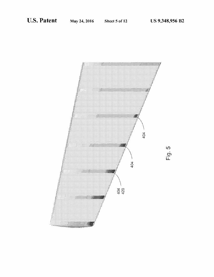
FIG. 5 depicts results of a boundary-layer CFD simulationperformed only for strip areas of a wing surface.

FIG. 6 depicts exemplary diffusion paths on a surface meshof polygons representing a computer-generated wing surface.FIGS. 7a and 7b depict an exemplary fluid flow around a

wing surface.FIG. 8 depicts an exemplary pressure distribution over a

computer-generated wing surface using isotropic diffusionand a finite-volume solver.

FIG. 9 depicts an exemplary pressure distribution over acomputer-generated wing surface using an inviscid CFDsimulation module.

FIG. 10 depicts exemplary pressure distribution over acomputer-generated wing surface using anisotropic diffusionand a finite-volume solver.

FIG. 11 depicts an exemplary computer system for simu-lating a fluid flow over a computer-generated aircraft surface.

FIG. 12 depicts an exemplary computer network.The figures depict one embodiment of the present inven-

tion for purpo ses of illustration only. One skilled in the art willreadily recognize from the following discussion that alterna-tive embodiments of the structures and methods illustratedherein can be employed without departing from the principlesof the invention described herein.

DETAILED DESCRIPTION

As discussed above, a computer-generated simulation canbe used to analyze the aerodynamic performance of a pro-posed aircraft surface, such as a wing or control surface.Using known geometry modeling techniques, a computer-generated aircraft surface that represents the outside surfaceof the proposed aircraft can be constructed. FIG.1 depicts anexemplary computer-generated aircraft surface of the SpaceShuttle orbiter vehicle, external tank, and twin solid-fuelrocket boosters. A CFD simulation module has been appliedusing the computer-generated aircraft surface of the SpaceShuttle orbiter to predict the fluid properties of an exemplaryfluid flow.As shown in FIG. 1, the results of the simulation can be

visually represented as shaded regions on the computer-gen-erated aircraft surface of the Space Shuttle. Different shadesrepresent the predicted pressure distribution resulting fromthe simulated fluid flow. In FIG. 1, transitions between theshaded regions represent locations of predicted pressurechange across the surface of the Space Shuttle. Similarly,different pressures in the surrounding fluid flow are repre-sented as differently shaded regions.

In FIG. 1, the simulation of the fluid flow is visualized bydepicting the predicted pressure distribution. However, thesimulation may be visualized using other fluid properties,including surface velocity, air temperature, air density, andothers. Additionally, the simulation may be used to visualizelocations of developing shock waves or transitions betweenlaminar and turbulent flow.

The simulation allows the designer or engineer to evaluatethe performance of the aircraft geometry for various flowconditions. If necessary, changes can be made to the aircraftgeometry to optimize performance or eliminate an unwantedaerodynamic characteristic. Another simulation can be per-formed using the modified geometry, and the results can becompared. To allow for multiple design iterations, it is advan-tageous to perform multiple simulations in a short amount oftime. However, as described above, there is a trade-offbetween speed and accuracy of the simulation depending onthe type of CFD simulation module used.

_►,

As mentioned above, a computer-generated simulationtypically represents a fluid flow as a three-dimensional fluid-flow mesh of small volumes of fluid called fluid cells. Theshape of the fluid cells can vary depending on the type of

5 fluid-flow mesh used. A CFD simulation module predicts thefluidic interactions between the fluid cells in the fluid-flowmesh, using a fundamental algorithm or field equation.The speed and accuracy of a CFD simulation module

depends, in part, on the field equation used to predict theio interaction between the fluid cells. In some instances, the field

equation simplifies the relationship between fluid cells byignoring or minimizing certain dynamic contributions. Thesefield equations are typically less complex, and therefore aremore computationally efficient. For instance, a simplified

15 algorithm called the Euler method may be used to simulate afluid flow when viscous effects can be minimized or ignored.Viscous effects of a fluid can be ignored when, for example,there is not a significant velocity difference between adjacentfluid cells, and therefore shear forces due to internal friction

20 or viscosity are minimal. A CFD simulation module thatignores or minimizes effects of fluid viscosity can also bereferred to as an inviscid simulation.

In other instances, a more complex field equation is used tomore accurately predict the interaction between the fluid

25 cells. For example, a Navier-Stokes method can be used tosimulate the pressure and shear forces on the fluid cells.Unlike the Euler method mentioned above, the Navier-Stokesmethod accounts for the effects of viscosity and offers a moreaccurate simulation of a fluid flow. A simulated fluid flow that

so accounts for effects due to fluid viscosity can also be referredto as a viscous simulation.

However, the improved accuracy of the Navier-Stokesmethod comes at the cost of increased computational load,and therefore the Navier-Stokes method is generally slower to

35 compute than an Euler-based algorithm. In addition, aNavier-Stokes method may require more (smaller) fluid cellsto generate acceptable results, further increasing the compu-tational load. Thus, selecting the field equation for a CFDmodule often involves a trade-off between speed and accu-

4o racy. In practice, designers may use faster Euler-based CFDmodels to evaluate multiple design iterations and then vali-date the final design iteration with a more accurate Navier-Stokes-based CFD model. However, if the Navier-StokesCFD simulation reveals a design problem, the entire process

45 must be repeated, wasting valuable time and computingresources.The techniques described below are computer-generated

simulations that use both viscous and inviscid field equationsto achieve acceptable accuracy without requiring the compu-

50 tational burden of a full viscous CFD simulation (e.g., aNavier-Stokes-based CFD simulation). In many simulations,there is a region of the fluid flow that can be accuratelypredicted without taking viscous contributions into account.For example, regions of the fluid flow that are located away

55 from an aircraft or wing surface have a relatively uniformvelocity profile. Therefore, an inviscid simulation using, forexample, an Euler-based analysis, can be used to accuratelypredict the behavior of the fluid-flow region. In other fluid-flow regions where there is a less uniform velocity profile, a

60 more complex, viscous simulation can be used.In fluid-flow regions where a viscous simulation is desired,

further computational gains can be realizedby performing theviscous simulation for only a portion of the fluid-flow region.For example, a portion of a boundary-layer fluid-flow region

65 (near a wing surface) may be represented by one or more stripareas. See, for example FIG. 4, depicting strip areas 404extending along the chord direction of the wing and spaced at

US 9,348,956 B25

intervals along the span of the wing. In FIG. 4, the strip areas404 are spaced at regular intervals; however, it is not neces-

sary that they be so. The viscous simulation is performed only

for the strip-area portions of the boundary-layer fluid-flowregion, thereby reducing the number of simulation calcula-tions. As a result, the boundary-layer fluid properties are onlyknown for strip-area portions of the boundary-layer fluid-flow region.

Using the techniques described below, the predictedboundary-layer fluid properties for a portion of a boundary-layer region (represented by, for example, strip areas 404) canbe extended to the other portions of the boundary-layerregion. Specifically, a diffusion technique can be used topropagate a predicted boundary-layer fluid property for thestrip areas 404 to other areas of the computer-generated air-craft surface, between the strip areas 404. In this way, thetechniques described herein may provide an accurate predic-tion of the fluid properties of an entire fluid-flow regionwithout having to perform a CFD simulation for the entireboundary-layer fluid-flow region.1. Exemplary Process for Propagating a Fluid Property UsingDiffusion TechniquesFIG. 2 depicts an exemplary process 200 for propagating

the results of a boundary-layer CFD simulation module for acomputer-generated aircraft surface. The results of theboundary-layer CFD simulation module include one or moreboundary-layer fluid properties (e.g., pressure, temperature,surface velocity, boundary-layer thickness). For purposes ofthis discussion, a computer-generated wing surface is used.However, the technique can be applied to nearly any type ofcomputer-generated aircraft surface, including a computer-generated surface for an aircraft fuselage, nacelle, shroud, orother structure.The exemplary process 200 uses a diffusion technique to

propagate a fluid property over the computer-generated air-craft surface. The term diffusion, as it is used below, relates toa technique for estimating fluid property values over a com-puter-generated surface using fluid property values that are(initially) known for only a portion of the computer-generatedsurface. The estimation is based, in part, on a modified ver-sion of the heat equation, which is also referred to herein as adiffusion equation. Traditionally, a diffusion equation can beused to predict heat diffusion or conduction through a mass orbody of material. However, rather than predict the physicaldiffusion of heat energy, the exemplary process 200 uses adiffusion equation to propagate or distribute fluid propertyvalues from one portion of a computer-generated surface(where the fluid properties are known) to other portions of thecomputer-generated surface (where the fluid properties arenot known).An exemplary two-dimensional, isotropic diffusion equa-

tion that can be used to diffuse a fluid property a over adistance x and y can be expressed as:

6u 62u 62u Equation 1

6t — 6x2 + 37~'

where a is a positive constant representing the diffusion rateand t is time. The diffusion rate a (also called a conductionconstant) determines the rate of diffusion over a given dis-tance, also called a diffusion path. As applied in the exem-plary process 200 below, a diffusion path is typically definedbetween two points on a computer-generated aircraft surface:a first point having an unknown fluid property value and asecond point with a known fluid property value. In general, a

Tlarge diffusion rate tends to produce a more uniform fluid-property distribution between the two points along a diffusionpath. That is, the unknown fluid property value at the firstpoint will be closer to the known fluid property value at the

s second point. Conversely, a small diffusion rate tends to pro-duce a less uniform fluid-property distribution between twopoints along a diffusion path.

Typically, process 200 is performed as part of a computer-generated simulation for a computer-generated aircraft sur-

io face. As mentioned above and discussed in more detail belowwith respect to FIGS. 7a and 7b, a computer-generated simu-lation can be performed using two CFD simulation modules.In the exemplary process 200, an inviscid CFD simulationmodule is used to predict the fluid properties for an inviscid

15 fluid-flow region and a viscous or boundary-layer CFD simu-lation module is used to predict the fluid properties of aviscous fluid-flow region.As shown in FIG. 3, the inviscid fluid-flow region may be

discretized using a fluid-flow mesh 302. In the following20 example, fluid-flow mesh 302 represents the inviscid fluid-

flow region using a three-dimensional array of fluid cells,each fluid cell associated with one or more inviscid-fluidproperties. As explained in more detail below, an inviscidCFD simulation module (using, for example, field equation

25 13, below) can be used to determine inviscid-fluid propertiesfor each fluid cell of the fluid-flow mesh 302.

FIG. 3 also depicts a computer-generated aircraft surface,specifically a wing surface, discretized using a surface meshof polygons 304. While FIG. 3 depicts a surface mesh of

30 triangular polygons, other types of polygons can also be used.FIG. 3 also depicts an exemplary strip area 404 and subset ofpolygons 420, discussed in more detail below with respect toFIGS. 4, 5, and 6.The boundary-layer fluid-flow region is discretized using a

35 two-dimensional array of points within the surface mesh ofpolygons 304. As shown in FIG. 3, the boundary-layer regionmay be represented using boundary-layer prediction points306 located on the computer-generated surface. In thisexample, each boundary-layer prediction point 306 corre-

40 sponds to a polygon in the surface mesh of polygons 304. Theboundary-layer prediction points 306 can be located virtuallyanywhere with respect to a corresponding polygon. However,for ease of explanation, the boundary-layer prediction points306 are depicted as being located near the centroid of each

45 corresponding polygon. While the computer-generated wingsurface is a three-dimensional representation, the surfacemesh of polygons 304 and corresponding boundary-layerprediction points 306 can be treated as a two-dimensionalspace projected onto the three-dimensional computer-gener-

5o ated wing surface. That is, each polygon or boundary-layerprediction point 306 can be identified and located withrespect to the computer-generated wing surface using twocoordinate values (x and y).

Discussed in more detail below with respect to equation 2,55 FIG. 3 also depicts exemplary selected polygon 630 and a set

of fluid cells 320, close in proximity to selected polygon 630.The following operations can be performed as an exem-

plary process 200 for diffusing a boundary-layer propertyover a computer-generated surface. In operation 202, a

6o boundary-layer fluid property for a subset of polygons isobtained. As shown in FIG. 4, the subset of polygons 420 maybe defined as the surface-mesh polygons within a strip area404. For simulations using a computer-generated wing sur-face, as shown in FIG. 5, the strip areas 404 may extend along

65 the chord direction or stream-wise across the computer-gen-erated wing surface. Also shown in FIG. 5, multiple stripareas 404 may be spaced at a regular distance along the span

US 9,348,956 B27

of the wing. In alternative arrangements, the strip areas 404can be oriented along different directions and placed at vari-

ous locations along the computer-generated wing surface.

In this example, a strip area 404 is used to define the subset

of polygons 420. However, other shapes or techniques can be

used to select the subset of polygons 420, as long as thenumber of polygons in the subset of polygons 420 is fewer

than the number of polygons in the surface mesh of polygons

304. For example, the subset of polygons 420 may be definedas those polygons located within a radial distance of a point

on the computer-generated aircraft surface. In anotherexample, the subset of polygons 420 may be one polygon.

To reduce the number of simulation calculations, theboundary-layer simulation is only performed for boundary-

layer prediction points 306 associated with the subset of

polygons 420. Using the example shown in FIG. 4, the bound-ary-layer simulation is performed for each boundary-layer

prediction point 306 associated with a polygon of the subset

of polygons 420 (e.g., polygons within strip areas 404). Note,a boundary-layer simulation is not performed for boundary-

layer prediction points 306 associated with polygons that arenot part of the subset of polygons 420 (e.g., polygons between

strip areas 404).

As explained in more detail below with respect to FIGS. 7a

and 7b, a boundary-layer CFD simulation (using, for

example, field equations 14 and 15, below) can be used todetermine a boundary-layer fluid property for each boundary-

layer prediction point 306 associated with a polygon of the

subset of polygons.

FIG. 5 depicts exemplary results of operation 202. That is,

FIG. 5 depicts the results of a boundary-layer CFD simulation

performed only for a subset of polygons 420 (within strip

areas 404). The shaded areas in FIG. 5 represent the portions

of the boundary-layer fluid-flow region where the boundary-

layer fluid properties are known. Changes in the degree of

shading represent variations in the boundary-layer fluid prop-

erty values. Note that the grey regions (between strip areas

404) represent portions of the boundary-layer fluid-flow

region where the boundary-layer fluid properties are not

known.

In operation 204, a pressure gradient vector Op is deter-

mined for a selected polygon. In the examples shown in FIGS.

3 and 6, the selected polygon 630 is a polygon of the surfacemesh of polygons 304 but is not one of the subset of polygons

420. The direction component of pressure gradient vector Opindicates the direction of greatest pressure change withrespect to the fluid flow near the selected polygon 630.

The pressure gradient Op can be determined using theinviscid fluid-properties of the fluid-flow mesh 302. Asexplained above, an inviscid CFD simulation module can beused to predict the inviscid fluid properties of fluid cells in thefluid-flow mesh 302. Typically, the inviscid fluid propertiesare known for at least the fluid cells (of the fluid-flow mesh302) that are close in proximity to the computer-generatedaircraft surface used for the simulation (e.g., the computer-generated wing surface). In contrast, as mentioned above, theboundary-layer fluid properties are (initially) only known forthe subset of polygons 420 within strip area 404.

Changes in the inviscid fluid pressure can be indicative ofchanges in the boundary-layer fluid properties. Therefore, an

8inviscid pressure gradient vector can be used as a suitableproxy for the gradient of the boundary-layer property being

diffused.

5 In one example, the pressure gradient vector Op is deter-

mined by identifying a set of fluid cells 320 of the fluid-flowmesh 302 that are close in proximity to the selected polygon

630. (See FIG. 3.) Generally, a two-dimensional pressure

gradient vector in an x-y space can be defined as:

10

6p

'

6p

)'

Equation 2

6x 6y~p

—~

15 where p is the pressure of the inviscid fluid flow near the

surface of the wing (represented by the identified set of fluidcells 320 close in proximity to the selected polygon 630).Because the wing is a three-dimensional shape, the proximate

20 inviscid fluid flow represented by the identified set of fluidcells 320 will also be three-dimensional. However, for thesake of simplicity, an inviscid fluid pressure distribution cor-responding to the identified set of fluid cells 320 can betreated as a two-dimensional distribution mapped to the com-

25 puter-generated aircraft surface. Because, in many cases, theinviscid fluid pressure distribution is different for differentareas of the computer-generated aircraft surface, a pressuregradient should be determined for each selected polygonwithin the surface mesh of polygons.

30 As explained in more detail below with respect to opera-

tions 206 and 212, the pressure gradient vector Op is used todetermine the primary and secondary diffusion directions.

For example, the direction of the pressure gradient vector Op35 may be used as the first primary direction di. The direction

perpendicular to the pressure gradient vector Op may be usedas the second primary direction dz.

In operation 206, maximum and minimum diffusion ratesare defined (am_, am,,,, respectively). As discussed above,

40 the diffusion rate determines, in part, the amount of diffusionalong a diffusion path. In this example, a minimum diffusionrate am, is selected for diffusion paths along the first primary

direction d, (the direction of the pressure gradient vector Op).45 A maximum diffusion rate am,,is selected for diffusion paths

along the second primary direction dz (the direction perpen-

dicular to the direction of the pressure gradient vector Op). Insome cases, the maximum diffusion rate am,, is 1,000 to1,000,000 times the minimum diffusion rate am,,,.

50In some cases, when the pressure gradient vector Op is

small or nearly zero, a single diffusion rate can be used. If thediffusion rate is equal or nearly equal in all directions, themaximum and minimum diffusion rates (amp, am,) may be

55 treated as equal, or one of the diffusion rates (amp) can beused as the sole diffusion rate. For example, as discussed inmore detail below with respect to equation 9, when the pres-

sure gradient vector Op is small or nearly zero, the diffusionrate does not depend on direction, and isotropic diffusion can

60 be applied using the maximum diffusion rate (amp).

In operation 208, a diffusion path vector S is definedbetween the selected polygon and a neighboring polygon.The neighboring polygon may or may not be immediately

65 adjacent to the selected polygon. FIG. 6 depicts an exemplaryselected polygon 630 and neighboring polygon 620. The dif-

fusion path vector 640 S between the selected polygon 630

US 9,348,956 B29

and neighboring polygon 620 can be defined as a vectorbetween the respective boundary-layer prediction points 306of the selected polygon 630 and neighboring polygon 620.

The direction ddf eof the diffusion path vector 640 S can beexpressed as an angle from horizontal.

In FIG. 6, the selected polygon 630 is a polygon outside ofthe strip area 404. Therefore, selected polygon 630 is not oneof the subset of polygons for which a boundary-layer fluidproperty is known. In this example, neighboring polygon 620is inside of the strip area 404, and therefore is one of the subsetof polygons 420 for which a boundary-layer fluid property is

known. Thus, in this example, the diffusion path vector 640 Sdefines a path from a portion of the boundary-layer fluid-flowregion where the fluid properties are known to a portion of theboundary layer fluid-flow region where the fluid propertiesare not known.

Other diffusion paths are also possible. For example, FIG.6 depicts an alternative selected polygon 631 and alternativeneighboring polygon 621. Here, both the selected polygon631 and neighboring polygon 621 are outside of the strip area

404. The diffusion path vector 641 _J defines a path betweentwo portions of the boundary layer fluid-flow region wherethe fluid properties are unknown.

In operation 210, a variable diffusion rate a is determined.The variable diffusion rate a depends on the direction dd fse

of the diffusion path vector S, the maximum diffusion rateam_, minimum diffusion rate am,,,, and first primary direc-tion di . As explained above, the minimum diffusion rate am,applies to diffusion along the first primary direction d, (the

direction of the pressure gradient vector Op). The maximumdiffusion rate am,, applies to diffusion along a second pri-mary direction dz (the direction perpendicular to the direction

of the pressure gradient vector Op). For diffusion in directionsother than the first or second primary directions (dt, dz), anelliptical relationship can be used to determine the diffusionrate associated with a specified diffusion direction dd fSe. Anelliptical relationship for the variable diffusion rate a can beexpressed as:

a vam,,,'cos'(0)+am_'sin'(0). Equation 3

Therefore, the diffusion rate a is equal to the square root of

the sum of the square of the minimum diffusion rate am_

times cosine theta 0 and the square of the maximum diffusion

rate am, times sine theta 0 (where theta 0 is the angle between

the specified diffusion direction ddise and the first primarydirection dt). While equation 3 depicts one exemplary tech-

nique for determining the variable diffusion rate a,,, other

techniques can be used to determine the variable diffusion

rate a using the diffusion path vector ddf,Se, the maximumdiffusion rate am_, minimum diffusion rate am,,,, and first

primary direction dl.

In operation 212, a boundary-layer fluid property is deter-mined for the selected polygon. A diffusion equation can beused to determine the boundary-layer fluid property a for theselected polygon. An anisotropic diffusion equation can beused to account for the changes in diffusion rate due tochanges in the diffusion direction. An anisotropic diffusionequation for fluid property a over a time increment t can beexpressed as:

10

d u d d u Equation 4

dt Td Td

5where, as shown above in equation 3, a is a function of themaximum diffusion rate am_, the minimum diffusion rateami,,, the first primary direction di, and the diffusion directiondd,ff,Se. Because the first primary direction d, varies depend-

10 ing on the direction of the gradient vector Op, the value of amay also vary for different locations on the computer-gener-ated wing surface. The diffusion angle ddfse and the diffu-sion distance d may be the direction and magnitude compo-

15 nents, respectively, of a diffusion path vector S.As explained in more detail below with respect to dis-

cretized modeling techniques (Section 2, below), anisotropicdiffusion may be implemented over a computer-generatedaircraft surface using two-dimensional coordinates x and y.

20 Anisotropic diffusion for a fluid property a over a time incre-ment t can also be expressed in terms of two-dimensionalcoordinates x and y:

du Equation 525 dt -

C9 8u a 8u a 8u a 8uaxx +— ax +— a x— +— a

8x 8x 8x y8y 8y y 8x ay vv 8y

30 where a,,, a Y ay,, and ayy are components of a two-dimen-sional diffusion coefficient tensor. The values of a,,, 0- 0-y-and ayy can be determined using the following exemplaryrelationships:

35 a, am,,, sine((p)+am_ cost((p); Equation 6

a ayx am,,, cos((p) sin((p)-a__ cos((p)sin((p); Equation 7

ari am, cost((p)+amax sin 2((p); Equation 8

40 where phi ~ is the angle between the second primary directiond2 and the x-axis. Thus, similar to a as shown above inequation 3, a—, a Y ayx, and ayy are also a function of maxi-mum diffusion rate am,,, the minimum diffusion rate amp ,the first primary direction di, and the diffusion direction

45 ddff,seIn some cases, as mentioned above with respect to equation

2, a pressure gradient vector Op that is small or near zero mayindicate that the diffusion rate does not vary significantly with

50 respect to diffusion direction. Thus, when the pressure gradi-

ent vector Op is small or near zero, either the maximum orminimum diffusion rates (am_ or am,,,, respectively) may beused as the diffusion rate a to predict the fluid property usingan isotropic diffusion equation. For example, below is an

55 exemplary two-dimensional isotropic equation that can beused to diffuse a fluid property a over time t along directionsx and y:

60 du d

(-°

8u +

a 8u Equation — — a —

dt 8x °8x 8y 8y

In this special case, the variable diffusion rate a can be set to65 either the maximum diffusion rate am,,, the minimum diffu-

sion rate am,,,, or an average of the maximum and minimumdiffusion rates.

US 9,348,956 B211

Using either equations 4, 5, or 9, a boundary-layer fluidproperty a for the selected polygon can be determined. Theoperations of process 200 can be repeated for multipleselected polygons of the surface mesh of polygons. In somecases, the operations of process 200 are repeated for eachpolygon (of the surface mesh of polygons 304) that is not oneof the subset of polygons 420 for which a boundary-layerproperty was obtained using the boundary-layer CFD mod-ule. For example, with regard to the examples depicted inFIGS. 3, 4, 5, and 6, the process 200 can be repeated for everypolygon in the surface mesh of polygons 304 between stripareas 404.

Equations 4, 5, and 9 are each expressed with respect to asmall time step dt and are capable of determining a transientor time-dependent fluid property value. However, the tran-sient or time-dependent results are not necessary to estimatethe fluid property distribution over the computer-generatedaircraft surface. In most cases, the steady-state solution isused as the estimation of the boundary-layer fluid property u.For example, if the differential equations 4, 5, or 9 are solvedusing an explicit method, the explicit method is iterated overmultiple time steps until a steady-state solution is determined.If, instead, the differential equations 4, 5, or 9 are solved usingan implicit method, a steady-state condition is assumed andthe boundary-layer fluid property a is solved simultaneouslyfor multiple polygons in the surface mesh of polygons. Anexample of explicit and implicit solution techniques isdescribed in more detail below in Section 2.2. Discretized Modeling TechniquesThe diffusion differential equations 4, 5, and 9 may be

implemented over a surface mesh of polygons 304 by using anumerical approximation technique. As shown in FIGS. 3, 4,and 6, each polygon of the surface mesh of polygons 304 mayhave an associated boundary-layer prediction point 306. Thediffusion equations 4, 5, and 9 can be approximated using anexplicit finite difference solver that references values of thefluid property a at each boundary-layer prediction point 306designated by coordinate location i, j. A simplified two-di-mensional finite difference solver using central differencingfor the spatial derivatives can be expressed as:

'P _ _'P-1 + Equation 10

u; 2 + u;, 2u; + u; " 1a' - ~,i

>~ + ~+1 - ,~ ,~-1 Ot+E,0x2 AY

where n is the current time step and n-1 is the previous timestep, i is the index along the x-direction, j is the index alongthe y-direction, and E is the error. Equation 10 can be used fora surface mesh of rectangular polygons. A variant of equation10 may be used for surface meshes having polygons that arenot rectangular (e.g., triangular).

Equation 10 describes an explicit solving method that canbe used to diffuse a fluid property a among surface-meshpoints associated with polygons not belonging to the subset ofpolygons 420 (e.g., outside of the strip areas 404). Theexplicit method of equation 10 is typically iterated over mul-tiple increments of time t until the results converge to asteady-state solution. The error term E is included in equation10 to account for error due to the discretization of the diffu-sion equation. To minimize the error E, the time step incre-ment should be sufficiently small. Too large of a time stepincrement will produce inaccurate results and the explicitmethod may become unstable. To maintain stability, the time-step increment may be directly proportional to the square ofthe longest dimension of the surface-mesh polygon.

12Because smaller time-step increments require more itera-

tions before reaching a steady state, the explicit solvingmethod using equation 10 may require significant computingresources. Although the solution at each time step may be

5 relatively easy to calculate, it may take tens of thousands ofiterations to produce reliable results.

Alternatively, an implicit method can be used by assuminga steady-state condition. For example, at steady-state, the sum

10 of the spatial derivatives and the error are zero, allowing:

u;+t,i _ 2uli + u'-1,i u"i+1 _ 2uli + u"i-1 Equation 11

0x2

15

AY

Equation 11 can be used for a surface mesh of rectangularpolygons. A variant of equation 11 may be used for surfacemeshes having polygons that are not rectangular (e.g., trian-gular). Instead of stepping through time, as with the explicit

20 method shown in equation 10, a set of linear equations can beconstructed. Each linear equation of the set corresponds to aboundary-layer prediction point for a polygon of the surfacemesh of polygons. Mathematically, this can be representedas:

25

[A][u]=O, Equation 12

where [A] is the matrix of coefficients computed using equa-tion 11 and [u] is the solution vector that represents the value

30 of the diffused fluid property at each boundary-layer predic-tion point. For large surface meshes having a large number ofboundary-layer prediction points, the matrix [A] can becomevery large. However, matrix [A] is typically sparse (i.e., popu-lated mostly with zeros), and therefore even a large matrix [A]

35 may be relatively easy to solve. Using an efficient sparse-matrix solver, the implicit method of equation 12 may besolved orders of magnitude faster than iterating through theexplicit method shown in equation 10, above.

While the finite difference techniques exemplified in equa-40 tions 10 and 12 are relatively straightforward to calculate, the

results may vary depending on the geometry of the surface-mesh polygons. In particular, a surface mesh of polygons thatis less orthogonal than others may not diffuse a fluid propertyequally in all directions. A mesh is said to be more orthogonal

45 when there are more lines that can be drawn between thecentroids of adjoining polygons that intersect the commonedge between the polygons perpendicularly.As an alternative, a finite-volume method can be used to

discretize the diffusion differential equations 4, 5, and 9. In50 one example, a volume cell is defined for polygon of the

surface mesh. The volume cell may be defined, for example,as the geometry of the polygon extruded a nominal thickness.Finite-volume methods typically provide a more uniform dif-fusion because a finite-volume method requires that the

55 energy related to the fluid property a be conserved betweenvolumes associated with polygons of the surface mesh.Therefore, it may be advantageous to use a finite-volumemethod instead of finite-difference when discretizing eitherof the diffusion differential equations 4, 5, or 9.

60 3. Field Equations for Simulating Fluid Flow Over a Com-puter-Generated Wing SurfaceAs discussed above, a fluid flow can be simulated using

both inviscid and viscous CFD simulation modules toimprove computing efficiency. The explanation below

65 describes how the CFD simulation modules can be applied todifferent regions of fluid flow and provides exemplary fieldequations for simulating the dynamics of the fluid flow.

US 9,348,956 B213

FIGS. 7a and 7b depict a cross-sectional representation ofa fluid flow over a wing surface 702 classified by two regions:a free stream region 704 and a boundary-layer region 706.As shown in FIG. 7a, the free-stream region 704 may be

located away from the wing surface 702. However, the freestream region 704 may be close to the wing surface 702 inareas where the boundary layer region 706 is thin or has yet todevelop. See, for example, the portion of the fluid flow in FIG.7a near the leading edge of the wing surface 702. The freestream region 704 is usually characterized as having a rela-tively uniform velocity profile 712. When there is a uniformvelocity profile 712, internal shear forces acting on a fluidmay be relatively small, and therefore viscous contributionsto the fluid dynamics can be minimized or ignored.As mentioned previously, a CFD simulation module that

ignores viscous effects may also be called an inviscid CFDsimulation module. Equation 13, below, provides an exem-plary field equation for an inviscid CFD simulation module.Equation 13, also called the Euler method, represents theconservation of mass, conservation of three components ofmomentum, and conservation of energy:

6m 6f, 6 fy 6f, Equation 13T+7+-

6 + 6Z =0;Y

where

P Pu

Pu p+Pu2

M = PV f = Puv

Pw puw

E u(E + p)

Pv Pw

Puv puw

fy = P+Pv2 ; f,= Pvw

Pvw P +Pw2

v(E+ p) w(E+ p)

where u, v, and w are components of the velocity vector, p isthe pressure, p is the density, and E is the total energy per unitvolume. Combining equation 13 with an equation of state(e.g., the ideal gas law), an inviscid CFD simulation modulecan predict the fluid properties for the free stream fluid region704.

FIGS. 7a and 7b also depict a boundary-layer region 706,located near a wing surface 702. The boundary layer region706 is typically characterized by a sharply increasing velocityprofile 708. Skin friction causes the velocity of the fluid flowvery close to the wing surface to be essentially zero, withrespect to the surface. A sharply increasing velocity profile708 develops as the velocity increases from a near-zero veloc-ity to the free stream velocity. The sharply increasing velocityprofile 708 in the boundary-layer region 706 creates shearforces within the boundary-layer region 706. Due to the inter-nal shear forces, viscous properties of the fluid influence fluidflow in the boundary-layer region 706. Therefore, a simula-tion of the fluid flow in the boundary-layer region 706 shouldaccount for viscous contributions to the flow dynamics. Insome cases, the fluid flow in boundary-layer region 706 maybe characterized as turbulent flow (region 710). Due to fluidvorticity, viscous properties of the fluid influence the fluidflow. Thus, a simulation of the turbulent flow should alsoaccount for viscous contributions to the flow dynamics. Forpurposes of this discussion, laminar and turbulent regions are

14treated as one boundary-layer region and simulated using asingle CFD simulation module.

As mentioned previously, a CFD simulation module thataccounts for viscosity may also be called a viscous CFD

5 simulation module ora boundary-layerCFD simulationmod-ule. Below, exemplary field equations for a boundary-layerCFD simulation module are provided according to a Drelaboundary-layer technique. Drela, M. "XFOIL: An Analysis

10 and Design System for Low Reynolds Number Airfoils," pp.1-12, Proceedings of the Conference on Low Reynolds Num-ber Aerodynamics (T. J. Mueller ed., Univ. of Notre Dame,Notre Dame, Ind., 1989).

Equation 14, below, represents a boundary-layer integral15 momentum equation for compressible flow:

dB z 0 due Cf Equation 14dx+(2+H—MQ)u

dx = 2 ,

20

where 0 is the momentum thickness, H is the shape factor, Meis the boundary-layer edge Mach number, ue is the boundary-layer edge velocity, and Cf isthe skin friction coefficient.

25 Equation 15, below, represents a boundary-layer kineticenergy integral equation:

d H* 0 due Cf Equation 15

30 9 dx

+(2H** +H*(1— H))ue

7— =2C~—H* 2

.

35

As used in equations 14 and 15, above, shape factors H, H*,and H** are defined as:

6* 0* 6**H= BH*= BH** =

9.

40displacement thickness V is defined as:

u6* _

o (1 — P) dY;

45 Peue

momentum thickness 0 is defined as:

50u

O=f1--~dY;pu

ue Peue

kinetic energy thickness 0* is defined as:55

60

0* _ f(1 — u )2))Pu

dY;ue Peue

density thickness 6** is defined as:

6** _ o (1 — P ) —dY;

u

65 PQ ue

US 9,348,956 B215

skin friction coefficient Cfis defined as:

Cf = 1T

ZPeue

and dissipation coefficient CD is defined as:

1 8uCD = 7 41J

rTy dy.

Solving equations 14 and 15 for local velocity a and den-sity p, the boundary-layer CFD simulation module can pre-dict the fluid properties for portions of the fluid flow withinthe boundary-layer region 706. Additionally, characteristicsof the boundary layer, including boundary-layer thickness,can also be determined once the fluid properties are known.

In some cases, the boundary-layerCFD simulation modulereturns a transpiration flux value representative of a bound-ary-layer region having a predicted thickness V. A transpi-ration flux is a fictitious fluid flow into or out of the computer-generated aircraft surface. The transpiration flux displaces aportion of the free-flow region 704 in the same way as wouldthe presence of a boundary layer having a predicted thicknessV. This allows the boundary-layer region to be discretizedusing a set of boundary-layer prediction points instead ofusing small volumes or fluid cells. In general, as the magni-tude of the transpiration flux increases, the fictitious fluid flowincreases, simulating a thicker boundary layer. In some cases,the transpiration flux can be used to create a fictitious flow ofair into the aircraft surface (negative flux), thereby simulatinga boundary layer having a reduced thickness.The transpiration flux can be determined using the output

of the Drela boundary-layer technique described in equations14 and 15, above. For example, the transpiration flow velocityW,w of the transpiration flux can be determined using:

1 d Equation 16wis = — (Piwuiw6'),

Piw ds

where p,w is the density of the fluid flow at the aircraft surface,U,_ is the velocity of the fluid flow at the aircraft surface, Vis the computed boundary-layer displacement thickness, ands is an arc length along the computer-generated aircraft sur-face. In some cases, the arc length s is the average distancebetween boundary-layer prediction points on the computer-generated aircraft surface. Equation 16 is taken from Lock, R.C., and Williams, B. R., "Viscous-Inviscid Interactions inExternal Aerodynamics," Prog. Aerospace Sci., Vol. 24, 1987,pp. 51-171. Thus, the transpiration mass flux (density p,wtimes the transpiration flow velocity Wj is equal to the rateof change of the product of the local density p,w, local velocityU,w, and boundary-layer displacement thickness 6* along thesolution strip. A finite difference method can be used to com-pute the derivative in equation 16. For example, neighboringboundary-layer prediction points along the surface of thecomputer-generated aircraft surface can be used with a sec-ond order, backward Lagrange polynomial formulation tocompute the derivative values.The results of the inviscid CFD simulation module (using,

for example, equation 13) are used by a viscous or boundarylayer CFD module (using, for example, equations 14, 15, and

1616) to predict the boundary-layer fluid properties for eachboundary-layer prediction point. The boundary-layer fluidproperties (e.g., boundary-layer thickness or transpirationflux) can then be used by the inviscid CFD simulation module

5 to predict an updated or refined set of inviscid fluid propertyvalues. In this way, the inviscid and viscous CFD simulationmodules can be used to iterate or refine the results of thecomputer-generated simulation.4. Exemplary Results

10 FIGS. 8 through 10 depict exemplary pressure distribu-tions over a computer-generated wing surface. The followingdiscussion compares results obtained using isotropic diffu-sion to results obtained using anisotropic diffusion.In general, isotropic diffusion may be adequate for an

15 aircraft surface in flow conditions producing relatively homo-geneous boundary-layer fluid properties. As discussed above,this condition may be indicated by regions where the pressure

gradient vector Vp is small or nearly zero.20 However, in situations where the fluid properties change

rapidly over an aircraft surface (e.g., the surface of a wing),isotropic diffusion may blend or distort regions of the surfacehaving different fluid properties. For example, a wing surfacehaving a rapidly changing pressure distribution due to the

25 formation of a shock wave, the shape of the pressure distri-bution may become distorted or blurred when using an iso-tropic diffusion technique.FIG. 8 depicts an exemplary pressure distribution pro-

ducedby diffusing a fluid pressure over a computer-generated30 wing surface using: an initial condition shown in FIG. 5; fixed

boundary conditions for strip areas 404; and isotropic diffu-sion discretized with a finite-volume solver. The pressuredistribution of FIG. 8 can be compared to an exemplarypressure distribution depicted in FIG. 9 representing thepres-

35 sure distribution predicted using an inviscid or Euler-basedCFD simulation module.As shown in FIG. 8, the pressure is lowest (designated by

darker regions) in locations close to the strip areas where thefluid pressure was initially known. As explained above, a

4o boundary-layer CFD simulation module can be used to deter-mine the boundary-layer fluid properties associated with thesurface-mesh polygons in the strip areas. The uneven distri-bution along the length of the wing indicates that diffusionperpendicular to the strip areas 404 is not sufficient to accu-

45 rately propagate the pressure fluid property. Increasing therelative diffusion rate along this direction would reduce thiseffect. Also, comparing FIG. 8 and FIG. 9, the pressure dis-tribution appears to be elongated along the chord of the wingin locations close to the strip areas 404. This indicates that

50 there may be too much diffusion between different regions ofpressure, resulting in distortion of the pressure regions.Decreasing the relative diffusion rate along this direction mayreduce this effect. However, using the isotropic diffusiondescribed in equation 9, above, the diffusion rate must be

55 equal in all directions.Anisotropic diffusion provides a variable diffusion rate (or

conduction coefficient) that depends on the direction of dif-fusion (see, for example, equations 4 and 5, above). Using ananisotropic diffusion technique, the diffusion rate can be tai-

60 lored to allow more diffusion in directions where propagationis desired and less diffusion in other directions to minimizedistortion of the fluid property distribution. In particular, it isdesirable to limit diffusion in directions where the fluid prop-erties are changing most rapidly. In directions where the fluid

65 properties are more homogenous, diffusion can be acceler-ated, allowing a more evenly-distributed propagation of thefluid property.

US 9,348,956 B217

FIG. 10 depicts an exemplary pressure distribution over awing surface produced by propagating or interpolating thefluid pressure over the wing surface using: an initial conditionshown in FIG. 5; fixed boundary conditions on strip areas404; and pressure-gradient-driven anisotropic diffusion dis-cretized using a finite-volume solver. Note that the propertydistribution is similar to the inviscid flow pressure distribu-tion shown in FIG. 9. In contrast to the property distributionshown in FIG. 8, the anisotropic diffusion does not distort theproperty distribution and produces a result that is more likethe actual distribution over the exemplary aircraft surface.5. Computer and Computer Network SystemThe embodiments described herein are typically imple-

mented as computer software (computer-executable instruc-tions) executed on a processor of a computer system. FIG. 11depicts an exemplary computer system 1100 configured toperform any one of the above-described processes. Computersystem 1100 may include the following hardware compo-nents: processor 1102, data input devices (e.g., keyboard,mouse, keypad)1104, data output devices (e.g., network con-nection, data cable) 1106, and user display (e.g., displaymonitor)1108. The computer system also includes non-tran-sitory memory components including random accessmemory (RAM) 1110, hard drive storage 1112, and othercomputer-readable storage media 1114.

Processor 1102 is a computer processor capable of receiv-ing and executing computer-executable instructions for per-forming any of the processes described above. Computersystem 1100 may include more than one processor for per-forming the processes. The computer-executable instructionsmay be stored on one or more types of non-transitory storagemedia including RAM 1110, hard drive storage 1112, or othercomputer-readable storage media 1114. Other computer-readable storage media 1114 include, for example, CD-ROM,DVD, magnetic tape storage, magnetic disk storage, solid-state storage, and the like.FIG. 12 depicts an exemplary computer network for dis-

tributing the processes described above to multiple computersat remote locations. One or more servers 1210 may be used toperform portions of the process described above. Forexample, one or more servers 1210 may store and executecomputer-executable instructions for receiving informationfor generating a computer-generated simulation. The one ormore servers 1210 are specially adapted computer systemsthat are able to receive input from multiple users in accor-dance with a web-based interface. The one or more servers1210 are able to communicate directly with one another usinga computer network 1220 including a local area network(LAN) or a wide area network (WAN), such as the Internet.

One or more client computer systems 1240 provide aninterface to one or more system users. The client computersystems 1240 are capable of communicating with the one ormore servers 1210 over the computer network 1220. In someembodiments, the client computer systems 1240 are capableof running a web browser that interfaces with a Web-enabledsystem running on one or more server machines 1210. TheWeb browser is used for accepting input data from the userand presenting a display to the user in accordance with theexemplary diffusion techniques described above. The clientcomputer 1240 includes a computer monitor or other displaydevice for presenting information to the user. Typically, theclient computer 1240 is a computer system in accordancewith the computer system 1100 depicted in FIG. 11.

Although the invention has been described in considerabledetail with reference to certain embodiments thereof, otherembodiments are possible, as will be understood by thoseskilled in the art.

18We claim:1. A computer-implemented method of generating a fluid-

flow simulation over a computer-generated surface, the sur-face comprised of a surface mesh of polygons, the method

5 comprising:obtaining a boundary-layer fluid property for a subset of

the polygons of the surface mesh of polygons, the subsetof polygons representing a portion of the computer-generated surface;

10 determining, using a computer, a pressure-gradient vectorfor a selected polygon, the selected polygon belongingto the surface mesh of polygons but not one of the subsetof polygons for which a boundary-layer fluid propertyhas been obtained;

15 defining a minimum diffusion rate along the direction ofthe pressure-gradient vector of the selected polygon;

defining a maximum diffusion rate in a direction perpen-dicular to the direction of the pressure-gradient vector ofthe selected polygon;

20 defining a diffusion-path vector from a point in the selectedpolygon to a neighboring point in a neighboring poly-gon, the neighboring polygon belonging to the subset ofpolygons for which a boundary-layer fluid property hasbeen obtained; and

25 determining, using the computer, an updated fluid propertyfor the selected polygon using a variable diffusion rate,the variable diffusion rate based on the minimum diffu-sion rate, maximum diffusion rate, the diffusion-pathvector, and the pressure-gradient vector.

30 2. The computer-implemented method of claim 1, whereinthe variable diffusion rate is equal to the square root of thesum of the square of the minimum diffusion rate times cosinetheta and the square of the maximum diffusion rate times sinetheta, wherein theta is the angle between the direction of the

35 diffusion-path vector and the direction of the pressure-gradi-ent vector.

3. The computer-implemented method of claim 1, whereindetermining the updated fluid property for the selected poly-gon is performed using an explicit discretization comprising:

40 determining a distance between the point in the selectedpolygon and the neighboring point in the neighboringpolygon;

determining a property difference between an initial fluidproperty of the selected polygon and a boundary-layer

45 fluid property of the neighboring polygon; anddetermining an updated fluid property by adding the initial

fluid property value to the variable diffusion rate multi-plied by the property difference divided by the distance.

4. The computer-implemented method of claim 1, wherein5o determining the updated fluid property for the selected poly-

gon is performed using an implicit discretization comprising:obtaining coefficient values for a coefficient matrix, the

coefficient values based on discretized spatial deriva-tives associated with the surface mesh of polygons;

55 determining a set of linear equations using the coefficientmatrix, wherein each linear equation of the set of linearequations corresponds to a surface-mesh polygon of thesurface mesh of polygons;

determining an updated property value associated with the60 selected polygon by simultaneously solving the set of

linear equations, the updated property value represent-ing the boundary-layer fluid property of the selectedpolygon.

5. The computer-implemented method of claim 1, wherein65 the point in the selected polygon is a centroid of the selected

polygon and the neighboring point in the neighboring poly-gon is a centroid of the neighboring polygon.

US 9,348,956 B219

6. The computer-implemented method of claim 1, whereinthe boundary-layer fluid property is a boundary-layer dis-placement thickness.

7. The computer-implemented method of claim 1, whereinthe boundary-layer fluid property is a transpiration flow vec-tor, the transpiration flow vector having a direction and a rateof fluid flow originating from the surface so as to represent thepresence of a boundary-layer fluid flow.

8. The computer-implemented method of claim 1, whereinobtaining the boundary-layer fluid property comprises:

determining an inviscid fluid property for a set of fluid cellscorresponding to the subset of the polygons using aninviscid fluid simulation that does not simulate fluidviscous effects;

determining a boundary-layer prediction point for eachpolygon of the subset of the polygons; and

determining a boundary-layer fluid property for eachboundary-layer prediction point using inviscid flow dataand a boundary-layer simulation that simulates fluidviscous effects.

9. The computer-implemented method of claim 1, whereinthe surface is an aircraft surface.

10. A computer-implemented method of generating a fluid-flow simulation over a computer-generated surface, the sur-face comprised of a surface mesh of polygons, the methodcomprising:

determining, using a computer, a pressure-gradient vectorfor a selected polygon, the selected polygon belongingto the surface mesh of polygons;

defining a minimum diffusion rate along the direction ofthe pressure-gradient vector of the selected polygon;


defining a diffusion-path vector from a point in the selectedpolygon to a neighboring point in a neighboring poly-gon, the neighboring polygon belonging to the surfacemesh of polygons; and

determining, using the computer, an updated fluid propertyfor the selected polygon using a variable diffusion rate,the variable diffusion rate based on the minimum diffu-sion rate, maximum diffusion rate, the diffusion-pathvector, and the pressure-gradient vector.

11. A non-transitory computer-readable medium storingcomputer-readable instructions for generating a fluid-flowsimulation over a computer-generated surface, the surfacecomprised of a surface mesh of polygons, the instructionsperforming a process comprising:

obtaining a boundary-layer fluid property for a subset ofthe polygons of the surface mesh of polygons, the subsetof polygons representing a portion of the computer-generated surface;

determining a pressure-gradient vector for a selected poly-gon, the selected polygon belonging to the surface meshof polygons but not one of the subset of polygons forwhich a boundary-layer fluid property has beenobtained;

defining a minimum diffusion rate along the direction ofthe pressure-gradient vector of the selected polygon;


defining a diffusion-path vector from a point in the selectedpolygon to a neighboring point in a neighboring poly-gon, the neighboring polygon belonging to the subset ofpolygons for which a boundary-layer fluid property hasbeen obtained; and

20determining an updated fluid property for the selected

polygon using a variable diffusion rate, the variable dif-fusion rate based on the minimum diffusion rate, maxi-mum diffusion rate, the diffusion-path vector, and the

5 pressure-gradient vector.12. The computer-readable medium of claim 11, wherein

the variable diffusion rate is equal to the square root of thesum of the square of the minimum diffusion rate times cosinetheta and the square of the maximum diffusion rate times sine

io theta, wherein theta is the angle between the direction of thediffusion-path vector and the direction of the pressure-gradi-ent vector.

13. The computer-readable medium of claim 11, whereindetermining the updated fluid property for the selected poly-

15 gon is performed using an explicit discretization comprising:determining a distance between the point in the selected

polygon and the neighboring point in the neighboringpolygon;

determining a property difference between an initial fluid20 property of the selected polygon and a boundary-layer

fluid property of the neighboring polygon; anddetermining an updated fluid property by adding the initial

fluid property value to the variable diffusion rate multi-plied by the property difference divided by the distance.

25 14. The computer-readable medium of claim 11, whereindetermining the updated fluid property for the selected poly-gon is performed using an implicit discretization comprising:

obtaining coefficient values for a coefficient matrix, thecoefficient values based on discretized spatial deriva-

30 tives associated with the surface mesh of polygons;determining a set of linear equations using the coefficient

matrix, wherein each linear equation of the set of linearequations corresponds to a surface-mesh polygon of thesurface mesh of polygons;

35 determining an updated property value associated with theselected polygon by simultaneously solving the set oflinear equations, the updated property value represent-ing the boundary-layer fluid property of the selectedpolygon.

40 15. The computer-readable medium of claim 11, whereinthe point in the selected polygon is a centroid of the selectedpolygon and the neighboring point in the neighboring poly-gon is a centroid of the neighboring polygon.16. The computer-readable medium of claim 11, wherein

45 the boundary-layer fluid property is a boundary-layer thick-ness value, the boundary-layer thickness value representing adistance from the surface where fluid viscous effects can beignored.

17. The computer-readable medium of claim 11, wherein50 the boundary-layer fluid property is a transpiration flow vec-

tor, the transpiration flow vector having a direction and a rateof fluid flow originating from the surface so as to represent thepresence of a boundary-layer fluid flow.

18. The computer-readable medium of claim 11, wherein55 obtaining the boundary-layer fluid property comprises:

determining an inviscid fluid property for a set of fluid cellscorresponding to the subset of the polygons using aninviscid fluid simulation that does not simulate fluidviscous effects;

60 determining a boundary-layer prediction point for eachpolygon of the subset of the polygons; and

determining a boundary-layer fluid property for eachboundary-layer prediction point using inviscid flow dataand a boundary-layer simulation that simulates fluid

65 viscous effects.19. The computer-readable medium of claim 11, wherein

the surface is an aircraft surface.

US 9,348,956 B221 22

20. A non-transitory computer-readable medium storingcomputer-readable instructions for generating a fluid-flowsimulation over a computer-generated surface, the surfacecomprised of a surface mesh of polygons, the instructionsperforming a process comprising: 5

determining a gradient vector for a selected polygon, theselected polygon belonging to the surface mesh of poly-gons;

defining a minimum diffusion rate along the direction ofthe pressure-gradient vector of the selected polygon; 10


defining a diffusion-path vector from a point in the selectedpolygon to a neighboring point in a neighboring poly- 15gon, the neighboring polygon belonging to the surfacemesh of polygons; and

determining an updated fluid property for the selectedpolygon using a variable diffusion rate, the variable dif-fusion rate based on the minimum diffusion rate, maxi- 20mum diffusion rate, the diffusion-path vector, and thepressure-gradient vector.

US000009348956B220160524 - NASA · US 9,348,956 B2 Page 3 (56) References Cited OTHER PUBLICATIONS...

Documents

Transcript of US000009348956B220160524 - NASA · US 9,348,956 B2 Page 3 (56) References Cited OTHER PUBLICATIONS...