This article was downloaded by: [NASA Langley Information Management Branch]On: 05 August 2014, At: 10:30Publisher: Taylor & FrancisInforma Ltd Registered in England and Wales Registered Number: 1072954 Registered office: Mortimer House,37-41 Mortimer Street, London W1T 3JH, UK

International Journal of Computational Fluid DynamicsPublication details, including instructions for authors and subscription information:http://www.tandfonline.com/loi/gcfd20

Evaluation of linear, inviscid, viscous, and reduced-order modelling aeroelastic solutions of the AGARD445.6 wing using root locus analysisWalter A. Silvaa, Pawel Chwalowskia & Boyd Perry IIIaa Aeroelasticity Branch, NASA, Hampton, VA, USAPublished online: 01 Aug 2014.

To cite this article: Walter A. Silva, Pawel Chwalowski & Boyd Perry III (2014): Evaluation of linear, inviscid, viscous, andreduced-order modelling aeroelastic solutions of the AGARD 445.6 wing using root locus analysis, International Journal ofComputational Fluid Dynamics, DOI: 10.1080/10618562.2014.922179

To link to this article: http://dx.doi.org/10.1080/10618562.2014.922179

PLEASE SCROLL DOWN FOR ARTICLE

Taylor & Francis makes every effort to ensure the accuracy of all the information (the “Content”) containedin the publications on our platform. However, Taylor & Francis, our agents, and our licensors make norepresentations or warranties whatsoever as to the accuracy, completeness, or suitability for any purpose of theContent. Any opinions and views expressed in this publication are the opinions and views of the authors, andare not the views of or endorsed by Taylor & Francis. The accuracy of the Content should not be relied upon andshould be independently verified with primary sources of information. Taylor and Francis shall not be liable forany losses, actions, claims, proceedings, demands, costs, expenses, damages, and other liabilities whatsoeveror howsoever caused arising directly or indirectly in connection with, in relation to or arising out of the use ofthe Content.

This article may be used for research, teaching, and private study purposes. Any substantial or systematicreproduction, redistribution, reselling, loan, sub-licensing, systematic supply, or distribution in anyform to anyone is expressly forbidden. Terms & Conditions of access and use can be found at http://www.tandfonline.com/page/terms-and-conditions

International Journal of Computational Fluid Dynamics, 2014http://dx.doi.org/10.1080/10618562.2014.922179

Evaluation of linear, inviscid, viscous, and reduced-order modelling aeroelastic solutionsof the AGARD 445.6 wing using root locus analysis

Walter A. Silva∗, Pawel Chwalowski and Boyd Perry III

Aeroelasticity Branch, NASA, Hampton, VA, USA

(Received 31 January 2014; accepted 17 April 2014)

Reduced-order modelling (ROM) methods are applied to the Computational Fluid Dynamics (CFD)-based aeroelastic analysisof the AGARD 445.6 wing in order to gain insight regarding well-known discrepancies between the aeroelastic analyses andthe experimental results. The results presented include aeroelastic solutions using the inviscid Computational AeroelasticityProgramme–Transonic Small Disturbance (CAP-TSD) code and the FUN3D code (Euler and Navier–Stokes). Full CFDaeroelastic solutions and ROM aeroelastic solutions, computed at several Mach numbers, are presented in the form of rootlocus plots in order to better reveal the aeroelastic root migrations with increasing dynamic pressure. Important conclusionsare drawn from these results including the ability of the linear CAP-TSD code to accurately predict the entire experimentalflutter boundary (repeat of analyses performed in the 1980s), that the Euler solutions at supersonic conditions indicate thatthe third mode is always unstable, and that the FUN3D Navier–Stokes solutions stabilize the unstable third mode seen in theEuler solutions.

Keywords: ROM; aeroelasticity; flutter; CFD; AGARD 445.6

1. Introduction

Classical linear aeroelastic analyses typically producevelocity–damping–frequency (V-g-f) plots and/or root lo-cus plots. The use of these plots has enabled the aeroe-lastician to view the nature of the flutter mechanism(s) inaddition to identifying the condition(s) at which flutter oc-curs. The rapid creation of these plots was facilitated by theuse of linear unsteady aerodynamics and linear aeroelasticequations of motion (Adams and Hoadley 1993).

During the last few years, higher order CFD-basedmethods have become an important method for the com-putation of nonlinear unsteady aerodynamics for use inaeroelastic analyses. The use of these higher order methodsprovides valuable insight regarding complex flow physics atconditions where linear methods are not theoretically valid.However, the increased computational cost associated withthe computation of unsteady aerodynamics and aeroelas-tic responses using higher order methods has resulted ina subtle change in the manner in which the aeroelasticianevaluates and interprets these analyses. First, the increasedcomputational cost of these analyses has tended to dictatea ‘snapshot’ approach to aeroelastic analyses whereby theaeroelastic response at a handful of dynamic pressures is allthat is computed. This ‘snapshot’ approach is used to iden-tify the flutter dynamic pressure but the actual flutter mech-anism is not easily discernible. Second, due to the com-plexity of the computational methods, methods that could

∗Corresponding author. Email: Walter.A.Silva@nasa.gov

rapidly generate V-g-f plots and/or root locus plots werenot available. However, with the development of reduced-order modelling (ROM) methods (Silva 2008; Silva, Vatsa,and Biedron 2009, 2010), the rapid generation of root lo-cus plots using CFD-based unsteady aerodynamics is nowavailable to aeroelasticians.

The goal behind the development of a ROM for therapid computation of unsteady aerodynamic and aeroelas-tic responses is aimed at addressing two challenges. Thefirst challenge is the computational cost associated withfull CFD aeroelastic simulations, which increases with thefidelity of the nonlinear aerodynamic equations to be solvedas well as the complexity of the configuration. Computa-tional cost, however, may be reduced via the implementationof parallel processing techniques, advanced algorithms, andimproved computer hardware processing speeds.

The second, more serious, challenge is that the infor-mation generated by these simulations cannot be used ef-fectively within a preliminary design environment. For thisreason, parametric variations and design studies can onlybe performed by trial-and-error. As a result, the integrationof computational aeroelastic simulations into preliminarydesign activities involving disciplines such as aeroelastic-ity, aeroservoelasticity (ASE), and optimization continuesto be a costly and impractical venture.

Development of a ROM entails the development of asimplified mathematical model that captures the dominant

C© 2014 United States Government, as represented by the National Aeronautics and Space Administration, and Boyd Perry III

Dow

nloa

ded

by [

NA

SA L

angl

ey I

nfor

mat

ion

Man

agem

ent B

ranc

h] a

t 10:

30 0

5 A

ugus

t 201

4

2 W.A. Silva et al.

Figure 1. Coupling of linear structural model and nonlinear un-steady aerodynamics within an aeroelastic CFD code such asFUN3D.

dynamics of the original system. This alternative mathe-matical representation of the original system is, by design,in a mathematical form suitable for use in a multidisci-plinary, preliminary design environment. As a result, useof the ROM in other disciplines is possible, thereby ad-dressing the second challenge. The simplicity of the ROMyields significant improvements in computational efficiencyas compared to the original system, thereby, also addressingthe first challenge.

A CFD-based model of an aeroelastic system (such asthe FUN3D code (Anderson and Bonhaus 1994; Biedronand Thomas 2009a)) consists of the coupling of a nonlinearunsteady aerodynamic system (flow solver) with a linearstructural system as depicted in Figure 1. Standard CFD-based aeroelastic analyses are performed via iterations be-tween the nonlinear unsteady aerodynamic system and thelinear structural system. Throughout this paper, these stan-dard CFD-based solutions will be referred to as full CFDsolutions’.

The present study also involves the generation of lin-earized unsteady aerodynamic ROMs (in state-space form),using the general procedure depicted in Figure 2. In this sit-uation, the linear structural system within the CFD codeis bypassed so that only the nonlinear unsteady aerody-namic system is excited. Specific modal inputs are appliedto the nonlinear unsteady aerodynamic system and the gen-

Figure 2. Generation of generalized aerodynamic forces (GAFs)used for system identification process.

eralized aerodynamic force (GAF) outputs from this solu-tion, along with the inputs, are used in a system identifica-tion process to create the linearized unsteady aerodynamicROM. This unsteady aerodynamic ROM is then coupledto a state-space model of the structure in order to createthe aeroelastic simulation ROM. The aeroelastic simula-tion ROM is then used for aeroelastic analyses. For thediscussions that follow, the term ROM will refer to the un-steady aerodynamic state-space model. When the unsteadyaerodynamic state-space model (ROM) is connected to astate-space model of the structure, this system is often alsoreferred to as a ROM. However, to avoid confusion, theaeroelastic system consisting of an unsteady aerodynamicROM (state-space form) coupled with a linear modal modelof the structure (also state-space form) will be referred toas the aeroelastic simulation ROM.

The development of CFD-based ROMs continues tobe an area of active research at several national and inter-national government, industry, and academic institutions(Silva 2005; Silva and Bartels 2004; Beran and Silva 2001;Kim et al. 2005; Raveh 2004). Development of ROMs basedon the Volterra theory is one of several ROM methods thathas received attention over the last few years (Silva et al.2001; Silva 1999, 1997, 1993; Raveh, Levy, and Karpel2000; Balajewicz, Nitzche, and Feszty 2009; Omran andNewman 2009; Milanese and Marzocca 2009). Althoughthe primary focus of this paper is the development and ap-plication of unsteady aerodynamic ROMs for subsequentuse in aeroelastic analyses, the development of ROMs forthe rapid computation of nonlinear stability and controlderivatives using CFD codes (Jirasek and Cummings 2009;Ghoreyshi et al. 2012) is an active area of research as well.

Silva and Bartels (2004) introduced the developmentof linearized, unsteady aerodynamic state-space modelsfor prediction of flutter and aeroelastic response usingthe parallelized, aeroelastic capability of the CFL3Dv6code. The results presented provided an important vali-dation of the various phases of the ROM development pro-cess. The eigensystem realization algorithm (ERA) (Juangand Pappa 1985), which transforms an impulse response(one form of a ROM) into state-space form (another formof a ROM), was applied to the development of aero-dynamic state-space models. The ERA is a part of theSOCIT (System/Observer/Controller Identification Tool-box) (Juang 1994). Flutter results for the AGARD 445.6aeroelastic wing using the CFL3Dv6 code were presented,including computational costs (Silva and Bartels 2004).Unsteady aerodynamic state-space models were gener-ated and coupled with a structural model within a MAT-LAB/SIMULINK (MathWorks XXXX) environment forrapid calculation of aeroelastic responses including the pre-diction of flutter. Aeroelastic responses computed directlyusing the aeroelastic simulation ROM showed excellentcomparison with the aeroelastic responses computed usingthe CFL3Dv6 code (Krist, Biedron, and Rumsey 1997).

Dow

nloa

ded

by [

NA

SA L

angl

ey I

nfor

mat

ion

Man

agem

ent B

ranc

h] a

t 10:

30 0

5 A

ugus

t 201

4

International Journal of Computational Fluid Dynamics 3

Previously (Silva and Bartels 2004), the aerodynamicimpulse responses (unit pulses) that were used to generatethe unsteady aerodynamic state-space model were com-puted via the excitation of one mode at a time. For a four-mode system such as the AGARD 445.6 wing, these com-putations are not very expensive. However, for more real-istic cases where the number of modes can be an order ofmagnitude or more larger, the one-mode-at-a-time methodbecomes prohibitively expensive. Towards the solution ofthis problem, new methods have been developed. Kim et al.(2005) have proposed methods that enable the simultane-ous application of structural modes as CFD input, greatlyreducing the cost of identifying the aerodynamic impulseresponses from the CFD code. Kim’s method consists of us-ing simultaneous staggered step inputs, one per mode, andthen recovering the individual responses from this simulta-neous excitation. Silva (2008) has developed a method thatenables the simultaneous excitation of the structural modesusing orthogonal functions. Both of these methods requireonly a single CFD solution and the methods are indepen-dent of the number of structural modes. Silva (2007) hasalso developed a method for generating static aeroelasticsolutions and matched-point aeroelastic solutions using aROM. The methods developed by Silva (2008, 2007) havealready been implemented in the FUN3D CFD code. Inaddition, methods for generating root locus plots of thecombined structural state-space model and unsteady aero-dynamic state-space model were developed by Silva, Vatsa,and Biedron (2009). These ROM-based root locus meth-ods were applied to fixed-wing configurations and subse-quently to launch vehicle configurations (Silva, Vatsa, andBiedron 2010). The present paper will focus on the appli-cation of these ROM and root locus methods in order tovisualize the aeroelastic behaviour of the AGARD 445.6wing as a function of Mach number, dynamic pressure,and fluid dynamic equation (Computational Aeroelastic-ity Programme–Transonic Small Disturbance (CAP-TSD),inviscid FUN3D, and viscous FUN3D).

The paper begins with a description of the AGARD445.6 wing and a comparison of experimental and com-putational flutter results obtained to date by various re-searchers (Chwalowski et al. 2011). Computational meth-ods and related models are introduced including the CAP-TSD code, the FUN3D code (inviscid and viscous grids),and the FUN3D ROM creation process. The results to bepresented are grouped into two categories. The first cate-gory consists of the full CFD solutions’ based on the stan-dard iterative approach briefly described above. These re-sults will include full CAP-TSD solutions and full FUN3Dsolutions (inviscid and viscous) for several Mach numbersand dynamic pressures. The aeroelastic transients computedvia the full CFD solutions are analysed for their dampingand frequency content in order to generate aeroelastic rootlocus plots. The second category of results consists of the‘FUN3D ROM solutions’. At present, the ROM method

has not been implemented in the CAP-TSD code; there-fore, all ROM solutions will be FUN3D ROM solutions.The FUN3D ROM solutions will be presented in the formof root locus plots at several Mach numbers. Finally, someconcluding remarks will be provided.

2. AGARD 445.6 wing

The AGARD 445.6 wing was tested in the NASA Lan-gley Transonic Dynamics Tunnel (TDT) in 1961 (Yateset al. 1963). Flutter data from this test have been publiclyavailable for over 20 years and have been widely used forpreliminary computational aeroelastic benchmarking. TheAGARD wing planform was sidewall-mounted and had aquarter-chord sweep angle of 45◦, an aspect ratio of 1.65,a taper ratio of 0.66, a wing semi-span of 2.5 feet, a wingroot chord of 1.833 feet, and a symmetric airfoil. The wingwas flutter tested in both air and R-12 heavy gas test medi-ums at Mach numbers from 0.34 to 1.14 at 0◦ angle ofattack. Unfortunately, this data-set lacks unsteady surfacepressure measurements necessary for more extensive codevalidation.

A broad range of FUN3D computations (Chwalowskiet al. 2011) for the AGARD 445.6 wing was performedacross the entire Mach number range of the experimentaldata, assuming both inviscid and viscous flows with air asthe working fluid. The first four structural modes were usedin the aeroelastic analysis and are presented in Figure 3.

Figures 4 and 5 present comparisons among the exper-imental flutter speed index and frequency ratio values, re-spectively, with those obtained using the FUN3D code, andthose published in the literature (Lee-Rausch and Batina1993, 1995; Gupta 1996; Pahlavanloo 2007). In the figurelegends, the inviscid results are the Euler (E) results, andthe viscous results are the Navier–Stokes (NS) results. TheSA represents the Spalart–Allmaras turbulence model. Ingeneral, in the subsonic flow regime, the computational datamatch the experimental data well, while a broad range in thecomputational data is observed in the high subsonic and su-personic flow regimes. Chwalowski et al. (2011) emphasizethe importance of applying the viscous flow assumption (us-ing FUN3D) at the high subsonic conditions as evidencedby the improved result over the FUN3D inviscid subsonicsolutions. In addition, Chwalowski et al. (2011) carried outa grid refinement study that improved the correlation be-tween the viscous FUN3D solution and the experiment atthe supersonic Mach numbers. However, an important pointto be made is that the FUN3D (inviscid and viscous) fluttersolutions at the supersonic Mach numbers are for a fluttermechanism which comprised the coalescence of the firstand second modes. Based on the frequency ratio of the re-sults presented from other references, it appears that thoseresults correspond to the same mechanism. This assump-tion needs to be confirmed with each individual researcher

Dow

nloa

ded

by [

NA

SA L

angl

ey I

nfor

mat

ion

Man

agem

ent B

ranc

h] a

t 10:

30 0

5 A

ugus

t 201

4

4 W.A. Silva et al.

Figure 3. The first four modes of the AGARD 445.6 wing where ‘zmd’ is the modal deflection in the z-direction.

that has provided the results for this wing included in thesefigures.

In order to simplify the discussion regarding compar-isons of experimental and various full CFD and ROM so-lutions, our results will be presented in terms of flutterdynamic pressure (psf) and flutter frequency (Hz) for asubset of FUN3D results only. Figure 6 presents flutterboundaries in terms of flutter dynamic pressure in psf forexperiment, FUN3D/Euler (FUN3D-E), FUN3D/Navier–Stokes/Spallart–Allmaras turbulence model for the baselinegrid (FUN3D NS SA Baseline Grid), and FUN3D/Navier–Stokes/Spallart–Allmaras turbulence model for the fine grid(FUN3D NS SA Fine Grid). The comparison between thebaseline grid and the fine grid is the result of the grid

refinement study previously mentioned. Figure 7 presentsthe corresponding flutter frequencies (Hz) as a function ofMach number. All subsequent FUN3D results in this paperwill include Euler solutions and NS solutions (with the SAturbulence model) for the baseline grid.

As will be discussed in the subsequent sections of thispaper, the discrepancy between the computational and ex-perimental results at the supersonic Mach numbers raisesinteresting questions. The first question concerns resultsobtained by Yates (1988) using modified strip analysis aswell as results obtained by Bennett, Batina, and Cunning-ham (1989) in the late 1980s using the CAP-TSD code(linear and nonlinear solutions). Both references indicatethat the entire flutter boundary is well predicted using

Dow

nloa

ded

by [

NA

SA L

angl

ey I

nfor

mat

ion

Man

agem

ent B

ranc

h] a

t 10:

30 0

5 A

ugus

t 201

4

International Journal of Computational Fluid Dynamics 5

Figure 4. Experimental and computational flutter speed indexversus Mach number for the AGARD 445.6 wing.

linear methods. These results are consistent with the factthat the AGARD 445.6 wing has a thin airfoil and the wingdoes not reach transonic conditions until about M = 0.98.At the supersonic Mach numbers of interest (M = 1.07and M = 1.14), the flow is entirely supersonic and shouldtherefore be well predicted with the use of linear unsteadyaerodynamic methods. Given these facts, the first questionis as follows: why are the Euler and NS solutions so differ-ent from the linear solutions at conditions where there is,essentially, no nonlinearity in the flow? Furthermore, theflutter results computed using the linear equations withinthe CAP-TSD code serve to correct statements often foundin other references that classify the flutter boundary of the

Figure 5. Experimental and computational frequency ratio ver-sus Mach number for the AGARD 445.6 wing.

Figure 6. Experimental and computational flutter dynamic pres-sure (psf) versus Mach number for the AGARD 445.6 wing.

AGARD 445.6 wing as a nonlinear transonic flutter dip.Clearly, if linear CAP-TSD can accurately predict the flutterboundary at high subsonic Mach numbers and if transonicflow is not present at Mach numbers below M = 0.98, theflutter boundary up to that Mach number cannot be referredto as a transonic flutter dip. The dip in the flutter boundarythat is observed is due, primarily, to compressibility and isnot the result of a nonlinear transonic effect.

The second question raised by the discrepancy in thecomputational and experimental flutter results at the su-personic Mach numbers is as follows: what is the ac-tual flutter mechanism at supersonic conditions? The ex-perimental value of flutter frequency at M = 1.141 is

Figure 7. Experimental and computational flutter frequency(Hz) versus Mach number for the AGARD 445.6 wing.

Dow

nloa

ded

by [

NA

SA L

angl

ey I

nfor

mat

ion

Man

agem

ent B

ranc

h] a

t 10:

30 0

5 A

ugus

t 201

4

6 W.A. Silva et al.

about 17.5 Hz, suggesting that the measured flutter mech-anism involved the first and second modes. Based on thisindication, it appears that computational results presentedto date have focused on this particular flutter mechanism.However, it will be shown later in the paper that the thirdmode is always unstable for the inviscid (Euler) solutions.It is not clear if this situation is true for all other inviscidsolutions performed by other researchers but it is certainlytrue for the inviscid solutions computed using FUN3D. Theauthors have confirmed that this is the case as well for the in-viscid solution from the CFL3Dv6 code (a NASA Langley-developed structured CFD aeroelastic code), although thoseresults are not presented here. The use of FUN3D ROMs atthis condition served to highlight this issue with the obviousclarity of a root locus plot to be presented later in the paper.Although this discussion may raise more questions than itanswers, the authors feel this is an important discussion tobe raised if we are to seriously address the validation of ourcomputational aeroelastic tools.

3. Computational methods

3.1. CAP-TSD code

The CAP-TSD code is a finite difference programme thatsolves the general-frequency modified TSD potential equa-tion. The TSD potential equation is solved within CAP-TSD by a time-accurate approximate factorization (AF)algorithm developed by Batina (1987). The CAP-TSD pro-gramme can be used for the analysis of configurations withcombinations of lifting surfaces and bodies including ca-nard, wing, tail, control surfaces, tip launchers, pylons, fuse-lage, stores, and nacelles. The CAP-TSD code was appliedto several configurations (Cunningham, Batina, and Ben-nett 1988; Bennett, Batina, and Cunningham 1989; Silvaand Bennett 1995) in the late 1980s and the early 1990s.

In the present effort, linear CAP-TSD solutions weregenerated, repeating the work performed in the late 1980’,s.A new contribution to that original effort was the inclusionof root locus plots generated from the CAP-TSD aeroelas-tic transient responses. The procedure for generating theaeroelastic transients at various Mach numbers and dy-namic pressures using CAP-TSD is the same as the pro-cedure for FUN3D described in a subsequent section.

3.2. FUN3D code, grids, and analysis procedure

The following subsections describe the parallelized, aeroe-lastic version of the unstructured mesh solver FUN3D code,the inviscid and viscous grids used, and a brief review ofwhat will be referred to as the FUN3D full solution (incontrast to the FUN3D ROM solution).

3.2.1. FUN3D code

The unstructured mesh Euler (inviscid)/NS (viscous) solverused for this study is FUN3D (Anderson and Bonhaus

1994). Within the code, the unsteady NS equations are dis-cretized over the median dual volume surrounding eachmesh point, balancing the time rate of change of the aver-aged conserved variables in each dual volume with the fluxof mass, momentum, and energy through the instantaneoussurface of the control volume. Additional details regardingthe aeroelastic capability within the FUN3D code can befound in Biedron and Thomas (2009b, 2009c).

3.2.2. FUN3D grids

Unstructured tetrahedral grids used in this study were gen-erated using VGRID (Pirzadeh 2008) with input preparedusing GridTool (Samareh 1993). For the AGARD 445.6wing grids, the boundary layer consisted of tetrahedral el-ements. Only two grids were used for the present analyses:an inviscid (Euler) grid consisting of two million nodes anda viscous (NS) grid consisting of four million nodes, alsoreferred to as the baseline grid. Figure 8 shows the plan-form, surface grids, and the surface Cp at M = 1.141 for theinviscid and viscous grids used in this analysis. A relativelystrong compression near the trailing edge is present in theinviscid solution. Although the flow is entirely supersonic,it is not surprising to see a strong compression as a resultof the inviscid (Euler) analysis.

Note that the surface grid for both the inviscid and vis-cous grids is the same with the difference in grid dimensionsaccounting for a denser grid normal to the surface for theviscous grid (not visible in this figure). The surface Cp atM = 1.141 for the viscous solution indicates that the in-clusion of viscosity has diminished the strong compressionseen for the inviscid solution.

3.2.3. FUN3D analysis procedure

Solutions to the Reynolds-averaged Navier–Stokes (RANS)equations were computed using the FUN3D flow solver.The FUN3D solutions presented in this paper were ob-tained with an augmented van Leer limiter (Vatsa and White2009), low-diffusion flux-splitting scheme (LDFSS) (Ed-wards 1995) for inviscid fluxes, and the SA turbulencemodel (Spalart and Allmaras 1994). For the asymptoti-cally steady cases under consideration, time integrationwas accomplished by an Euler implicit backwards differ-ence scheme, with local time stepping to accelerate conver-gence. Most of the steady-state cases in this study were runfor 5000 iterations to achieve convergence of forces andmoments to within ±0.5% of the average of their last 1000iterations.

In order to perform static and dynamic aeroelastic solu-tions, interpolation of the structural mode shapes onto theCFD surface grid is required. This interpolation is doneas a preprocessing step (Samareh 2007). The final surfacedeformation at each time step is a linear superposition ofall the modal deflections.

Dow

nloa

ded

by [

NA

SA L

angl

ey I

nfor

mat

ion

Man

agem

ent B

ranc

h] a

t 10:

30 0

5 A

ugus

t 201

4

International Journal of Computational Fluid Dynamics 7

Figure 8. Inviscid and viscous grids and pressure distributions of the AGARD 445.6 wing at M = 1.141.

The standard procedure for performing a FUN3D fullaeroelastic solution was performed as follows. First, thesteady CFD solution was obtained on the rigid vehicle.Next, a static aeroelastic solution was obtained by contin-uing the CFD analysis in a time accurate mode, allowingthe structure to deform but with a high value of structuraldamping (0.99) so the structure could find its equilibriumposition with respect to the mean flow before the dynamicresponse was started. However, for the AGARD 445.6 wing,there was no need to compute static aeroelastic results dueto the fact that the airfoil is symmetric and the analyses are

performed with the wing at 0◦angle of attack. Finally, forthe dynamic response, the damping was set to an assumedvalue (0.00), and the structure was perturbed in generalizedvelocity for each of the four modes included in the struc-tural model. The flow was then solved in the time accuratemode.

3.3. FUN3D reduced-order models

In this section, the FUN3D reduced-order model (ROM)development process is briefly reviewed with the detailsbeing deferred to the references.

Dow

nloa

ded

by [

NA

SA L

angl

ey I

nfor

mat

ion

Man

agem

ent B

ranc

h] a

t 10:

30 0

5 A

ugus

t 201

4

8 W.A. Silva et al.

Figure 9. Improved process for generation of an unsteady aerodynamic ROM (Steps 1–4).

An outline of the FUN3D ROM development processis as follows:

(1) Generate the number of functions from a selectedfamily of orthogonal functions (Silva 2008) thatcorresponds to the number of structural modes.

(2) Apply the generated input functions simultane-ously via one CFD execution resulting in GAF re-sponses due to these inputs; these responses arecomputed directly from the restart of a steadyrigid CFD solution (not about a particular dynamicpressure).

(3) Using the simultaneous input/output responses,identify the individual impulse responsesusing the PULSE algorithm within SOCIT (Juang1993).

(4) Transform the individual impulse responses gener-ated in Step 3 into an unsteady aerodynamic state-space system using the ERA (Juang and Pappa1985) (within SOCIT).

(5) Evaluate/validate the state-space models generatedin Step 4 via comparison with CFD results (i.e.,ROM results vs. full CFD solution results).

A schematic of Steps 1–4 of the process outlined aboveis presented as Figure 9. Using modal information (gen-eralized mass, frequencies, and dampings), a state-spacemodel of the structure is generated. This state-space modelof the structure is referred to as the structural state-spaceROM (Figure 10). Once an unsteady aerodynamic ROMand a structural state-space ROM have been generated, they

Figure 10. Process for generation of a structural state-spaceROM.

are combined to form an aeroelastic simulation ROM (seeFigure 11). Then, root locus plots are extracted from theaeroelastic simulation ROM.

4. Results

4.1. Linear CAP-TSD results

In this section, linear CAP-TSD results are presented atthree Mach numbers: M = 0.90, 0.96, and 1.141. Resultsare presented in the form of aeroelastic transients for dif-ferent dynamic pressures and a root locus plot per Machnumber. The ROM method has not been incorporated intothe CAP-TSD code at this point in time. Instead, the aeroe-lastic transients are analysed for damping and frequencycontent using a new MATLAB-based version of a procedure

Figure 11. Process for generation of an aeroelastic simulationROM consisting of an unsteady aerodynamic ROM and a struc-tural state-space ROM.

Dow

nloa

ded

by [

NA

SA L

angl

ey I

nfor

mat

ion

Man

agem

ent B

ranc

h] a

t 10:

30 0

5 A

ugus

t 201

4

International Journal of Computational Fluid Dynamics 9

Figure 12. Linear CAP-TSD generalized coordinates at M =0.90, Q = 50 psf

originally developed by Bennett and Desmarais (1975).This algorithm applies MATLAB’s curve-fitting routinesalong with MATLAB’s optimization routines in order tofind the best curve fit for a given aeroelastic transient con-sisting of amplitude, damping, and frequency for up to threecombined sinusoidal functions.

For the sake of brevity, a small number of aeroelastictransients are analysed per Mach number using this newalgorithm. For example, four dynamic pressures were anal-ysed for damping and frequency content for the M = 0.90results, three dynamic pressures were analysed for dampingand frequency content for the M = 0.96 results, and five dy-

Figure 13. Linear CAP-TSD generalized coordinates at M =0.90, Q = 100 psf

namic pressures were analysed for damping and frequencycontent for the M = 1.141 results. Additional dampingand frequency estimates could be generated at additionaldynamic pressures per Mach number in order to generatedenser root locus plots. However, as long as the primaryflutter mechanism was evident, a need for additional damp-ing and frequency estimates was deemed unnecessary.

4.1.1. Mach number 0.9

Figure 12 presents the linear CAP-TSD generalized coordi-nates for all four modes at M = 0.90 and a dynamic pressureof 50 psf. As is clear from the figure, this condition is stable.

Figure 14. Linear CAP-TSD aeroelastic root locus for M = 0.90.

Dow

nloa

ded

by [

NA

SA L

angl

ey I

nfor

mat

ion

Man

agem

ent B

ranc

h] a

t 10:

30 0

5 A

ugus

t 201

4

10 W.A. Silva et al.

Figure 15. Linear CAP-TSD generalized coordinates at M =0.96, Q = 50 psf

Figure 13 presents the linear CAP-TSD generalized co-ordinates for all four modes at M = 0.90 and a dynamicpressure of 100 psf. At this condition, an unstable fluttercondition is evident. Figure 14 presents the aeroelastic rootlocus as a function of dynamic pressure for M = 0.90. Thisroot locus plot indicates that flutter occurs just above 90psf and that the flutter mechanism is dominated by the firstmode participation.

4.1.2. Mach number 0.96

Figure 15 presents the linear CAP-TSD generalized co-ordinates for all four modes at M = 0.96 and a dynamicpressure of 50 psf. As is clear from the figure, this con-dition is stable. Figure 16 presents the linear CAP-TSDgeneralized coordinates for all four modes at M = 0.96and a dynamic pressure of 90 psf. At this condition, anunstable flutter condition is evident. Figure 17 presents the

Figure 16. Linear CAP-TSD generalized coordinates at M =0.96, Q = 90 psf

Figure 17. Linear CAP-TSD aeroelastic root locus for M = 0.96

Dow

nloa

ded

by [

NA

SA L

angl

ey I

nfor

mat

ion

Man

agem

ent B

ranc

h] a

t 10:

30 0

5 A

ugus

t 201

4

International Journal of Computational Fluid Dynamics 11

aeroelastic root locus as a function of dynamic pressure forM = 0.96. This root locus plot indicates that flutter occursjust above 75 psf and that the flutter mechanism is, again,dominated by the first mode participation. For this case, theMATLAB-based damped sine curve-fitting function hadsome difficulty in providing good estimates of damping foran unstable transient.

4.1.3. Mach number 1.141

Figure 18 presents the linear CAP-TSD generalized coor-dinates for all four modes at M = 1.141 and a dynamic

Figure 18. Linear CAP-TSD generalized coordinates at M =1.141, Q = 50 psf

Figure 19. Linear CAP-TSD generalized coordinates at M =1.141, Q = 100 psf

Figure 20. Linear CAP-TSD generalized coordinates at M =1.141, Q = 140 psf

pressure of 50 psf. As is clear from the figure, this con-dition is stable. Figure 19 presents the linear CAP-TSDgeneralized coordinates for all four modes at M = 1.141and a dynamic pressure of 100 psf. This condition is stableas well. Figure 20 presents the linear CAP-TSD general-ized coordinates for all four modes at M = 1.141 and adynamic pressure of 140 psf. Clearly, at this condition, anunstable flutter condition is evident. Figure 21 presents theaeroelastic root locus as a function of dynamic pressure forM = 1.141. This root locus plot indicates that the flutteroccurs at about 140 psf. Once again, the flutter mechanismis dominated by the first mode participation.

Figure 21. Linear CAP-TSD aeroelastic root locus for M =1.141

Dow

nloa

ded

by [

NA

SA L

angl

ey I

nfor

mat

ion

Man

agem

ent B

ranc

h] a

t 10:

30 0

5 A

ugus

t 201

4

12 W.A. Silva et al.

Figure 22. Flutter boundaries as a function of dynamic pressure(psf) including linear CAP-TSD results.

Flutter dynamic pressures previously shown in Figure 6,but now modified to include the linear CAP-TSD results,are presented in Figure 22. As mentioned before and aspresented by Cunningham, Batina, and Bennett (1988) andBennett, Batina, and Cunningham (1989), the linear CAP-TSD code shows excellent agreement with experiment forthe subsonic Mach numbers. For the supersonic Mach num-ber, the linear CAP-TSD result is above (not conservative)the experimental flutter dynamic pressure, as are all theFUN3D results, but it is closer to the experimental valuethan any of the FUN3D results presented.

Flutter frequencies corresponding to the flutter dynamicpressures presented in Figure 22 are presented in Figure 23.

Figure 23. Flutter frequencies (Hz) including linear CAP-TSDresults.

For the subsonic Mach numbers, the linear CAP-TSD flut-ter frequencies are higher than the experimental and theFUN3D flutter frequencies. However, for the supersoniccondition, the linear CAP-TSD flutter frequency is closerto the experimental value than the FUN3D results.

4.2. FUN3D full and ROM results

In this section, aeroelastic transients and aeroelastic rootlocus plots are presented for the FUN3D full and ROM re-sults for both inviscid and viscous solutions. The FUN3Dfull results consist of aeroelastic transients at various dy-namic pressures for two Mach numbers: M = 0.96 andM = 1.141. The FUN3D ROM results will consist of aeroe-lastic root locus plots for the same Mach numbers. The rootlocus plots generated using the ROM procedure describedabove are used to identify aeroelastic behaviour and flut-ter mechanisms. The aeroelastic transients generated usingthe FUN3D full solutions are used to validate the FUN3DROM results at specific dynamic pressures.

4.2.1. Inviscid results

In this section, inviscid FUN3D results are presented forboth full and ROM solutions. Presented in Figure 24 is theaeroelastic root locus plot for M = 0.96 generated usingthe FUN3D ROM method. In contrast to the root locusplots presented for the linear CAP-TSD solutions, theseroot locus plots contain root values at 20 dynamic pressuresfrom 0 to 114 psf. The reason for this increased resolutionin dynamic pressure values is the ROM procedure itself. Inthis case, there is no need to analyse an aeroelastic transientat each and every dynamic pressure as was the case forthe linear CAP-TSD results. Because the ROM proceduregenerates a combined aeroelastic state-space model thatconsists of a state-space model of the structure and a state-space model of the unsteady aerodynamics (from FUN3D),root locus plots can be generated for any number and anyincrement of dynamic pressure in a matter of seconds. Theflutter mechanism for the FUN3D inviscid solution at thisMach number is clearly dominated by the first mode withsome coupling with the second mode noticeable. The thirdand fourth modes are stable.

In order to better visualize the root migrations for thefirst mode, a zoomed-in version of the root locus plot ispresented as Figure 25. The increment in dynamic pressurefor this root locus plot is 6 psf starting with 0 psf yieldinga flutter dynamic pressure of approximately 30 psf. Thisresult is very close to and consistent with the FUN3D fullsolution flutter dynamic pressure presented in Figure 6.However, the inviscid result at this Mach number does notcompare well with the experiment. This is not surprisingas inviscid solutions tend to have stronger shocks that arefarther aft, and therefore, induce a stronger and earlier onsetof flutter. When viscosity is introduced into the solution, the

Dow

nloa

ded

by [

NA

SA L

angl

ey I

nfor

mat

ion

Man

agem

ent B

ranc

h] a

t 10:

30 0

5 A

ugus

t 201

4

International Journal of Computational Fluid Dynamics 13

Figure 24. FUN3D ROM aeroelastic root locus plot for M = 0.96, inviscid solution.

Figure 25. Zoomed-in version of FUN3D ROM aeroelastic root locus plot for M = 0.96, inviscid solution.

shock strength is reduced and the shock position is movedforward resulting in the onset of flutter at a higher dynamicpressure. This effect is discussed in the next section of thispaper.

Solutions are now presented for the supersonic Machnumber of 1.141. As presented in Figure 6, there is a widevariation of flutter dynamic pressures and flutter frequen-cies at this condition. The discrepancy between many of

the solutions and the experiment as well as the discrep-ancy amongst the various solution methods has long been asource of speculation. Although the authors do not presenta conclusive answer to the source of these discrepancies,it is hoped that the results presented will spur additionaldiscussion and research.

Figure 26 presents the aeroelastic root locus plot forM = 1.141 generated using the FUN3D ROM method.

Dow

nloa

ded

by [

NA

SA L

angl

ey I

nfor

mat

ion

Man

agem

ent B

ranc

h] a

t 10:

30 0

5 A

ugus

t 201

4

14 W.A. Silva et al.

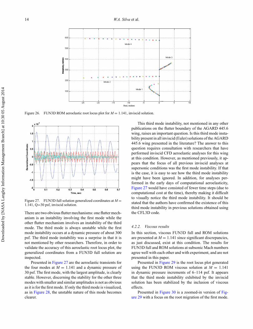
Figure 26. FUN3D ROM aeroelastic root locus plot for M = 1.141, inviscid solution.

Figure 27. FUN3D full solution generalized coordinates at M =1.141, Q=30 psf, inviscid solution.

There are two obvious flutter mechanisms: one flutter mech-anism is an instability involving the first mode while theother flutter mechanism involves an instability of the thirdmode. The third mode is always unstable while the firstmode instability occurs at a dynamic pressure of about 300psf. The third mode instability was a surprise in that it isnot mentioned by other researchers. Therefore, in order tovalidate the accuracy of this aeroelastic root locus plot, thegeneralized coordinates from a FUN3D full solution areinspected.

Presented in Figure 27 are the aeroelastic transients forthe four modes at M = 1.141 and a dynamic pressure of30 psf. The first mode, with the largest amplitude, is clearlystable. However, discerning the stability for the other threemodes with smaller and similar amplitudes is not as obviousas it is for the first mode. If only the third mode is visualized,as in Figure 28, the unstable nature of this mode becomesclearer.

This third mode instability, not mentioned in any otherpublications on the flutter boundary of the AGARD 445.6wing, raises an important question. Is this third mode insta-bility present in all inviscid (Euler) solutions of the AGARD445.6 wing presented in the literature? The answer to thisquestion requires consultation with researchers that haveperformed inviscid CFD aeroelastic analyses for this wingat this condition. However, as mentioned previously, it ap-pears that the focus of all previous inviscid analyses atsupersonic conditions was the first mode instability. If thatis the case, it is easy to see how the third mode instabilitymight have been ignored. In addition, for analyses per-formed in the early days of computational aeroelasticity,Figure 27 would have consisted of fewer time steps (due tocomputational cost at the time), thereby making it difficultto visually notice the third mode instability. It should bestated that the authors have confirmed the existence of thisthird mode instability in previous solutions obtained usingthe CFL3D code.

4.2.2. Viscous results

In this section, viscous FUN3D full and ROM solutionsare presented at M = 1.141 since significant discrepancies,as just discussed, exist at this condition. The results forFUN3D full and ROM solutions at subsonic Mach numbersagree well with each other and with experiment, and are notpresented in this paper.

Presented in Figure 29 is the root locus plot generatedusing the FUN3D ROM viscous solution at M = 1.141in dynamic pressure increments of 6–114 psf. It appearsthat the third mode instability exhibited by the inviscidsolution has been stabilized by the inclusion of viscouseffects.

Presented in Figure 30 is a zoomed-in version of Fig-ure 29 with a focus on the root migration of the first mode.

Dow

nloa

ded

by [

NA

SA L

angl

ey I

nfor

mat

ion

Man

agem

ent B

ranc

h] a

t 10:

30 0

5 A

ugus

t 201

4

International Journal of Computational Fluid Dynamics 15

Figure 28. FUN3D full solution third generalized coordinate at M = 1.141, Q = 30 psf, inviscid solution.

As can be seen, the first mode is stable throughout thesedynamic pressures. However, a zoomed-in version of Fig-ure 29 with a focus on the root migration of the third mode,presented in Figure 31, indicates that initially, the thirdmode exhibits a slight instability before becoming morestable.

The four generalized coordinates from a FUN3D fullviscous solution, at Q = 6 psf, are presented as Figure 32. Atthis low dynamic pressure, all four generalized coordinatesare lowly damped. Figures 33 and 34 present the first andthird generalized coordinates from Figure 32, respectively.Visual analysis of both of these generalized coordinates

Figure 29. Viscous FUN3D ROM root locus plot at M = 1.141.

Dow

nloa

ded

by [

NA

SA L

angl

ey I

nfor

mat

ion

Man

agem

ent B

ranc

h] a

t 10:

30 0

5 A

ugus

t 201

4

16 W.A. Silva et al.

Figure 30. Viscous FUN3D ROM root locus plot at M = 1.141,zoomed-in to the first mode.

indicates that these generalized coordinates appear to bestable, although lowly damped. However, it is importantto state a fundamental and important difference between aroot locus plot and the visual, or otherwise post-processed,analysis of generalized coordinates over a short period oftime. A root locus plot, by definition, exhibits the rootsof a system as time approaches infinity or as the systemreaches steady state. In contrast, the analysis of the initialtransient response of a generalized coordinate over a shortperiod of time can be deceiving as the response can changeif the response was viewed (or analysed) over a longerperiod of time. Therefore, based on the root locus plot atthis condition, it appears that the third mode is unstablealthough that is not apparent in Figure 34.

Figure 31. Viscous FUN3D ROM root locus plot at M = 1.141,zoomed-in to the third mode.

Figure 32. Generalized coordinates from viscous FUN3D fullsolution at M = 1.141 and Q = 6 psf.

Figure 33. First generalized coordinate from viscous FUN3Dfull solution at M = 1.141 and Q = 6 psf.

Figure 34. Third generalized coordinate from viscous FUN3Dfull solution at M = 1.141 and Q = 6 psf.

Dow

nloa

ded

by [

NA

SA L

angl

ey I

nfor

mat

ion

Man

agem

ent B

ranc

h] a

t 10:

30 0

5 A

ugus

t 201

4

International Journal of Computational Fluid Dynamics 17

5. Concluding remarks

A comparison of linear, inviscid, and viscous aeroelasticsolutions for the AGARD 445.6 wing was presented. Thelinear solutions were generated using the linear equationsavailable within the CAP-TSD code. The inviscid and vis-cous solutions were generated using the FUN3D code. Theresults presented consisted of two types of solutions: fullCFD solutions whereby the CFD aeroelastic solution wascomputed in the standard time iterative approach and ROMsolutions whereby unsteady aerodynamic and aeroelasticROMs were generated using FUN3D and used to generateaeroelastic root locus plots as a function of dynamic pres-sure. An important conclusion from this research is thatvisualization of the aeroelastic root locus plots providedby the ROM approach enables a direct and more compre-hensive interpretation of the aeroelastic behaviour. Case inpoint, for the inviscid (Euler) solutions, the third mode isalways unstable while the flutter instability associated withthe first mode does not occur until about 300 psf. If thisthird mode instability is present in all inviscid solutionspublished by other researchers is not known at this pointin time. However, the importance of being able to view aroot locus plot in addition to time domain responses of thegeneralized coordinates was well established with this par-ticular result. Another related conclusion to be made is thatthe standard approach of viewing (and analysing) a shorttime history of the initial transient response of generalizedcoordinates may not be sufficiently accurate since it is pos-sible that the steady-state response has not been reachedover this short time interval. Here again, the use of the rootlocus plots generated using the ROM approach enable thecomplete observation of the aeroelastic response since, bydefinition, the root locus plots represent the dynamics ofthe system at the final steady state of the system.

ReferencesAdams, W. M., and S. T. Hoadley. 1993. “ISAC: A

Tool for Aeroservoelastic Modeling and Analysis,” Pa-per presented at the 34th Structures, Structural Dynam-ics, and Materials Conference, La Jolla, CA. AIAA PaperNo. 1993-1421.

Anderson, W. K., and D. L. Bonhaus. 1994. “An Implicit UpwindAlgorithm for Computing Turbulent Flows on UnstructuredGrids.” Computers and Fluids 23(1): 1–21.

Balajewicz, M., F. Nitzche, and D. Feszty. 2009. “Reduced Or-der Modeling of Nonlinear Transonic Aerodynamics Us-ing a Pruned Volterra Series.” Paper presented at the 50thAIAA/ASME/ASCE/AHS/ASC Structures, Structural Dy-namics, and Materials Conference, Palm Springs, CA. AIAAPaper No. 2009-2319.

Batina, J. T., D. A. Seidel, S. R. Bland, and R. Bennet. 1987.“Unsteady Transonic Flow Calculations for Realistic AircraftConfigurations.” Paper presented at the 28th Structures, Struc-tural Dynamics and Materials Conference, Monterey, CA,USA. AIAA Paper 1987-0850.

Bennett, R. M., J. T. Batina, and H. J. Cunningham. 1989. “Wing-Flutter Calculations with the CAP-TSD Unsteady Transonic

Small-Disturbance Program.” Journal of Aircraft 26(9): 876–882.

Bennett, R. M., and R. N. Desmarais. 1975. “Curve Fitting ofAeroelastic Transient Response Data with Exponential Func-tions.” In Flutter Testing Techniques, 43–58. NASA SP–415.Washington, D.C.: NASA.

Beran, P. S., and W. A. Silva. 2001. “Reduced-Order Model-ing: New Approaches for Computational Physics.” Paper pre-sented at the 39th AIAA Aerospace Sciences Meeting, Reno,NV, January 8–11.

Biedron, R. T., and J. Thomas. 2009. “Recent Enhancements to theFUN3D Flow Solver for Moving-Mesh Applications.” Paperpresented at the 47th AIAA Aerospace Sciences Meeting,Orlando, FL, January 5–8. AIAA Paper No. 2009-1360.

Chwalowski, P., J. P. Florance, J. Heeg, C. D. Wieseman, andB. Perry. 2011. “Preliminary Computational Analysis of theHIRENASD Configuration in Preparation for the AeroelasticPrediction Workshop.” Paper presented at the InternationalForum on Aeroelasticity and Structural Dynamics, Paris, June26. IFASD- 2011-108.

Cunningham, H. J., J. T. Batina, and R. M. Bennett. 1988. “Mod-ern Wing Flutter Analysis by Computational Fluid DynamicsMethod.” Journal of Aircraft 25(10): 962–968.

Edwards, J. R. 1995. “A Low-Diffusion Flux-Splitting Schemefor Navier-Stokes Calculations.” Paper presented at the 12thComputational Fluid Dynamics Conference, San Diego, CA,USA. AIAA Paper No. 1995–1703.

Ghoreyshi, M., M. L. Post, R. M. Cummings, A. D. Ronch, and K.J. Badcock. 2012. “Transonic Aerodynamic Loads Modelingof X-31 Aircraft.” Paper presented at the 30th Applied Aero-dynamics Conference, New Orleans, LA, June. AIAA PaperNo. 2012-3127.

Gupta, K. K. 1996. “Development of a Finite Element AeroelasticAnalysis Capability.” Journal of Aircraft 33(5): 995–1002.

Jirasek, A., and R. M. Cummings. 2009. “Application of VolterraFunctions to X-31 Aircraft Model Motion.” Paper presentedat the 27th Applied Aerodynamics Conference, San Antonio,TX, June. AIAA Paper No. 2009-3629.

Juang, J.-N,. 1994. Applied System Identification. EnglewoodCliffs, New Jersey: Prentice-Hall PTR.

Juang, J.-N., and Pappa, R. S. 1985. “An Eigensystem Realiza-tion Algorithm for Modal Parameter Identification and ModelReduction,” Journal of Guidance, Control, and Dynamics 8:620–627.

Juang, J.-N., M. Phan, L. G. Horta, and R. W. Longman. 1993.“Identification of Observer/Kalman Filter Markov Parame-ters: Theory and Experiments.” Journal of Guidance, Control,and Dynamics 16: 320–329.

Kim, T., M. Hong, K. G. Bhatia, and G. Sen Gupta. 2005. “Aeroe-lastic Model Reduction for Affordable Computational FluidDynamics-Based Flutter Analysis.” AIAA Journal 43: 2487–2495.

Krist, S. L., R. T. Biedron, and C. L. Rumsey. 1997. “CFL3DUser’s Manual Version 5.0.” Hampton, VA: Tech. rep. NASALangley Research Center.

Lee-Rausch, E. M., and J. T. Batina. 1993. “Calculation ofAGARD Wing 445.6 Flutter Using Navier-Stokes Aerody-namics.” Paper presented at the 11th Applied AerodynamicsConference, Monterey, CA, USA, January. AIAA Paper No.1993-3476.

Lee-Rausch, E. M., and J. T. Batina. 1995. “Wing Flutter Bound-ary Prediction Using Unsteady Euler Aerodynamic Method.”Journal of Aircraft 32(3): 416–422.

Milanese, A., and P. Marzocca. 2009. “Volterra Kernels Identi-fication Using Continuous Time Impulses Applied to Non-linear Aeroelastic Problems.” Paper presented at the 50th

Dow

nloa

ded

by [

NA

SA L

angl

ey I

nfor

mat

ion

Man

agem

ent B

ranc

h] a

t 10:

30 0

5 A

ugus

t 201

4

18 W.A. Silva et al.

AIAA/ASME/ASCE/AHS/ASC Structures, Structural Dy-namics, and Materials Conference, Palm Springs, CA, May4–7.

Omran, A., and B. Newman. 2009. “Piecewise Global VolterraNonlinear Modeling and Characterization for Aircraft Dy-namics.” Journal of Guidance, Control, and Dynamics 32(3):749–759.

Pahlavanloo, P. 2007. “Dynamic Aeroelastic Simulation of theAGARD 445.6 Wing Using Edge.” Technical Report FOI-R-2259-SE, April. Stockholm, Sweden: FOI, Defence ResearchAgency.

Pirzadeh, S. Z. 2008. “Advanced Unstructured Grid Generation forComplex Aerodynamic Applications.” Paper presented at the26th AIAA Applied Aerodynamics Conference, Honolulu,HI, USA, August. AIAA Paper No. 2008-7178.

Raveh, D. E. 2004. “Identification of Computational-Fluid-Dynamic Based Unsteady Aerodynamic Models for Aeroe-lastic Analysis.” Journal of Aircraft 41: 620–632.

Raveh, D. E., Y. Levy, and M. Karpel. 2000. “Aircraft AeroelasticAnalysis and Design Using CFD-Based Unsteady Loads.” Pa-per presented at the 41st Structures, Structural Dynamics, andMaterials Conference, Atlanta, GA, April. Paper No. 2000-1325.

“Registered Product of the MathWorks, Inc.”Samareh, J. A. 1993. “Unstructured Grids on NURBS Surfaces.”

Paper presented at the 11th Applied Aerodynamics Confer-ence, Monterey, CA, USA. AIAA Paper 1993-3454.

Samareh, J. A. 2007. “Discrete Data Transfer Technique forFluid-Structure Interaction.” Paper presented at the 18thAIAA Computational Fluid Dynamics Conference, Miami,FL, USA. AIAA Paper 2007-4309, June.

Silva, W. A. 1993. “Application of Nonlinear Systems Theoryto Transonic Unsteady Aerodynamic Responses.” Journal ofAircraft 30: 660–668.

Silva, W. A. 1997. “Discrete-Time Linear and Nonlinear Aerody-namic Impulse Responses for Efficient CFD Analyses.” PhDthesis, College of William & Mary.

Silva, W. A. 1999. “Reduced-Order Models Based on Lin-ear and Nonlinear Aerodynamic Impulse Responses.”CEAS/AIAA/ICASE/NASA International Forum on Aeroe-lasticity and Structural Dynamics, Williamsburg, VA, USA,June.

Silva, W. A. 2005. “Identification of Nonlinear Aeroelastic Sys-tems Based on the Volterra Theory: Progress and Opportuni-ties.” Journal of Nonlinear Dynamics 39: 25–62.

Silva, W. A. 2007. “Recent Enhancements to the Development ofCFD-Based Aeroelastic Reduced Order Models.” Paper pre-

sented at the 48th AIAA/ASME/ASCE/AHS/ASC Structures,Structural Dynamics, and Materials Conference, Honolulu,HI, April 23–26. AIAA Paper No. 2007-2051.

Silva, W. A. 2008. “Simultaneous Excitation of Multiple-Input/Multiple-Output CFD-Based Unsteady AerodynamicSystems.” Journal of Aircraft 45(4): 1267–1274.

Silva, W. A., and R. E. Bartels. 2004. “Development of Reduced-Order Models for Aeroelastic Analysis and Flutter PredictionUsing the CFL3Dv6.0 Code.” Journal of Fluids and Struc-tures, no. 19: 729–745.

Silva, W. A., and R. M. Bennett. 1995. “Application of Tran-sonic Small Disturbance Theory to the Active Flexible WingModel.” Journal of Aircraft 32(1): 16–22.

Silva, W. A., P. S. Beran, C. E. S. Cesnik, R. E. Guendel, A.Kurdila, R. J. Prazenica, L. Librescu, P. Marzocca, and D.Raveh. 2001. “Reduced-Order Modeling: Cooperative Re-search and Development at the NASA Langley ResearchCenter.” CEAS/AIAA/ICASE/NASA International Forumon Aeroelasticity and Structural Dynamics, Madrid, Spain,June.

Silva, W. A., V. N. Vatsa, and R. T. Biedron. 2009. “Develop-ment of Unsteady Aerodynamic and Aeroelastic Reduced-Order Models Using the FUN3D Code.” Paper presented atthe International Forum on Aeroelasticity and Structural Dy-namics, Seattle, WA, June 2009. IFASD Paper No. 2009–30.

Silva, W. A., V. N. Vatsa, and R. T. Biedron. 2010. “Reduced-OrderModels for the Aeroelastic Analyses of the Ares Vehicles.”Paper presented at the 28th AIAA Applied AerodynamicsConference, Chicago, IL, June 2010. AIAA Paper No. 2010-4375.

Spalart, P. R., and S. R. Allmaras. 1994. “A One-Equation Turbu-lence Model for Aerodynamic Flows.” La Recherche Aerospa-tiale, no. 1: 5–21.

Vatsa, V. N., and J. A. White. 2009. “Calibration of a UnifiedFlux Limiter for Ares-Class Launch Vehicles from Subsonicto Supersonic Speeds.” Presented at the Joint ARMY-NAVY-NASA-Air Force, Las Vegas, NV, USA, April. JANNAF PaperNo. 2009.

Yates, C. E. 1988. “AGARD Standard Aeroelastic Configurationsfor Dynamic Response – Wing 445.6.” AGARD Report No.765. Hampton, VA: NASA.

Yates, C. E., Land, N. S., and J. T. Foughner, J,. 1963. “Measuredand Calculated Subsonic and Transonic Flutter Characteristicsof a 45-degree Swept-Back Wing Planform in Air and inFreon-12 in the Langley Transonic Dynamics Tunnel.” Tech.Rep. No. TN D-1616. Hampton, VA: NASA.

Dow

nloa

ded

by [

NA

SA L

angl

ey I

nfor

mat

ion

Man

agem

ent B

ranc

h] a

t 10:

30 0

5 A

ugus

t 201

4