Probability and Stochastic Processes - WINLABryates/student3e/quizsol3i.pdf · Probability and...
90
Probability and Stochastic Processes A Friendly Introduction for Electrical and Computer Engineers Third Edition International Students’ Version QUIZ SOLUTIONS Roy D. Yates, David J. Goodman, David Famolari April 30, 2014 1
Transcript of Probability and Stochastic Processes - WINLABryates/student3e/quizsol3i.pdf · Probability and...
Probability and Stochastic Processes
A Friendly Introduction for Electrical and Computer Engineers
Third Edition
International Students’ Version
QUIZ SOLUTIONS
Roy D. Yates, David J. Goodman, David Famolari
April 30, 2014
1

Comments on the Quiz Solutions
• Matlab functions used in the text or in these quiz solutions can be found inthe archive matcode3e.zip. This archive is available for download from theJohn Wiley companion website. Two other documents of interest are alsoavailable for download:
– The Student Solutions Manual studentsolns3i.pdf.
– Amanual probmatlab3e.pdf describing the .m functions in matcode3e.zip.
• This manual uses a page size matched to the screen of an iPad tablet. If youdo print on paper and you have good eyesight, you may wish to print twopages per sheet in landscape mode. On the other hand, a “Fit to Paper”printing option will create “Large Print” output.
• Send error reports, suggestions, or comments to
2
Quiz 1.1 Solution
A1 = {vvv, vvd, dvv, dvd}B1 = {vdv, vdd, ddv, ddd}A2 = {vvv, ddd}B2 = {vdv, dvd}A3 = {vvv, vvd, vdv, dvv, vdd, dvd, ddv}B3 = {ddd, ddv, dvd, vdd}
Recall that Ai and Bi are collectively exhaustive if Ai∪Bi = S. Also, Ai andBi are mutually exclusive if Ai ∩ Bi = φ. Since we have written down eachpair Ai and Bi above, we can simply check for these properties.
The pair A1 and B1 are mutually exclusive and collectively exhaustive. Thepair A2 and B2 are mutually exclusive but not collectively exhaustive. Thepair A3 and B3 are not mutually exclusive since dvd belongs to A3 and B3.However, A3 and B3 are collectively exhaustive.
Quiz 1.2 Solution
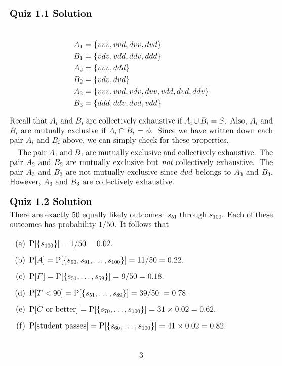
There are exactly 50 equally likely outcomes: s51 through s100. Each of theseoutcomes has probability 1/50. It follows that
(a) P[{s100}] = 1/50 = 0.02.
(b) P[A] = P[{s90, s91, . . . , s100}] = 11/50 = 0.22.
(c) P[F ] = P[{s51, . . . , s59}] = 9/50 = 0.18.
(d) P[T < 90] = P[{s51, . . . , s89}] = 39/50. = 0.78.
(e) P[C or better] = P[{s70, . . . , s100}] = 31× 0.02 = 0.62.
(f) P[student passes] = P[{s60, . . . , s100}] = 41× 0.02 = 0.82.
3
Quiz 1.3 Solution
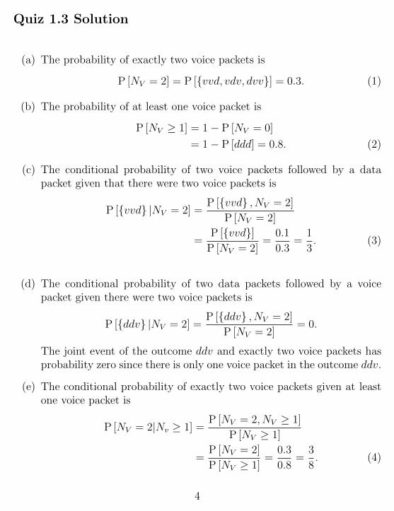
(a) The probability of exactly two voice packets is
P [NV = 2] = P [{vvd, vdv, dvv}] = 0.3. (1)
(b) The probability of at least one voice packet is
P [NV ≥ 1] = 1− P [NV = 0]
= 1− P [ddd] = 0.8. (2)
(c) The conditional probability of two voice packets followed by a datapacket given that there were two voice packets is
P [{vvd} |NV = 2] =P [{vvd} , NV = 2]
P [NV = 2]
=P [{vvd}]
P [NV = 2]=
0.1
0.3=
1
3. (3)
(d) The conditional probability of two data packets followed by a voicepacket given there were two voice packets is
P [{ddv} |NV = 2] =P [{ddv} , NV = 2]
P [NV = 2]= 0.
The joint event of the outcome ddv and exactly two voice packets hasprobability zero since there is only one voice packet in the outcome ddv.
(e) The conditional probability of exactly two voice packets given at leastone voice packet is
P [NV = 2|Nv ≥ 1] =P [NV = 2, NV ≥ 1]
P [NV ≥ 1]
=P [NV = 2]
P [NV ≥ 1]=
0.3
0.8=
3
8. (4)
4
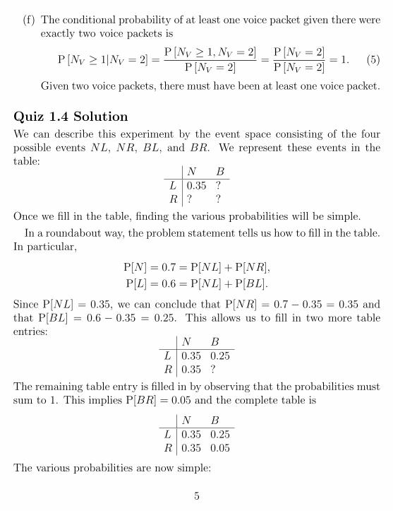
(f) The conditional probability of at least one voice packet given there wereexactly two voice packets is
P [NV ≥ 1|NV = 2] =P [NV ≥ 1, NV = 2]
P [NV = 2]=
P [NV = 2]
P [NV = 2]= 1. (5)
Given two voice packets, there must have been at least one voice packet.
Quiz 1.4 SolutionWe can describe this experiment by the event space consisting of the fourpossible events NL, NR, BL, and BR. We represent these events in thetable:
N BL 0.35 ?R ? ?
Once we fill in the table, finding the various probabilities will be simple.
In a roundabout way, the problem statement tells us how to fill in the table.In particular,
P[N ] = 0.7 = P[NL] + P[NR],
P[L] = 0.6 = P[NL] + P[BL].
Since P[NL] = 0.35, we can conclude that P[NR] = 0.7 − 0.35 = 0.35 andthat P[BL] = 0.6 − 0.35 = 0.25. This allows us to fill in two more tableentries:
N BL 0.35 0.25R 0.35 ?
The remaining table entry is filled in by observing that the probabilities mustsum to 1. This implies P[BR] = 0.05 and the complete table is
N BL 0.35 0.25R 0.35 0.05
The various probabilities are now simple:
5
(a) P [B ∪ L] = P [NL] + P [BL] + P [BR]
= 0.35 + 0.25 + 0.05 = 0.65.
(b) P [N ∪ L] = P [N ] + P [L]− P [NL]
= 0.7 + 0.6− 0.35 = 0.95.
(c) P [N ∪B] = P [S] = 1.
(d) P [LR] = P [LLc] = 0.
Quiz 1.5 Solution
In this experiment, there are four outcomes with probabilities
P[{vv}] = (0.8)2 = 0.64, P[{vd}] = (0.8)(0.2) = 0.16,
P[{dv}] = (0.2)(0.8) = 0.16, P[{dd}] = (0.2)2 = 0.04.
When checking the independence of any two events A and B, it’s wise toavoid intuition and simply check whether P[AB] = P[A] P[B]. Using theprobabilities of the outcomes, we now can test for the independence of events.
(a) First, we calculate the probability of the joint event:
P [NV = 2, NV ≥ 1] = P [NV = 2] = P [{vv}] = 0.64. (1)
Next, we observe that P[NV ≥ 1] = P[{vd, dv, vv}] = 0.96.. Finally, wemake the comparison
P [NV = 2] P [NV ≥ 1] = (0.64)(0.96) 6= P [NV = 2, NV ≥ 1] , (2)
which shows the two events are dependent.
(b) The probability of the joint event is
P [NV ≥ 1, C1 = v] = P [{vd, vv}] = 0.80. (3)
6
From part (a), P[NV ≥ 1] = 0.96. Further, P[C1 = v] = 0.8 so that
P [NV ≥ 1] P [C1 = v] = (0.96)(0.8) = 0.768 6= P [NV ≥ 1, C1 = v] .(4)
Hence, the events are dependent.
(c) The problem statement that the packets were independent implies thatthe events {C2 = v} and {C1 = d} are independent events. Just to besure, we can do the calculations to check:
P [C1 = d, C2 = v] = P [{dv}] = 0.16. (5)
Since P[C1 = d] P[C2 = v] = (0.2)(0.8) = 0.16, we confirm that theevents are independent. Note that this shouldn’t be surprising since weused the information that the packets were independent in the problemstatement to determine the probabilities of the outcomes.
(d) The probability of the joint event is
P [C2 = v,NV is even] = P [{vv}] = 0.64. (6)
Also, each event has probability
P [C2 = v] = P [{dv, vv}] = 0.8, (7)
P [NV is even] = P [{dd, vv}] = 0.68. (8)
Thus,
P [C2 = v] P [NV is even] = (0.8)(0.68)
= 0.544 6= P [C2 = v,NV is even] . (9)
Thus the events are dependent.
7
Quiz 1.6 Solution
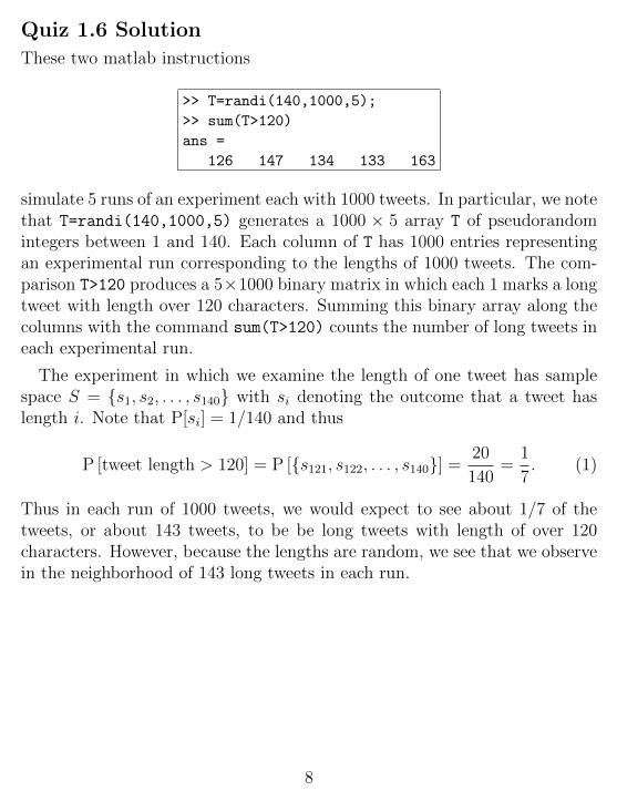
These two matlab instructions
>> T=randi(140,1000,5);
>> sum(T>120)
ans =
126 147 134 133 163
simulate 5 runs of an experiment each with 1000 tweets. In particular, we notethat T=randi(140,1000,5) generates a 1000 × 5 array T of pseudorandomintegers between 1 and 140. Each column of T has 1000 entries representingan experimental run corresponding to the lengths of 1000 tweets. The com-parison T>120 produces a 5×1000 binary matrix in which each 1 marks a longtweet with length over 120 characters. Summing this binary array along thecolumns with the command sum(T>120) counts the number of long tweets ineach experimental run.
The experiment in which we examine the length of one tweet has samplespace S = {s1, s2, . . . , s140} with si denoting the outcome that a tweet haslength i. Note that P[si] = 1/140 and thus
P [tweet length > 120] = P [{s121, s122, . . . , s140}] =20
140=
1
7. (1)
Thus in each run of 1000 tweets, we would expect to see about 1/7 of thetweets, or about 143 tweets, to be be long tweets with length of over 120characters. However, because the lengths are random, we see that we observein the neighborhood of 143 long tweets in each run.
8
Quiz 2.1 Solution
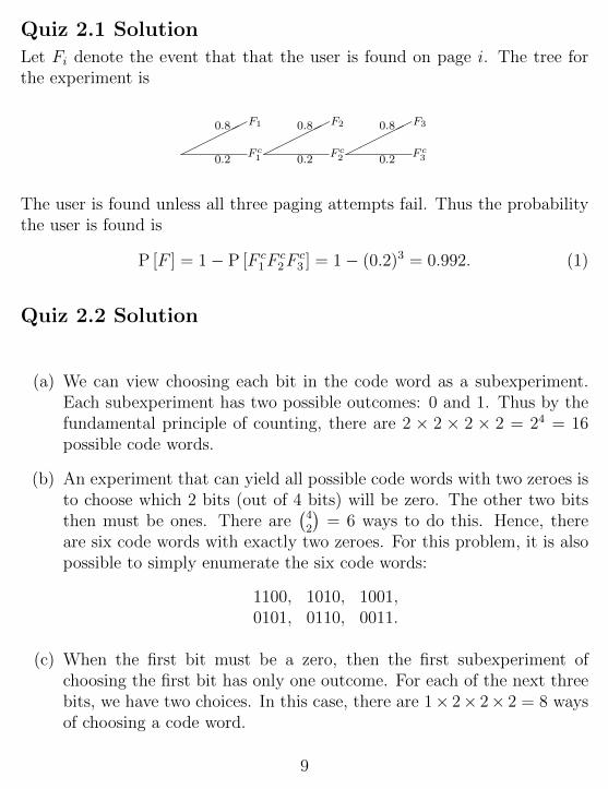
Let Fi denote the event that that the user is found on page i. The tree forthe experiment is
�����F10.8
F c10.2��
���F20.8
F c20.2��
���F30.8
F c30.2
The user is found unless all three paging attempts fail. Thus the probabilitythe user is found is
P [F ] = 1− P [F c1F
c2F
c3 ] = 1− (0.2)3 = 0.992. (1)
Quiz 2.2 Solution
(a) We can view choosing each bit in the code word as a subexperiment.Each subexperiment has two possible outcomes: 0 and 1. Thus by thefundamental principle of counting, there are 2 × 2 × 2 × 2 = 24 = 16possible code words.
(b) An experiment that can yield all possible code words with two zeroes isto choose which 2 bits (out of 4 bits) will be zero. The other two bitsthen must be ones. There are
(42
)= 6 ways to do this. Hence, there
are six code words with exactly two zeroes. For this problem, it is alsopossible to simply enumerate the six code words:
1100, 1010, 1001,0101, 0110, 0011.
(c) When the first bit must be a zero, then the first subexperiment ofchoosing the first bit has only one outcome. For each of the next threebits, we have two choices. In this case, there are 1× 2× 2× 2 = 8 waysof choosing a code word.
9
(d) For the constant ratio code, we can specify a code word by choosingM of the bits to be ones. The other N −M bits will be zeroes. Thenumber of ways of choosing such a code word is
(NM
). For N = 8 and
M = 3, there are(83
)= 56 code words.
Quiz 2.3 Solution
(a) In this problem, k bits received in error is the same as k failures in 100trials. The failure probability is ε = 1 − p and the success probabilityis 1 − ε = p. That is, the probability of k bits in error and 100 − kcorrectly received bits is
P [Ek,100−k] =
(100
k
)εk(1− ε)100−k. (1)
For ε = 0.01,
P [E0,100] = (1− ε)100 = (0.99)100 = 0.3660. (2)
P [E1,99] = 100(0.01)(0.99)99 = 0.3700. (3)
P [E2,98] = 4950(0.01)2(0.99)98 = 0.1849. (4)
P [E3,97] = 161, 700(0.01)3(0.99)97 = 0.0610. (5)
(b) The probability a packet is decoded correctly is just
P [C] = P [E0,100] + P [E1,99] + P [E2,98] + P [E3,97] = 0.9819. (6)
Quiz 2.4 Solution
For a Matlab simulation, we first generate a vector R of 100 random num-bers. Second, we generate vector X as a function of R to represent the 3possible outcomes of a flip. That is, X(i)=1 if flip i was heads, X(i)=2 if flipi was tails, and X(i)=3) is flip i landed on the edge. The matlab code is
10
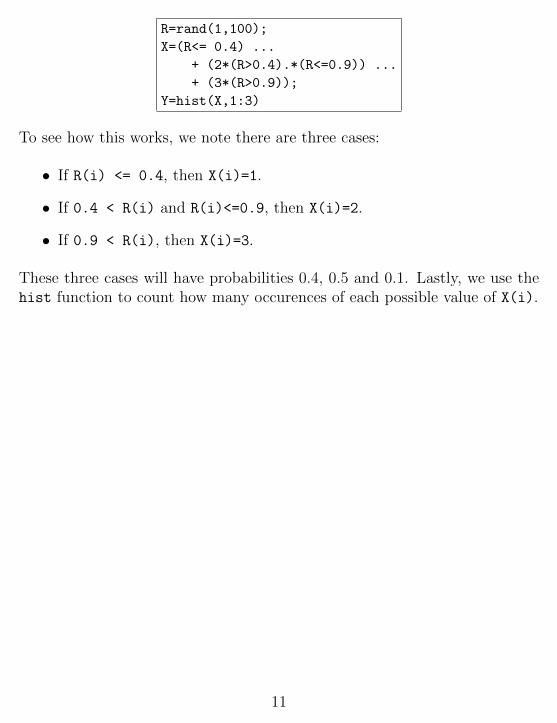
R=rand(1,100);
X=(R<= 0.4) ...
+ (2*(R>0.4).*(R<=0.9)) ...
+ (3*(R>0.9));
Y=hist(X,1:3)
To see how this works, we note there are three cases:
• If R(i) <= 0.4, then X(i)=1.
• If 0.4 < R(i) and R(i)<=0.9, then X(i)=2.
• If 0.9 < R(i), then X(i)=3.
These three cases will have probabilities 0.4, 0.5 and 0.1. Lastly, we use thehist function to count how many occurences of each possible value of X(i).
11
Quiz 3.1 SolutionThe sample space, probabilities and corresponding grades for the experimentare
Outcomes BB BC CB CCG2 3.0 2.5 2.5 2.0
Quiz 3.2 Solution
(a) To find c, we recall that the PMF must sum to 1. That is,
3∑n=1
PN (n) = c
(1 +
1
2+
1
3
)= 1. (1)
This implies c = 6/11. Now that we have found c, the remaining partsare straightforward.
(b) P[N = 1] = PN(1) = c = 6/11.
(c) P [N ≥ 2] = PN (2) + PN (3)
= c/2 + c/3 = 5/11.
(d) P[N > 3] =∑∞
n=4 PN(n) = 0.
Quiz 3.3 SolutionDecoding each transmitted bit is an independent trial where we call a biterror a “success.” Each bit is in error, that is, the trial is a success, withprobability p. Now we can interpret each experiment in the generic contextof independent trials.
(a) The random variable X is the number of trials up to and including thefirst success. Similar to Example 3.8, X has the geometric PMF
PX(x) =
{p(1− p)x−1 x = 1, 2, . . .
0 otherwise.
12
(b) If p = 0.1, then the probability exactly 10 bits are sent is
PX (10) = (0.1)(0.9)9 = 0.0387. (1)
The probability that at least 10 bits are sent is
P [X ≥ 10] =∞∑
x=10
PX (x) . (2)
This sum is not too hard to calculate. However, its even easier toobserve that X ≥ 10 if the first 10 bits are transmitted correctly. Thatis,
P [X ≥ 10] = P [first 10 bits correct] = (1− p)10. (3)
For p = 0.1,
P [X ≥ 10] = 0.910 = 0.3487. (4)
(c) The random variable Y is the number of successes in 100 independenttrials. Just as in Example 3.9, Y has the binomial PMF
PY (y) =
(100
y
)py(1− p)100−y. (5)
If p = 0.01, the probability of exactly 2 errors is
PY (2) =
(100
2
)(0.01)2(0.99)98 = 0.1849. (6)
(d) The probability of no more than 2 errors is
P [Y ≤ 2] = PY (0) + PY (1) + PY (2)
= (0.99)100 + 100(0.01)(0.99)99 +
(100
2
)(0.01)2(0.99)98
= 0.9207. (7)
13
(e) Random variable Z is the number of trials up to and including the thirdsuccess. Thus Z has the Pascal PMF (see Example 3.10)
PZ (z) =
(z − 1
2
)p3(1− p)z−3. (8)
Note that PZ(z) > 0 for z = 3, 4, 5, . . ..
(f) If p = 0.25, the probability that the third error occurs on bit 12 is
PZ (12) =
(11
2
)(0.25)3(0.75)9 = 0.0645. (9)
Quiz 3.4 Solution
Each of these probabilities can be read from the graph of the CDF FY(y).However, we must keep in mind that when FY(y) has a discontinuity at y0,FY(y) takes the upper value FY(y+0 ).
(a) P[Y < 1] = FY(1−) = 0.
(b) P[Y ≤ 1] = FY(1) = 0.6.
(c) P[Y > 2] = 1− P[Y ≤ 2] = 1− FY(2) = 1− 0.8 = 0.2.
(d) P[Y ≥ 2] = 1− P[Y < 2] = 1− FY(2−) = 1− 0.6 = 0.4.
(e) P[Y = 1] = P[Y ≤ 1]− P[Y < 1] = FY(1+)− FY(1−) = 0.6.
(f) P[Y = 3] = P[Y ≤ 3]− P[Y < 3] = FY(3+)− FY(3−) = 0.8− 0.8 = 0.
Quiz 3.5 Solution
14
(a) With probability 1/3, the subscriber sends a text and the cost is C = 10cents. Otherwise, with probability 2/3, the subscriber receives a textand the cost is C = 5 cents. This corresponds to the PMF
PC (c) =
2/3 c = 5,
1/3 c = 10,
0 otherwise.
(1)
(b) The expected value of C is
E [C] = (2/3)(5) + (1/3)(10) = 6.67 cents. (2)
(c) For the next two parts we think of each text as a Bernoulli trial suchthat the trial is a “success” if the subscriber sends a text. The successprobability is p = 1/3. Let R denote the number of texts received beforesending a text. In terms of Bernoulli trials, R is the number of failuresbefore the first success. R is similar to a geometric random variableexcept R = 0 is possible if the first text is sent rather than received. Ingeneral R = r if the first r trials are failures (i.e. the first r texts arereceived) and trial r + 1 is a success. Thus R has PMF
PR(r) =
{(1− p)rp r = 0, 1, 2 . . .
0 otherwise.(3)
The probability of receiving four texts before sending a text is
PR(4) = (1− p)4p. (4)
(d) The expected number of texts received before sending a text is
E [R] =∞∑r=0
rPR(r) =∞∑r=0
r(1− p)rp. (5)
15
Letting q = 1− p and observing that the r = 0 term in the sum is zero,
E [R] = p∞∑r=1
rqr. (6)
Using Math Fact B.7, we have
E [R] = pq
(1− q)2=
1− pp
= 2. (7)
Quiz 3.6 Solution
(a) As a function of N , the money spent by the tree customers is
M = 450N + 300(3−N) = 900 + 150N.
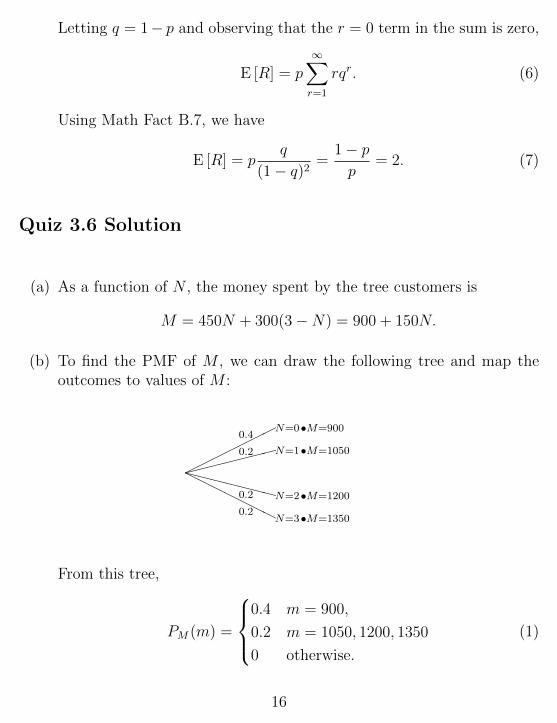
(b) To find the PMF of M , we can draw the following tree and map theoutcomes to values of M :
�����
��N=0
0.4
HHHHHHHN=3
0.2
������
�N=10.2
XXXXXXXN=20.2
•M=900
•M=1050
•M=1200
•M=1350
From this tree,
PM (m) =
0.4 m = 900,
0.2 m = 1050, 1200, 1350
0 otherwise.
(1)
16
From the PMF PM(m), the expected value of M is
E [M ] = 900PM (900) + 1050PM (1050)
+ 1200PM (1200) + 1350PM (1350)
= (900)(0.4) + (1050 + 1200 + 1350)(0.2) = 1080. (2)
Quiz 3.7 Solution
(a) Using Definition 3.11, the expected number of applications is
E [A] =4∑
a=1
aPA(a)
= 1(0.4) + 2(0.3) + 3(0.2) + 4(0.1) = 2. (1)
(b) The number of memory chips is
M = g(A) =
4 A = 1, 2,
6 A = 3,
8 A = 4.
(2)
(c) By Theorem 3.10, the expected number of memory chips is
E [M ] =4∑
a=1
g(A)PA(a)
= 4(0.4) + 4(0.3) + 6(0.2) + 8(0.1) = 4.8. (3)
Since E[A] = 2,g(E[A]) = g(2) = 4.
However, E[M ] = 4.8 6= g(E[A]). The two quantities are differentbecause g(A) is not of the form αA+ β.
17
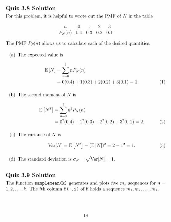
Quiz 3.8 Solution
For this problem, it is helpful to wrote out the PMF of N in the table
n 0 1 2 3PN (n) 0.4 0.3 0.2 0.1
The PMF PN(n) allows us to calculate each of the desired quantities.
(a) The expected value is
E [N ] =3∑
n=0
nPN (n)
= 0(0.4) + 1(0.3) + 2(0.2) + 3(0.1) = 1. (1)
(b) The second moment of N is
E[N2]
=3∑
n=0
n2PN (n)
= 02(0.4) + 12(0.3) + 22(0.2) + 32(0.1) = 2. (2)
(c) The variance of N is
Var[N ] = E[N2]− (E [N ])2 = 2− 12 = 1. (3)
(d) The standard deviation is σN =√
Var[N ] = 1.
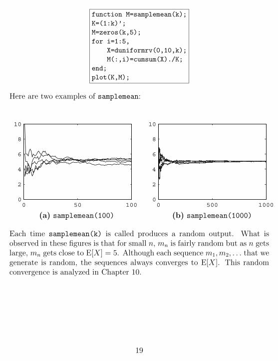
Quiz 3.9 Solution
The function samplemean(k) generates and plots five mn sequences for n =1, 2, . . . , k. The ith column M(:,i) of M holds a sequence m1,m2, . . . ,mk.
18
function M=samplemean(k);
K=(1:k)’;
M=zeros(k,5);
for i=1:5,
X=duniformrv(0,10,k);
M(:,i)=cumsum(X)./K;
end;
plot(K,M);
Here are two examples of samplemean:
0 50 1000
2
4
6
8
10
0 500 10000
2
4
6
8
10
(a) samplemean(100) (b) samplemean(1000)
Each time samplemean(k) is called produces a random output. What isobserved in these figures is that for small n, mn is fairly random but as n getslarge, mn gets close to E[X] = 5. Although each sequence m1,m2, . . . that wegenerate is random, the sequences always converges to E[X]. This randomconvergence is analyzed in Chapter 10.
19
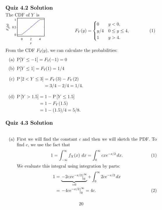
Quiz 4.2 SolutionThe CDF of Y is
0 2 4
0
0.5
1
y
FY(y
)
FY (y) =
0 y < 0,
y/4 0 ≤ y ≤ 4,
1 y > 4.
(1)
From the CDF FY(y), we can calculate the probabilities:
(a) P[Y ≤ −1] = FY(−1) = 0
(b) P[Y ≤ 1] = FY(1) = 1/4
(c) P [2 < Y ≤ 3] = FY (3)− FY (2)
= 3/4− 2/4 = 1/4.
(d) P [Y > 1.5] = 1− P [Y ≤ 1.5]
= 1− FY (1.5)
= 1− (1.5)/4 = 5/8.
Quiz 4.3 Solution
(a) First we will find the constant c and then we will sketch the PDF. Tofind c, we use the fact that
1 =
∫ ∞−∞
fX (x) dx =
∫ ∞0
cxe−x/2 dx. (1)
We evaluate this integral using integration by parts:
1 = −2cxe−x/2∣∣∞0︸ ︷︷ ︸
=0
+
∫ ∞0
2ce−x/2 dx
= −4ce−x/2∣∣∞0
= 4c. (2)
20
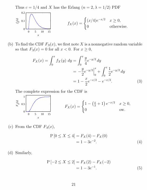
Thus c = 1/4 and X has the Erlang (n = 2, λ = 1/2) PDF
0 5 10 150
0.1
0.2
x
f X(x
)
fX (x) =
{(x/4)e−x/2 x ≥ 0,
0 otherwise.
(b) To find the CDF FX(x), we first noteX is a nonnegative random variableso that FX(x) = 0 for all x < 0. For x ≥ 0,
FX (x) =
∫ x
0
fX (y) dy =
∫ x
0
y
4e−y/2 dy
= −y2e−y/2
∣∣∣x0
+
∫ x
0
1
2e−y/2 dy
= 1− x
2e−x/2 − e−x/2. (3)
The complete expression for the CDF is
0 5 10 150
0.5
1
x
FX(x
)
FX (x) =
{1−
(x2
+ 1)e−x/2 x ≥ 0,
0 ow.
(c) From the CDF FX(x),
P [0 ≤ X ≤ 4] = FX (4)− FX (0)
= 1− 3e−2. (4)
(d) Similarly,
P [−2 ≤ X ≤ 2] = FX (2)− FX (−2)
= 1− 3e−1. (5)
21
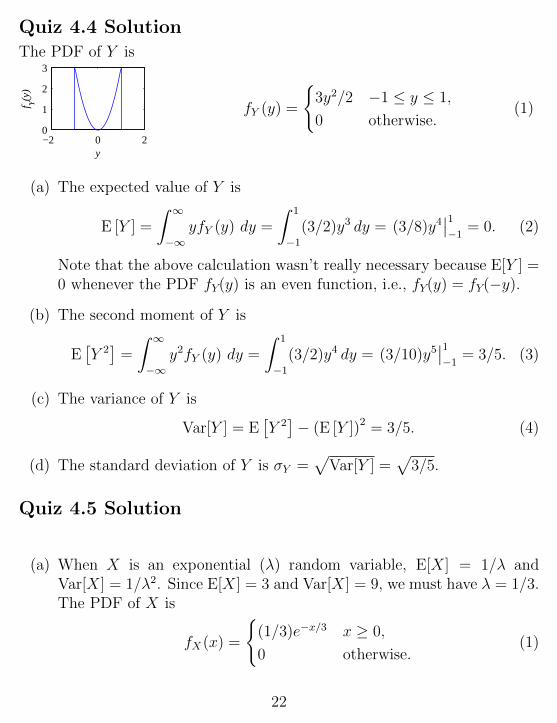
Quiz 4.4 SolutionThe PDF of Y is
−2 0 20
1
2
3
y
f Y(y
)
fY (y) =
{3y2/2 −1 ≤ y ≤ 1,
0 otherwise.(1)
(a) The expected value of Y is
E [Y ] =
∫ ∞−∞
yfY (y) dy =
∫ 1
−1(3/2)y3 dy = (3/8)y4
∣∣1−1 = 0. (2)
Note that the above calculation wasn’t really necessary because E[Y ] =0 whenever the PDF fY(y) is an even function, i.e., fY(y) = fY(−y).
(b) The second moment of Y is
E[Y 2]
=
∫ ∞−∞
y2fY (y) dy =
∫ 1
−1(3/2)y4 dy = (3/10)y5
∣∣1−1 = 3/5. (3)
(c) The variance of Y is
Var[Y ] = E[Y 2]− (E [Y ])2 = 3/5. (4)
(d) The standard deviation of Y is σY =√
Var[Y ] =√
3/5.
Quiz 4.5 Solution
(a) When X is an exponential (λ) random variable, E[X] = 1/λ andVar[X] = 1/λ2. Since E[X] = 3 and Var[X] = 9, we must have λ = 1/3.The PDF of X is
fX (x) =
{(1/3)e−x/3 x ≥ 0,
0 otherwise.(1)
22
(b) We know X is a uniform (a, b) random variable. To find a and b, weapply Theorem 4.6 to write
E [X] =a+ b
2= 3 (2)
Var[X] =(b− a)2
12= 9. (3)
This implies
a+ b = 6, b− a = ±6√
3. (4)
The only valid solution with a < b is
a = 3− 3√
3, b = 3 + 3√
3. (5)
The complete expression for the PDF of X is
fX (x) =
{1/(6√
3) 3− 3√
3 < x < 3 + 3√
3,
0 otherwise.(6)
(c) We know that the Erlang (n, λ) random variable has PDF
fX (x) =
{λnxn−1e−λx
(n−1)! x ≥ 0,
0 otherwise.(7)
The expected value and variance are E[X] = n/λ and Var[X] = n/λ2.This implies
n
λ= 3,
n
λ2= 9. (8)
It follows that
n = 3λ = 9λ2. (9)
Thus λ = 1/3 and n = 1. As a result, the Erlang (n, λ) random variablemust be the exponential (λ = 1/3) random variable with PDF
fX (x) =
{(1/3)e−x/3 x ≥ 0,
0 otherwise.(10)
23
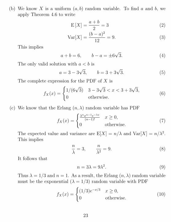
Quiz 4.6 SolutionThe PDFs of X and Y are:
−5 0 50
0.2
0.4
x yf X
(x)
fY(y
)
← fX(x)
← fY(y)
The fact that Y has twice the standard deviation of X is reflected in thegreater spread of fY(y). However, it is important to remember that as thestandard deviation increases, the peak value of the Gaussian PDF goes down.
Each of the requested probabilities can be calculated using Φ(z) functionand Table 4.1 or Q(z) and Table 4.2.
(a) Since X is Gaussian (0, 1),
P [−1 < X ≤ 1] = FX (1)− FX (−1)
= Φ(1)− Φ(−1)
= 2Φ(1)− 1 = 0.6826. (1)
(b) Since Y is Gaussian (0, 2),
P [−1 < Y ≤ 1] = FY (1)− FY (−1)
= Φ
(1
σY
)− Φ
(−1
σY
)= 2Φ
(1
2
)− 1 = 0.383. (2)
(c) Again, since X is Gaussian (0, 1), P[X > 3.5] = Q(3.5) = 2.33× 10⁻⁴.
(d) Since Y is Gaussian (0, 2),
P [Y > 3.5] = Q
(3.5
2
)= 1− Φ(1.75) = 0.04. (3)
24
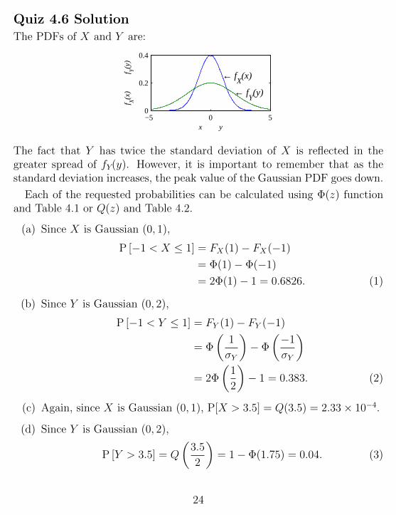
Quiz 4.7 Solution
The CDF of X is
−2 0 2
0
0.5
1
x
FX(x
)
FX (x) =
0 x < −1,
(x+ 1)/4 −1 ≤ x < 1,
1 x ≥ 1.
(1)
The following probabilities can be read directly from the CDF:
(a) P[X ≤ 1] = FX(1) = 1.
(b) P[X < 1] = FX(1−) = 1/2.
(c) P[X = 1] = FX(1+)− FX(1−) = 1/2.
(d) We find the PDF fY(y) by taking the derivative of FY(y). The resultingPDF is
−2 0 20
0.5
x
f X(x
)
0.5
fX (x) =
14
−1 ≤ x < 1,δ(x−1)
2x = 1,
0 otherwise.
(2)
Quiz 4.8 Solution
From Theorem 4.7, we know that if X is a continuous uniform (a − 1, b)random variable, then Y = dXe is a discrete uniform (a, b) random variable.A Matlab function that implements this solution to produce m samples ofa discrete uniform (a, b) random variable is:
function y = duniformrv(a,b,m)
x=uniformrv(a-1,b,m);
y=ceil(x);
Note that ceil(x) is the Matlab implementation of dxe.
25

Quiz 5.1 Solution
Each value of the joint CDF can be found by considering the correspondingprobability.
(a) FX,Y(−∞, 2) = P[X ≤ −∞, Y ≤ 2] ≤ P[X ≤ −∞] = 0 since X cannottake on the value −∞.
(b) FX,Y(∞,∞) = P[X ≤ ∞, Y ≤ ∞] = 1.
This result is given in Theorem 5.1.
(c) FX,Y(∞, y) = P[X ≤ ∞, Y ≤ y] = P[Y ≤ y] = FY(y).
(d) FX,Y(∞,−∞) = P[X ≤ ∞, Y ≤ −∞] = P[Y ≤ −∞] = 0 since Y can-not take on the value −∞.
Quiz 5.2 Solution
From the joint PMF of Q and G given in the table, we can calculate therequested probabilities by summing the PMF over those values of Q and Gthat correspond to the event.
(a) The probability that Q = 0 is
P [Q = 0] = PQ,G(0, 0) + PQ,G(0, 1) + PQ,G(0, 2) + PQ,G(0, 3)
= 0.06 + 0.18 + 0.24 + 0.12 = 0.6. (1)
(b) The probability that Q = G is
P [Q = G] = PQ,G(0, 0) + PQ,G(1, 1) = 0.18. (2)
(c) The probability that G > 1 is
P [G > 1] =3∑g=2
1∑q=0
PQ,G(q, g)
= 0.24 + 0.16 + 0.12 + 0.08 = 0.6. (3)
26
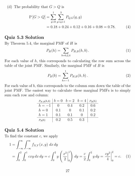
(d) The probability that G > Q is
P [G > Q] =1∑q=0
3∑g=q+1
PQ,G(q, g)
= 0.18 + 0.24 + 0.12 + 0.16 + 0.08 = 0.78. (4)
Quiz 5.3 SolutionBy Theorem 5.4, the marginal PMF of H is
PH (h) =∑b=0,2,4
PH,B(h, b) . (1)
For each value of h, this corresponds to calculating the row sum across thetable of the joint PMF. Similarly, the marginal PMF of B is
PB(b) =1∑
h=−1
PH,B(h, b) . (2)
For each value of b, this corresponds to the column sum down the table of thejoint PMF. The easiest way to calculate these marginal PMFs is to simplysum each row and column:
PH,B(h,b) b = 0 b = 2 b = 4 PH(h)
h = −1 0 0.4 0.2 0.6h = 0 0.1 0 0.1 0.2h = 1 0.1 0.1 0 0.2PB(b) 0.2 0.5 0.3
Quiz 5.4 SolutionTo find the constant c, we apply
1 =
∫ ∞−∞
∫ ∞−∞
fX,Y (x, y) dx dy
=
∫ 2
0
∫ 1
0
cxy dx dy = c
∫ 2
0
y
(x2
2
∣∣∣∣10
)dy =
c
2
∫ 2
0
y dy =cy2
4
∣∣∣∣20
= c. (1)
27
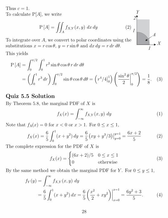
Thus c = 1.To calculate P[A], we write
P [A] =
∫∫A
fX,Y (x, y) dx dy (2)
To integrate over A, we convert to polar coordinates using thesubstitutions x = r cos θ, y = r sin θ and dx dy = r dr dθ.
Y
X
1
1
2
A
This yields
P [A] =
∫ π/2
0
∫ 1
0
r2 sin θ cos θ r dr dθ
=
(∫ 1
0
r3 dr
)∫ π/2
0
sin θ cos θ dθ =(r4/4
∣∣10
)( sin2 θ
2
∣∣∣∣π/20
)=
1
8. (3)
Quiz 5.5 SolutionBy Theorem 5.8, the marginal PDF of X is
fX (x) =
∫ ∞−∞
fX,Y (x, y) dy (1)
Note that fX(x) = 0 for x < 0 or x > 1. For 0 ≤ x ≤ 1,
fX (x) =6
5
∫ 1
0
(x+ y2) dy =6
5
(xy + y3/3
)∣∣y=1
y=0=
6x+ 2
5(2)
The complete expression for the PDF of X is
fX (x) =
{(6x+ 2)/5 0 ≤ x ≤ 1
0 otherwise(3)
By the same method we obtain the marginal PDF for Y . For 0 ≤ y ≤ 1,
fY (y) =
∫ ∞−∞
fX,Y (x, y) dy
=6
5
∫ 1
0
(x+ y2) dx =6
5
(x2
2+ xy2
)∣∣∣∣x=1
x=0
=6y2 + 3
5. (4)
28
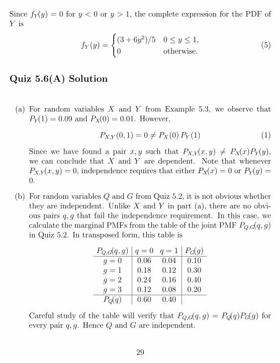
Since fY(y) = 0 for y < 0 or y > 1, the complete expression for the PDF ofY is
fY (y) =
{(3 + 6y2)/5 0 ≤ y ≤ 1,
0 otherwise.(5)
Quiz 5.6(A) Solution
(a) For random variables X and Y from Example 5.3, we observe thatPY(1) = 0.09 and PX(0) = 0.01. However,
PX,Y (0, 1) = 0 6= PX (0)PY (1) (1)
Since we have found a pair x, y such that PX,Y(x, y) 6= PX(x)PY(y),we can conclude that X and Y are dependent. Note that wheneverPX,Y(x, y) = 0, independence requires that either PX(x) = 0 or PY(y) =0.
(b) For random variables Q and G from Quiz 5.2, it is not obvious whetherthey are independent. Unlike X and Y in part (a), there are no obvi-ous pairs q, g that fail the independence requirement. In this case, wecalculate the marginal PMFs from the table of the joint PMF PQ,G(q, g)in Quiz 5.2. In transposed form, this table is
PQ,G(q, g) q = 0 q = 1 PG(g)g = 0 0.06 0.04 0.10g = 1 0.18 0.12 0.30g = 2 0.24 0.16 0.40g = 3 0.12 0.08 0.20PQ(q) 0.60 0.40
Careful study of the table will verify that PQ,G(q, g) = PQ(q)PG(g) forevery pair q, g. Hence Q and G are independent.
29
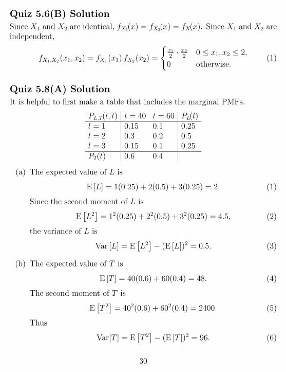
Quiz 5.6(B) SolutionSince X1 and X2 are identical, fX1(x) = fX2(x) = fX(x). Since X1 and X2 areindependent,
fX1,X2(x1, x2) = fX1(x1) fX2(x2) =
{x12· x2
20 ≤ x1, x2 ≤ 2,
0 otherwise.(1)
Quiz 5.8(A) SolutionIt is helpful to first make a table that includes the marginal PMFs.
PL,T(l, t) t = 40 t = 60 PL(l)l = 1 0.15 0.1 0.25l = 2 0.3 0.2 0.5l = 3 0.15 0.1 0.25PT(t) 0.6 0.4
(a) The expected value of L is
E [L] = 1(0.25) + 2(0.5) + 3(0.25) = 2. (1)
Since the second moment of L is
E[L2]
= 12(0.25) + 22(0.5) + 32(0.25) = 4.5, (2)
the variance of L is
Var [L] = E[L2]− (E [L])2 = 0.5. (3)
(b) The expected value of T is
E [T ] = 40(0.6) + 60(0.4) = 48. (4)
The second moment of T is
E[T 2]
= 402(0.6) + 602(0.4) = 2400. (5)
Thus
Var[T ] = E[T 2]− (E [T ])2 = 96. (6)
30
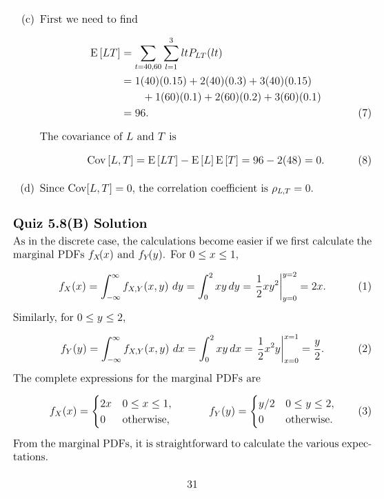
(c) First we need to find
E [LT ] =∑
t=40,60
3∑l=1
ltPLT (lt)
= 1(40)(0.15) + 2(40)(0.3) + 3(40)(0.15)
+ 1(60)(0.1) + 2(60)(0.2) + 3(60)(0.1)
= 96. (7)
The covariance of L and T is
Cov [L, T ] = E [LT ]− E [L] E [T ] = 96− 2(48) = 0. (8)
(d) Since Cov[L, T ] = 0, the correlation coefficient is ρL,T = 0.
Quiz 5.8(B) Solution
As in the discrete case, the calculations become easier if we first calculate themarginal PDFs fX(x) and fY(y). For 0 ≤ x ≤ 1,
fX (x) =
∫ ∞−∞
fX,Y (x, y) dy =
∫ 2
0
xy dy =1
2xy2∣∣∣∣y=2
y=0
= 2x. (1)
Similarly, for 0 ≤ y ≤ 2,
fY (y) =
∫ ∞−∞
fX,Y (x, y) dx =
∫ 2
0
xy dx =1
2x2y
∣∣∣∣x=1
x=0
=y
2. (2)
The complete expressions for the marginal PDFs are
fX (x) =
{2x 0 ≤ x ≤ 1,
0 otherwise,fY (y) =
{y/2 0 ≤ y ≤ 2,
0 otherwise.(3)
From the marginal PDFs, it is straightforward to calculate the various expec-tations.
31
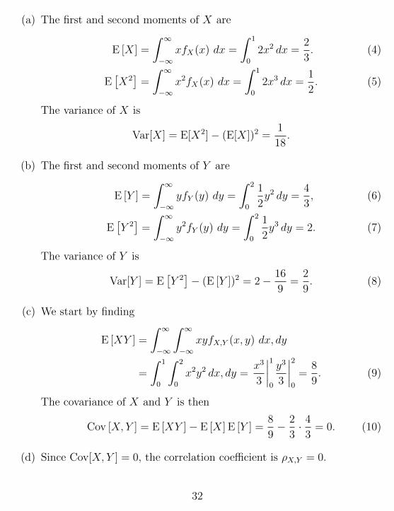
(a) The first and second moments of X are
E [X] =
∫ ∞−∞
xfX (x) dx =
∫ 1
0
2x2 dx =2
3. (4)
E[X2]
=
∫ ∞−∞
x2fX (x) dx =
∫ 1
0
2x3 dx =1
2. (5)
The variance of X is
Var[X] = E[X2]− (E[X])2 =1
18.
(b) The first and second moments of Y are
E [Y ] =
∫ ∞−∞
yfY (y) dy =
∫ 2
0
1
2y2 dy =
4
3, (6)
E[Y 2]
=
∫ ∞−∞
y2fY (y) dy =
∫ 2
0
1
2y3 dy = 2. (7)
The variance of Y is
Var[Y ] = E[Y 2]− (E [Y ])2 = 2− 16
9=
2
9. (8)
(c) We start by finding
E [XY ] =
∫ ∞−∞
∫ ∞−∞
xyfX,Y (x, y) dx, dy
=
∫ 1
0
∫ 2
0
x2y2 dx, dy =x3
3
∣∣∣∣10
y3
3
∣∣∣∣20
=8
9. (9)
The covariance of X and Y is then
Cov [X, Y ] = E [XY ]− E [X] E [Y ] =8
9− 2
3· 4
3= 0. (10)
(d) Since Cov[X, Y ] = 0, the correlation coefficient is ρX,Y = 0.
32
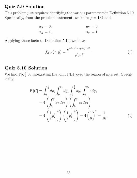
Quiz 5.9 Solution
This problem just requires identifying the various parameters in Definition 5.10.Specifically, from the problem statement, we know ρ = 1/2 and
µX = 0, µY = 0,
σX = 1, σY = 1.
Applying these facts to Definition 5.10, we have
fX,Y (x, y) =e−2(x
2−xy+y2)/3√
3π2. (1)
Quiz 5.10 Solution
We find P[C] by integrating the joint PDF over the region of interest. Specif-ically,
P [C] =
∫ 12
0
dy2
∫ y2
0
dy1
∫ 12
0
dy4
∫ y4
0
4dy3
= 4
(∫ 12
0
y2 dy2
)(∫ 12
0
y4 dy4
)
= 4
(1
2y22
∣∣∣∣ 120
)(1
2y24
∣∣∣∣ 120
)= 4
(1
8
)2
=1
16. (1)
33

Quiz 6.2 Solution
Since Y =√X, the fact that X is nonegative implies Y is non-negative. This
implies FY(y) = 0 for y < 0. For y ≥ 0, we find
FY (y) = P[√
X ≤ y]
= P[X ≤ y2
]= FX
(y2). (1)
For x ≥ 0, FX(x) = 1− e−λx. Thus,
FY (y) =
{1− e−λy2 y ≥ 0
0 otherwise(2)
By taking the derivative with respect to y, it follows that the PDF of Y is
fY (y) =
{2λye−λy
2y ≥ 0
0 otherwise(3)
In comparing this result to the Rayleigh PDF given in Appendix A, we observethat Y is a Rayleigh (a) random variable with a =
√2λ.
Quiz 6.3 Solution
(a) Since X is always nonnegative, FX(x) = 0 for x < 0. Also, FX(x) = 1for x ≥ 2 since its always true that x ≤ 2. Lastly, for 0 ≤ x ≤ 2,
FX (x) =
∫ x
−∞fX (y) dy =
∫ x
0
(1− y/2) dy = x− x2/4. (1)
The complete CDF of X is
−1 0 1 2 30
0.5
1
x
FX(x
)
FX (x) =
0 x < 0,
x− x2/4 0 ≤ x ≤ 2,
1 x > 2.
(2)
34
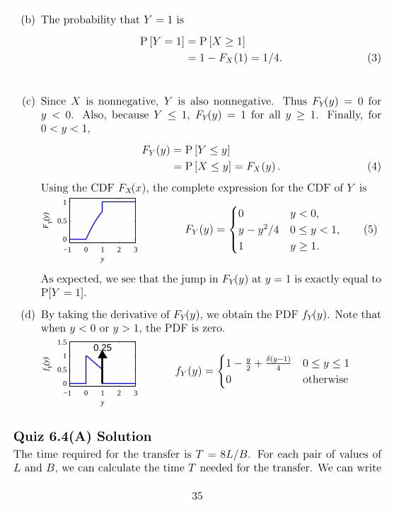
(b) The probability that Y = 1 is
P [Y = 1] = P [X ≥ 1]
= 1− FX (1) = 1/4. (3)
(c) Since X is nonnegative, Y is also nonnegative. Thus FY(y) = 0 fory < 0. Also, because Y ≤ 1, FY(y) = 1 for all y ≥ 1. Finally, for0 < y < 1,
FY (y) = P [Y ≤ y]
= P [X ≤ y] = FX (y) . (4)
Using the CDF FX(x), the complete expression for the CDF of Y is
−1 0 1 2 30
0.5
1
y
FY(y
)
FY (y) =
0 y < 0,
y − y2/4 0 ≤ y < 1,
1 y ≥ 1.
(5)
As expected, we see that the jump in FY(y) at y = 1 is exactly equal toP[Y = 1].
(d) By taking the derivative of FY(y), we obtain the PDF fY(y). Note thatwhen y < 0 or y > 1, the PDF is zero.
−1 0 1 2 30
0.5
1
1.5
y
f Y(y
)
0.25
fY (y) =
{1− y
2+ δ(y−1)
40 ≤ y ≤ 1
0 otherwise
Quiz 6.4(A) SolutionThe time required for the transfer is T = 8L/B. For each pair of values ofL and B, we can calculate the time T needed for the transfer. We can write
35
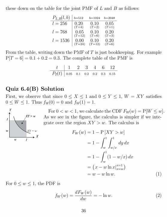
these down on the table for the joint PMF of L and B as follows:
PL,B(l, b) b=512 b=1024 b=2048
l = 256 0.20(T=4)
0.10(T=2)
0.05(T=1)
l = 768 0.05(T=12)
0.10(T=6)
0.20(T=3)
l = 1536 0.00(T=24)
0.10(T=12)
0.20(T=6)
From the table, writing down the PMF of T is just bookkeeping. For exampleP[T = 6] = 0.1 + 0.2 = 0.3. The complete table of the PMF is
t 1 2 3 4 6 12PT(t) 0.05 0.1 0.2 0.2 0.3 0.15
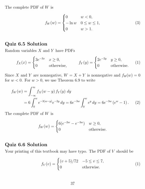
Quiz 6.4(B) Solution
First, we observe that since 0 ≤ X ≤ 1 and 0 ≤ Y ≤ 1, W = XY satisfies0 ≤ W ≤ 1. Thus fW(0) = 0 and fW(1) = 1.
Y
X
1
1
XY > w
w
w XY = w
Y
X
1
1
XY > w
w
w
For 0 < w < 1, we calculate the CDF FW(w) = P[W ≤ w].As we see in the figure, the calculus is simpler if we inte-grate over the region XY > w. The calculus is
FW (w) = 1− P [XY > w]
= 1−∫ 1
w
∫ 1
w/x
dy dx
= 1−∫ 1
w
(1− w/x) dx
=(x− w lnx|x=1
x=w
)= w − w lnw. (1)
For 0 ≤ w ≤ 1, the PDF is
fW (w) =dFW (w)
dw= − lnw. (2)
36
The complete PDF of W is
fW (w) =
0 w < 0,
− lnw 0 ≤ w ≤ 1,
0 w > 1.
(3)
Quiz 6.5 Solution
Random variables X and Y have PDFs
fX (x) =
{3e−3x x ≥ 0,
0 otherwise,fY (y) =
{2e−2y y ≥ 0,
0 otherwise.(1)
Since X and Y are nonnegative, W = X + Y is nonnegative and fW(w) = 0for w < 0. For w > 0, we use Theorem 6.9 to write
fW (w) =
∫ ∞−∞
fX (w − y) fY (y) dy
= 6
∫ w
0
e−3(w−y)e−2y dy = 6e−3w∫ w
0
ey dy = 6e−3w (ew − 1) . (2)
The complete PDF of W is
fW (w) =
{6(e−2w − e−3w) w ≥ 0,
0 otherwise.
Quiz 6.6 Solution
Your printing of this textbook may have typo. The PDF of V should be
fV (v) =
{(v + 5)/72 −5 ≤ v ≤ 7,
0 otherwise.(1)
37
First we find the corresponding CDF FV(v). For −5 ≤ v ≤ 7,
FV (v) =
∫ v
−∞fV (u) du =
∫ v
−5
u+ 5
72du (2)
=(u+ 5)2
144
∣∣∣∣v−5
=(v + 5)2
144. (3)
The complete CDF of V is
FV (v) =
0 v < −5,
(v + 5)2/144 −5 ≤ v ≤ 7,
1 v > 7.
(4)
Now that we found the CDF FV(v), we can use Theorem 6.5. Over the interval−5 ≤ v ≤ 7, we find the inverse of the CDF by solving
u = FV (v) =(v + 5)2
144(5)
for v as a function of u. This yields v = 12√u−5. Thus, when U is a uniform
(0, 1) random variable, the function
V = 12√U − 5 (6)
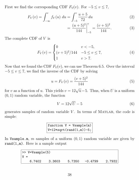
generates samples of random variable V . In terms of Matlab, the code issimple:
function V = Vsample(m)
V=12*sqrt(rand(1,m))-5;
In Vsample.m, m samples of a uniform (0, 1) random variable are given byrand(1,m). Here is a sample output
>> V=Vsample(5)
V =
6.7402 3.3603 5.7350 -0.4799 2.7932
38
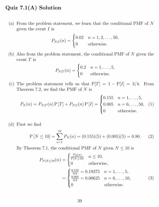
Quiz 7.1(A) Solution
(a) From the problem statement, we learn that the conditional PMF of Ngiven the event I is
PN |I (n) =
{0.02 n = 1, 2, . . . , 50,
0 otherwise.
(b) Also from the problem statement, the conditional PMF of N given theevent T is
PN |T (n) =
{0.2 n = 1, . . . , 5,
0 otherwise.
(c) The problem statement tells us that P[T ] = 1 − P[I] = 3/4. FromTheorem 7.2, we find the PMF of N is
PN (n) = PN |T (n) P [T ] + PN |I (n) P [I] =
0.155 n = 1, . . . , 5,
0.005 n = 6, . . . , 50,
0 otherwise.
(1)
(d) First we find
P [N ≤ 10] =10∑n=1
PN (n) = (0.155)(5) + (0.005)(5) = 0.80. (2)
By Theorem 7.1, the conditional PMF of N given N ≤ 10 is
PN |N≤10(n) =
{PN(n)
P[N≤10] n ≤ 10,
0 otherwise,
=
0.1550.8
= 0.19375 n = 1, . . . , 5,0.0050.8
= 0.00625 n = 6, . . . , 10,
0 otherwise.
(3)
39
Quiz 7.1(B) Solution
From the problem statement,
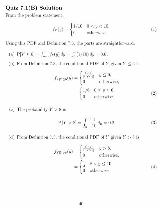
fY (y) =
{1/10 0 < y < 10,
0 otherwise.(1)
Using this PDF and Definition 7.3, the parts are straightforward.
(a) P[Y ≤ 6] =∫ 6
−∞ fY(y) dy =∫ 6
0(1/10) dy = 0.6 .
(b) From Definition 7.3, the conditional PDF of Y given Y ≤ 6 is
fY |Y≤6(y) =
{fY(y)P[Y≤6] y ≤ 6,
0 otherwise,
=
{1/6 0 ≤ y ≤ 6,
0 otherwise.(2)
(c) The probability Y > 8 is
P [Y > 8] =
∫ 10
8
1
10dy = 0.2. (3)
(d) From Definition 7.3, the conditional PDF of Y given Y > 8 is
fY |Y >8(y) =
{fY(y)P[Y >8]
y > 8,
0 otherwise,
=
{12
8 < y ≤ 10,
0 otherwise.(4)
40

Quiz 7.2(A) Solution
We refer to the solution of Quiz 7.1(A) for PN |N≤10(n).
(a) Given PN |N≤10(n), calculating a conditional expected value is the sameas for any other expected value except we use the conditional PMF.
E [N |N ≤ 10] =∑n
nPN |N≤10(n)
=5∑
n=1
0.19375n+10∑n=6
0.00625n = 3.15625. (1)
(b) For the conditional variance, we first find the conditional second mo-ment
E[N2|N ≤ 10
]=∑n
n2PN |N≤10(n)
=5∑
n=1
0.19375n2 +10∑n=6
0.00625n2
= 0.19375(55) + 0.00625(330) = 12.719. (2)
The conditional variance is
Var[N |N ≤ 10] = E[N2|N ≤ 10
]− (E [N |N ≤ 10])2
= 12.719− (3.156)2 = 2.757. (3)
Quiz 7.2(B) Solution
We refer to the solution of Quiz 7.1(B) for the conditional PDFs fY |Y≤6(y)and fY |Y >8(y).
(a) From fY |Y≤6(y), the conditional expectation is
E [Y |Y ≤ 6] =
∫ ∞−∞
yfY |Y≤6(y) dy =
∫ 6
0
y
6dy = 3. (1)
41
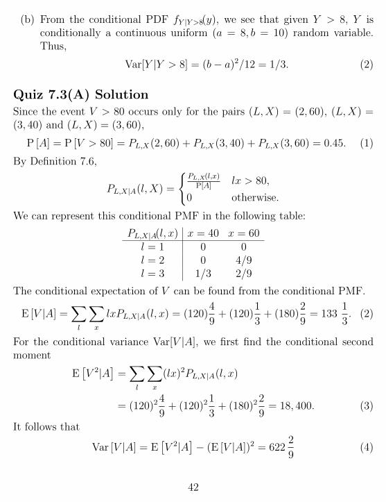
(b) From the conditional PDF fY |Y >8(y), we see that given Y > 8, Y isconditionally a continuous uniform (a = 8, b = 10) random variable.Thus,
Var[Y |Y > 8] = (b− a)2/12 = 1/3. (2)
Quiz 7.3(A) SolutionSince the event V > 80 occurs only for the pairs (L,X) = (2, 60), (L,X) =(3, 40) and (L,X) = (3, 60),
P [A] = P [V > 80] = PL,X (2, 60) + PL,X (3, 40) + PL,X (3, 60) = 0.45. (1)
By Definition 7.6,
PL,X|A(l, X) =
{PL,X(l,x)
P[A]lx > 80,
0 otherwise.
We can represent this conditional PMF in the following table:
PL,X|A(l, x) x = 40 x = 60l = 1 0 0l = 2 0 4/9l = 3 1/3 2/9
The conditional expectation of V can be found from the conditional PMF.
E [V |A] =∑l
∑x
lxPL,X|A(l, x) = (120)4
9+ (120)
1
3+ (180)
2
9= 133
1
3. (2)
For the conditional variance Var[V |A], we first find the conditional secondmoment
E[V 2|A
]=∑l
∑x
(lx)2PL,X|A(l, x)
= (120)24
9+ (120)2
1
3+ (180)2
2
9= 18, 400. (3)
It follows that
Var [V |A] = E[V 2|A
]− (E [V |A])2 = 622
2
9(4)
42
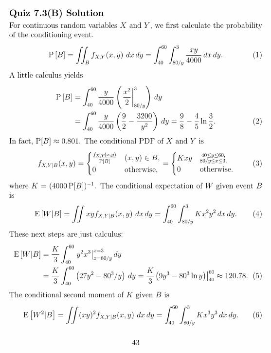
Quiz 7.3(B) Solution
For continuous random variables X and Y , we first calculate the probabilityof the conditioning event.
P [B] =
∫∫B
fX,Y (x, y) dx dy =
∫ 60
40
∫ 3
80/y
xy
4000dx dy. (1)
A little calculus yields
P [B] =
∫ 60
40
y
4000
(x2
2
∣∣∣∣380/y
)dy
=
∫ 60
40
y
4000
(9
2− 3200
y2
)dy =
9
8− 4
5ln
3
2. (2)
In fact, P[B] ≈ 0.801. The conditional PDF of X and Y is
fX,Y |B(x, y) =
{fX,Y(x,y)
P[B](x, y) ∈ B,
0 otherwise,=
{Kxy 40≤y≤60,
80/y≤x≤3,
0 otherwise.(3)
where K = (4000 P[B])−1. The conditional expectation of W given event Bis
E [W |B] =
∫∫xyfX,Y |B(x, y) dx dy =
∫ 60
40
∫ 3
80/y
Kx2y2 dx dy. (4)
These next steps are just calculus:
E [W |B] =K
3
∫ 60
40
y2x3∣∣x=3
x=80/ydy
=K
3
∫ 60
40
(27y2 − 803/y
)dy =
K
3
(9y3 − 803 ln y
)∣∣6040≈ 120.78. (5)
The conditional second moment of K given B is
E[W 2|B
]=
∫∫(xy)2fX,Y |B(x, y) dx dy =
∫ 60
40
∫ 3
80/y
Kx3y3 dx dy. (6)
43
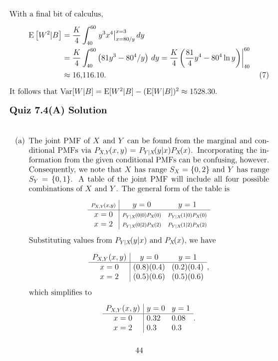
With a final bit of calculus,
E[W 2|B
]=K
4
∫ 60
40
y3x4∣∣x=3
x=80/ydy
=K
4
∫ 60
40
(81y3 − 804/y
)dy =
K
4
(81
4y4 − 804 ln y
)∣∣∣∣6040
≈ 16,116.10. (7)
It follows that Var[W |B] = E[W 2|B]− (E[W |B])2 ≈ 1528.30.
Quiz 7.4(A) Solution
(a) The joint PMF of X and Y can be found from the marginal and con-ditional PMFs via PX,Y(x, y) = PY |X(y|x)PX(x). Incorporating the in-formation from the given conditional PMFs can be confusing, however.Consequently, we note that X has range SX = {0, 2} and Y has rangeSY = {0, 1}. A table of the joint PMF will include all four possiblecombinations of X and Y . The general form of the table is
PX,Y(x,y) y = 0 y = 1x = 0 PY |X(0|0)PX(0) PY |X(1|0)PX(0)
x = 2 PY |X(0|2)PX(2) PY |X(1|2)PX(2)
Substituting values from PY |X(y|x) and PX(x), we have
PX,Y (x, y) y = 0 y = 1x = 0 (0.8)(0.4) (0.2)(0.4)x = 2 (0.5)(0.6) (0.5)(0.6)
,
which simplifies to
PX,Y (x, y) y = 0 y = 1x = 0 0.32 0.08x = 2 0.3 0.3
.
44
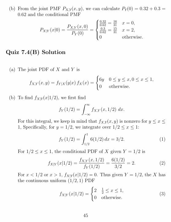
(b) From the joint PMF PX,Y(x, y), we can calculate PY(0) = 0.32 + 0.3 =0.62 and the conditional PMF
PX|Y (x|0) =PX,Y (x, 0)
PY (0)=
0.320.62
= 1631
x = 0,0.30.62
= 1531
x = 2,
0 otherwise.
Quiz 7.4(B) Solution
(a) The joint PDF of X and Y is
fX,Y (x, y) = fY |X (y|x) fX (x) =
{6y 0 ≤ y ≤ x, 0 ≤ x ≤ 1,
0 otherwise.
(b) To find fX|Y(x|1/2), we first find
fY (1/2) =
∫ ∞−∞
fX,Y (x, 1/2) dx.
For this integral, we keep in mind that fX,Y(x, y) is nonzero for y ≤ x ≤1, Specifically, for y = 1/2, we integrate over 1/2 ≤ x ≤ 1:
fY (1/2) =
∫ 1
1/2
6(1/2) dx = 3/2. (1)
For 1/2 ≤ x ≤ 1, the conditional PDF of X given Y = 1/2 is
fX|Y (x|1/2) =fX,Y (x, 1/2)
fY (1/2)=
6(1/2)
3/2= 2. (2)
For x < 1/2 or x > 1, fX|Y(x|1/2) = 0. Thus given Y = 1/2, the X hasthe continuous uniform (1/2, 1) PDF
fX|Y (x|1/2) =
{2 1
2≤ x ≤ 1,
0 otherwise.(3)
45
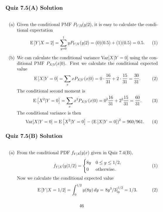
Quiz 7.5(A) Solution
(a) Given the conditional PMF PY |X(y|2), it is easy to calculate the condi-tional expectation
E [Y |X = 2] =1∑y=0
yPY |X (y|2) = (0)(0.5) + (1)(0.5) = 0.5. (1)
(b) We can calculate the conditional variance Var[X|Y = 0] using the con-ditional PMF PX|Y(x|0). First we calculate the conditional expectedvalue
E [X|Y = 0] =∑x
xPX|Y (x|0) = 0 · 16
31+ 2 · 15
31=
30
31. (2)
The conditional second moment is
E[X2|Y = 0
]=∑x
x2PX|Y (x|0) = 0216
31+ 2215
31=
60
31. (3)
The conditional variance is then
Var[X|Y = 0] = E[X2|Y = 0
]− (E [X|Y = 0])2 = 960/961. (4)
Quiz 7.5(B) Solution
(a) From the conditional PDF fY |X(y|x) given in Quiz 7.4(B),
fY |X (y|1/2) =
{8y 0 ≤ y ≤ 1/2,
0 otherwise.(1)
Now we calculate the conditional expected value
E [Y |X = 1/2] =
∫ 1/2
0
y(8y) dy = 8y3/3∣∣1/20
= 1/3. (2)
46
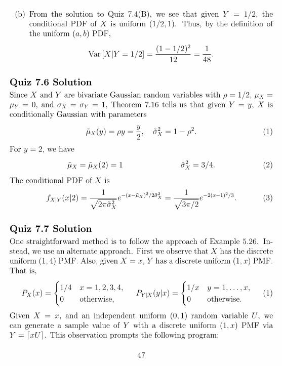
(b) From the solution to Quiz 7.4(B), we see that given Y = 1/2, theconditional PDF of X is uniform (1/2, 1). Thus, by the definition ofthe uniform (a, b) PDF,
Var [X|Y = 1/2] =(1− 1/2)2
12=
1
48.
Quiz 7.6 Solution
Since X and Y are bivariate Gaussian random variables with ρ = 1/2, µX =µY = 0, and σX = σY = 1, Theorem 7.16 tells us that given Y = y, X isconditionally Gaussian with parameters
µX(y) = ρy =y
2, σ2
X = 1− ρ2. (1)
For y = 2, we have
µX = µX(2) = 1 σ2X = 3/4. (2)
The conditional PDF of X is
fX|Y (x|2) =1√
2πσ2X
e−(x−µX)2/2σ2X =
1√3π/2
e−2(x−1)2/3. (3)
Quiz 7.7 Solution
One straightforward method is to follow the approach of Example 5.26. In-stead, we use an alternate approach. First we observe that X has the discreteuniform (1, 4) PMF. Also, given X = x, Y has a discrete uniform (1, x) PMF.That is,
PX (x) =
{1/4 x = 1, 2, 3, 4,
0 otherwise,PY |X (y|x) =
{1/x y = 1, . . . , x,
0 otherwise.(1)
Given X = x, and an independent uniform (0, 1) random variable U , wecan generate a sample value of Y with a discrete uniform (1, x) PMF viaY = dxUe. This observation prompts the following program:
47

function xy=dtrianglerv(m)
sx=[1;2;3;4];
px=0.25*ones(4,1);
x=finiterv(sx,px,m);
y=ceil(x.*rand(m,1));
xy=[x’;y’];
48
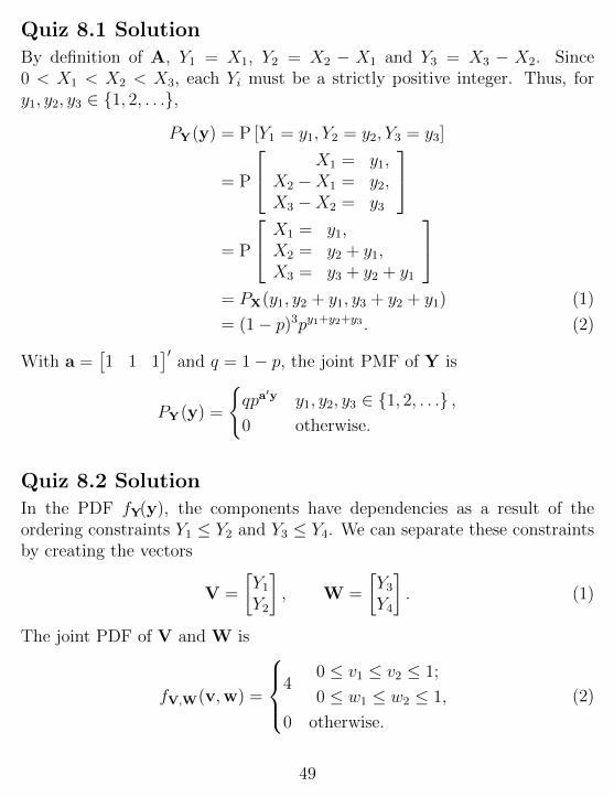
Quiz 8.1 SolutionBy definition of A, Y1 = X1, Y2 = X2 − X1 and Y3 = X3 − X2. Since0 < X1 < X2 < X3, each Yi must be a strictly positive integer. Thus, fory1, y2, y3 ∈ {1, 2, . . .},
PY(y) = P [Y1 = y1, Y2 = y2, Y3 = y3]
= P
X1 = y1,X2 −X1 = y2,X3 −X2 = y3
= P
X1 = y1,X2 = y2 + y1,X3 = y3 + y2 + y1
= PX(y1, y2 + y1, y3 + y2 + y1) (1)
= (1− p)3py1+y2+y3 . (2)
With a =[1 1 1
]′and q = 1− p, the joint PMF of Y is
PY(y) =
{qpa
′y y1, y2, y3 ∈ {1, 2, . . .} ,0 otherwise.
Quiz 8.2 SolutionIn the PDF fY(y), the components have dependencies as a result of theordering constraints Y1 ≤ Y2 and Y3 ≤ Y4. We can separate these constraintsby creating the vectors
V =
[Y1Y2
], W =
[Y3Y4
]. (1)
The joint PDF of V and W is
fV,W(v,w) =
40 ≤ v1 ≤ v2 ≤ 1;
0 ≤ w1 ≤ w2 ≤ 1,
0 otherwise.
(2)
49
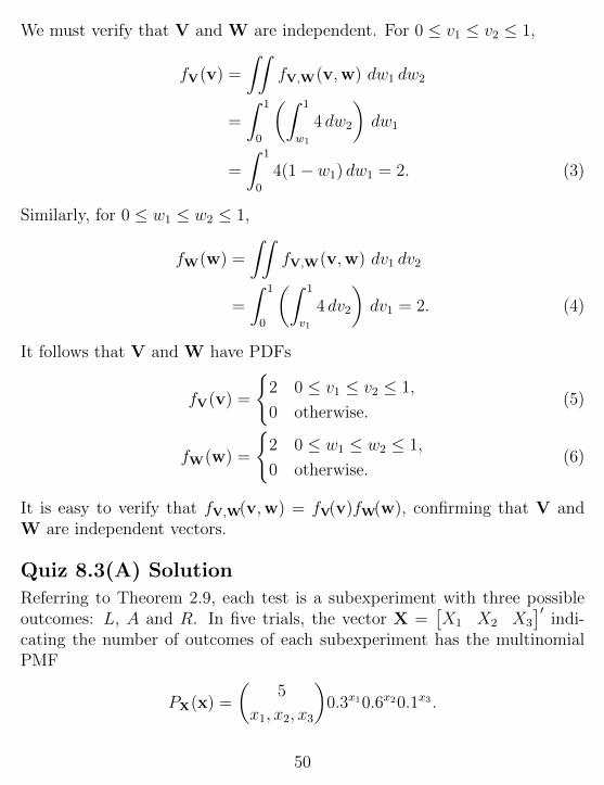
We must verify that V and W are independent. For 0 ≤ v1 ≤ v2 ≤ 1,
fV(v) =
∫∫fV,W(v,w) dw1 dw2
=
∫ 1
0
(∫ 1
w1
4 dw2
)dw1
=
∫ 1
0
4(1− w1) dw1 = 2. (3)
Similarly, for 0 ≤ w1 ≤ w2 ≤ 1,
fW(w) =
∫∫fV,W(v,w) dv1 dv2
=
∫ 1
0
(∫ 1
v1
4 dv2
)dv1 = 2. (4)
It follows that V and W have PDFs
fV(v) =
{2 0 ≤ v1 ≤ v2 ≤ 1,
0 otherwise.(5)
fW(w) =
{2 0 ≤ w1 ≤ w2 ≤ 1,
0 otherwise.(6)
It is easy to verify that fV,W(v,w) = fV(v)fW(w), confirming that V andW are independent vectors.
Quiz 8.3(A) Solution
Referring to Theorem 2.9, each test is a subexperiment with three possibleoutcomes: L, A and R. In five trials, the vector X =
[X1 X2 X3
]′indi-
cating the number of outcomes of each subexperiment has the multinomialPMF
PX(x) =
(5
x1, x2, x3
)0.3x10.6x20.1x3 .
50
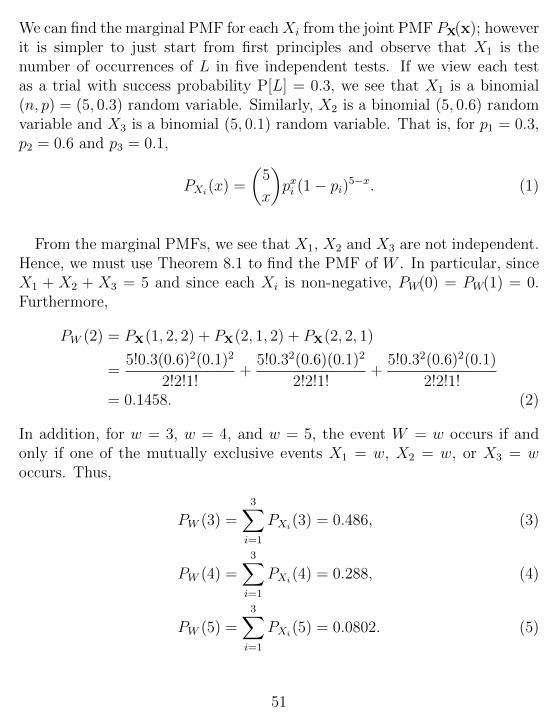
We can find the marginal PMF for eachXi from the joint PMF PX(x); howeverit is simpler to just start from first principles and observe that X1 is thenumber of occurrences of L in five independent tests. If we view each testas a trial with success probability P[L] = 0.3, we see that X1 is a binomial(n, p) = (5, 0.3) random variable. Similarly, X2 is a binomial (5, 0.6) randomvariable and X3 is a binomial (5, 0.1) random variable. That is, for p1 = 0.3,p2 = 0.6 and p3 = 0.1,
PXi(x) =
(5
x
)pxi (1− pi)5−x. (1)
From the marginal PMFs, we see that X1, X2 and X3 are not independent.Hence, we must use Theorem 8.1 to find the PMF of W . In particular, sinceX1 + X2 + X3 = 5 and since each Xi is non-negative, PW(0) = PW(1) = 0.Furthermore,
PW (2) = PX(1, 2, 2) + PX(2, 1, 2) + PX(2, 2, 1)
=5!0.3(0.6)2(0.1)2
2!2!1!+
5!0.32(0.6)(0.1)2
2!2!1!+
5!0.32(0.6)2(0.1)
2!2!1!= 0.1458. (2)
In addition, for w = 3, w = 4, and w = 5, the event W = w occurs if andonly if one of the mutually exclusive events X1 = w, X2 = w, or X3 = woccurs. Thus,
PW (3) =3∑i=1
PXi(3) = 0.486, (3)
PW (4) =3∑i=1
PXi(4) = 0.288, (4)
PW (5) =3∑i=1
PXi(5) = 0.0802. (5)
51
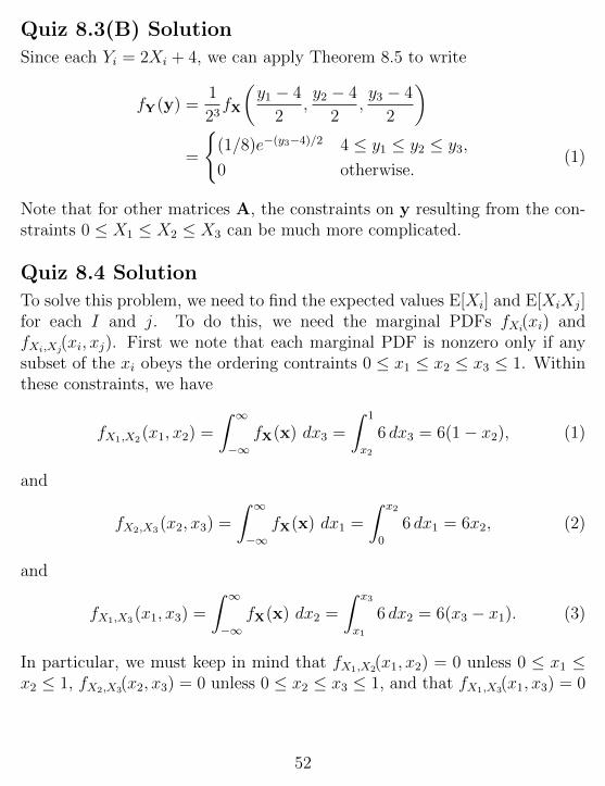
Quiz 8.3(B) Solution
Since each Yi = 2Xi + 4, we can apply Theorem 8.5 to write
fY(y) =1
23fX
(y1 − 4
2,y2 − 4
2,y3 − 4
2
)=
{(1/8)e−(y3−4)/2 4 ≤ y1 ≤ y2 ≤ y3,
0 otherwise.(1)
Note that for other matrices A, the constraints on y resulting from the con-straints 0 ≤ X1 ≤ X2 ≤ X3 can be much more complicated.
Quiz 8.4 Solution
To solve this problem, we need to find the expected values E[Xi] and E[XiXj]for each I and j. To do this, we need the marginal PDFs fXi(xi) andfXi,Xj(xi, xj). First we note that each marginal PDF is nonzero only if anysubset of the xi obeys the ordering contraints 0 ≤ x1 ≤ x2 ≤ x3 ≤ 1. Withinthese constraints, we have
fX1,X2(x1, x2) =
∫ ∞−∞
fX(x) dx3 =
∫ 1
x2
6 dx3 = 6(1− x2), (1)
and
fX2,X3(x2, x3) =
∫ ∞−∞
fX(x) dx1 =
∫ x2
0
6 dx1 = 6x2, (2)
and
fX1,X3(x1, x3) =
∫ ∞−∞
fX(x) dx2 =
∫ x3
x1
6 dx2 = 6(x3 − x1). (3)
In particular, we must keep in mind that fX1,X2(x1, x2) = 0 unless 0 ≤ x1 ≤x2 ≤ 1, fX2,X3(x2, x3) = 0 unless 0 ≤ x2 ≤ x3 ≤ 1, and that fX1,X3(x1, x3) = 0
52
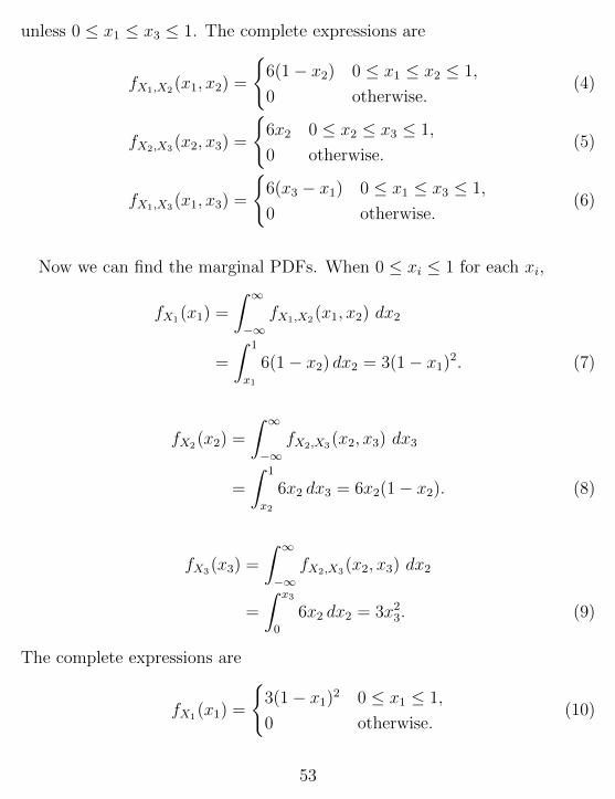
unless 0 ≤ x1 ≤ x3 ≤ 1. The complete expressions are
fX1,X2(x1, x2) =
{6(1− x2) 0 ≤ x1 ≤ x2 ≤ 1,
0 otherwise.(4)
fX2,X3(x2, x3) =
{6x2 0 ≤ x2 ≤ x3 ≤ 1,
0 otherwise.(5)
fX1,X3(x1, x3) =
{6(x3 − x1) 0 ≤ x1 ≤ x3 ≤ 1,
0 otherwise.(6)
Now we can find the marginal PDFs. When 0 ≤ xi ≤ 1 for each xi,
fX1(x1) =
∫ ∞−∞
fX1,X2(x1, x2) dx2
=
∫ 1
x1
6(1− x2) dx2 = 3(1− x1)2. (7)
fX2(x2) =
∫ ∞−∞
fX2,X3(x2, x3) dx3
=
∫ 1
x2
6x2 dx3 = 6x2(1− x2). (8)
fX3(x3) =
∫ ∞−∞
fX2,X3(x2, x3) dx2
=
∫ x3
0
6x2 dx2 = 3x23. (9)
The complete expressions are
fX1(x1) =
{3(1− x1)2 0 ≤ x1 ≤ 1,
0 otherwise.(10)
53
fX2(x2) =
{6x2(1− x2) 0 ≤ x2 ≤ 1,
0 otherwise.(11)
fX3(x3) =
{3x23 0 ≤ x3 ≤ 1,
0 otherwise.(12)
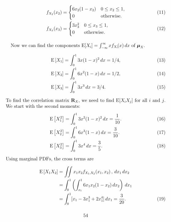
Now we can find the components E[Xi] =∫∞−∞ xfXi(x) dx of µX .
E [X1] =
∫ 1
0
3x(1− x)2 dx = 1/4, (13)
E [X2] =
∫ 1
0
6x2(1− x) dx = 1/2, (14)
E [X3] =
∫ 1
0
3x3 dx = 3/4. (15)
To find the correlation matrix RX , we need to find E[XiXj] for all i and j.We start with the second moments:
E[X2
1
]=
∫ 1
0
3x2(1− x)2 dx =1
10. (16)
E[X2
2
]=
∫ 1
0
6x3(1− x) dx =3
10. (17)
E[X2
3
]=
∫ 1
0
3x4 dx =3
5. (18)
Using marginal PDFs, the cross terms are
E [X1X2] =
∫∫x1x2fX1,X2(x1, x2) , dx1 dx2
=
∫ 1
0
(∫ 1
x1
6x1x2(1− x2) dx2)dx1
=
∫ 1
0
[x1 − 3x31 + 2x41] dx1 =3
20. (19)
54
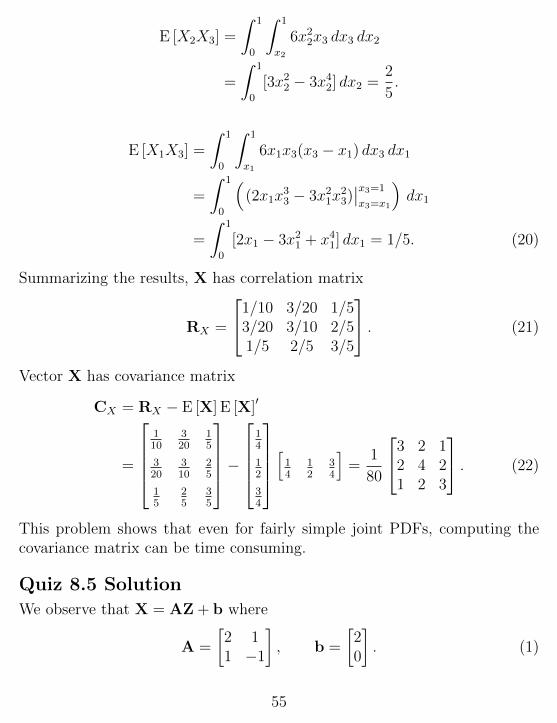
E [X2X3] =
∫ 1
0
∫ 1
x2
6x22x3 dx3 dx2
=
∫ 1
0
[3x22 − 3x42] dx2 =2
5.
E [X1X3] =
∫ 1
0
∫ 1
x1
6x1x3(x3 − x1) dx3 dx1
=
∫ 1
0
((2x1x
33 − 3x21x
23)∣∣x3=1
x3=x1
)dx1
=
∫ 1
0
[2x1 − 3x21 + x41] dx1 = 1/5. (20)
Summarizing the results, X has correlation matrix
RX =
1/10 3/20 1/53/20 3/10 2/51/5 2/5 3/5
. (21)
Vector X has covariance matrix
CX = RX − E [X] E [X]′
=
110
320
15
320
310
25
15
25
35
−
14
12
34
[14 12
34
]=
1
80
3 2 12 4 21 2 3
. (22)
This problem shows that even for fairly simple joint PDFs, computing thecovariance matrix can be time consuming.
Quiz 8.5 Solution
We observe that X = AZ + b where
A =
[2 11 −1
], b =
[20
]. (1)
55
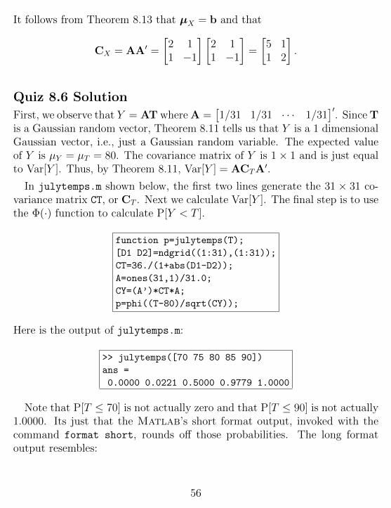
It follows from Theorem 8.13 that µX = b and that
CX = AA′ =
[2 11 −1
] [2 11 −1
]=
[5 11 2
].
Quiz 8.6 Solution
First, we observe that Y = AT where A =[1/31 1/31 · · · 1/31
]′. Since T
is a Gaussian random vector, Theorem 8.11 tells us that Y is a 1 dimensionalGaussian vector, i.e., just a Gaussian random variable. The expected valueof Y is µY = µT = 80. The covariance matrix of Y is 1× 1 and is just equalto Var[Y ]. Thus, by Theorem 8.11, Var[Y ] = ACTA
′.
In julytemps.m shown below, the first two lines generate the 31 × 31 co-variance matrix CT, or CT . Next we calculate Var[Y ]. The final step is to usethe Φ(·) function to calculate P[Y < T ].
function p=julytemps(T);
[D1 D2]=ndgrid((1:31),(1:31));
CT=36./(1+abs(D1-D2));
A=ones(31,1)/31.0;
CY=(A’)*CT*A;
p=phi((T-80)/sqrt(CY));
Here is the output of julytemps.m:
>> julytemps([70 75 80 85 90])
ans =
0.0000 0.0221 0.5000 0.9779 1.0000
Note that P[T ≤ 70] is not actually zero and that P[T ≤ 90] is not actually1.0000. Its just that the Matlab’s short format output, invoked with thecommand format short, rounds off those probabilities. The long formatoutput resembles:
56
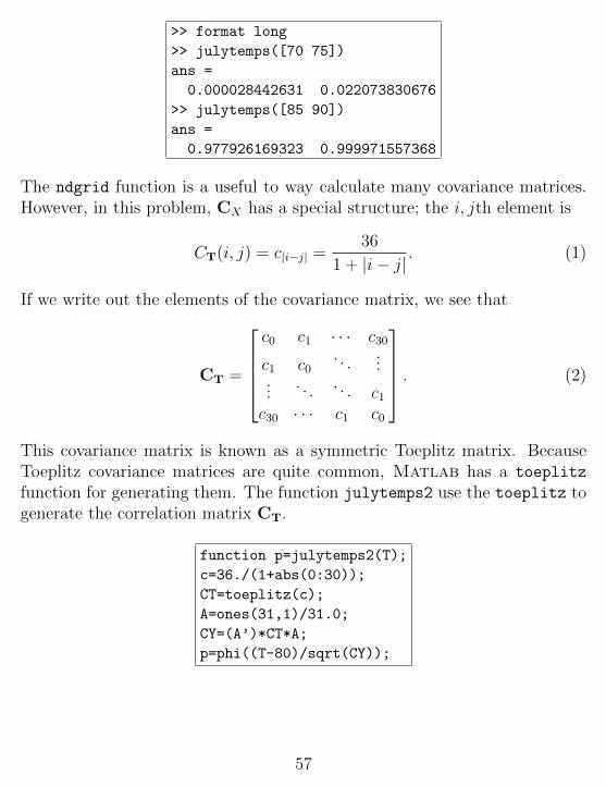
>> format long
>> julytemps([70 75])
ans =
0.000028442631 0.022073830676
>> julytemps([85 90])
ans =
0.977926169323 0.999971557368
The ndgrid function is a useful to way calculate many covariance matrices.However, in this problem, CX has a special structure; the i, jth element is
CT(i, j) = c|i−j| =36
1 + |i− j|. (1)
If we write out the elements of the covariance matrix, we see that
CT =
c0 c1 · · · c30
c1 c0. . .
......
. . . . . . c1c30 · · · c1 c0
. (2)
This covariance matrix is known as a symmetric Toeplitz matrix. BecauseToeplitz covariance matrices are quite common, Matlab has a toeplitz
function for generating them. The function julytemps2 use the toeplitz togenerate the correlation matrix CT.
function p=julytemps2(T);
c=36./(1+abs(0:30));
CT=toeplitz(c);
A=ones(31,1)/31.0;
CY=(A’)*CT*A;
p=phi((T-80)/sqrt(CY));
57
Quiz 9.1 Solution
Let K1, . . . , Kn denote a sequence of iid random variables each with PMF
PK (k) =
{1/4 k = 1, . . . , 4,
0 otherwise.(1)
We can write Wn = K1 + · · ·+Kn. First, we note that the first two momentsof Ki are
E [Ki] =1 + 2 + 3 + 4
4= 2.5, (2)
E[K2i
]=
12 + 22 + 32 + 42
4= 7.5. (3)
Thus the variance of Ki is
Var[Ki] = E[K2i
]− (E [Ki])
2
= 7.5− (2.5)2 = 1.25. (4)
Since E[Ki] = 2.5, the expected value of Wn is
E [Wn] = E [K1] + · · ·+ E [Kn] = 2.5n. (5)
Since the rolls are independent, the random variables K1, . . . , Kn are inde-pendent. Hence, by Theorem 9.3, the variance of the sum equals the sum ofthe variances. That is,
Var[Wn] = Var[K1] + · · ·+ Var[Kn] = 1.25n. (6)
Quiz 9.2 Solution
The MGF of K is
φK(s) = E[esK]
=4∑
k=0
1
5esk =
1 + es + e2s + e3s + e4s
5. (1)
58
We find the moments by taking derivatives. The first derivative of φK(s) is
dφK(s)
ds=es + 2e2s + 3e3s + 4e4s
5. (2)
Evaluating the derivative at s = 0 yields
E [K] =dφK(s)
ds
∣∣∣∣s=0
=1 + 2 + 3 + 4
5= 2. (3)
To find higher-order moments, we continue to take derivatives:
E[K2]
=d2φK(s)
ds2
∣∣∣∣s=0
=es + 4e2s + 9e3s + 16e4s
5
∣∣∣∣s=0
= 6. (4)
E[K3]
=d3φK(s)
ds3
∣∣∣∣s=0
=es + 8e2s + 27e3s + 64e4s)
5
∣∣∣∣s=0
= 20. (5)
E[K4]
=d4φK(s)
ds4
∣∣∣∣s=0
=es + 16e2s + 81e3s + 256e4s
5
∣∣∣∣s=0
= 70.8. (6)
Quiz 9.3(A) SolutionEach Ki has MGF
φK(s) = E[esKi
]=es + e2s + · · ·+ ens
n=es(1− ens
n(1− es). (1)
Since the sequence of Ki is independent, Theorem 9.6 says the MGF of J is
φJ(s) = (φK(s))m =ems(1− ens)m
nm(1− es)m. (2)
59
Quiz 9.3(B) SolutionSince the set of αjXj are independent Gaussian random variables, Theo-rem 9.8 says that W is a Gaussian random variable. Thus to find the PDF ofW , we need only find the expected value and variance. Since the expectationof the sum equals the sum of the expectations:
E [W ] = αE [X1] + α2 E [X2] + · · ·+ αn E [Xn] = 0. (1)
Since the αjXj are independent, the variance of the sum equals the sum ofthe variances:
Var[W ] = α2 Var[X1] + α4 Var[X2] + · · ·+ α2n Var[Xn]
= α2 + 2(α2)2 + · · ·+ n(α2)n. (2)
Defining q = α2, we can use Math Fact B.6 to write
Var[W ] =α2 − α2n+2[1 + n(1− α2)]
(1− α2)2. (3)
With E[W ] = 0 and σ2W = Var[W ], we can write the PDF of W as
fW (w) =1√
2πσ2W
e−w2/2σ2
W . (4)
Quiz 9.4 Solution
(a) The expected access time is
E [X] =
∫ ∞−∞
xfX (x) dx =
∫ 12
0
x
12dx = 6 ms. (1)
(b) The second moment of the access time is
E[X2]
=
∫ ∞−∞
x2fX (x) dx =
∫ 12
0
x2
12dx = 48. (2)
The variance of the access time is Var[X] = E[X2]− (E[X])2 = 12.
60
(c) Using Xi to denote the access time of block i, we can write
A = X1 +X2 + · · ·+X12 (3)
Since the expectation of the sum equals the sum of the expectations,
E [A] = E [X1] + · · ·+ E [X12] = 12 E [X] = 72 ms. (4)
(d) Since the Xi are independent,
Var[A] = Var[X1] + · · ·+ Var[X12] = 12 Var[X] = 144. (5)
Thus A has standard deviation σA = 12.
(e) To use the central limit theorem, we use Table 4.1 to evaluate
P [A ≤ 75] = P
[A− E [A]
σA≤ 75− E [A]
σA
]≈ Φ
(75− 72
12
)= 0.5987. (6)
Then P[A > 75] = 1− P[A ≤ 75] = 0.4013.
(f) Once again, we use the central limit theorem and Table 4.1 to estimate
P [A < 48] = P
[A− E [A]
σA<
48− E [A]
σA
]≈ Φ
(48− 72
12
)= 0.0227. (7)
Quiz 9.5 Solution
One solution to this problem is to follow the approach of Example 9.10:
61
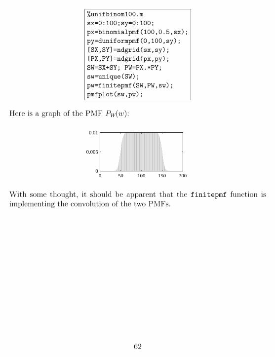
%unifbinom100.m
sx=0:100;sy=0:100;
px=binomialpmf(100,0.5,sx);
py=duniformpmf(0,100,sy);
[SX,SY]=ndgrid(sx,sy);
[PX,PY]=ndgrid(px,py);
SW=SX+SY; PW=PX.*PY;
sw=unique(SW);
pw=finitepmf(SW,PW,sw);
pmfplot(sw,pw);
Here is a graph of the PMF PW(w):
0 50 100 150 2000
0.005
0.01
With some thought, it should be apparent that the finitepmf function isimplementing the convolution of the two PMFs.
62
Quiz 10.1 SolutionAn exponential random variable with expected value 1 also has variance 1.By Theorem 10.1, Mn(X) has variance Var[Mn(X)] = 1/n. Hence, we needn = 100 samples.
Quiz 10.2 SolutionThe train interarrival times X1, X2, X3 are iid exponential (λ) random vari-ables. The arrival time of the third train is
W = X1 +X2 +X3. (1)
In Theorem 9.9, we found that the sum of three iid exponential (λ) randomvariables is an Erlang (n = 3, λ) random variable. From Appendix A, we findthat W has expected value and variance
E [W ] = 3/λ = 6, (2)
Var[W ] = 3/λ2 = 12. (3)
(a) By the Central Limit Theorem,
P [W > 20] = P
[W − 6√
12>
20− 6√12
]≈ Q
(7√3
)= 2.66× 10⁻⁵.
(b) From the Markov inequality, we know that
P [W > 20] ≤ E [W ]
20=
6
20= 0.3. (4)
(c) To use the Chebyshev inequality, we observe that E[W ] = 6 and Wnonnegative imply
P [|W − E [W ]| ≥ 14] = P [W − 6 ≥ 14] + P [W − 6 ≤ −14]︸ ︷︷ ︸=0
= P [W ≥ 20] . (5)
63
Thus
P [W ≥ 20] = P [|W − E [W ]| ≥ 14] (6)
≤ Var[W ]
142=
3
49= 0.061. (7)
(d) For the Chernoff bound, we note that the MGF of W is
φW (s) =
(λ
λ− s
)3
=1
(1− 2s)3. (8)
The Chernoff bound states that
P [W > 20] ≤ mins≥0
e−20sφX(s) = mins≥0
e−20s
(1− 2s)3. (9)
To minimize h(s) = e−20s/(1 − 2s)3, we set the derivative of h(s) tozero:
dh(s)
ds=e−20s(40s− 14)
(1− 2s)4= 0. (10)
This implies s = 7/20. Applying s = 7/20 into the Chernoff boundyields
P [W > 20] ≤ e−20s
(1− 2s)3
∣∣∣∣s= 7
20
= 0.0338.
(e) Theorem 4.11 says that for any w > 0, the CDF of the Erlang (3, λ)random variable W satisfies
FW (w) = 1−2∑
k=0
(λw)ke−λw
k!(11)
64
Equivalently, for λ = 1/2 and w = 20,
P [W > 20] = 1− FW (20)
= e−10(
1 +10
1!+
102
2!
)= 61e−10 = 0.0028. (12)
Although the Chernoff bound is weak in that it overestimates the prob-ability by a factor of 12, it is a valid bound. By contrast, the CentralLimit Theorem approximation grossly underestimates the true proba-bility.
Quiz 10.3 Solution
(a) Since X is a Bernoulli random variable with parameter p = 0.8, we canlook up in Appendix A to find that E[X] = p = 0.8 and variance
Var[X] = p(1− p) = (0.8)(0.2) = 0.16. (1)
(b) By Theorem 10.1,
Var[M100(X)] =Var[X]
100= 0.0016. (2)
(c) Theorem 10.5 uses the Chebyshev inequality to show that the samplemean satisfies
P [|Mn(X)− E [X]| ≥ c] ≤ Var[X]
nc2. (3)
Note that E[X] = PX(1) = p. To meet the specified requirement, wechoose c = 0.05 and n = 100. Since Var[X] = 0.16, we must have
0.16
100(0.05)2= α (4)
This reduces to α = 16/25 = 0.64.
65
(d) Again we use Equation (3). To meet the specified requirement, wechoose c = 0.1. Since Var[X] = 0.16, we must have
0.16
n(0.1)2≤ 0.05 (5)
The smallest value that meets the requirement is n = 320.
Quiz 10.4 Solution
Define the random variable W = (X − µX)2. Observe that V100(X) =M100(W ). By Theorem 10.10, the mean square error is
E[(M100(W )− µW )2
]=
Var[W ]
100. (1)
Observe that µX = 0 so that W = X2. Thus,
µW = E[X2]
=
∫ 1
−1x2fX (x) dx = 1/3, (2)
E[W 2]
= E[X4]
=
∫ 1
−1x4fX (x) dx = 1/5. (3)
Therefore Var[W ] = E[W 2]−µ2W = 1/5− (1/3)2 = 4/45 and the mean square
error is 4/4500 = 0.0009.
Quiz 10.5 Solution
Following the bernoullitraces.m approach, we generate m = 1000 sam-ple paths, each sample path having n = 100 Bernoulli traces. at time k,OK(k) counts the fraction of sample paths that have sample mean within onestandard error of p. The program bernoullisample.m generates graphs thenumber of traces within one standard error as a function of the time, i.e. thenumber of trials in each trace.
66
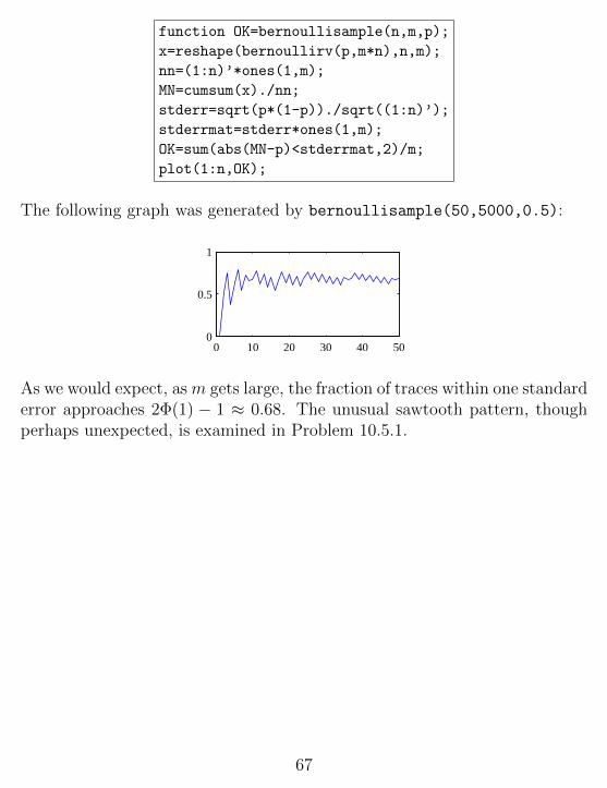
function OK=bernoullisample(n,m,p);
x=reshape(bernoullirv(p,m*n),n,m);
nn=(1:n)’*ones(1,m);
MN=cumsum(x)./nn;
stderr=sqrt(p*(1-p))./sqrt((1:n)’);
stderrmat=stderr*ones(1,m);
OK=sum(abs(MN-p)<stderrmat,2)/m;
plot(1:n,OK);
The following graph was generated by bernoullisample(50,5000,0.5):
0 10 20 30 40 500
0.5
1
As we would expect, as m gets large, the fraction of traces within one standarderror approaches 2Φ(1) − 1 ≈ 0.68. The unusual sawtooth pattern, thoughperhaps unexpected, is examined in Problem 10.5.1.
67
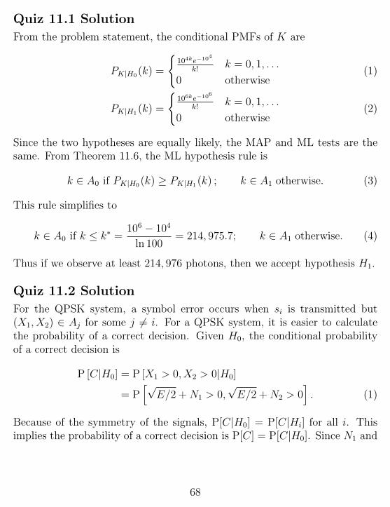
Quiz 11.1 Solution
From the problem statement, the conditional PMFs of K are
PK|H0(k) =
{104ke−104
k!k = 0, 1, . . .
0 otherwise(1)
PK|H1(k) =
{106ke−106
k!k = 0, 1, . . .
0 otherwise(2)
Since the two hypotheses are equally likely, the MAP and ML tests are thesame. From Theorem 11.6, the ML hypothesis rule is
k ∈ A0 if PK|H0(k) ≥ PK|H1(k) ; k ∈ A1 otherwise. (3)
This rule simplifies to
k ∈ A0 if k ≤ k∗ =106 − 104
ln 100= 214, 975.7; k ∈ A1 otherwise. (4)
Thus if we observe at least 214, 976 photons, then we accept hypothesis H1.
Quiz 11.2 Solution
For the QPSK system, a symbol error occurs when si is transmitted but(X1, X2) ∈ Aj for some j 6= i. For a QPSK system, it is easier to calculatethe probability of a correct decision. Given H0, the conditional probabilityof a correct decision is
P [C|H0] = P [X1 > 0, X2 > 0|H0]
= P[√
E/2 +N1 > 0,√E/2 +N2 > 0
]. (1)
Because of the symmetry of the signals, P[C|H0] = P[C|Hi] for all i. Thisimplies the probability of a correct decision is P[C] = P[C|H0]. Since N1 and
68
N2 are iid Gaussian (0, σ) random variables, we have
P [C] = P [C|H0] = P[√
E/2 +N1 > 0]
P[√
E/2 +N2 > 0]
=(
P[N1 > −
√E/2
])2=
[1− Φ
(−√E/2
σ
)]2. (2)
Since Φ(−x) = 1 − Φ(x), we have P[C] = Φ2(√E/2σ2). Equivalently, the
probability of error is
PERR = 1− P [C] = 1− Φ2
(√E
2σ2
). (3)
Quiz 11.3 Solution
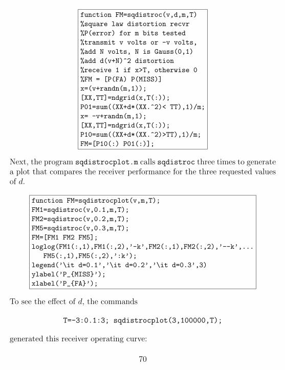
To generate the ROC, the existing program sqdistor already calculates thismiss probability PMISS = P01 and the false alarm probability PFA = P10.The modified program, sqdistroc.m is essentially the same as sqdistor
except the output is a matrix FM whose columns are the false alarm and missprobabilities. Here is the modified code:
69
function FM=sqdistroc(v,d,m,T)
%square law distortion recvr
%P(error) for m bits tested
%transmit v volts or -v volts,
%add N volts, N is Gauss(0,1)
%add d(v+N)^2 distortion
%receive 1 if x>T, otherwise 0
%FM = [P(FA) P(MISS)]
x=(v+randn(m,1));
[XX,TT]=ndgrid(x,T(:));
P01=sum((XX+d*(XX.^2)< TT),1)/m;
x= -v+randn(m,1);
[XX,TT]=ndgrid(x,T(:));
P10=sum((XX+d*(XX.^2)>TT),1)/m;
FM=[P10(:) P01(:)];
Next, the program sqdistrocplot.m calls sqdistroc three times to generatea plot that compares the receiver performance for the three requested valuesof d.
function FM=sqdistrocplot(v,m,T);
FM1=sqdistroc(v,0.1,m,T);
FM2=sqdistroc(v,0.2,m,T);
FM5=sqdistroc(v,0.3,m,T);
FM=[FM1 FM2 FM5];
loglog(FM1(:,1),FM1(:,2),’-k’,FM2(:,1),FM2(:,2),’--k’,...
FM5(:,1),FM5(:,2),’:k’);
legend(’\it d=0.1’,’\it d=0.2’,’\it d=0.3’,3)
ylabel(’P_{MISS}’);
xlabel(’P_{FA}’);
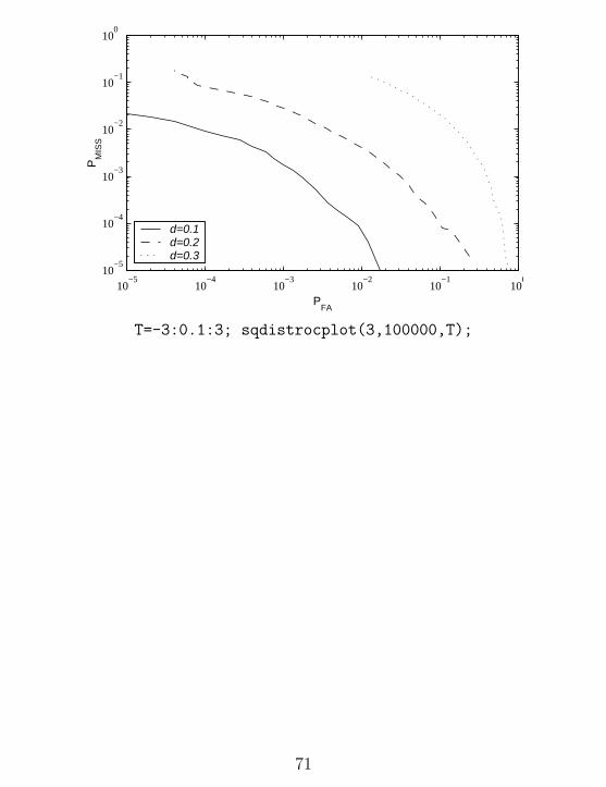
To see the effect of d, the commands
T=-3:0.1:3; sqdistrocplot(3,100000,T);
generated this receiver operating curve:
70
10−5
10−4
10−3
10−2
10−1
100
10−5
10−4
10−3
10−2
10−1
100
PM
ISS
PFA
d=0.1 d=0.2 d=0.3
T=-3:0.1:3; sqdistrocplot(3,100000,T);
71
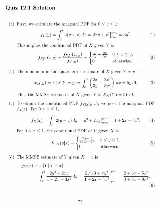
Quiz 12.1 Solution
(a) First, we calculate the marginal PDF for 0 ≤ y ≤ 1:
fY (y) =
∫ y
0
2(y + x) dx = 2xy + x2∣∣x=yx=0
= 3y2. (1)
This implies the conditional PDF of X given Y is
fX|Y (x|y) =fX,Y (x, y)
fY (y)=
{23y
+ 2x3y2
0 ≤ x ≤ y,
0 otherwise.(2)
(b) The minimum mean square error estimate of X given Y = y is
xM(y) = E [X|Y = y] =
∫ y
0
(2x
3y+
2x2
3y2
)dx = 5y/9. (3)
Thus the MMSE estimator of X given Y is XM(Y ) = 5Y/9.
(c) To obtain the conditional PDF fY |X(y|x), we need the marginal PDFfX(x). For 0 ≤ x ≤ 1,
fX (x) =
∫ 1
x
2(y + x) dy = y2 + 2xy∣∣y=1
y=x= 1 + 2x− 3x2. (4)
For 0 ≤ x ≤ 1, the conditional PDF of Y given X is
fY |X (y|x) =
{2(y+x)
1+2x−3x2 x ≤ y ≤ 1,
0 otherwise.(5)
(d) The MMSE estimate of Y given X = x is
yM(x) = E [Y |X = x]
=
∫ 1
x
2y2 + 2xy
1 + 2x− 3x2dy =
2y3/3 + xy2
1 + 2x− 3x2
∣∣∣∣y=1
y=x
=2 + 3x− 5x3
3 + 6x− 9x2.
(6)
72
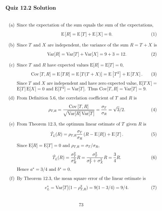
Quiz 12.2 Solution
(a) Since the expectation of the sum equals the sum of the expectations,
E [R] = E [T ] + E [X] = 0. (1)
(b) Since T and X are independent, the variance of the sum R = T +X is
Var[R] = Var[T ] + Var[X] = 9 + 3 = 12. (2)
(c) Since T and R have expected values E[R] = E[T ] = 0,
Cov [T,R] = E [TR] = E [T (T +X)] = E[T 2]
+ E [TX] . (3)
Since T and X are independent and have zero expected value, E[TX] =E[T ] E[X] = 0 and E[T 2] = Var[T ]. Thus Cov[T,R] = Var[T ] = 9.
(d) From Definition 5.6, the correlation coefficient of T and R is
ρT,R =Cov [T,R]√Var[R] Var[T ]
=σTσR
=√
3/2. (4)
(e) From Theorem 12.3, the optimum linear estimate of T given R is
TL(R) = ρT,RσTσR
(R− E [R]) + E [T ] . (5)
Since E[R] = E[T ] = 0 and ρT,R = σT/σR,
TL(R) =σ2T
σ2R
R =σ2T
σ2T + σ2
X
R =3
4R. (6)
Hence a∗ = 3/4 and b∗ = 0.
(f) By Theorem 12.3, the mean square error of the linear estimate is
e∗L = Var[T ](1− ρ2T,R) = 9(1− 3/4) = 9/4. (7)
73
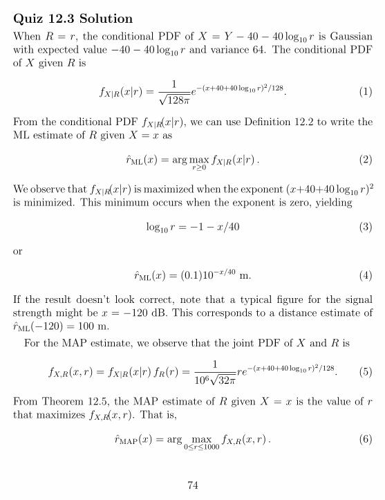
Quiz 12.3 Solution
When R = r, the conditional PDF of X = Y − 40 − 40 log10 r is Gaussianwith expected value −40 − 40 log10 r and variance 64. The conditional PDFof X given R is
fX|R(x|r) =1√
128πe−(x+40+40 log10 r)
2/128. (1)
From the conditional PDF fX|R(x|r), we can use Definition 12.2 to write theML estimate of R given X = x as
rML(x) = arg maxr≥0
fX|R(x|r) . (2)
We observe that fX|R(x|r) is maximized when the exponent (x+40+40 log10 r)2
is minimized. This minimum occurs when the exponent is zero, yielding
log10 r = −1− x/40 (3)
or
rML(x) = (0.1)10−x/40 m. (4)
If the result doesn’t look correct, note that a typical figure for the signalstrength might be x = −120 dB. This corresponds to a distance estimate ofrML(−120) = 100 m.
For the MAP estimate, we observe that the joint PDF of X and R is
fX,R(x, r) = fX|R(x|r) fR(r) =1
106√
32πre−(x+40+40 log10 r)
2/128. (5)
From Theorem 12.5, the MAP estimate of R given X = x is the value of rthat maximizes fX,R(x, r). That is,
rMAP(x) = arg max0≤r≤1000
fX,R(x, r) . (6)
74
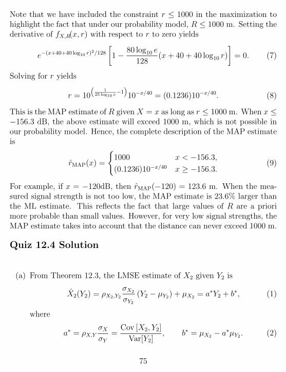
Note that we have included the constraint r ≤ 1000 in the maximization tohighlight the fact that under our probability model, R ≤ 1000 m. Setting thederivative of fX,R(x, r) with respect to r to zero yields
e−(x+40+40 log10 r)2/128
[1− 80 log10 e
128(x+ 40 + 40 log10 r)
]= 0. (7)
Solving for r yields
r = 10
(1
25 log10 e−1
)10−x/40 = (0.1236)10−x/40. (8)
This is the MAP estimate of R given X = x as long as r ≤ 1000 m. When x ≤−156.3 dB, the above estimate will exceed 1000 m, which is not possible inour probability model. Hence, the complete description of the MAP estimateis
rMAP(x) =
{1000 x < −156.3,
(0.1236)10−x/40 x ≥ −156.3.(9)
For example, if x = −120dB, then rMAP(−120) = 123.6 m. When the mea-sured signal strength is not too low, the MAP estimate is 23.6% larger thanthe ML estimate. This reflects the fact that large values of R are a priorimore probable than small values. However, for very low signal strengths, theMAP estimate takes into account that the distance can never exceed 1000 m.
Quiz 12.4 Solution
(a) From Theorem 12.3, the LMSE estimate of X2 given Y2 is
X2(Y2) = ρX2,Y2
σX2
σY2(Y2 − µY2) + µX2 = a∗Y2 + b∗, (1)
where
a∗ = ρX,YσXσY
=Cov [X2, Y2]
Var[Y2], b∗ = µX2 − a∗µY2 . (2)
75
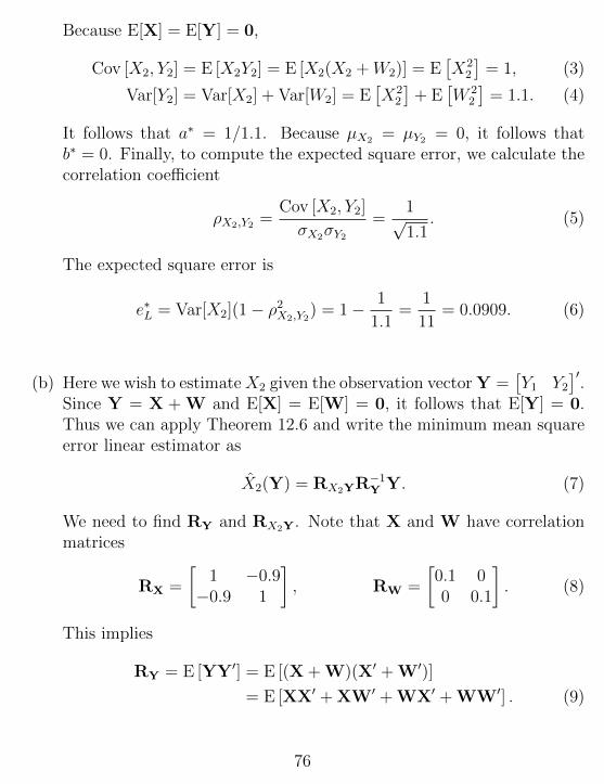
Because E[X] = E[Y] = 0,
Cov [X2, Y2] = E [X2Y2] = E [X2(X2 +W2)] = E[X2
2
]= 1, (3)
Var[Y2] = Var[X2] + Var[W2] = E[X2
2
]+ E
[W 2
2
]= 1.1. (4)
It follows that a∗ = 1/1.1. Because µX2 = µY2 = 0, it follows thatb∗ = 0. Finally, to compute the expected square error, we calculate thecorrelation coefficient
ρX2,Y2 =Cov [X2, Y2]
σX2σY2=
1√1.1
. (5)
The expected square error is
e∗L = Var[X2](1− ρ2X2,Y2) = 1− 1
1.1=
1
11= 0.0909. (6)
(b) Here we wish to estimateX2 given the observation vector Y =[Y1 Y2
]′.
Since Y = X + W and E[X] = E[W] = 0, it follows that E[Y] = 0.Thus we can apply Theorem 12.6 and write the minimum mean squareerror linear estimator as
X2(Y) = RX2YR−1Y Y. (7)
We need to find RY and RX2Y. Note that X and W have correlationmatrices
RX =
[1 −0.9−0.9 1
], RW =
[0.1 00 0.1
]. (8)
This implies
RY = E [YY′] = E [(X + W)(X′ + W′)]
= E [XX′ + XW′ + WX′ + WW′] . (9)
76
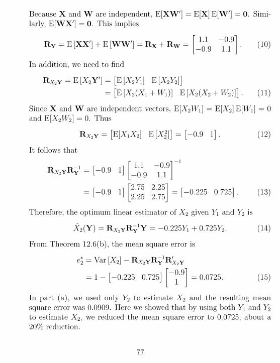
Because X and W are independent, E[XW′] = E[X] E[W′] = 0. Simi-larly, E[WX′] = 0. This implies
RY = E [XX′] + E [WW′] = RX + RW =
[1.1 −0.9−0.9 1.1
]. (10)
In addition, we need to find
RX2Y = E [X2Y′] =
[E [X2Y1] E [X2Y2]
]=[E [X2(X1 +W1)] E [X2(X2 +W2)]
]. (11)
Since X and W are independent vectors, E[X2W1] = E[X2] E[W1] = 0and E[X2W2] = 0. Thus
RX2Y =[E[X1X2] E [X2
2 ]]
=[−0.9 1
]. (12)
It follows that
RX2YR−1Y =
[−0.9 1
] [ 1.1 −0.9−0.9 1.1
]−1=[−0.9 1
] [2.75 2.252.25 2.75
]=[−0.225 0.725
]. (13)
Therefore, the optimum linear estimator of X2 given Y1 and Y2 is
X2(Y) = RX2YR−1Y Y = −0.225Y1 + 0.725Y2. (14)
From Theorem 12.6(b), the mean square error is
e∗2 = Var [X2]−RX2YR−1Y R′X2Y
= 1−[−0.225 0.725
] [−0.91
]= 0.0725. (15)
In part (a), we used only Y2 to estimate X2 and the resulting meansquare error was 0.0909. Here we showed that by using both Y1 and Y2to estimate X2, we reduced the mean square error to 0.0725, about a20% reduction.
77
Quiz 12.5 Solution
Since X and W have zero expected value, Y also has zero expected value.Thus, by Theorem 12.6,
XL(Y) = RXYR−1Y Y (1)
Since X and W are independent, E[WX] = 0 and E[XW′] = 0′. Thisimplies
RXY = E [XY′] = E [X(1′X + W′)] = 1′ E[X2]
= 1′. (2)
Note that 1′ is the row vector[1 1 · · · 1
]of twenty ones. By the same
reasoning, the correlation matrix of Y is
RY = E [YY′] = E [(1X + W)(1′X + W′)]
= 11′ E[X2]
+ 1E [XW′] + E [WX]1′ + E [WW′]
= 11′ + RW (3)
Note that 11′ is a 20× 20 matrix with every entry equal to 1. Thus,
RXYR−1Y = 1′ (11′ + RW )
−1(4)
and the optimal linear estimator is
XL(Y) = 1′ (11′ + RW)−1
Y. (5)
By Theorem 12.6(b), the mean square error is
e∗L = Var[X]−RXYR−1Y RYX = 1− 1′ (11′ + RW)
−11. (6)
Now we note that RW has i, jth entry RW(i, j) = c|i−j|−1. The questionwe must address is what value c minimizes e∗L. This problem is atypical inthat we do not usually get to choose the correlation structure of the noise.However, we will see that the answer is somewhat instructive.
We note that the optimal c is not obviously apparent from Equation (6). Inparticular, we observe that Var[Wi] = RW(i, i) = 1/c. Thus, when c is small,
78
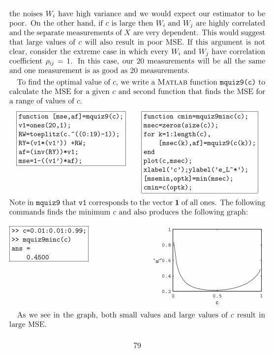
the noises Wi have high variance and we would expect our estimator to bepoor. On the other hand, if c is large then Wi and Wj are highly correlatedand the separate measurements of X are very dependent. This would suggestthat large values of c will also result in poor MSE. If this argument is notclear, consider the extreme case in which every Wi and Wj have correlationcoefficient ρij = 1. In this case, our 20 measurements will be all the sameand one measurement is as good as 20 measurements.
To find the optimal value of c, we write a Matlab function mquiz9(c) tocalculate the MSE for a given c and second function that finds the MSE fora range of values of c.
function [mse,af]=mquiz9(c);
v1=ones(20,1);
RW=toeplitz(c.^((0:19)-1));
RY=(v1*(v1’)) +RW;
af=(inv(RY))*v1;
mse=1-((v1’)*af);
function cmin=mquiz9minc(c);
msec=zeros(size(c));
for k=1:length(c),
[msec(k),af]=mquiz9(c(k));
end
plot(c,msec);
xlabel(’c’);ylabel(’e_L^*’);
[msemin,optk]=min(msec);
cmin=c(optk);
Note in mquiz9 that v1 corresponds to the vector 1 of all ones. The followingcommands finds the minimum c and also produces the following graph:
>> c=0.01:0.01:0.99;
>> mquiz9minc(c)
ans =
0.4500
0 0.5 10.2
0.4
0.6
0.8
1
c
e L*
As we see in the graph, both small values and large values of c result inlarge MSE.
79
Quiz 13.1 Solution
(a) We obtain a continuous-time, continuous-value process when we recordthe temperature as a continuous waveform over time.
(b) If at every moment in time, we round the temperature to the nearestdegree, then we obtain a continuous-time, discrete-value process.
(c) If we sample the process in part (a) every T seconds, then we obtain adiscrete-time, continuous-value process.
(d) Rounding the samples in part (c) to the nearest integer degree yields adiscrete-time, discrete-value process.
Quiz 13.2 Solution
(a) Each resistor has resistance R in ohms with uniform PDF
fR(r) =
{0.01 950 ≤ r ≤ 1050
0 otherwise(1)
The probability that a test produces a 1% resistor is
p = P [990 ≤ R ≤ 1010] =
∫ 1010
990
(0.01) dr = 0.2. (2)
(b) In t seconds, exactly t resistors are tested. Each resistor is a 1% resis-tor with probability p = 0.2, independent of any other resistor. Con-sequently, the number of 1% resistors found has the binomial (t, 0.2)PMF
PN(t)(n) =
(t
n
)(0.2)n(0.8)t−n. (3)
80
(c) First we will find the PMF of T1. This problem is easy if we view eachresistor test as an independent trial. A success occurs on a trial withprobability p = 0.2 if we find a 1% resistor. The first 1% resistor is foundat time T1 = t if we observe failures on trials 1, . . . , t− 1 followed by asuccess on trial t. Hence, just as in Example 3.8, T1 has the geometric(0.2) PMF
PT1(t) =
{(0.8)t−1(0.2) t = 1, 2, . . .
0 otherwise.(4)
From Theorem 3.5, a geometric random variable with success probabil-ity p has expected value 1/p. In this problem, E[T1] = 1/p = 5.
(d) Since p = 0.2, the probability the first 1% resistor is found in exactlyfive seconds is PT1(5) = (0.8)4(0.2) = 0.08192.
(e) Note that once we find the first 1% resistor, the number of additionaltrials needed to find the second 1% resistor once again has a geometricPMF with expected value 1/p since each independent trial is a successwith probability p. That is, T2 = T1 + T ′ where T ′ is independent andidentically distributed to T1. Thus
E [T2|T1 = 10] = E [T1|T1 = 10] + E [T ′|T1 = 10]
= 10 + E [T ′] = 10 + 5 = 15. (5)
Quiz 13.3 SolutionSince each Xi is a N(0, 1) random variable, each Xi has PDF
fXi)(x) =1√2πe−x
2/2. (1)
By Theorem 13.1, the joint PDF of X =[X1 · · ·Xn
]′is
fX(x) = fX(1),...,X(n)(x1, . . . , xn) =k∏i=1
fX (xi) =1
(2π)n/2e−(x
21+···+x2n)/2. (2)
81
Quiz 13.4 Solution
The first and second hours are nonoverlapping intervals. Since one hour equals3600 sec and the Poisson process has a rate of 10 packets/sec, the expectednumber of packets in each hour is E[Mi] = α = 36, 000. This implies M1 andM2 are independent Poisson random variables each with PMF
PMi(m) =
{αme−α
m!m = 0, 1, 2, . . .
0 otherwise(1)
Since M1 and M2 are independent, the joint PMF of M1 and M2 is
PM1,M2(m1,m2) = PM1(m1)PM2(m2) =
αm1+m2e−2α
m1!m2!m1 = 0, 1, . . . ;
m2 = 0, 1, . . . ,
0 otherwise.
(2)
Quiz 13.5 Solution
To answer whether N ′(t) is a Poisson process, we look at the interarrivaltimes. Let X1, X2, . . . denote the interarrival times of the N(t) process. Sincewe count only even-numbered arrival for N ′(t), the time until the first arrivalof the N ′(t) is Y1 = X1 +X2. Since X1 and X2 are independent exponential(λ) random variables, Y1 is an Erlang (n = 2, λ) random variable; see The-orem 9.9. Since Yi(t), the ith interarrival time of the N ′(t) process, has thesame PDF as Y1(t), we can conclude that the interarrival times of N ′(t) arenot exponential random variables. Thus N ′(t) is not a Poisson process.
Quiz 13.6 Solution
First, we note that for t > s,
X(t)−X(s) =W (t)−W (s)√
α. (1)
82
Since W (t)−W (s) is a Gaussian random variable, Theorem 4.13 states thatW (t)−W (s) is Gaussian with expected value
E [X(t)−X(s)] =E [W (t)−W (s)]√
α= 0 (2)
and variance
E[(W (t)−W (s))2
]=
E [(W (t)−W (s))2]
α=α(t− s)
α. (3)
Consider s′ ≤ s < t. Since s ≥ s′, W (t) −W (s) is independent of W (s′).This implies [W (t) −W (s)]/
√α is independent of W (s′)/
√α for all s ≥ s′.
That is, X(t) − X(s) is independent of X(s′) for all s ≥ s′. Thus X(t) is aBrownian motion process with variance Var[X(t)] = t.
Quiz 13.7 Solution
First we find the expected value
µY (t) = µX(t) + µN(t) = µX(t). (1)
To find the autocorrelation, we observe that since X(t) and N(t) are indepen-dent and sinceN(t) has zero expected value, E[X(t)N(t′)] = E[X(t)] E[N(t′)] =0. Since RY (t, τ) = E[Y (t)Y (t+ τ)], we have
RY (t, τ) = E [(X(t) +N(t)) (X(t+ τ) +N(t+ τ))]
= E [X(t)X(t+ τ)] + E [X(t)N(t+ τ)]
+ E [X(t+ τ)N(t)] + E [N(t)N(t+ τ)]
= RX(t, τ) +RN(t, τ). (2)
Quiz 13.8 Solution
From Definition 13.14, X1, X2, . . . is a stationary random sequence if for allsets of time instants n1, . . . , nm and time offset k,
fXn1 ,...,Xnm (x1, . . . , xm) = fXn1+k,...,Xnm+k(x1, . . . , xm) . (1)
83
Since the random sequence is iid,
fXn1 ,...,Xnm (x1, . . . , xm) = fX (x1) fX (x2) · · · fX (xm) . (2)
Similarly, for time instants n1 + k, . . . , nm + k,
fXn1+k,...,Xnm+k(x1, . . . , xm) = fX (x1) fX (x2) · · · fX (xm) . (3)
We can conclude that the iid random sequence is stationary.
Quiz 13.9 SolutionWe must check whether each function R(τ) meets the conditions of Theo-rem 13.12:
R(τ) ≥ 0, R(τ) = R(−τ), |R(τ)| ≤ R(0). (1)
(a) R1(τ) = e−|τ | meets all three conditions and thus is valid.
(b) R2(τ) = e−τ2
also is valid.
(c) R3(τ) = e−τ cos τ is not valid because
R3(−2π) = e2π cos 2π = e2π > 1 = R3(0) (2)
(d) R4(τ) = e−τ2
sin τ also cannot be an autocorrelation function because
R4(π/2) = e−π/2 sinπ/2 = e−π/2 > 0 = R4(0) (3)
Quiz 13.10 Solution
(a) The autocorrelation of Y (t) is
RY (t, τ) = E [Y (t)Y (t+ τ)]
= E [X(−t)X(−t− τ)]
= RX(−t− (−t− τ)) = RX(τ). (1)
Since E[Y (t)] = E[X(−t)] = µX , we can conclude that Y (t) is a widesense stationary process. In fact, we see that by viewing a processbackwards in time, we see the same second order statistics.
84
(b) Since X(t) and Y (t) are both wide sense stationary processes, we cancheck whether they are jointly wide sense stationary by seeing ifRXY (t, τ)is just a function of τ . In this case,
RXY (t, τ) = E [X(t)Y (t+ τ)]
= E [X(t)X(−t− τ)]
= RX(t− (−t− τ)) = RX(2t+ τ). (2)
Since RXY (t, τ) depends on both t and τ , we conclude that X(t) andY (t) are not jointly wide sense stationary. To see why this is, supposeRX(τ) = e−|τ | so that samples of X(t) far apart in time have almostno correlation. In this case, as t gets larger, Y (t) = X(−t) and X(t)become less correlated.
Quiz 13.11 SolutionFrom the problem statement,
E [X(t)] = E [X(t+ 1)] = 0, (1)
E [X(t)X(t+ 1)] = 1/2, (2)
Var[X(t)] = Var[X(t+ 1)] = 1. (3)
The Gaussian random vector X =[X(t) X(t+ 1)
]′has covariance matrix
and corresponding inverse
CX =
[1 1/2
1/2 1
], C−1X =
4
3
[1 −1/2−1/2 1
]. (4)
Since
x′C−1X x =[x0 x1
]′ 43
[1 −1/2−1/2 1
] [x0x1
]=
4
3
(x20 − x0x+x21
), (5)
the joint PDF of X(t) and X(t+ 1) is the Gaussian vector PDF
fX(t),X(t+1)(x0, x1) =1
(2π)n/2[det (CX)]1/2exp
(−1
2x′C−1X x
)(6)
=1√3π2
e−23(x20−x0x1+x21). (7)
85
Quiz 13.12 Solution
The simple structure of the switch simulation of Example 13.22 admits adeceptively simple solution in terms of the vector of arrivals A and the vectorof departures D. With the introduction of call blocking. we cannot generatethese vectors all at once. In particular, when an arrival occurs at time t, weneed to know that M(t), the number of ongoing calls, satisfies M(t) < c =120. Otherwise, when M(t) = c, we must block the call. Call blocking canbe implemented by setting the service time of the call to zero so that the calldeparts as soon as it arrives.
The blocking switch is an example of a discrete event system. The systemevolves via a sequence of discrete events, namely arrivals and departures, atdiscrete time instances. A simulation of the system moves from one timeinstant to the next by maintaining a chronological schedule of future events(arrivals and departures) to be executed. The program simply executes theevent at the head of the schedule. The logic of such a simulation is
1. Start at time t = 0 with an empty system. Schedule the first arrival tooccur at S1, an exponential (λ) random variable.
2. Examine the head-of-schedule event.
• When the head-of-schedule event is the kth arrival is at time t,check the state M(t).
– If M(t) < c, admit the arrival, increase the system state n by1, and schedule a departure to occur at time t+ Sn, where Skis an exponential (λ) random variable.
– If M(t) = c, block the arrival, do not schedule a departureevent.
• If the head of schedule event is a departure, reduce the systemstate n by 1.
3. Delete the head-of-schedule event and go to step 2.
86

After the head-of-schedule event is completed and any new events (departuresin this system) are scheduled, we know the system state cannot change untilthe next scheduled event. Thus we know that M(t) will stay the same untilthen. In our simulation, we use the vector t as the set of time instancesat which we inspect the system state. Thus for all times t(i) between thecurrent head-of-schedule event and the next, we set m(i) to the current switchstate. Here is the complete program:
87
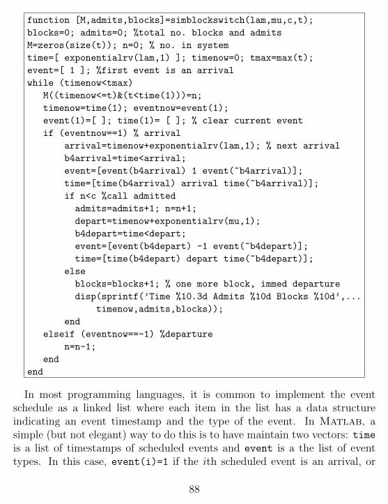
function [M,admits,blocks]=simblockswitch(lam,mu,c,t);
blocks=0; admits=0; %total no. blocks and admits
M=zeros(size(t)); n=0; % no. in system
time=[ exponentialrv(lam,1) ]; timenow=0; tmax=max(t);
event=[ 1 ]; %first event is an arrival
while (timenow<tmax)
M((timenow<=t)&(t<time(1)))=n;
timenow=time(1); eventnow=event(1);
event(1)=[ ]; time(1)= [ ]; % clear current event
if (eventnow==1) % arrival
arrival=timenow+exponentialrv(lam,1); % next arrival
b4arrival=time<arrival;
event=[event(b4arrival) 1 event(~b4arrival)];
time=[time(b4arrival) arrival time(~b4arrival)];
if n<c %call admitted
admits=admits+1; n=n+1;
depart=timenow+exponentialrv(mu,1);
b4depart=time<depart;
event=[event(b4depart) -1 event(~b4depart)];
time=[time(b4depart) depart time(~b4depart)];
else
blocks=blocks+1; % one more block, immed departure
disp(sprintf(’Time %10.3d Admits %10d Blocks %10d’,...
timenow,admits,blocks));
end
elseif (eventnow==-1) %departure
n=n-1;
end
end
In most programming languages, it is common to implement the eventschedule as a linked list where each item in the list has a data structureindicating an event timestamp and the type of the event. In Matlab, asimple (but not elegant) way to do this is to have maintain two vectors: timeis a list of timestamps of scheduled events and event is a the list of eventtypes. In this case, event(i)=1 if the ith scheduled event is an arrival, or
88
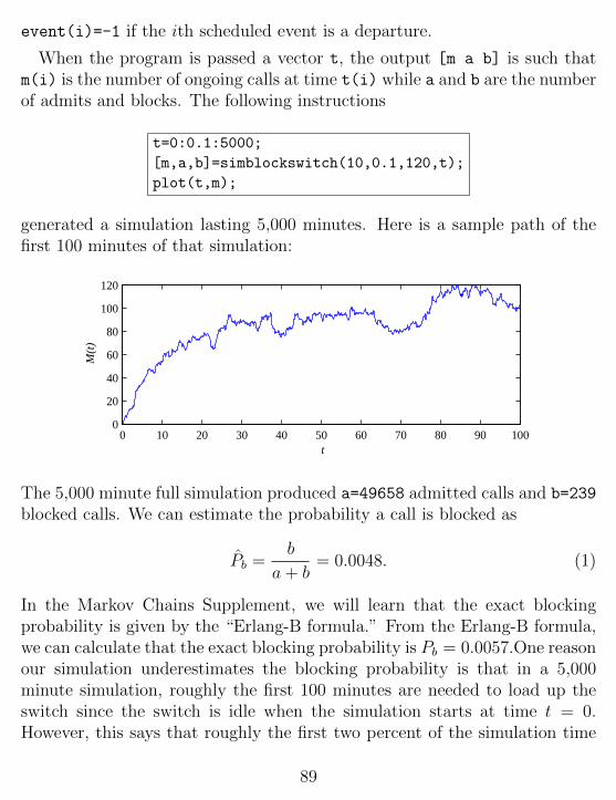
event(i)=-1 if the ith scheduled event is a departure.
When the program is passed a vector t, the output [m a b] is such thatm(i) is the number of ongoing calls at time t(i) while a and b are the numberof admits and blocks. The following instructions
t=0:0.1:5000;
[m,a,b]=simblockswitch(10,0.1,120,t);
plot(t,m);
generated a simulation lasting 5,000 minutes. Here is a sample path of thefirst 100 minutes of that simulation:
0 10 20 30 40 50 60 70 80 90 1000
20
40
60
80
100
120
t
M(t
)
The 5,000 minute full simulation produced a=49658 admitted calls and b=239
blocked calls. We can estimate the probability a call is blocked as
Pb =b
a+ b= 0.0048. (1)
In the Markov Chains Supplement, we will learn that the exact blockingprobability is given by the “Erlang-B formula.” From the Erlang-B formula,we can calculate that the exact blocking probability is Pb = 0.0057.One reasonour simulation underestimates the blocking probability is that in a 5,000minute simulation, roughly the first 100 minutes are needed to load up theswitch since the switch is idle when the simulation starts at time t = 0.However, this says that roughly the first two percent of the simulation time
89

was unusual. Thus this would account for only part of the disparity. The restof the gap between 0.0048 and 0.0057 is that a simulation that includes only239 blocks is not all that likely to give a very accurate result for the blockingprobability.
90