2 Probability and Stochastic Processes - University of …courses.ece.ubc.ca/564/chapter2.pdf9 2...

9

2 Probability and Stochastic Processes

Motivation:

� Very important mathematical tools for the design and analysis of

communication systems

� Examples:

– The transmitted symbols are unknown at the receiver and are

modeled as random variables.

– Impairments such as noise and interference are also unknown

at the receiver and are modeled as stochastic processes.

2.1 Probability

2.1.1 Basic Concepts

Given: Sample space S containing all possible outcomes of an exper-

iment

Definitions:

� Events A and B are subsets of S, i.e., A ⊆ S, B ⊆ S

� The complement of A is denoted by A and contains all elements

of S not included in A

� Union of two events: D = A∪B consists of all elements of A and

B

⇒ A ∪ A = S

Schober: Signal Detection and Estimation

10

� Intersection of two elements: E = A ∩BMutually exclusive events have as intersection the null element ◦/e.g. A ∩ A = ◦/.

� Associated with each event A is its probability P (A)

Axioms of Probability

1. P (S) = 1 (certain event)

2. 0 ≤ P (A) ≤ 1

3. If A ∩ B = ◦/ then P (A ∪B) = P (A) + P (B)

The entire theory of probability is based on these three axioms.

E.g. it can be proved that

� P (A) = 1 − P (A)

� A ∩B 6= ◦/ then P (A ∪ B) = P (A) + P (B) − P (A ∩ B)

Example:

Fair die

– S = {1, 2, 3, 4, 5, 6}– A = {1, 2, 5}, B = {3, 4, 5}– A = {3, 4, 6}– D = A ∪B = {1, 2, 3, 4, 5}– E = A ∩B = {5}– P (1) = P (2) = . . . = P (6) = 1

6


11

– P (A) = P (1) + P (2) + P (5) = 12, P (B) = 1

2

– P (D) = P (A) + P (B) − P (A ∩ B) = 12

+ 12− 1

6= 5

6

Joint Events and Joint Probabilities

� Now we consider two experiments with outcomes

Ai, i = 1, 2, . . . n

and

Bj, j = 1, 2, . . .m

� We carry out both experiments and assign the outcome (Ai, Bj)

the probability P (Ai, Bj) with

0 ≤ P (Ai, Bj) ≤ 1

� If the outcomes Bj, j = 1, 2, . . . , m are mutually exclusive we

getm

∑

j=1

P (Ai, Bj) = P (Ai)

A similar relation holds if the outcomes of Ai, i = 1, 2, . . . n are

mutually exclusive.

� If all outcomes of both experiments are mutually exclusive, then

n∑

i=1

m∑

j=1

P (Ai, Bj) = 1


12

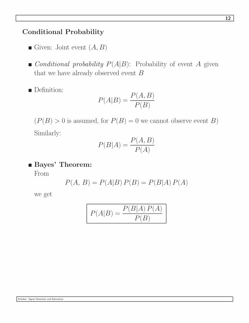
Conditional Probability

� Given: Joint event (A,B)

� Conditional probability P (A|B): Probability of event A given

that we have already observed event B

� Definition:

P (A|B) =P (A,B)

P (B)

(P (B) > 0 is assumed, for P (B) = 0 we cannot observe event B)

Similarly:

P (B|A) =P (A,B)

P (A)

� Bayes’ Theorem:

From

P (A, B) = P (A|B)P (B) = P (B|A)P (A)

we get

P (A|B) =P (B|A)P (A)

P (B)


13

Statistical Independence

If observing B does not change the probability of observing A, i.e.,

P (A|B) = P (A),

then A and B are statistically independent.

In this case:

P (A,B) = P (A|B)P (B)

= P (A)P (B)

Thus, two events A and B are statistically independent if and only if

P (A,B) = P (A)P (B)


14

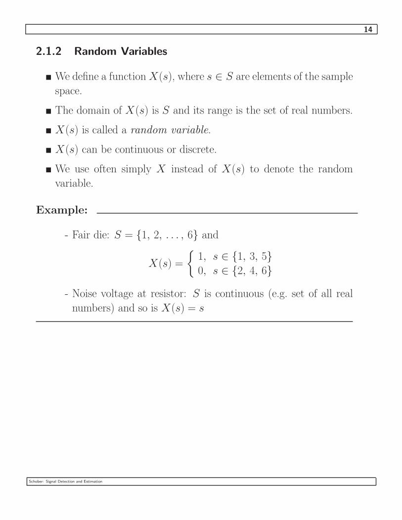
2.1.2 Random Variables

� We define a functionX(s), where s ∈ S are elements of the sample

space.

� The domain of X(s) is S and its range is the set of real numbers.

� X(s) is called a random variable.

� X(s) can be continuous or discrete.

� We use often simply X instead of X(s) to denote the random

variable.

Example:

- Fair die: S = {1, 2, . . . , 6} and

X(s) =

{

1, s ∈ {1, 3, 5}0, s ∈ {2, 4, 6}

- Noise voltage at resistor: S is continuous (e.g. set of all real

numbers) and so is X(s) = s


15

Cumulative Distribution Function (CDF)

� Definition: F (x) = P (X ≤ x)

The CDF F (x) denotes the probability that the random variable

(RV) X is smaller than or equal to x.

� Properties:

0 ≤ F (x) ≤ 1

limx→−∞

F (x) = 0

limx→∞

F (x) = 1

d

dxF (x) ≥ 0

Example:

1. Fair die X = X(s) = s

1

21 3 4 5 6

1/6

x

F (x)

Note: X is a discrete random variable.


16

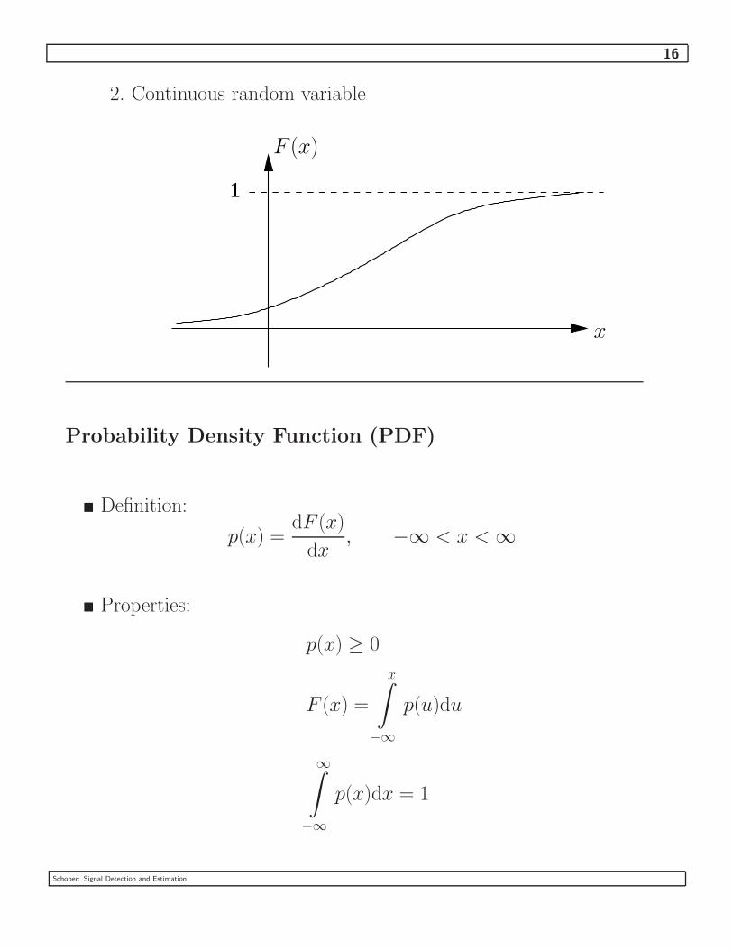
2. Continuous random variable

1

x

F (x)

Probability Density Function (PDF)

� Definition:

p(x) =dF (x)

dx, −∞ < x <∞

� Properties:

p(x) ≥ 0

F (x) =

x∫

−∞

p(u)du

∞∫

−∞

p(x)dx = 1


17

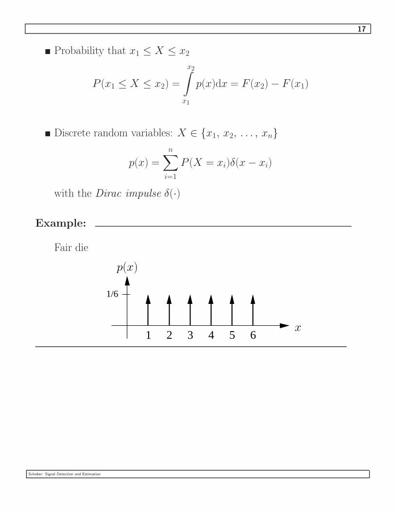
� Probability that x1 ≤ X ≤ x2

P (x1 ≤ X ≤ x2) =

x2∫

x1

p(x)dx = F (x2) − F (x1)

� Discrete random variables: X ∈ {x1, x2, . . . , xn}

p(x) =

n∑

i=1

P (X = xi)δ(x− xi)

with the Dirac impulse δ(·)

Example:

Fair die

1 32 4 5 6

1/6

x

p(x)


18

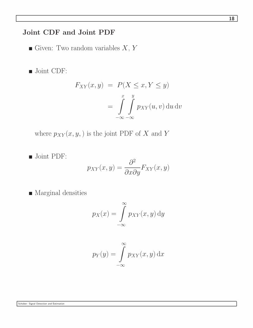
Joint CDF and Joint PDF

� Given: Two random variables X , Y

� Joint CDF:

FXY (x, y) = P (X ≤ x, Y ≤ y)

=

x∫

−∞

y∫

−∞

pXY (u, v) du dv

where pXY (x, y, ) is the joint PDF of X and Y

� Joint PDF:

pXY (x, y) =∂2

∂x∂yFXY (x, y)

� Marginal densities

pX(x) =

∞∫

−∞

pXY (x, y) dy

pY (y) =

∞∫

−∞

pXY (x, y) dx


19

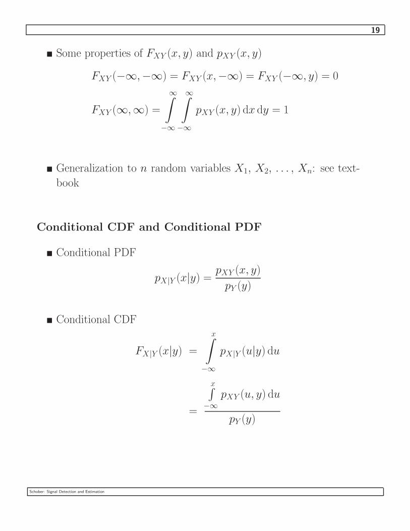
� Some properties of FXY (x, y) and pXY (x, y)

FXY (−∞,−∞) = FXY (x,−∞) = FXY (−∞, y) = 0

FXY (∞,∞) =

∞∫

−∞

∞∫

−∞

pXY (x, y) dx dy = 1

� Generalization to n random variables X1, X2, . . . , Xn: see text-

book

Conditional CDF and Conditional PDF

� Conditional PDF

pX|Y (x|y) =pXY (x, y)

pY (y)

� Conditional CDF

FX|Y (x|y) =

x∫

−∞

pX|Y (u|y) du

=

x∫

−∞pXY (u, y) du

pY (y)


20

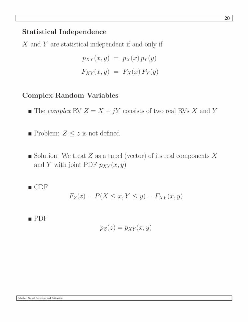
Statistical Independence

X and Y are statistical independent if and only if

pXY (x, y) = pX(x) pY (y)

FXY (x, y) = FX(x)FY (y)

Complex Random Variables

� The complex RV Z = X + jY consists of two real RVs X and Y

� Problem: Z ≤ z is not defined

� Solution: We treat Z as a tupel (vector) of its real components X

and Y with joint PDF pXY (x, y)

� CDF

FZ(z) = P (X ≤ x, Y ≤ y) = FXY (x, y)

� PDF

pZ(z) = pXY (x, y)


21

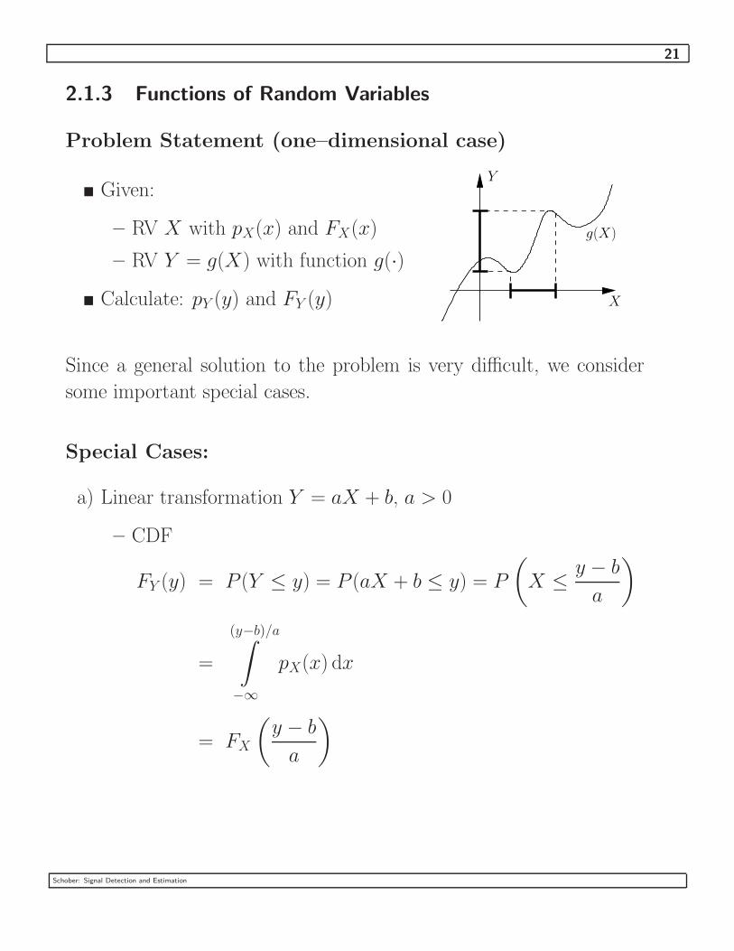
2.1.3 Functions of Random Variables

Problem Statement (one–dimensional case)

� Given:

– RV X with pX(x) and FX(x)

– RV Y = g(X) with function g(·)� Calculate: pY (y) and FY (y)

Y

X

g(X)

Since a general solution to the problem is very difficult, we consider

some important special cases.

Special Cases:

a) Linear transformation Y = aX + b, a > 0

– CDF

FY (y) = P (Y ≤ y) = P (aX + b ≤ y) = P

(

X ≤ y − b

a

)

=

(y−b)/a∫

−∞

pX(x) dx

= FX

(

y − b

a

)


22

– PDF

pY (y) =∂

∂yFY (y) =

∂

∂y

∂x

∂xFX(x)

∣

∣

∣

∣

∣

x=(y−b)/a

=∂x

∂y

∣

∣

∣

∣

∣

x=(y−b)/a

∂

∂xFX(x)

∣

∣

∣

∣

∣

x=(y−b)/a

=1

apX

(

y − b

a

)

b) g(x) = y has real roots x1, x2, . . . , xn

– PDF

pY (y) =n

∑

i=1

pX(xi)

|g′(xi)|

with g′(xi) = ddxg(x)

∣

∣

∣

∣

∣

x=xi

– CDF: Can be obtained from PDF by integration.

Example:

Y = aX2 + b, a > 0


23

Roots:

ax2 + b = y ⇒ x1/2 = ±√

y − b

a

g′(xi):d

dxg(x) = 2ax

PDF:

pY (y) =

pX

(

√

y−ba

)

2a√

y−ba

+

pX

(

−√

y−ba

)

2a√

y−ba

c) A simple multi–dimensional case

– Given:

∗ RVs Xi, 1 ≤ i ≤ n with joint PDF pX(x1, x2, . . . , xn)

∗ Transformation: Yi = gi(x1, x2, . . . , xn), 1 ≤ i ≤ n

– Problem: Calculate pY (y1, y2, . . . , yn)

– Simplifying assumptions for gi(x1, x2, . . . , xn), 1 ≤ i ≤ n

∗ gi(x1, x2, . . . , xn), 1 ≤ i ≤ n, have continuous partial

derivatives


24

∗ gi(x1, x2, . . . , xn), 1 ≤ i ≤ n, are invertible, i.e.,

Xi = g−1i (Y1, Y2, . . . , Yn), 1 ≤ i ≤ n

– PDF:

pY (y1, y2, . . . , yn) = pX(x1 = g−11 , . . . , xn = g−1

n ) · |J |

with

∗ g−1i = g−1

i (y1, y2, . . . , yn)

∗ Jacobian of transformation

J =

∂(g−11 )

∂y1· · · ∂(g−1

n )∂y1... ...

∂(g−11 )

∂yn· · · ∂(g−1

n )∂yn

∗ |J |: Determinant of matrix J

d) Sum of two RVs X1 and X2

Y = X1 +X2

– Given: pX1X2(x1, x2)

– Problem: Find pY (y)


25

– Solution:

From x1 = y − x2 we obtain the joint PDF of Y and X2

⇒ pY X2(y, x2) = pX1X2

(x1, x2)

∣

∣

∣

∣

∣

x1=y−x2

= pX1X2(y − x2, x2)

pY (y) is a marginal density of pY X2(y, x2):

⇒ pY (y) =

∞∫

−∞

pYX2(y, x2) dx2 =

∞∫

−∞

pX1X2(y − x2, x2) dx2

=

∞∫

−∞

pX1X2(x1, y − x1) dx1

– Important special case: X1 and X2 are statistically indepen-

dent

pX1X2(x1, x2) = pX1

(x1) pX2(x2)

pY (y) =

∞∫

−∞

pX1(x1)pX2

(y − x1) dx1 = pX1(x1) ∗ pX2

(x2)

The PDF of Y is simply the convolution of the PDFs of X1

and X2.


26

2.1.4 Statistical Averages of RVs

� Important for characterization of random variables.

General Case

� Given:

– RV Y = g(X) with random vector X = (X1, X2, . . . , Xn)

– (Joint) PDF pX(x) of X

� Expected value of Y :

E{Y } = E{g(X)} =

∞∫

−∞

· · ·∞

∫

−∞

g(x) pX(x) dx1 . . . dxn

E{·} denotes statistical averaging.

Special Cases (one–dimensional): X = X1 = X

� Mean: g(X) = X

mX = E{X} =

∞∫

−∞

x pX(x) dx

� nth moment: g(X) = Xn

E{Xn} =

∞∫

−∞

xn pX(x) dx


27

� nth central moment: g(X) = (X −mX)n

E{(X −mX)n} =

∞∫

−∞

(x−mX)n pX(x) dx

� Variance: 2nd central moment

σ2X =

∞∫

−∞

(x−mX)2 pX(x) dx

=

∞∫

−∞

x2 pX(x) dx +

∞∫

−∞

m2X pX(x) dx− 2

∞∫

−∞

mX x pX(x) dx

=

∞∫

−∞

x2 pX(x) dx−m2X

= E{X2} − (E{X})2

Complex case: σ2X = E{|X|2} − |E{X}|2

� Characteristic function: g(X) = ejvX

ψ(jv) = E{ejvX} =

∞∫

−∞

ejvx pX(x) dx


28

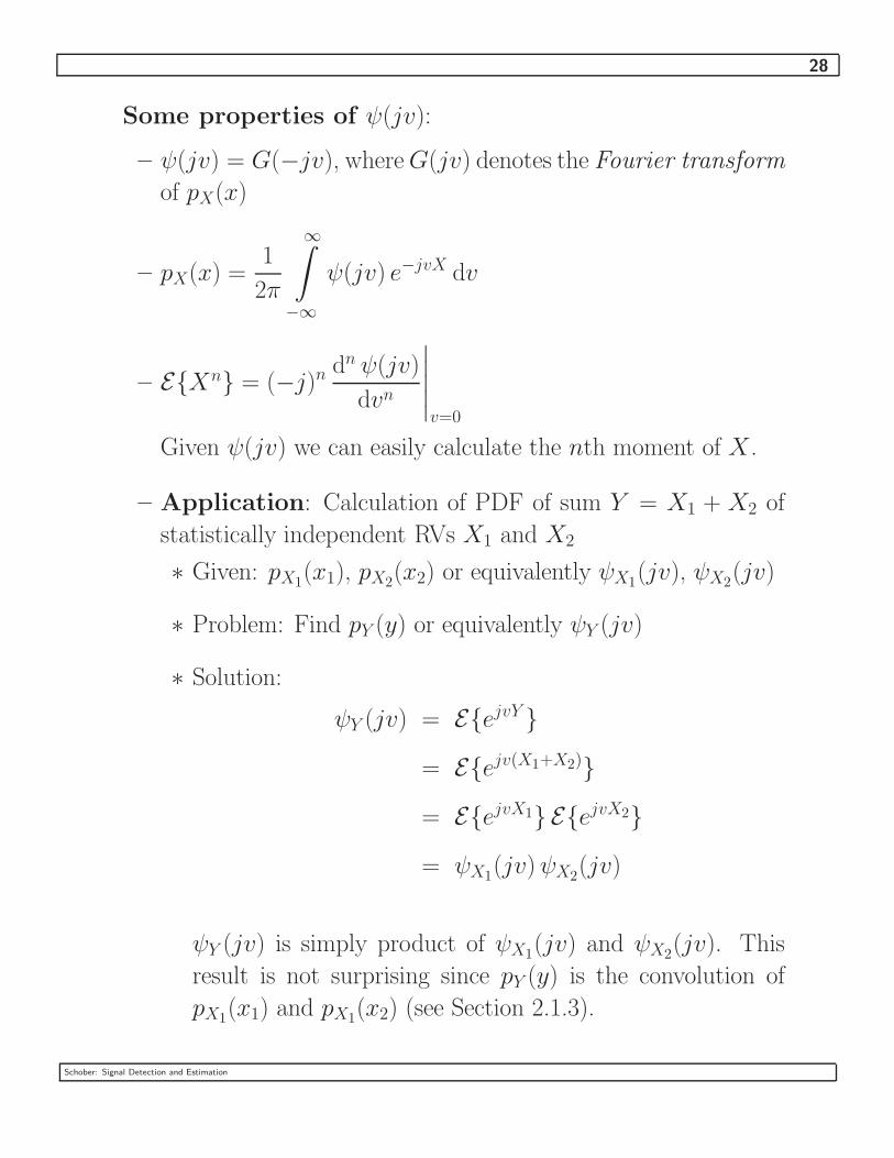
Some properties of ψ(jv):

– ψ(jv) = G(−jv), whereG(jv) denotes the Fourier transform

of pX(x)

– pX(x) =1

2π

∞∫

−∞

ψ(jv) e−jvX dv

– E{Xn} = (−j)n dn ψ(jv)

dvn

∣

∣

∣

∣

∣

v=0

Given ψ(jv) we can easily calculate the nth moment of X .

– Application: Calculation of PDF of sum Y = X1 + X2 of

statistically independent RVs X1 and X2

∗ Given: pX1(x1), pX2

(x2) or equivalently ψX1(jv), ψX2

(jv)

∗ Problem: Find pY (y) or equivalently ψY (jv)

∗ Solution:

ψY (jv) = E{ejvY }

= E{ejv(X1+X2)}

= E{ejvX1} E{ejvX2}

= ψX1(jv)ψX2

(jv)

ψY (jv) is simply product of ψX1(jv) and ψX2

(jv). This

result is not surprising since pY (y) is the convolution of

pX1(x1) and pX1

(x2) (see Section 2.1.3).


29

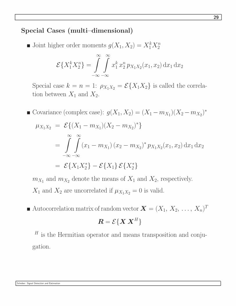
Special Cases (multi–dimensional)

� Joint higher order moments g(X1, X2) = Xk1X

n2

E{Xk1X

n2 } =

∞∫

−∞

∞∫

−∞

xk1 xn2 pX1X2

(x1, x2) dx1 dx2

Special case k = n = 1: ρX1X2= E{X1X2} is called the correla-

tion between X1 and X2.

� Covariance (complex case): g(X1, X2) = (X1−mX1)(X2−mX2

)∗

µX1X2= E{(X1 −mX1

)(X2 −mX2)∗}

=

∞∫

−∞

∞∫

−∞

(x1 −mX1) (x2 −mX2

)∗ pX1X2(x1, x2) dx1 dx2

= E{X1X∗2} − E{X1} E{X∗

2}

mX1and mX2

denote the means of X1 and X2, respectively.

X1 and X2 are uncorrelated if µX1X2= 0 is valid.

� Autocorrelation matrix of random vector X = (X1, X2, . . . , Xn)T

R = E{X XH}H is the Hermitian operator and means transposition and conju-

gation.


30

� Covariance matrix

M = E{(X − mX) (X − mX)H}

= R − mXmHX

with mean vector mX = E{X}

� Characteristic function (two–dimensional case): g(X1, X2) = ej(v1X1+v2X2)

ψ(jv1, jv2) =

∞∫

−∞

∞∫

−∞

ej(v1x1+v2x2) pX1X2(x1, x2) dx1 dx2

ψ(jv1, jv2) can be applied to calculate the joint (higher order)

moments of X1 and X2.

E.g. E{X1X2} = −∂2ψ(jv1, jv2)

∂v1∂v2

∣

∣

∣

∣

∣

v1=v2=0


31

2.1.5 Gaussian Distribution

The Gaussian distribution is the most important probability distribu-

tion in practice:

� Many physical phenomena can be described by a Gaussian distri-

bution.

� Often we also assume that a certain RV has a Gaussian distribu-

tion in order to render a problem mathematical tractable.

Real One–dimensional Case

� PDF of Gaussian RV X with mean mX and variance σ2

p(x) =1√2πσ

e−(x−mX )2/(2σ2)

Note: The Gaussian PDF is fully characterized by its first and

second order moments!

� CDF

F (x) =

x∫

−∞

p(u) du =1√2πσ

x∫

−∞

e−(u−mX)2/(2σ2) du

=1

2

2√π

x−mX√2σ

∫

−∞

e−t2

dt =1

2+

1

2erf

(

x−mX√2σ

)


32

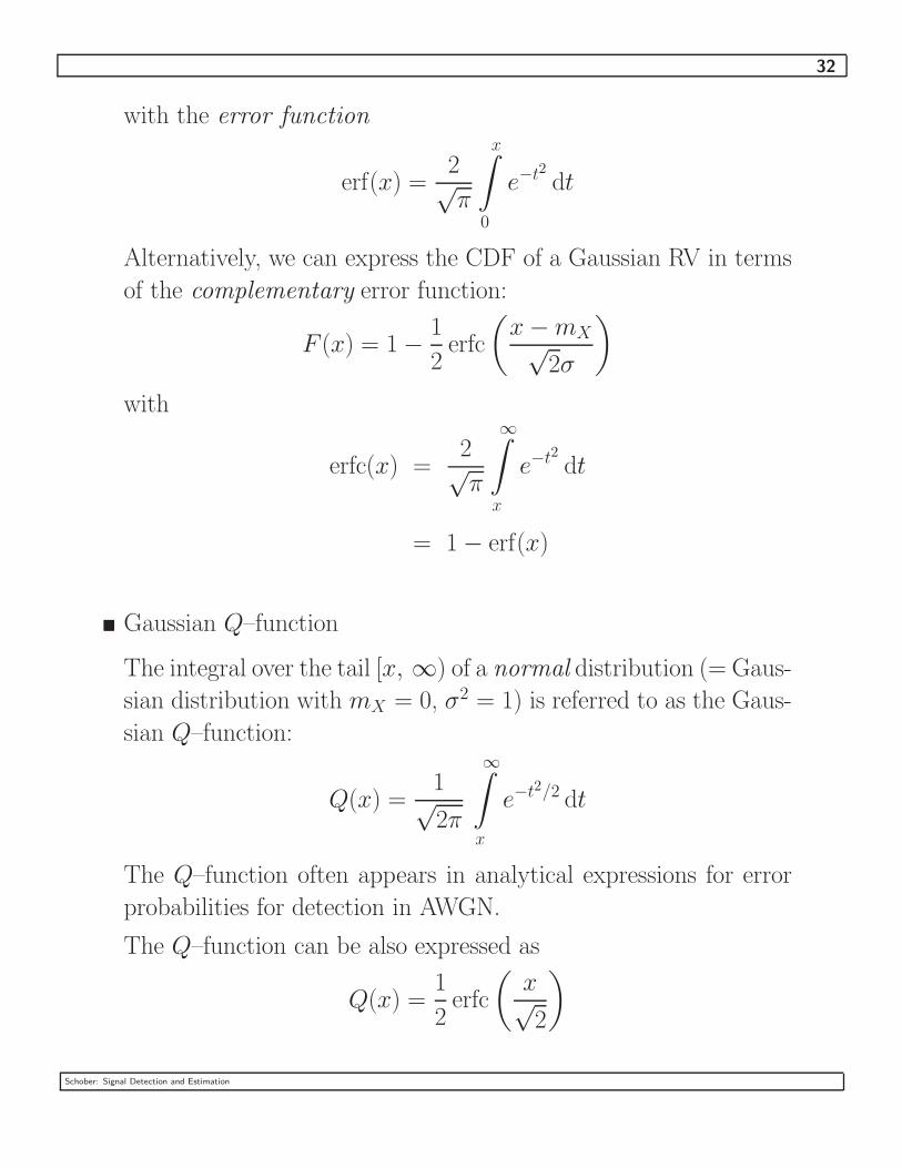
with the error function

erf(x) =2√π

x∫

0

e−t2

dt

Alternatively, we can express the CDF of a Gaussian RV in terms

of the complementary error function:

F (x) = 1 − 1

2erfc

(

x−mX√2σ

)

with

erfc(x) =2√π

∞∫

x

e−t2

dt

= 1 − erf(x)

� Gaussian Q–function

The integral over the tail [x, ∞) of a normal distribution (= Gaus-

sian distribution with mX = 0, σ2 = 1) is referred to as the Gaus-

sian Q–function:

Q(x) =1√2π

∞∫

x

e−t2/2 dt

The Q–function often appears in analytical expressions for error

probabilities for detection in AWGN.

The Q–function can be also expressed as

Q(x) =1

2erfc

(

x√2

)


33

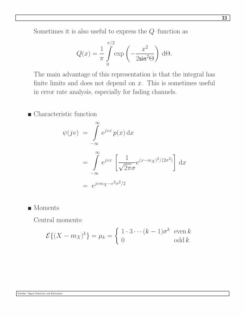
Sometimes it is also useful to express the Q–function as

Q(x) =1

π

π/2∫

0

exp

(

− x2

2sin2Θ

)

dΘ.

The main advantage of this representation is that the integral has

finite limits and does not depend on x. This is sometimes useful

in error rate analysis, especially for fading channels.

� Characteristic function

ψ(jv) =

∞∫

−∞

ejvx p(x) dx

=

∞∫

−∞

ejvx[

1√2πσ

e(x−mX)2/(2σ2)

]

dx

= ejvmX−v2σ2/2

� Moments

Central moments:

E{(X −mX)k} = µk =

{

1 · 3 · · · (k − 1)σk even k

0 odd k


34

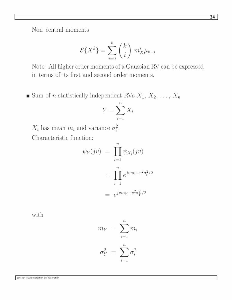
Non–central moments

E{Xk} =k

∑

i=0

(

k

i

)

miXµk−i

Note: All higher order moments of a Gaussian RV can be expressed

in terms of its first and second order moments.

� Sum of n statistically independent RVs X1, X2, . . . , Xn

Y =n

∑

i=1

Xi

Xi has mean mi and variance σ2i .

Characteristic function:

ψY (jv) =n

∏

i=1

ψXi(jv)

=n

∏

i=1

ejvmi−v2σ2i /2

= ejvmY −v2σ2Y/2

with

mY =

n∑

i=1

mi

σ2Y =

n∑

i=1

σ2i


35

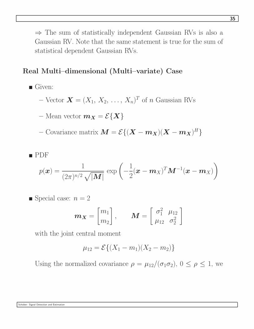
⇒ The sum of statistically independent Gaussian RVs is also a

Gaussian RV. Note that the same statement is true for the sum of

statistical dependent Gaussian RVs.

Real Multi–dimensional (Multi–variate) Case

� Given:

– Vector X = (X1, X2, . . . , Xn)T of n Gaussian RVs

– Mean vector mX = E{X}

– Covariance matrix M = E{(X − mX)(X − mX)H}

� PDF

p(x) =1

(2π)n/2√

|M |exp

(

−1

2(x − mX)TM−1(x − mX)

)

� Special case: n = 2

mX =

[

m1

m2

]

, M =

[

σ21 µ12

µ12 σ22

]

with the joint central moment

µ12 = E{(X1 −m1)(X2 −m2)}

Using the normalized covariance ρ = µ12/(σ1σ2), 0 ≤ ρ ≤ 1, we


36

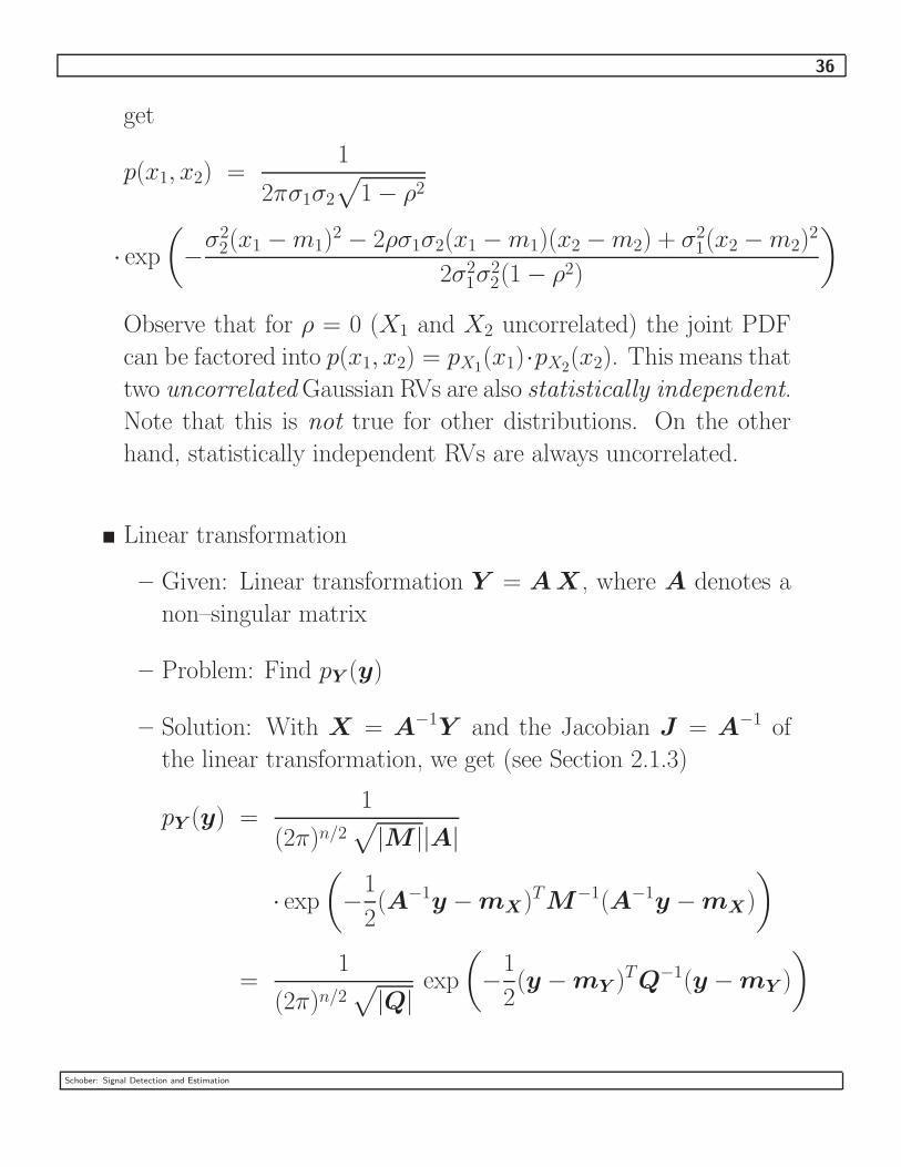
get

p(x1, x2) =1

2πσ1σ2

√

1 − ρ2

· exp

(

−σ22(x1 −m1)

2 − 2ρσ1σ2(x1 −m1)(x2 −m2) + σ21(x2 −m2)

2

2σ21σ

22(1 − ρ2)

)

Observe that for ρ = 0 (X1 and X2 uncorrelated) the joint PDF

can be factored into p(x1, x2) = pX1(x1)·pX2

(x2). This means that

two uncorrelated Gaussian RVs are also statistically independent.

Note that this is not true for other distributions. On the other

hand, statistically independent RVs are always uncorrelated.

� Linear transformation

– Given: Linear transformation Y = A X , where A denotes a

non–singular matrix

– Problem: Find pY (y)

– Solution: With X = A−1Y and the Jacobian J = A−1 of

the linear transformation, we get (see Section 2.1.3)

pY (y) =1

(2π)n/2√

|M ||A|

· exp

(

−1

2(A−1y − mX)TM−1(A−1y − mX)

)

=1

(2π)n/2√

|Q|exp

(

−1

2(y − mY )TQ−1(y − mY )

)


37

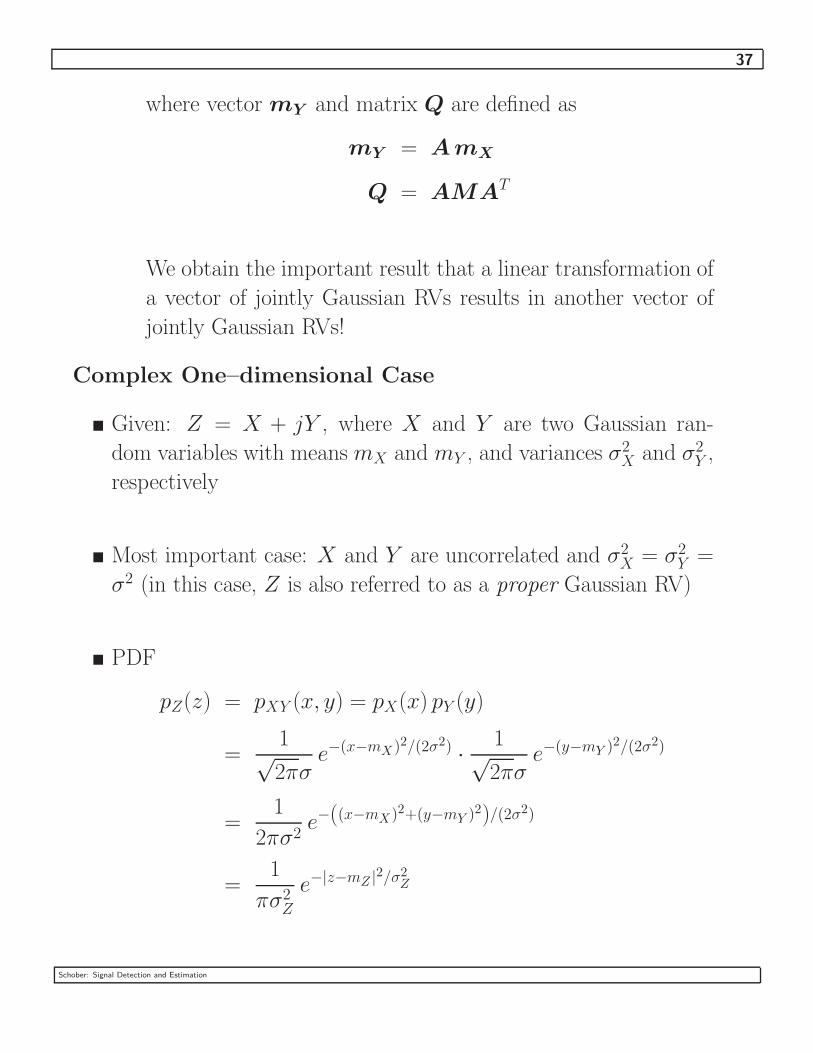
where vector mY and matrix Q are defined as

mY = A mX

Q = AMAT

We obtain the important result that a linear transformation of

a vector of jointly Gaussian RVs results in another vector of

jointly Gaussian RVs!

Complex One–dimensional Case

� Given: Z = X + jY , where X and Y are two Gaussian ran-

dom variables with means mX and mY , and variances σ2X and σ2

Y ,

respectively

� Most important case: X and Y are uncorrelated and σ2X = σ2

Y =

σ2 (in this case, Z is also referred to as a proper Gaussian RV)

� PDF

pZ(z) = pXY (x, y) = pX(x) pY (y)

=1√2πσ

e−(x−mX )2/(2σ2) · 1√2πσ

e−(y−mY )2/(2σ2)

=1

2πσ2e−((x−mX )2+(y−mY )2)/(2σ2)

=1

πσ2Z

e−|z−mZ |2/σ2Z


38

with

mZ = E{Z} = mX + jmY

and

σ2Z = E{|Z −mZ|2} = σ2

X + σ2Y = 2σ2

Complex Multi–dimensional Case

� Given: Complex vector Z = X + jY , where X and Y are two

real jointly Gaussian vectors with mean vectors mX and mY and

covariance matrices MX and MY , respectively

� Most important case: X and Y are uncorrelated and MX = MY

(proper complex random vector)

� PDF

pZ(z) =1

πn |MZ|exp

(

−(z − mZ)HM−1Z (z − mZ)

)

with

mZ = E{z} = mX + jmY

and

MZ = E{(z − mZ)(z − mZ)H} = MX + M Y


39

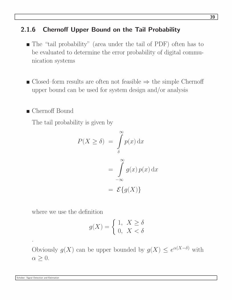
2.1.6 Chernoff Upper Bound on the Tail Probability

� The “tail probability” (area under the tail of PDF) often has to

be evaluated to determine the error probability of digital commu-

nication systems

� Closed–form results are often not feasible ⇒ the simple Chernoff

upper bound can be used for system design and/or analysis

� Chernoff Bound

The tail probability is given by

P (X ≥ δ) =

∞∫

δ

p(x) dx

=

∞∫

−∞

g(x) p(x) dx

= E{g(X)}

where we use the definition

g(X) =

{

1, X ≥ δ

0, X < δ

.

Obviously g(X) can be upper bounded by g(X) ≤ eα(X−δ) with

α ≥ 0.


40

1

eα(X−δ)

g(X)

Xδ

Therefore, we get the bound

P (X ≥ δ) = E{g(X)}

≤ E{eα(X−δ)}

= e−α δ E{eαX}

which is valid for any α ≥ 0. In practice, however, we are inter-

ested in the tightest upper bound. Therefore, we optimize α:

d

dαe−α δ E{eαX} = 0

The optimum α = αopt can be obtained from

E{X eαoptX} − δ E{eαoptX} = 0

The solution to this equation gives the Chernoff bound

P (X ≥ δ) ≤ e−αopt δ E{eαoptX}


41

2.1.7 Central Limit Theorem

� Given: n statistical independent and identically distributed RVs

Xi, i = 1, 2, . . . , n, with finite varuance. For simplicity, we as-

sume that the Xi have zero mean and identical variances σ2X . Note

that the Xi can have any PDF.

� We consider the sum

Y =1√n

n∑

i=1

Xi

� Central Limit Theorem

For n→ ∞ Y is a Gaussian RV with zero mean and variance σ2X .

Proof: See Textbook

� In practice, already for small n (e.g. n = 5) the distribution of Y

is very close to a Gaussian PDF.

� In practice, it is not necessary that all Xi have exactly the same

PDF and the same variance. Also the statistical independence of

different Xi is not necessary. If the PDFs and the variances of

the Xi are similar, for sufficiently large n the PDF of Y can be

approximated by a Gaussian PDF.

� The central limit theorem explains why many physical phenomena

follow a Gaussian distribution.


42

2.2 Stochastic Processes

� In communications many phenomena (noise from electronic de-

vises, transmitted symbol sequence, etc.) can be described as RVs

X(t) that depend on (continuous) time t. X(t) is referred to as a

stochastic process.

� A single realization of X(t) is a sample function. E.g. measure-

ment of noise voltage generated by a particular resistor.

� The collection of all sample functions is the ensemble of sample

functions. Usually, the size of the ensemble is infinite.

� If we consider the specific time instants t1 > t2 > . . . > tn with

the arbitrary positive integer index n, the random variables Xti =

X(ti), i = 1, 2, . . . , n, are fully characterized by their joint PDF

p(xt1, xt2, . . . , xtn).

� Stationary stochastic process:

Consider a second set Xti+τ = X(ti+ τ ), i = 1, 2, . . . , n, of RVs,

where τ is an arbitrary time shift. If Xti and Xti+τ have the same

statistical properties, X(t) is stationary in the strict sense. In

this case,

p(xt1, xt2, . . . , xtn) = p(xt1+τ , xt2+τ , . . . , xtn+τ)

is true, where p(xt1+τ , xt2+τ , . . . , xtn+τ ) denotes the joint PDF of

the RVs Xti+τ . If Xti and Xti+τ do not have the same statistical

properties, the process X(t) is nonstationary.


43

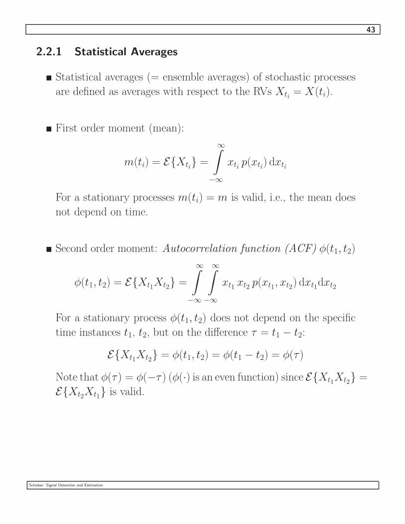
2.2.1 Statistical Averages

� Statistical averages (= ensemble averages) of stochastic processes

are defined as averages with respect to the RVs Xti = X(ti).

� First order moment (mean):

m(ti) = E{Xti} =

∞∫

−∞

xti p(xti) dxti

For a stationary processes m(ti) = m is valid, i.e., the mean does

not depend on time.

� Second order moment: Autocorrelation function (ACF) φ(t1, t2)

φ(t1, t2) = E{Xt1Xt2} =

∞∫

−∞

∞∫

−∞

xt1 xt2 p(xt1, xt2) dxt1dxt2

For a stationary process φ(t1, t2) does not depend on the specific

time instances t1, t2, but on the difference τ = t1 − t2:

E{Xt1Xt2} = φ(t1, t2) = φ(t1 − t2) = φ(τ )

Note that φ(τ ) = φ(−τ ) (φ(·) is an even function) since E{Xt1Xt2} =

E{Xt2Xt1} is valid.


44

Example:

ACF of an uncorrelated stationary process: φ(τ ) = δ(τ )

1

τ

φ(τ )

� Central second order moment: Covariance function µ(t1, t2)

µ(t1, t2) = E{(Xt1 −m(t1))(Xt2 −m(t2))}

= φ(t1, t2) −m(t1)m(t2)

For a stationary processes we get

µ(t1, t2) = µ(t1 − t2) = µ(τ ) = φ(τ ) −m2

� Stationary stochastic processes are asymptotically uncorrelated,

i.e.,

limτ→∞

µ(τ ) = 0


45

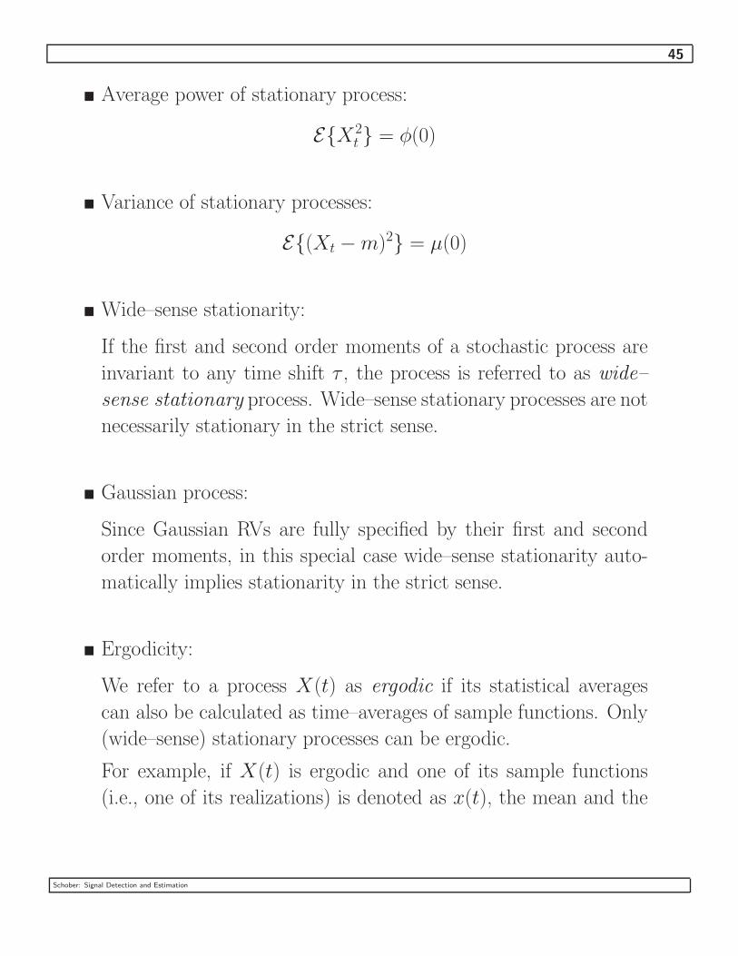
� Average power of stationary process:

E{X2t } = φ(0)

� Variance of stationary processes:

E{(Xt −m)2} = µ(0)

� Wide–sense stationarity:

If the first and second order moments of a stochastic process are

invariant to any time shift τ , the process is referred to as wide–

sense stationary process. Wide–sense stationary processes are not

necessarily stationary in the strict sense.

� Gaussian process:

Since Gaussian RVs are fully specified by their first and second

order moments, in this special case wide–sense stationarity auto-

matically implies stationarity in the strict sense.

� Ergodicity:

We refer to a process X(t) as ergodic if its statistical averages

can also be calculated as time–averages of sample functions. Only

(wide–sense) stationary processes can be ergodic.

For example, if X(t) is ergodic and one of its sample functions

(i.e., one of its realizations) is denoted as x(t), the mean and the


46

ACF can be calulated as

m = limT→∞

1

2T

T∫

−T

x(t) dt

and

φ(τ ) = limT→∞

1

2T

T∫

−T

x(t)x(t+ τ ) dt,

respectively. In practice, it is usually assumed that a process is

(wide–sense) stationary and ergodic. Ergodicity is important since

in practice only sample functions of a stochastic process can be

observed!

Averages for Jointly Stochastic Processes

� Let X(t) and Y (t) denote two stochastic processes and consider

the RVs Xti = X(ti), i = 1, 2, . . . , n, and Yt′j

= Y (t′j), j =

1, 2, . . . , m at times t1 > t2 > . . . > tn and t′1 > t′2 > . . . > t′m,

respectively. The two stochastic processes are fully characterized

by their joint PDF

p(xt1, xt2, . . . , xtn, yt′1, yt′2, . . . , yt′m)

� Joint stationarity: X(t) and Y (t) are jointly stationary if their

joint PDF is invariant to time shifts τ for all n and m.


47

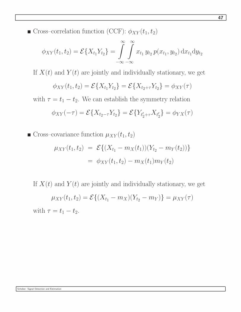
� Cross–correlation function (CCF): φXY (t1, t2)

φXY (t1, t2) = E{Xt1Yt2} =

∞∫

−∞

∞∫

−∞

xt1 yt2 p(xt1, yt2) dxt1dyt2

If X(t) and Y (t) are jointly and individually stationary, we get

φXY (t1, t2) = E{Xt1Yt2} = E{Xt2+τYt2} = φXY (τ )

with τ = t1 − t2. We can establish the symmetry relation

φXY (−τ ) = E{Xt2−τYt2} = E{Yt′2+τXt′2} = φY X(τ )

� Cross–covariance function µXY (t1, t2)

µXY (t1, t2) = E{(Xt1 −mX(t1))(Yt2 −mY (t2))}

= φXY (t1, t2) −mX(t1)mY (t2)

If X(t) and Y (t) are jointly and individually stationary, we get

µXY (t1, t2) = E{(Xt1 −mX)(Yt2 −mY )} = µXY (τ )

with τ = t1 − t2.


48

� Statistical independence

Two processes X(t) and Y (t) are statistical independent if and

only if

p(xt1, xt2, . . . , xtn, yt′1, yt′2, . . . , yt′m) =

p(xt1, xt2, . . . , xtn) p(yt′1, yt′2, . . . , yt′m)

is valid for all n and m.

� Uncorrelated processes

Two processes X(t) and Y (t) are uncorrelated if and only if

µXY (t1, t2) = 0

holds.

Complex Stochastic Processes

� Given: Complex random process Z(t) = X(t) + jY (t) with real

random processes X(t) and Y (t)

� Similarly to RVs, we treat Z(t) as a tupel of X(t) and Y (t), i.e.,

the PDF of Zti = Z(ti), 1, 2, . . . , n is given by

pZ(zt1, zt2, . . . , ztn) = pXY (xt1, xt2, . . . , xtn, yt1, yt2, . . . , ytn)

� We define the ACF of a complex–valued stochastic process Z(t)


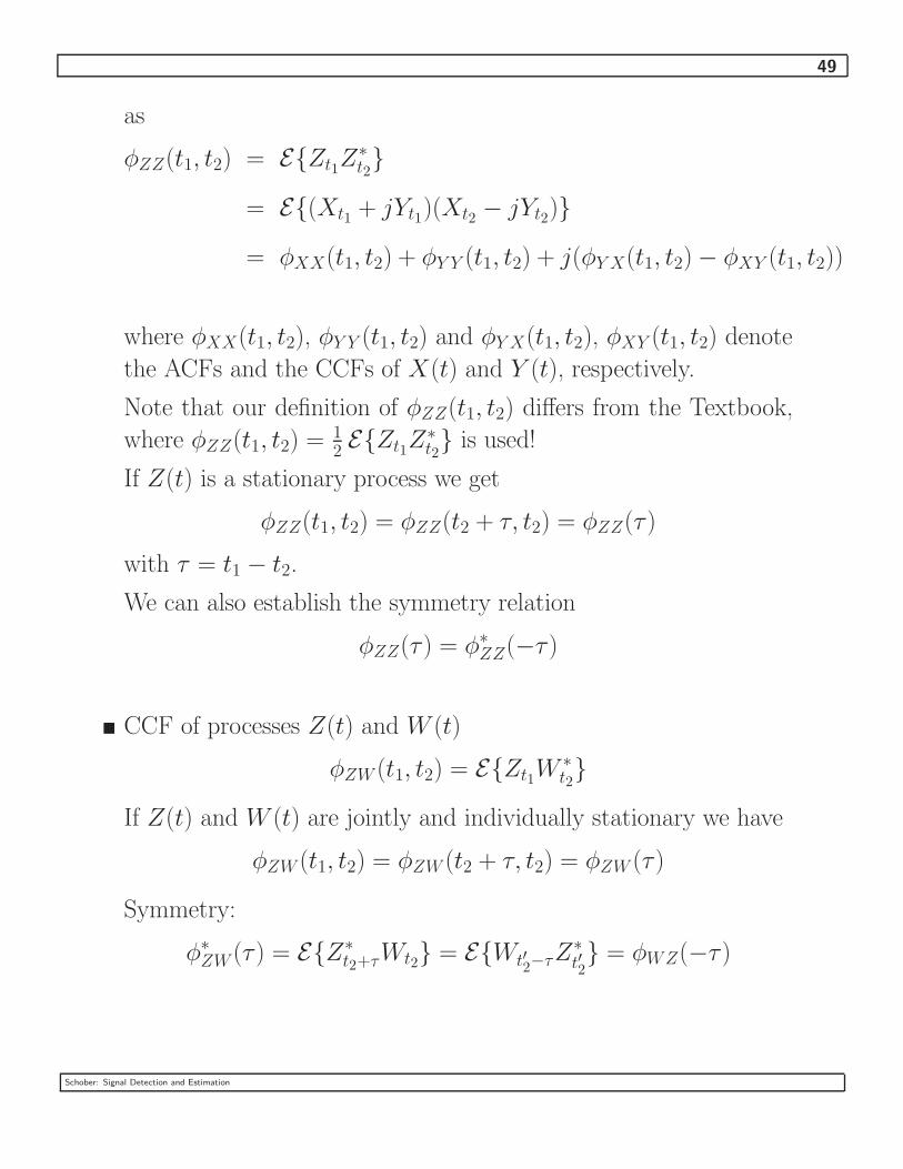
49

as

φZZ(t1, t2) = E{Zt1Z∗t2}

= E{(Xt1 + jYt1)(Xt2 − jYt2)}

= φXX(t1, t2) + φY Y (t1, t2) + j(φY X(t1, t2) − φXY (t1, t2))

where φXX(t1, t2), φY Y (t1, t2) and φY X(t1, t2), φXY (t1, t2) denote

the ACFs and the CCFs of X(t) and Y (t), respectively.

Note that our definition of φZZ(t1, t2) differs from the Textbook,

where φZZ(t1, t2) = 12E{Zt1Z∗

t2} is used!

If Z(t) is a stationary process we get

φZZ(t1, t2) = φZZ(t2 + τ, t2) = φZZ(τ )


We can also establish the symmetry relation

φZZ(τ ) = φ∗ZZ(−τ )

� CCF of processes Z(t) and W (t)

φZW (t1, t2) = E{Zt1W ∗t2}

If Z(t) and W (t) are jointly and individually stationary we have

φZW (t1, t2) = φZW (t2 + τ, t2) = φZW (τ )

Symmetry:

φ∗ZW (τ ) = E{Z∗t2+τ

Wt2} = E{Wt′2−τZ∗t′2} = φWZ(−τ )


50

2.2.2 Power Density Spectrum

� The Fourier spectrum of a random process does not exist.

� Instead we define the power spectrum of a stationary stochastic

process as the Fourier transform F{·} of the ACF

Φ(f) = F{φ(τ )} =

∞∫

−∞

φ(τ ) e−j2πfτ dτ

Consequently, the ACF can be obtained from the power spectrum

(also referred to as power spectral density) via inverse Fourier

transform F−1{·} as

φ(τ ) = F−1{Φ(f)} =

∞∫

−∞

Φ(f) ej2πfτ df

Example:

Power spectrum of an uncorrelated stationary process:

Φ(f) = F{δ(τ )} = 1

1

f

Φ(f)


51

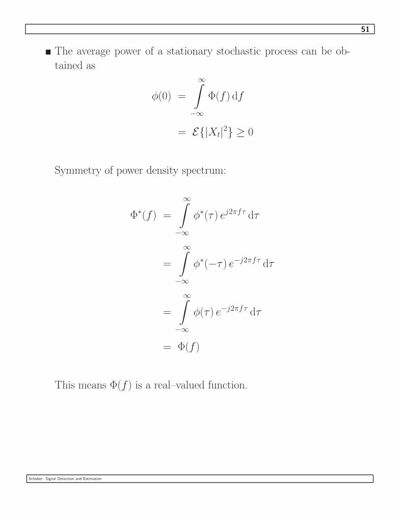
� The average power of a stationary stochastic process can be ob-

tained as

φ(0) =

∞∫

−∞

Φ(f) df

= E{|Xt|2} ≥ 0

Symmetry of power density spectrum:

Φ∗(f) =

∞∫

−∞

φ∗(τ ) ej2πfτ dτ

=

∞∫

−∞

φ∗(−τ ) e−j2πfτ dτ

=

∞∫

−∞

φ(τ ) e−j2πfτ dτ

= Φ(f)

This means Φ(f) is a real–valued function.


52

� Cross–correlation spectrum

Consider the random processes X(t) and Y (t) with CCF φXY (τ ).

The cross–correlation spectrum ΦXY (f) is defined as

ΦXY (f) =

∞∫

−∞

φXY (τ ) e−j2πfτ dτ

It can be shown that the symmetry relation Φ∗XY (f) = ΦY X(f)

is valid. If X(t) and Y (t) are real stochastic processes ΦY X(f) =

ΦXY (−f) holds.

2.2.3 Response of a Linear Time–Invariant System to a Ran-

dom Input Signal

� We consider a deterministic linear time–invariant system fully de-

scribed by its impulse response h(t), or equivalently by its fre-

quency response

H(f) = F{h(t)} =

∞∫

−∞

h(t) e−j2πft dt

� Let the signal x(t) be the input to the system h(t). Then the

output y(t) of the system can be expressed as

y(t) =

∞∫

−∞

h(τ ) x(t− τ ) dτ


53

In our case x(t) is a sample function of a (stationary) stochastic

processX(t) and therefore, y(t) is a sample function of a stochastic

process Y (t). We are interested in the mean and the ACF of Y (t).

� Mean of Y (t)

mY = E{Y (t)} =

∞∫

−∞

h(τ ) E{X(t− τ )} dτ

= mX

∞∫

−∞

h(τ ) dτ = mX H(0)

� ACF of Y (t)

φY Y (t1, t2) = E{Yt1Y ∗t2}

=

∞∫

−∞

∞∫

−∞

h(α)h∗(β) E{X(t1 − α)X∗(t2 − β)} dα dβ

=

∞∫

−∞

∞∫

−∞

h(α)h∗(β)φXX(t1 − t2 + β − α) dα dβ

=

∞∫

−∞

∞∫

−∞

h(α)h∗(β)φXX(τ + β − α) dα dβ

= φY Y (τ )


54

Here, we have used τ = t1 − t2 and the last line indicates that if

the input to a linear time–invariant system is stationary, also the

output will be stationary.

If we define the deterministic system ACF as

φhh(τ ) = h(τ ) ∗ h∗(−τ ) =

∞∫

−∞

h∗(t)h(t + τ ) dt,

where ”∗” is the convolution operator, then we can rewrite φY Y (τ )

elegantly as

φY Y (τ ) = φhh(τ ) ∗ φXX(τ )

� Power spectral density of Y (t)

Since the Fourier transform of φhh(τ ) = h(τ ) ∗ h∗(−τ ) is

Φhh(f) = F{φhh(τ )} = F{h(τ ) ∗ h∗(−τ )}

= F{h(τ )}F{h∗(−τ )}

= |H(f)|2,

it is easy to see that the power spectral density of Y (t) is

ΦY Y (f) = |H(f)|2 ΦXX(f)

Since φY Y (0) = E{|Yt|2} = F−1{ΦY Y (f)}|τ=0,

φY Y (0) =

∞∫

−∞

ΦXX(f)|H(f)|2 df ≥ 0


55

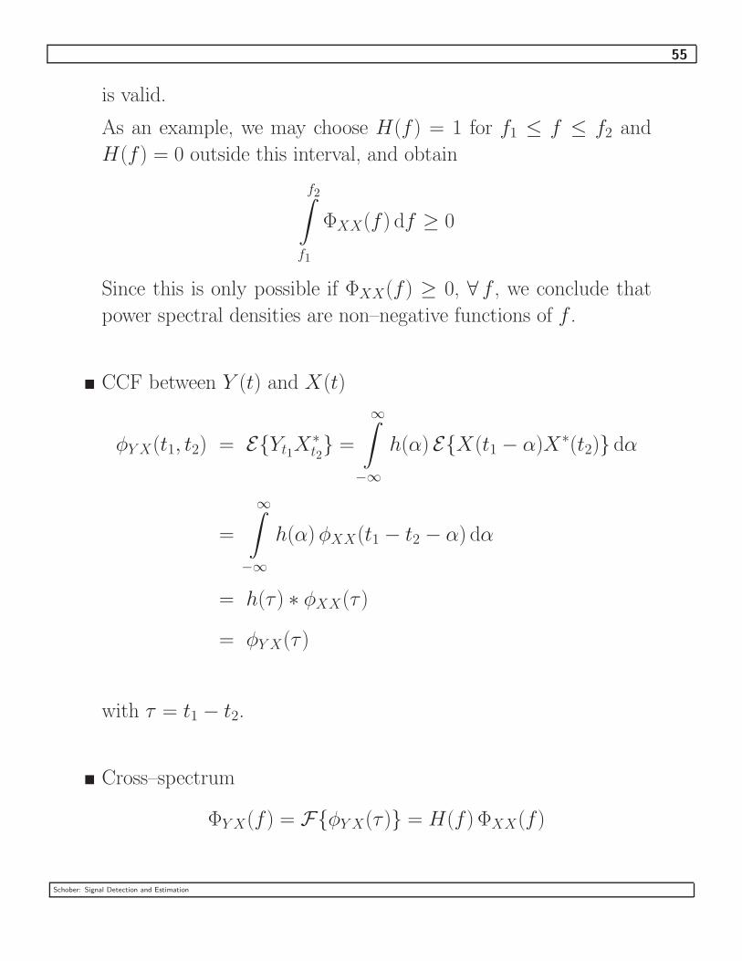
is valid.

As an example, we may choose H(f) = 1 for f1 ≤ f ≤ f2 and

H(f) = 0 outside this interval, and obtain

f2∫

f1

ΦXX(f) df ≥ 0

Since this is only possible if ΦXX(f) ≥ 0, ∀ f , we conclude that

power spectral densities are non–negative functions of f .

� CCF between Y (t) and X(t)

φY X(t1, t2) = E{Yt1X∗t2} =

∞∫

−∞

h(α) E{X(t1 − α)X∗(t2)} dα

=

∞∫

−∞

h(α)φXX(t1 − t2 − α) dα

= h(τ ) ∗ φXX(τ )

= φY X(τ )


� Cross–spectrum

ΦY X(f) = F{φY X(τ )} = H(f) ΦXX(f)


56

2.2.4 Sampling Theorem for Band–Limited Stochastic Pro-

cesses

� A deterministic signal s(t) is called band–limited if its Fourier

transform S(f) = F{s(t)} vanishes identically for |f | > W . If

we sample s(t) at a rate higher than fs ≥ 2W , we can reconstruct

s(t) from the samples s(n/(2W )), n = 0, ±1, ±2, . . ., using an

ideal low–pass filter with bandwidth W .

� A stationary stochastic process X(t) is band–limited if its power

spectrum Φ(f) vanishes identically for |f | > W , i.e., Φ(f) = 0 for

|f | > W . Since Φ(f) is the Fourier transform of φ(τ ), φ(τ ) can be

reconstructed from the samples φ(n/(2W )), n = 0, ±1, ±2, . . .:

φ(τ ) =

∞∑

n=−∞φ

( n

2W

)

sin [2πW (τ − n/(2W ))]

2πW (τ − n/(2W ))

h(t) = sin(2πWt)/(2πWt) is the impulse response of an ideal

low–pass filter with bandwidth W .

If X(t) is a band–limited stationary stochastic process, then we

can represent X(t) as

X(t) =∞

∑

n=−∞X

( n

2W

)

sin [2πW (t− n/(2W ))]

2πW (t− n/(2W )),

whereX(n/(2W )) are the samples ofX(t) at times n = 0, ±1, ±2, . . .


57

2.2.5 Discrete–Time Stochastic Signals and Systems

� Now, we consider discrete–time (complex) stochastic processesX [n]

with discrete–time n which is an integer. Sample functions of X [n]

are denoted by x[n]. X [n] may be obtained from a continuous–

time process X(t) by sampling X [n] = X(nT ), T > 0.

� X [n] can be characterized in a similar way as the continuous–time

process X(t).

� ACF

φ[n, k] = E{XnX∗k} =

∞∫

−∞

∞∫

−∞

xnx∗k p(xn, xk) dxndxk

If X [n] is stationary, we get

φ[λ] = φ[n, k] = φ[n, n− λ]

The average power of the stationary process X [n] is defined as

E{|Xn|2} = φ[0]

� Covariance function

µ[n, k] = φ[n, k] − E{Xn}E{X∗k}

If X [n] is stationary, we get

µ[λ] = φ[λ] − |mX |2,where mX = E{Xn} denotes the mean of X [n].


58

� Power spectrum

The power spectrum of X [n] is the (discrete–time) Fourier trans-

form of the ACF φ[λ]

Φ(f) = F{φ[λ]} =∞

∑

λ=−∞φ[λ]e−j2πfλ

and the inverse transform is

φ[λ] = F−1{Φ(f)} =

1/2∫

−1/2

Φ(f) ej2πfλ df

Note that Φ(f) is periodic with a period fd = 1, i.e., Φ(f + k) =

Φ(f) for k = ±1, ±2, . . .

Example:

Consider a stochastic process with ACF

φ[λ] = p δ[λ + 1] + δ[λ] + p δ[λ− 1]

with constant p. The corresponding power spectrum is given

by

Φ(f) = F{φ[λ]} = 1 + 2cos(2πf).

Note that φ[λ] is a valid ACF if and only if −1/2 ≤ p ≤ 1/2.


59

� Response of a discrete–time linear time–invariant system

– Discrete–time linear time–invariant system is described by its

impulse response h[n]

– Frequency response

H(f) = F{h[n]} =∞

∑

n=−∞h[n] e−j2πfn

– Response y[n] of system to sample function x[n]

y[n] = h[n] ∗ x[n] =

∞∑

k=−∞h[k]x[n− k]

where ∗ denotes now discrete–time convolution.

– Mean of Y [n]

mY = E{Y [n]} =

∞∑

k=−∞h[k] E{X [n− k]}

= mX

∞∑

k=−∞h[k]

= mX H(0)

where mX is the mean of X [n].


60

– ACF of Y [n]

Using the deterministic ”system” ACF

φhh[λ] = h[λ] ∗ h∗[−λ] =

∞∑

k=−∞h∗[k]h[k + λ]

it can be shown that φY Y [λ] can be expressed as

φY Y [λ] = φhh[λ] ∗ φXX [λ]

– Power spectrum of Y [n]

ΦY Y (f) = |H(f)|2 ΦXX(f)

2.2.6 Cyclostationary Stochastic Processes

� An important class of nonstationary processes are cyclostationary

processes. Cyclostationary means that the statistical averages of

the process are periodic.

� Many digital communication signals can be expressed as

X(t) =∞

∑

n=−∞a[n] g(t− nT )

where a[n] denotes the transmitted symbol sequence and can be

modeled as a (discrete–time) stochastic process with ACF φaa[λ] =

E{a∗[n]a[n+λ]}. g(t) is a deterministic function. T is the symbol

duration.


61

� Mean of X(t)

mX(t) = E{X(t)}

=

∞∑

n=−∞E{a[n]} g(t− nT )

= ma

∞∑

n=−∞g(t− nT )

where ma is the mean of a[n]. Observe that mX(t+kT ) = mX(t),

i.e., mX(t) has period T .

� ACF of X(t)

φXX(t + τ, t) = E{X(t+ τ )X∗(t)}

=∞

∑

n=−∞

∞∑

m=−∞E{a∗[n]a[m]} g∗(t− nT )g(t + τ −mT )

=∞

∑

n=−∞

∞∑

m=−∞φaa[m− n] g∗(t− nT )g(t + τ −mT )

Observe again that

φXX(t + τ + kT, t + kT ) = φXX(t + τ, t)

and therefore the ACF has also period T .


62

� Time–average ACF

The ACF φXX(t+τ, t) depends on two parameters t and τ . Often

we are only interested in the time–average ACF defined as

φXX(τ ) =1

T

T/2∫

−T/2

φXX(t + τ, t) dt

� Average power spectrum

ΦXX(f) = F{φXX(τ )} =

∞∫

−∞

φXX(τ ) e−j2πfτ dτ


2 Probability and Stochastic Processes - University of …courses.ece.ubc.ca/564/chapter2.pdf9 2...

Documents

Transcript of 2 Probability and Stochastic Processes - University of …courses.ece.ubc.ca/564/chapter2.pdf9 2...